3D Common Corruptions and Data Augmentation

Abstract

We introduce a set of image transformations that can be used as corruptions to evaluate the robustness of models as well as data augmentation mechanisms for training neural networks. The primary distinction of the proposed transformations is that, unlike existing approaches such as Common Corruptions [27], the geometry of the scene is incorporated in the transformations – thus leading to corruptions that are more likely to occur in the real world. We also introduce a set of semantic corruptions (e.g. natural object occlusions. See Fig. 1).

We show these transformations are ‘efficient’ (can be computed on-the-fly), ‘extendable’ (can be applied on most image datasets), expose vulnerability of existing models, and can effectively make models more robust when employed as ‘3D data augmentation’ mechanisms. The evaluations on several tasks and datasets suggest incorporating 3D information into benchmarking and training opens up a promising direction for robustness research.

1 Introduction

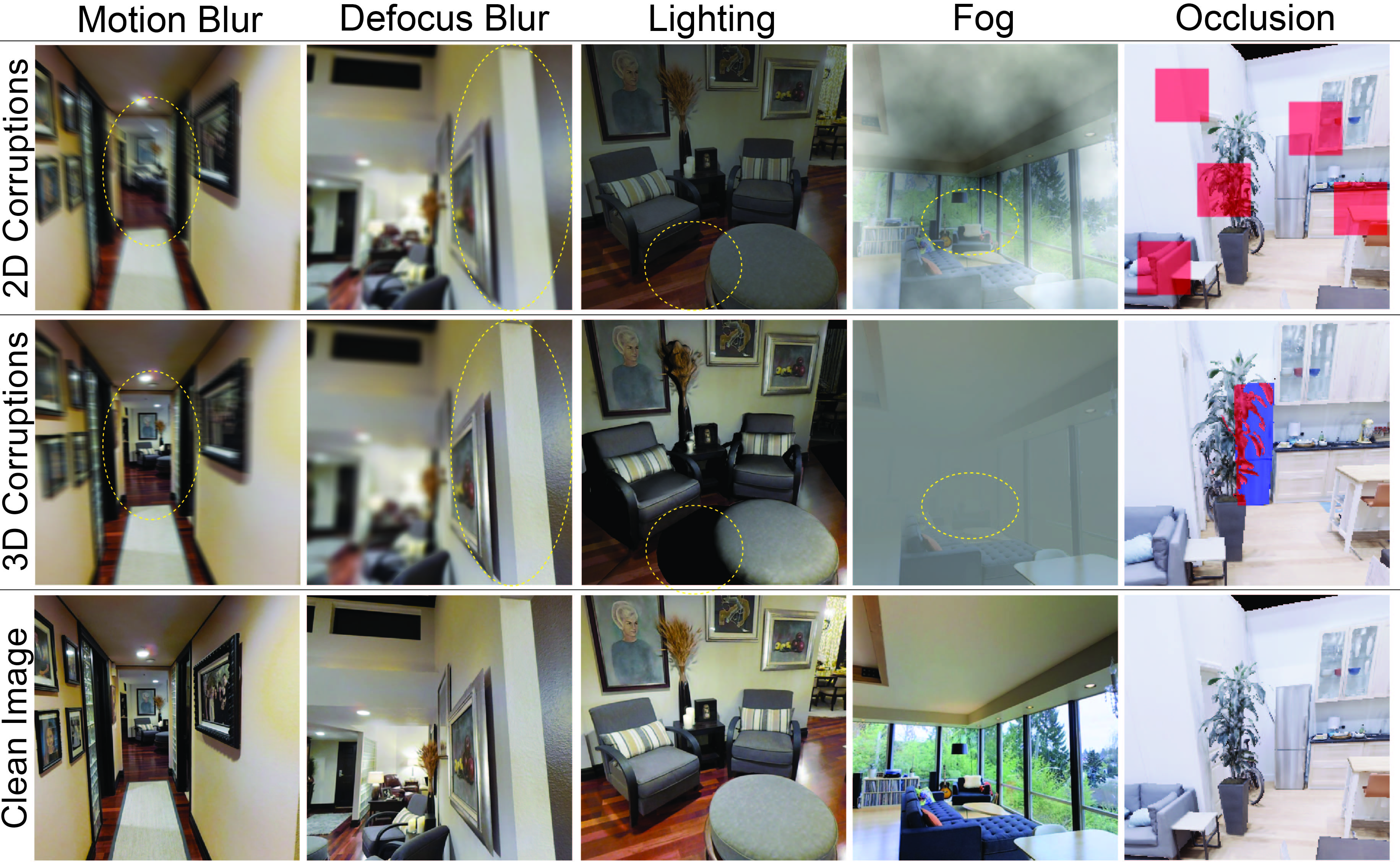
Figure 1: Using 3D information to generate real-world corruptions. The top row shows sample 2D corruptions applied uniformly over the image, e.g. as in Common Corruptions [27], disregarding 3D information. This leads to corruptions that are unlikely to happen in the real world, e.g. having the same motion blur over the entire image irrespective of the distance to camera (top left). Middle row shows their 3D counterparts from 3D Common Corruptions (3DCC). The circled regions highlight the effect of incorporating 3D information. More specifically, in 3DCC, 1. motion blur has a motion parallax effect where objects further away from the camera seem to move less, 2. defocus blur has a depth of field effect, akin to a large aperture effect in real cameras, where certain regions of the image can be selected to be in focus, 3. lighting takes the scene geometry into account when illuminating the scene and casts shadows on objects, 4. fog gets denser further away from the camera, 5. occlusions of a target object, e.g. fridge (blue mask), are created by changing the camera’s viewpoint and having its view naturally obscured by another object, e.g. the plant (red mask). This is in contrast to its 2D counterpart that randomly discards patches [13]. See project page for a video version of the figure.

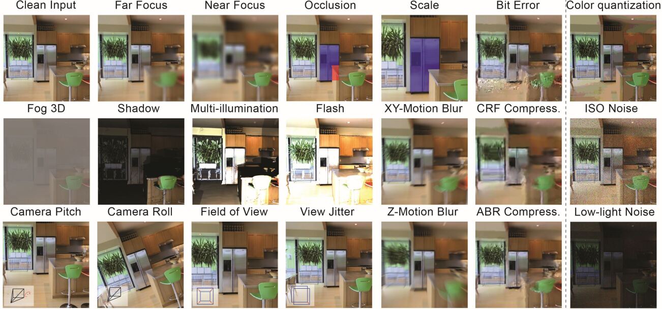
Figure 2: The new corruptions. We propose a diverse set of new corruption operations ranging from defocusing (near/far focus) to lighting changes and 3D-semantic ones, e.g. object occlusion. These corruptions are all automatically generated, efficient to compute, and can be applied to most datasets (Sec. 3.3). We show that they expose vulnerabilities in models (Sec. 5.2.1) and are a good approximation of realistic corruptions (Sec. 5.2.3). A subset of the corruptions marked in the last column are novel and commonly faced in the real world, but are not 3D based. We include them in our benchmark. For occlusion and scale corruptions, the blue and red masks denote the amodal visible and occluded parts of an object, e.g. the fridge.

Computer vision models deployed in the real world will encounter naturally occurring distribution shifts from their training data. These shifts range from lower-level distortions, such as motion blur and illumination changes, to semantic ones, like object occlusion. Each of them represents a possible failure mode of a model and has been frequently shown to result in profoundly unreliable predictions [15, 27, 67, 31, 23]. Thus, a systematic testing of vulnerabilities to these shifts is critical before deploying these models in the real world.

This work presents a set of distribution shifts in order to test models’ robustness. In contrast to previously proposed shifts which perform uniform 2D modifications over the image, such as Common Corruptions (2DCC) [27], our shifts incorporate 3D information to generate corruptions that are consistent with the scene geometry. This leads to shifts that are more likely to occur in the real world (See Fig. 1). The resulting set includes 20 corruptions, each representing a distribution shift from training data, which we denote as 3D Common Corruptions (3DCC). 3DCC addresses several aspects of the real world, such as camera motion, weather, occlusions, depth of field, and lighting. Figure 2 provides an overview of all corruptions. As shown in Fig. 1, the corruptions in 3DCC are more diverse and realistic compared to 2D-only approaches.

We show in Sec. 5 that the performance of the methods aiming to improve robustness, including those with diverse data augmentation, reduce drastically under 3DCC. Furthermore, we observe that the robustness issues exposed by 3DCC well correlate with corruptions generated via photorealistic synthesis. Thus, 3DCC can serve as a challenging testbed for real-world corruptions, especially those that depend on scene geometry.

Motivated by this, our framework also introduces new 3D data augmentations. They take the scene geometry into account, as opposed to 2D augmentations, thus enabling models to build invariances against more realistic corruptions. We show in Sec. 5.3 that they significantly boost model robustness against such corruptions, including the ones that cannot be addressed by the 2D augmentations.

The proposed corruptions are generated programmatically with exposed parameters, enabling fine-grained analysis of robustness, e.g. by continuously increasing the 3D motion blur. They are efficient to compute and can be computed on-the-fly during training as data augmentation with a small increase in computational cost. They are also extendable, i.e. they can be applied to standard vision datasets, e.g. ImageNet [12], that do not come with 3D labels.

2 Related Work

This work presents a data-focused approach [63, 52] to robustness. We give an overview of some of the related topics within the constraints of space.

Robustness benchmarks based on corruptions: Several studies have proposed robustness benchmarks to understand the vulnerability of models to corruptions. A popular benchmark, Common Corruptions (2DCC) [27], generates synthetic corruptions on real images that expose sensitivities of image recognition models. It led to a series of works either creating new corruptions or applying similar corruptions on other datasets for different tasks [32, 43, 7, 80, 45, 66]. In contrast to these works, 3DCC modifies real images using 3D information to generate realistic corruptions. The resulting images are both perceptually different and expose different failure modes in model predictions compared to their 2D counterparts (See Fig. 1 and 8). Other works create and capture the corruptions in the real world, e.g. ObjectNet [3]. Although being realistic, it requires significant manual effort and is not extendable. A more scalable approach is to use computer graphics based 3D simulators to generate corrupted data [38] which can lead to generalization concerns. 3DCC aims to generate corruptions as close to the real world as possible while staying scalable.

Robustness analysis works use existing benchmarks to probe the robustness of different methods, e.g. data augmentation or self-supervised training, under several distribution shifts. Recent works investigated the relation between synthetic and natural distribution shifts [68, 26, 44, 14] and effectiveness of architectural advancements [5, 64, 48]. We select several popular methods to show that 3DCC can serve as a challenging benchmark (Fig. 6 and  7).

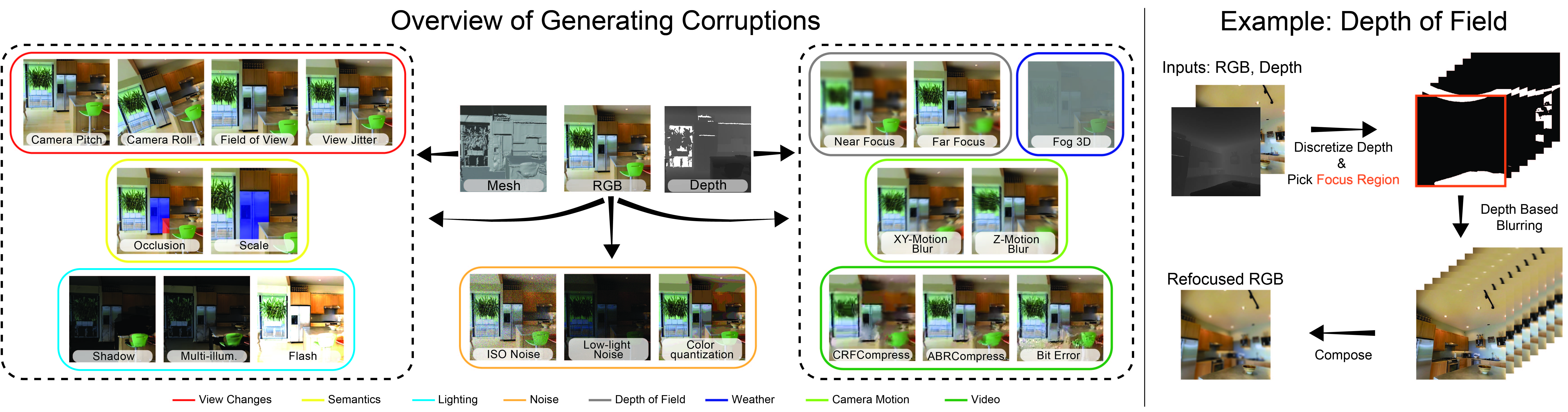
Figure 3: Left: We show the inputs needed to create each of our corruptions, e.g. the 3D information such as depth, and RGB image. These corruptions have also been grouped (in solid colored lines) according to their corruption types. For example, to create the distortions in the dashed box in the right, one only needs the RGB image and its corresponding depth. For the ones in the left dashed box, 3D mesh is required. Note that one can create view changes corruptions also from panoramic images if available, without a mesh. Right: As an example, we show an overview of generating depth of field effect efficiently. The scene is first split into multiple layers by discretizing scene depth. Next, a region is chosen to be kept in focus (here it is the region closest to the camera). We then compute the corresponding blur levels for each layer according to their distance from the focus region, using a pinhole camera model. The final refocused image is obtained by compositing blurred image layers.

Improving robustness: Numerous methods have been proposed to improve model robustness such as data augmentation with corrupted data [22, 41, 40, 60], texture changes [24, 26], image compositions [85, 82] and transformations [29, 81]. While these methods can generalize to some unseen examples, performance gains are non-uniform [61, 22]. Other methods include self-training [76], pre-training [28, 50], architectural changes [5, 64], and diverse ensembling [51, 33, 78, 79]. Here we instead adopt a data-focused approach to robustness by i. providing a large set of realistic distribution shifts and ii. introducing new 3D data augmentation that improves robustness against real-world corruptions (Sec. 5.3).

Photorealistic image synthesis involves techniques to generate realistic images. Some of these techniques have been recently used to create corruption data. These techniques are generally specific to a single real-world corruption. Examples include adverse weather conditions [19, 62, 70, 30, 69], motion blur [6, 49], depth of field [53, 72, 71, 17, 4], lighting [77, 25], and noise [21, 74]. They may be used for purely artistic purposes or to create training data. Some of our 3D transformations are instantiations of these methods, with the downstream goal of testing and improving model robustness in a unified framework with a wide set of corruptions.

Image restoration aims to undo the corruption in the image using classical signal processing techniques [35, 20, 18, 42] or learning-based approaches [86, 8, 46, 87, 57, 47, 1]. We differ from these works by generating corrupted data, rather than removing it, to use them for benchmarking or data augmentation. Thus, in the latter, we train with these corrupted data to encourage the model to be invariant to corruptions, as opposed to training the model to remove the corruptions as a pre-processing step.

Adversarial corruptions add imperceptible worst-case shifts to the input to fool a model [67, 36, 41, 11]. Most of the failure cases of models in the real world are not the result of adversarial corruptions but rather naturally occurring distribution shifts. Thus, our focus in this paper is to generate corruptions that are likely to occur in the real world.

3 Generating 3D Common Corruptions

3.1 Corruption Types

We define different corruption types, namely depth of field, camera motion, lighting, video, weather, view changes, semantics, and noise, resulting in 20 corruptions in 3DCC. Most of the corruptions require an RGB image and scene depth, while some needs 3D mesh (See Fig. 3). We use a set of methods leveraging 3D synthesis techniques or image formation models to generate different corruption types, as explained in more detail below. Further details are provided in the supplementary.

Depth of field corruptions create refocused images. They keep a part of the image in focus while blurring the rest. We consider a layered approach [17, 4] that splits the scene into multiple layers. For each layer, the corresponding blur level is computed using the pinhole camera model. The blurred layers are then composited with alpha blending. Figure 3 (right) shows an overview of the process. We generate near focus and far focus corruptions by randomly changing the focus region to the near or far part of the scene.

Camera motion creates blurry images due to camera movement during exposure. To generate this effect, we first transform the input image into a point cloud using the depth information. Then, we define a trajectory (camera motion) and render novel views along this trajectory. As the point cloud was generated from a single RGB image, it has incomplete information about the scene when the camera moves. Thus, the rendered views will have disocclusion artifacts. To alleviate this, we apply an inpainting method from [49]. The generated views are then combined to obtain parallax-consistent motion blur. We define XY-motion blur and Z-motion blur when the main camera motion is along the image XY-plane or Z-axis, respectively.

Lighting corruptions change scene illumination by adding new light sources and modifying the original illumination. We use Blender [10] to place these new light sources and compute the corresponding illumination for a given viewpoint in the 3D mesh. For the flash corruption, a light source is placed at the camera’s location, while for shadow corruption, it is placed at random diverse locations outside the camera frustum. Likewise, for multi-illumination corruption, we compute the illumination from a set of random light sources with different locations and luminosities.

Video corruptions arise during the processing and streaming of videos. Using the scene 3D, we create a video using multiple frames from a single image by defining a trajectory, similar to motion blur. Inspired by [80], we generate average bit rate (ABR) and constant rate factor (CRF) as H.265 codec compression artifacts, and bit error to capture corruptions induced by imperfect video transmission channel. After applying the corruptions over the video, we pick a single frame as the final corrupted image.

Weather corruptions degrade visibility by obscuring parts of the scene due to disturbances in the medium. We define a single corruption and denote it as fog 3D to differentiate it from the fog corruption in 2DCC. We use the standard optical model for fog [19, 62, 70]:

$$\mathbf{I(x)}~{}=~{}\mathbf{R(x)}\mathbf{t}(\mathbf{x})+\mathbf{A}(1-\mathbf{t}(\mathbf{x})),$$ (1)

where $\mathbf{I(x)}$ is the resulting foggy image at pixel $x$, $\mathbf{R(x)}$ is the clean image, $\mathbf{A}$ is atmospheric light, and $\mathbf{t}(\mathbf{x})$ is the transmission function describing the amount of light that reaches the camera. When the medium is homogeneous, the transmission depends on the distance from the camera, $\mathbf{t}(\mathbf{x})=\exp{(-\beta\mathbf{d}(\mathbf{x}))}$ where $\mathbf{d}(\mathbf{x})$ is the scene depth and $\beta$ is the attenuation coefficient controlling the fog thickness.

View changes are due to variations in the camera extrinsics and focal length. Our framework enables rendering RGB images conditioned on several changes, such as field of view, camera roll and camera pitch, using Blender. This enables us to analyze the sensitivity of models to various view changes in a controlled manner. We also generate images with view jitter that can be used to analyze if models predictions flicker with slight changes in viewpoint.

Semantics: In addition to view changes, we also render images by selecting an object in the scene and changing its occlusion level and scale. In occlusion corruption, we generate views of an object occluded by other objects. This is in contrast to random 2D masking of pixels to create an unnatural occlusion effect that is irrespective of image content, e.g. as in [13, 48] (See Fig. 1). Occlusion rate can be controlled to probe model robustness against occlusion changes. Similarly, in scale corruption, we render views of an object with varying distances from the camera location. Note that the corruptions require a mesh with semantic annotations, and are generated automatically, similar to [2]. This is in contrast to [3] which requires tedious manual effort. The objects can be selected by randomly picking a point in the scene or using the semantic annotations.

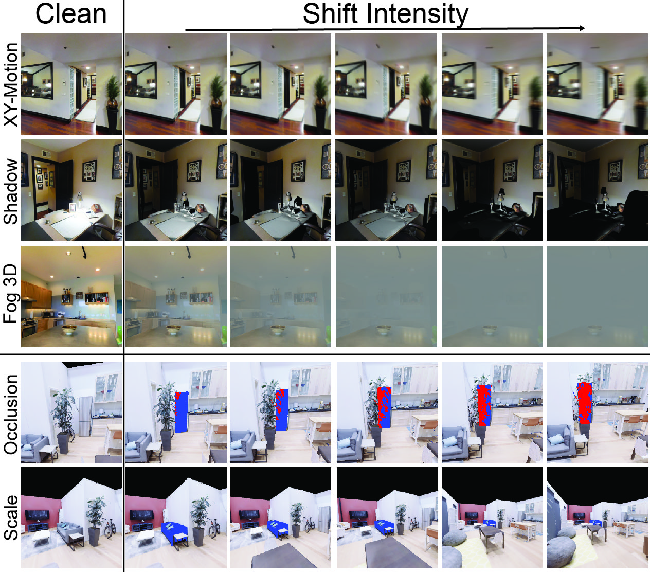
Figure 4: Visualizations of 3DCC with increasing shift intensities. Top: Increasing the shift intensity results in larger blur, less illumination, and denser fog. Bottom: The object becomes more occluded or shrinks in size using calculated viewpoint changes. The blue mask denotes the amodal visible parts of the fridge/couch, and the red mask is the occluded part. The leftmost column shows the clean images. Visuals for all corruptions for all shift intensities are shown in the supplementary.

Noise corruptions arise from imperfect camera sensors. We introduce new noise corruptions that do not exist in the previous 2DCC benchmark. For low-light noise, we decreased the pixel intensities and added Poisson-Gaussian distributed noise to reflect the low-light imaging setting [21]. ISO noise also follows a Poisson-Gaussian distribution, with a fixed photon noise (modeled by a Poisson), and varying electronic noise (modeled by a Gaussian). We also included color quantization as another corruption that reduces the bit depth of the RGB image. Only this subset of our corruptions is not based on 3D information.

3.2 Starter 3D Common Corruptions Dataset

We release the full open source code of our pipeline, which enables using the implemented corruptions on any dataset. As a starter dataset, we applied the corruptions on 16k Taskonomy [84] test images. For all the corruptions except the ones in view changes and semantics which change the scene, we follow the protocol in 2DCC and define 5 shift intensities, resulting in approximately 1 million corrupted images ($16$k$\times 14\times 5$). Directly applying the methods to generate corruptions results in uncalibrated shift intensities with respect to 2DCC. Thus, to enable aligned comparison with 2DCC on a more uniform intensity change, we perform a calibration step. For the corruptions with a direct counterpart in 2DCC, e.g. motion blur, we set the corruption level in 3DCC such that for each shift intensity in 2DCC, the average SSIM [73] values over all images is the same in both benchmarks. For the corruptions that do not have a counterpart in 2DCC, we adjust the distortion parameters to increase shift intensity while staying in a similar SSIM range as the others. For view changes and semantics, we render 32k images with smoothly changing parameters, e.g. roll angle, using the Replica [65] dataset. Figure 4 shows example corruptions with different shift intensities.

3.3 Applying 3DCC to standard vision datasets

While we employed datasets with full scene geometry information such as Taskonomy [84], 3DCC can also be applied to standard datasets without 3D information. We exemplify this on ImageNet [12] and COCO [39] validation sets by leveraging depth predictions from the MiDaS [55] model, a state-of-the-art depth estimator. Figure 5 shows example images with near focus, far focus, and fog 3D corruptions. Generated images are physically plausible, demonstrating that 3DCC can be used for other datasets by the community to generate a diverse set of image corruptions. In Sec. 5.2.4, we quantitatively demonstrate the effectiveness of using predicted depth to generate 3DCC.

4 3D Data Augmentation

While benchmarking uses corrupted images as test data, one can also use them as augmentations of training data to build invariances towards these corruptions. This is the case for us since, unlike 2DCC, 3DCC is designed to capture corruptions that are more likely to appear in the real world, hence it has a sensible augmentation value as well. Thus, in addition to benchmarking robustness using 3DCC, our framework can also be viewed as new data augmentation strategies that take the 3D scene geometry into account. We augment with the following corruption types in our experiments: depth of field, camera motion, and lighting. The augmentations can be efficiently generated on-the-fly during training using parallel implementations. For example, the depth of field augmentations take $0.87$ seconds (wall clock time) on a single V100 GPU for a batch size of $128$ images with $224\times 224$ resolution. For comparison, applying 2D defocus blur requires $0.54$ seconds, on average. It is also possible to precompute certain selected parts of the augmentation process, e.g. the illuminations for lighting augmentations, to increase efficiency. We incorporated these mechanisms in our implementation. We show in Sec. 5.3 that these augmentations can significantly improve robustness against real-world distortions.

5 Experiments

We perform evaluations to demonstrate that 3DCC can expose vulnerabilities in models (Sec. 5.2.1) that are not captured by 2DCC (Sec. 5.2.2). The generated corruptions are similar to expensive realistic synthetic ones (Sec. 5.2.3) and are applicable to datasets without 3D information (Sec. 5.2.4) and for semantic tasks (Sec. 5.2.5). Finally, the proposed 3D data augmentation improves robustness qualitatively and quantitatively (Sec. 5.3). Please see the project page for a live demo and more extensive qualitative results.

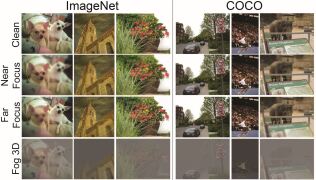
Figure 5: 3DCC can be applied to most datasets, even those that do not come with 3D information. Several query images from the ImageNet [12] and COCO [39] dataset are shown with near focus, far focus and fog 3D corruptions applied. Notice how the objects in the circled regions go from sharp to blurry depending on the focus region and scene geometry. To get the depth information needed to create these corruptions, predictions from MiDaS [55] model is used. This gives a good enough approximation to generate realistic corruptions (as we will quantify in Sec. 5.2.4).

5.1 Preliminaries

Evaluation Tasks: 3DCC can be applied to any dataset, irrespective of the target task, e.g. dense regression or low-dimensional classification. Here we mainly experiment with surface normals and depth estimation as target tasks widely employed by the community. We note that the robustness of models solving such tasks is underexplored compared to classification tasks (See Sec. 5.2.5 for results on panoptic segmentation and object recognition). To evaluate robustness, we compute the $\ell_{1}$ error between predicted and ground truth images.

Training Details: We train UNet [59] and DPT [54] models on Taskonomy [84] using learning rate $5\times 10^{-4}$ and weight decay $2\times 10^{-6}$. We optimize the likelihood loss with Laplacian prior using AMSGrad [56], following [79]. Unless specified, all the models use the same UNet backbone (e.g. Fig. 6). We also experiment with DPT models trained on Omnidata [17] that mixes a diverse set of training datasets. Following [17], we train with learning rate $1\times 10^{-5}$, weight decay $2\times 10^{-6}$ with angular & $\ell_{1}$ losses.

Robustness mechanisms evaluated: We evaluate several popular data augmentation strategies: DeepAugment [26], style augmentation [24], and adversarial training [36]. We also include Cross-Domain Ensembles (X-DE) [79] that has been recently shown to improve robustness to corruptions by creating diverse ensemble components via input transformations. We refer to the supplementary for training details. Finally, we train a model with augmentation with corruptions from 2DCC [27] (2DCC augmentation), and another model with 3D data augmentation on top of that (2DCC + 3D augmentation).

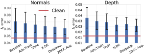
Figure 6: Existing robustness mechanisms are found to be insufficient for addressing real-world corruptions approximated by 3DCC. Performance of models with different robustness mechanisms under 3DCC for surface normals (left) and depth (right) estimation tasks are shown. All models here are UNets and are trained with Taskonomy data. Each bar shows the $\ell_{1}$ error averaged over all 3DCC corruptions (lower is better). The black error bars show the error at the lowest and highest shift intensity. The red line denotes the performance of the baseline model on clean (uncorrupted) data. This denotes that existing robustness mechanisms, including those with diverse augmentations, perform poorly under 3DCC.

5.2 3D Common Corruptions Benchmark

5.2.1 3DCC can expose vulnerabilities

We perform a benchmarking of the existing models against 3DCC to understand their vulnerabilities. However, we note that our main contribution is not the performed analyses but the benchmark itself. The state-of-the-art models may change over time and 3DCC aims to identify the robustness trends, similar to other benchmarks.

Effect of robustness mechanisms: Figure 6 shows the average performance of different robustness mechanisms on 3DCC for surface normals and depth estimation tasks. These mechanisms improved the performance over the baseline but are still far from the performance on clean data. This suggests that 3DCC exposes robustness issues and can serve as a challenging testbed for models. The 2DCC augmentation model returns slightly lower $\ell_{1}$ error, indicating that diverse 2D data augmentation only partially helps against 3D corruptions.

Effect of dataset and architecture: We provide a detailed breakdown of performance against 3DCC in Fig. 7. We first observe that baseline UNet and DPT models trained on Taskonomy have similar performance, especially on the view change corruptions. By training with larger and more diverse data with Omnidata, the DPT performance improves. Similar observations were made on vision transformers for classification [16, 5]. This improvement is notable with view change corruptions, while for the other corruptions, there is a decrease in error from 0.069 to 0.061. This suggests that combining architectural advancements with diverse and large training data can play an important role in robustness against 3DCC. Furthermore, when combined with 3D augmentations, they improve robustness to real-world corruptions (Sec. 5.3).

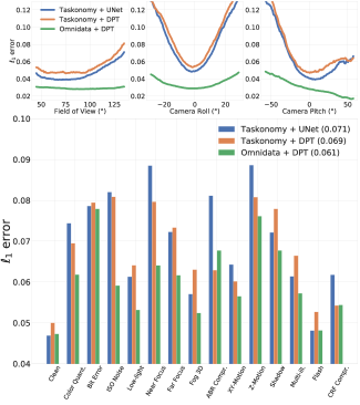
Figure 7: Detailed breakdown of performance on 3DCC. The benchmark can expose trends and models’ sensitivity to a wide range of corruptions. We show this by training models on either Taskonomy [84] or Omnidata [17] and with either a UNet [59] or DPT [54] architecture. The average $\ell_{1}$ error over all shift intensities for each corruption is shown (lower is better). Top: We observe that Taskonomy models are more susceptible to changes in field of view, camera roll, and pitch compared to Omnidata trained model, which is consistent with their methods. Bottom: The numbers in the legend are the average performance over all the corruptions. We can see that all the models are sensitive to 3D corruptions, e.g. z-motion blur and shadow. Overall, training with large diverse data, e.g. Omnidata, and using DPT is observed to notably improve performance.

Figure 8: Redundancy among corruptions. We quantified the pairwise similarity of a subset of corruptions from 2DCC and 3DCC by computing their correlations in the $\ell_{1}$ errors of the surface normals predictions (left) and RGB images (right). 3DCC incurs less correlations both intra-benchmark as well as against 2DCC. Thus, 3DCC has a diverse set of corruptions and these corruptions do not have a significant overlap with 2DCC. Using depth as target task yields similar conclusions (full affinity matrices are provided in the supplementary).

5.2.2 Redundancy of corruptions in 3DCC and 2DCC

In Fig. 1, a qualitative comparison was made between 3DCC and 2DCC. The former generates more realistic corruptions while the latter does not take scene 3D into account and applies uniform modifications over the image. In Fig. 8, we aim to quantify the similarity between 3DCC and 2DCC. On the left of Fig. 8, we compute the correlations of $\ell_{1}$ errors between clean and corrupted predictions made by the baseline model for a subset of corruptions (full set is in supplementary). 3DCC incurs less correlations both intra-benchmark as well as against 2DCC (Mean correlations are $0.32$ for 2DCC-2DCC, $0.28$ for 3DCC-3DCC, and $0.30$ for 2DCC-3DCC). Similar conclusions are obtained for depth estimation (in the supplementary). In the right, we provide the same analysis on the RGB domain by computing the $\ell_{1}$ error between clean and corrupted images, again suggesting that 3DCC yields lower correlations.

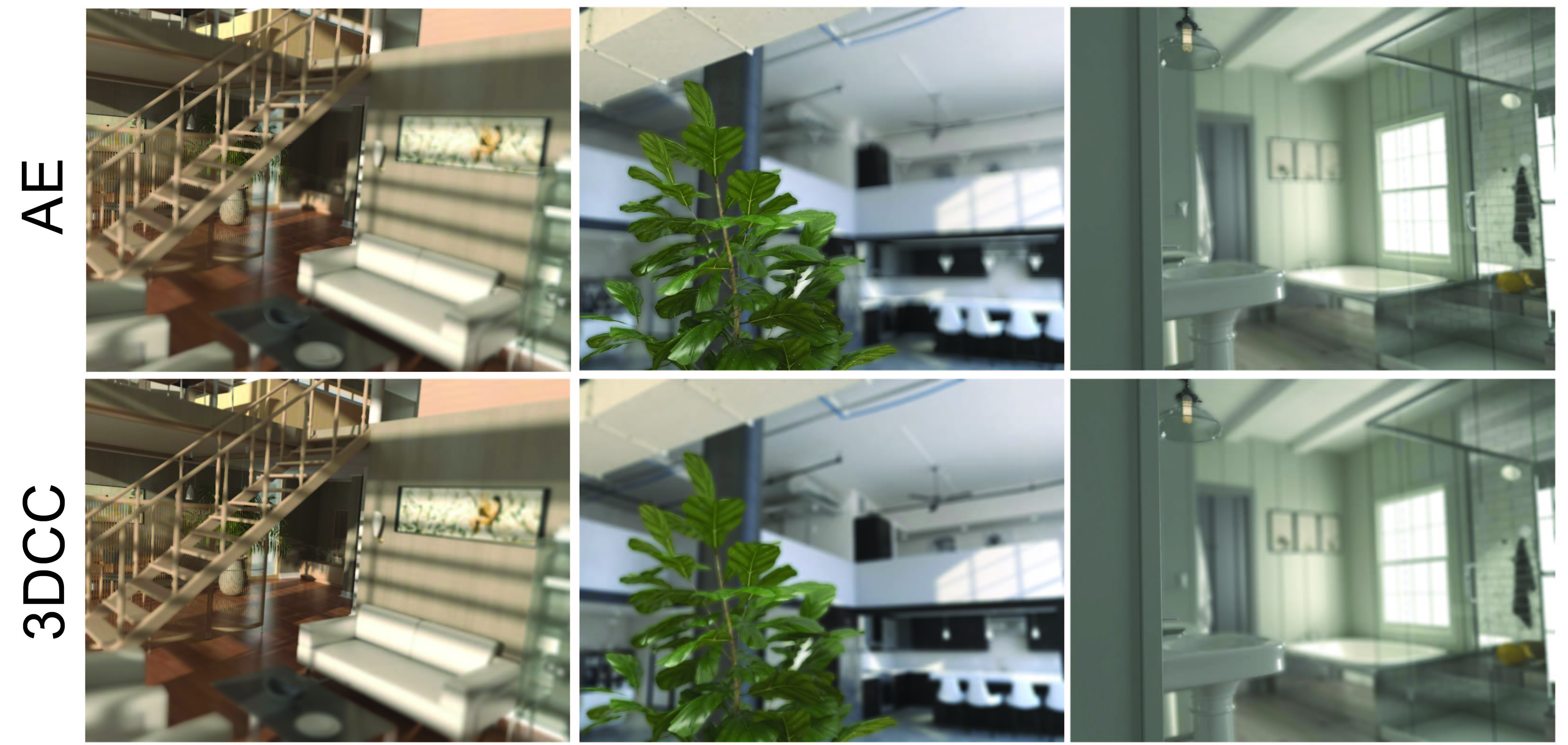
Figure 9: Visual comparisons of 3DCC and expensive After Effects (AE) generated depth of field effect on query images from Hypersim. 3DCC generated corruptions are visually similar to those from AE.

5.2.3 Soundness: 3DCC vs Expensive Synthesis

3DCC aims to expose a model’s vulnerabilities to certain real-world corruptions. This requires the corruptions generated by 3DCC to be similar to real corrupted data. As generating such labeled data is expensive and scarcely available, as a proxy evaluation, we instead compare the realism of 3DCC to synthesis made by Adobe After Effects (AE) which is a commercial product to generate high-quality photorealistic data and often relies on expensive and manual processes. To achieve this, we use the Hypersim [58] dataset that comes with high-resolution z-depth labels. We then generated 200 images that are near- and far-focused using 3DCC and AE. Figure 9 shows sample generated images from both approaches that are perceptually similar. Next, we computed the prediction errors of a baseline normal model when the input is from 3DCC or AE. The scatter plot of $\ell_{1}$ errors are given in Fig. 10 and demonstrates a strong correlation, 0.80, between the two approaches. For calibration and control, we also provide the scatter plots for some corruptions from 2DCC to show the significance of correlations. They have significantly lower correlations with AE, indicating the depth of field effect created via 3DCC matches AE generated data reasonably well.

5.2.4 Effectiveness of applying 3DCC to other datasets

We showed qualitatively in Fig. 5 that 3DCC can be applied to standard vision datasets like ImageNet [12] and COCO [39] by leveraging predicted depth from a state-of-the-art model from MiDaS [55]. Here, we quantitatively show the impact of using predicted depth instead of ground truth. For this, we use the Replica [65] dataset that comes with ground truth depth labels. We then generated 1280 corrupted images using ground truth depth and predicted depth from MiDaS [55] without fine-tuning on Replica. Figure 11 shows the trends on three corruptions from 3DCC generated using ground truth and predicted depth. The trends are similar and the correlation of errors is strong ($0.79$). This suggests that the predicted depth can be effectively used to apply 3DCC to other datasets, and the performance is expected to improve with better depth predictions.

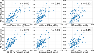
Figure 10: Corruptions of 3DCC are similar to expensive realistic synthetic ones while being cheaper to generate. Scatter plots of $\ell_{1}$ errors from the baseline model predictions on 3DCC against those created by Adobe After Effects (AE). The correlation between 3DCC near (far) focus and those from AE near (far) focus is the strongest (numbers are in the legend of left column). We also added the most similar corruption from 2DCC (defocus blur) for comparison, yielding weaker correlations (middle). Shot noise (right) is a control baseline, i.e. a randomly selected corruption, to calibrate the significance of the correlation measure.

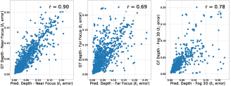
Figure 11: Effectiveness of applying 3DCC without ground truth depth. Three corruptions from 3DCC are generated using depth predictions from MiDaS [55] model on unseen Replica data. Scatter plots show the $\ell_{1}$ errors from the baseline model when corruptions are generated using the predicted depth (x-axis) or the ground truth (y-axis). The trends are similar between two corrupted data results, suggesting the predicted depth is an effective approximation to generate 3DCC. See the supplementary for more tests including control baselines.

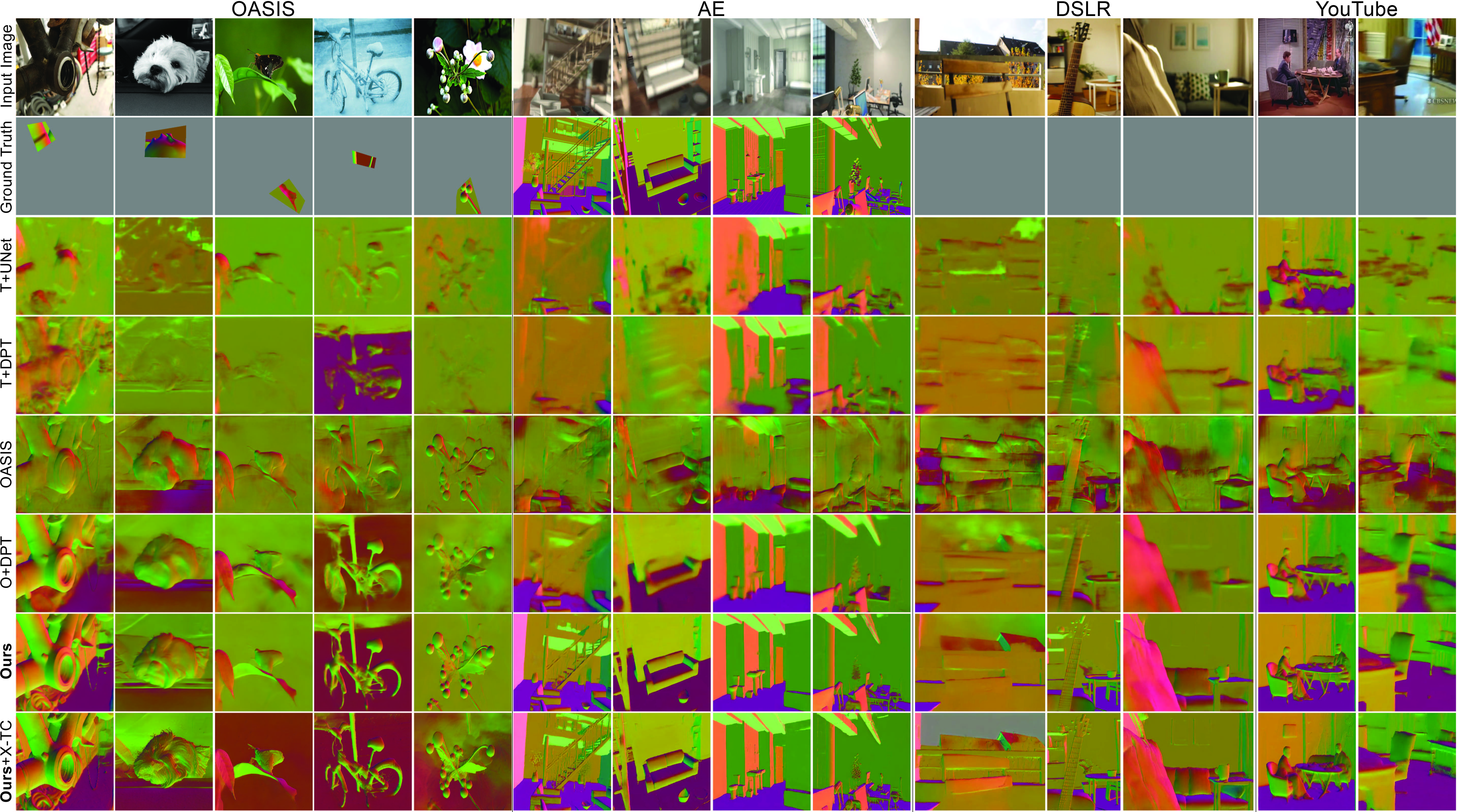
Figure 12: Qualitative results of learning with 3D data augmentation on random queries from OASIS [9], AE (Sec. 5.2.3), manually collected DSLR data, and in-the-wild YouTube videos for surface normals. The ground truth is gray when it is not available, e.g. for YouTube. The predictions in the last two rows are from the O+DPT+2DCC+3D (Ours) model. It is further trained with cross-task consistency (X-TC) constraints [83] (Ours+X-TC). They are noticeably sharper and more accurate. See the project page and supplementary for more results. A live demo for user uploaded images is also available.

5.2.5 3DCC evaluations on semantic tasks

The previous benchmarking results were focusing on surface normals and depth estimation tasks. Here we perform a benchmarking on panoptic segmentation and object recognition tasks as additional illustrative 3DCC evaluations. In particular for panoptic segmentation, we use semantic corruptions from Sec. 3.1, and for object classification, we introduce ImageNet-3DCC by applying corruptions from 3DCC to ImageNet validation set, similar to 2DCC [27].

Semantic corruptions: We evaluate the robustness of two panoptic segmentation models from [17] against occlusion corruption of 3DCC. The models are trained on Omnidata [17] and Taskonomy [84] datasets with a Detectron [75] backbone. See the supplementary for details.

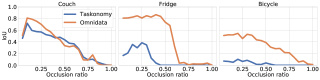
Figure 13: Robustness against occlusion corruption of 3DCC. The plot shows the intersection over union (IoU) scores of Detectron models [75] for different objects over a range of occlusion ratios. The models are trained on Taskonomy [84] or Omnidata [17] datasets. The occlusion ratio is defined as the number of occluded pixels divided by the sum of occluded and visible pixels of the object. This is computed over the test scenes of Replica [65]. The plots expose the occlusion handling capabilities of the models and show that the Omnidata trained model is generally more robust than the Taskonomy one. The degradation in model predictions is class-specific and becomes more severe with higher occlusion ratios.

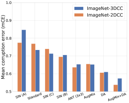
Figure 14: Robustness on ImageNet-3DCC and ImageNet-2DCC. Errors on ImageNet validation images corrupted by 3DCC and 2DCC are computed for the models in robustness leaderboards [27, 11]. Following [27], we compute the mean corruption error (mCE) relative to AlexNet [34]. The performance degrades significantly against ImageNet-3DCC, thus it can serve as a challenging benchmark. As expected, the general trends are similar between the two benchmarks as 2D and 3D corruptions are not completely disjoint. A similar observation was also made in [45] even when the corruptions are designed to be dissimilar to 2DCC. Still, there are notable differences that can be informative during model development by exposing trends and vulnerabilities that are not captured by 2DCC, e.g. ANT [61] has better mCE on 2DCC compared to AugMix [29], while they perform similarly on 3DCC. Likewise, combining DeepAugment [26] with AugMix improved the performance on 2DCC significantly more than 3DCC. See the supplementary for more results.

Figure 13 quantifies the effect of occlusion on the predictions of models, i.e. how the models’ intersection over union (IoU) scores change with increasing occlusion, for selected objects. This is computed on the test scenes from Replica [65]. The Omnidata trained model is generally more robust than the Taskonomy one, though we see a decrease in IoU in both models as occlusion increases. The trends are class-specific possibly due to shape of the objects and their scene context, e.g. fridge predictions remain unchanged up until $0.50$ occlusion ratio, while couch predictions degrade more linearly for Omnidata model. This evaluation showcases one use of semantic corruptions in 3DCC, which are notably harder to accomplish using other benchmarks that do not operate based on 3D scans.

ImageNet-3DCC: We compare performances of the robust ImageNet models [24, 61, 29, 26] from RobustBench [11] and ImageNet-2DCC [27] (i.e. ImageNet-C) leaderboards in Fig. 14. Following 2DCC, we compute mean corruption error (mCE) by dividing the models errors by AlexNet [34] errors and averaging over corruptions. The performance of models degrade significantly, including those with diverse augmentations. Thus, ImageNet-3DCC can serve as a challenging benchmark for object recognition task. As expected, while the general trends are similar between the two benchmarks as 2D and 3D corruptions are not completely disjoint [45], 3DCC exposes vulnerabilities that are not captured by 2DCC, which can be informative during model development. See supplementary for further results.

5.3 3D data augmentation to improve robustness

We demonstrate the effectiveness of the proposed augmentations qualitatively and quantitatively. We evaluate UNet and DPT models trained on Taskonomy (T+UNet, T+DPT) and DPT trained on Omnidata (O+DPT) to see the effect of training dataset and model architecture. The training procedure is as described in Sec. 5.1. For the other models, we initialize from O+DPT model and train with 2DCC augmentations (O+DPT+2DCC) and 3D augmentations on top of that (O+DPT+2DCC+3D), i.e. our proposed model. We also further trained the proposed model using cross-task consistency (X-TC) constraints from [83], denoted as (Ours+X-TC) in the results. Lastly, we evaluated a model trained on OASIS training data from [9] (OASIS).

Qualitative evaluations: We consider i. OASIS validation images [9], ii. AE corrupted data from Sec. 5.2.3, iii. manually collected DSLR data, and iv. in-the-wild YouTube videos. Figure 12 shows that predictions made by the proposed models are significantly more robust compared to baselines. We also recommend watching the clips and running the live demo on the project page.

Quantitative evaluations: In Table 1, we compute errors made by the models on 2DCC, 3DCC, AE, and OASIS validation set (no fine-tuning). Again, the proposed models yield lower errors across datasets showing the effectiveness of augmentations. Note that robustness against corrupted data is improved without sacrificing performance on in-the-wild clean data, i.e. OASIS.

T+UNet T+DPT OASIS [9] O+DPT O+DPT+2DCC Ours Ours+X-TC [83] 2DCC [27] ($\ell_{1}$ error) 8.15 7.47 15.31 6.43 5.78 5.32 5.29 3DCC ($\ell_{1}$ error) 7.08 6.89 15.11 6.13 5.94 5.42 5.35 AE (Sec. 5.2.3) ($\ell_{1}$ error) 12.86 12.39 16.85 7.84 6.50 4.94 5.47 OASIS [9] (angular error) 30.49 32.13 24.63 24.42 23.67 24.65 23.89

Table 1: Effectiveness of 3D augmentations quantified using different benchmarks. $\ell_{1}$ errors are multiplied by $100$ for readability. The O+DPT+2DCC+3D model is denoted by Ours. We also trained this model using cross-task consistency (X-TC) constraints from [83] (Ours+X-TC). Our models yield lower errors across the benchmarks. 2DCC and 3DCC are applied on the same Taskonomy test images. More results are given in supplementary. Evaluations on OASIS dataset sometimes show a large variance due to its sparse ground truth.

6 Conclusion and Limitations

We introduce a framework to test and improve model robustness against real-world distribution shifts, particularly those centered around 3D. Experiments demonstrate that the proposed 3D Common Corruptions is a challenging benchmark that exposes model vulnerabilities under real-world plausible corruptions. Furthermore, the proposed data augmentation leads to more robust predictions compared to baselines. We believe this work opens up a promising direction in robustness research by showing the usefulness of 3D corruptions in benchmarking and training. Below we briefly discuss some of the limitations:

• 3D quality: 3DCC is upper-bounded by the quality of 3D data. The current 3DCC is an imperfect but useful approximation of real-world 3D corruptions, as we showed. The fidelity is expected to improve with higher resolution sensory data and better depth prediction models.

• Non-exhaustive set: Our set of 3D corruptions and augmentations are not exhaustive. They instead serve as a starter set for researchers to experiment with. The framework can be employed to generate more domain-specific distribution shifts with minimal manual effort.

• Large-scale evaluation: While we evaluate some recent robustness approaches in our analyses, our main goal was to show that 3DCC successfully exposes vulnerabilities. Thus, performing a comprehensive robustness analysis is beyond the scope of this work. We encourage researchers to test their models against our corruptions.

• Balancing the benchmark: We did not explicitly balance the corruption types in our benchmark, e.g. having the same number of noise and blur distortions. Our work can further benefit from weighting strategies trying to calibrate average performance on corruption benchmarks, such as [37].

• Use cases of augmentations: While we focus on robustness, investigating their usefulness on other applications, e.g. self-supervised learning, could be worthwhile.

• Evaluation tasks: We experiment with dense regression tasks. However, 3DCC can be applied to different tasks, including classification and other semantic ones. Investigating failure cases of semantic models against, e.g. on smoothly changing occlusion rates for several objects, using our framework could provide useful insights.

Acknowledgement: We thank Zeynep Kar and Abhijeet Jagdev. This work was partially supported by the ETH4D and EPFL EssentialTech Centre Humanitarian Action Challenge Grant.

References

- [1] Abdelrahman Abdelhamed, Stephen Lin, and Michael S Brown. A high-quality denoising dataset for smartphone cameras. In Proceedings of the IEEE Conference on Computer Vision and Pattern Recognition, pages 1692–1700, 2018.
- [2] Iro Armeni, Zhi-Yang He, JunYoung Gwak, Amir R Zamir, Martin Fischer, Jitendra Malik, and Silvio Savarese. 3d scene graph: A structure for unified semantics, 3d space, and camera. In Proceedings of the IEEE/CVF International Conference on Computer Vision, pages 5664–5673, 2019.
- [3] Andrei Barbu, David Mayo, Julian Alverio, William Luo, Christopher Wang, Danny Gutfreund, Joshua Tenenbaum, and Boris Katz. Objectnet: A large-scale bias-controlled dataset for pushing the limits of object recognition models. 2019.
- [4] Brian A Barsky and Todd J Kosloff. Algorithms for rendering depth of field effects in computer graphics. In Proceedings of the 12th WSEAS international conference on Computers, volume 2008. World Scientific and Engineering Academy and Society (WSEAS), 2008.
- [5] Srinadh Bhojanapalli, Ayan Chakrabarti, Daniel Glasner, Daliang Li, Thomas Unterthiner, and Andreas Veit. Understanding robustness of transformers for image classification. arXiv preprint arXiv:2103.14586, 2021.
- [6] Tim Brooks and Jonathan T Barron. Learning to synthesize motion blur. In Proceedings of the IEEE/CVF Conference on Computer Vision and Pattern Recognition, pages 6840–6848, 2019.
- [7] Prithvijit Chattopadhyay, Judy Hoffman, Roozbeh Mottaghi, and Aniruddha Kembhavi. Robustnav: Towards benchmarking robustness in embodied navigation. arXiv preprint arXiv:2106.04531, 2021.
- [8] Chen Chen, Qifeng Chen, Jia Xu, and Vladlen Koltun. Learning to see in the dark. In Proceedings of the IEEE Conference on Computer Vision and Pattern Recognition, pages 3291–3300, 2018.
- [9] Weifeng Chen, Shengyi Qian, David Fan, Noriyuki Kojima, Max Hamilton, and Jia Deng. Oasis: A large-scale dataset for single image 3d in the wild. In Proceedings of the IEEE/CVF Conference on Computer Vision and Pattern Recognition, pages 679–688, 2020.
- [10] Blender Online Community. Blender - a 3D modelling and rendering package. Blender Foundation, Stichting Blender Foundation, Amsterdam, 2018.
- [11] Francesco Croce, Maksym Andriushchenko, Vikash Sehwag, Edoardo Debenedetti, Nicolas Flammarion, Mung Chiang, Prateek Mittal, and Matthias Hein. Robustbench: a standardized adversarial robustness benchmark. arXiv preprint arXiv:2010.09670, 2020.
- [12] Jia Deng, Wei Dong, Richard Socher, Li-Jia Li, Kai Li, and Li Fei-Fei. Imagenet: A large-scale hierarchical image database. In 2009 IEEE Conference on Computer Vision and Pattern Recognition, pages 248–255. Ieee, 2009.
- [13] Terrance DeVries and Graham W Taylor. Improved regularization of convolutional neural networks with cutout. arXiv preprint arXiv:1708.04552, 2017.
- [14] Josip Djolonga, Jessica Yung, Michael Tschannen, Rob Romijnders, Lucas Beyer, Alexander Kolesnikov, Joan Puigcerver, Matthias Minderer, Alexander D’Amour, Dan Moldovan, et al. On robustness and transferability of convolutional neural networks. In Proceedings of the IEEE/CVF Conference on Computer Vision and Pattern Recognition, pages 16458–16468, 2021.
- [15] Samuel Dodge and Lina Karam. A study and comparison of human and deep learning recognition performance under visual distortions. In 2017 26th International Conference on Computer Communication and Networks (ICCCN), pages 1–7. IEEE, 2017.
- [16] Alexey Dosovitskiy, Lucas Beyer, Alexander Kolesnikov, Dirk Weissenborn, Xiaohua Zhai, Thomas Unterthiner, Mostafa Dehghani, Matthias Minderer, Georg Heigold, Sylvain Gelly, et al. An image is worth 16x16 words: Transformers for image recognition at scale. arXiv preprint arXiv:2010.11929, 2020.
- [17] Ainaz Eftekhar, Alexander Sax, Jitendra Malik, and Amir Zamir. Omnidata: A scalable pipeline for making multi-task mid-level vision datasets from 3d scans. In Proceedings of the IEEE/CVF International Conference on Computer Vision, pages 10786–10796, 2021.
- [18] Michael Elad and Michal Aharon. Image denoising via sparse and redundant representations over learned dictionaries. IEEE Transactions on Image processing, 15(12):3736–3745, 2006.
- [19] Raanan Fattal. Single image dehazing. ACM transactions on graphics (TOG), 27(3):1–9, 2008.
- [20] Rob Fergus, Barun Singh, Aaron Hertzmann, Sam T Roweis, and William T Freeman. Removing camera shake from a single photograph. In ACM SIGGRAPH 2006 Papers, pages 787–794. 2006.
- [21] Alessandro Foi, Mejdi Trimeche, Vladimir Katkovnik, and Karen Egiazarian. Practical poissonian-gaussian noise modeling and fitting for single-image raw-data. IEEE Transactions on Image Processing, 17(10):1737–1754, 2008.
- [22] Nic Ford, Justin Gilmer, Nicolas Carlini, and Dogus Cubuk. Adversarial examples are a natural consequence of test error in noise. arXiv preprint arXiv:1901.10513, 2019.
- [23] Robert Geirhos, Jörn-Henrik Jacobsen, Claudio Michaelis, Richard Zemel, Wieland Brendel, Matthias Bethge, and Felix A Wichmann. Shortcut learning in deep neural networks. arXiv preprint arXiv:2004.07780, 2020.
- [24] Robert Geirhos, Patricia Rubisch, Claudio Michaelis, Matthias Bethge, Felix A Wichmann, and Wieland Brendel. Imagenet-trained cnns are biased towards texture; increasing shape bias improves accuracy and robustness. arXiv preprint arXiv:1811.12231, 2018.
- [25] Majed El Helou, Ruofan Zhou, Johan Barthas, and Sabine Süsstrunk. Vidit: virtual image dataset for illumination transfer. arXiv preprint arXiv:2005.05460, 2020.
- [26] Dan Hendrycks, Steven Basart, Norman Mu, Saurav Kadavath, Frank Wang, Evan Dorundo, Rahul Desai, Tyler Zhu, Samyak Parajuli, Mike Guo, et al. The many faces of robustness: A critical analysis of out-of-distribution generalization. In Proceedings of the IEEE/CVF International Conference on Computer Vision, pages 8340–8349, 2021.
- [27] Dan Hendrycks and Thomas Dietterich. Benchmarking neural network robustness to common corruptions and perturbations. arXiv preprint arXiv:1903.12261, 2019.
- [28] Dan Hendrycks, Kimin Lee, and Mantas Mazeika. Using pre-training can improve model robustness and uncertainty. In International Conference on Machine Learning, pages 2712–2721. PMLR, 2019.
- [29] Dan Hendrycks, Norman Mu, Ekin D Cubuk, Barret Zoph, Justin Gilmer, and Balaji Lakshminarayanan. Augmix: A simple data processing method to improve robustness and uncertainty. arXiv preprint arXiv:1912.02781, 2019.
- [30] Xiaowei Hu, Chi-Wing Fu, Lei Zhu, and Pheng-Ann Heng. Depth-attentional features for single-image rain removal. In Proceedings of the IEEE/CVF Conference on Computer Vision and Pattern Recognition, pages 8022–8031, 2019.
- [31] Jason Jo and Yoshua Bengio. Measuring the tendency of cnns to learn surface statistical regularities. arXiv preprint arXiv:1711.11561, 2017.
- [32] Christoph Kamann and Carsten Rother. Benchmarking the robustness of semantic segmentation models. In Proceedings of the IEEE/CVF Conference on Computer Vision and Pattern Recognition, pages 8828–8838, 2020.
- [33] Sanjay Kariyappa and Moinuddin K Qureshi. Improving adversarial robustness of ensembles with diversity training. arXiv preprint arXiv:1901.09981, 2019.
- [34] Alex Krizhevsky, Ilya Sutskever, and Geoffrey E Hinton. Imagenet classification with deep convolutional neural networks. Advances in neural information processing systems, 25:1097–1105, 2012.
- [35] Deepa Kundur and Dimitrios Hatzinakos. Blind image deconvolution. IEEE signal processing magazine, 13(3):43–64, 1996.
- [36] Alexey Kurakin, Ian Goodfellow, and Samy Bengio. Adversarial machine learning at scale. arXiv preprint arXiv:1611.01236, 2016.
- [37] Alfred Laugros, Alice Caplier, and Matthieu Ospici. Using synthetic corruptions to measure robustness to natural distribution shifts. arXiv preprint arXiv:2107.12052, 2021.
- [38] Guillaume Leclerc, Hadi Salman, Andrew Ilyas, Sai Vemprala, Logan Engstrom, Vibhav Vineet, Kai Xiao, Pengchuan Zhang, Shibani Santurkar, Greg Yang, et al. 3db: A framework for debugging computer vision models. arXiv preprint arXiv:2106.03805, 2021.
- [39] Tsung-Yi Lin, Michael Maire, Serge Belongie, James Hays, Pietro Perona, Deva Ramanan, Piotr Dollár, and C Lawrence Zitnick. Microsoft coco: Common objects in context. In European conference on computer vision, pages 740–755. Springer, 2014.
- [40] Raphael Gontijo Lopes, Dong Yin, Ben Poole, Justin Gilmer, and Ekin D Cubuk. Improving robustness without sacrificing accuracy with patch gaussian augmentation. arXiv preprint arXiv:1906.02611, 2019.
- [41] Aleksander Madry, Aleksandar Makelov, Ludwig Schmidt, Dimitris Tsipras, and Adrian Vladu. Towards deep learning models resistant to adversarial attacks. arXiv preprint arXiv:1706.06083, 2017.
- [42] Julien Mairal, Francis Bach, Jean Ponce, Guillermo Sapiro, and Andrew Zisserman. Non-local sparse models for image restoration. In 2009 IEEE 12th International Conference on Computer Vision, pages 2272–2279. IEEE, 2009.
- [43] Claudio Michaelis, Benjamin Mitzkus, Robert Geirhos, Evgenia Rusak, Oliver Bringmann, Alexander S Ecker, Matthias Bethge, and Wieland Brendel. Benchmarking robustness in object detection: Autonomous driving when winter is coming. arXiv preprint arXiv:1907.07484, 2019.
- [44] John P Miller, Rohan Taori, Aditi Raghunathan, Shiori Sagawa, Pang Wei Koh, Vaishaal Shankar, Percy Liang, Yair Carmon, and Ludwig Schmidt. Accuracy on the line: On the strong correlation between out-of-distribution and in-distribution generalization. In International Conference on Machine Learning, pages 7721–7735. PMLR, 2021.
- [45] Eric Mintun, Alexander Kirillov, and Saining Xie. On interaction between augmentations and corruptions in natural corruption robustness. arXiv preprint arXiv:2102.11273, 2021.
- [46] Seungjun Nah, Tae Hyun Kim, and Kyoung Mu Lee. Deep multi-scale convolutional neural network for dynamic scene deblurring. In Proceedings of the IEEE Conference on Computer Vision and Pattern Recognition, pages 3883–3891, 2017.
- [47] Seungjun Nah, Sanghyun Son, Suyoung Lee, Radu Timofte, and Kyoung Mu Lee. Ntire 2021 challenge on image deblurring. In CVPR Workshops, pages 149–165, June 2021.
- [48] Muzammal Naseer, Kanchana Ranasinghe, Salman Khan, Munawar Hayat, Fahad Shahbaz Khan, and Ming-Hsuan Yang. Intriguing properties of vision transformers. arXiv preprint arXiv:2105.10497, 2021.
- [49] Simon Niklaus, Long Mai, Jimei Yang, and Feng Liu. 3d ken burns effect from a single image. ACM Transactions on Graphics (TOG), 38(6):1–15, 2019.
- [50] A Emin Orhan. Robustness properties of facebook’s resnext wsl models. arXiv preprint arXiv:1907.07640, 2019.
- [51] Tianyu Pang, Kun Xu, Chao Du, Ning Chen, and Jun Zhu. Improving adversarial robustness via promoting ensemble diversity. arXiv preprint arXiv:1901.08846, 2019.
- [52] Amandalynne Paullada, Inioluwa Deborah Raji, Emily M Bender, Emily Denton, and Alex Hanna. Data and its (dis) contents: A survey of dataset development and use in machine learning research. arXiv preprint arXiv:2012.05345, 2020.
- [53] Michael Potmesil and Indranil Chakravarty. A lens and aperture camera model for synthetic image generation. ACM SIGGRAPH Computer Graphics, 15(3):297–305, 1981.
- [54] René Ranftl, Alexey Bochkovskiy, and Vladlen Koltun. Vision transformers for dense prediction. In Proceedings of the IEEE/CVF International Conference on Computer Vision, pages 12179–12188, 2021.
- [55] René Ranftl, Katrin Lasinger, David Hafner, Konrad Schindler, and Vladlen Koltun. Towards robust monocular depth estimation: Mixing datasets for zero-shot cross-dataset transfer. arXiv preprint arXiv:1907.01341, 2019.
- [56] Sashank J Reddi, Satyen Kale, and Sanjiv Kumar. On the convergence of adam and beyond. arXiv preprint arXiv:1904.09237, 2019.
- [57] Jaesung Rim, Haeyun Lee, Jucheol Won, and Sunghyun Cho. Real-world blur dataset for learning and benchmarking deblurring algorithms. In European Conference on Computer Vision, pages 184–201. Springer, 2020.
- [58] Mike Roberts, Jason Ramapuram, Anurag Ranjan, Atulit Kumar, Miguel Angel Bautista, Nathan Paczan, Russ Webb, and Joshua M Susskind. Hypersim: A photorealistic synthetic dataset for holistic indoor scene understanding. In Proceedings of the IEEE/CVF International Conference on Computer Vision, pages 10912–10922, 2021.
- [59] Olaf Ronneberger, Philipp Fischer, and Thomas Brox. U-net: Convolutional networks for biomedical image segmentation. In International Conference on Medical Image Computing and Computer-assisted Intervention, pages 234–241. Springer, 2015.
- [60] Evgenia Rusak, Lukas Schott, Roland Zimmermann, Julian Bitterwolfb, Oliver Bringmann, Matthias Bethge, and Wieland Brendel. Increasing the robustness of dnns against image corruptions by playing the game of noise. 2020.
- [61] Evgenia Rusak, Lukas Schott, Roland S Zimmermann, Julian Bitterwolf, Oliver Bringmann, Matthias Bethge, and Wieland Brendel. A simple way to make neural networks robust against diverse image corruptions. In European Conference on Computer Vision, pages 53–69. Springer, 2020.
- [62] Christos Sakaridis, Dengxin Dai, and Luc Van Gool. Semantic foggy scene understanding with synthetic data. International Journal of Computer Vision, 126(9):973–992, 2018.
- [63] Nithya Sambasivan, Shivani Kapania, Hannah Highfill, Diana Akrong, Praveen Paritosh, and Lora M Aroyo. “everyone wants to do the model work, not the data work”: Data cascades in high-stakes ai. In Proceedings of the 2021 CHI Conference on Human Factors in Computing Systems, pages 1–15, 2021.
- [64] Rulin Shao, Zhouxing Shi, Jinfeng Yi, Pin-Yu Chen, and Cho-Jui Hsieh. On the adversarial robustness of visual transformers. arXiv preprint arXiv:2103.15670, 2021.
- [65] Julian Straub, Thomas Whelan, Lingni Ma, Yufan Chen, Erik Wijmans, Simon Green, Jakob J. Engel, Raul Mur-Artal, Carl Ren, Shobhit Verma, Anton Clarkson, Mingfei Yan, Brian Budge, Yajie Yan, Xiaqing Pan, June Yon, Yuyang Zou, Kimberly Leon, Nigel Carter, Jesus Briales, Tyler Gillingham, Elias Mueggler, Luis Pesqueira, Manolis Savva, Dhruv Batra, Hauke M. Strasdat, Renzo De Nardi, Michael Goesele, Steven Lovegrove, and Richard Newcombe. The Replica dataset: A digital replica of indoor spaces. arXiv preprint arXiv:1906.05797, 2019.
- [66] Jiachen Sun, Qingzhao Zhang, Bhavya Kailkhura, Zhiding Yu, Chaowei Xiao, and Z Morley Mao. Benchmarking robustness of 3d point cloud recognition against common corruptions. arXiv preprint arXiv:2201.12296, 2022.
- [67] Christian Szegedy, Wojciech Zaremba, Ilya Sutskever, Joan Bruna, Dumitru Erhan, Ian Goodfellow, and Rob Fergus. Intriguing properties of neural networks. arXiv preprint arXiv:1312.6199, 2013.
- [68] Rohan Taori, Achal Dave, Vaishaal Shankar, Nicholas Carlini, Benjamin Recht, and Ludwig Schmidt. Measuring robustness to natural distribution shifts in image classification. arXiv preprint arXiv:2007.00644, 2020.
- [69] Maxime Tremblay, Shirsendu Sukanta Halder, Raoul de Charette, and Jean-François Lalonde. Rain rendering for evaluating and improving robustness to bad weather. International Journal of Computer Vision, 129(2):341–360, 2021.
- [70] Alexander Von Bernuth, Georg Volk, and Oliver Bringmann. Simulating photo-realistic snow and fog on existing images for enhanced cnn training and evaluation. In 2019 IEEE Intelligent Transportation Systems Conference (ITSC), pages 41–46. IEEE, 2019.
- [71] Neal Wadhwa, Rahul Garg, David E Jacobs, Bryan E Feldman, Nori Kanazawa, Robert Carroll, Yair Movshovitz-Attias, Jonathan T Barron, Yael Pritch, and Marc Levoy. Synthetic depth-of-field with a single-camera mobile phone. ACM Transactions on Graphics (ToG), 37(4):1–13, 2018.
- [72] Lijun Wang, Xiaohui Shen, Jianming Zhang, Oliver Wang, Zhe Lin, Chih-Yao Hsieh, Sarah Kong, and Huchuan Lu. Deeplens: Shallow depth of field from a single image. arXiv preprint arXiv:1810.08100, 2018.
- [73] Zhou Wang, Alan C Bovik, Hamid R Sheikh, and Eero P Simoncelli. Image quality assessment: from error visibility to structural similarity. IEEE Transactions on Image Processing, 13(4):600–612, 2004.
- [74] Kaixuan Wei, Ying Fu, Jiaolong Yang, and Hua Huang. A physics-based noise formation model for extreme low-light raw denoising. In Proceedings of the IEEE/CVF Conference on Computer Vision and Pattern Recognition, pages 2758–2767, 2020.
- [75] Yuxin Wu, Alexander Kirillov, Francisco Massa, Wan-Yen Lo, and Ross Girshick. Detectron2. https://github.com/facebookresearch/detectron2, 2019.
- [76] Qizhe Xie, Minh-Thang Luong, Eduard Hovy, and Quoc V Le. Self-training with noisy student improves imagenet classification. In Proceedings of the IEEE/CVF Conference on Computer Vision and Pattern Recognition, pages 10687–10698, 2020.
- [77] Zexiang Xu, Kalyan Sunkavalli, Sunil Hadap, and Ravi Ramamoorthi. Deep image-based relighting from optimal sparse samples. ACM Transactions on Graphics (ToG), 37(4):1–13, 2018.
- [78] Huanrui Yang, Jingyang Zhang, Hongliang Dong, Nathan Inkawhich, Andrew Gardner, Andrew Touchet, Wesley Wilkes, Heath Berry, and Hai Li. Dverge: Diversifying vulnerabilities for enhanced robust generation of ensembles. Advances in Neural Information Processing Systems, 33, 2020.
- [79] Teresa Yeo, Oğuzhan Fatih Kar, and Amir Zamir. Robustness via cross-domain ensembles. In Proceedings of the IEEE/CVF International Conference on Computer Vision (ICCV), pages 12189–12199, October 2021.
- [80] Chenyu Yi, Siyuan Yang, Haoliang Li, Yap-peng Tan, and Alex Kot. Benchmarking the robustness of spatial-temporal models against corruptions. arXiv preprint arXiv:2110.06513, 2021.
- [81] Dong Yin, Raphael Gontijo Lopes, Jon Shlens, Ekin Dogus Cubuk, and Justin Gilmer. A fourier perspective on model robustness in computer vision. In Advances in Neural Information Processing Systems, pages 13276–13286, 2019.
- [82] Sangdoo Yun, Dongyoon Han, Seong Joon Oh, Sanghyuk Chun, Junsuk Choe, and Youngjoon Yoo. Cutmix: Regularization strategy to train strong classifiers with localizable features. In Proceedings of the IEEE/CVF International Conference on Computer Vision, pages 6023–6032, 2019.
- [83] Amir Zamir, Alexander Sax, Teresa Yeo, Oğuzhan Kar, Nikhil Cheerla, Rohan Suri, Zhangjie Cao, Jitendra Malik, and Leonidas Guibas. Robust learning through cross-task consistency. arXiv preprint arXiv:2006.04096, 2020.
- [84] Amir R Zamir, Alexander Sax, William Shen, Leonidas J Guibas, Jitendra Malik, and Silvio Savarese. Taskonomy: Disentangling task transfer learning. In Proceedings of the IEEE Conference on Computer Vision and Pattern Recognition, pages 3712–3722, 2018.
- [85] Hongyi Zhang, Moustapha Cisse, Yann N Dauphin, and David Lopez-Paz. mixup: Beyond empirical risk minimization. arXiv preprint arXiv:1710.09412, 2017.
- [86] Kai Zhang, Wangmeng Zuo, Yunjin Chen, Deyu Meng, and Lei Zhang. Beyond a gaussian denoiser: Residual learning of deep cnn for image denoising. IEEE transactions on image processing, 26(7):3142–3155, 2017.
- [87] Kai Zhang, Wangmeng Zuo, Shuhang Gu, and Lei Zhang. Learning deep cnn denoiser prior for image restoration. In Proceedings of the IEEE conference on computer vision and pattern recognition, pages 3929–3938, 2017.