Hierarchical Reinforcement Learning with AI Planning Models

Abstract

Two common approaches to sequential decision-making are AI planning (AIP) and reinforcement learning (RL). Each has strengths and weaknesses. AIP is interpretable, easy to integrate with symbolic knowledge, and often efficient, but requires an up-front logical domain specification and is sensitive to noise; RL only requires specification of rewards and is robust to noise but is sample inefficient and not easily supplied with external knowledge. We propose an integrative approach that combines high-level planning with RL, retaining interpretability, transfer, and efficiency, while allowing for robust learning of the lower-level plan actions.

Our approach defines options in hierarchical reinforcement learning (HRL) from AIP operators by establishing a correspondence between the state transition model of AI planning problem and the abstract state transition system of a Markov Decision Process (MDP). Options are learned by adding intrinsic rewards to encourage consistency between the MDP and AIP transition models. We demonstrate the benefit of our integrated approach by comparing the performance of RL and HRL algorithms in both MiniGrid and N-rooms environments, showing the advantage of our method over the existing ones.

Introduction

Sequential decision-making problems have been historically tackled with two distinct and largely complementary research paradigms: AI planning (AIP) and reinforcement learning (RL). In AIP, a human modeler creates a domain specification in logic which specifies action (operator) preconditions and effects. This approach can yield computationally efficient planning and interpretable plans, but AIP planners are not tolerant to noise or uncertainty, and specification of the domain can be difficult when it is not well-understood or complex. By contrast, model-free deep reinforcement learning approaches lift the burden of model specification, inherit the tolerance to noise and uncertainty of neural networks, and require no special human understanding of the domain. But RL does not generate easily interpretable policies and domain-specific knowledge, which can be hugely important in sample efficient learning, must be specified obliquely through the design of training algorithms, policy networks and reward structures.

HRL (Barto and Mahadevan 2003) aims to improve the sample efficiency of non-hierarchical RL methods for solving large scale problems by exploiting domain knowledge that allows decomposing task structures in the abstract state and action space (Dean and Lin 1995). Notable earlier works include hierarchical abstract machines (Parr and Russell 1998) that encode domain knowledge about high-level state transition into a finite state machine, options framework (Sutton, Precup, and Singh 1999) that characterizes HRL as executing sub-routines, each generating temporarily extended actions in semi-MDP (SMDP), and feudal RL (Dayan and Hinton 1992) that presents hierarchical control architecture, where the lower-level agents achieve subgoals directed by the higher-level control agent. Then, later works focus on discovering temporally extended actions such as options (Bacon, Harb, and Precup 2017; Machado, Bellemare, and Bowling 2017; Bagaria and Konidaris 2019), learning state abstractions (Ravindran and Barto 2004; Li, Walsh, and Littman 2006) or skills or sub-tasks (McGovern and Barto 2001; Stolle and Precup 2002; Castro and Precup 2011; Simsek and Barreto 2008). More recently, state abstraction has also been used in option learning(Abdulhai et al. 2022) to further improve the sample efficiency of HRL. In addition to infusing knowledge for decomposing the task, HRL agents could inform the lower-level control agents with intrinsic rewards (Singh, Barto, and Chentanez 2004) to better guide optimization procedure (Vezhnevets et al. 2017; Kulkarni et al. 2016; Nachum et al. 2018).

Recently, we see increasing interest in integrating symbolic methods in AIP and deep RL due to their complementary nature. Reward machines (RM) (Icarte et al. 2018) specify the reward of MDP over a finite-state machine (FSM) such that the agent can learn policies that follow the symbolic event models, encoded manually, or translated from linear temporal logic (LTL) expressions specifying possible symbolic policies (Camacho et al. 2019). Then, those FSMs augmented with symbolic knowledge can also be utilized to define temporarily extended actions for HRL agents. (Icarte et al. 2022; Araki et al. 2021; Den Hengst et al. 2022). High-level instructions for guiding RL can also be provided through a sequence of symbolic trajectories in various forms such as state predicates and action operators in AIP (Illanes et al. 2020), or other formal action languages Yang et al. (2018); Lyu et al. (2019); Kokel et al. (2021a, b).

When the problem involves complex task structures, e.g., as in combined task and motion planning (Eppe, Nguyen, and Wermter 2019; Garrett et al. 2021) or in the RL environments originated from AIP domains (Toyer et al. 2018; Groshev et al. 2018; Shen, Trevizan, and Thiébaux 2020), the integrated approach is a more natural choice, and we often have access to domain knowledge that captures the task structure for defining AIP models. In this paper, we present an integrated AI planning and RL framework for HRL, which we call Planning annotated RL (PaRL). In PaRL, we provide an AIP model annotating the RL environment, which offers abstract and partial knowledge about the RL MDP. Unlike other integrated methods, the annotating AIP model is a valid planning task that the planning agent can supply to AI planners. The main contributions of the paper are summarized as follows: (1) Unlike other approaches that require a manual process or rely on the solution to the problem, we present a method for deriving options directly from AIP model. (2) We design a method for generating intrinsic rewards for RL agents that encourages consistency between the annotating task and MDP transitions by introducing consistency constraints at the planning level. (3) We show the improvement in sample efficiency due to decomposition and additional benefits inherit from AIP and RL approaches in MiniGrid and N-rooms environments (Chevalier-Boisvert, Willems, and Pal 2018; Chevalier-Boisvert et al. 2019).

Background

RL and Options Framework

We assume that an agent interacts with a goal-oriented MDP ${\mathcal{M}}=\langle\mathcal{S},\mathcal{A},P,r,s_{0},G,\gamma\rangle$ with states $\mathcal{S}$, actions $\mathcal{A}$, a state transition function $P:\mathcal{S}\times\mathcal{A}\times\mathcal{S}\rightarrow[0,1]$, a reward function $r:\mathcal{S}\times\mathcal{A}\rightarrow\mathbb{R}$, an initial state $s_{0}\in\mathcal{S}$, a set of goal states $G\subset\mathcal{S}$, and a discounting factor $\gamma\in(0,1)$ for the rewards. In this goal-oriented environment, we are interested in the sparse reward task, and the objective is to learn a stationary optimal policy $\pi^{*}$ that maximizes the expected return, $\pi^{*}=\arg\max_{\pi}\mathbb{E}_{\pi}[\sum_{t=0}^{\infty}\gamma^{t}r_{t}|s_{0}],$ where $s_{0}$ is the initial state, and $\pi(a|s)$ is a stochastic policy $\pi:\mathcal{S}\times\mathcal{A}\rightarrow[0,1]$.

A value function $V^{\pi}(s)$ is the expected sum of the discounted reward in each state $s\in\mathcal{S}$,

$$V^{\pi}(s)\!\!=\!\!\sum_{a\in\mathcal{A}}\pi(a|s)[r(s,a)+\gamma\sum_{s^{\prime}\in\mathcal{S}}P(s^{\prime}|s,a)V^{\pi}(s^{\prime})].$$

The action-value function gives the value of executing an action $a\in\mathcal{A}$ in state $s\in\mathcal{S}$ under the policy $\pi$,

$$Q^{\pi}(s,a)=r(s,a)+\gamma\sum_{s^{\prime}\in\mathcal{S}}P(s^{\prime}|s,a)Q^{\pi}(s^{\prime}).$$

The optimal value function $V^{*}(s)$ and action-value function $Q^{*}(s,a)$ can be found by $V^{*}(s)=\max_{\pi}V^{\pi}(s)$ and $Q^{*}(s,a)=\max_{\pi}Q^{\pi}(s,a).$

In options framework (Sutton and Barto 1998), A set of options ${\cal O}$ formalizes the temporally extended actions that defines a semi-MDP (SMDP) over the original MDP ${\mathcal{M}}$. A Markovian option ${O}\in{\cal O}$ is a triple $\langle{\mathcal{I}_{{O}}},\pi_{{O}},\beta_{{O}}\rangle$, where ${\mathcal{I}_{{O}}}$ is the initiation set in which ${O}$ can begin, $\pi_{{O}}$ is a stationary option policy $\pi_{{O}}:\mathcal{S}\times\mathcal{A}\rightarrow[0,1]$, and $\beta_{{O}}$ is a termination set in which ${O}$ terminates. We follow the call-and-return option execution model, where an agent selects an option ${O}$ using an option level policy $\mu({O}|s)$ in state $s$ at time $t$, and generates a sequence of actions according to the option policy $\pi_{o}(a|s)$. The execution of an option ${O}$ continues up to $k$ steps until reaching the $\beta_{{O}}$ and it returns the option reward $R(s,{O})$ accumulated from $t+1$ to $t+k$ with a discounting factor $\gamma$,

$$R(s,{O})=\mathbb{E}\big{[}\sum_{t^{\prime}=t+1}^{t+k}\gamma^{t^{\prime}-t-1}r_{t^{\prime}}|\mathcal{E}({O},s,t)\big{]},$$

where $\mathcal{E}({O},s,t)$ denotes the event of an option ${O}$ being selected in state $s$ at time $t$, and $r_{t^{\prime}}$ denotes the reward obtained at time $t^{\prime}$. The state transition probability from a state $s$ to a state $s^{\prime}$ under the execution of an option ${O}$ can be written as

$$P(s^{\prime}|s,{O})=\sum_{j=0}^{\infty}\gamma^{j}Pr\big{(}k=j,s_{t+j}|\mathcal{E}({O},s,t)\big{)}.$$

In SMDP, the value function $V^{\mu}(s)$ under the option level policy $\mu$ can be written as

$$V^{\mu}(s)\!=\!\sum_{{O}\in{\cal O}}\mu({O}|s)\Big{[}R(s,{O})\!+\!\sum_{s^{\prime}\in\mathcal{S}}P(s^{\prime}|s,{O})V^{\mu}(s^{\prime})\Big{]},$$

and the option-value function $Q^{\mu}(s,O)$ is

$$Q^{\mu}(s,{O})\!=\!R(s,{O})\!+\!\sum_{s^{\prime}\in\mathcal{S}}\!\!P(s^{\prime}|s,{O})\sum_{{O}\in{\cal O}}\!\!\mu({O}|s)Q^{\mu}(s^{\prime},{O}).$$

In general, learning options ranges from the offline option discovery to the online end-to-end option critic approach (Bacon, Harb, and Precup 2017), and each option policy $\pi_{{\cal O}}$ could be trained by existing RL algorithms such as value-based methods or policy-gradient methods. Given a set of learned options ${\cal O}$, an off-policy learning methods such as Q-learning (Watkins and Dayan 1992; Mnih et al. 2015) can learn the option value function by SMDP Q-learning (Sutton, Precup, and Singh 1999).

AI Planning

To formally represent planning tasks, we follow the notation of $\textsc{sas}^{+}$ planning tasks (Bäckström and Nebel 1995). In $\textsc{sas}^{+}$, a planning task $\Pi$ is given by a tuple $\langle\mathcal{V},\mathcal{O},s_{0}^{\prime},s_{\ast}\rangle$, where $\mathcal{V}$ is a finite set of state variables, and $\mathcal{O}$ is a finite set of operators. Each state variable $v\in\mathcal{V}$ has a finite domain $\mathit{dom}(v)$ of values. A pair $\langle v,\vartheta\rangle$ with $v\in\mathcal{V}$ and $\vartheta\in\mathit{dom}(v)$ is called a fact. A (partial) assignment to $\mathcal{V}$ is called a (partial) state, with the full state $s_{0}^{\prime}$ being the initial state and the partial state $s_{\ast}$ being the goal. We denote the variables of a partial assignment $p$ by $\mathcal{V}(p)$. It is convenient to view a partial state $p$ as a set of facts with $\langle v,\vartheta\rangle\in p$ if and only if $p[v]=\vartheta$. A partial state $p$ is consistent with state $s$ if $p\subseteq s$.

We denote the set of states of $\Pi$ by $\mathcal{S}^{\prime}$. Each operator $o\!\in\!\mathcal{O}$ is a pair $\langle\textit{pre}(o),\mathit{eff}(o)\rangle$ of partial states called preconditions and effects. The (possibly empty) subset of preconditions that do not involve variables from the effect is called prevail condition, $\textit{prv}(o)\!=\!\{\langle\!v,\vartheta\!\rangle\!\mid\!\langle v,\vartheta\rangle\!\in\!\textit{pre}(o),v\not\in\mathcal{V}(\mathit{eff}(o))\}$. An operator $o$ is applicable in a state $s\in\mathcal{S}^{\prime}$ if and only if $\textit{pre}(o)$ is consistent with $s$ ($\textit{pre}(o)\subseteq s$). Applying $o$ changes the value of $v$ to $\mathit{eff}(o)[v]$, if defined. The resulting state is denoted by $s\llbracket o\rrbracket$. An operator sequence $\pi=\langle o_{1},\dots,o_{k}\rangle$ is applicable in $s$ if there exist states $s_{0},\cdots,s_{k}$ such that (1) $s_{0}=s$, and (2) for each $1\leq i\leq k$, $\textit{pre}(o_{i})\subset s_{i\mbox{-}1}$ and $s_{i}=s_{i\mbox{-}1}\llbracket o_{i}\rrbracket$. We denote the state $s_{k}$ by $s\llbracket\pi\rrbracket$. $\pi$ is a plan for $s$ iff $\pi$ is applicable in $s$ and $s_{\ast}\subseteq s\llbracket\pi\rrbracket$.

A transition graph of a planning task $\Pi=\langle\mathcal{V},\mathcal{O},s_{0}^{\prime},s_{\ast}\rangle$ is a triple ${\cal T}_{\Pi}=\langle\mathcal{S},T_{\Pi},s_{\ast}\rangle$, where $\mathcal{S}$ are the states of $\Pi$, $T_{\Pi}\subseteq\mathcal{S}\times\mathcal{O}\times\mathcal{S}$ is a set of labeled transitions, and $s_{\ast}\subseteq\mathcal{S}$ is the set of goal states. An abstraction of the transition graph ${\cal T}$ is a pair $\langle{\cal T}^{\prime},\alpha\rangle$, where ${\cal T}^{\prime}=\langle\mathcal{S}^{\prime},T^{\prime},\mathcal{S}_{\ast}^{\prime}\rangle$ is an abstract transition graph and $\alpha:\mathcal{S}\mapsto\mathcal{S}^{\prime}$ is an abstraction mapping, such that $\langle\alpha(s),o,\alpha(s^{\prime})\rangle\in T^{\prime}$ for all $\langle s,o,s^{\prime}\rangle\in T$, and $\alpha(s)\in\mathcal{S}_{\ast}^{\prime}$ for all $s\in\mathcal{S}_{\ast}$.

Annotating RL with Planning

In this section, we formulate our HRL framework. The basic idea is to link the AI planning task and the MDP task by viewing the former as an abstraction of the latter and mapping all transitions associated with a planning operator to a temporal abstraction encapsulated in the RL option (Sutton, Precup, and Singh 1999).

PaRL Task

We start by defining a Planning annotated RL (PaRL) task and present the options framework derived from a symbolic planning task.

Definition 1

A PaRL task is a triple $E:=\langle{\mathcal{M}},\Pi,L\rangle$, where ${\mathcal{M}}:=\langle\mathcal{S},\mathcal{A},P,r,s_{0},G,\gamma\rangle$ is a goal-oriented MDP over states $\mathcal{S}$, $\Pi:=\langle\mathcal{V},\mathcal{O},s_{0}^{\prime},s_{\ast}\rangle$ is a planning task over states $\mathcal{S}^{\prime}$, and $L:\mathcal{S}\mapsto\mathcal{S}^{\prime}$ is a surjective mapping from the MDP states $\mathcal{S}$ to planning task states $\mathcal{S}^{\prime}$ satisfying $s_{0}^{\prime}=L(s_{0})$ and $s_{\ast}$ consistent with $L(s)$ for all $s\!\!\in\!\!G$. We denote the pre-image of $s^{\prime}\!\!\in\!\!\mathcal{S}^{\prime}$ under $L$, $\{s\!\!\in\!\!\mathcal{S}\!\!\mid\!\!L(s)\!\!=\!\!s^{\prime}\}$ by $L^{-1}(s^{\prime})$.

The generic definition of PaRL task is a mixed blessing. On the one hand, it does not pose any constraints on the connection between ${\mathcal{M}}$ and $\Pi$ beyond the consistency of the initial state and the goal under $L$. On the other hand, if the two tasks are unrelated, it is not clear what is the benefit of connecting these tasks together. We formulate the connection by extending the definition of abstraction to PaRL tasks.

Definition 2

Let $E=\langle{\mathcal{M}},\Pi,L\rangle$ be a PaRL task and ${\cal T}_{\Pi}=\langle\mathcal{S}^{\prime},T_{\Pi},S_{\ast}\rangle$ be the transition graph of $\Pi$. We say that $\langle\Pi,L\rangle$ is an abstraction of ${\mathcal{M}}$ if for all $\langle s,a,t\rangle$ we have $P(t|s,a)>0$, iff $\langle L(s),o,L(t)\rangle\in T_{\Pi}$ for some $o\in\mathcal{O}$ or $L(s)=L(t)$. We call such PaRL tasks proper.

The idea behind the definition of PaRL task is to allow the specification of some of the functionality of the reinforcement learning task in a declarative way. In what follows, we only consider proper PaRL tasks. Next, we link the RL task ${\mathcal{M}}$ and the planning task $\Pi$ by an options framework.

Definition 3

For a PaRL task $E\!:=\!\langle{\mathcal{M}},\!\Pi,\!L\rangle$, plan options are: (1) for each operator $o\!\in\!\mathcal{O}$ in $\Pi$, an operator option ${O}_{o}\!:=\!\langle{\mathcal{I}_{{O}_{o}}},\!\pi_{{O}_{o}},\!\beta_{{O}_{o}}\rangle$ with ${\mathcal{I}_{{O}_{o}}}\!:=\!\{\!s\!\in\!\mathcal{S}\!\!\mid\!\!\textit{pre}(o)\!\subseteq\!L(s)\}$ and $\beta_{{O}_{o}}:=\{s\in\mathcal{S}\mid(\textit{prv}(o)\cup\mathit{eff}(o))\subseteq L(s)\}$, and (2) a single goal option ${O}_{\ast}:=\langle{\mathcal{I}_{{O}_{\ast}}},\pi_{{O}_{\ast}},\beta_{{O}_{\ast}}\rangle$ with ${\mathcal{I}_{{O}_{\ast}}}:=\{s\in\mathcal{S}\mid s_{\ast}\subset L(s)\}$ and $\beta_{{O}_{\ast}}\!:=\!G$.

Previous attempts in the literature have suggested utilizing planning operators to define options (Lyu et al. 2019; Illanes et al. 2020). However, earlier works assume an additional domain knowledge associating planning operators with conditions over propositional variables. Here, we do not require such additional input, relying solely on the planning task.

Denoting by ${\cal O}_{{\mathcal{M}}}$, a set of plan options induces an SMDP ${\mathcal{M}}^{\prime}:=\langle\mathcal{S},{\cal O}_{{\mathcal{M}}},P,r,S_{0},G,\gamma\rangle$, where we replace the primitive actions $\mathcal{A}$ in ${\mathcal{M}}$ with ${\cal O}_{{\mathcal{M}}}$. Next, we define a transition graph ${\cal T}_{{\mathcal{M}}^{\prime}}$ of ${\mathcal{M}}^{\prime}$ in which a multi-step state transition of an option ${O}_{o}$ is collapsed to a single labeled transition that connects each state $s\in{\mathcal{I}_{{O}_{o}}}$ to the states $t\in\beta_{{O}_{o}}$.

Definition 4

Given a PaRL task $E:=\langle{\mathcal{M}},\Pi,L\rangle$, a transition graph of the SMDP ${\mathcal{M}}^{\prime}:=\langle\mathcal{S},{\cal O}_{{\mathcal{M}}},P,r,s_{0},G,\gamma\rangle$ is a triple ${\cal T}_{{\mathcal{M}}^{\prime}}:=\langle\mathcal{S},T_{{\mathcal{M}}^{\prime}},G\rangle$, where $\mathcal{S}$ is the states of ${\mathcal{M}}$, $T_{{\mathcal{M}}^{\prime}}$ is a set of non-deterministic labeled transitions $\{\langle s,o,t\rangle\mid s\in{\mathcal{I}_{{O}_{o}}},t\in\beta_{{O}_{o}},P(t|s,{O}_{o})>0\}$, and $G$ is the goal states in ${\mathcal{M}}$.

Frames and Decompositions in Plan Options

Although we do not assume to have an exact model of ${\mathcal{M}}$, it is desirable to have an annotating planning task $\Pi$ that behaves similar to ${\mathcal{M}}$. To characterize the similarity between the two tasks, we introduce a context and frame of an option ${O}_{o}$ in an RL state $s$ to capture the subset of facts in the planning task that prevail when applying a planning operator $o$ to the planning state $L(s)$, namely $L(s)\cap L(s)\llbracket o\rrbracket$.

Definition 5

For an operator $o$ and its option ${O}_{o}$, we define the context of an operator option in state $s\in\mathcal{S}$ by $\mathcal{C}_{{O}_{o}}(s):=L(s)\setminus(\textit{pre}(o)\cup\mathit{eff}(o))$. The frame of an operator option in state $s\in\mathcal{S}$ is $\mathcal{F}_{{O}_{o}}(s):=\textit{prv}(o)\cup\mathcal{C}_{{O}_{o}}(s)$. A partial frame of an option in $s$ $\mathcal{F}^{p}_{{O}_{o}}(s)$ is a subset of $\mathcal{F}_{{O}_{o}}(s)$.

We say that a PaRL task $E$ with a set of plan options ${\cal O}_{{\mathcal{M}}}$ is frame preserving if $\mathcal{F}_{{O}_{o}}(s)=\mathcal{F}_{{O}_{o}}(t)$ for every $\langle s,o,t\rangle\in T_{{\mathcal{M}}^{\prime}}$ and operator $o\in\mathcal{O}$.

Theorem 1

If a PaRL task $E$ with plan options ${\cal O}_{{\mathcal{M}}}$ is frame preserving, then ${\cal T}_{\Pi}$ and ${\cal T}_{{\mathcal{M}}^{\prime}}$ are bisimilar.

Proof: Consider a binary relation $\{\langle s,t\rangle\!\!\in\!\!\mathcal{S}\!\times\!\mathcal{S}\!\mid\!L(s)\!\!=\!\!L(t)\}$. For each $o\in\mathcal{O}$, every $\langle s,o,t\rangle\in T_{{\mathcal{M}}^{\prime}}$ satisfies $L(t)\!\!=\!\!\big{[}L(s)\setminus\!\big{(}\textit{pre}(o)\!\cup\!\mathcal{F}_{{O}_{o}}(s)\big{)}\big{]}\cup\big{(}\mathit{eff}(o)\!\cup\!\mathcal{F}_{{O}_{o}}(s)\big{)}\!=\!L(s)\llbracket o\rrbracket.$ For a transition $\langle t,o,t^{\prime}\rangle\in T_{{\mathcal{M}}^{\prime}}$ such that $L(t)=L(s)$, $L(t^{\prime})=L(t)\llbracket o\rrbracket=L(s)\llbracket o\rrbracket$.  

The desiderata in HRL is that a task hierarchy in ${\mathcal{M}}$ captures the decomposition into sub-MDP tasks that are easier to solve in a local state space, and those sub-tasks are reusable in similar problems. It is often claimed that HRL improves sample efficiency, and a sub-problem analysis by Wen et al. (2020) shows that HRL methods can improve the sample efficiency if the total sum of the size of each partitioned state space is smaller than the size of the original state space. Following this intuition behind the MDP decomposition in HRL, we now characterize the sub-problem decomposition imposed by the frame-constrained option MDPs.

Definition 6

Given a PaRL task $E\!\!:=\!\!\langle{\mathcal{M}},\Pi,L\rangle$ and a plan option ${O}_{o}\!\!:=\!\!\langle{\mathcal{I}_{{O}_{o}}},\!\pi_{{O}_{o}},\!\beta_{{O}_{o}}\rangle$, a frame constrained option MDP is an MDP for a Markovian option ${O}_{o}$, defined as

$${\mathcal{M}}_{o,s_{0}}:=\langle\mathcal{S}_{\mathcal{F}_{o}(s_{0})},\mathcal{A},P_{\mathcal{F}_{o}(s_{0})},r,s_{0},\beta_{{O}_{o}},\mathcal{D}_{\mathcal{F}_{o}(s_{0})},\gamma\rangle,$$

where $\mathcal{S}_{\mathcal{F}_{o}(s_{0})}$ is the local states, $P_{\mathcal{F}_{o}(s_{0})}$ is a constrained state transition probability, the initial state $s_{0}$ is a state in ${\mathcal{I}_{{O}_{o}}}$, $\beta_{{O}_{o}}$ are the goal states, and $\mathcal{D}_{\mathcal{F}_{o}(s_{0})}$ is a set of fictitious transition constraints $\{\mathcal{F}_{{O}_{o}}(t)=\mathcal{F}_{{O}_{o}}(s_{0})\mid\forall\langle s,a,t\rangle\in{\cal T}_{{\mathcal{M}}_{o,s_{0}}},\pi_{{O}_{o}}(a|s)>0\}$, enforcing the state transitions to preserve $\mathcal{F}_{o}(s_{0})$.

Note that we modified $P_{\mathcal{F}_{o}(s_{0})}$ in ${\mathcal{M}}_{o,s_{0}}$ from the original $P$ in ${\mathcal{M}}$ so that all the transitions don’t violate $\mathcal{D}_{\mathcal{F}_{o}(s_{0})}$: assign $P_{\mathcal{F}_{o}(s_{0})}(t|s,a)=0$ to all $\langle s,a,t\rangle\in{\cal T}_{{\mathcal{M}}_{o,s_{0}}}$ such that $\mathcal{F}_{o}(s_{0})\not\subset L(t)$, and then normalize conditional probability.

Introducing the frame constraints to each option MDP reduces the size of the state space subject to the number of facts in the frame of the option.

Theorem 2

Given a PaRL task $E:=\langle{\mathcal{M}},\Pi,L\rangle$ and two frame-constrained option MDPs ${\mathcal{M}}^{p}_{o,s_{0}}$ and ${\mathcal{M}}^{q}_{o,s_{0}}$ induced by partial frames $\mathcal{F}_{{O}_{o}}^{p}(s_{0})$ and $\mathcal{F}_{{O}_{o}}^{q}(s_{0})$, if $\mathcal{F}_{{O}_{o}^{p}}(s_{0})\subset\mathcal{F}_{{O}_{o}^{q}(s_{0})}$, the states of ${\mathcal{M}}^{q}_{o,s_{0}}$ are states of ${\mathcal{M}}^{p}_{o,s_{0}}$.

Proof: Let $\mathcal{S}_{p}$ and $\mathcal{S}_{q}$ denote the states of the ${\mathcal{M}}^{p}_{o,s_{0}}$ and ${\mathcal{M}}^{q}_{o,s_{0}}$. For every $s\in\mathcal{S}_{q}$, we can see that $s\in\mathcal{S}_{p}$ since $\mathcal{F}_{{O}_{o}}^{p}(s_{0})\subset\mathcal{F}_{{O}_{o}}^{q}(s_{0})\subset L(s)$.  

If all option MDP are frame-constrained and the PaRL task is frame-preserving, we may have two advantages: (1) improved sample efficiency due to the reduction in the state space size for learning options, and (2) options re-usability by composition, relying solely on the symbolic annotation.

Intrinsic Rewards for Plan Options

In practice, we don’t assume that the annotating planning task $\Pi$ simulates the underlying ${\mathcal{M}}$, and furthermore, it is impossible to constrain the transitions in the MDP task in RL. Therefore, we relax all the constraints in the frame-constrained option MDPs and absorb those constraints in the objective function as an intrinsic reward to the option learning agent.

Definition 7

Given a PaRL task $E\!\!:=\!\!\langle{\mathcal{M}},\Pi,L\rangle$ and a plan option ${O}_{o}\!\!:=\!\!\langle{\mathcal{I}_{{O}_{o}}},\!\pi_{{O}_{o}},\!\beta_{{O}_{o}}\rangle$, a frame penalized option MDP is a tuple $\overline{{\mathcal{M}}}_{o,s_{0}}:=\{\mathcal{S},\mathcal{A},P,\overline{r},\overline{s}_{0},\beta_{{O}_{o}},\gamma\}$, where we replace the reward function, the initial state, and the goal of the MDP task ${\mathcal{M}}$ with an intrinsic reward $\overline{r}$, an initial state $\overline{s}_{0}\in{\mathcal{I}_{{O}_{o}}}$, and $\beta_{{O}_{o}}$, respectively. Under the objective that maximizes the expected sum of discounted rewards, the intrinsic reward $\overline{r}:=\mathcal{S}\rightarrow\mathbb{R}$ is given by

$$\overline{r}(s):=\!\!\!\!\!\!\!\!\!\!\sum_{v\in\mathcal{V}\big{(}\mathcal{F}_{{O}_{o}}(\overline{s}_{0})\big{)}}\!\!\!\!\!\!\!\!\!\!c_{1}\cdot\mathbb{I}\big{(}L(s)[v]\neq\mathcal{F}_{{O}_{o}}[v]\big{)}+c_{2}\cdot\mathbb{I}\big{(}s\not\in\beta_{{O}_{o}}\big{)},$$

where $\mathbb{I}$ is an indicator function and $c_{1}$ and $c_{2}$ are negative rewards.

Note that the state space of the frame penalized option MDP can be as large as the original state space. We only hope that the intrinsic reward obtained in the planning space guides the option policy learning agent to visit states that are more likely to preserve the frame of an option. In the absence of knowledge about the underlying dynamics of ${\mathcal{M}}$, an SMDP task ${\mathcal{M}}^{\prime}$ induced by the plan options also solves ${\mathcal{M}}$ yet with a lower expected return if $\Pi$ does not have a dead-end. Namely, if ${\mathcal{M}}$ reaches the goal in discounted stochastic shortest path model (Bertsekas 2018), ${\mathcal{M}}^{\prime}$ will reach the goal with a finite yet larger number of steps. If ${\mathcal{M}}$ has dead-ends and maximizes the probability of reaching the goal (Kolobov, Mausam, and Weld 2012), ${\mathcal{M}}^{\prime}$ will also reach the goal with a lower yet non-zero probability.

Algorithm 1 Online Option Learning with a PaRL Task

1:PaRL task $E\langle{\mathcal{M}},\Pi,L\rangle$.

2:Option policies $\pi_{{O}_{o}}(a|s)$.

3:Initialize trajectory buffer $B$

4:Initialize a set $D$ for storing options

5:while $iter<N$ do

6:xxrollout samples from the current option policies

7:     while $iter_{\text{rollout}}<N_{\text{rollout}}$ do

8:         $s\leftarrow$ current state

9:         Select an option ${O}_{o}$ by AI planner

10:         if ${O}_{o}\not\in D$ then

11:              Create ${O}_{o}$, Initialize $\pi_{{O}_{o}}$, Add ${O}_{o}$ to $D$          

12:         while $s\not\in\beta_{{O}_{o}}$ do

13:              Sample $(s,a,r_{e},t)$ using $\pi_{{O}_{o}}$

14:              Compute intrinsic reward $r_{i}$

15:              Store $({O}_{o},s,a,r_{e},r_{i})$ to buffer $B$

16:              $s\leftarrow t$               

17:xxtrain policies

18:     for each option ${O}_{o}\in D$ do

19:         Train option policy function $\pi_{{O}_{o}}$ with RL      

Algorithm 2 HplanPPO: Online Option Learning with PPO

1:PaRL task $E\langle{\mathcal{M}},\Pi,L\rangle$.

2:option policies $\pi_{{O}_{o}}(a|s)$

3:Initialize trajectory buffer $B$

4:Initialize a dictionary $D[L(s)\!\!:\!\!\{{O}_{o}\}]$ for storing options

5:while $iter<N$ do

6:     $s\leftarrow$ current state

7:     Initialize a set $E$ for storing the unrolled options

8:     while $iter_{\text{rollout}}<N_{\text{rollout}}$ do

9:         $\langle o_{1},o_{2},\ldots,o_{k}\rangle\leftarrow$ Planner($L(s)$, $s_{\ast}$)

10:         $t^{\prime}\leftarrow L(s)$

11:         for each option $o$ in $\langle o_{1},o_{2},\ldots,o_{k}\rangle$ do

12:              if $o\not\in D.keys()$ then

13:                  Initialize $\pi_{O_{o}}$ and Add $o$ to $D[t^{\prime}]$

14:                  $t^{\prime}\leftarrow t^{\prime}\llbracket o\rrbracket$                        

15:         Select ${O}_{o}$ from $D[L(s)]$ and Add ${O}_{o}$ to $E$

16:         while $s\not\in\beta_{{O}_{o}}$ do

17:              Generate on-policy sample $(s,a,r_{e},t)$

18:              Compute intrinsic reward $r_{i}$

19:              Store $({O}_{o},s,a,r_{e},r_{i})$ to buffer $B$

20:              $s\leftarrow t$               

21:     for each option ${O}_{o}\in E$ do

22:         Train $\pi_{{O}_{o}}$ by PPO      

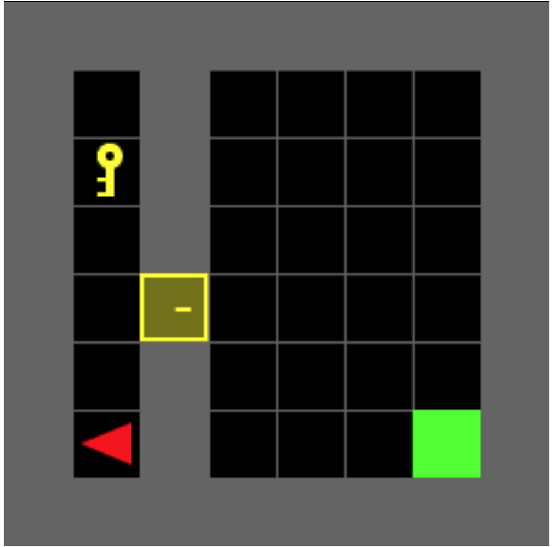
(a) MiniGrid Door Key

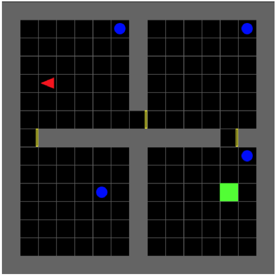
(b) 4 Rooms with Balls

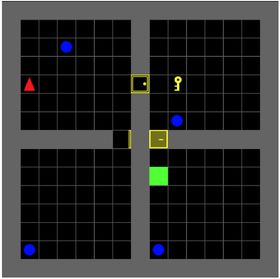
(c) 4 Rooms with a Locked Door

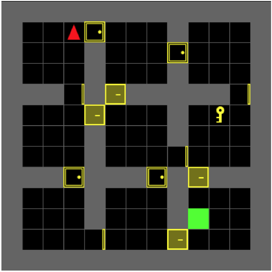
(d) 9 Rooms with Locked Doors

Figure 1: Example of MiniGrid-based instances: From left to right, we show one instance from each RL problem domain with additional task structures. A single planning task annotates each problem domain, and each domain randomizes the location of the objects.

Solving PaRL Task

In this section, we present HRL algorithms for solving PaRL tasks $E:=\langle{\mathcal{M}},\Pi,L\rangle$. For any pair of initial state $s_{0}\in\mathcal{S}$ and a goal $s_{g}\in G$ in ${\mathcal{M}}$, we can generate a sequence of options {${O}_{o_{1}},{O}_{o_{2}},\ldots,{O}_{o_{k}}$} from a plan in $\Pi$ that reaches the goal state $L(s_{g})\in\mathcal{S}^{\prime}$ from the initial state $L(s_{0})\in\mathcal{S}^{\prime}$. Therefore, we can invoke AI planners in two ways, either precompute those option-level plans offline or generate plans while training option policies online. In this paper, we focus on the online approach that integrates AI planner as a higher level control agent and model-free RL as lower-level agents in HRL architecture.

Algorithm 1 shows the outline of HRL agent that learns options online with a PaRL task. The algorithm alternates rollout and training phases until the limit on the number of iterations is reached. In the rollout phase, HRL agent selects an option ${O}_{o}$ using any AI planner by solving the annotating planning task $\Pi$ with the initial planning state $s^{\prime}_{0}$ being the current planning state $L(s)$ and returning the applicable planning operator in $s^{\prime}{0}$ (line 6). Note that this re-planning at every option selection step formulate the option selection as an action selection in online planning (Mausam and Kolobov 2012), it is much more efficient than learning-based approaches. If ${O}_{o}$ was not created before, we create the option and initialize the policy $\pi_{{O}_{o}}$ and add it to a container (lines 7-8). Next, sample trajectories are generated by using $\pi_{{O}_{o}}$ until it terminates, and for each one-step state transition, we compute the intrinsic reward following Definition 7 (lines 10-12). Then, HRL agent updates the option policy using the samples stored in the buffer in the training phase by any model-RL algorithm (line 15).

In our experiments, we integrated $A^{*}$ algorithm implemented in Pyperplan (Alkhazraji et al. 2016) with double DQN (DDQN) (Van Hasselt, Guez, and Silver 2016) and Proximal Policy Optimization PPO (Schulman et al. 2017) for option policy training, yielding two algorithms: HRL with integrated planning and PPO (HplanPPO) and HRL with integrated planning and DDQN HplanDDQN. Algorithm 2 shows HplanPPO, creating a separate PPO agent per option. Option training phases do not share samples (an on-policy method). HplanDDQN is similar to HplanPPO except for it only creates a single DDQN agent that augments the input to DDQN network with a one-hot encoding of option labels, allowing reuse of the samples for training option policies.

Experiments

All experiments are conducted in a cluster computing environment equipped with Intel (R) Xeon(R) Gold 6258R CPUs and NVIDIA A-100/V-100 GPUs. For each run, we limited computational resources to utilize up to 16 GB of memory with 2 CPUs and 1 GPU. For HRL experiments, we created two benchmark sets. The first benchmark set extends MiniGrid environment (Chevalier-Boisvert, Willems, and Pal 2018) with more complex task structures than the predefined environments inspired by BabyAI environment (Chevalier-Boisvert et al. 2019). During training RL/HRL algorithms, we reset the environments with the same random seeds from 0 to 999 and excluded existing baseline algorithms relying on tabular Q-learning.

The second benchmark set extends four rooms navigation domain on a larger scale with a maze-like topology. Namely, we extend to 4 rooms on a 20x20 grid and 12 rooms on a 16x16 grid only allowing a single path that connects all the rooms.

Algorithms

We evaluate HplanPPO and HplanDDQN algorithms and compare them with existing baseline algorithms from the flat RL counterparts, PPO and DDQN, and Deep Hierarchical Reward Machines (HRM) (Icarte et al. 2022). We implemented all algorithms by extending stable-baselines3 (Raffin et al. 2021), except for HRM, which offers open-source implementation by the original authors. In the experiments in MiniGrid environments, we evaluated each algorithm at least 5 times, and report the average, the minimum and maximum range, and 95 percent confidence intervals in the plots. Due to the space limit, we will provide details on general experiment setups and implementation of deep neural network architectures and hyper-parameter choices in the Appendix.

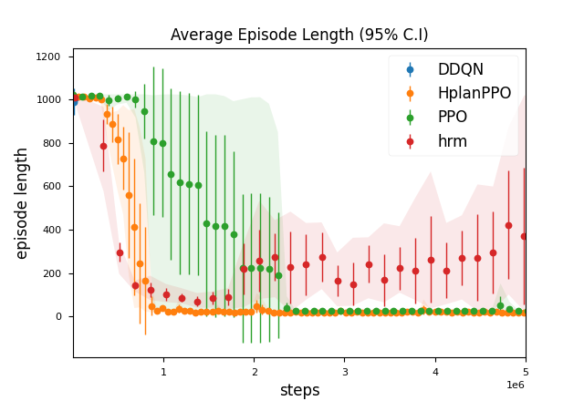
(a) DoorKey

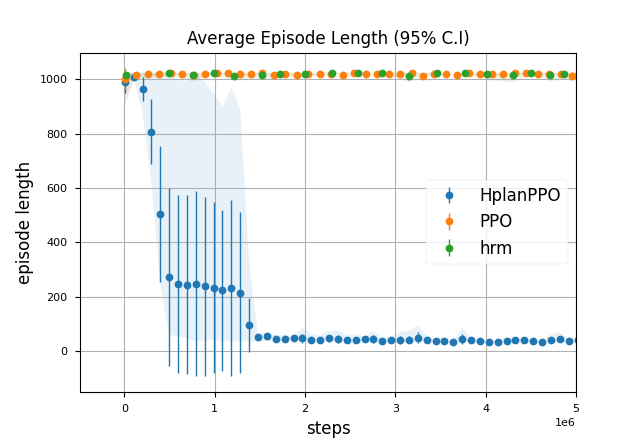
(b) 4 Rooms with Balls

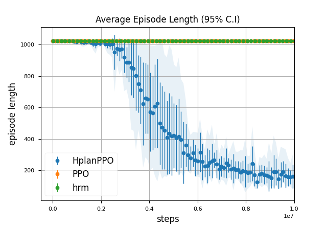
(c) 4 Rooms with a Locked Door

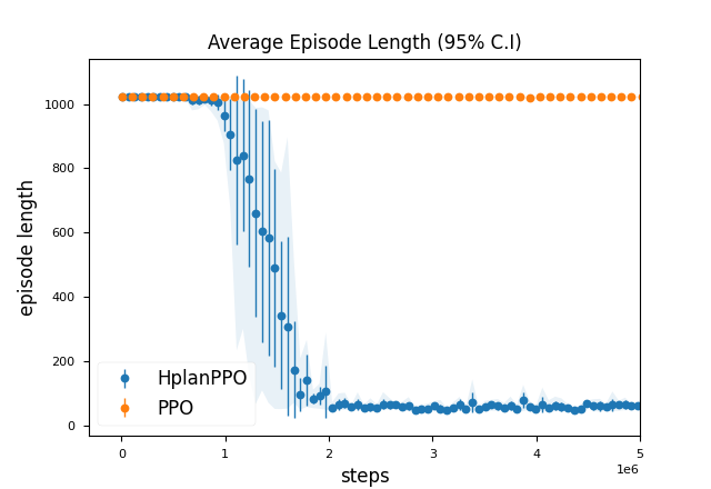
(d) 9 Rooms with Locked Doors

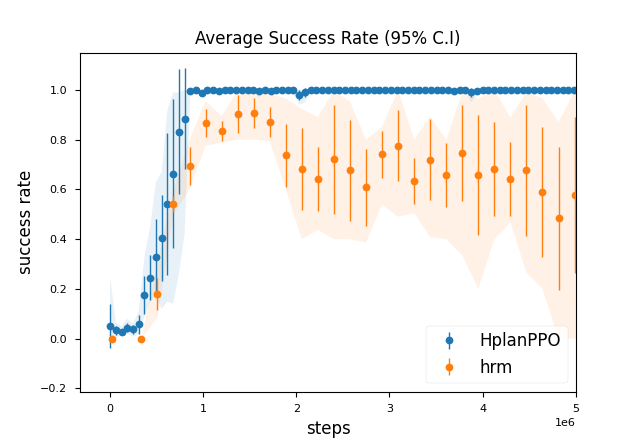
(e) DoorKey

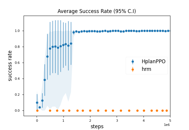
(f) 4 Rooms with Balls

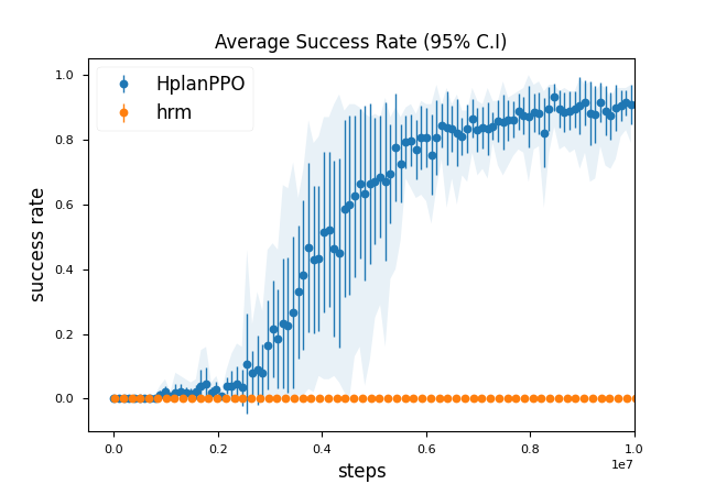
(g) 4 Rooms with a Locked Door

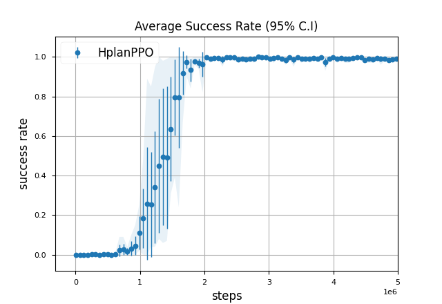
(h) 9 Rooms with Locked Doors

Figure 2: Average episode length (a)-(d) and average success rate (e)-(h) on MiniGrid-based instances.

MiniGrid-based Benchmark Problems

Figure 1 illustrates examples of four MiniGrid-based RL environments. Each RL environment can vary the location of objects such as a key, door, or the goal tile. In addition to such random variations, we introduced the following task structures that can be captured by a single planning annotation task per RL domain. MiniGrid Door Key in Figure 1(a), the high-level task of the agent is to pick up the key, unlock the door and move to the goal location. Four rooms with Balls and Four rooms with a locked door both share a similar structure except for the Four rooms with a locked door domain requires an agent to use the key to unlock the door. The last Nine rooms with locked doors increase the number of rooms. Note that the symbolic state space in the planning annotation task abstracts away several details in MDP. First, the agent doesn’t know the precise location in the grid, but it knows the room that the agent stays in. Second, balls are invisible to the planning task, and the door state is also partially known to the planning agent. Namely, the planning agent cannot detect whether the door is closed or not. In addition to these modifications, we also assume that the environment is fully-observable MDP.

Comparison against Baselines

Figure 2 shows the average episode length and the success rate for solving MiniGrid based problem domains. Figure 2(a) and 2(e) show the result from MiniGrid DoorKey. First, we can see that both HplanPPO and HRM indeed improved the sample efficiency compared with flat RL baselines such as PPO. Comparing HRM and HplanDDQN, we see that HplanDDQN does not show notable progress in learning. We also observed that flat DDQN showed similar trends. Lastly, Figure 2(a) shows that the performance of HplanPPO is more stable than HRM since HplanPPO does not need to train the high-level control policy, solving instead the planning annotation task using AI planner.

In the four rooms domain and nine rooms domain, all other baseline algorithms, including HRM did not show notable learning progress. HplanPPO was the only algorithm that showed consistent and stable learning performance. First, the dimension of observation rapidly increase in 4 rooms domain and 9 rooms domain, each generating three channels of 15x15 and 22x22 arrays. Second, the underlying MDP of MiniGrid environment only feedbacks the agent with a sparse reward, $(1-\frac{0.9}{l})$ with $l$ being the length of the episode. In HplanPPO, it utilizes a more informative reward signal due to the intrinsic rewards derived from the planning states and the shorter episode length per terminating options.

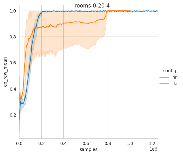
(a) Success rate on 20x20 grid

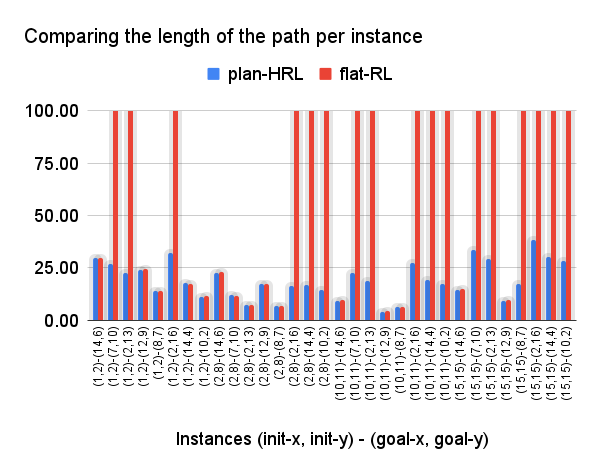
(b) Average episode length

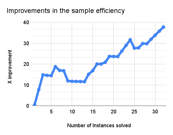
(c) Sample efficiency improvement rate

Figure 3: Success rate, average length, and improvement in sample efficiency on various size instances of rooms domain. (a) 4 rooms, 20x20 grid, (b)-(c) 12 rooms, 16x16 grid.

Rooms Domain

N-rooms domain modifies the classic 4-rooms domain by increasing the number of rooms and varying the size of the grids. In this problem, an agent moves on a grid, separated into N rooms, with narrow corridors connecting the adjacent rooms. The agent needs to move from a given location on the grid (in a given room) to a goal location (in a goal room).

In order to use the domain within our framework, we have created an abstract version of N-rooms planning domain and defined the state mapping function $L$ from the feature vectors in ${\mathcal{M}}$ encoding the coordinate on the grid to boolean vectors of the ground propositions in $\Pi_{M}$. As an example, in a four rooms domain on a N$\times$N grid, the PaRL task captures a total of 16 options that define all the movements between rooms and their adjacent corridors.

Figure 3(a) shows the learning curve from a 4 rooms domain on a 20x20 grid, comparing the success ratio for reaching the goal. In both PPO and HplanPPO, we gave a reward of +1 when reaching the goal, and a cost of -0.05 for each step. Comparing the results, we can see that the learning curves from HplanPPO (blue) reach a higher reward much earlier than PPO (orange).

Figure 3(b) compares the length of the path from an initial state to a goal state in a 16x16 grid 12 rooms domain. The x-axis shows different combinations of initial states and the goal state and the y-axis shows the number of steps to reaching the goal. In both PPO and HplanPPO cases, we allowed RL agents to reuse the policies trained in the previous problems. Figure 3(c) shows the improvement of the sample efficiency in HplanPPO when the options are reused over 32 different problem instances.

Related Work

Some of the relevant work that attempt to combine symbolic planning and RL include PEORL (Yang et al. 2018), SDRL (Lyu et al. 2019), and Taskable RL (Illanes et al. 2020). In Taskable RL, a manual mapping between the high-level actions in the planning task and the options in the RL task must be provided, and such a mapping could be many to one. The termination set also requires manual modifications. This makes it difficult to apply the method to a new RL task or even a different problem instance in the same problem domain. While PEORL also considers integrating symbolic planning and RL, it assumes that an exact representation of MDP is available in the planning task and that there is one option per planning transition, which is unrealistic in many domains. It updates the value function and the associated option policies only when options terminate, while our method can operate online to accommodate intra-option updates. Moreover, PEORL is based on tabular representation, while our method is based on deep neural network representation. SDRL, the deep learning extension of PEORL, still learns both the lower-level and the high-level policies in restricted setting, whereas our method can use any RL algorithm for option policy learning. A complementary to our work is the work is model learning (Jin et al. 2022), discovering the planning model that we assume to be given.

Recently, there has been a series of work on using reward machines and linear temporal logic (LTL) for defining finite state automata encapsulating high-level symbolic information. The information is used to define either reward (Camacho et al. 2019; Icarte et al. 2022) or options (Icarte et al. 2018). The main difference of these methods from ours is that these methods encode abstract or partial solutions, and thus require someone to first solve the problem, at least on an abstract level. These solutions need to be updated once moving to solving even somewhat similar tasks. Further, while LTLs allow for capturing complex logical expressions, only a very restricted fragment is within reach of RL algorithms, even theoretically (Yang, Littman, and Carbin 2022).

Conclusions and Future Work

In this work, we have presented a simple general framework for annotating reinforcement learning tasks with planning tasks, to facilitate the transfer of planning based techniques into the field of reinforcement learning. Our framework links the state abstraction in AI planning and temporal abstraction in RL, providing a way to decompose the MDP into sub-MDPs by specifying options initiation set and termination condition based on planning operator definitions. We design a general method for injecting intrinsic rewards to RL agents from the abstract planning task by reformulating the underlying decomposed sub-MDPs with constraints visible to planning agents. Learning only the (intra-option) policies for these sub-MDPs is shown to work well in practice on various problems, significantly improving sample efficiency.

This, however, is not the end of the road. While this work focused on temporal abstractions, our framework is more general, allowing to inject knowledge from the annotated planning task into the MDP. One example of such knowledge is goal distance estimates that can be used for reward shaping (Gehring et al. 2021). Another example is landmarks (Porteous, Sebastia, and Hoffmann 2001) (logical formula that must occur on all plans), that can be used as sub-goals. Planning research has been focusing for years on automatically extracting knowledge from the planning task description. We believe that injecting this knowledge into the MDP can greatly improve the performance of RL agents.

Appendix A Planning Annotations

This section summarizes the planning annotations for MiniGrid and N Rooms domains that we evaluated in the experiment section.

A.1 MiniGrid

The RL environment maintains rooms over an NxN grid, blue balls, a green goal tile, the agent location and orientation, and doors with states, open, closed, locked, and unlocked. In planning tasks, we abstract away information relevant to each cell in the grid. Namely, the exact location and orientation of the agent, the exact location of the key, blue balls, and a green goal tile are all ignored. In addition, the states of a door is simplified to two states, locked or unlocked.

On resetting the RL environment, we implemented gym environments such that objects that are only visible to RL environments are randomized, as usual in the standard MiniGrid gym environment. However, we restricted the information relevant to the planning task remains the same. For example, the agent’s initial location will be randomized within a predefined room (the room at the upper left corner), and the goal location will also be randomized within a room at the lower right corner. A key will appear in the same room, and the initial state of the door, whether it is locked or unlocked, will remain the same. This choice doesn’t limit algorithms but it simplifies the experiment to start with a single PDDL instance to annotate the environment, although the agent will generate additional PDDL instances when it solves planning tasks with a new initial planning state while selecting options online.

PDDL domain

PDDL domain file was manually generated by modifying existing similar PDDL domains.

(define (domain MazeRooms)
  (:requirements :strips :typing)
    (:types
        room - object
        key - object
        door - object
    )
    (:predicates
        (at-agent ?r - room)                        ; Agent current location
        (at ?k - key ?r - room)                     ; Key location
        (carry ?k - key)                            ; Does agent carry the key
        (empty-hand)                                ; Is agent hand empty
        (unlocked ?d - door)                        ; Is door unlocked
        (locked ?d - door)                          ; Is door locked (for STRIPS only)
        (KEYMATCH ?k - key ?d - door)               ; Does the key match the door
        (LINK ?d - door ?r1 - room ?r2 - room)      ; Two rooms linked via the door
    )

    (:action move-room
        :parameters (?d - door ?r1 - room ?r2 - room)
        :precondition (and
            (LINK ?d ?r1 ?r2)
            (at-agent ?r1)
            (unlocked ?d)
        )
        :effect (and
            (not (at-agent ?r1))
            (at-agent ?r2)
        )
    )

    (:action pickup
        :parameters (?k - key ?r - room)
        :precondition (and
            (at ?k ?r)
            (at-agent ?r)
            (empty-hand)
        )
        :effect (and
            (not (at ?k ?r))
            (not (empty-hand))
            (carry ?k)
        )
    )

    (:action drop
        :parameters (?k - key ?r - room)
        :precondition (and
            (carry ?k)
            (at-agent ?r)
        )
        :effect (and
            (at ?k ?r)
            (empty-hand)
            (not (carry ?k))
        )
    )

    (:action unlock
        :parameters (?k - key ?d - door ?r1 - room ?r2 - room)
        :precondition (and
            (LINK ?d ?r1 ?r2)
            (KEYMATCH ?k ?d)
            (at-agent ?r1)
            (carry ?k)
            (locked ?d)
        )
        :effect (and
            (not (locked ?d))
            (unlocked ?d)
        )
    )

    (:action lock
        :parameters (?k - key ?d - door ?r1 - room ?r2 - room)
        :precondition (and
            (LINK ?d ?r1 ?r2)
            (KEYMATCH ?k ?d)
            (at-agent ?r1)
            (carry ?k)
            (unlocked ?d)
        )
        :effect (and
            (locked ?d)
            (not (unlocked ?d))
        )
    )
)

PDDL instance

All PDDL problem instances were generated by our benchmark script code by processing internal state information available in MiniGrid gym environments.

Figure 4: DoorKey

(define (problem MazeRooms-8by8-DoorKey)
    (:domain MazeRooms)
    (:objects
        R-0-0 R-1-0 -  room
        K-yellow-0 - key
        D-yellow-0-0-1-0 - door
    )
    (:init
        (LINK D-yellow-0-0-1-0 R-0-0 R-1-0)
        (LINK D-yellow-0-0-1-0 R-1-0 R-0-0)
        (KEYMATCH K-yellow-0 D-yellow-0-0-1-0)
        (at-agent R-0-0)
        (at K-yellow-0 R-0-0)
        (locked D-yellow-0-0-1-0)
        (empty-hand)
    )
    (:goal (and
        (at-agent R-1-0))
    )
)

Figure 5: 4 Rooms with Balls

(define (problem MazeRooms-2by2-Balls)
    (:domain MazeRooms)
    (:objects
        R-0-0 R-0-1 R-1-0 R-1-1 -  room
        D-yellow-0-0-1-0 D-yellow-1-0-1-1 D-yellow-0-0-0-1 - door
    )
    (:init
        (LINK D-yellow-0-0-0-1 R-0-0 R-0-1)
        (LINK D-yellow-0-0-0-1 R-0-1 R-0-0)
        (LINK D-yellow-0-0-1-0 R-0-0 R-1-0)
        (LINK D-yellow-0-0-1-0 R-1-0 R-0-0)
        (LINK D-yellow-1-0-1-1 R-1-0 R-1-1)
        (LINK D-yellow-1-0-1-1 R-1-1 R-1-0)
        (at-agent R-0-0)
        (unlocked D-yellow-0-0-0-1)
        (unlocked D-yellow-0-0-1-0)
        (unlocked D-yellow-1-0-1-1)
        (empty-hand)
    )
    (:goal (and
        (at-agent R-1-1))
    )
)

Figure 6: 4 Rooms with a Locked Door

(define (problem MazeRooms-2by2-Locked)
    (:domain MazeRooms)
    (:objects
        R-0-0 R-0-1 R-1-0 R-1-1 -  room
        K-yellow-0 - key
        D-yellow-0-0-1-0 D-yellow-1-0-1-1 D-yellow-0-0-0-1 - door
    )
    (:init
        (LINK D-yellow-0-0-0-1 R-0-0 R-0-1)
        (LINK D-yellow-0-0-0-1 R-0-1 R-0-0)
        (LINK D-yellow-0-0-1-0 R-0-0 R-1-0)
        (LINK D-yellow-0-0-1-0 R-1-0 R-0-0)
        (LINK D-yellow-1-0-1-1 R-1-0 R-1-1)
        (LINK D-yellow-1-0-1-1 R-1-1 R-1-0)
        (KEYMATCH K-yellow-0 D-yellow-0-0-0-1)
        (KEYMATCH K-yellow-0 D-yellow-0-0-1-0)
        (KEYMATCH K-yellow-0 D-yellow-1-0-1-1)
        (at-agent R-0-0)
        (at K-yellow-0 R-1-0)
        (locked D-yellow-1-0-1-1)
        (unlocked D-yellow-0-0-0-1)
        (unlocked D-yellow-0-0-1-0)
        (empty-hand)
    )
    (:goal (and
        (at-agent R-1-1))
    )
)

Figure 7: 9 Rooms with Locked Doors

(define (problem MazeRooms-3by3-LockedDoors)
    (:domain MazeRooms)
    (:objects
        R-0-0 R-0-1 R-0-2 R-1-0 R-1-1 R-1-2 R-2-0 R-2-1 R-2-2 -  room
        K-yellow-0 - key
        D-yellow-0-1-0-2 D-yellow-1-1-2-1 D-yellow-2-0-2-1
        D-yellow-2-1-2-2 D-yellow-0-2-1-2 D-yellow-1-0-2-0
        D-yellow-1-1-1-2 D-yellow-0-0-1-0 D-yellow-0-0-0-1
        D-yellow-1-0-1-1 D-yellow-0-1-1-1 D-yellow-1-2-2-2 - door
    )
    (:init
        (LINK D-yellow-0-0-0-1 R-0-0 R-0-1)
        (LINK D-yellow-0-0-0-1 R-0-1 R-0-0)
        (LINK D-yellow-0-0-1-0 R-0-0 R-1-0)
        (LINK D-yellow-0-0-1-0 R-1-0 R-0-0)
        (LINK D-yellow-0-1-0-2 R-0-1 R-0-2)
        (LINK D-yellow-0-1-0-2 R-0-2 R-0-1)
        (LINK D-yellow-0-1-1-1 R-0-1 R-1-1)
        (LINK D-yellow-0-1-1-1 R-1-1 R-0-1)
        (LINK D-yellow-0-2-1-2 R-0-2 R-1-2)
        (LINK D-yellow-0-2-1-2 R-1-2 R-0-2)
        (LINK D-yellow-1-0-1-1 R-1-0 R-1-1)
        (LINK D-yellow-1-0-1-1 R-1-1 R-1-0)
        (LINK D-yellow-1-0-2-0 R-1-0 R-2-0)
        (LINK D-yellow-1-0-2-0 R-2-0 R-1-0)
        (LINK D-yellow-1-1-1-2 R-1-1 R-1-2)
        (LINK D-yellow-1-1-1-2 R-1-2 R-1-1)
        (LINK D-yellow-1-1-2-1 R-1-1 R-2-1)
        (LINK D-yellow-1-1-2-1 R-2-1 R-1-1)
        (LINK D-yellow-1-2-2-2 R-1-2 R-2-2)
        (LINK D-yellow-1-2-2-2 R-2-2 R-1-2)
        (LINK D-yellow-2-0-2-1 R-2-0 R-2-1)
        (LINK D-yellow-2-0-2-1 R-2-1 R-2-0)
        (LINK D-yellow-2-1-2-2 R-2-1 R-2-2)
        (LINK D-yellow-2-1-2-2 R-2-2 R-2-1)
        (KEYMATCH K-yellow-0 D-yellow-0-0-0-1)
        (KEYMATCH K-yellow-0 D-yellow-0-0-1-0)
        (KEYMATCH K-yellow-0 D-yellow-0-1-0-2)
        (KEYMATCH K-yellow-0 D-yellow-0-1-1-1)
        (KEYMATCH K-yellow-0 D-yellow-0-2-1-2)
        (KEYMATCH K-yellow-0 D-yellow-1-0-1-1)
        (KEYMATCH K-yellow-0 D-yellow-1-0-2-0)
        (KEYMATCH K-yellow-0 D-yellow-1-1-1-2)
        (KEYMATCH K-yellow-0 D-yellow-1-1-2-1)
        (KEYMATCH K-yellow-0 D-yellow-1-2-2-2)
        (KEYMATCH K-yellow-0 D-yellow-2-0-2-1)
        (KEYMATCH K-yellow-0 D-yellow-2-1-2-2)
        (at-agent R-0-0)
        (at K-yellow-0 R-2-1)
        (locked D-yellow-0-1-1-1)
        (locked D-yellow-1-0-1-1)
        (locked D-yellow-1-2-2-2)
        (locked D-yellow-2-1-2-2)
        (unlocked D-yellow-0-0-0-1)
        (unlocked D-yellow-0-0-1-0)
        (unlocked D-yellow-0-1-0-2)
        (unlocked D-yellow-0-2-1-2)
        (unlocked D-yellow-1-0-2-0)
        (unlocked D-yellow-1-1-1-2)
        (unlocked D-yellow-1-1-2-1)
        (unlocked D-yellow-2-0-2-1)
        (empty-hand)
    )
    (:goal (and
        (at-agent R-2-2))
    )
)

A.2 N-rooms

The RL environment maintains an NxN grid with the location of rooms, hallways, and walls. Therefore, a planning state obtained from an RL state through the state mapping function is the name of each room associated with the location.

PDDL domain

The PDDL domain file used for the N-rooms problem is described in what follows.

(define (domain rooms)
  (:requirements :strips :typing)
    (:types
        room - object
    )
    (:predicates Ψ
        (in-room ?r - room)                         ; Agent current location
        (CONNECTED-ROOMS ?r - room ?s - room)       ; Two rooms are connected
    )
    (:action move-room
        :parameters (?r - room ?s - room)
        :precondition (and
            (CONNECTED-ROOMS ?r ?s)
            (in-room ?r)
        )
        :effect (and
            (not (in-room ?r))
            (in-room ?s)
        )
    )
)

PDDL instance

Unlike MiniGrid-based environments, we randomize both initial and goal locations on resetting the gym environment. Therefore, we show one of the auto-generated planning instances associated with a pair of initial and goal rooms.

(define (problem rooms-1-16-12__1-2)
    (:domain rooms)
    (:objects
        W c-r0-r2 c-r10-r3 c-r11-r5 c-r2-r1 c-r2-r9 c-r3-r7
        c-r4-r8 c-r4-r9 c-r6-r3 c-r8-r5 c-r9-r10
        r0 r1 r10 r11 r2 r3 r4 r5 r6 r7 r8 r9 - room
    )
    (:init
        (CONNECTED-ROOMS c-r0-r2 r0)
        (CONNECTED-ROOMS c-r0-r2 r2)
        (CONNECTED-ROOMS c-r10-r3 r10)
        (CONNECTED-ROOMS c-r10-r3 r3)
        (CONNECTED-ROOMS c-r11-r5 r11)
        (CONNECTED-ROOMS c-r11-r5 r5)
        (CONNECTED-ROOMS c-r2-r1 r1)
        (CONNECTED-ROOMS c-r2-r1 r2)
        (CONNECTED-ROOMS c-r2-r9 r2)
        (CONNECTED-ROOMS c-r2-r9 r9)
        (CONNECTED-ROOMS c-r3-r7 r3)
        (CONNECTED-ROOMS c-r3-r7 r7)
        (CONNECTED-ROOMS c-r4-r8 r4)
        (CONNECTED-ROOMS c-r4-r8 r8)
        (CONNECTED-ROOMS c-r4-r9 r4)
        (CONNECTED-ROOMS c-r4-r9 r9)
        (CONNECTED-ROOMS c-r6-r3 r3)
        (CONNECTED-ROOMS c-r6-r3 r6)
        (CONNECTED-ROOMS c-r8-r5 r5)
        (CONNECTED-ROOMS c-r8-r5 r8)
        (CONNECTED-ROOMS c-r9-r10 r10)
        (CONNECTED-ROOMS c-r9-r10 r9)
        (CONNECTED-ROOMS r0 c-r0-r2)
        (CONNECTED-ROOMS r1 c-r2-r1)
        (CONNECTED-ROOMS r10 c-r10-r3)
        (CONNECTED-ROOMS r10 c-r9-r10)
        (CONNECTED-ROOMS r11 c-r11-r5)
        (CONNECTED-ROOMS r2 c-r0-r2)
        (CONNECTED-ROOMS r2 c-r2-r1)
        (CONNECTED-ROOMS r2 c-r2-r9)
        (CONNECTED-ROOMS r3 c-r10-r3)
        (CONNECTED-ROOMS r3 c-r3-r7)
        (CONNECTED-ROOMS r3 c-r6-r3)
        (CONNECTED-ROOMS r4 c-r4-r8)
        (CONNECTED-ROOMS r4 c-r4-r9)
        (CONNECTED-ROOMS r5 c-r11-r5)
        (CONNECTED-ROOMS r5 c-r8-r5)
        (CONNECTED-ROOMS r6 c-r6-r3)
        (CONNECTED-ROOMS r7 c-r3-r7)
        (CONNECTED-ROOMS r8 c-r4-r8)
        (CONNECTED-ROOMS r8 c-r8-r5)
        (CONNECTED-ROOMS r9 c-r2-r9)
        (CONNECTED-ROOMS r9 c-r4-r9)
        (CONNECTED-ROOMS r9 c-r9-r10)
        (in-room r6)
    )
    (:goal (and
        (in-room r0))
    )
)

Appendix B Hierarchical Reward Machines

Hierarchical Reward Machine (HRM) needs a Finite State Machine (FSM) that describes the transitions between symbolic states and events that trigger the transitions. It can either be written directly or translated from Linear Temporal Logic (LTL) expressions. In this paper, we defined FSMs for MiniGrid environments following the structures that commonly appear in papers based on reward machines.

Note that FSMs in HRL algorithms based on LTL/RM encodes knowledge about the solution to the problem. FSMs must be defined per instance basis, or a human expert must know a partial solution that is general enough so that it can be applied to multiple instances. As the problem domain gets more complicated, this manual task is not at all trivial.

In this paper, we chose hierarchical reward machines (HRM) (Icarte et al. 2022) as a baseline HRL algorithm since it is very difficult to find a reliable implementation that integrates deep RL agents. While extending the baseline for solving MiniGrid environments, we defined FSMs similar to the ones in the baseline method (Icarte et al. 2022).

B.1 MiniGrid - DoorKey

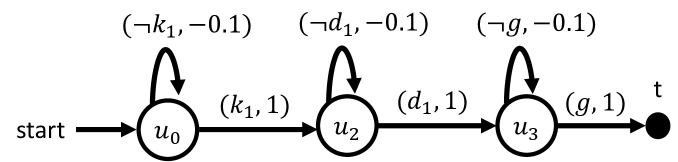
Figure 8: DoorKey

Nodes $u_{0}$, $u_{1}$, and $u_{2}$ are FSM states. Upon resetting the RL environment, FSM enters the first node $u_{0}$, and events defined over the edges trigger the state transitions. This reward structure can be used for defining rewards for the RL environment in a reward machine, or one could define options over FSMs that encapsulates temporarily extended actions. The events are defined as follows: $k_{1}$ entails true if the agent picked up the key at the room, $d_{1}$ entails true if the agent was able to unlock the door connecting two rooms, $g$ entails true if the agent arrived at the goal room. Finally, the FSM terminates when the agent arrives at the goal tile. The value next to the event is the reward that the agent receives. For example, when the agent was in state $u_{0}$ and did not pick up the key, then the reward is $-0.1$. On the other hand, if the agent picked up the key, then the state transition occurs, and the agent receives a reward of $1$.

B.2 MiniGrid - 4 Rooms with Balls

Figure 9: 4 Rooms with Balls

The underlying idea for defining this FSM is the same for the FSM shown in Figure 8. In this problem domain, there are 3 doors that connect rooms. $d_{1}$ entails true if the agent unlocked the room between the upper left and the upper right rooms, $d_{1}$ entails true if the agent unlocked the room between the upper right and the lower right rooms.

B.3 MiniGrid - 4 Rooms with a Locked Door

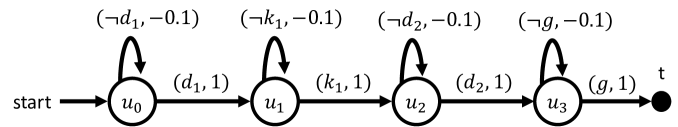
Figure 10: 4 Rooms with a Locked Door

In this problem domain, the agent musts use a key to unlocked the goal room. Therefore, Figure 10 encodes such knowledge in the FSM; from state $u_{1}$, the agent can transit to the next state if agent picked up the key in the room at the upper right corner ($k_{1}$). As we can see, as the solution to the problem becomes more complex, the FSMs has to incorporate such knowledge in more complex diagrams, one per each domain. It is worth noting that in order to incorporate the knowledge about solutions in the FSM, one needs first to obtain such knowledge. While for small problems humans can easily spot what a solution is, as problems become more complex, it becomes harder.

Appendix C Implementation Notes

In this section, we provide implementation details for HplanPPO, HplanDDQN, and HRM. For more additional details, please refer to the python script code available in the code supplementary material.

C.1 Feature Extractors

For the problem domains generated by MiniGrid environment, we modified Convolutional Neural Network (CNN) based architecture presented in BabyAI RL environment (Chevalier-Boisvert et al. 2019). The main differences between BabyAI and our MiniGrid-based gym environments are: (1) our experiments are fully-observable, (2) there’s no natural language goal description available in our experiments.

CNN Feature Extractors for 4 and 9 Rooms Environments

The CNN feature extractors first process three-channel input grid into the embedding layer since the value at each grid encodes symbolic state information in integers. Next, we pass 3-layer CNN, and finally we added the last linear layer to the output the feature vector of size 128.

class BabyAIFullyObsCNN(BaseFeaturesExtractor):
    def __init__(
        self,
        observation_space: gym.Space,
        features_dim: int = 128,
    ):
        super().__init__(observation_space, features_dim)
        self.max_value = 147
        self.embedding = nn.Embedding(3 * self.max_value, features_dim)
        self.cnn = nn.Sequential(
            nn.Conv2d(in_channels=features_dim, out_channels=features_dim,
            kernel_size=(3, 3), stride=(2, 2), padding=1),
            nn.BatchNorm2d(features_dim),
            nn.ReLU(),
            nn.Conv2d(in_channels=features_dim, out_channels=features_dim,
            kernel_size=(3, 3), stride=(2, 2), padding=1),
            nn.BatchNorm2d(features_dim),
            nn.ReLU(),
            nn.Conv2d(in_channels=features_dim, out_channels=features_dim,
            kernel_size=(3, 3), stride=(2, 2), padding=1),
            nn.BatchNorm2d(features_dim),
            nn.ReLU(),
            nn.MaxPool2d(kernel_size=(2, 2), stride=(2, 2), padding=0),
            nn.Flatten()
        )
        self.linear = nn.Sequential(
            nn.Linear(n_flatten, features_dim),
            nn.ReLU()
        )
        self.apply(initialize_parameters)

    def forward(self, observations: th.Tensor):
        offsets = th.Tensor([0, self.max_value, 2 * self.max_value])
        x = (observations + offsets[None, :, None, None]).long()
        x =  self.embedding(x).sum(1).permute(0, 3, 1, 2)
        x = self.cnn(x)
        x = self.linear(x)
        return x

CNN Feature Extractors for Door Key environment

The architecture remains the same as above except for the CNN only has two layers when the input dimension becomes smaller. In addition to processing the feature values in the grid, the following code snippet also shows the option labels will also be concatenated with the feature vector after passing an embedding layer and one additional linear layer. These option label features are necessary for implementing DDQN-based algorithms.

class BabyAIFullyObsSmallCNNDict(BaseFeaturesExtractor):
    def __init__(
            self,
            observation_space: gym.Space,
            features_dim: int = 128,
    ):
        super().__init__(observation_space, features_dim)
        image_observation_space = observation_space.spaces[’image’]

        self.max_value = 147
        self.embedding = nn.Embedding(3 * self.max_value, features_dim)
        self.cnn = nn.Sequential(
            nn.Conv2d(in_channels=features_dim, out_channels=features_dim,
            kernel_size=(3, 3), stride=(2, 2), padding=1),
            nn.BatchNorm2d(features_dim),
            nn.ReLU(),
            nn.Conv2d(in_channels=features_dim, out_channels=features_dim,
            kernel_size=(3, 3), stride=(2, 2), padding=1),
            nn.BatchNorm2d(features_dim),
            nn.ReLU(),
            nn.MaxPool2d(kernel_size=(2, 2), stride=(2, 2), padding=0),
            nn.Flatten()
        )
        self.linear = nn.Sequential(
            nn.Linear(n_flatten, features_dim),
            nn.ReLU()
        )
        label_observation_space = observation_space.spaces[’label’]
        self.label_embedding = nn.Linear(label_observation_space.n, features_dim)
        self.linear2 = nn.Sequential(
            nn.Linear(features_dim * 2, features_dim),
            nn.ReLU()
        )
        self.apply(initialize_parameters)  # Initialize parameters correctly

    def forward(self, observations: th.Tensor) -> th.Tensor:
        x = observations[’image’]
        offsets = th.Tensor([0, self.max_value, 2 * self.max_value]).to(x.device)
        x = (x + offsets[None, :, None, None]).long()
        x = self.embedding(x).sum(1).permute(0, 3, 1, 2)
        x = self.cnn(x)
        x = self.linear(x)
        y = observations[’label’]
        y = th.squeeze(y)
        y = self.label_embedding(y)
        if y.ndim == 1:
            y = y.reshape((1, -1))
        z = th.cat((x,y), dim=1)
        z = self.linear2(z)
        return z

Flattening Observation

Lastly, we also tested a features extractor that flattens the input observations in 2-D arrays into a single 1-D array with one-hot encoding. This flattening observation feature extractors are used in N-rooms environments and the original code implementation in hierarchical reward machines (Icarte et al. 2022).

C.2 PPO Hyperparameters

MiniGrid-based Environments

• learning rate: $2.5e^{-4}$

• clip: 0.2

• option networks for policy and value: $[64,64]$

• flat RL networks for policy and value: $[128,128]$

• number of steps per rollout: 2048

• batch size: 256

• number of epochs for PPO update: 10

• gamma: 0.99

• lambda for GAE: 0.95

• entropy coefficient: 0.01

• value function coefficient: 0.5

• maximum gradient norm: 0.05

• maximum episode length: 1024

• option termination reward: +1

• option unit penalty cost: $\frac{0.9}{1024}$

N-rooms-based Environments

• learning rate: $1e^{-4}$

• clip: 0.1

• networks for policy and value: $[256,256]$

• number of steps per rollout: 2048

• batch size: 128

• number of epochs for PPO update: 10

• gamma: 0.99

• lambda for GAE: 0.95

• entropy coefficient: 0.01

• value function coefficient: 0.5

• maximum gradient norm: 0.05

• maximum episode length: 1024

• option termination reward: +1

• option unit penalty cost: -0.05

C.3 DDQN Hyperparameters

MiniGrid-based Environments

• replay buffer size: 149504

• learning rate: 0.0005

• learning starts: 1000

• batch size: 96

• tau: 1.0

• gamma: 0.9

• train frequency: 1 step

• gradient steps: 1

• target update interval: 500

• exploration fraction: 0.1

• exploration initial epsilon: 1.0

• exploration final epsilon: 0.1,

• max gradient norm: 10

• option networks for value: $[64,64]$

• flat RL networks for value: $[128,128]$

The DDQN hyperparameters are chosen from the baseline agent implementation (Icarte et al. 2022),

Appendix D More Results

D.1 MiniGrid DoorKey

Figure 11 shows learning progress of options and we show a shortest plan from annotated planning task.

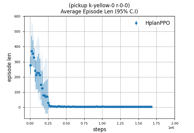
(a) (pickup k-yellow-0 r-0-0) Episode Length

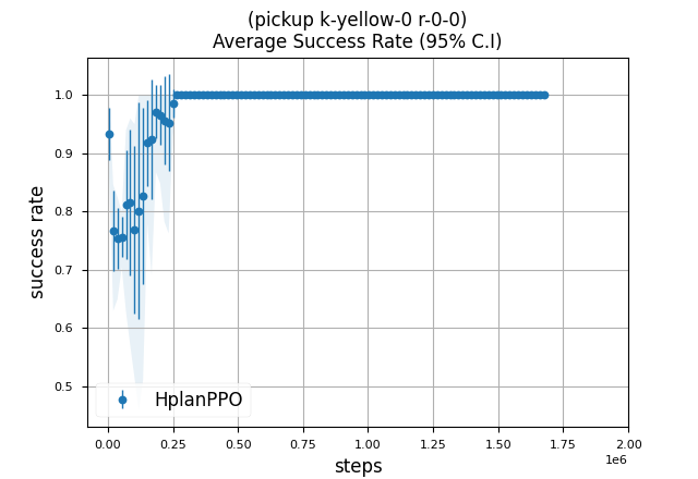
(b) (pickup k-yellow-0 r-0-0) Success Rate

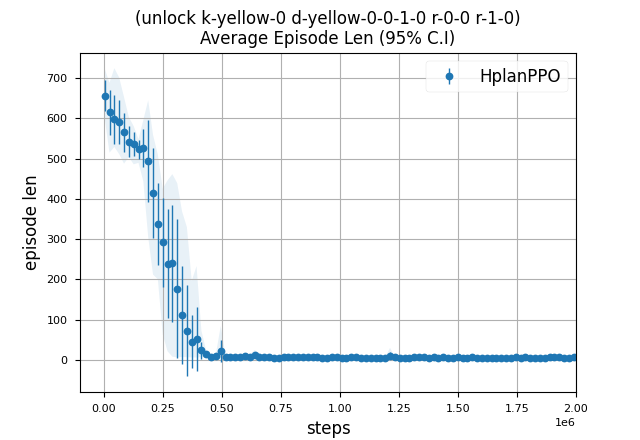
(c) unlock k-yellow-0 d-yellow-0-0-1-0 r-0-0 r-1-0) Episode Length

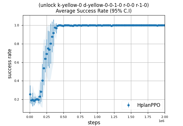
(d) unlock k-yellow-0 d-yellow-0-0-1-0 r-0-0 r-1-0) Success Rate

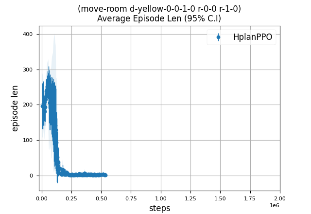
(e) (move-room d-yellow-0-0-1-0 r-0-0 r-1-0) Episode Length

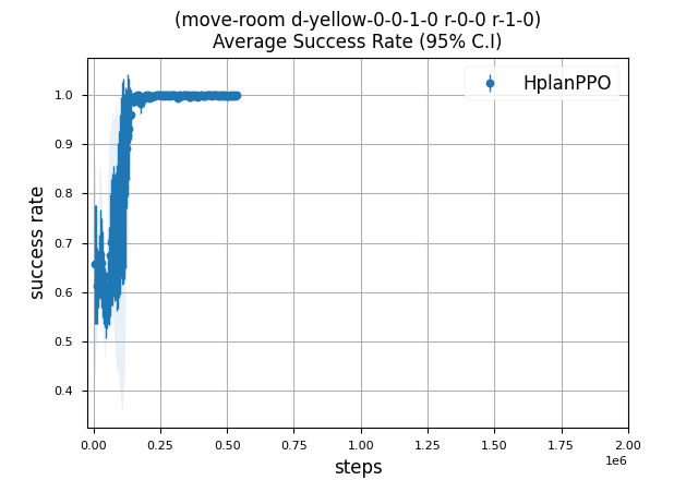
(f) (move-room d-yellow-0-0-1-0 r-0-0 r-1-0) Success Rate

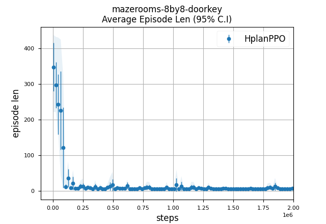
(g) Goal option Episode Length

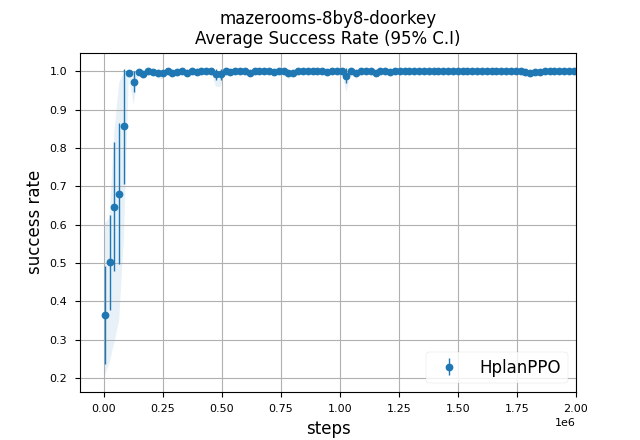
(h) Goal option Success Rate

Figure 11: Option Learning Progress in MiniGrid Door Key Domain

Plan from Annotated Planning Task

state:0
(locked d-yellow-0-0-1-0)
(at-agent r-0-0)
(empty-hand)
(at k-yellow-0 r-0-0)

action:0
(pickup k-yellow-0 r-0-0)
  PRE: (at k-yellow-0 r-0-0)
  PRE: (empty-hand)
  PRE: (at-agent r-0-0)
  ADD: (carry k-yellow-0)
  DEL: (at k-yellow-0 r-0-0)
  DEL: (empty-hand)

state:1
(carry k-yellow-0)
(locked d-yellow-0-0-1-0)
(at-agent r-0-0)

action:1
(unlock k-yellow-0 d-yellow-0-0-1-0 r-0-0 r-1-0)
  PRE: (carry k-yellow-0)
  PRE: (locked d-yellow-0-0-1-0)
  PRE: (at-agent r-0-0)
  ADD: (unlocked d-yellow-0-0-1-0)
  DEL: (locked d-yellow-0-0-1-0)

state:2
(carry k-yellow-0)
(unlocked d-yellow-0-0-1-0)
(at-agent r-0-0)

action:2
(move-room d-yellow-0-0-1-0 r-0-0 r-1-0)
  PRE: (unlocked d-yellow-0-0-1-0)
  PRE: (at-agent r-0-0)
  ADD: (at-agent r-1-0)
  DEL: (at-agent r-0-0)

D.2 MiniGrid 4 Rooms with a Locked Door

Figures 12 – 13 show learning progress of options and we show a shortest plan from annotated planning task.

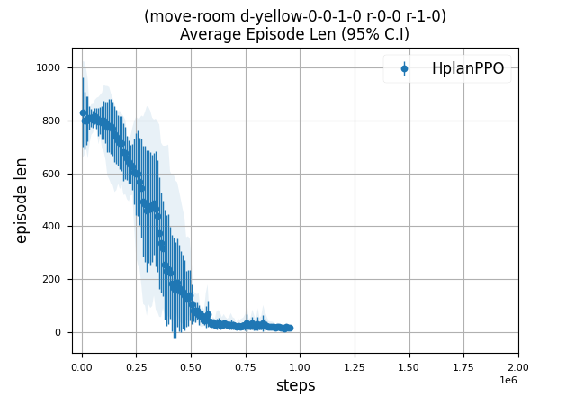
(a) (move-room d-yellow-0-0-1-0 r-0-0 r-1-0) Episode Length

(b) (move-room d-yellow-0-0-1-0 r-0-0 r-1-0) Success Rate

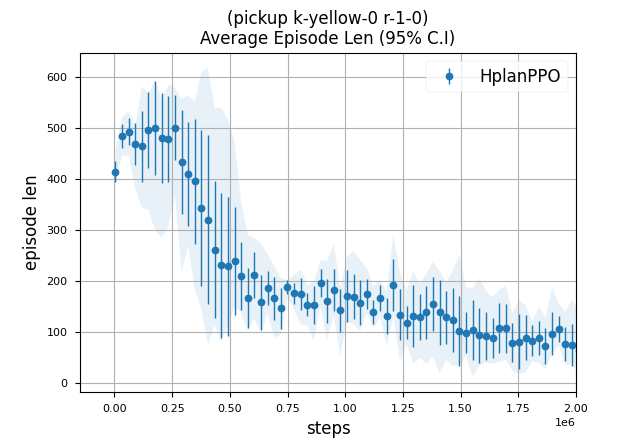
(c) (pickup k-yellow-0 r-1-0) Episode Length

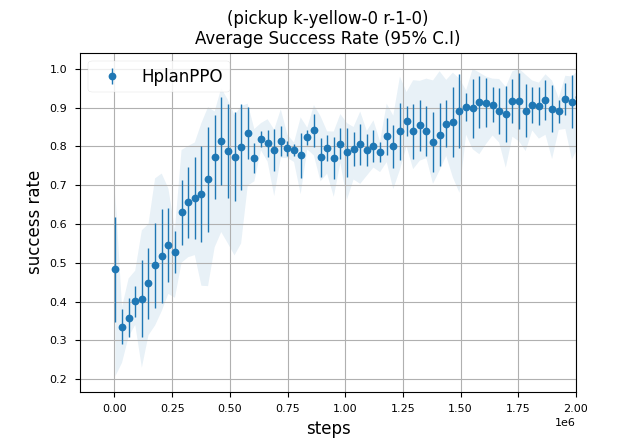
(d) (pickup k-yellow-0 r-1-0) Success Rate

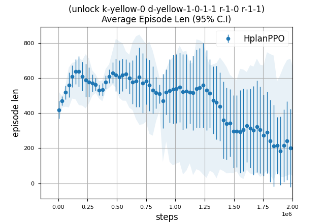
(e) (unlock k-yellow-0 d-yellow-1-0-1-1 r-1-0 r-1-1) Episode Length

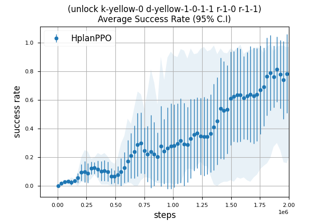
(f) (unlock k-yellow-0 d-yellow-1-0-1-1 r-1-0 r-1-1) Success Rate

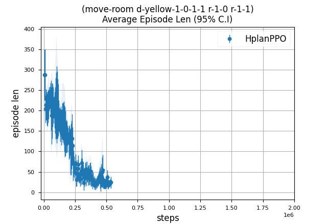
(g) (move-room d-yellow-1-0-1-1 r-1-0 r-1-1) Episode Length

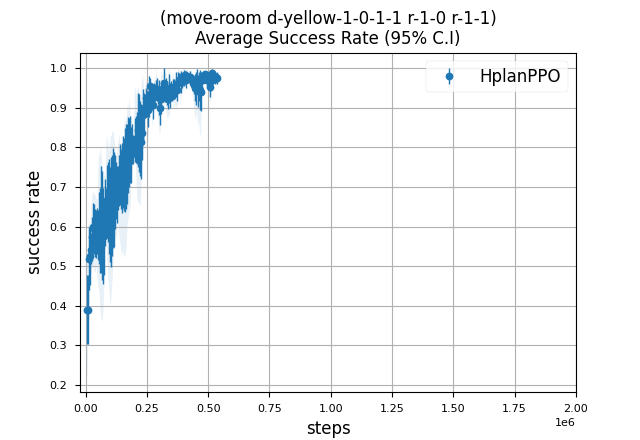
(h) (move-room d-yellow-1-0-1-1 r-1-0 r-1-1) Success Rate

Figure 12: Option Learning Progress in MiniGrid 4 Rooms with a Locked Door Domain

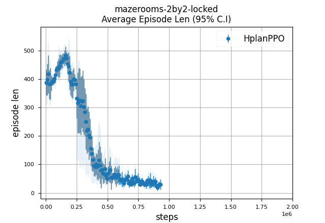
(a) Goal Option Episode Length

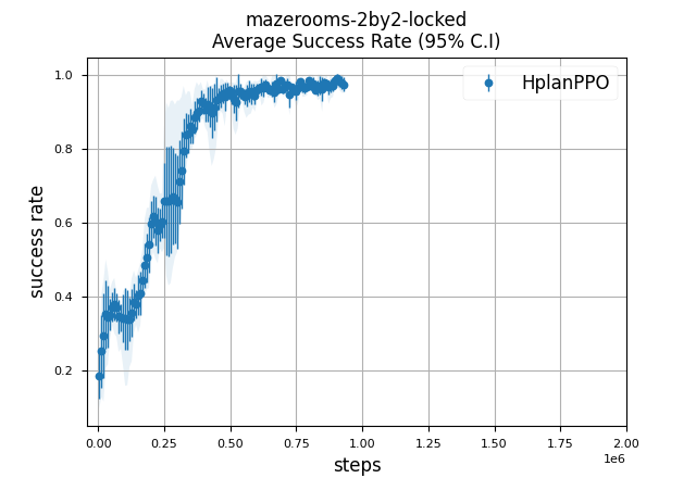
(b) Goal Option Success Rate

Figure 13: Option Learning Progress in MiniGrid 4 Rooms with a Locked Door Domain

Plan from Annotated Planning Task

state:0
(unlocked d-yellow-0-0-0-1)
(unlocked d-yellow-0-0-1-0)
(locked d-yellow-1-0-1-1)
(empty-hand)
(at k-yellow-0 r-1-0)
(at-agent r-0-0)

action:0
(move-room d-yellow-0-0-1-0 r-0-0 r-1-0)
  PRE: (unlocked d-yellow-0-0-1-0)
  PRE: (at-agent r-0-0)
  ADD: (at-agent r-1-0)
  DEL: (at-agent r-0-0)

state:1
(empty-hand)
(unlocked d-yellow-0-0-0-1)
(locked d-yellow-1-0-1-1)
(at-agent r-1-0)
(at k-yellow-0 r-1-0)
(unlocked d-yellow-0-0-1-0)

action:1
(pickup k-yellow-0 r-1-0)
  PRE: (at-agent r-1-0)
  PRE: (at k-yellow-0 r-1-0)
  PRE: (empty-hand)
  ADD: (carry k-yellow-0)
  DEL: (at k-yellow-0 r-1-0)
  DEL: (empty-hand)

state:2
(carry k-yellow-0)
(unlocked d-yellow-0-0-0-1)
(locked d-yellow-1-0-1-1)
(at-agent r-1-0)
(unlocked d-yellow-0-0-1-0)

action:2
(unlock k-yellow-0 d-yellow-1-0-1-1 r-1-0 r-1-1)
  PRE: (at-agent r-1-0)
  PRE: (carry k-yellow-0)
  PRE: (locked d-yellow-1-0-1-1)
  ADD: (unlocked d-yellow-1-0-1-1)
  DEL: (locked d-yellow-1-0-1-1)

state:3
(carry k-yellow-0)
(unlocked d-yellow-1-0-1-1)
(unlocked d-yellow-0-0-0-1)
(at-agent r-1-0)
(unlocked d-yellow-0-0-1-0)

action:3
(move-room d-yellow-1-0-1-1 r-1-0 r-1-1)
  PRE: (at-agent r-1-0)
  PRE: (unlocked d-yellow-1-0-1-1)
  ADD: (at-agent r-1-1)
  DEL: (at-agent r-1-0)

D.3 MiniGrid 9 Rooms with Locked Doors

Figure 14 – 15 show learning progress of options and we show a shortest plan from annotated planning task.

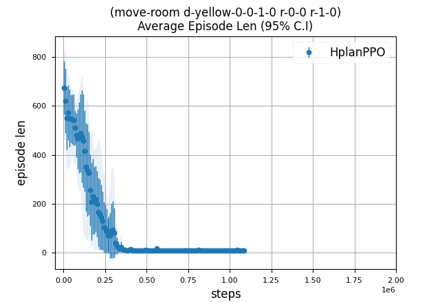
(a) (move-room d-yellow-0-0-1-0 r-0-0 r-1-0) Episode Length

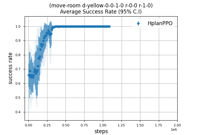
(b) (move-room d-yellow-0-0-1-0 r-0-0 r-1-0) Success Rate

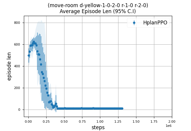
(c) (move-room d-yellow-1-0-2-0 r-1-0 r-2-0) Episode Length

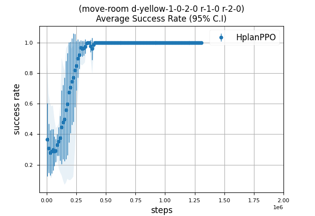
(d) (move-room d-yellow-1-0-2-0 r-1-0 r-2-0) Success Rate

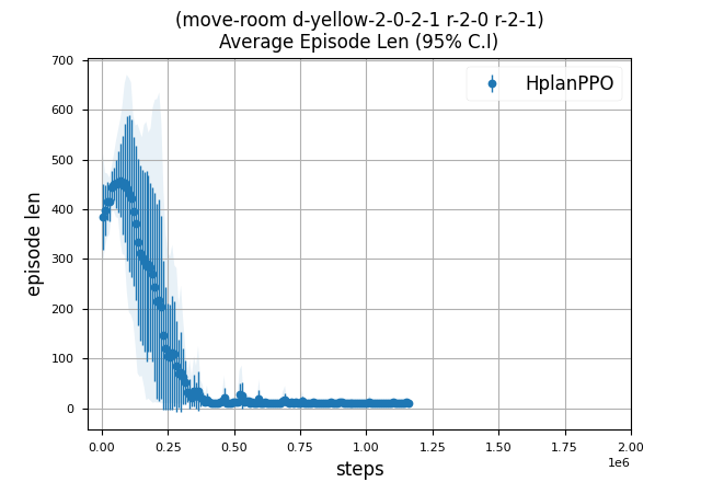
(e) (move-room d-yellow-2-0-2-1 r-2-0 r-2-1) Episode Length

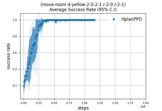
(f) (move-room d-yellow-2-0-2-1 r-2-0 r-2-1) Success Rate

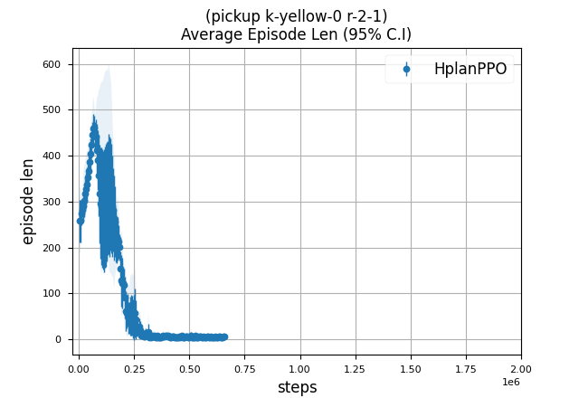
(g) (pickup k-yellow-0 r-2-1) Episode Length

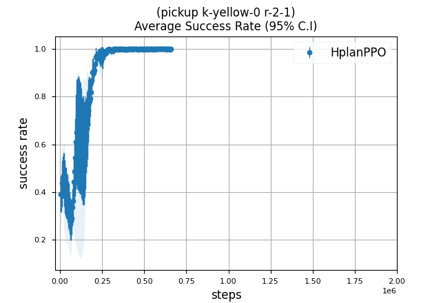
(h) (pickup k-yellow-0 r-2-1) Success Rate

Figure 14: Option Learning Progress in MiniGrid 9 Rooms with Locked Doors Domain

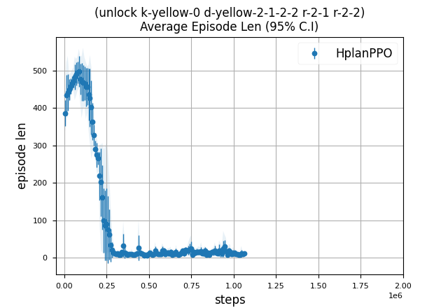
(a) (unlock k-yellow-0 d-yellow-2-1-2-2 r-2-1 r-2-2) Episode Length

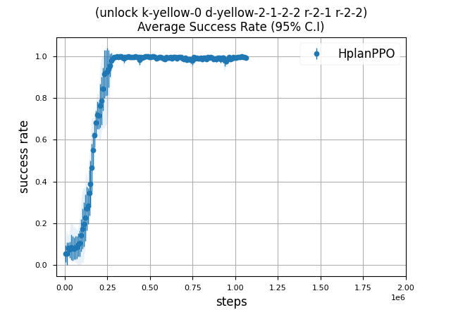
(b) (unlock k-yellow-0 d-yellow-2-1-2-2 r-2-1 r-2-2) Success Rate

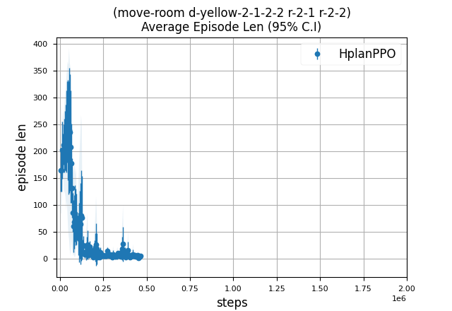
(c) (move-room d-yellow-2-1-2-2 r-2-1 r-2-2) Episode Length

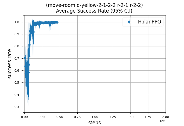
(d) (move-room d-yellow-2-1-2-2 r-2-1 r-2-2) Success Rate

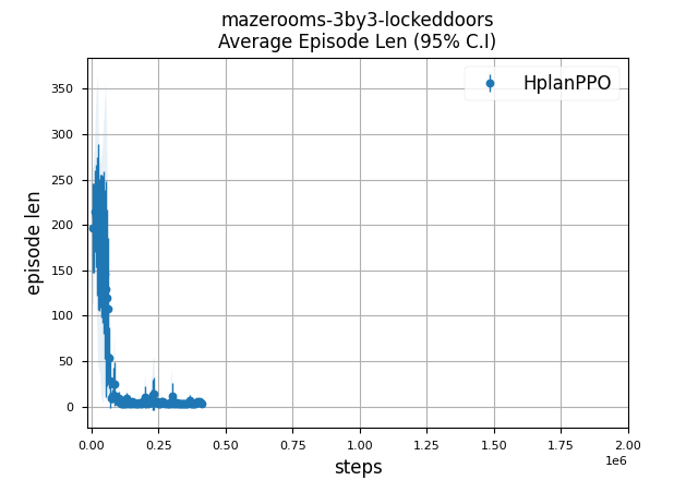
(e) Goal Option Episode Length

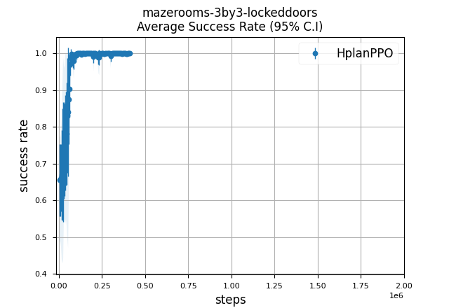
(f) Goal Option Success Rate

Figure 15: Option Learning Progress in MiniGrid 9 Rooms with Locked Doors Domain

Plan from Annotated Planning Task

state:0
(unlocked d-yellow-1-1-1-2)
(locked d-yellow-1-2-2-2)
(unlocked d-yellow-2-0-2-1)
(unlocked d-yellow-1-0-2-0)
(unlocked d-yellow-0-0-0-1)
(at k-yellow-0 r-2-1)
(locked d-yellow-0-1-1-1)
(unlocked d-yellow-0-0-1-0)
(locked d-yellow-1-0-1-1)
(unlocked d-yellow-0-1-0-2)
(unlocked d-yellow-0-2-1-2)
(locked d-yellow-2-1-2-2)
(empty-hand)
(unlocked d-yellow-1-1-2-1)
(at-agent r-0-0)

action:0
(move-room d-yellow-0-0-1-0 r-0-0 r-1-0)
  PRE: (unlocked d-yellow-0-0-1-0)
  PRE: (at-agent r-0-0)
  ADD: (at-agent r-1-0)
  DEL: (at-agent r-0-0)

state:1
(unlocked d-yellow-1-1-1-2)
(locked d-yellow-1-2-2-2)
(unlocked d-yellow-2-0-2-1)
(unlocked d-yellow-1-0-2-0)
(unlocked d-yellow-0-0-0-1)
(at-agent r-1-0)
(at k-yellow-0 r-2-1)
(locked d-yellow-0-1-1-1)
(unlocked d-yellow-0-0-1-0)
(unlocked d-yellow-0-1-0-2)
(unlocked d-yellow-0-2-1-2)
(locked d-yellow-2-1-2-2)
(empty-hand)
(locked d-yellow-1-0-1-1)
(unlocked d-yellow-1-1-2-1)

action:1
(move-room d-yellow-1-0-2-0 r-1-0 r-2-0)
  PRE: (at-agent r-1-0)
  PRE: (unlocked d-yellow-1-0-2-0)
  ADD: (at-agent r-2-0)
  DEL: (at-agent r-1-0)

state:2
(unlocked d-yellow-1-1-1-2)
(locked d-yellow-1-2-2-2)
(unlocked d-yellow-2-0-2-1)
(unlocked d-yellow-1-0-2-0)
(unlocked d-yellow-0-0-0-1)
(at k-yellow-0 r-2-1)
(locked d-yellow-0-1-1-1)
(unlocked d-yellow-0-0-1-0)
(locked d-yellow-1-0-1-1)
(unlocked d-yellow-0-1-0-2)
(unlocked d-yellow-0-2-1-2)
(locked d-yellow-2-1-2-2)
(at-agent r-2-0)
(empty-hand)
(unlocked d-yellow-1-1-2-1)

action:2
(move-room d-yellow-2-0-2-1 r-2-0 r-2-1)
  PRE: (unlocked d-yellow-2-0-2-1)
  PRE: (at-agent r-2-0)
  ADD: (at-agent r-2-1)
  DEL: (at-agent r-2-0)

state:3
(unlocked d-yellow-1-1-1-2)
(locked d-yellow-1-2-2-2)
(unlocked d-yellow-2-0-2-1)
(unlocked d-yellow-1-0-2-0)
(unlocked d-yellow-0-0-0-1)
(at-agent r-2-1)
(at k-yellow-0 r-2-1)
(locked d-yellow-0-1-1-1)
(unlocked d-yellow-0-0-1-0)
(unlocked d-yellow-0-1-0-2)
(unlocked d-yellow-0-2-1-2)
(locked d-yellow-2-1-2-2)
(empty-hand)
(locked d-yellow-1-0-1-1)
(unlocked d-yellow-1-1-2-1)

action:3
(pickup k-yellow-0 r-2-1)
  PRE: (at k-yellow-0 r-2-1)
  PRE: (empty-hand)
  PRE: (at-agent r-2-1)
  ADD: (carry k-yellow-0)
  DEL: (at k-yellow-0 r-2-1)
  DEL: (empty-hand)

state:4
(carry k-yellow-0)
(unlocked d-yellow-1-1-1-2)
(locked d-yellow-1-2-2-2)
(unlocked d-yellow-2-0-2-1)
(unlocked d-yellow-1-0-2-0)
(unlocked d-yellow-0-0-0-1)
(at-agent r-2-1)
(locked d-yellow-0-1-1-1)
(unlocked d-yellow-0-0-1-0)
(unlocked d-yellow-0-1-0-2)
(unlocked d-yellow-0-2-1-2)
(locked d-yellow-2-1-2-2)
(locked d-yellow-1-0-1-1)
(unlocked d-yellow-1-1-2-1)

action:4
(unlock k-yellow-0 d-yellow-2-1-2-2 r-2-1 r-2-2)
  PRE: (carry k-yellow-0)
  PRE: (locked d-yellow-2-1-2-2)
  PRE: (at-agent r-2-1)
  ADD: (unlocked d-yellow-2-1-2-2)
  DEL: (locked d-yellow-2-1-2-2)

state:5
(carry k-yellow-0)
(unlocked d-yellow-1-1-1-2)
(locked d-yellow-1-2-2-2)
(unlocked d-yellow-2-0-2-1)
(unlocked d-yellow-1-0-2-0)
(unlocked d-yellow-0-0-0-1)
(at-agent r-2-1)
(locked d-yellow-0-1-1-1)
(unlocked d-yellow-0-0-1-0)
(unlocked d-yellow-2-1-2-2)
(unlocked d-yellow-0-1-0-2)
(unlocked d-yellow-0-2-1-2)
(locked d-yellow-1-0-1-1)
(unlocked d-yellow-1-1-2-1)

action:5
(move-room d-yellow-2-1-2-2 r-2-1 r-2-2)
  PRE: (unlocked d-yellow-2-1-2-2)
  PRE: (at-agent r-2-1)
  ADD: (at-agent r-2-2)
  DEL: (at-agent r-2-1)

D.4 Other Algorithms

For other algorithms HplanDDQN and HRM, we tried hyperparameter tuning for DDQN and tested with CNN and Flattened observation feature extractors. HRM was able to solve MiniGrid DoorKey environment, but it couldn’t solve larger domains. HplanDDQN was not able to solve any MiniGrid-based domains. Both HRM and HplanDDQN have the same neural network architecture, but the main difference between HRM and HplanDDQN is that HplanDDQN did not reuse samples across options.

References

- Abdulhai et al. (2022) Abdulhai, M.; Kim, D.-K.; Riemer, M.; Liu, M.; Tesauro, G.; and How, J. P. 2022. Context-Specific Representation Abstraction for Deep Option Learning. In Honavar, V.; and Spaan, M., eds., Proceedings of the AAAI Conference on Artificial Intelligence, 5959–5967. AAAI Press.
- Alkhazraji et al. (2016) Alkhazraji, Y.; Frorath, M.; Grützner, M.; Liebetraut, T.; Ortlieb, M.; Seipp, J.; Springenberg, T.; Stahl, P.; Wülfing, J.; Helmert, M.; et al. 2016. Pyperplan.
- Araki et al. (2021) Araki, B.; Li, X.; Vodrahalli, K.; DeCastro, J.; Fry, M. J.; and Rus, D. 2021. The Logical Options Framework. arXiv preprint arXiv:2102.12571.
- Bäckström and Nebel (1995) Bäckström, C.; and Nebel, B. 1995. Complexity Results for SAS+ Planning. Computational Intelligence, 11(4): 625–655.
- Bacon, Harb, and Precup (2017) Bacon, P.; Harb, J.; and Precup, D. 2017. The Option-Critic Architecture. In Singh, S.; and Markovitch, S., eds., Proceedings of the Thirty-First AAAI Conference on Artificial Intelligence (AAAI 2017), 1726–1734. AAAI Press.
- Bagaria and Konidaris (2019) Bagaria, A.; and Konidaris, G. 2019. Option discovery using deep skill chaining. In Proceedings of the Seventh International Conference on Learning Representations(ICLR 2019).
- Barto and Mahadevan (2003) Barto, A. G.; and Mahadevan, S. 2003. Recent advances in hierarchical reinforcement learning. 13(1): 41–77.
- Bertsekas (2018) Bertsekas, D. 2018. Abstract dynamic programming. Athena Scientific.
- Camacho et al. (2019) Camacho, A.; Icarte, R. T.; Klassen, T. Q.; Valenzano, R. A.; and McIlraith, S. A. 2019. LTL and Beyond: Formal Languages for Reward Function Specification in Reinforcement Learning. In IJCAI, volume 19, 6065–6073.
- Castro and Precup (2011) Castro, P. S.; and Precup, D. 2011. Automatic construction of temporally extended actions for mdps using bisimulation metrics. In European Workshop on Reinforcement Learning, 140–152. Springer.
- Chevalier-Boisvert et al. (2019) Chevalier-Boisvert, M.; Bahdanau, D.; Lahlou, S.; Willems, L.; Saharia, C.; Nguyen, T. H.; and Bengio, Y. 2019. BabyAI: First Steps Towards Grounded Language Learning With a Human In the Loop. In International Conference on Learning Representations.
- Chevalier-Boisvert, Willems, and Pal (2018) Chevalier-Boisvert, M.; Willems, L.; and Pal, S. 2018. Minimalistic Gridworld Environment for OpenAI Gym. https://github.com/maximecb/gym-minigrid.
- Dayan and Hinton (1992) Dayan, P.; and Hinton, G. E. 1992. Feudal Reinforcement Learning. In Proceedings of the Fourth Annual Conference on Neural Information Processing Systems (NIPS 1992), 271–278.
- Dean and Lin (1995) Dean, T.; and Lin, S.-H. 1995. Decomposition techniques for planning in stochastic domains. In IJCAI, volume 2, 3.
- Den Hengst et al. (2022) Den Hengst, F.; François-Lavet, V.; Hoogendoorn, M.; and van Harmelen, F. 2022. Reinforcement Learning with Option Machines. In Proceedings of the Thirty-First International Joint Conference on Artificial Intelligence, IJCAI-22, 2909–2915. International Joint Conferences on Artificial Intelligence Organization.
- Eppe, Nguyen, and Wermter (2019) Eppe, M.; Nguyen, P. D.; and Wermter, S. 2019. From semantics to execution: Integrating action planning with reinforcement learning for robotic causal problem-solving. Frontiers in Robotics and AI, 6: 123.
- Garrett et al. (2021) Garrett, C. R.; Chitnis, R.; Holladay, R.; Kim, B.; Silver, T.; Kaelbling, L. P.; and Lozano-Pérez, T. 2021. Integrated task and motion planning. 4: 265–293.
- Gehring et al. (2021) Gehring, C.; Asai, M.; Chitnis, R.; Silver, T.; Kaelbling, L. P.; Sohrabi, S.; and Katz, M. 2021. Reinforcement Learning for Classical Planning: Viewing Heuristics as Dense Reward Generators. Planning and Reinforcement Learning PRL Workshop at ICAPS.
- Groshev et al. (2018) Groshev, E.; Tamar, A.; Goldstein, M.; Srivastava, S.; and Abbeel, P. 2018. Learning generalized reactive policies using deep neural networks. In 2018 AAAI Spring Symposium Series.
- Icarte et al. (2018) Icarte, R. T.; Klassen, T.; Valenzano, R.; and McIlraith, S. 2018. Using reward machines for high-level task specification and decomposition in reinforcement learning. In International Conference on Machine Learning, 2107–2116. PMLR.
- Icarte et al. (2022) Icarte, R. T.; Klassen, T. Q.; Valenzano, R.; and McIlraith, S. A. 2022. Reward machines: Exploiting reward function structure in reinforcement learning. Journal of Artificial Intelligence Research, 73: 173–208.
- Illanes et al. (2020) Illanes, L.; Yan, X.; Icarte, R. T.; and McIlraith, S. A. 2020. Symbolic Plans as High-Level Instructions for Reinforcement Learning. In Beck, J. C.; Karpas, E.; and Sohrabi, S., eds., Proceedings of the Thirtieth International Conference on Automated Planning and Scheduling (ICAPS 2020), 540–550. AAAI Press.
- Jin et al. (2022) Jin, M.; Ma, Z.; Jin, K.; Zhuo, H. H.; Chen, C.; and Yu, C. 2022. Creativity of AI: Automatic Symbolic Option Discovery for Facilitating Deep Reinforcement Learning. In Proceedings of the AAAI Conference on Artificial Intelligence, volume 36, 7042–7050.
- Kokel et al. (2021a) Kokel, H.; Manoharan, A.; Natarajan, S.; Balaraman, R.; and Tadepalli, P. 2021a. RePReL: Integrating Relational Planning and Reinforcement Learning for Effective Abstraction. Proceedings of the International Conference on Automated Planning and Scheduling, 31(1): 533–541.
- Kokel et al. (2021b) Kokel, H.; Manoharan, A.; Natarajan, S.; Ravindran, B.; and Tadepalli, P. 2021b. Deep RePReL–Combining Planning and Deep RL for acting in relational domains. In Deep RL Workshop NeurIPS 2021.
- Kolobov, Mausam, and Weld (2012) Kolobov, A.; Mausam; and Weld, D. 2012. A Theory of Goal-oriented MDPs with Dead Ends. In Proceedings of the 28th Conference on Uncertainty in Artificial Intelligence (UAI 2012), 438–447.
- Kulkarni et al. (2016) Kulkarni, T. D.; Narasimhan, K.; Saeedi, A.; and Tenenbaum, J. 2016. Hierarchical deep reinforcement learning: Integrating temporal abstraction and intrinsic motivation. In Proceedings of the Thirty Annual Conference on Neural Information Processing Systems (NIPS 2016), 3675–3683.
- Li, Walsh, and Littman (2006) Li, L.; Walsh, T. J.; and Littman, M. L. 2006. Towards a Unified Theory of State Abstraction for MDPs. ISAIM, 4: 5.
- Lyu et al. (2019) Lyu, D.; Yang, F.; Liu, B.; and Gustafson, S. 2019. SDRL: Interpretable and Data-efficient Deep Reinforcement Learning Leveraging Symbolic Planning. In Proceedings of the Thirty-Third AAAI Conference on Artificial Intelligence (AAAI 2019), 2970–2977. AAAI Press.
- Machado, Bellemare, and Bowling (2017) Machado, M. C.; Bellemare, M. G.; and Bowling, M. 2017. A Laplacian Framework for Option Discovery in Reinforcement Learning. In Proceedings of the Thirty-Fourth International Conference on Machine Learning (ICML 2017), 2295–2304.
- Mausam and Kolobov (2012) Mausam; and Kolobov, A. 2012. Planning with Markov Decision Processes: An AI Perspective. Synthesis Lectures on Artificial Intelligence and Machine Learning. Morgan & Claypool Publishers.
- McGovern and Barto (2001) McGovern, A.; and Barto, A. G. 2001. Automatic discovery of subgoals in reinforcement learning using diverse density. Computer Science Department Faculty Publication Series.
- Mnih et al. (2015) Mnih, V.; Kavukcuoglu, K.; Silver, D.; Rusu, A. A.; Veness, J.; Bellemare, M. G.; Graves, A.; Riedmiller, M.; Fidjeland, A. K.; Ostrovski, G.; et al. 2015. Human-level control through deep reinforcement learning. nature, 518(7540): 529–533.
- Nachum et al. (2018) Nachum, O.; Gu, S. S.; Lee, H.; and Levine, S. 2018. Data-Efficient Hierarchical Reinforcement Learning. Advances in Neural Information Processing Systems, 31: 3303–3313.
- Parr and Russell (1998) Parr, R.; and Russell, S. 1998. Reinforcement learning with hierarchies of machines. In Proceedings of the Twelfth Annual Conference on Neural Information Processing Systems (NIPS 1998), 1043–1049.
- Porteous, Sebastia, and Hoffmann (2001) Porteous, J.; Sebastia, L.; and Hoffmann, J. 2001. On the Extraction, Ordering, and Usage of Landmarks in Planning. In Cesta, A.; and Borrajo, D., eds., Proceedings of the Sixth European Conference on Planning (ECP 2001), 174–182. AAAI Press.
- Raffin et al. (2021) Raffin, A.; Hill, A.; Gleave, A.; Kanervisto, A.; Ernestus, M.; and Dormann, N. 2021. Stable-Baselines3: Reliable Reinforcement Learning Implementations. Journal of Machine Learning Research, 22(268): 1–8.
- Ravindran and Barto (2004) Ravindran, B.; and Barto, A. 2004. Approximate Homomorphisms : A framework for non-exact minimization in Markov Decision Processes. In Proceedings of the International Conference on Knowledge Based Computer Systems (KBCS 2004).
- Schulman et al. (2017) Schulman, J.; Wolski, F.; Dhariwal, P.; Radford, A.; and Klimov, O. 2017. Proximal Policy Optimization Algorithms. CoRR, abs/1707.06347.
- Shen, Trevizan, and Thiébaux (2020) Shen, W.; Trevizan, F.; and Thiébaux, S. 2020. Learning Domain-Independent Planning Heuristics with Hypergraph Networks. In Beck, J. C.; Karpas, E.; and Sohrabi, S., eds., Proceedings of the Thirtieth International Conference on Automated Planning and Scheduling (ICAPS 2020), 574–584. AAAI Press.
- Simsek and Barreto (2008) Simsek, O.; and Barreto, A. S. 2008. Skill characterization based on betweenness. In Proceedings of the Twenty-second Annual Conference on Neural Information Processing Systems (NIPS 2008), 1497–1504.
- Singh, Barto, and Chentanez (2004) Singh, S.; Barto, A. G.; and Chentanez, N. 2004. Intrinsically motivated reinforcement learning. In Proceedings of the Eighteenth Annual Conference on Neural Information Processing Systems (NIPS 2004), 1281–1288.
- Stolle and Precup (2002) Stolle, M.; and Precup, D. 2002. Learning Options in Reinforcement Learning. In Koenig, S.; and Holte, R. C., eds., Proceedings of the 5th International Symposium on Abstraction, Reformulation and Approximation (SARA 2002), volume 2371 of Lecture Notes in Artificial Intelligence, 212–223. Springer-Verlag.
- Sutton and Barto (1998) Sutton, R. S.; and Barto, A. G. 1998. Reinforcement Learning: An Introduction. Cambridge, MA, USA: MIT Press.
- Sutton, Precup, and Singh (1999) Sutton, R. S.; Precup, D.; and Singh, S. P. 1999. Between MDPs and Semi-MDPs: A Framework for Temporal Abstraction in Reinforcement Learning. Artificial Intelligence, 112(1-2): 181–211.
- Toyer et al. (2018) Toyer, S.; Trevizan, F.; Thiébaux, S.; and Xie, L. 2018. Action Schema Networks: Generalised Policies with Deep Learning. In Proceedings of the Thirty-Second AAAI Conference on Artificial Intelligence (AAAI 2018), 6294–6301. AAAI Press.
- Van Hasselt, Guez, and Silver (2016) Van Hasselt, H.; Guez, A.; and Silver, D. 2016. Deep reinforcement learning with double q-learning. In Proceedings of the AAAI conference on artificial intelligence, volume 30.
- Vezhnevets et al. (2017) Vezhnevets, A. S.; Osindero, S.; Schaul, T.; Heess, N.; Jaderberg, M.; Silver, D.; and Kavukcuoglu, K. 2017. Feudal networks for hierarchical reinforcement learning. In Proceedings of the Thirty-Fourth International Conference on Machine Learning (ICML 2017), 3540–3549.
- Watkins and Dayan (1992) Watkins, C. J.; and Dayan, P. 1992. Q-learning. Machine learning, 8(3–4): 279–292.
- Wen et al. (2020) Wen, Z.; Precup, D.; Ibrahimi, M.; Barreto, A.; Van, B. R.; and Singh, S. 2020. On Efficiency in Hierarchical Reinforcement Learning. In Proceedings of the Thirty-fourth Annual Conference on Neural Information Processing Systems (NeurIPS 2020), 6708–6718.
- Yang, Littman, and Carbin (2022) Yang, C.; Littman, M. L.; and Carbin, M. 2022. On the (In) Tractability of Reinforcement Learning for LTL Objectives. In Proceedings of the Thirty-First International Joint Conference on Artificial Intelligence (IJCAI).
- Yang et al. (2018) Yang, F.; Lyu, D.; Liu, B.; and Gustafson, S. 2018. PEORL: Integrating Symbolic Planning and Hierarchical Reinforcment Learning for Robust Decision-Making. In Lang, J., ed., Proceedings of the 27th International Joint Conference on Artificial Intelligence (IJCAI 2018), 4860–4866. IJCAI.