Information back-flow in quantum non-Markovian dynamics and its connection to teleportation

Abstract

A quantum process is called non-Markovian when memory effects take place during its evolution. Quantum non-Markovianity is a phenomenon typically associated with the information back-flow from the environment to the principal system, however it has been shown that such an effect is not necessary. In this work, we establish a connection between quantum non-Markovianity and the protocol of quantum teleportation in both discrete and continuous-variable systems. We also show how information flows during a teleportation protocol between the principal system and the environment in a bidirectional way leading up to a state revival. Finally, given the resource-like role of entanglement in the teleportation protocol, the relationship between this property and non-Markovianity is also elucidated.

I Introduction

Markovianity [1] refers to stochastic processes where the past of the system can influence its future only through its present state. Otherwise, the process is called non-Markovian, and can be interpreted as if the system contains a memory. Given that quantum mechanics is an inherently statistical theory, Markovian and non-Markovian phenomena naturally arise in quantum systems too [2, 3, 4, 5, 6, 7, 8, 9]. Even though non-Markovianity is typically associated with information flow from the principal system to the environment and back into the principal system [10, 11, 12], called information back-flow, it has been shown that this effect not only is not necessary [13, 14, 15], but maximal non-Markovianity, i.e., complete state revival, can be achieved in its absence [16, 17].

Teleportation is a non-classical application that is conventionally described through a measurement-based process [18, 19]. The information flow during the teleportation protocol has been initially discussed in Refs. [20, 21], but no connection was drawn to the concept of non-Markovianity. In this work, we show that the protocol of measurement-free teleportation (which is mathematically identical to the measurement-based protocol) is a time-homogeneous maximally non-Markovian process. In particular, we show this connection for both discrete-variable teleportation, which we extend from two-dimensional states [22] to finite-dimensional ones, and continuous-variable states [23]. We also show how the non-Markovian nature of teleportation is entirely based on an information back-flow effect, which can be explained through the more general observation that time-homogeneity is a sufficient condition for any state revival in a non-Markovian quantum process to originate from information back-flow. Finally, given that entanglement is considered the resource for the protocol of teleportation, the relationship between entanglement and non-Markovianity [24, 25, 26, 27, 28, 29, 30, 31] is explained through this resource-oriented perspective.

II Quantum Systems

Let $S$ be a a $d\times d$ density matrix representing a quantum state in the Hilbert space $\mathscr{H}_{d}^{(\mathrm{S})}$ [32, 33], belonging to the principal system. Due to the Stinespring dilation theorem [34], a completely-positive trace-preserving (CPTP) map ${\mathcal{M}}:\mathscr{H}_{d}^{(\mathrm{S})}\rightarrow\mathscr{H}_{d}^{(\mathrm{S})}$ can be written as

$${\mathcal{M}}(S)=\mathrm{tr}_{\mathrm{E}}\left[\mathit{U}(t)(S\otimes\mathit{E})\mathit{U}^{{\dagger}}(t)\right],$$ (1)

where: (i) $\mathit{E}\in\mathscr{H}_{d}^{(\mathrm{E})}$ denotes a quantum state that belongs to the environment; (ii) $\mathit{U}(t)={\mathcal{T}}\big{[}e^{\int_{t_{a}}^{t_{b}}\differential t\mathit{L}(t)}\big{]}\in\mathscr{H}_{d}^{(\mathrm{S})}{\otimes}\mathscr{H}_{d}^{(\mathrm{E})}$ is a unitary operator associated with the interaction between the principal system and the environment, with ${\mathcal{T}}$ being the chronological time-ordering superoperator, $\tau=t_{b}-t_{a}$ the time period within which the interaction takes place, and $\mathit{L}(t)$ the generator operator; and (iii) $\mathrm{tr}_{\mathrm{E}}$ is the partial trace over $\mathscr{H}_{d}^{(\mathrm{E})}$. When the generator depends explicitly on time the quantum process is called time-inhomogeneous, otherwise, when $\mathit{L}(t)=\mathit{L}\Rightarrow\mathit{U}(t)=\mathit{U}=e^{\tau\mathit{L}}$ the quantum process is called time-homogeneous, and depends only on $\tau$.

The quantum evolution in Eq. (1) can take the equivalent operator-sum representation [35, 36]

$${\mathcal{M}}(S)=\sum_{i}\mathit{F}_{i}(t)S\mathit{F}_{i}^{{\dagger}}(t),$$ (2)

where the set of operators $\mathbbol{F}\equiv\{\mathit{F}_{i}(t)\}$ are known as Kraus operators, satisfying $\sum_{i}\mathit{F}_{i}^{{\dagger}}(t)\mathit{F}_{i}(t)=\mathds{1}$. For a subset of CPTP maps, e.g., qubit channels, Eq. (2) can be written in terms of a probability distribution $\mathbbol{P}\equiv\{p_{i}(t)\}$ and a set of unitary operators $\mathbbol{U}\equiv\{\mathit{U}_{i}(t)\}$,

$${\mathcal{M}}(S)=\sum_{i}p_{i}(t)\mathit{U}_{i}(t)S\mathit{U}_{i}^{{\dagger}}(t).$$ (3)

The above CPTP maps, that are referred to as mixed-unitary [37, 38], admit an interesting interpretation, since the principal system and the environment seem to be evolving without affecting each other.

III Quantum Markovianity

Markovianity in quantum systems admits various definitions [2, 3, 4, 5, 6, 7, 8, 9]. Here, we follow Ref. [24], and call a quantum process Markovian if its corresponding CPTP map ${\mathcal{M}}$ is divisible. A CPTP map that takes place during a time interval $(t_{0},t_{n})$, with $n\in\mathbbol{N}$ and $t_{0}<t_{n}$, is called divisible if it can be written as the concatenation of the CPTP maps of each time sub-interval, i.e.,

$${\mathcal{M}}_{(t_{0},t_{n})}={\mathcal{M}}_{(t_{n-1},t_{n})}\circ\cdots\circ{\mathcal{M}}_{(t_{1},t_{2})}\circ{\mathcal{M}}_{(t_{0},t_{1})},$$ (4)

with $t_{0}<t_{1}<\cdots<t_{n}$, assuming that the environment state $\mathit{E}$ associated to the CPTP map of each sub-interval is the same fixed quantum state. This assumption guarantees the memoryless (Markovian) nature of the quantum system by not allowing $\mathit{E}$ to carry any system-environment correlations from past interactions. The divisible process in Eq. (4) for $n=2$ is depicted in Fig. 1, where the system is coupled to the environment through two subsequent unitary transformations and the environment states are traced out after each transformation. When a quantum process is not divisible it is called non-Markovian. Experimentally, non-Markovianity can be simulated through different platforms, such as optical systems [39, 40, 41, 42, 43, 44], trapped ions [45], NMR [46], and quantum computers [47, 48, 49, 50].

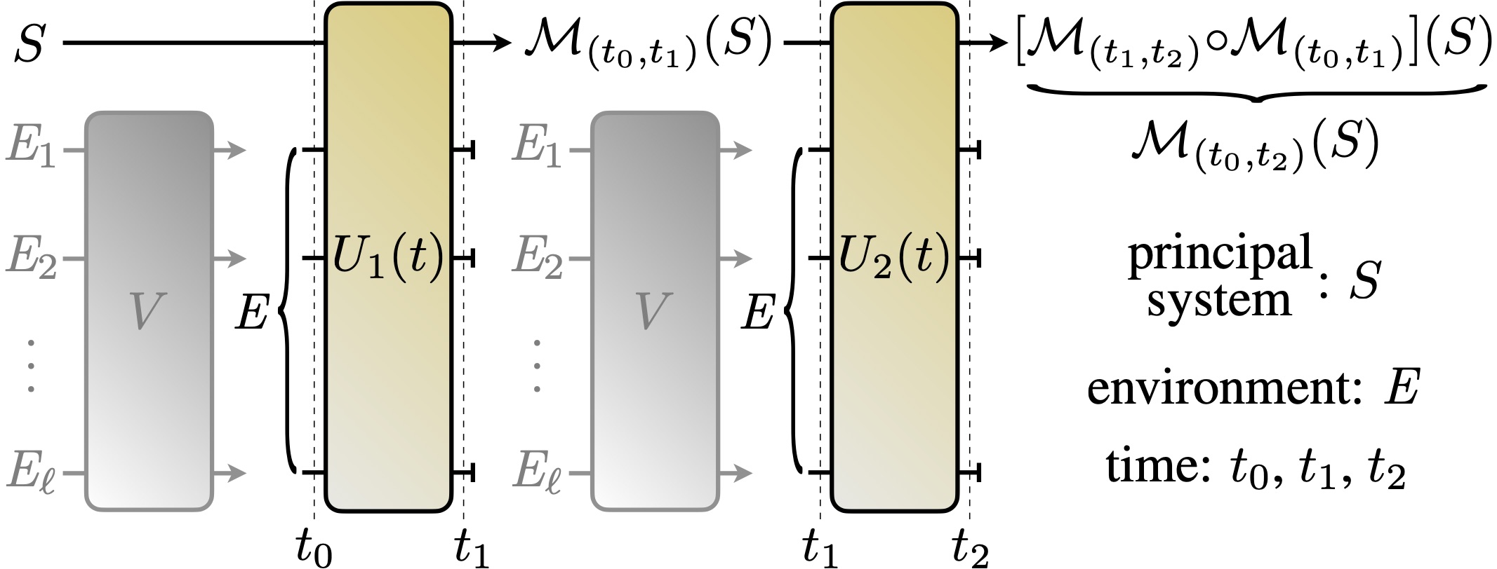
Figure 1: Markovian system. During the time interval $(t_{0},t_{1})$ the quantum state $S$ is coupled to the environment, $\mathit{E}$, through a unitary operation $\mathit{U}_{1}(t)$. $\mathit{E}$ is in general an ensemble of states $\mathbbol{E}=\{\mathit{E}_{1},\mathit{E}_{2},\cdots,\mathit{E}_{\ell}\}$ coupled with each other through a unitary operation $\mathit{V}$. After this interaction all environment states are discarded, and the output state is ${\mathcal{M}}_{(t_{0},t_{1})}(S)$. During the time interval $(t_{1},t_{2})$, the state ${\mathcal{M}}_{(t_{0},t_{1})}(S)$ is coupled again with $\mathit{E}$ through a unitary operation $\mathit{U}_{2}(t)$, and upon discarding the interacted environment states the output final state is $[{\mathcal{M}}_{(t_{1},t_{2})}{\circ}{\mathcal{M}}_{(t_{0},t_{1})}](S)$=${\mathcal{M}}_{(t_{0},t_{2})}(S)$.

IV Information back-flow effect

A revival of a state in the principal system during its evolution through a quantum process is a sufficient (but not necessary) condition to detect non-Markovianity [3], which can be checked through the non-monotonous behavior of the distinguishability between two evolving quantum states. In Refs. [10, 11, 12] this non-monotonous behavior of distinguishability was attributed to the back-flow of information from the environment to the principal system, however it was later shown [13, 14, 15, 16, 17] that the two concepts are not always equivalent. In particular, a time-inhomogeneous non-Markovian process that evolves according to Eq. (3) can revive a quantum state without any information back-flow effect . This is possible since in time-inhomogeneous processes the generators $\mathit{L}(t)$ evolve along with the system, and thus, this time-dependency must originate from an external to the total system (principal system and environment) source, i.e., the total system is not closed. On the other hand, in time-homogeneous processes the generators are time-independent, so the total system is closed [32, 33], which implies that any state revival must originate from information back-flow due to the conservation of quantum information principle [52] . Note that a state revival is impossible if a quantum process is described by a time-independent mixed-unitary map of the from of Eq. (3), since then the evolution of the principal system effectively reduces to a single unitary transformation , which means that there is no external influence to the principal system.

Below, we show that the teleportation protocol corresponds to a maximally non-Markovian time-homogeneous quantum process.

V Teleportation

In general, any teleportation protocol involves two agents, called Alice and Bob. Alice has an input state $S$ that wants to send to Bob. The two agents also share a bipartite entangled state $\mathit{R}$, known as the resource state, and a perfect teleportation requires a maximally entangled resource state, given by $\mathit{R}=\varPhi=\outerproduct{\phi}{\phi}$, with $\ket{\phi}=\frac{1}{\sqrt{d}}\sum_{i=0}^{d-1}\ket{ii}$, where $d$ denotes the dimensions of the Hilbert space, and $\{\ket{i}\}_{i=0}^{d-1}$ an orthonormal basis. Note that $\ket{ii}\equiv\ket{i}{\otimes}\ket{i}$.

Let us consider the measurement-free teleportation protocol [22, 23] which is a modified version of the conventional (measurement-based) teleportation [18, 19]. This protocol can be summarized as the process where at Alice’s side the input state $S$ is coupled to an entangled state $\mathit{R}$. The outcome of this interaction is sent to Bob coherently, where the input state $S$ is recovered via another interaction.

V.1 Discrete-variable Teleportation

Measurement-free teleportation in discrete-variable (DV) systems was introduced by Brassard, Braunstein, and Cleve (BBC) for 2-dimensional states, i.e., qubits [22] and it was experimentally realized for the first time in Ref. [53]. The BBC protocol requires the use of two quantum gates: (i) the Hadamard and (ii) the controlled-NOT (CNOT). For the purposes of this work the SWAP gate is also used in order the final state to appear in the principal system. Note that the Hilbert space on which the recovered state appears is irrelevant since Bob has access to all of them. This modified version of the BCC protocol is depicted in Fig. 2 (a).

Here, we extend the BBC protocol in arbitrary finite $d$-dimensional states, i.e., qudits. In order to do so, the aforementioned quantum gates need to be appropriately generalized. The generalized Hadamard gate corresponds to the discrete Fourier transform $\mathrm{H}(\theta)\ket{j}\coloneqq\frac{1}{\sqrt{d}}\sum_{i=0}^{d-1}e^{\frac{ij\theta\imath}{d}}\ket{i}$, where $\{\ket{i}\}_{i=0}^{d-1}$ and $\{\ket{j}\}_{j=0}^{d-1}$ are orthonormal bases, $\theta\in[0,2d\pi]$, and $\imath\coloneqq\sqrt{-1}$. The generalized CNOT gate can be defined as $\mathrm{CNOT}(\varphi,\theta)\ket{ij}\coloneqq[\mathds{1}{\otimes}\mathrm{H}(\theta)]\mathrm{CPhase}(\varphi)[\mathds{1}{\otimes}\mathrm{H}(\theta)]\ket{ij}$[54], where $\mathrm{CPhase}(\varphi)\ket{ij}\coloneqq e^{\frac{ij\varphi\imath}{d}}\ket{ij}$ is the generalized controlled-phase (CPhase) gate with $\varphi\in[0,2d\pi]$ . Finally, the generalized SWAP gate, $\mathrm{SWAP}(\varphi,\theta)$, is constructed through a sequence of three generalized CNOT gates where the middle one is inverted [54], as shown in Fig. 2 (c).

Let $S\in\mathscr{H}^{(\mathrm{S})}_{d}$ be an arbitrary quantum state belonging to Alice, and $\mathit{E}_{1}{\otimes}\mathit{E}_{2}=\outerproduct{00}{00}\in\mathscr{H}^{(\mathrm{E}_{1})}_{d}{\otimes}\mathscr{H}^{(\mathrm{E}_{2})}_{d}$ are two fixed pure states belonging to the environment. Note that by “environment” here we do not refer to an unknown (beyond our control) system that is typically assumed in open-quantum system scenarios, but to the system that we trace out after the interaction takes place. The DV measurement-free teleportation can be realized through the following non-divisible operation

$$\mathrm{tr}_{\mathrm{E_{1,2}}}\left[\mathit{U}_{3}\mathit{U}_{2}\mathit{U}_{1}(S\otimes\mathit{E}_{1}\otimes\mathit{E}_{2})\mathit{U}^{{\dagger}}_{1}\mathit{U}^{{\dagger}}_{2}\mathit{U}^{{\dagger}}_{3}\right]=S,$$ (5)

where

$$\mathit{U}_{1} =[\mathds{1}\otimes\mathrm{CNOT}(2\pi,2d\pi{-}2\pi)][\mathds{1}\otimes\mathrm{H}(2\pi)\otimes\mathds{1}],$$ (6a)

$$\mathit{U}_{2} =[\mathrm{H}(2\pi)\otimes\mathds{1}\otimes\mathds{1}][\mathrm{CNOT}(2\pi,2d\pi{-}2\pi)\otimes\mathds{1}],$$ (6b)

$$\mathit{U}_{3} =[\mathrm{SWAP}(2\pi,2\pi)\otimes\mathds{1}]$$

$$\hskip 13.08846pt{\times}[\mathds{1}\otimes\mathrm{H}(2\pi)\otimes\mathds{1}][\mathrm{CNOT}(2\pi,2\pi)\otimes\mathds{1}]$$

$$\hskip 13.08846pt{\times}[\mathds{1}\otimes\mathrm{SWAP}(2\pi,2\pi)]$$

$$\hskip 13.08846pt{\times}[\mathds{1}\otimes\mathds{1}\otimes\mathrm{H}(2d\pi{-}2\pi)][\mathds{1}\otimes\mathrm{CNOT}(2\pi,2\pi)].$$ (6c)

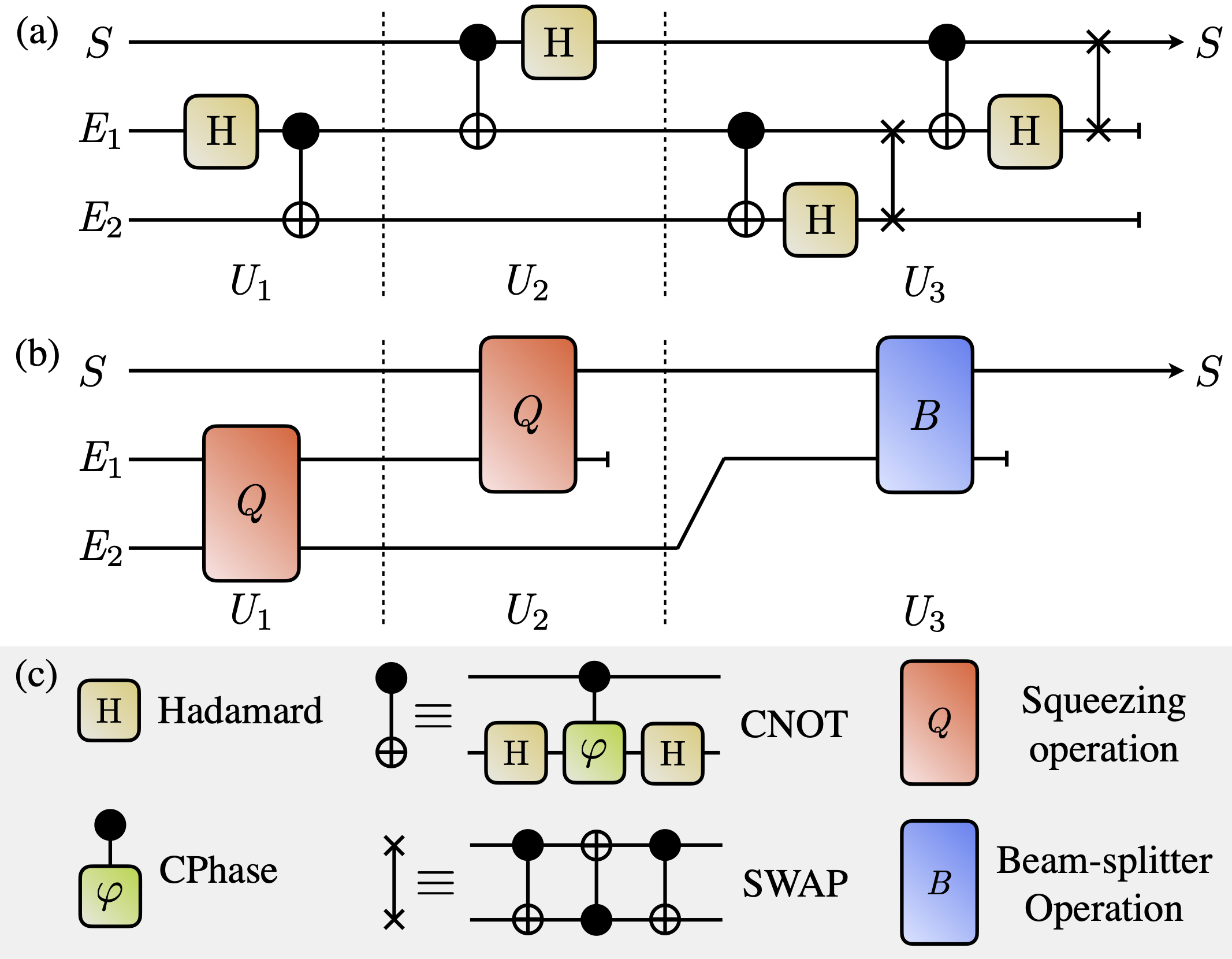
Figure 2: Measurement-free teleportation circuits. In panel (a) the DV teleportation is presented, and in panel (b) the CV one. The dashed lines in each panel denote the three subsequent operations of the protocols, $\mathit{U}_{1}$, $\mathit{U}_{2}$, and $\mathit{U}_{3}$. In panel (c) the gates and operations used in the circuits are labeled. The specific parameters used in the gate and operations above are given in Eq. (6) and Eq. (11).

In order to see how information flows from one system to another, let us consider for simplicity a pure state $\ket{s}$ for the principal system and two fixed pure states $\ket{00}$ for the environment. During the first stage, $\mathit{U}_{1}$, the two states in the environment become maximally entangled,

$$\mathit{U}_{1}\left(\ket{s}\otimes\ket{00}\right)=\ket{s}\otimes\ket{\phi}.$$ (7)

The next stage, $\mathit{U}_{2}$, corresponds to the coupling between the principal state and the environment, that effectively leads to information about the state $\ket{s}$ moving from $\mathscr{H}^{(\mathrm{S})}$ to $\mathscr{H}^{(\mathrm{E}_{2})}$, described by the identity [57, 58],

$$\mathit{U}_{2}(\ket{s}\otimes\ket{\phi})=\frac{1}{d}\sum_{i,j=0}^{d-1}\ket{ij}\otimes\mathit{X}_{d}^{d-j}\mathit{Z}_{d}^{i}\ket{s},$$ (8)

where $\mathit{X}_{d}=\sum_{i=0}^{d-1}\outerproduct{i\oplus 1}{i}$ and $\mathit{Z}_{d}=\sum_{i=0}^{d-1}e^{\frac{i2\pi\imath}{d}}\outerproduct{i}{i}$ are two unitary operations, with $\oplus$ denoting the modulo-$d$ addition when it is applied on scalar values. The final stage, $\mathit{U}_{3}$, brings the state $\ket{s}$ back to the principal system,

$$\mathit{U}_{3}\left(\frac{1}{d}\sum_{i,j=0}^{d-1}\ket{ij}\otimes\mathit{X}_{d}^{d-j}\mathit{Z}_{d}^{i}\ket{s}\right)=\ket{s}\otimes\ket{++},$$ (9)

where $\ket{+}=\frac{1}{\sqrt{d}}\sum_{i=0}^{d-1}\ket{i}$.

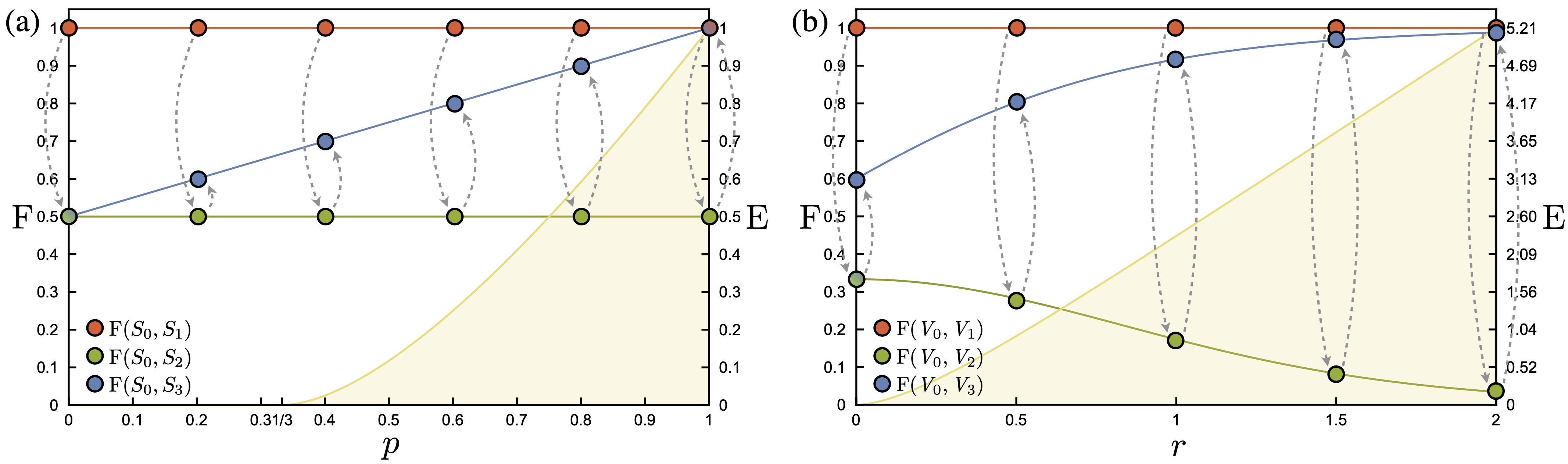
Figure 3: Fidelity of measurement-free teleportation for (a) a 2-dimensional DV system, and (b) a Gaussian CV system for $g_{2}=3$. The value of fidelity, $\mathrm{F}$, is plotted between the input state and the state in the principal system after the operation $\mathit{U}_{1}$ (red line), $\mathit{U}_{2}$ (green line), and $\mathit{U}_{3}$ (blue line). EoF of the resource state, $\mathrm{E}$, is plotted with a yellow line. The resource state in panel (a) is a Werner state parametrized by $p\in[0,1]$, and (b) a two-mode squeezed vacuum parametrized by $r\in[0,2]$. The colored dots show the initial decrease of fidelity after the operation $\mathit{U}_{2}$ and its subsequent increase upon the final operation $\mathit{U}_{3}$. It is apparent that non-Markovianity becomes more pronounced as the entanglement of the resource state increases. In panel (a) a complete state revival (perfect teleportation) is observed for $p=1$, which corresponds to a maximally entangled state, and in panel (b) the the value of fidelity approaches unity as the entanglement of the resource state increases.

In order to examine the relationship between the non-Markovian phenomenon and the entanglement in teleportation, assume that the resource state $\mathit{R}$ is the Werner state $\mathit{W}=p\varPhi+(1-p)\mathds{1}_{4}/4$ [59], where $\mathds{1}_{4}/4$ is the maximally mixed state and $p\in[0,1]$. Note that the Werner state is effectively a Bell state passing through the depolarizing channel. In Fig. 3 (a) we plot the fidelity between an input state $S=S_{0}=\outerproduct{0}{0}$ and the state in the principal system after each operation $\mathit{U}_{i}$ for $i\in\{1,2,3\}$, denoted as $S_{i}$. Fidelity is a way to distinguish two quantum states, defined as $\mathrm{F}(\varPsi_{i},\varPsi_{j})\coloneqq\big{(}\mathrm{tr}\sqrt{\smash[t]{\sqrt{\varPsi_{i}}}\smash[b]{\varPsi_{j}}\smash[b]{\sqrt{\varPsi_{i}}}}\big{)}^{2}$ [60], with $\mathrm{F}(\varPsi_{i},\varPsi_{j})=1\Leftrightarrow\varPsi_{i}=\varPsi_{j}$. We quantify the entanglement of the resource state through entanglement of formation (EoF), denoted as $\mathrm{E}$ [61, 62]. EoF of a state $\varPsi=\sum_{i}p_{i}\outerproduct{\psi_{i}}{\psi_{i}}\in\mathscr{H}^{(\mathrm{A})}{\otimes}\mathscr{H}^{(\mathrm{B})}$ is defined as $\mathrm{E}(\varPsi)\coloneqq\min_{i}\{\sum_{i}p_{i}\mathbb{H}(\mathrm{tr}_{\mathrm{\mathrm{A/B}}}\outerproduct{\psi_{i}}{\psi_{i}})\}$, with $\sum_{i}p_{i}=1$, $\mathbb{H}(\varPsi)\coloneqq-\mathrm{tr}(\varPsi\log_{2}\varPsi)$, and $\mathrm{tr}_{\mathrm{\mathrm{A/B}}}$ denoting the partial trace over either partition A or B. We observe in Fig. 3 (a) a clear relationship between non-Markovianity and the amount of entanglement of the resource state. For a maximally entangled resource state $\mathrm{F}(S_{0},S_{3})$ becomes equal to one, indicating a complete state revival. Note that several quantifiers exist for both non-Markovianity [3, 63] and entanglement [64, 65], and thus any valid measure of them provides qualitatively the same behavior.

V.2 Continuous-variable Teleportation

Measurement-free teleportation in continuous-variable (CV) systems [66] was proposed by Ralph [23] by the name “all-optical teleportation” (see also Ref. [67]) and it was experimentally realized in Ref. [68]. This protocol can be realized through the following non-divisible operation

$$\mathrm{tr}_{\mathrm{E_{2}}}\left\{\mathit{U}_{3}\,\mathrm{tr}_{\mathrm{E_{1}}}[\mathit{U}_{2}\mathit{U}_{1}(S\otimes\mathit{E}_{1}\otimes\mathit{E}_{2})\mathit{U}^{{\dagger}}_{1}\mathit{U}^{{\dagger}}_{2}]\mathit{U}^{{\dagger}}_{3}\right\}=S,$$ (10)

where $S\in\mathscr{H}^{(\mathrm{S})}_{\infty}$ belongs to Alice and $\mathit{E}_{1}{\otimes}\mathit{E}_{2}=\outerproduct{00}{00}\in\mathscr{H}^{(\mathrm{E}_{1})}_{\infty}{\otimes}\mathscr{H}^{(\mathrm{E}_{2})}_{\infty}$ to the environment (similarly to the DV case the term “environment” is used to label the modes that will be traced out after the interaction), as seen in Fig. 2 (b). The unitary operations are given below

$$\mathit{U}_{1} =\mathds{1}_{\infty}\otimes\mathit{Q}[\mathrm{arccosh}\hskip 1.13791pt(\sqrt{g_{1}})],$$ (11a)

$$\mathit{U}_{2} =\mathit{Q}[\mathrm{arccosh}\hskip 1.13791pt(\sqrt{g_{2}})]\otimes\mathds{1}_{\infty},$$ (11b)

$$\mathit{U}_{3} =\mathit{B}(1/{g_{2}}),$$ (11c)

in the limit of $g_{1}\rightarrow\infty$ and $g_{2}\rightarrow\infty$. $\mathit{Q}(r)$ is the two-mode squeezing operation $\mathit{Q}(r)\coloneqq\exp[r(\mathit{A}_{1}\mathit{A}_{2}-\mathit{A}^{{\dagger}}_{1}\mathit{A}^{{\dagger}}_{2})/2]$ with $\mathit{A}$ denoting the annihilation operator and $r\in\mathbbol{R}$ the real-valued squeezing parameter. The subscripts of the operators refer to the mode on which they are applied. The two-mode squeezing operation is the entanglement operation in CV states, i.e., $\mathit{Q}(r)\ket{00}=\sqrt{1-\tanh^{2}r}\sum_{i=0}^{\infty}(-\tanh r)^{i}\ket{ii}$, known as the two-mode squeezed vacuum, which becomes maximally entangled in the limit of $r\rightarrow\infty$. $\mathit{B}(\tau)$ is the beam-splitter operation $\mathit{B}(\tau)\coloneqq\exp[\tau(\mathit{A}_{1}^{{\dagger}}\mathit{A}_{2}-\mathit{A}_{1}\mathit{A}_{2}^{{\dagger}})]$ with $\tau\in[0,1]$ being the transmissivity parameter.

Regarding information flow in this protocol, consider for simplicity a Gaussian CV system [69], where the quantum states can be fully represented through covariance matrices, $\mathit{V}$, and the unitary operations through symplectic transformations, $\varSigma$, i.e., $\mathit{V}\rightarrow\varSigma\mathit{V}\varSigma^{\intercal}$. Let us have the input state $\mathit{V}_{S}=v\,\mathds{1}_{2}$, with $v\geqslant 1$, and two vacuum states for the environment $\mathit{V}_{\mathrm{vac}}\oplus\mathit{V}_{\mathrm{vac}}=\mathds{1}_{2}\oplus\mathds{1}_{2}$, where $\oplus$ denotes the tensor sum when it is applied on matrices. During the first stage, the corresponding symplectic transformation $\varSigma_{1}$ is applied, and the environment becomes maximally entangled,

$$\varSigma_{1}\left(\mathit{V}_{S}\oplus\mathit{V}_{\mathrm{vac}}\oplus\mathit{V}_{\mathrm{vac}}\right)\varSigma_{1}^{\intercal}=\mathit{V}_{S}\oplus\mathit{V}_{\varPhi},$$ (12)

where $\mathit{V}_{\varPhi}$ is the covariance matrix of the state $\lim_{r\rightarrow\infty}\mathit{Q}(r)\ket{00}$. The second stage involves the symplectic transformation $\varSigma_{2}$ and a partial trace over $\mathscr{H}^{(\mathrm{E}_{1})}$, so the covariance matrix transforms into

$$\mathrm{tr}_{\mathrm{E_{1}}}\left[\varSigma_{2}\left(\mathit{V}_{S}\oplus\mathit{V}_{\varPhi}\right)\varSigma_{2}^{\intercal}\right]=\mathrm{tr}_{\mathrm{E_{1}}}\begin{bmatrix}\mathit{V}_{11}&\mathit{V}_{12}&\mathit{V}_{13}\\ \mathit{V}_{21}&\mathit{V}_{22}&\mathit{V}_{23}\\ \mathit{V}_{31}&\mathit{V}_{32}&\mathit{V}_{33}\\ \end{bmatrix},$$ (13)

with submatrices given by $\mathit{V}_{11}=[2g_{1}(g_{2}-1)+g_{2}(v-1)+1]\mathds{1}_{2}$, $\mathit{V}_{22}=[v(g_{2}-1)+g_{2}(2g_{1}-1)]\mathds{1}_{2}$, $\mathit{V}_{33}=(2g_{1}-1)\mathds{1}_{2}$, $\mathit{V}_{12}=\mathit{V}_{21}^{\intercal}=(v+2g_{1}-1)\sqrt{g_{2}(g_{2}-1)}\,\mathit{Z}_{2}$, $\mathit{V}_{13}=\mathit{V}_{31}^{\intercal}=2\sqrt{g_{1}(g_{1}-1)(g_{2}-1)}\,\mathds{1}_{2}$, and $\mathit{V}_{23}=\mathit{V}_{32}^{\intercal}=2\sqrt{g_{1}g_{2}(g_{1}-1)}\,\mathit{Z}_{2}$. Given that prior to the partial trace the matrix in Eq. (13) represents a tri-partite entangled state (see Ref. [70] for appropriate entanglement criteria), information about the input system is transferred in the form of correlations in both modes of environment. Finally, the third symplectic transformation $\varSigma_{3}$ results in a state revival for the principal system,

$$\mathrm{tr}_{\mathrm{E_{2}}}\left\{\varSigma_{3}\mathrm{tr}_{\mathrm{E_{1}}}\left[\varSigma_{2}\left(\mathit{V}_{S}\oplus\mathit{V}_{\varPhi}\right)\varSigma_{2}^{\intercal}\right]\varSigma_{3}^{\intercal}\right\}=\mathit{V}_{S}.$$ (14)

More information about Eqs. (12)-(14) are given in the Supplemental Material.

In order to show how entanglement and non-Markovianity are connected in this protocol, in Fig. 3 (b) we plot the fidelity between an input state $S=S_{0}=\outerproduct{0}{0}$, represented by the covariance matrix $\mathit{V}_{0}=\mathds{1}_{2}$, and the state in the principal system after each operation $\mathit{U}_{i}$ for $i\in\{1,2,3\}$, i.e., $\mathit{V}_{i}$. Fidelity between two single-mode (non-displaced) Gaussian states is defined as $\mathrm{F}(\mathit{V}_{i},\mathit{V}_{j})\coloneqq 2/(\sqrt{\mu+\nu}-\sqrt{\nu})$, where $\mu=\det(\mathit{V}_{i}+\mathit{V}_{j})$ and $\nu=(\det\mathit{V}_{i}-1)(\det\mathit{V}_{j}-1)$ [71, 72]. As a resource state we consider a two-mode squeezed vacuum $\mathit{Q}(r)\ket{00}$ with $r\in[0,2]$, and we quantify its entanglement through EoF, which for this state takes the form $\mathrm{E}(r)=\cosh^{2}r\log_{2}(\cosh^{2}r)-\sinh^{2}r\log_{2}(\sinh^{2}r)$ [73, 74]. Note that the selected range of the squeezing parameter is accessible with current technology, since $r_{\mathrm{max}}=2$ corresponds to $\sim$17.4dB of squeezing. Similarly to the DV case, we observe that non-Markovianity increases as the entanglement of the resource state increases. Since the CV measurement-free teleportation works perfectly in the limit of $r\rightarrow\infty$ and $g_{2}\rightarrow\infty$, $\mathrm{F}(\mathit{V}_{0},\mathit{V}_{3})$ approaches unity but the input state is not completely revived. The use of non-ideal values is also the reason why $\mathrm{F}(\mathit{V}_{0},\mathit{V}_{3})$ for $r=0$ is ${\sim}0.6$ and not 1/2.

VI Conclusion

In this work it is shown that when it is seen from an open quantum system point of view, the protocol of teleportation is a non-Markovian quantum operation, where entanglement provides the means for a complete quantum state revival. This connection is achieved when the teleportation is studied under its measurement-free approach, which is mathematically equivalent to the conventional measurement-based one. In particular, for the continuous-variable case we employ the all-optical teleportation [23], and for the discrete-variable case we extend to finite-dimensional states a measurement-free protocol [22] that was limited to qubits. It is also discussed how the state revival is due to an information back-flow effect given the time-homogeneous nature of the whole process. Teleportation is a fundamental protocol in quantum information [75] that provides a building block for broader applications such as the quantum internet [76, 77, 78] and photonic quantum computers [79, 80, 81]. Thus, the relationship between this protocol and the phenomenon of non-Markovianity creates a new perspective on the information flow during those applications.

VI.1 Acknowledgments

This is supported by the NSF Engineering Research Center (ERC) Center for Quantum Networks and NSF RAISE-QAC-QSA, Grant No. DMR-2037783 on “Open Quantum Systems on Noisy Intermediate-Scale Quantum Devices”. K.H.M. is partially supported by the Department of Energy, Office of Basic Energy Sciences Grant DE-SC0019215 on “Quantum Computing Algorithms and Applications for Coherent and Strongly Correlated Chemical Systems”. P.N. acknowledges support as a Moore Inventor Fellow through Grant No. GBMF8048 and gratefully acknowledges support from the Gordon and Betty Moore Foundation as well as support from a NSF CAREER Award under Grant No. NSF-ECCS-1944085.

supplement.pdf in 1,…,0 See pages \x, of supplement.pdf

References

- Rényi [2007] A. Rényi, Probability Theory (Dover Publications, Mineola, NY, 2007).
- Wolf and Cirac [2008] M. M. Wolf and J. I. Cirac, Dividing quantum channels, Commun. Math. Phys. 279, 147 (2008).
- Rivas et al. [2014] Á. Rivas, S. F. Huelga, and M. B. Plenio, Quantum non-Markovianity: characterization, quantification and detection, Rep. Prog. Phys. 77, 094001 (2014).
- Caruso et al. [2014] F. Caruso, V. Giovannetti, C. Lupo, and S. Mancini, Quantum channels and memory effects, Rev. Mod. Phys. 86, 1203 (2014).
- Breuer et al. [2016] H.-P. Breuer, E.-M. Laine, J. Piilo, and B. Vacchini, Colloquium: Non-Markovian dynamics in open quantum systems, Rev. Mod. Phys. 88, 021002 (2016).
- de Vega and Alonso [2017] I. de Vega and D. Alonso, Dynamics of non-Markovian open quantum systems, Rev. Mod. Phys. 89, 015001 (2017).
- Li et al. [2018] L. Li, M. J. Hall, and H. M. Wiseman, Concepts of quantum non-Markovianity: A hierarchy, Phys. Rep. 759, 1 (2018).
- Milz and Modi [2021] S. Milz and K. Modi, Quantum stochastic processes and quantum non-Markovian phenomena, PRX Quantum 2, 030201 (2021).
- Ciccarello et al. [2022] F. Ciccarello, S. Lorenzo, V. Giovannetti, and G. M. Palma, Quantum collision models: Open system dynamics from repeated interactions, Phys. Rep. 954, 1 (2022).
- Breuer et al. [2009] H.-P. Breuer, E.-M. Laine, and J. Piilo, Measure for the degree of non-Markovian behavior of quantum processes in open systems, Phys. Rev. Lett. 103, 210401 (2009).
- Piilo et al. [2009] J. Piilo, K. Härkönen, S. Maniscalco, and K.-A. Suominen, Open system dynamics with non-markovian quantum jumps, Phys. Rev. A 79, 062112 (2009).
- Laine et al. [2010] E.-M. Laine, J. Piilo, and H.-P. Breuer, Measure for the non-Markovianity of quantum processes, Phys. Rev. A 81, 062115 (2010).
- Lo Franco et al. [2012] R. Lo Franco, B. Bellomo, E. Andersson, and G. Compagno, Revival of quantum correlations without system-environment back-action, Phys. Rev. A 85, 032318 (2012).
- Chruściński and Wudarski [2013] D. Chruściński and F. A. Wudarski, Non-Markovian random unitary qubit dynamics, Phys. Lett. A 377, 1425 (2013).
- Megier et al. [2017] N. Megier, D. Chruściński, J. Piilo, and W. T. Strunz, Eternal non-Markovianity: from random unitary to markov chain realisations, Sci. Rep. 7, 6379 (2017).
- Chruściński and Maniscalco [2014] D. Chruściński and S. Maniscalco, Degree of non-Markovianity of quantum evolution, Phys. Rev. Lett. 112, 120404 (2014).
- Budini [2018] A. A. Budini, Maximally non-Markovian quantum dynamics without environment-to-system backflow of information, Phys. Rev. A 97, 052133 (2018).
- Bennett et al. [1993] C. H. Bennett, G. Brassard, C. Crépeau, R. Jozsa, A. Peres, and W. K. Wootters, Teleporting an unknown quantum state via dual classical and einstein-podolsky-rosen channels, Phys. Rev. Lett. 70, 1895 (1993).
- Braunstein and Kimble [1998] S. L. Braunstein and H. J. Kimble, Teleportation of continuous quantum variables, Phys. Rev. Lett. 80, 869 (1998).
- Deutsch and Hayden [2000] D. Deutsch and P. Hayden, Information flow in entangled quantum systems, Proc. R. Soc. Lond. A. 456, 1759 (2000).
- Horodecki et al. [2001] R. Horodecki, M. Horodecki, and P. Horodecki, Balance of information in bipartite quantum-communication systems: Entanglement-energy analogy, Phys. Rev. A 63, 022310 (2001).
- Brassard et al. [1998] G. Brassard, S. L. Braunstein, and R. Cleve, Teleportation as a quantum computation, Physica D 120, 43 (1998).
- Ralph [1999] T. C. Ralph, All-optical quantum teleportation, Opt. Lett. 24, 348 (1999).
- Rivas et al. [2010] A. Rivas, S. F. Huelga, and M. B. Plenio, Entanglement and non-Markovianity of quantum evolutions, Phys. Rev. Lett. 105, 050403 (2010).
- Vasile et al. [2010] R. Vasile, P. Giorda, S. Olivares, M. G. A. Paris, and S. Maniscalco, Nonclassical correlations in non-Markovian continuous-variable systems, Phys. Rev. A 82, 012313 (2010).
- Maniscalco et al. [2007] S. Maniscalco, S. Olivares, and M. G. A. Paris, Entanglement oscillations in non-Markovian quantum channels, Phys. Rev. A 75, 062119 (2007).
- Reina et al. [2014] J. H. Reina, C. E. Susa, and F. F. Fanchini, Entanglement revive and information flow within the decoherent environment, Sci. Rep. 4, 1 (2014).
- Shi et al. [2016] J.-d. Shi, D. Wang, and L. Ye, Entanglement revive and information flow within the decoherent environment, Sci. Rep. 6, 30710 (2016).
- Mirkin et al. [2019a] N. Mirkin, P. Poggi, and D. Wisniacki, Entangling protocols due to non-Markovian dynamics, Phys. Rev. A 99, 020301(R) (2019a).
- Mirkin et al. [2019b] N. Mirkin, P. Poggi, and D. Wisniacki, Information backflow as a resource for entanglement, Phys. Rev. A 99, 062327 (2019b).
- Li et al. [2021] X.-M. Li, Y.-X. Chen, Y.-J. Xia, and Z.-X. Man, Effect of entanglement embedded in environment on quantum non-Markovianity based on collision model, Commun. Theor. Phys. 73, 055104 (2021).
- Breuer and Petruccione [2002] H.-P. Breuer and F. Petruccione, The Theory of Open Quantum Systems (Oxford University Press, New York, NY, 2002).
- Nielsen and Chuang [2010] M. A. Nielsen and I. L. Chuang, Quantum Computation and Quantum Information, 1st ed. (Cambridge University Press, New York, NY, 2010).
- Stinespring [1955] W. F. Stinespring, Positive functions on C∗-algebras, Proc. Am. Math. Soc. 6, 211 (1955).
- Sudarshan et al. [1961] E. C. G. Sudarshan, P. M. Mathews, and J. Rau, Stochastic dynamics of quantum-mechanical systems, Phys. Rev. 121, 920 (1961).
- Hellwig and Kraus [1970] K. E. Hellwig and K. Kraus, Operations and measurements. II, Comm. Math. Phys. 16, 142 (1970).
- Mendl and Wolf [2009] C. B. Mendl and M. M. Wolf, Unital quantum channels – convex structure and revivals of birkhoff’s theorem, Commun. Math. Phys. 289, 1057 (2009).
- Watrous [2018] J. Watrous, The Theory of Quantum Information, 1st ed. (Cambridge University Press, New York, NY, 2018).
- Liu et al. [2011] B.-H. Liu, L. Li, Y.-F. Huang, C.-F. Li, G.-C. Guo, E.-M. Laine, H.-P. Breuer, and J. Piilo, Experimental control of the transition from Markovian to non-Markovian dynamics of open quantum systems, Nat. Physics 7, 931 (2011).
- Chiuri et al. [2012] A. Chiuri, C. Greganti, L. Mazzola, M. Paternostro, and P. Mataloni, Linear optics simulation of quantum non-markovian dynamics, Sci. Rep. 2, 968 (2012).
- Liu et al. [2013] B.-H. Liu, D.-Y. Cao, Y.-F. Huang, C.-F. Li, G.-C. Guo, E.-M. Laine, H.-P. Breuer, and J. Piilo, Photonic realization of nonlocal memory effects and non-Markovian quantum probes, Sci. Rep. 3, 1781 (2013).
- Cialdi et al. [2017] S. Cialdi, M. A. C. Rossi, C. Benedetti, B. Vacchini, D. Tamascelli, S. Olivares, and M. G. A. Paris, All-optical quantum simulator of qubit noisy channels, Appl. Phys. Lett. 110, 081107 (2017).
- Liu et al. [2018] Z.-D. Liu, H. Lyyra, Y.-N. Sun, B.-H. Liu, C.-F. Li, G.-C. Guo, S. Maniscalco, and J. Piilo, Experimental implementation of fully controlled dephasing dynamics and synthetic spectral densities, Nat. Commun. 9, 3453 (2018).
- Cuevas et al. [2019] Á. Cuevas, A. Geraldi, C. Liorni, L. D. Bonavena, A. D. Pasquale, F. Sciarrino, V. Giovannetti, and P. Mataloni, All-optical implementation of collision-based evolutions of open quantum systems, Sci. Rep. 9, 3205 (2019).
- Wittemer et al. [2018] M. Wittemer, G. Clos, H.-P. Breuer, U. Warring, and T. Schaetz, Measurement of quantum memory effects and its fundamental limitations, Phys. Rev. A 97, 020102(R) (2018).
- Bernardes et al. [2016] N. K. Bernardes, J. P. S. Peterson, R. S. Sarthour, A. M. Souza, C. H. Monken, I. Roditi, I. S. Oliveira, and M. F. Santos, High resolution non-markovianity in NMR, Sci. Rep. 6, 33945 (2016).
- Sweke et al. [2016] R. Sweke, M. Sanz, I. Sinayskiy, F. Petruccione, and E. Solano, Digital quantum simulation of many-body non-Markovian dynamics, Phys. Rev. A 94, 022317 (2016).
- García-Pérez et al. [2020] G. García-Pérez, M. A. C. Rossi, and S. Maniscalco, IBM q experience as a versatile experimental testbed for simulating open quantum systems, Npj Quantum Inf. 6, 1 (2020).
- Hu et al. [2020] Z. Hu, R. Xia, and S. Kais, A quantum algorithm for evolving open quantum dynamics on quantum computing devices, Sci. Rep. 10, 3301 (2020).
- Head-Marsden et al. [2021] K. Head-Marsden, S. Krastanov, D. A. Mazziotti, and P. Narang, Capturing non-Markovian dynamics on near-term quantum computers, Phys. Rev. Research 3, 013182 (2021).
- Buscemi and Datta [2016] F. Buscemi and N. Datta, Equivalence between divisibility and monotonic decrease of information in classical and quantum stochastic processes, Phys. Rev. A 93, 012101 (2016).
- Horodecki and Horodecki [1998] M. Horodecki and R. Horodecki, Are there basic laws of quantum information processing?, Phys. Lett. A 244, 473 (1998).
- Nielsen et al. [1998] M. A. Nielsen, E. Knill, and R. Laflamme, Complete quantum teleportation using nuclear magnetic resonance, Nature 396, 52 (1998).
- Garcia-Escartin and Chamorro-Posada [2013] J. C. Garcia-Escartin and P. Chamorro-Posada, A SWAP gate for qudits, Quantum Inf. Process. 12, 3625 (2013).
- Wang et al. [2020] Y. Wang, Z. Hu, B. C. Sanders, and S. Kais, Qudits and high-dimensional quantum computing, Front. Phys. 8, 479 (2020).
- Alber et al. [2001] G. Alber, A. Delgado, N. Gisin, and I. Jex, Efficient bipartite quantum state purification in arbitrary dimensional Hilbert spaces, J. of Phys. A: Math. Gen. 34, 8821 (2001).
- Braunstein [1996] S. L. Braunstein, Quantum teleportation without irreversible detection, Phys. Rev. A 53, 1900 (1996).
- Roa et al. [2003] L. Roa, A. Delgado, and I. Fuentes-Guridi, Optimal conclusive teleportation of quantum states, Phys. Rev. A 68, 022310 (2003).
- Werner [1989] R. F. Werner, Quantum states with Einstein-Podolsky-Rosen correlations admitting a hidden-variable model, Phys. Rev. A 40, 4277 (1989).
- Jozsa [1994] R. Jozsa, Fidelity for mixed quantum states, J. Mod. Opt. 41, 2315 (1994).
- Bennett et al. [1996] C. H. Bennett, D. P. DiVincenzo, J. A. Smolin, and W. K. Wootters, Mixed-state entanglement and quantum error correction, Phys. Rev. A 54, 3824 (1996).
- Wootters [1998] W. K. Wootters, Entanglement of formation of an arbitrary state of two qubits, Phys. Rev. Lett. 80, 2245 (1998).
- Addis et al. [2014] C. Addis, B. Bylicka, D. Chruściński, and S. Maniscalco, Comparative study of non-Markovianity measures in exactly solvable one- and two-qubit models, Phys. Rev. A 90, 052103 (2014).
- Horodecki et al. [2009] R. Horodecki, P. Horodecki, M. Horodecki, and K. Horodecki, Quantum entanglement, Rev. Mod. Phys. 81, 865 (2009).
- Plenio and Virmani [2014] M. B. Plenio and S. S. Virmani, An introduction to entanglement theory, in Quantum Information and Coherence, edited by E. Andersson (Springer International Publishing, Cham, 2014) pp. 173–209.
- Serafini [2017] A. Serafini, Quantum Continuous Variables: A Primer of Theoretical Methods, 1st ed. (CRC Press, Boca Raton, FL, 2017).
- Tserkis et al. [2020] S. Tserkis, N. Hosseinidehaj, N. Walk, and T. C. Ralph, Teleportation-based collective attacks in Gaussian quantum key distribution, Phys. Rev. Research 2, 013208 (2020).
- Liu et al. [2020] S. Liu, Y. Lou, and J. Jing, Orbital angular momentum multiplexed deterministic all-optical quantum teleportation, Nat. Commun. 11, 3875 (2020).
- Weedbrook et al. [2012] C. Weedbrook, S. Pirandola, R. García-Patrón, N. J. Cerf, T. C. Ralph, J. H. Shapiro, and S. Lloyd, Gaussian quantum information, Rev. Mod. Phys. 84, 621 (2012).
- Teh and Reid [2014] R. Y. Teh and M. D. Reid, Criteria for genuine -partite continuous-variable entanglement and Einstein-Podolsky-Rosen steering, Phys. Rev. A 90, 062337 (2014).
- Nha and Carmichael [2005] H. Nha and H. J. Carmichael, Distinguishing two single-mode Gaussian states by homodyne detection: An information-theoretic approach, Phys. Rev. A 71, 032336 (2005).
- Banchi et al. [2015] L. Banchi, S. L. Braunstein, and S. Pirandola, Quantum fidelity for arbitrary Gaussian states, Phys. Rev. Lett. 115, 260501 (2015).
- Giedke et al. [2003] G. Giedke, M. M. Wolf, O. Krüger, R. F. Werner, and J. I. Cirac, Entanglement of formation for symmetric Gaussian states, Phys. Rev. Lett. 91, 107901 (2003).
- Tserkis and Ralph [2017] S. Tserkis and T. C. Ralph, Quantifying entanglement in two-mode Gaussian states, Phys. Rev. A 96, 062338 (2017).
- Pirandola et al. [2015] S. Pirandola, J. Eisert, C. Weedbrook, A. Furusawa, and S. L. Braunstein, Advances in quantum teleportation, Nat. Photonics 9, 641 (2015).
- Kimble [2008] H. J. Kimble, The quantum internet, Nature 453, 1023 (2008).
- Perseguers et al. [2013] S. Perseguers, G. J. Lapeyre, D. Cavalcanti, M. Lewenstein, and A. Acín, Distribution of entanglement in large-scale quantum networks, Rep. Prog. Phys. 76, 096001 (2013).
- Wehner et al. [2018] S. Wehner, D. Elkouss, and R. Hanson, Quantum internet: A vision for the road ahead, Science 362, 303 (2018).
- Kok et al. [2007] P. Kok, W. J. Munro, K. Nemoto, T. C. Ralph, J. P. Dowling, and G. J. Milburn, Linear optical quantum computing with photonic qubits, Rev. Mod. Phys. 79, 135 (2007).
- Bourassa et al. [2021] J. E. Bourassa, R. N. Alexander, M. Vasmer, A. Patil, I. Tzitrin, T. Matsuura, D. Su, B. Q. Baragiola, S. Guha, G. Dauphinais, K. K. Sabapathy, N. C. Menicucci, and I. Dhand, Blueprint for a Scalable Photonic Fault-Tolerant Quantum Computer, Quantum 5, 392 (2021).
- Bartolucci et al. [2021] S. Bartolucci, P. Birchall, H. Bombin, H. Cable, C. Dawson, M. Gimeno-Segovia, E. Johnston, K. Kieling, N. Nickerson, M. Pant, F. Pastawski, T. Rudolph, and C. Sparrow, Fusion-based quantum computation, arXiv:2101.09310 (2021).
supplement.pdf \foreach\xin 1,…,0 See pages \x, of supplement.pdf