Parsing Randomness

Abstract.

“A generator is a parser of randomness.” This perspective on generators for random data structures is well established as folklore in the programming languages community, but it has apparently never been formalized, nor have its consequences been deeply explored.

We present free generators, which unify parsing and generation using a common structure that makes the relationship between the two concepts precise. Free generators lead naturally to a proof that a large class of generators can be factored into a parser plus a distribution over choice sequences. Further, free generators support a notion of derivative, analogous to familiar Brzozowski derivatives of formal languages, that allows analysis tools to “preview” the effect of a particular generator choice. This, in turn, gives rise to a novel algorithm for generating data structures satisfying user-specified preconditions.

1. Introduction

“A generator is a parser of randomness…” It’s one of those observations that’s totally puzzling right up to the moment it becomes totally obvious: a random generator—such as might be found in a property-based testing tool like QuickCheck (Claessen and Hughes, 2000)—is a transformer from a series of random choices into a data structure, just as a parser transforms a series of characters into a data structure.

Although this connection may be obvious once it is pointed out, few actually think of generators this way. Indeed, to our knowledge the framing of random generators as parsers has never been explored formally. But this is a shame! The relationship between these fundamental concepts deserves a deeper look.

A generator is a program that builds a data structure by making a sequence of random choices—those choices are the key. A “traditional” generator makes decisions using a stored source of randomness (e.g., a seed) that it consults and updates whenever it must make a choice. Equivalently, if we like, we can pre-compute a list of choices and pass it in to the generator, which gradually walks down the list whenever it needs to make random decisions. In this mode of operation, the generator is effectively parsing the sequence of choices into a data structure!

To connect generators and parsers, we introduce a data structure called a free generator that can be interpreted as either a generator or as a parser. Free generators have a rich theory; in particular, we can use them to prove that a subset of generator programs can be factored into a parser and a distribution over sequences of choices.

Besides clarifying folklore, free generators admit transformations that cannot be implemented for standard generators and parsers. A particularly exciting one is a notion of derivative which modifies a generator by asking the question: “what would this generator look like after it makes choice $c$?” The derivative gives a way of previewing a particular choice to determine how likely it is to lead us to useful values.

We use derivatives of free generators to tackle a well-known problem—we call it the valid generation problem. The challenge is to generate a large number of random values that satisfy some validity condition. This problem comes up often in property-based testing, where the validity condition is the precondition of some functional specification. Since generator derivatives give a way of previewing the effects of a particular choice, we can use gradients (derivatives with respect to a vector of choices) to preview all possible choices and pick a promising one. This leads us to an elegant algorithm for turning a naïve free generator into one that only generates valid values.

In §2 below, we introduce the ideas behind free generators and the operations that can be defined on them. We then present our main contributions:

• We formalize the folklore analogy between parsers and generators using free generators, a novel class of structures that make choices explicit and support syntactic transformations (§3). We use free generators to prove that every “applicative” generator can factored into a parser and a probability distribution.

• We exploit free generators to to transport an idea from formal languages—the Brzozowski derivative—to the context of generators (§4).

• To illustrate the potential applications of these formal results, we present an algorithm that uses derivatives to turn a naïve generator into one that produces only values satisfying a Boolean precondition (§5). Our algorithm performs well on simple benchmarks, in most cases producing more than twice as many valid values as a naïve “rejection sampling” generator in the same amount of time (§6).

We conclude with related and future work (§7 and §8).

2. The High-Level Story

Let’s take a walk in the forest before we dissect the trees.

Generators and Parsers. Consider the generator genTree in Figure 1, which produces random binary trees of Booleans like

Node True Leaf Leaf  and

Node True Leaf (Node False Leaf Leaf),

up to a given height $h$, guided by a series of random coin flips.

genTree $h$ =

     if $h=0$ then

         return Leaf

     else

         $c\leftarrow\textsf{flip}()$

         if $c==\textsf{Heads}$ then return Leaf          

         if $c==\textsf{Tails}$ then

              $c\leftarrow\textsf{flip}()$

              if $c==\textsf{Heads}$ then $x\leftarrow\textsf{True}$               

              if $c==\textsf{Tails}$ then $x\leftarrow\textsf{False}$               

              $l\leftarrow\textsf{genTree}~{}(h-1)$

              $r\leftarrow\textsf{genTree}~{}(h-1)$

              $\textbf{return}~{}\textsf{Node}~{}x~{}l~{}r$                

parseTree $h$ =

     if $h=0$ then

         return Leaf

     else

         $c\leftarrow\textsf{consume}()$

         if $c=={\color[rgb]{0.0078125,0.46875,0.17578125}\tt l}$ then return Leaf          

         if $c=={\color[rgb]{0.0078125,0.46875,0.17578125}\tt n}$ then

              $c\leftarrow\textsf{consume}()$

              if $c=={\color[rgb]{0.0078125,0.46875,0.17578125}\tt t}$ then $x\leftarrow\textsf{True}$               

              if $c=={\color[rgb]{0.0078125,0.46875,0.17578125}\tt f}$ then $x\leftarrow\textsf{False}$

              else fail               

              $l\leftarrow\textsf{parseTree}~{}(h-1)$

              $r\leftarrow\textsf{parseTree}~{}(h-1)$

              $\textbf{return}~{}\textsf{Node}~{}x~{}l~{}r$

         else fail                

Figure 1. A generator and a parser for Boolean binary trees.

Now, consider parseTree (also in Figure 1), which parses a string over the characters n, l, t, and f into a tree. The parser turns

ntll into Node True Leaf Leaf  and

ntlnfll into Node True Leaf (Node False Leaf Leaf).

It consumes the input string character by character with consume and uses the characters to decide what to do next.

Obviously, there is considerable structural similarity between genTree and parseTree. One apparent difference lies in the way they make choices and the “labels” for those choices: in genTree, choices are made randomly during the execution of the program and are marked by sides of a coin, while in parseTree the choices are made ahead of time and manifest as the characters in the input string. But this difference is rather superficial.

Free Generators. We can unify random generation with parsing by abstracting both into a single data structure. For this, we introduce [free generator]free generators. Free generators are syntactic structures (a bit like abstract syntax trees) that can be interpreted as programs that either generate or parse. Observe the structural similarities between fgenTree and the programs in Figure 1.

fgenTree $h$ =

     if $h=0$ then

         Pure Leaf

     else

⬇

Select

[ (${\color[rgb]{0.0078125,0.46875,0.17578125}\tt l}$, Pure Leaf),

(${\color[rgb]{0.0078125,0.46875,0.17578125}\tt n}$, MapR

(Pair (Select

[ (${\color[rgb]{0.0078125,0.46875,0.17578125}\tt t}$, Pure True),

(${\color[rgb]{0.0078125,0.46875,0.17578125}\tt f}$, Pure False) ])

(Pair (fgenTree ($h$ - 1))

(fgenTree ($h$ - 1))))

(\ (x, (l, r)) $\rightarrow$ Node x l r)) ]

     

Figure 2. A free generator for binary trees of Booleans.

While the free generator fgenTree $h$ is just a data structure, its shape is much the same as genTree and parseTree. A Pure node in the free generator corresponds roughly to return; it represents a pure value that makes no choices. MapR takes two arguments, a free generator and a function that will eventually be applied to the result of generation / parsing. The Pair constructor maps to sequencing the original programs: it generates / parses using its first argument, then does the same with its second argument, and finally pairs the results together. Finally—the real magic—lies in how we interpret the Select structure. When we want a generator, we treat it as making a uniform random choice, and when we want a parser we treat it as consuming a character $c$ and checking it against the first elements of the pairs.

In §3 we give formal definitions of free generators, along with several interpretation functions. We write $\kl[generatorinterpretation]{\mathcal{G}}\llbracket{}\cdot\rrbracket{}$ for the generator interpretation of a free generator and $\kl[parserinterpretation]{\mathcal{P}}\llbracket{}\cdot\rrbracket{}$ for the parser interpretation. In other words,

$\kl[generatorinterpretation]{\mathcal{G}}\llbracket{}\textsf{fgenTree}~{}5\rrbracket{}~{}\approx~{}\textsf{genTree}~{}5$  and $\kl[parserinterpretation]{\mathcal{P}}\llbracket{}\textsf{fgenTree}~{}5\rrbracket{}~{}\approx~{}\textsf{parseTree}~{}5$.

Now let’s consider how the generator and parser interpretations relate. The key lies in one final interpretation function, $\kl[choicedistribution]{\mathcal{C}}\llbracket{}\cdot\rrbracket{}$, which yields the choice distribution. Intuitively, the choice distribution interpretation produces the set of sequences of choices that the generator interpretation can make, or equivalently the set of sequences that the parser interpretation can parse.

The choice distribution interpretation is used below in Theorem 3.4 to connect parsing and generation. The theorem says that for any free generator $g$,

$$\kl[parserinterpretation]{\mathcal{P}}\llbracket{}g\rrbracket{}\operatorname{\kl[functor]{\langle{}\${}\rangle{}}}\kl[choicedistribution]{\mathcal{C}}\llbracket{}g\rrbracket{}\approx\kl[generatorinterpretation]{\mathcal{G}}\llbracket{}g\rrbracket{}$$

where $\operatorname{\kl[functor]{\langle{}\${}\rangle{}}}$ is a “mapping” operation that applies a function to samples from a distribution. Since many normal QuickCheck generators can also be written as free generators, another way to read this theorem is that such generators can be factored into two pieces: a distribution over choice sequences (given by $\kl[choicedistribution]{\mathcal{C}}\llbracket{}\cdot\rrbracket{}$), and a parser of those sequences (given by $\kl[parserinterpretation]{\mathcal{P}}\llbracket{}\cdot\rrbracket{}$). This precisely formalizes the intuition that “A generator is a parser of randomness.”

Derivatives of Free Generators. But wait, there’s more! Since a free generator defines a parser, it also defines a formal language: we write $\kl[languageofafreegenerator]{\mathcal{L}}\llbracket{}\cdot\rrbracket{}$ for this language interpretation of a free generator. The language of a free generator is the set of choice sequences that it can parse (or make).

Viewing free generators this way suggests some interesting ways that free generators might be manipulated. In particular, formal languages come with a notion of derivative, due to Brzozowski (Brzozowski, 1964). Given a language $L$, the Brzozowski derivative of $L$ is

$$\delta_{c}L=\{s\mid c\cdot s\in L\}.$$

That is, the derivative of $L$ with respect to $c$ is all the strings in $L$ that start with $c$, with the first $c$ removed.

Conceptually, the derivative of a parser with respect to a character $c$ is whatever parser remains after $c$ has just been parsed. For example, the derivative of parseTree 5 with respect to n is:

$\delta_{{\color[rgb]{0.0078125,0.46875,0.17578125}\tt n}}$(parseTree 5) $\approx$      $c\leftarrow\textsf{consume}()$      if $c=={\color[rgb]{0.0078125,0.46875,0.17578125}\tt t}$ then $x\leftarrow\textsf{True}$            if $c=={\color[rgb]{0.0078125,0.46875,0.17578125}\tt f}$ then $x\leftarrow\textsf{False}$      else fail            $l\leftarrow\textsf{parseTree}~{}4$      $r\leftarrow\textsf{parseTree}~{}4$      $\textbf{return}~{}\textsf{Node}~{}x~{}l~{}r$ After parsing the character n, the next step in the original parser is to parse either t or f and then construct a Node; the derivative does just that.

Next let’s take a derivative of the new parser $\delta_{{\color[rgb]{0.0078125,0.46875,0.17578125}\tt n}}(\textsf{parseTree}~{}5)$—this time with respect to t:

$\delta_{{\color[rgb]{0.0078125,0.46875,0.17578125}\tt t}}\delta_{{\color[rgb]{0.0078125,0.46875,0.17578125}\tt n}}$(parseTree 5) $\approx$      $l\leftarrow\textsf{parseTree}~{}4$      $r\leftarrow\textsf{parseTree}~{}4$      $\textbf{return}~{}\textsf{Node}~{}\textsf{True}~{}l~{}r$ Now we have fixed the value True for $x$, and we can continue by making the recursive calls to parseTree 4 and constructing the final tree.

Free generators have a closely related notion of (GEN)derivative. The derivatives of the free generator produced by fgenTree look almost identical to the ones that we saw above for parseTree:

$\kl[generatorderivative]{\delta}_{{\color[rgb]{0.0078125,0.46875,0.17578125}\tt n}}$(fgenTree 5) $\approx$ ⬇ MapR (Pair (Select [ (${\color[rgb]{0.0078125,0.46875,0.17578125}\tt t}$, Pure True), (${\color[rgb]{0.0078125,0.46875,0.17578125}\tt f}$, Pure False) ]) (Pair (fgenTree 4) (fgenTree 4))) (\ (x, (l, r)) $\rightarrow$ Node x l r)

$\kl[generatorderivative]{\delta}_{{\color[rgb]{0.0078125,0.46875,0.17578125}\tt t}}\kl[generatorderivative]{\delta}_{{\color[rgb]{0.0078125,0.46875,0.17578125}\tt n}}$(fgenTree 5) $\approx$

⬇

MapR

(Pair (fgenTree 4)

(fgenTree 4))

(\ (l, r) $\rightarrow$ Node True l r)

Moreover, like derivatives of regular expressions and context-free grammars, derivatives of free generators can be computed by a simple syntactic transformation. In §4 we define a procedure for computing the derivative of a free generator and prove it correct, in the sense that, for all free generators $g$,

$$\delta_{c}\kl[languageofafreegenerator]{\mathcal{L}}\llbracket{}g\rrbracket{}=\kl[languageofafreegenerator]{\mathcal{L}}\llbracket{}\kl[generatorderivative]{\delta}_{c}g\rrbracket{}.$$

In other words, the derivative of the language of $g$ is equal to the language of the derivative of $g$. (See Theorem 4.2.)

Putting Free Generators to Work. The derivative of a free generator is intuitively the generator that remains after a particular choice. This gives us a way of “previewing” the effect of making a choice by looking at the generator after fixing that choice.

In §5 and §6 we present and evaluate an algorithm called [cgs]Choice Gradient Sampling that uses free generators to address the valid generation problem. Given a validity predicate on a data structure, the goal is to generate as many unique, valid structures as possible in a given amount of time. Given a simple free generator, our algorithm uses derivatives to evaluate choices and search for valid values.

We evaluate our algorithm on four small benchmarks, all standard in the property-based testing literature. We compare our algorithm to rejection sampling—sampling from a naïve generator and discarding invalid results—as a simple but useful baseline for understanding how well or algorithm performs. Our algorithm does remarkably well on all but one benchmark, generating more than twice as many valid values as rejection sampling in the same period of time.

3. Free Generators

We now turn to developing the theory of free generators, beginning with some background on applicative abstractions for parsing and random generation.

Background: Applicative Parsers and Generators. In §2 we represented generators and parsers with pseudo-code. Here we flesh out the details. We present all definitions as Haskell programs, both for the sake of concreteness and also because Haskell’s abstraction features (e.g., typeclasses) allow us to focus on the key concepts. Haskell is a lazy functional language, but our results are also applicable to eager functional languages and imperative languages.

We represent both generators and parsers using applicative functors (McBride and Paterson, 2008) At a high level, an applicative functor is a type constructor f with operations:

⬇

($\operatorname{\kl[functor]{\langle{}\${}\rangle{}}}$) :: (a $\rightarrow$ b) $\rightarrow$ f a $\rightarrow$ f b

[applicative]pure :: a $\rightarrow$ f a

([applicative]$\langle*\rangle$) :: f (a $\rightarrow$ b) $\rightarrow$ f a $\rightarrow$ f b

When it might not be clear which applicative functor we mean, we prefix the operator with the name of the functor (e.g., Gen.$\operatorname{\kl[functor]{\langle{}\${}\rangle{}}}$). These operations are mainly useful as a way to apply functions to values inside of some data structure or computation. For example, the idiom “g $\operatorname{\kl[functor]{\langle{}\${}\rangle{}}}$ x [applicative]$\langle*\rangle$ y [applicative]$\langle*\rangle$ z” applies a pure function g to the values in three structures x, y, and z.

We can use these operations to define genTree like we would in QuickCheck (Claessen and Hughes, 2000), since the QuickCheck type constructor Gen, which represents generators, is an applicative functor:
⬇ genTree :: Int $\rightarrow$ Gen Tree genTree 0 = [applicative]pure Leaf genTree $h$ = oneof [ [applicative]pure Leaf, Node $\operatorname{\kl[functor]{\langle{}\${}\rangle{}}}$ genInt [applicative]$\langle*\rangle$ genTree ($h$ - 1) [applicative]$\langle*\rangle$ genTree ($h$ - 1) ] Here, pure is the trivial generator that always generates the same value, and Node $\operatorname{\kl[functor]{\langle{}\${}\rangle{}}}$ g1 [applicative]$\langle*\rangle$ g2 [applicative]$\langle*\rangle$ g3 means apply the constructor Node to three sub-generators to produce a new generator. Operationally, this means sampling x1 from g1, x2 from g2, and x3 from g3, and then constructing Node x1 x2 x3. Notice that we need one extra function beyond the applicative interface: oneof makes a uniform choice between generators, just as we saw in the pseudo-code.

We can do the same thing for parseTree, using combinators inspired by libraries like Parsec (Leijen and Meijer, 2001):
⬇ parseTree :: Int $\rightarrow$ Parser Tree parseTree 0 = [applicative]pure Leaf parseTree $h$ = choice [ (${\color[rgb]{0.0078125,0.46875,0.17578125}\tt l}$, [applicative]pure Leaf), (${\color[rgb]{0.0078125,0.46875,0.17578125}\tt n}$, Node $\operatorname{\kl[functor]{\langle{}\${}\rangle{}}}$ parseInt [applicative]$\langle*\rangle$ parseTree ($h$ - 1) [applicative]$\langle*\rangle$ parseTree ($h$ - 1)) ] In this context, [applicative]pure is a parser that consumes no characters and never fails. It just produces the value passed to it. We can interpret Node $\operatorname{\kl[functor]{\langle{}\${}\rangle{}}}$ p1 [applicative]$\langle*\rangle$ p2 [applicative]$\langle*\rangle$ p3 as running each sub-parser in sequence (failing if any of them fail) and then wrapping the results in the Node constructor. Finally, we have replaced oneof with choice, but the idea is the same: choose between sub-parsers.

Parsers like this have type String $\rightarrow$ Maybe (a, String). They can be applied to a string to obtain either Nothing or Just (a, s), where a is the parse result and s contains any extra characters.

Representing Free Generators. With the applicative interface in mind, we can now give the formal definition of a free generator.

Type Definition. We represent free generators as an inductive data type, FGen, defined as:
⬇ data FGen a where Void :: FGen a Pure :: a $\rightarrow$ FGen a Pair :: FGen a $\rightarrow$ FGen b $\rightarrow$ FGen (a, b) Map :: (a $\rightarrow$ b) $\rightarrow$ FGen a $\rightarrow$ FGen b Select :: List (Char, FGen a) $\rightarrow$ FGen a These constructors form an abstract syntax tree with nodes that roughly correspond to the functions in the applicative interface. Clearly Pure represents pure. Pair is a slightly different form of [applicative]$\langle*\rangle$; one is definable from the other, but this version makes more sense as a data constructor. Map corresponds to $\operatorname{\kl[functor]{\langle{}\${}\rangle{}}}$ (but note that the arguments to Map are flipped relative to MapR from §2). Finally, Select subsumes both oneof and choice: it might mean either, depending on the interpretation. Finally Void represents an always-failing parser or a generator of nothing.

Free generators draw inspiration from free applicative functors (Capriotti and Kaposi, 2014). As with free applicative functors, we can write transformations FGen a $\rightarrow$ f a for any f with similar structure. This fact motivates the rest of this section.

Language of a Free Generator. The language of a free generator is the set of choice sequences that it can make or parse. It is defined recursively, by cases:
⬇ $\kl[languageofafreegenerator]{\mathcal{L}}$$\llbracket$$\cdot$$\rrbracket$ :: FGen a $\rightarrow$ Set String $\kl[languageofafreegenerator]{\mathcal{L}}$$\llbracket$Void$\rrbracket$ = $\varnothing$ $\kl[languageofafreegenerator]{\mathcal{L}}$$\llbracket$Pure a$\rrbracket$ = $\varepsilon$ $\kl[languageofafreegenerator]{\mathcal{L}}$$\llbracket$Map f x$\rrbracket$ = $\kl[languageofafreegenerator]{\mathcal{L}}$$\llbracket$x$\rrbracket$ $\kl[languageofafreegenerator]{\mathcal{L}}$$\llbracket$Pair x y$\rrbracket$ = {s $\cdot$ t | s $\in$ $\kl[languageofafreegenerator]{\mathcal{L}}$$\llbracket$x$\rrbracket$ $\wedge$ t $\in$ $\kl[languageofafreegenerator]{\mathcal{L}}$$\llbracket$y$\rrbracket$} $\kl[languageofafreegenerator]{\mathcal{L}}$$\llbracket$Select xs$\rrbracket$ = {c $\cdot$ s | (c, x) $\in$ xs $\wedge$ s $\in$ $\kl[languageofafreegenerator]{\mathcal{L}}$$\llbracket$x$\rrbracket$}

Smart Constructors and Simplified Forms. Free generators admit a useful simplified form. To ensure that generators are simplified, we can require that free generators be built using smart constructors.

In particular, instead of using Pair directly, we can pair free generators with the smart constructor $\otimes$
⬇ ($\otimes$) :: FGen a $\rightarrow$ FGen b $\rightarrow$ FGen (a, b) Void $\otimes$ _ = Void _ $\otimes$ Void = Void Pure a $\otimes$ y = (\b $\rightarrow$ (a, b)) $\operatorname{\kl[functor]{\langle{}\${}\rangle{}}}$ y x $\otimes$ Pure b = (\a $\rightarrow$ (a, b)) $\operatorname{\kl[functor]{\langle{}\${}\rangle{}}}$ x x $\otimes$ y = Pair x y which makes sure that Void and Pure are collapsed with respect to Pair. For example, Pure a $\otimes$ Pure b collapses to Pure (a, b).

The smart constructor $\operatorname{\kl[functor]{\langle{}\${}\rangle{}}}$ is a version of Map that does similar collapsing:
⬇ ($\operatorname{\kl[functor]{\langle{}\${}\rangle{}}}$) :: (a $\rightarrow$ b) $\rightarrow$ FGen a $\rightarrow$ FGen b f $\operatorname{\kl[functor]{\langle{}\${}\rangle{}}}$ Void = Void f $\operatorname{\kl[functor]{\langle{}\${}\rangle{}}}$ Pure a = Pure (f a) f $\operatorname{\kl[functor]{\langle{}\${}\rangle{}}}$ x = Map f x

We define [applicative]pure and [applicative]$\langle*\rangle$ so as to make FGen an applicative functor:
⬇ [applicative]pure :: a $\rightarrow$ FGen a [applicative]pure = Pure ([applicative]$\langle*\rangle$) :: FGen (a $\rightarrow$ b) $\rightarrow$ FGen a $\rightarrow$ FGen b f [applicative]$\langle*\rangle$ x = (\ (f, x) $\rightarrow$ f x) $\operatorname{\kl[functor]{\langle{}\${}\rangle{}}}$ (f $\otimes$ x)

The smart constructor Select looks like this:
⬇ select :: List (Char, FGen a) $\rightarrow$ FGen a select xs = case filter (\ (_, p) $\rightarrow$ p $\neq$ Void) xs of xs | xs == [] || hasDups (map fst xs) $\rightarrow$ $\bot$ xs $\rightarrow$ Select xs This smart constructor filters out any sub-generators that are Void (since those are functionally useless), and it fails (returning $\bot$) if the final list of sub-generators is empty or if it has duplicated choice tags. This ensures that the operations on generators defined later in this section will be well formed.

Finally, we define a smart constructor void = Void for consistency.

When a generator is built using a finite tree of smart constructors, we say it is in simplified form.

Examples. We saw a version of fgenTree in §2 that was written out explicitly as an AST. Here’s how it would actually be done in our framework, with smart constructors:
⬇ fgenTree :: Int $\rightarrow$ FGen Tree fgenTree 0 = [applicative]pure Leaf fgenTree $h$ = select [ (${\color[rgb]{0.0078125,0.46875,0.17578125}\tt l}$, [applicative]pure Leaf), (${\color[rgb]{0.0078125,0.46875,0.17578125}\tt n}$, Node $\operatorname{\kl[functor]{\langle{}\${}\rangle{}}}$ fgenInt [applicative]$\langle*\rangle$ fgenTree ($h$ - 1) [applicative]$\langle*\rangle$ fgenTree ($h$ - 1)) ] Recall that fgenTree is meant to subsume both genTree and parseTree. The height parameter $h$ is used to cut off the depth of trees and prevent the resulting free generators from being infinitely deep.

Here is another example of a free generator that produces random terms of the simply-typed lambda-calculus:
⬇ fgenExpr :: Int $\rightarrow$ FGen Expr fgenExpr 0 = select [ (${\color[rgb]{0.0078125,0.46875,0.17578125}\tt i}$, Lit $\operatorname{\kl[functor]{\langle{}\${}\rangle{}}}$ fgenInt), (${\color[rgb]{0.0078125,0.46875,0.17578125}\tt v}$, Var $\operatorname{\kl[functor]{\langle{}\${}\rangle{}}}$ fgenVar) ] fgenExpr h = select [ (${\color[rgb]{0.0078125,0.46875,0.17578125}\tt i}$, Lit $\operatorname{\kl[functor]{\langle{}\${}\rangle{}}}$ fgenInt), (${\color[rgb]{0.0078125,0.46875,0.17578125}\tt p}$, Plus $\operatorname{\kl[functor]{\langle{}\${}\rangle{}}}$ fgenExpr (h - 1) [applicative]$\langle*\rangle$ fgenExpr (h - 1)), (${\color[rgb]{0.0078125,0.46875,0.17578125}\tt l}$, Lam $\operatorname{\kl[functor]{\langle{}\${}\rangle{}}}$ fgenType [applicative]$\langle*\rangle$ fgenExpr (h - 1)), (${\color[rgb]{0.0078125,0.46875,0.17578125}\tt a}$, App $\operatorname{\kl[functor]{\langle{}\${}\rangle{}}}$ fgenExpr (h - 1) [applicative]$\langle*\rangle$ fgenExpr (h - 1)), (${\color[rgb]{0.0078125,0.46875,0.17578125}\tt v}$, Var $\operatorname{\kl[functor]{\langle{}\${}\rangle{}}}$ fgenVar) ] Structurally this is quite similar to the previous generator; it just has more cases and more choices. This lambda calculus uses de Bruijn indices for variables and has integers and functions as values. This is a useful example because while syntactically valid terms in this language are easy to generate (as we just did), it is more difficult to generate only well-typed terms. We use this example as one of our case studies in §6.

Interpreting Free Generators. A free generator does not do anything on its own—it is simply a data structure. We next define the interpretation functions that we mentioned in §2 and prove a theorem linking those interpretations together.

Free Generators as Generators of Values. The first and most natural way to interpret a free generator is as a QuickCheck generator—that is, as a distribution over data structures. We define the generator interpretation of a free generator to be:
⬇ $\kl[generatorinterpretation]{\mathcal{G}}$$\llbracket$$\cdot$$\rrbracket$ :: FGen a $\rightarrow$ Gen a $\kl[generatorinterpretation]{\mathcal{G}}$$\llbracket$Void$\rrbracket$ = $\bot$ $\kl[generatorinterpretation]{\mathcal{G}}$$\llbracket$Pure v$\rrbracket$ = Gen.[applicative]pure v $\kl[generatorinterpretation]{\mathcal{G}}$$\llbracket$Map f x$\rrbracket$ = f Gen.$\operatorname{\kl[functor]{\langle{}\${}\rangle{}}}$ $\kl[generatorinterpretation]{\mathcal{G}}$$\llbracket$x$\rrbracket$ $\kl[generatorinterpretation]{\mathcal{G}}$$\llbracket$Pair x y$\rrbracket$ = (\x y $\rightarrow$ (x, y)) Gen.$\operatorname{\kl[functor]{\langle{}\${}\rangle{}}}$ $\kl[generatorinterpretation]{\mathcal{G}}$$\llbracket$x$\rrbracket$ Gen.[applicative]$\langle*\rangle$ $\kl[generatorinterpretation]{\mathcal{G}}$$\llbracket$y$\rrbracket$ $\kl[generatorinterpretation]{\mathcal{G}}$$\llbracket$Select xs$\rrbracket$ = oneof (map (\ (_, x) $\rightarrow$ $\kl[generatorinterpretation]{\mathcal{G}}$$\llbracket$x$\rrbracket$) xs) Note that the operations on the right-hand side of this definition are not free generator constructors; they are QuickCheck generator operations. This definition maps “AST nodes” to the equivalent interpretation implemented by Gen. In the case for Pair, notice the pattern that we described earlier in this section. The code

⬇

(\x y $\rightarrow$ (x, y)) Gen.$\operatorname{\kl[functor]{\langle{}\${}\rangle{}}}$ $\kl[generatorinterpretation]{\mathcal{G}}$$\llbracket$x$\rrbracket$ Gen.[applicative]$\langle*\rangle$ $\kl[generatorinterpretation]{\mathcal{G}}$$\llbracket$y$\rrbracket$

pairs the results of $\kl[generatorinterpretation]{\mathcal{G}}$$\llbracket$x$\rrbracket$ and $\kl[generatorinterpretation]{\mathcal{G}}$$\llbracket$y$\rrbracket$ in a tuple via applicative idiom “g $\operatorname{\kl[functor]{\langle{}\${}\rangle{}}}$ x [applicative]$\langle*\rangle$ y”.

One detail worth noting is that the interpretation behaves poorly (it diverges) on Void; fortunately, the following lemma shows that this does not cause problems in practice:

Lemma 3.1.

If a free generator $g$ is [simplified form]simplified, then

$$\text{$g$ contains {Void}}\iff g=\textsf{Void}.$$

Proof.

By induction on the structure of $g$ and inspection of the smart constructors. ∎

Thus we can conclude that, as long as $g$ is in simplified form and not Void, $\kl[generatorinterpretation]{\mathcal{G}}\llbracket{}g\rrbracket{}$ is defined.

Example 3.2.

$\kl[generatorinterpretation]{\mathcal{G}}\llbracket{}\textsf{fgenTree}~{}5\rrbracket{}$ is equivalent to genTree 5.

Free Generators as Parsers of Choice Sequences. Now we come to the main technical point of the paper. We can make use of the character labels in the Select nodes using a free generator’s parser interpretation—in other words, we can view a free generator as a parser of choices. The translation looks like this:
⬇ $\kl[parserinterpretation]{\mathcal{P}}$$\llbracket$$\cdot$$\rrbracket$ :: FGen a $\rightarrow$ Parser a $\kl[parserinterpretation]{\mathcal{P}}$$\llbracket$Void$\rrbracket$ = \s $\rightarrow$ Nothing $\kl[parserinterpretation]{\mathcal{P}}$$\llbracket$Pure a$\rrbracket$ = Parser.[applicative]pure a $\kl[parserinterpretation]{\mathcal{P}}$$\llbracket$Map f x$\rrbracket$ = f Parser.$\operatorname{\kl[functor]{\langle{}\${}\rangle{}}}$ $\kl[parserinterpretation]{\mathcal{P}}$$\llbracket$x$\rrbracket$ $\kl[parserinterpretation]{\mathcal{P}}$$\llbracket$Pair x y$\rrbracket$ = (\x y $\rightarrow$ (x, y)) Parser.$\operatorname{\kl[functor]{\langle{}\${}\rangle{}}}$ $\kl[parserinterpretation]{\mathcal{P}}$$\llbracket$x$\rrbracket$ Parser.[applicative]$\langle*\rangle$ $\kl[parserinterpretation]{\mathcal{P}}$$\llbracket$y$\rrbracket$ $\kl[parserinterpretation]{\mathcal{P}}$$\llbracket$Select xs$\rrbracket$ = choice (map (\ (c, x) $\rightarrow$ (c, $\kl[parserinterpretation]{\mathcal{P}}$$\llbracket$x$\rrbracket$)) xs) This definition uses the representation of parsers as functions of type String $\rightarrow$ Maybe (a, String) that we saw earlier.

Example 3.3.

$\kl[parserinterpretation]{\mathcal{P}}\llbracket{}\textsf{fgenTree}~{}5\rrbracket{}$ is equivalent to parseTree 5.

Free Generators as Generators of Choice Sequences. Our final interpretation of free generators captures the part of the generator “missed” by the parser—it represents the distribution with which the generator makes choices. We define the choice distribution of a free generator to be:
⬇ $\kl[choicedistribution]{\mathcal{C}}$$\llbracket$$\cdot$$\rrbracket$ :: FGen a $\rightarrow$ Gen String $\kl[choicedistribution]{\mathcal{C}}$$\llbracket$Void$\rrbracket$ = $\bot$ $\kl[choicedistribution]{\mathcal{C}}$$\llbracket$Pure a$\rrbracket$ = Gen.[applicative]pure $\varepsilon$ $\kl[choicedistribution]{\mathcal{C}}$$\llbracket$Map f x$\rrbracket$ = $\kl[choicedistribution]{\mathcal{C}}$$\llbracket$x$\rrbracket$ $\kl[choicedistribution]{\mathcal{C}}$$\llbracket$Pair x y$\rrbracket$ = (\s t $\rightarrow$ s $\cdot$ t) Gen.$\operatorname{\kl[functor]{\langle{}\${}\rangle{}}}$ $\kl[choicedistribution]{\mathcal{C}}$$\llbracket$x$\rrbracket$ Gen.[applicative]$\langle*\rangle$ $\kl[choicedistribution]{\mathcal{C}}$$\llbracket$y$\rrbracket$ $\kl[choicedistribution]{\mathcal{C}}$$\llbracket$Select xs$\rrbracket$ = oneof (map (\ (c, x) $\rightarrow$ (c $\cdot$) Gen.$\operatorname{\kl[functor]{\langle{}\${}\rangle{}}}$ $\kl[choicedistribution]{\mathcal{C}}$$\llbracket$x$\rrbracket$) xs) We can think of the result of this interpretation as a distribution over $\kl[languageofafreegenerator]{\mathcal{L}}\llbracket{}g\rrbracket{}$. The language of a free generator is exactly those choice sequences that the generator interpretation can make and the parser interpretation can parse.

Factoring Generators. These different interpretations of free generators are closely related to one another; in particular, we can reconstruct $\kl[generatorinterpretation]{\mathcal{G}}\llbracket{}\cdot\rrbracket{}$ from $\kl[parserinterpretation]{\mathcal{P}}\llbracket{}\cdot\rrbracket{}$ and $\kl[choicedistribution]{\mathcal{C}}\llbracket{}\cdot\rrbracket{}$. In essence, this means that a free generator’s generator interpretation can be factored into a distribution over choice sequences plus a parser of those sequences.

To make this more precise, we need a notion of equality for generators like the ones produced via $\kl[generatorinterpretation]{\mathcal{G}}\llbracket{}\cdot\rrbracket{}$. We say two QuickCheck generators are [generator equivalence]equivalent, written $g_{1}\operatorname{\kl[generatorequivalence]{\equiv}}g_{2}$, if and only if the generators represent the same distribution over values. This is coarser notion than program equality, since two generators might produce the same distribution of values in different ways.

With this in mind, we can state and prove the relationship between different interpretations of free generators:

Theorem 3.4 (Factoring).

Every [simplified form]simplified free generator can be factored into a parser and a distribution over choice sequences. In other words, for all simplified free generators $g\neq\textsf{Void}$,

$$\kl[parserinterpretation]{\mathcal{P}}\llbracket{}g\rrbracket{}\operatorname{\kl[functor]{\langle{}\${}\rangle{}}}\kl[choicedistribution]{\mathcal{C}}\llbracket{}g\rrbracket{}\operatorname{\kl[generatorequivalence]{\equiv}}(\lambda x\to\textsf{Just}~{}(x,\varepsilon))\operatorname{\kl[functor]{\langle{}\${}\rangle{}}}\kl[generatorinterpretation]{\mathcal{G}}\llbracket{}g\rrbracket{}.$$

Proof sketch.

By induction on the structure of $g$.

• $g=\textsf{Pure a}$. Straightforward.

• $g=\textsf{Map f x}$. Straightforward.

• $g=\textsf{Pair x y}$. This case is the most interesting one. The difficulty is that it is not immediately obvious why $\kl[parserinterpretation]{\mathcal{P}}\llbracket{}\textsf{Pair x y}\rrbracket{}\operatorname{\kl[functor]{\langle{}\${}\rangle{}}}\kl[choicedistribution]{\mathcal{C}}\llbracket{}\textsf{Pair x y}\rrbracket{}$ should be a function of $\kl[parserinterpretation]{\mathcal{P}}\llbracket{}\textsf{x}\rrbracket{}\operatorname{\kl[functor]{\langle{}\${}\rangle{}}}\kl[choicedistribution]{\mathcal{C}}\llbracket{}\textsf{x}\rrbracket{}$ and $\kl[parserinterpretation]{\mathcal{P}}\llbracket{}\textsf{y}\rrbracket{}\operatorname{\kl[functor]{\langle{}\${}\rangle{}}}\kl[choicedistribution]{\mathcal{C}}\llbracket{}\textsf{y}\rrbracket{}$. Showing the correct relationship requires a lemma that says that for any sequence $s$ generated by $\kl[choicedistribution]{\mathcal{C}}\llbracket{}\textsf{x}\rrbracket{}$ and an arbitrary sequence $t$, there is some $a$ such that $\kl[parserinterpretation]{\mathcal{P}}\llbracket{}\textsf{x}\rrbracket{}~{}(s\cdot t)=\textsf{Just}~{}(a,t)$.

• $g=\textsf{Select xs}$. The reasoning in this case is a bit subtle, since it requires certain operations to commute with Select, but the details are not particularly instructive.

See Appendix B for the full proof. ∎

A natural corollary of Theorem 3.4 is the following:

Corollary 3.5.

Any finite applicative generator, $\gamma$, written in terms of pure functions, $\operatorname{\kl[functor]{\langle{}\${}\rangle{}}}$, pure, $\operatorname{\kl[applicative]{\langle{}\!\!\ast{}\!\!\rangle{}}}$, and oneof, can be factored into a parser and distribution over choice sequences.

Proof.

Translate $\gamma$ into a free generator, $g$, by replacing operations with the equivalent smart constructor. (For oneof, draw unique labels for each choice and use select.) By induction, $\kl[generatorinterpretation]{\mathcal{G}}\llbracket{}g\rrbracket{}=\gamma$.

The resulting free generator can be factored into a parser and a choice distribution via Theorem 3.4. Thus,

$$(\lambda x\to\textsf{Just}~{}(x,\varepsilon))\operatorname{\kl[functor]{\langle{}\${}\rangle{}}}\gamma\operatorname{\kl[generatorequivalence]{\equiv}}\kl[parserinterpretation]{\mathcal{P}}\llbracket{}g\rrbracket{}\operatorname{\kl[functor]{\langle{}\${}\rangle{}}}\kl[choicedistribution]{\mathcal{C}}\llbracket{}g\rrbracket{},$$

and $\gamma$ can be factored as desired. ∎

This corollary gives a concrete way to view the connection between applicative generators and parsers.

Replacing a Generator’s Distribution. Since a generator $g$ can be factored using $\kl[choicedistribution]{\mathcal{C}}\llbracket{}\cdot\rrbracket{}$ and $\kl[parserinterpretation]{\mathcal{P}}\llbracket{}\cdot\rrbracket{}$, we can explore what it would look like to modify a generator’s distribution (i.e., change or replace $\kl[choicedistribution]{\mathcal{C}}\llbracket{}\cdot\rrbracket{}$) without having to modify the entire generator.

Suppose we have some other distribution that we want our choices to follow. We can represent an external distribution as a function from a history of choices to a generator of next choices, together with a “current” history. We write this type as:

⬇

type Dist = (String, String $\rightarrow$ Gen (Maybe Char))

(If the choice function returns Nothing, then generation stops.)

A Dist may be arbitrarily complex: it might contain information obtained from example-based tuning, a machine learning model, or some other automated tuning process. How would we use such a distribution in place of the standard distribution given by $\kl[choicedistribution]{\mathcal{C}}\llbracket{}\cdot\rrbracket{}$?

The solution is to replace $\kl[choicedistribution]{\mathcal{C}}\llbracket{}\cdot\rrbracket{}$ with our new distribution to yield a modified definition of the generator interpretation:
⬇ $\kl[generatorinterpretation]{\overline{\mathcal{G}}}$$\llbracket$$\cdot$$\rrbracket$ :: (Dist, FGen a) $\rightarrow$ Gen (Maybe a) $\kl[generatorinterpretation]{\overline{\mathcal{G}}}$$\llbracket$((h, d), g)$\rrbracket$ = $\kl[parserinterpretation]{\mathcal{P}}$$\llbracket$g$\rrbracket$ Gen.$\operatorname{\kl[functor]{\langle{}\${}\rangle{}}}$ genDist h where genDist h = d h >>= \x $\rightarrow$ case x of Nothing $\rightarrow$ Gen.[applicative]pure h Just c $\rightarrow$ genDist (h $\cdot$ c) This definition exploits our new connection between parsers and generators to obtain a new generator interpretation via the parser interpretation.

Since replacing a free generator’s distribution does not actually change the structure of the generator, we can have a different distribution for each use-case of the free generator. In a property-based testing scenario, one could imagine the tester fine-tuning a distribution for each property, carefully optimized to find bugs as quickly as possible.

4. Derivatives of Free Generators

Next, we review the notion of Brzozowski derivative in formal language theory and show that a similar operation exists for [free generator]free generators. The way these derivatives fall out from the structure of free generators highlights the advantages of taking the correspondence between generators and parsers seriously.

Background: Derivatives of Languages. The Brzozowski derivative (Brzozowski, 1964) of a formal language $L$ with respect to some choice $c$ is defined as

$$\delta_{c}L=\{s\mid c\cdot s\in L\}.$$

In other words, the derivative is the set of strings in $L$ with $c$ removed from the front. For example,

$$\delta_{{\color[rgb]{0.0078125,0.46875,0.17578125}\tt a}}\{{\color[rgb]{0.0078125,0.46875,0.17578125}\tt abc},{\color[rgb]{0.0078125,0.46875,0.17578125}\tt aaa},{\color[rgb]{0.0078125,0.46875,0.17578125}\tt bba}\}=\{{\color[rgb]{0.0078125,0.46875,0.17578125}\tt bc},{\color[rgb]{0.0078125,0.46875,0.17578125}\tt aa}\}.$$

Many formalisms for defining languages support syntactic transformations that correspond to Brzozowski derivatives. For example, we can take the derivative of a regular expression like this:

$$\delta_{c}\varnothing =\varnothing$$

$$\delta_{c}\varepsilon =\varnothing$$

$$\delta_{c}{\color[rgb]{0.0078125,0.46875,0.17578125}\tt c} =\varepsilon\quad(c={\color[rgb]{0.0078125,0.46875,0.17578125}\tt c})$$

$$\delta_{c}{\color[rgb]{0.0078125,0.46875,0.17578125}\tt d} =\varnothing\quad(c\neq{\color[rgb]{0.0078125,0.46875,0.17578125}\tt d})$$

$$\delta_{c}(r_{1}+r_{2}) =\delta_{c}r_{1}+\delta_{c}r_{2}$$

$$\delta_{c}(r_{1}\cdot r_{2}) =\delta_{c}r_{1}\cdot r_{2}+\nu r_{1}\cdot\delta_{c}r_{2}$$

$$\delta_{c}(r^{*}) =\delta_{c}r\cdot r^{*}$$

$$\nu\varnothing =\varnothing$$

$$\nu\varepsilon =\varepsilon$$

$$\nu{\color[rgb]{0.0078125,0.46875,0.17578125}\tt c} =\varnothing$$

$$\nu(r_{1}+r_{2}) =\nu r_{1}+\nu r_{2}$$

$$\nu(r_{1}\cdot r_{2}) =\nu r_{1}\cdot\nu r_{2}$$

$$\nu(r^{*}) =\varepsilon$$

The $\nu$ operator, used in the “$\cdot$” rule and defined on the right, determines the nullability of an expression (whether or not it accepts $\varepsilon$). As one would hope, if $r$ has language $L$, it is always the case that $\delta_{c}r$ has language $\delta_{c}L$.

The Free Generator Derivative. Since free generators define a language (given by $\kl[languageofafreegenerator]{\mathcal{L}}\llbracket{}\cdot\rrbracket{}$), can we take their derivatives? Yes, we can!

The [derivative of a free generator]derivative of a free generator $g$ with respect to a character $c$, written $\kl[generatorderivative]{\delta}_{c}(g)$, is defined as follows:
⬇ $\kl[generatorderivative]{\delta}$ :: Char $\rightarrow$ FGen a $\rightarrow$ FGen a $\kl[generatorderivative]{\delta}_{c}$Void = void $\kl[generatorderivative]{\delta}_{c}$(Pure v) = void $\kl[generatorderivative]{\delta}_{c}$(Map f x) = f $\operatorname{\kl[functor]{\langle{}\${}\rangle{}}}$ $\kl[generatorderivative]{\delta}_{c}$x $\kl[generatorderivative]{\delta}_{c}$(Pair x y) = $\kl[generatorderivative]{\delta}_{c}$x $\otimes$ y $\kl[generatorderivative]{\delta}_{c}$(Select xs) = if ($c$, x) $\in$ xs then x else void Most of this definition should be intuitive. The derivative of a generator that does not make a choice (i.e., Void and Pure) is void, since the corresponding language would be empty. The derivative commutes with Map since the transformation affects choices, not the final result. Select’s derivative is just the argument generator corresponding to the appropriate choice.

The one potentially confusing case is the one for Pair. We have defined the derivative of a pair of generators by taking the derivative of the first generator in the pair and leaving the second unchanged, which seems inconsistent with the case for “$\cdot$” in the regular expression derivative (what happens when the first generator’s language is nullable?). Luckily, our simplified form clears up the confusion: if Pair x y is in simplified form, x is not nullable. This is a simple corollary of Lemma 4.1.

Lemma 4.1.

If a free generator $g$ is in simplified form, then either ${g=\text{\leavevmode\lstinline{{\lst@@@set@language\lst@@@set@numbers\lst@@@set@frame\lst@@@set@rulecolor{\@listingGroup{ltx_lst_identifier}{Pure}}{\@listingGroup{ltx_lst_space}{ }}{\@listingGroup{ltx_lst_identifier}{a}}}}}}$ or $\varepsilon\notin\kl[languageofafreegenerator]{\mathcal{L}}\llbracket{}g\rrbracket{}$.

Proof sketch.

See Appendix A. ∎

Note that the derivative of a simplified generator is simplified. This follows simply from the definition, since we only use smart constructors and parts of the original generator to build the derivative generators. By induction, this also means that repeated derivatives preserve simplification.

Besides clearing up the issue with Pair, Lemma 4.1 also says that we can define (GEN)nullability for free generators simply as:
⬇ $\kl(GEN)[nullability]{\nu}$ :: FGen a $\rightarrow$ Set a $\kl(GEN)[nullability]{\nu}$(Pure v) = {v} $\kl(GEN)[nullability]{\nu}$g = $\varnothing$ (g $\neq$ Pure v) Note that we get a bit more information here than we do from regular expression nullability. For a regular expression $r$, $\nu r$ is either $\varnothing$ or $\varepsilon$. Here, we allow the null check to return either $\varnothing$ or the singleton set containing the value in the Pure node. This means that $\kl(GEN)[nullability]{\nu}$ for free generators extracts a value that can be obtained by making no further choices.

Our definition of derivative acts the way we expect:

Theorem 4.2 (Language Consistency).

For all [simplified form]simplified [free generator]free generators $g$ and choices $c$,

$$\delta_{c}\kl[languageofafreegenerator]{\mathcal{L}}\llbracket{}g\rrbracket{}=\kl[languageofafreegenerator]{\mathcal{L}}\llbracket{}\kl[generatorderivative]{\delta}_{c}g\rrbracket{}.$$

Proof sketch.

By induction (see Appendix C). ∎

This theorem says that the derivative of a free generator’s language is the same as the language of its derivative.

Besides consistency with respect to the language interpretation, the derivative operation should preserve the generator output for a given sequence of choices. If a free generator chooses

ntll to yield Node True Leaf Leaf,

we would like for the derivative of that free generator with respect to n to produce the same value after choosing tll. We can formalize this expectation via the parser interpretation:

Theorem 4.3 (Value Consistency).

For all [simplified form]simplified [free generator]free generators $g$, choice sequences $s$, and choices $c$,

$$\kl[parserinterpretation]{\mathcal{P}}\llbracket{}\kl[generatorderivative]{\delta}_{c}{g}\rrbracket{}~{}s=\kl[parserinterpretation]{\mathcal{P}}\llbracket{}g\rrbracket{}~{}(c\cdot s).$$

Proof sketch.

Mostly straightforward induction. See Appendix D. ∎

The upshot of this theorem is that derivatives do not fundamentally change the results of a free generator, they only fix a particular choice.

These two consistency theorems together mean that we can simulate a free generator’s choices by taking repeated derivatives. Each derivative fixes a particular choice, so a sequence of derivatives fixes a choice sequence.

5. Generating Valid Results with Gradients

We now put the theory of [FGen]free generators and their (GEN)[derivative]derivatives into practice. We introduce Choice Gradient Sampling (CGS), an algorithm for generating data that satisfies a validity condition.

The Algorithm. Given a simple free generator, [cgs]Choice Gradient Sampling “previews” its choices using derivatives. In fact, it previews all possible choices, essentially taking the gradient of the free generator. (This is akin to the gradient in calculus, which is a vector of partial derivatives with respect to each variable.) We write

$$\nabla g=\langle\kl[generatorderivative]{\delta}_{{\color[rgb]{0.0078125,0.46875,0.17578125}\tt a}}g,\ \kl[generatorderivative]{\delta}_{{\color[rgb]{0.0078125,0.46875,0.17578125}\tt b}}g,\ \kl[generatorderivative]{\delta}_{{\color[rgb]{0.0078125,0.46875,0.17578125}\tt c}}g\rangle$$

for the gradient of $g$ with respect to alphabet $\{{\color[rgb]{0.0078125,0.46875,0.17578125}\tt a},{\color[rgb]{0.0078125,0.46875,0.17578125}\tt b},{\color[rgb]{0.0078125,0.46875,0.17578125}\tt c}\}$. Each derivative in the gradient can then be sampled, using $\kl[generatorinterpretation]{\mathcal{G}}\llbracket{}\cdot\rrbracket{}$, to get a sense of how good or bad the respective choice was. This provides a metric that guides the algorithm toward valid inputs.

With this intuition in mind, we present the CGS algorithm, shown in Figure 4, which searches for valid results using repeated free generator gradients.

1:$g\leftarrow G$

2:$\mathcal{V}\leftarrow\varnothing$

3:while true do

4:     if $\kl(GEN)[nullability]{\nu}g\neq\varnothing$ then $\textbf{return}~{}\nu g\cup\mathcal{V}$      

5:     if $g=\textsf{Void}$ then $g\leftarrow G$      

6:     $\nabla g\leftarrow\langle\kl[generatorderivative]{\delta}_{c}g\mid c\in C\rangle$$\triangleright$ $\nabla g$ is the gradient of $g$

7:     for $\kl[generatorderivative]{\delta}_{c}g\in\nabla g$ do

8:         if $\kl[generatorderivative]{\delta}_{c}g=\textsf{Void}$ then

9:              $V\leftarrow\varnothing$

10:         else

11:              $x_{1},\dots,x_{N}\leftsquigarrow\kl[generatorinterpretation]{\mathcal{G}}\llbracket{}\kl[generatorderivative]{\delta}_{c}g\rrbracket{}$$\triangleright$ Sample $\kl[generatorinterpretation]{\mathcal{G}}\llbracket{}\kl[generatorderivative]{\delta}_{c}g\rrbracket{}$

12:              $V\leftarrow\{x_{j}\mid\varphi(x_{j})\}$          

13:         $f_{c}\leftarrow|V|$$\triangleright$ $f_{c}$ is the fitness of c

14:         $\mathcal{V}\leftarrow\mathcal{V}\cup V$      

15:     if $\max_{c\in C}f_{c}=0$ then

16:         for $c\in C$ do $f_{c}\leftarrow 1$                

17:     $g\leftsquigarrow\textsf{weightedChoice}~{}\{(f_{c},\kl[generatorderivative]{\delta}_{c}g)\mid c\in C\}$

Figure 4. Choice Gradient Sampling: Given a free generator $G$ in simplified form, a sample rate constant $N$, and a validity predicate $\varphi$, this algorithm produces a set of outputs that all satisfy $\varphi(x)$.

The intuition from earlier plays out in lines 7–14, and is shown pictorially in Figure 5. We take the gradient of $g$ by taking the derivative with respect to each possible choice, in this case a, b, and c. Then we evaluate each of the derivatives by interpreting the free generator with $\kl[generatorinterpretation]{\mathcal{G}}\llbracket{}\cdot\rrbracket{}$, sampling values from the resulting generator, and counting how many of those results are valid with respect to $\varphi$. The precise number of samples is controlled by $N$, the sample rate constant; this is up to the user, but in general higher values for $N$ will give better information about each derivative at the expense of time spent sampling. At the end of sampling, we have values $f_{{\color[rgb]{0.0078125,0.46875,0.17578125}\tt a}}$, $f_{{\color[rgb]{0.0078125,0.46875,0.17578125}\tt b}}$, and $f_{{\color[rgb]{0.0078125,0.46875,0.17578125}\tt c}}$, which we can think of as the “fitness” of each choice. We then pick a choice randomly, weighted based on fitness, and continue until our choices produce a valid output.

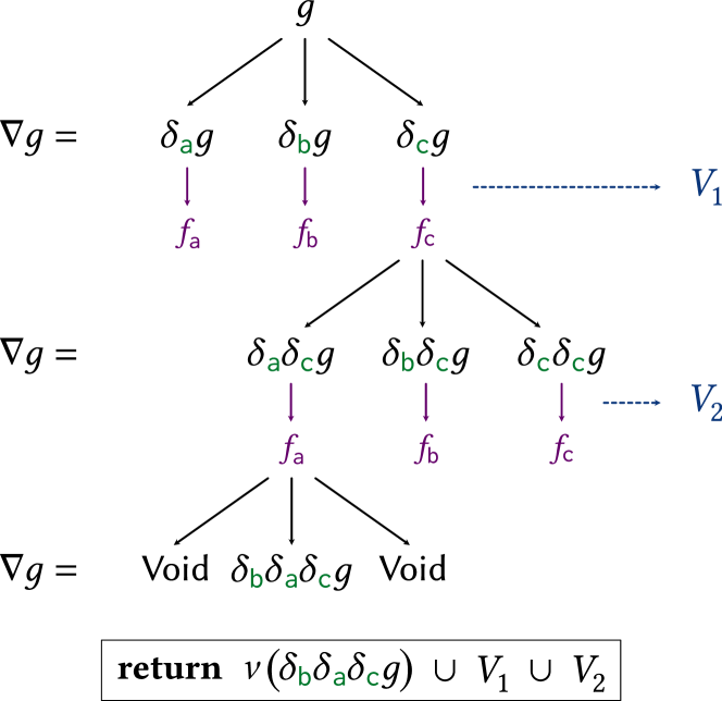
Figure 5. The main loop of Choice Gradient Sampling.

Critically, we avoid wasting effort by saving the samples ($\mathcal{V}$) that we use to evaluate the gradients. Many of those samples will be valid results that we can use, so there is no reason to throw them away.

Modified Distributions. Interestingly, this algorithm works equally well for free generators whose distributions have been replaced (as discussed in §3.5). Recall that we modify the distribution of a free generator $g$ by pairing it with a pair of a history $h$ and a distribution function $d$. We can define the derivative of such a structure to be:

⬇

$\kl[generatorderivative]{\delta}_{c}$((h, d), g) = ((h $\cdot$ c, d), $\kl[generatorderivative]{\delta}_{c}$g)

We take the derivative of $g$ and internalize $c$ into the distribution’s history. Furthermore, we can say that a modified generator’s nullable set is the same as the nullable set of the underlying generator.

These definitions, along with the ones in §3.5, are enough to replicate Choice Gradient Sampling for a free generator with an external distribution.

6. Exploratory Evaluation

This paper is primarily about the theory of [free generator]free generators and their (GEN)[derivative]derivatives, but readers may be curious (as we were) to see how well [cgs]Choice Gradient Sampling performs on a few property-based testing benchmarks. In this section, we describe some preliminary experiments in this direction; the results suggest that, with a few interesting caveats, CGS is a promising approach to the valid generation problem.

Experimental Setup. Our experiments explore how well CGS improves on the base, naïve generator by comparing it to rejection sampling, which takes a naïve generator, samples from it, and discards any results that are not valid. Rejection sampling is the default method that QuickCheck uses for properties with preconditions when no bespoke generator is available, and makes for a clean baseline that we can compare CGS to.

We use four simple free generators to test four different benchmarks: BST, SORTED, AVL, and STLC. Details about each of these benchmarks are given in Table 1.

	Free Generator	Validity Condition	$N$	Depth
BST	Binary trees with values 0–9	Is a valid BST	50	5
SORTED	Lists with values 0–9	Is sorted	50	20
AVL	Binary trees with values and stored heights 0–9	Is a valid AVL tree (balanced)	500	5
STLC	Arbitrary ASTs for $\lambda$-terms	Is well-typed	400	5

Table 1. Overview of benchmarks.

Each of our benchmarks requires a simple free generator to act as a baseline and as a starting point for CGS. For consistency, and to avoid potential biases, our generators follow the respective inductive data types as closely as possible. For example, fgenTree, shown in §3 and used in the BST benchmark, follows the structure of Tree exactly. We chose values for $N$ via trial and error in order to balance fitness accuracy with sampling time.

Results. We ran CGS and Rejection on each benchmark for one minute (on a MacBook Pro with an M1 processor and 16GB RAM) and recorded the unique valid values produced. We counted unique values because duplicate tests are generally less useful than fresh ones (in property-based testing of pure programs, in particular, duplicate tests add no value). The totals, averaged over 10 trials, are presented in Table 2.

	BST	SORTED	AVL	STLC
Rej.	$9729$ ($103$)	$6587$ ($125$)	$156$ ($5$)	$105602$ ($2501$)
CGS	$22349$ ($416$)	$58656$ ($881$)	$220$ ($1$)	$297703$ ($11726$)

Table 2. Unique valid values generated in 60 seconds ($n=10$ trials).

These measurements show that CGS is always able to generate more unique values than Rejection in the same amount of time, and it often generates significantly more. (The exception is the AVL benchmark; we discuss this below.)

Besides unique values, we measured some other metrics; the charts in Figure 6 give some deeper insights for the STLC benchmark. The first plot (“Unique Terms over Time”) shows that, after one minute, CGS has not yet begun to “run out” of unique terms to generate. Additionally “Normalized Size Distribution” chart shows that CGS also generates larger terms on average. This is good from the perspective of property-based testing, where test size is often positively correlated with bug-finding power, since larger test inputs tend to exercise more of the implementation code. Charts for the remaining benchmarks are in Appendix E.

Figure 6. Unique values and term sizes for the STLC benchmark (first trial).

Measuring Diversity. When testing, we care about more than just the number of valid test inputs generated in a period of time—we care about the diversity of those inputs, since a more diverse test suite will find more bugs more quickly.

Our diversity metric relies on the fact that each value is roughly isomorphic to the choice sequence that generated it. For example, in the case of BST, the sequence n5l6ll can be parsed to produce Node 5 Leaf (Node 6 Leaf Leaf) and a simple in-order traversal can recover n5l6ll again. Thus, choice sequence diversity is a reasonable proxy for value diversity.

We estimated the average Levenshtein distance (Levenshtein et al., 1966) (the number of edits needed to turn one string into another) between pairs of choice sequences in the values generated by each of our algorithms. Computing an exact mean distance between all pairs in such a large set would be very expensive, so we settled for the mean of a random sample of 3000 pairs from each set of valid values. The results are summarized in Table 3.

	BST	SORTED	AVL	STLC
Rej.	$7.70(1.71)$	$4.80(1.15)$	$4.42(2.01)$	$12.24(4.55)$
CGS	$8.89(1.95)$	$7.28(1.92)$	$4.35(1.98)$	$13.62(4.72)$

Table 3. Average Levenshtein distance between pairs of choice sequences (first trial).

While SORTED does see significantly improved diversity, the effect is less dramatic STLC and BST, and diversity for AVL actually gets slightly worse.

One explanation for these lackluster results rests on the way CGS retains intermediate samples. While the first few samples will be mostly uncorrelated, the samples drawn later on in the generation process (once a number of choices have been fixed) will tend to be similar to one another. This likely results in some clusters of inputs that are all valid but that only explore one particular shape of input.

Of course, is already common practice to test clusters of similar inputs in certain fuzzing contexts (Lampropoulos et al., 2019), so the fact that CGS does this is not unusual. In fact, this method has been shown to be effective at finding bugs in some cases. Additionally, for most of our benchmarks (again, we return to AVL in a moment) CGS does increase diversity of tests; combined with the sheer number of valid inputs available, this means that CGS covers a slightly larger space of tests much more thoroughly. This effect should lead to better bug-finding in testing scenarios.

The Problem with AVL. The AVL benchmark is an outlier in most of these measurements: CGS only manages to find a modest number of extra valid AVL trees, and their pairwise diversity is actually slightly worse than that of rejection sampling. Why might this be? We suspect that this effect arises because AVL trees are quite difficult to find randomly. Balanced binary search trees are hard to generate on their own, and AVL trees are even more difficult because the generator must guess the correct height to cache at each node. This is why rejection sampling only finds $156$ AVL trees in the time it takes to find $9762$ binary search trees.

This all means that CGS is unlikely find any valid trees while sampling. In particular, the check in line 15 of Figure 5 will often be true, meaning that choices will be made uniformly at random rather than guided by the fitness of the appropriate derivatives. We could reduce this effect by significantly increasing the sample rate constant $N$, but then sampling time would likely dominate generation time, resulting in worse performance overall.

The lesson here seems to be that the CGS algorithm does not work well with especially hard-to-satisfy predicates. In §8, we present an idea that would do some of the hard work ahead of time and help with this issue, but clearly many predicates (including complex ones like well-typedness of STLC terms) are within reach of the current algorithm. Indeed, as long as every $N$ samples from the naïve generator has at least a few valid values on average, the AVL issue will not come up. We expect that many real-world structural and semantic constraints will require a small enough $N$ for CGS to be effective.

7. Related Work

We discuss a number of approaches that are similar to ours, via either connections to free generators or connections to our Choice Gradient Sampling algorithm.

Parsing and Generation. The connection between parsers and generators is not just “intellectual folklore”—it is used in some implementations too. At least two popular property-based testing libraries, Hypothesis (MacIver et al., 2019) and Crowbar (Dolan and Preston, 2017), implement generators by parsing a stream of random bits (and there may very well be others that we do not know of.) This further illustrates the value in formalizing the connection between parsers and generators, as a way to explain existing implementations uncover potential opportunities.

The Clotho (Darragh et al., 2021) library introduces “parametric randomness,” providing a way to carefully control generator choices from outside of the generator. While Darragh et al. do not use parsing in their formalism, it is still exciting to see others considering the implications of controlling generator choices externally.

Free Applicative Generators. Claessen et al. (2015) present a generator representation that is structurally similar to our free generators, but which is used in a very different way. They primarily use the syntactic structure of their generators (they call them “spaces”) to control the size distribution of generated outputs; in particular, spaces do not make choice information explicit in the way free generators do. Claessen et al.’s generation approach uses Haskell’s laziness, rather than derivatives and sampling, to prune unhelpful paths in the generation process. This pruning procedure performs well when validity conditions are written to take advantage of laziness, but it is highly dependent on evaluation order and it does not differentiate between generator choices that are not obviously bad. In contrast, CGS respects observational equivalence between predicates and uses sampling to weight next choices.

The Valid Generation Problem. Many other approaches to the valid generation problem have been explored.

The domain-specific language for generators provided by the QuickCheck library (Hughes, 2007) makes it easier to write manual generators that produce valid inputs by construction. This approach is extremely general, but it can be labor intensive. In the present work, we avoid manual techniques like this in the hopes of making property-based testing more accessible to programmers that do not have the time or expertise to write their own custom generators.

The Luck (Lampropoulos et al., 2017a) language provides a sort of middle-ground solution; users are still required to put in some effort, but they are able to define generators and validity predicates at the same time. Luck provides a satisfying solution if users are starting from scratch and willing to learn a domain-specific language, but if validity predicates have already been written or users do not want to learn a new language, a more automated solution is preferable.

When validity predicates are expressed as inductive relations, approaches like the one in Generating Good Generators for Inductive Relations (Lampropoulos et al., 2017b) are extremely powerful. Unfortunately, most programming languages cannot express inductive relations that capture the kinds of preconditions that we care about.

Target (Löscher and Sagonas, 2017) uses search strategies like hill-climbing and simulated annealing to supplement random generation and significantly streamline property-based testing. Löscher and Sagonas’s approach works extremely well when inputs have a sensible notion of “utility,” but in the case of valid generation the utility is often degenerate—0 if the input is invalid, and 1 if it is valid—with no good way to say if an input is “better” or “worse.” In these cases, derivative-based searches may make more sense.

Some approaches use machine learning to automatically generate valid inputs. Learn&Fuzz (Godefroid et al., 2017) generates valid data using a recurrent neural network. While the results are promising, this solution seems to work best when a large corpus of inputs is already available and the validity condition is more structural than semantic. In the same vein, RLCheck (Reddy et al., 2020) uses reinforcement learning to guide a generator to valid inputs. This approach served as early inspiration for our work, and we think that the theoretical advance of generator derivatives may lead improved learning algorithms in the future (see §8).

8. Future Directions

There are a number of exciting paths forward from this work; some continue our theoretical exploration and others look towards algorithmic improvements.

Bidirectional Free Generators. We believe that we have only scratched the surface of what is possible with [free generator]free generators. One concrete next step is to merge the theory of free generators with the emerging theory of ungenerators (Goldstein, 2021). Goldstein expresses generators that can be run both forward (to generate values as usual) and backward. In the backward direction, the program takes a value that the generator might have generated and “un-generates” it to give a sequence of choices that the generator might have made when generating that value.

Free generators are quite compatible with these ideas, and turning a free generator into a bidirectional generator that can both generate and ungenerate should be fairly straightforward. From there, we can build on the ideas in the ungenerators work and use the backward direction of the generator to learn a distribution of choices that approximates some user-provided samples of “desirable” values. Used in conjunction with the extended algorithm from §5, this would give a better starting point for generation with little extra work from the user.

Algorithmic Optimizations. In §3, we saw some problems with the [cgs]Choice Gradient Sampling algorithm: because CGS evaluates derivatives via sampling, it does poorly when validity conditions are particularly difficult to satisfy. This begs the question: might it be possible to evaluate the fitness of a derivative without naïvely sampling?

One potential angle involves staging the sampling process. Given a free generator with a depth parameter, we can first evaluate choices on generators of size 1, then evaluate choices with size 2, etc. These intermediate stages would make gradient sampling more successful at larger sizes, and might significantly improve the results on benchmarks like AVL. Unfortunately, this kind of approach might perform poorly on benchmarks like STLC where the validity condition is not uniform: size-1 generators would avoid generating variables, leading larger generators to avoid variables as well. In any case, we think this design space is worth exploring.

Making Choices with Neural Networks. Another algorithmic optimization is a bit farther afield: we think it may be possible to use recurrent neural networks (RNNs) to improve our generation procedure.

As Choice Gradient Sampling makes choices, it generates useful data about the frequencies with which choices should be made. Specifically, every iteration of the algorithm produces a pair of a history and a distribution over next choices that looks something like

$${\color[rgb]{0.0078125,0.46875,0.17578125}\tt abcca}\mapsto\{{\color[rgb]{0.0078125,0.46875,0.17578125}\tt a}:0.3,{\color[rgb]{0.0078125,0.46875,0.17578125}\tt b}:0.7,{\color[rgb]{0.0078125,0.46875,0.17578125}\tt c}:0.0\}.$$

In the course of CGS, this information is used once (to make the next choice) and then forgotten—what if there was a way to learn from it? Pairs like this could be used to train an RNN to make choices that are similar to the ones made by CGS.

There are still details to work out, including network architecture, hyper-parameters, etc., but in theory we could run CGS for a while, then train the model, and after that point only use the RNN to generate valid data. Setting things up this way would recover some of the time that is currently wasted by the constant sampling of derivative generators.

One could imagine a user writing a definition of a type and a predicate for that type, and then setting the model to train while they work on their algorithm. By the time the algorithm is finished and ready to test, the RNN model would be trained and ready to produce valid test inputs. A workflow like this could significantly increase adoption of property-based testing in industry.

Free generators and their derivatives are powerful structures that give a unique and flexible perspective on random generation. Our formalism yields a useful algorithm and clarifies the folklore that a generator is a parser of randomness.

Appendix

Appendix A Proof of Lemma 4.1

Lemma 4.1.

If a free generator $g$ is in simplified form, then either ${g=\text{\leavevmode\lstinline{{\lst@@@set@language\lst@@@set@numbers\lst@@@set@frame\lst@@@set@rulecolor{\@listingGroup{ltx_lst_identifier}{Pure}}{\@listingGroup{ltx_lst_space}{ }}{\@listingGroup{ltx_lst_identifier}{a}}}}}}$ or $\varepsilon\notin\kl[languageofafreegenerator]{\mathcal{L}}\llbracket{}g\rrbracket{}$.

Proof.

We proceed by induction on the structure of $g$.

• $g=\textsf{Void}$. Trivial.

• $g=\textsf{Pure a}$. Trivial.

• $g=\textsf{Pair x y}$. By our inductive hypothesis, $x=\textsf{Pure a}$ or $\varepsilon\notin\kl[languageofafreegenerator]{\mathcal{L}}\llbracket{}\textsf{x}\rrbracket{}$.

  Since the smart constructor $\otimes$ never constructs a Pair with Pure on the left, it must be that $\varepsilon\notin\kl[languageofafreegenerator]{\mathcal{L}}\llbracket{}\textsf{x}\rrbracket{}$.

  Therefore, it must be the case that $\varepsilon\notin\kl[languageofafreegenerator]{\mathcal{L}}\llbracket{}\textsf{Pair x y}\rrbracket{}$.

• $g=\textsf{Map f x}$.

  Similarly to the previous case, our inductive hypothesis and simplification assumptions imply that $\varepsilon\notin\kl[languageofafreegenerator]{\mathcal{L}}\llbracket{}\textsf{x}\rrbracket{}$.

  Therefore, $\varepsilon\notin\kl[languageofafreegenerator]{\mathcal{L}}\llbracket{}\textsf{Map f y}\rrbracket{}$.

• $g=\textsf{Select xs}$.

  It is always the case that $\varepsilon\notin\kl[languageofafreegenerator]{\mathcal{L}}\llbracket{}\textsf{Select xs}\rrbracket{}$.

Thus, we have shown that every simplified free generator is either Pure a or cannot accept the empty string. ∎

Appendix B Proof of Theorem 3.4

Lemma B.1.

Pairing two [parser interpretation]parser interpretations and mapping over the concatenation of the associated choice distributions is equal to a function of the two parsers mapped over the distributions individually. Specifically, for all [simplified form]simplified [free generator]free generators x and y,

$$((\lambda x\ y\to(x,y))\operatorname{\kl[functor]{\langle{}\${}\rangle{}}}\kl[parserinterpretation]{\mathcal{P}}\llbracket{}\textsf{x}\rrbracket{}\operatorname{\kl[applicative]{\langle{}\!\!\ast{}\!\!\rangle{}}}\kl[parserinterpretation]{\mathcal{P}}\llbracket{}\textsf{y}\rrbracket{})\operatorname{\kl[functor]{\langle{}\${}\rangle{}}}((\cdot)\operatorname{\kl[functor]{\langle{}\${}\rangle{}}}\kl[choicedistribution]{\mathcal{C}}\llbracket{}\textsf{x}\rrbracket{}\operatorname{\kl[applicative]{\langle{}\!\!\ast{}\!\!\rangle{}}}\kl[choicedistribution]{\mathcal{C}}\llbracket{}\textsf{y}\rrbracket{}) \operatorname{\kl[generatorequivalence]{\equiv}}(\lambda a_{\bot}\ b_{\bot}\to\textbf{{case}}~{}(a_{\bot},b_{\bot})~{}\textbf{{of}}$$

$$\quad\quad(\textsf{Just}~{}(a,\_),\textsf{Just}~{}(b,\_))\to\textsf{Just}~{}((a,b),\varepsilon)$$

$$\quad\quad\_\to\textsf{Nothing})$$

$$\quad\operatorname{\kl[functor]{\langle{}\${}\rangle{}}}(\kl[parserinterpretation]{\mathcal{P}}\llbracket{}\textsf{x}\rrbracket{}\operatorname{\kl[functor]{\langle{}\${}\rangle{}}}\kl[choicedistribution]{\mathcal{C}}\llbracket{}\textsf{x}\rrbracket{})\operatorname{\kl[applicative]{\langle{}\!\!\ast{}\!\!\rangle{}}}(\kl[parserinterpretation]{\mathcal{P}}\llbracket{}\textsf{y}\rrbracket{}\operatorname{\kl[functor]{\langle{}\${}\rangle{}}}\kl[choicedistribution]{\mathcal{C}}\llbracket{}\textsf{y}\rrbracket{})$$

Proof.

First, note that for any simplified generator, $g$, if $\kl[choicedistribution]{\mathcal{C}}\llbracket{}g\rrbracket{}$ generates a string $s$, for any other string $t$ $\kl[parserinterpretation]{\mathcal{P}}\llbracket{}g\rrbracket{}~{}(s\cdot t)=\textsf{Just}~{}(a,t)$ for some value $a$. This can be shown by induction on the structure of $g$.

Now, assume $\kl[choicedistribution]{\mathcal{C}}\llbracket{}\textsf{x}\rrbracket{}$ generates a string $s$, and $\kl[choicedistribution]{\mathcal{C}}\llbracket{}\textsf{y}\rrbracket{}$ generates $t$. This means that $(\cdot)\operatorname{\kl[functor]{\langle{}\${}\rangle{}}}\kl[choicedistribution]{\mathcal{C}}\llbracket{}\textsf{x}\rrbracket{}\operatorname{\kl[applicative]{\langle{}\!\!\ast{}\!\!\rangle{}}}\kl[choicedistribution]{\mathcal{C}}\llbracket{}\textsf{y}\rrbracket{}$ generates $s\cdot t$.

By the above fact, it is simple to show that both sides of the above equation simplify to $\textsf{Just}~{}((a,b),\varepsilon)$ for some values $a$ and $b$ that depend on the particular interpretations of x and y.

Since this is true for any $s$ and $t$ that the choice distributions generate, the desired fact holds. ∎

Theorem 3.4.

Every [simplified form]simplified free generator can be factored into a parser and a distribution over choice sequences. In other words, for all simplified free generators $g\neq\textsf{Void}$,

$$\kl[parserinterpretation]{\mathcal{P}}\llbracket{}g\rrbracket{}\operatorname{\kl[functor]{\langle{}\${}\rangle{}}}\kl[choicedistribution]{\mathcal{C}}\llbracket{}g\rrbracket{}\operatorname{\kl[generatorequivalence]{\equiv}}(\lambda x\to\textsf{Just}~{}(x,\varepsilon))\operatorname{\kl[functor]{\langle{}\${}\rangle{}}}\kl[generatorinterpretation]{\mathcal{G}}\llbracket{}g\rrbracket{}.$$

Proof.

We proceed by induction on the structure of $g$.

• $g=\textsf{Pure a}$.

  $$\kl[parserinterpretation]{\mathcal{P}}\llbracket{}\textsf{Pure a}\rrbracket{}\operatorname{\kl[functor]{\langle{}\${}\rangle{}}}\kl[choicedistribution]{\mathcal{C}}\llbracket{}\textsf{Pure a}\rrbracket{} \operatorname{\kl[generatorequivalence]{\equiv}}\textsf{pure}~{}(\textsf{Just}~{}(\textsf{a},\varepsilon))$$ (by defn)

  $$\operatorname{\kl[generatorequivalence]{\equiv}}(\lambda x\to\textsf{Just}~{}(x,\varepsilon))\operatorname{\kl[functor]{\langle{}\${}\rangle{}}}\kl[generatorinterpretation]{\mathcal{G}}\llbracket{}\textsf{Pure a}\rrbracket{}$$ (by defn)

• $g=\textsf{Pair x y}$.

  $$\kl[parserinterpretation]{\mathcal{P}}\llbracket{}\textsf{Pair x y}\rrbracket{}\operatorname{\kl[functor]{\langle{}\${}\rangle{}}}\kl[choicedistribution]{\mathcal{C}}\llbracket{}\textsf{Pair x y}\rrbracket{} \operatorname{\kl[generatorequivalence]{\equiv}}((\lambda x\ y\to(x,y))\operatorname{\kl[functor]{\langle{}\${}\rangle{}}}\kl[parserinterpretation]{\mathcal{P}}\llbracket{}\textsf{x}\rrbracket{}\operatorname{\kl[applicative]{\langle{}\!\!\ast{}\!\!\rangle{}}}\kl[parserinterpretation]{\mathcal{P}}\llbracket{}\textsf{y}\rrbracket{})\operatorname{\kl[functor]{\langle{}\${}\rangle{}}}((\cdot)\operatorname{\kl[functor]{\langle{}\${}\rangle{}}}\kl[choicedistribution]{\mathcal{C}}\llbracket{}\textsf{x}\rrbracket{}\operatorname{\kl[applicative]{\langle{}\!\!\ast{}\!\!\rangle{}}}\kl[choicedistribution]{\mathcal{C}}\llbracket{}\textsf{y}\rrbracket{})$$ (by defn)

  $$\operatorname{\kl[generatorequivalence]{\equiv}}(\lambda a_{\bot}\ b_{\bot}\to\textbf{{case}}~{}(a_{\bot},b_{\bot})~{}\textbf{{of}}$$

  $$\quad\quad(\textsf{Just}~{}(a,\_),\textsf{Just}~{}(b,\_))\to\textsf{Just}~{}((a,b),\varepsilon)$$

  $$\quad\quad\_\to\textsf{Nothing})$$

  $$\quad\operatorname{\kl[functor]{\langle{}\${}\rangle{}}}(\kl[parserinterpretation]{\mathcal{P}}\llbracket{}\textsf{x}\rrbracket{}\operatorname{\kl[functor]{\langle{}\${}\rangle{}}}\kl[choicedistribution]{\mathcal{C}}\llbracket{}\textsf{x}\rrbracket{})\operatorname{\kl[applicative]{\langle{}\!\!\ast{}\!\!\rangle{}}}(\kl[parserinterpretation]{\mathcal{P}}\llbracket{}\textsf{y}\rrbracket{}\operatorname{\kl[functor]{\langle{}\${}\rangle{}}}\kl[choicedistribution]{\mathcal{C}}\llbracket{}\textsf{y}\rrbracket{})$$ (by Lemma B.1)

  $$\operatorname{\kl[generatorequivalence]{\equiv}}(\lambda a_{\bot}\ b_{\bot}\to\textbf{{case}}~{}(a_{\bot},b_{\bot})~{}\textbf{{of}}$$

  $$\quad\quad(\textsf{Just}~{}(a,\_),\textsf{Just}~{}(b,\_))\to\textsf{Just}~{}((a,b),\varepsilon)$$

  $$\quad\quad\_\to\textsf{Nothing})$$

  $$\quad\operatorname{\kl[functor]{\langle{}\${}\rangle{}}}((\lambda x\to\textsf{Just}~{}(x,\varepsilon))\operatorname{\kl[functor]{\langle{}\${}\rangle{}}}\kl[generatorinterpretation]{\mathcal{G}}\llbracket{}\textsf{x}\rrbracket{})\operatorname{\kl[applicative]{\langle{}\!\!\ast{}\!\!\rangle{}}}((\lambda x\to\textsf{Just}~{}(x,\varepsilon))\operatorname{\kl[functor]{\langle{}\${}\rangle{}}}\kl[generatorinterpretation]{\mathcal{G}}\llbracket{}\textsf{y}\rrbracket{})$$ (by IH)

  $$\operatorname{\kl[generatorequivalence]{\equiv}}(\lambda x\to\textsf{Just}~{}(x,\varepsilon))\operatorname{\kl[functor]{\langle{}\${}\rangle{}}}((\lambda x\ y\to(x,y))\operatorname{\kl[functor]{\langle{}\${}\rangle{}}}\kl[generatorinterpretation]{\mathcal{G}}\llbracket{}\textsf{x}\rrbracket{}\operatorname{\kl[applicative]{\langle{}\!\!\ast{}\!\!\rangle{}}}\kl[generatorinterpretation]{\mathcal{G}}\llbracket{}\textsf{y}\rrbracket{})$$ (by app. properties)

  $$\operatorname{\kl[generatorequivalence]{\equiv}}(\lambda x\to\textsf{Just}~{}(x,\varepsilon))\operatorname{\kl[functor]{\langle{}\${}\rangle{}}}\kl[generatorinterpretation]{\mathcal{G}}\llbracket{}\textsf{Pair x y}\rrbracket{}$$ (by defn)

• $g=\textsf{Map f x}$.

  $$\kl[parserinterpretation]{\mathcal{P}}\llbracket{}\textsf{Map f x}\rrbracket{}\operatorname{\kl[functor]{\langle{}\${}\rangle{}}}\kl[choicedistribution]{\mathcal{C}}\llbracket{}\textsf{Map f x}\rrbracket{} \operatorname{\kl[generatorequivalence]{\equiv}}(\textsf{f}\operatorname{\kl[functor]{\langle{}\${}\rangle{}}}\kl[parserinterpretation]{\mathcal{P}}\llbracket{}\textsf{x}\rrbracket{})\operatorname{\kl[functor]{\langle{}\${}\rangle{}}}\kl[choicedistribution]{\mathcal{C}}\llbracket{}x\rrbracket{}$$ (by defn)

  $$\operatorname{\kl[generatorequivalence]{\equiv}}\textsf{f}\operatorname{\kl[functor]{\langle{}\${}\rangle{}}}(\kl[parserinterpretation]{\mathcal{P}}\llbracket{}\textsf{x}\rrbracket{}\operatorname{\kl[functor]{\langle{}\${}\rangle{}}}\kl[choicedistribution]{\mathcal{C}}\llbracket{}x\rrbracket{})$$ (by functor properties)

  $$\operatorname{\kl[generatorequivalence]{\equiv}}\textsf{f}\operatorname{\kl[functor]{\langle{}\${}\rangle{}}}((\lambda x\to\textsf{Just}~{}(x,\varepsilon))\operatorname{\kl[functor]{\langle{}\${}\rangle{}}}\kl[generatorinterpretation]{\mathcal{G}}\llbracket{}\textsf{x}\rrbracket{})$$ (by IH)

  $$\operatorname{\kl[generatorequivalence]{\equiv}}(\lambda x\to\textsf{Just}~{}(x,\varepsilon))\operatorname{\kl[functor]{\langle{}\${}\rangle{}}}(\textsf{f}\operatorname{\kl[functor]{\langle{}\${}\rangle{}}}\kl[generatorinterpretation]{\mathcal{G}}\llbracket{}\textsf{x}\rrbracket{})$$ (by functor properties)

  $$\operatorname{\kl[generatorequivalence]{\equiv}}(\lambda x\to\textsf{Just}~{}(x,\varepsilon))\operatorname{\kl[functor]{\langle{}\${}\rangle{}}}\kl[generatorinterpretation]{\mathcal{G}}\llbracket{}\textsf{Map f x}\rrbracket{}$$ (by defn)

• $g=\textsf{Select xs}$.

  $$\kl[parserinterpretation]{\mathcal{P}}\llbracket{}\textsf{Select xs}\rrbracket{}\operatorname{\kl[functor]{\langle{}\${}\rangle{}}}\kl[choicedistribution]{\mathcal{C}}\llbracket{}\textsf{Select xs}\rrbracket{} \operatorname{\kl[generatorequivalence]{\equiv}}(\textsf{choice}~{}(\textsf{map}~{}(\lambda(c,\textsf{x})\to(c,\kl[parserinterpretation]{\mathcal{P}}\llbracket{}\textsf{x}\rrbracket{}))~{}\textsf{xs}))$$

  $$\quad\operatorname{\kl[functor]{\langle{}\${}\rangle{}}}\textsf{oneof}~{}(\textsf{map}~{}(\lambda(c,\textsf{x})\to(c\cdot)\operatorname{\kl[functor]{\langle{}\${}\rangle{}}}\kl[choicedistribution]{\mathcal{C}}\llbracket{}\textsf{x}\rrbracket{})~{}\textsf{xs})$$ (by defn)

  $$\operatorname{\kl[generatorequivalence]{\equiv}}\textsf{oneof}~{}(\textsf{map}~{}(\lambda(c,\textsf{x})\to$$

  $$\quad\quad(\textsf{choice}~{}(\textsf{map}~{}(\lambda(c,\textsf{x})\to(c,\kl[parserinterpretation]{\mathcal{P}}\llbracket{}\textsf{x}\rrbracket{}))~{}\textsf{xs}))\circ(c\cdot)\operatorname{\kl[functor]{\langle{}\${}\rangle{}}}\kl[choicedistribution]{\mathcal{C}}\llbracket{}\textsf{x}\rrbracket{}$$

  $$\quad)~{}\textsf{xs})$$ (by generator properties)

  $$\operatorname{\kl[generatorequivalence]{\equiv}}\textsf{oneof}~{}(\textsf{map}~{}(\lambda(\_,\textsf{x})\to\kl[parserinterpretation]{\mathcal{P}}\llbracket{}\textsf{x}\rrbracket{}\operatorname{\kl[functor]{\langle{}\${}\rangle{}}}\kl[choicedistribution]{\mathcal{C}}\llbracket{}\textsf{x}\rrbracket{})~{}\textsf{xs})$$ (by parser properties)

  $$\operatorname{\kl[generatorequivalence]{\equiv}}\textsf{oneof}~{}(\textsf{map}~{}(\lambda(\_,\textsf{x})\to(\lambda x\to\textsf{Just}~{}(x,\varepsilon))\operatorname{\kl[functor]{\langle{}\${}\rangle{}}}\kl[generatorinterpretation]{\mathcal{G}}\llbracket{}\textsf{x}\rrbracket{})~{}\textsf{xs})$$ (by IH)

  $$\operatorname{\kl[generatorequivalence]{\equiv}}(\lambda x\to\textsf{Just}~{}(x,\varepsilon))\operatorname{\kl[functor]{\langle{}\${}\rangle{}}}\textsf{oneof}~{}(\textsf{map}~{}(\lambda(\_,\textsf{x})\to\kl[generatorinterpretation]{\mathcal{G}}\llbracket{}\textsf{x}\rrbracket{})~{}\textsf{xs})$$ (by generator properties)

  $$\operatorname{\kl[generatorequivalence]{\equiv}}(\lambda x\to\textsf{Just}~{}(x,\varepsilon))\operatorname{\kl[functor]{\langle{}\${}\rangle{}}}\kl[generatorinterpretation]{\mathcal{G}}\llbracket{}\textsf{Select xs}\rrbracket{}$$ (by defn)

Thus, generators can be coherently factored into a parser and a distribution. ∎

Appendix C Proof of Theorem 4.2

Theorem 4.2.

For all [simplified form]simplified [free generator]free generators $g$ and choices $c$,

$$\delta_{c}\kl[languageofafreegenerator]{\mathcal{L}}\llbracket{}g\rrbracket{}=\kl[languageofafreegenerator]{\mathcal{L}}\llbracket{}\kl[generatorderivative]{\delta}_{c}g\rrbracket{}.$$

Proof.

We again proceed by induction on the structure of $g$.

• $g=\textsf{Void}$. $\varnothing=\varnothing$.

• $g=\textsf{Pure a}$. $\varnothing=\varnothing$.

• $g=\textsf{Pair x y}$.

  $$\delta_{c}\kl[languageofafreegenerator]{\mathcal{L}}\llbracket{}\textsf{Pair x y}\rrbracket{} =\delta_{c}(\kl[languageofafreegenerator]{\mathcal{L}}\llbracket{}\textsf{x}\rrbracket{}\cdot\kl[languageofafreegenerator]{\mathcal{L}}\llbracket{}\textsf{y}\rrbracket{})$$ (by defn)

  $$=\delta_{c}(\kl[languageofafreegenerator]{\mathcal{L}}\llbracket{}\textsf{x}\rrbracket{})\cdot\kl[languageofafreegenerator]{\mathcal{L}}\llbracket{}\textsf{y}\rrbracket{}+\nu\kl[languageofafreegenerator]{\mathcal{L}}\llbracket{}\textsf{x}\rrbracket{}\cdot\delta_{c}\kl[languageofafreegenerator]{\mathcal{L}}\llbracket{}\textsf{y}\rrbracket{}$$ (by defn)

  $$=\delta_{c}(\kl[languageofafreegenerator]{\mathcal{L}}\llbracket{}\textsf{x}\rrbracket{})\cdot\kl[languageofafreegenerator]{\mathcal{L}}\llbracket{}\textsf{y}\rrbracket{}$$ (by Lemma 4.1)

  $$=\kl[languageofafreegenerator]{\mathcal{L}}\llbracket{}\kl[generatorderivative]{\delta}_{c}\textsf{x}\rrbracket{}\cdot\kl[languageofafreegenerator]{\mathcal{L}}\llbracket{}\textsf{y}\rrbracket{}$$ (by IH)

  $$=\kl[languageofafreegenerator]{\mathcal{L}}\llbracket{}\textsf{Pair}~{}(\kl[generatorderivative]{\delta}_{c}\textsf{x})~{}\textsf{y}\rrbracket{}$$ (by defn)

  $$=\kl[languageofafreegenerator]{\mathcal{L}}\llbracket{}\kl[generatorderivative]{\delta}_{c}\textsf{Pair x y}\rrbracket{}$$ (by defn)

• $g=\textsf{Map f x}$.

  $$\delta_{c}\kl[languageofafreegenerator]{\mathcal{L}}\llbracket{}\textsf{Map f x}\rrbracket{} =\delta_{c}\kl[languageofafreegenerator]{\mathcal{L}}\llbracket{}\textsf{x}\rrbracket{}$$ (by defn)

  $$=\kl[languageofafreegenerator]{\mathcal{L}}\llbracket{}\kl[generatorderivative]{\delta}_{c}\textsf{x}\rrbracket{}$$ (by IH)

  $$=\kl[languageofafreegenerator]{\mathcal{L}}\llbracket{}\textsf{Map f}~{}(\kl[generatorderivative]{\delta}_{c}\textsf{x})\rrbracket{}$$ (by defn)

  $$=\kl[languageofafreegenerator]{\mathcal{L}}\llbracket{}\kl[generatorderivative]{\delta}_{c}(\textsf{Map f x})\rrbracket{}$$ (by defn*)

  *Note that the last step follows because Map f x is assumed to be simplified, so $x\neq\textsf{Pure a}$. This means that f $\operatorname{\kl[functor]{\langle{}\${}\rangle{}}}$ x is equivalent to Map f x.

• $g=\textsf{Select xs}$. If there is no pair (c, x) in xs, then $\varnothing=\varnothing$. Otherwise,

  $$\delta_{c}\kl[languageofafreegenerator]{\mathcal{L}}\llbracket{}\textsf{Select xs}\rrbracket{} =\delta_{c}\{c\cdot s\mid s\in\kl[languageofafreegenerator]{\mathcal{L}}\llbracket{}\textsf{x}\rrbracket{}\}$$ (by defn)

  $$=\kl[languageofafreegenerator]{\mathcal{L}}\llbracket{}\textsf{x}\rrbracket{}$$ (by defn)

  $$=\kl[languageofafreegenerator]{\mathcal{L}}\llbracket{}\kl[generatorderivative]{\delta}_{c}(\textsf{Select xs})\rrbracket{}$$ (by defn)

Thus we have shown that the symbolic derivative of free generators is compatible with the derivative of the generator’s language. ∎

There is another proof of this theorem, suggested by Alexandra Silva, which uses the fact that $2^{\Sigma^{*}}$ is the final coalgebra, along with the observation that FGen has a $2\times{(-)}^{\Sigma}$ coalgebraic structure. This approach is certainly more elegant, but it abstracts away some helpful operational intuition.

Appendix D Proof of Theorem 4.3

Theorem 4.3.

For all [simplified form]simplified [free generator]free generators $g$, choice sequences $s$, and choices $c$,

$$\kl[parserinterpretation]{\mathcal{P}}\llbracket{}\kl[generatorderivative]{\delta}_{c}{g}\rrbracket{}~{}s=\kl[parserinterpretation]{\mathcal{P}}\llbracket{}g\rrbracket{}~{}(c\cdot s).$$

Proof.

For simplicity, we prove the point-free version of this claim, i.e.:

$$\kl[parserinterpretation]{\mathcal{P}}\llbracket{}\kl[generatorderivative]{\delta}_{c}{g}\rrbracket{}=\kl[parserinterpretation]{\mathcal{P}}\llbracket{}g\rrbracket{}\circ(c\cdot)$$

We proceed by induction on $g$.

• $g=\textsf{Void}$. $\textsf{Nothing}=\textsf{Nothing}$.

• $g=\textsf{Pure a}$. $\textsf{Nothing}=\textsf{Nothing}$.

• $g=\textsf{Pair x y}$.

  $$\kl[parserinterpretation]{\mathcal{P}}\llbracket{}\kl[generatorderivative]{\delta}_{c}{(\textsf{Pair x y})}\rrbracket{} =\kl[parserinterpretation]{\mathcal{P}}\llbracket{}\kl[generatorderivative]{\delta}_{c}{\textsf{x}}\otimes\textsf{y}\rrbracket{}$$ (by defn)

  $$=(\lambda x~{}y\to(x,y))\operatorname{\kl[functor]{\langle{}\${}\rangle{}}}\kl[parserinterpretation]{\mathcal{P}}\llbracket{}\kl[generatorderivative]{\delta}_{c}{\textsf{x}}\rrbracket{}\operatorname{\kl[applicative]{\langle{}\!\!\ast{}\!\!\rangle{}}}\kl[parserinterpretation]{\mathcal{P}}\llbracket{}\textsf{y}\rrbracket{}$$ (by defn)

  $$=((\lambda x~{}y\to(x,y))\operatorname{\kl[functor]{\langle{}\${}\rangle{}}}\kl[parserinterpretation]{\mathcal{P}}\llbracket{}\textsf{x}\rrbracket{}\operatorname{\kl[applicative]{\langle{}\!\!\ast{}\!\!\rangle{}}}\kl[parserinterpretation]{\mathcal{P}}\llbracket{}\textsf{y}\rrbracket{})\circ(c\cdot)$$ (by IH & Lemma 4.1*)

  $$=\kl[parserinterpretation]{\mathcal{P}}\llbracket{}\textsf{Pair x y}\rrbracket{}~{}(c\cdot)$$ (by defn)

  *We can use Lemma 4.1 to show that x must consume at least one character. Thus, we can move the $c$ in the derivative out into the final string, and trust that x will consume it.

• $g=\textsf{Map f x}$.

  $$\kl[parserinterpretation]{\mathcal{P}}\llbracket{}\kl[generatorderivative]{\delta}_{c}{(\textsf{Map f x})}\rrbracket{} =\kl[parserinterpretation]{\mathcal{P}}\llbracket{}f\operatorname{\kl[functor]{\langle{}\${}\rangle{}}}\kl[generatorderivative]{\delta}_{c}{\textsf{x}}\rrbracket{}$$ (by defn)

  $$=f\operatorname{\kl[functor]{\langle{}\${}\rangle{}}}\kl[parserinterpretation]{\mathcal{P}}\llbracket{}\kl[generatorderivative]{\delta}_{c}{\textsf{x}}\rrbracket{}$$ (by app. properties)

  $$=f\operatorname{\kl[functor]{\langle{}\${}\rangle{}}}(\kl[parserinterpretation]{\mathcal{P}}\llbracket{}\textsf{x}\rrbracket{}\circ(c\cdot))$$ (by IH)

  $$=(f\operatorname{\kl[functor]{\langle{}\${}\rangle{}}}\kl[parserinterpretation]{\mathcal{P}}\llbracket{}\textsf{x}\rrbracket{})\circ(c\cdot)$$ (by app. properties)

  $$=\kl[parserinterpretation]{\mathcal{P}}\llbracket{}\textsf{Map f x}\rrbracket{}\circ(c\cdot)$$ (by defn)

• $g=\textsf{Select xs}$. Since both the derivative and the parser simply choose the branch of the Select corresponding to $c$, this case is trivial.

∎

Appendix E Full Experimental Results

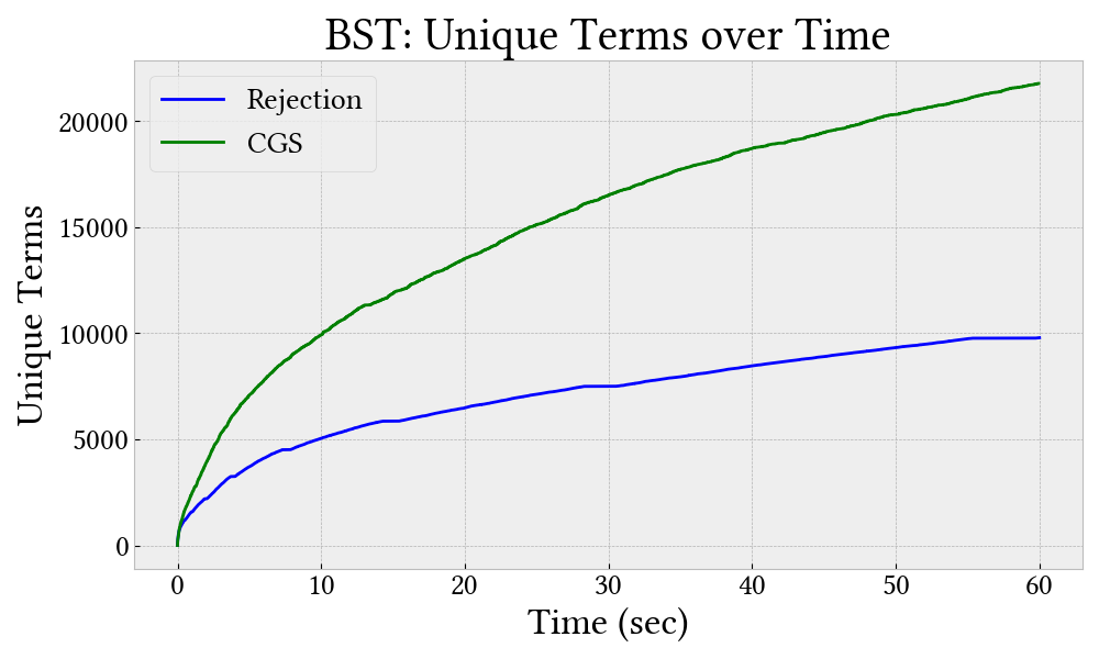
BST Charts

SORTED Charts

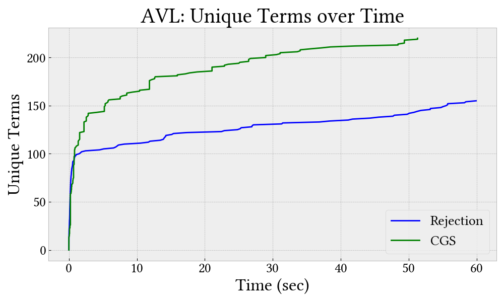
AVL Charts

References

- (1)
- Brzozowski (1964) Janusz A Brzozowski. 1964. Derivatives of regular expressions. Journal of the ACM (JACM) 11, 4 (1964), 481–494.
- Capriotti and Kaposi (2014) Paolo Capriotti and Ambrus Kaposi. 2014. Free applicative functors. arXiv preprint arXiv:1403.0749 (2014).
- Claessen et al. (2015) Koen Claessen, Jonas Duregård, and Michal H. Palka. 2015. Generating constrained random data with uniform distribution. J. Funct. Program. 25 (2015). https://doi.org/10.1017/S0956796815000143
- Claessen and Hughes (2000) Koen Claessen and John Hughes. 2000. QuickCheck: a lightweight tool for random testing of Haskell programs. In Proceedings of the Fifth ACM SIGPLAN International Conference on Functional Programming (ICFP ’00), Montreal, Canada, September 18-21, 2000, Martin Odersky and Philip Wadler (Eds.). ACM, Montreal, Canada, 268–279. https://doi.org/10.1145/351240.351266
- Darragh et al. (2021) Pierce Darragh, William Gallard Hatch, and Eric Eide. 2021. Clotho: A Racket Library for Parametric Randomness. In Functional Programming Workshop. 3.
- Dolan and Preston (2017) Stephen Dolan and Mindy Preston. 2017. Testing with crowbar. In OCaml Workshop.
- Godefroid et al. (2017) Patrice Godefroid, Hila Peleg, and Rishabh Singh. 2017. Learn&fuzz: Machine learning for input fuzzing. In 2017 32nd IEEE/ACM International Conference on Automated Software Engineering (ASE). IEEE, 50–59.
- Goldstein (2021) Harrison Goldstein. 2021. Ungenerators. In ICFP Student Research Competition. https://harrisongoldste.in/papers/icfpsrc21.pdf
- Hughes (2007) John Hughes. 2007. QuickCheck testing for fun and profit. In International Symposium on Practical Aspects of Declarative Languages. Springer, 1–32.
- Lampropoulos et al. (2017a) Leonidas Lampropoulos, Diane Gallois-Wong, Catalin Hritcu, John Hughes, Benjamin C. Pierce, and Li-yao Xia. 2017a. Beginner’s Luck: a language for property-based generators. In Proceedings of the 44th ACM SIGPLAN Symposium on Principles of Programming Languages, POPL 2017, Paris, France, January 18-20, 2017. 114–129. http://dl.acm.org/citation.cfm?id=3009868
- Lampropoulos et al. (2019) Leonidas Lampropoulos, Michael Hicks, and Benjamin C. Pierce. 2019. Coverage guided, property based testing. PACMPL 3, OOPSLA (2019), 181:1–181:29. https://doi.org/10.1145/3360607
- Lampropoulos et al. (2017b) Leonidas Lampropoulos, Zoe Paraskevopoulou, and Benjamin C Pierce. 2017b. Generating good generators for inductive relations. Proceedings of the ACM on Programming Languages 2, POPL (2017), 1–30.
- Leijen and Meijer (2001) Daan Leijen and Erik Meijer. 2001. Parsec: Direct style monadic parser combinators for the real world. (2001).
- Levenshtein et al. (1966) Vladimir I Levenshtein et al. 1966. Binary codes capable of correcting deletions, insertions, and reversals. In Soviet physics doklady, Vol. 10. Soviet Union, 707–710.
- Löscher and Sagonas (2017) Andreas Löscher and Konstantinos Sagonas. 2017. Targeted Property-Based Testing. In Proceedings of the 26th ACM SIGSOFT International Symposium on Software Testing and Analysis (Santa Barbara, CA, USA) (ISSTA 2017). Association for Computing Machinery, New York, NY, USA, 46–56. https://doi.org/10.1145/3092703.3092711
- MacIver et al. (2019) David R MacIver, Zac Hatfield-Dodds, et al. 2019. Hypothesis: A new approach to property-based testing. Journal of Open Source Software 4, 43 (2019), 1891.
- McBride and Paterson (2008) Conor McBride and Ross Paterson. 2008. Applicative programming with effects. Journal of functional programming 18, 1 (2008), 1–13.
- Reddy et al. (2020) Sameer Reddy, Caroline Lemieux, Rohan Padhye, and Koushik Sen. 2020. Quickly generating diverse valid test inputs with reinforcement learning. In ICSE ’20: 42nd International Conference on Software Engineering, Seoul, South Korea, 27 June - 19 July, 2020, Gregg Rothermel and Doo-Hwan Bae (Eds.). ACM, 1410–1421. https://doi.org/10.1145/3377811.3380399