Gaussian Zonoids, Gaussian determinants and Gaussian random fields

Abstract.

We study the Vitale zonoid (a convex body associated to a probability distribution) associated to a non–centered Gaussian vector. We compute an ellipsoid that contains such zonoid and show that it remains close to it. We use this result to give new estimates for the expectation of the absolute determinant of a non–centered Gaussian matrix in terms of mixed volume of ellipsoids. Finally, exploiting a recent link between random fields and zonoids uncovered by Stecconi and the author, we apply our results to the study of the zero set of non–centered Gaussian random fields. We show how these can be approximated by a suitable centered Gaussian random field. We also give an explicit asymptotic formula for the concentration of measure in the limit where the variance goes to zero.

1. Introduction

Given a random vector $X\in\mathbb{R}^{m}$ such that $\mathbb{E}\|X\|<+\infty$, Richard A. Vitale introduced in [Vit91] a way to build a convex body $\mathbb{E}\underline{X}\subset\mathbb{R}^{m}$, associated to the law of $X$, that can be thought as the average of the random convex body $\tfrac{1}{2}[-X,X]$, see (2.2) below and also [BBLM21, Definition 2.3].

The convex bodies in $\mathbb{R}^{m}$ that can be obtained as $\mathbb{E}\underline{X}$ for some random vector $X\in\mathbb{R}^{m}$ are called zonoids [Vit91, Theorem 3.1] and play an important role in convex geometry, see for example [Sch14, Section 3.5, 5.3 and 6.4]. Moreover this construction with random vectors appears in recent works such as [MT21, MN21, BBLM21, Sch22] and has a variant, introduced by Karl Mosler, called the lift zonoid which plays a central role in statistics, see [Mos02]. Consistently with [BBLM21], we will call $\mathbb{E}\underline{X}$ the Vitale zonoid associated to the random vector $X$. For more details on the theory of random sets, the reader can refer to [Mol06] where $\mathbb{E}\underline{X}$ is a particular case of a more general notion called the selection expectation.

In this paper we study the Vitale zonoid associated to a Gaussian vector (that we assume non–degenerate), we call those Gaussian zonoids. A similar construction can be found in [Mos02, Example 2.10]. In the case where the Gaussian vector $X\in\mathbb{R}^{m}$ is centered, that is when $\mathbb{E}X=0$, the Gaussian zonoid $\mathbb{E}\underline{X}$ is an ellipsoid, see Proposition 2.7 below. But in general, Gaussian zonoids are not ellipsoids.

The main result is Theorem 2.10 which states that there is an universal constant $b_{\infty}\sim 0.91\ldots$ such that for all Gaussian zonoid $\mathbb{E}\underline{X}$ there is an ellipsoid $\mathcal{E}$ such that

(1.1) $$b_{\infty}\mathcal{E}\subset\mathbb{E}\underline{X}\subset\mathcal{E}.$$

The constant $b_{\infty}$ (given in Theorem 2.10) is the radius of the biggest ball inside $\widetilde{G}(\infty)$ which is the limit of a Gaussian zonoid (suitably renormalized) as the mean of the Gaussian vector goes to infinity.

As an immediate consequence, we get upper and lower bounds for the volume of Gaussian zonoids, see Corollary 2.11. Moreover, by computing the volume of the convex body $\widetilde{G}(\infty)$, we obtain, in Proposition 2.12, a better lower bound for the volume of Gaussian zonoids as well as an asymptotic when the mean of the Gaussian vector goes to infinity.

Vitale shows in [Vit91, Theorem 3.2] that if $M\in\mathbb{R}^{m\times m}$ is a random matrix with iid columns distributed as $X\in\mathbb{R}^{m}$, then $\mathbb{E}|\det(M)|=m!\operatorname{vol}_{m}(\mathbb{E}\underline{X})$. In [BBLM21, Section 5], Vitale’s theorem is generalized to a larger class of random determinants. In particular, [BBLM21, Theorem 5.2] implies that if $M$ has independent columns that are not identically distributed, $\mathbb{E}|\det(M)|$ is equal to the mixed volume of the associated Vitale zonoids.

We apply then our Theorem 2.10 to estimate the expectation of the absolute determinant of a matrix with independent non–centered Gaussian vector with the mixed volume of ellipsoids, see Theorem 3.2. In particular we show that if $M\in\mathbb{R}^{m\times m}$ is a random matrix whose columns are independent non–centered Gaussian vectors, then there are ellipsoids $\mathcal{E}_{1},\ldots,\mathcal{E}_{m}$ such that

(1.2) $$(b_{\infty})^{m}\alpha_{m,m}\operatorname{V}(\mathcal{E}_{1},\ldots,\mathcal{E}_{m})\leq\mathbb{E}|\det(M)|\leq\alpha_{m,m}\operatorname{V}(\mathcal{E}_{1},\ldots,\mathcal{E}_{m}),$$

where $\operatorname{V}$ denotes the mixed volume, $\alpha_{m,m}$ is a constant depending only on the dimension $m$ and $b_{\infty}$ is defined in Theorem 2.10.

It was proved by Zakhar Kabluchko and Dmitry Zaporozhets in [KZ12] that the expected absolute random determinant of a matrix with centered Gaussian independents columns is equal to the mixed volume of ellipsoids. Thus the results Theorem 2.10 and Theorem 3.2 can be interpreted as follows: for every non–centered Gaussian vector $X\in\mathbb{R}^{m}$ there is a centered Gaussian vector $Y\in\mathbb{R}^{m}$ such that, for random determinants, $X$ is "bounded" by $Y$ from above and by $b_{\infty}Y$ from below.

Finally, we apply our result to the study of zero sets of Gaussian random fields. A Gaussian random field (GRF) is a random function $X$ on a smooth manifold $M$ such that the evaluation at tuple of points is a Gaussian vector. We use the recent results of Michele Stecconi and the author [MS22] to link this study with the Gaussian zonoids, see Proposition 4.4. We consider the case where the GRF is given by $X_{\tau}=\varphi+\tau g$, where $\varphi\in C^{\infty}(M)$ is a fixed function, $\tau>0$ and $g$ is a non–degenerate centered GRF with constant variance. For small $\tau>0$, the zero set $Z_{\tau}:=X_{\tau}^{-1}(0)$ can be seen as a random perturbation of the hypersurface $Z_{0}:=\varphi^{-1}(0)$.

We obtain Theorem 4.10 which says that for every $\tau>0$, there is a centered GRF $\widetilde{X}_{\tau}$ with zero set $\widetilde{Z}_{\tau}:=\widetilde{X}_{\tau}^{-1}(0)$, such that for every admissible random curve $W$ and every open set $U$, we have

(1.3) $$b_{\infty}\cdot\mathbb{E}\#\left(\widetilde{Z}_{\tau}\cap W\cap U\right)\leq\mathbb{E}\#\left(Z_{\tau}\cap W\cap U\right)\leq\mathbb{E}\#\left(\widetilde{Z}_{\tau}\cap W\cap U\right).$$

The notion of admissible here is described by the zKROK fields of [MS22] which, in particular, includes non–degenerate GRF.

We conclude this paper by studying the asymptotic $\tau\to 0$. In this regime, we expect the random hypersurface $Z_{\tau}$ to concentrate around $Z_{0}$. To make this statement rigorous and to describe at what rate this concentration occurs, we consider the neighborhood of $Z_{0}$ given by $\mathcal{U}_{r}:=\left\{|\varphi|<r\right\}$ and study the number

(1.4) $$n_{r,\tau}:=\mathbb{E}\#\left(Z^{(1)}_{\tau}\cap\cdots\cap Z^{(m)}_{\tau}\cap\mathcal{U}_{r}\right),$$

where $Z^{(1)}_{\tau},\ldots,Z^{(m)}_{\tau}$ are iid copies of $Z_{\tau}$.

We prove Theorem 4.12 which states that if $M$ is compact and $0$ is a regular value of $\varphi$ and for $r=r(\tau)$ that goes to zero as $\tau\to 0$, we have:

(1.5) $$\lim_{\tau\to 0}n_{r,\tau}=c_{m}\cdot\operatorname{erf}\left(c^{\prime}_{m}\cdot\alpha\right)\cdot\operatorname{vol}_{m-1}(Z_{0}),$$

where $c_{m},c^{\prime}_{m}$ are constants depending only on the dimension $m$, $\alpha\in[0,+\infty]$ is the limit of $r/\tau$ as $\tau\to 0$, $\operatorname{erf}$ denotes the error function, and the volume of $Z_{0}$ is the Riemannian volume in the Riemannian metric defined by $g$ (see (4.4)).

This result can be interpreted as follows. If we let $r=c\cdot\tau^{s}$ where $c,s>0$, then the limit (1.5) is zero for $s>1$ and is finite and constant for $s<1$. Equation (1.5) then describes what happens in the critical regime $s=1$.

Structure of the paper. In Section 2 we recall shortly the notions of convex geometry that will be useful to us then state and prove our main result Theorem 2.10 and its consequences in term of volume estimate. In Section 3 we apply our result to random determinants. Finally, in Section 4 we apply these results to the study of non–centered Gaussian random fields.

Acknowledgments. The author wishes to thank Stefano Baranzini for his helpful comments, Ilya Molchanov for pointing out relevent references that were unknown to the author and the anonymous referee.

2. Gaussian zonoids

2.1. Convex geometry

We start by recalling some classical facts from convex geometry, the reader can refer to [Sch14] for more details. A convex body in $\mathbb{R}^{m}$ is a non-empty convex compact subset of $\mathbb{R}^{m}$. If $K\subset\mathbb{R}^{m}$ is a convex body then its support function, denoted $h_{K}:\mathbb{R}^{m}\to\mathbb{R}$, is defined for all $u\in\mathbb{R}^{m}$ by

(2.1) $$h_{K}(u):=\sup\left\{\langle u,x\rangle\ |\ x\in K\right\}.$$

It turns out that the support function characterizes the convex body, meaning that $K_{1}=K_{2}$ if and only if $h_{K_{1}}=h_{K_{2}}.$ Moreover the supremum norm of the support function (restricted to the sphere) defines a distance on the space of convex bodies called the Hausdorff distance: $\mathrm{d}(K,L):=\sup\left\{|h_{K}(u)-h_{L}(u)|\ |\ \|u\|=1\right\}$, see [Sch14, Lemma 1.8.14]. In the following, we will always consider the space of convex bodies endowed with the topology induced by this distance. We will denote by $B_{m}\subset\mathbb{R}^{m}$ the unit ball centered at $0$ and write $\kappa_{m}:=\operatorname{vol}_{m}(B_{m})$.

The support function satisfy some properties that we summarize in the following proposition. These results being classical in convex geometry, we will omit the proof when it is not obvious but we will rather give the precise reference in [Sch14].

Proposition 2.1.

Let $K,L\subset\mathbb{R}^{m}$ be convex bodies. The following hold.

• $K\subset L$ if and only if $h_{K}\leq h_{L}$.

• If $T:\mathbb{R}^{m}\to\mathbb{R}^{n}$ is a linear map, then $h_{T(K)}=h_{K}\circ T^{t}.$

• Let $(K_{n})_{n\in\mathbb{N}}$ be a sequence of convex bodies and let $h:\mathbb{R}^{n}\to\mathbb{R}$ be such that $h_{K_{n}}$ converges pointwise to $h$. Then $h$ is the support function of a convex body $K$ and $K_{n}$ converges to $K$ in the Hausdorff distance topology.

• If $h_{K}$ is differentiable at $u\in S^{m-1}$, then its gradient $\nabla h_{K}(u)$ is the unique point of the boundary $\partial K$ that admits $u$ as an outer unit normal. In particular if $h_{K}$ is $C^{1}$ on $\mathbb{R}^{m}\setminus\{0\}$ then the restriction of the gradient on the unit sphere $(\nabla h_{K})_{|S^{m-1}}$ parametrises the boundary $\partial K$.

Proof.

Item $(i)$ follows from the fact that $x\in K$ if and only if $\langle u,x\rangle\leq h_{K}(u)$ for all $u\in\mathbb{R}^{m}$. Item $(ii)$ is a direct consequence of the definition of the support function in (2.1). Finally, item $(iii)$ is [Sch14, Theorem 1.8.15] and item $(iv)$ is [Sch14, Corollary 1.7.3]. ∎

Let us recall the notion of mixed volume. Given two convex bodies $K,L\subset\mathbb{R}^{m}$ one can define their Minkoxski sum: $K+L:=\left\{x+y\ |\ x\in K,\ y\in L\right\}.$ A fundamental result by Minkowski (see [Sch14, Theorem 5.1.7]) says that given convex bodies $K_{1},\ldots,K_{m}\subset\mathbb{R}^{m}$ the function $(t_{1},\ldots,t_{m})\mapsto\operatorname{vol}_{m}(t_{1}K_{1}+\cdots+t_{m}K_{m})$ is a polynomial in $t_{1},\ldots,t_{m}\in\mathbb{R}$. The coefficient of $t_{1}\cdots t_{m}$ is called the mixed volume of $K_{1},\ldots,K_{m}$ and is denoted $\operatorname{V}(K_{1},\ldots,K_{m})$. In some sense this is a polarization of the function $\operatorname{vol}_{m}$ on convex bodies of $\mathbb{R}^{m}$. We gather the properties of mixed volume that will be useful for us in the next proposition. Once again, we omit the proof but give the precise reference in [Sch14].

Proposition 2.2.

Let $K,L,K_{1},\ldots,K_{m}\subset\mathbb{R}^{m}$ and $a,b\geq 0$. The following hold.

1. The mixed volume is completely symmetric: for any permutation $\sigma\in\mathfrak{S}_{m}$, we have $\operatorname{V}(K_{\sigma(1)},\ldots,K_{\sigma(m)})=\operatorname{V}(K_{1},\ldots,K_{m})$.

2. The mixed volume is Minkowski linear in each variable: $\operatorname{V}(aK+bL,K_{2},\ldots,K_{m})=a\operatorname{V}(K,K_{2},\ldots,K_{m})+b\operatorname{V}(L,K_{2},\ldots,K_{m})$.

3. We have $\operatorname{V}(K,\ldots,K)=\operatorname{vol}_{m}(K)$. More generally, if $K$ is of dimension $k\leq m$, we have $\operatorname{vol}_{k}(K)=\frac{\binom{m}{k}}{\kappa_{m-k}}\operatorname{V}(K[k],B_{m}[m-k]),$ where recall that $B_{m}\subset\mathbb{R}^{m}$ is the unit ball, $\kappa_{j}:=\operatorname{vol}_{j}(B_{j})$ and where $L[j]$ denotes that the convex body $L$ is repeated $j$ times in the argument of the mixed volume.

4. We have $\operatorname{V}(K_{1},\ldots,K_{m})>0$ if and only if there exist segments $[x_{1},y_{1}]\subset K_{1},\ldots,[x_{m},y_{m}]\subset K_{m}$ such that $y_{1}-x_{1},\ldots y_{m}-x_{m}$ is a basis of $\mathbb{R}^{m}$. Otherwise $\operatorname{V}(K_{1},\ldots,K_{m})=0$.

5. The mixed volume is monotone: if $K\subset L$ then $\operatorname{V}(K,K_{2},\ldots,K_{m})\leq\operatorname{V}(L,K_{2},\ldots,K_{m})$.

Proof.

Item $(i)$ is [Sch14, Theorem 5.1.7]; item $(ii)$ is [Sch14, (5.26)]; item $(iii)$ is a special case of [Sch14, (5.31)]; item $(iv)$ is [Sch14, Theorem 5.1.8] and item $(v)$ is [Sch14, (5.25)]. ∎

We say that a random vector $X\in\mathbb{R}^{m}$ is integrable if $\mathbb{E}\|X\|<\infty$. Given an integrable random vector $X\in\mathbb{R}^{m}$, we denote by $\mathbb{E}\underline{X}$ the convex body with support function

(2.2) $$h_{\mathbb{E}\underline{X}}(u):=\frac{1}{2}\mathbb{E}|\langle u,X\rangle|.$$

This function is the support function of a convex body because it is sublinear, see [Sch14, Theorem 1.7.1]. The convex bodies that can be obtained this way (and their translates) are called zonoids, see [Vit91, Theorem 3.1] and the zonoid $\mathbb{E}\underline{X}$ is called the Vitale zonoid associated to the random vector $X$ (see [BBLM21] where $\mathbb{E}\underline{X}$ is denoted $K(X)$). Note that $h_{[-X,X]}(u)=|\langle u,X\rangle|$ and thus $\mathbb{E}\underline{X}$ can be thought of as the expectation of the random convex body $\tfrac{1}{2}[-X,X]$. The following observation is [BBLM21, Proposition 2.4].

Lemma 2.3.

Let $X\in\mathbb{R}^{m}$ be an integrable random vector and let $T:\mathbb{R}^{m}\to\mathbb{R}^{n}$ be a linear map. Then $T(X)\in\mathbb{R}^{n}$ is integrable and we have $\mathbb{E}\underline{T(X)}=T(\mathbb{E}\underline{X}).$

2.2. Gaussian vectors and their zonoids

A particular case of integrable random vectors are the Gaussian vectors. Recall that a random vector $X\in\mathbb{R}^{m}$ is called Gaussian if for every $u\in\mathbb{R}^{m}$, the random variable $\langle u,X\rangle$ is a Gaussian variable. In that case the distribution of $X$ is determined by its mean $\mathbb{E}X$ and its covariance matrix $\mathbb{E}\left[(X-\mathbb{E}X)(X-\mathbb{E}X)^{t}\right]\in\mathbb{R}^{m\times m}$. In the following, we assume that all Gaussian vectors are non–degenerate, i.e. that their support is the whole space $\mathbb{R}^{m}$.

Definition 2.4.

A convex body $K\subset\mathbb{R}^{m}$ is called a Gaussian zonoid if there is a Gaussian vector $X\in\mathbb{R}^{m}$ such that $K=\mathbb{E}\underline{X}$.

A particular case is the standard Gaussian vector $\xi\in\mathbb{R}^{m}$ which has mean $0$ and whose covariance matrix is the identity matrix. Its density is given for all $x\in\mathbb{R}^{m}$ by $\rho(x)=(2\pi)^{-\frac{m}{2}}\exp\left(-\frac{\|x\|^{2}}{2}\right)$. One can prove, using for example the general expression of the density of a Gaussian vector, that for every (non–degenerate) Gaussian vector $X\in\mathbb{R}^{m}$ there is a linear map $M:\mathbb{R}^{m}\to\mathbb{R}^{m}$ and a vector $c\in\mathbb{R}^{m}$ such that $X$ is distributed as $M(c+\xi)$. We use this fact and Lemma 2.3 to reduce our study to the case where the Gaussian vector is of the form $c+\xi$, i.e. has covariance matrix the identity, hence the following definition.

Definition 2.5.

For every $c\in\mathbb{R}^{m}$ we define

(2.3) $$G(c):=\mathbb{E}\underline{c+\xi},$$

where $\xi\in\mathbb{R}^{m}$ is a standard Gaussian vector.

It follows from Lemma 2.3 that a convex body $K\subset\mathbb{R}^{m}$ is a Gaussian zonoid if and only if there exists a linear map $M:\mathbb{R}^{m}\to\mathbb{R}^{m}$ and a vector $c\in\mathbb{R}^{m}$ such that $K=M(G(c)).$

In what follows, we will make extensive use of the error function $\operatorname{erf}:\mathbb{R}\to\mathbb{R}$ that is given for every $t\in\mathbb{R}$ by

(2.4) $$\operatorname{erf}(t):=\frac{2}{\sqrt{\pi}}\int_{0}^{t}e^{-s^{2}}\mathrm{d}s.$$

Moreover, we will need the following result which is [LNN61, (3)], one can also see [Wik22] for a more accessible reference.

Lemma 2.6.

Let $\gamma\in\mathbb{R}$ be a Gaussian variable of mean $\mu\in\mathbb{R}$ and variance $\sigma^{2}>0$. Then its first absolute moment is given by

(2.5) $$\mathbb{E}|\gamma|=\sigma{\sqrt{\frac{2}{\pi}}}\,\,\exp\left({\frac{-\mu^{2}}{2\sigma^{2}}}\right)+\mu\,{\operatorname{erf}}\left({\frac{\mu}{\sqrt{2\sigma^{2}}}}\right).$$

The first example is when $c=0$.

Proposition 2.7.

If $\xi\in\mathbb{R}^{m}$ is a standard Gaussian vector then we have

(2.6) $$G(0)=\mathbb{E}\underline{\xi}=\frac{1}{\sqrt{2\pi}}B_{m},$$

where $B_{m}$ is the unit ball of $\mathbb{R}^{m}$.

Proof.

Since the random vector $\xi$ is invariant under the action of $O(m)$, by Lemma 2.3, $\mathbb{E}\underline{\xi}$ must be a ball. It is then enough to compute $h_{\mathbb{E}\underline{\xi}}(e_{1})=\frac{1}{2}\mathbb{E}|\langle e_{1},\xi\rangle|.$ The random variable $\langle e_{1},\xi\rangle$ is a standard Gaussian variable and thus, applying Lemma 2.6 with $\mu=0$ and $\sigma=1$, we get $\mathbb{E}|\langle e_{1},\xi\rangle|=\sqrt{\tfrac{2}{\pi}}$ which concludes the proof. ∎

In general, we can compute the support function of $G(c)$ explicitly, see Figure 1. Note that, by Lemma 2.3, $G(c)$ is invariant under the action of $O(c^{\perp})$, the stabilizer of $c$ in the orthogonal group $O(m)$, i.e. $G(c)$ is a solid of revolution around the axis spanned by $c\in\mathbb{R}^{m}.$

Proposition 2.8.

Let $c\in\mathbb{R}^{m}\setminus\{0\}$ and let us write every $u\in\mathbb{R}^{m}$ as $u=(x,y)\in\mathbb{R}\times\mathbb{R}^{m-1}$ with $x=\langle u,c/\|c\|\rangle$ and $y\in c^{\perp}$. Then the support function of $G(c)$ is given by

(2.7) $$h_{G(c)}(x,y)=\frac{\sqrt{x^{2}+\|y\|^{2}}}{\sqrt{2\pi}}\exp\left(\frac{-x^{2}\|c\|^{2}}{2(x^{2}+\|y\|^{2})}\right)+\frac{x\|c\|}{2}\operatorname{erf}\left(\frac{x\|c\|}{\sqrt{2}\sqrt{x^{2}+\|y\|^{2}}}\right),$$

where recall the definition of the error function $\operatorname{erf}$ in (2.4).

Proof.

Consider the random variable $\zeta:=\langle(x,y),c+\xi\rangle\in\mathbb{R}$. It is a Gaussian variable because it is the image of a Gaussian vector by a linear form. We can compute its mean $\mathbb{E}\zeta=x\|c\|$ and variance $\mathbb{E}\left[(\zeta-x\|c\|)^{2}\right]=x^{2}+\|y\|^{2}$. Now we have, by definition of the zonoid $G(c)$ (Definition 2.5) and by (2.2), that the support function of $G(c)$ is given by $h_{G(c)}(x,y)=\tfrac{1}{2}\mathbb{E}|\zeta|$. Applying then Lemma 2.6 for $\mu=x\|c\|$ and $\sigma^{2}=x^{2}+\|y\|^{2}$ and dividing by $2$ gives the result. ∎

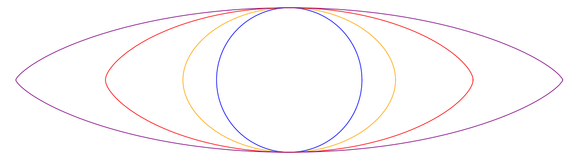
Figure 1. The Gaussian eye: the zonoids $G(c)$ for $\|c\|=0,1,2$ and $3$.

Proposition 2.9.

The map $G:c\mapsto G(c)$ is continuous. Moreover for all $c\neq 0$ the map $t\mapsto G(tc)$ is strictly increasing with respect to inclusion on $t>0.$

Proof.

To prove continuity, we use the fact that the function $h_{G(\cdot)}(\cdot):\mathbb{R}^{m}\times\mathbb{R}^{m}\to\mathbb{R}$ given by $(c,u)\mapsto h_{G(c)}(u)$ is continuous and Proposition 2.1–$(iii)$. Indeed, if $c_{n}\in\mathbb{R}^{m}$ is a sequence that converges to $c\in\mathbb{R}^{m}$, then, by continuity, we have for all $u\in\mathbb{R}^{m}$, $h_{G(c_{n})}(u)\to h_{G(c)}(u)$. In other words, $h_{G(c_{n})}$ converges pointwise to $h_{G(c)}$ and we conclude by Proposition 2.1–$(iii)$.

For the second part of the statement, we can assume without loss of generality that $\|c\|=1$. By Proposition 2.1–$(i)$, it is enough to show that given a fixed non zero point $(x,y)\in\mathbb{R}\times\mathbb{R}^{m-1}$, the function $t\mapsto h_{G(tc)}(x,y)$ is strictly increasing. We get from Proposition 2.8:

(2.8) $$\frac{\mathrm{d}}{\mathrm{d}t}h_{G(tc)}(x,y)=\frac{x}{2}\operatorname{erf}\left(\frac{tx}{\sqrt{x^{2}+\|y\|^{2}}}\right)$$

which is non–negative for all $t>0$ and positive if $x\neq 0$ and $t>0$ and this concludes the proof. ∎

We see, from Proposition 2.8, that for $c\neq 0$ the Gaussian zonoid $G(c)$ is not an ellipsoid. However we shall show in Theorem 2.10 below that it remains close to one. In order to state this result, let us first introduce a few definitions.

We define $\lambda:\mathbb{R}\to\mathbb{R}$ to be given for all $s\in\mathbb{R}$ by

(2.9) $$\lambda(s):=e^{\frac{-s^{2}}{2}}+\sqrt{\frac{\pi}{2}}s\operatorname{erf}\left(\frac{s}{\sqrt{2}}\right).$$

Note that, by Proposition 2.8 and following the same notation, for all $c\in\mathbb{R}^{m}$, we have $h_{G(c)}(1,0)=\frac{\lambda(\|c\|)}{\sqrt{2\pi}}.$ Moreover, one can see that we have $\lambda^{\prime}(s)=\sqrt{\tfrac{\pi}{2}}\operatorname{erf}\left(\tfrac{s}{\sqrt{2}}\right).$ Then we define the function $\varphi_{\infty}:\mathbb{R}^{2}\to\mathbb{R}$ given for all $(x,z)\in\mathbb{R}^{2}$ by

(2.10) $$\varphi_{\infty}(x,z):=|z|e^{\frac{-x^{2}}{\pi z^{2}}}+x\operatorname{erf}\left(\frac{x}{\sqrt{\pi}|z|}\right).$$

Theorem 2.10.

Let $c\in\mathbb{R}^{m}$ and consider the linear map $T_{c}:\mathbb{R}^{m}\to\mathbb{R}^{m}$ that is the identity if $c=0$ and that sends $c\mapsto{\lambda(\|c\|)}c$ and is the identity on $c^{\perp}$ if $c\neq 0$. Then we have

(2.11) $$b_{\infty}T_{c}\left(\frac{1}{\sqrt{2\pi}}B_{m}\right)\subset G(c)\subset T_{c}\left(\frac{1}{\sqrt{2\pi}}B_{m}\right),$$

where $B_{m}\subset\mathbb{R}^{m}$ is the unit ball and $b_{\infty}:=\min\left\{\varphi_{\infty}(\cos(t),\sin(t))\ |\ t\in[0,2\pi]\right\}\sim 0.91\ldots$

Proof.

If $c=0$, $G(0)$ is equal to the upper bound and there is nothing to prove. Thus we can assume without loss of generality that $c=se_{1}$, where $e_{1}$ is the first standard basis vector of $\mathbb{R}^{m}$ and $s>0$. Let $\widetilde{G}(s):=\sqrt{2\pi}T_{se_{1}}^{-1}G(se_{1})$. The idea of the proof is to show that the map $s\mapsto\widetilde{G}(s)$ is strictly decreasing with respect to inclusion for $s>0$. Once this is established, it is enough to show that the limit object $\widetilde{G}(\infty)$ exists and contains a ball of radius $b_{\infty}$.

Let us first show that $s\mapsto\widetilde{G}(s)$ is decreasing. For this we compute the support function $h_{\widetilde{G}(s)}(x,y)=\sqrt{2\pi}h_{G(se_{1})}\left(\frac{x}{\lambda(s)},y\right)$, where we used the same notation as in Proposition 2.8, writing $x=\langle u,e_{1}\rangle$ and $y$ for the orthogonal projection of $u$ onto $e_{1}^{\perp}.$ A straightforward computation shows that for $(x,y)\neq(0,0),$ we have:

(2.12) $$h_{\widetilde{G}(s)}(x,y)=\alpha(s)\lambda\left(\beta(s)\right),$$

where

(2.13) $$\alpha(s) :=\frac{\sqrt{x^{2}+\lambda^{2}(s)\|y\|^{2}}}{\lambda(s)}; \beta(s) :=\frac{xs}{\sqrt{x^{2}+\lambda^{2}(s)\|y\|^{2}}}.$$

Moreover, we note that $h_{\widetilde{G}(s)}(\pm x,0)=|x|$ and $h_{\widetilde{G}(s)}(0,y)=\|y\|$ do not depend on $s$. Thus we fix $x>0$ and $\|y\|\neq 0$ and omit the dependence in $(x,y)$ writing $\varphi(s):=h_{\widetilde{G}(s)}(x,y)=\alpha(s)\lambda(\beta(s)).$ It is then enough to show that $\varphi(s)$ is decreasing on $s>0$, or equivalently that $\varphi^{\prime}(s)<0$ $\forall s>0$. This requires a bit of work. First we compute $\alpha^{\prime}$ and $\beta^{\prime}$ finding:

(2.14) $$\alpha^{\prime}(s) =\frac{-x\beta(s)\lambda^{\prime}(s)}{\lambda^{2}(s)s}; \alpha(s)\beta^{\prime}(s) =\frac{x}{\lambda(s)}-\frac{\beta^{2}(s)\|y\|^{2}\lambda^{\prime}(s)}{xs}.$$

Introducing these in the expression $\varphi^{\prime}(s)=\alpha^{\prime}(s)\lambda(\beta(s))+\alpha(s)\beta^{\prime}(s)\lambda^{\prime}(\beta(s))$, we find the following.

(2.15) $$\frac{\lambda^{2}(s)s}{x\lambda^{\prime}(s)\lambda^{\prime}(\beta(s))}\varphi^{\prime}(s)=-\beta(s)\frac{\lambda(\beta(s))}{\lambda^{\prime}(\beta(s))}+s\frac{\lambda(s)}{\lambda^{\prime}(s)}-\frac{\lambda^{2}(s)\beta^{2}(s)\|y\|^{2}}{x^{2}}.$$

We will now express this in terms of yet another function:

(2.16) $$\rho(t):=t\frac{\operatorname{erf}^{\prime}(t)}{\operatorname{erf}(t)}=\sqrt{\frac{2}{\pi}}\,\frac{te^{-t^{2}}}{\operatorname{erf}(t)}.$$

We note that $t\frac{\lambda(t)}{\lambda^{\prime}(t)}=\rho\left(\frac{t}{\sqrt{2}}\right)+t^{2}$. Thus, reintroducing in (2.15) yields:

(2.17) $$\frac{\lambda^{2}(s)s}{x\lambda^{\prime}(s)\lambda^{\prime}(\beta(s))}\varphi^{\prime}(s)=\rho\left(\frac{s}{\sqrt{2}}\right)-\rho\left(\frac{\beta(s)}{\sqrt{2}}\right)+s^{2}-\beta^{2}(s)-\frac{\lambda^{2}(s)\beta^{2}(s)\|y\|^{2}}{x^{2}}.$$

It remains to see that $\beta^{2}(s)+\frac{\lambda^{2}(s)\beta^{2}(s)\|y\|^{2}}{x^{2}}=\frac{\beta^{2}(s)}{x^{2}}(x^{2}+\lambda^{2}(s)\|y\|^{2})=s^{2}$. Thus, (2.17) becomes:

(2.18) $$\frac{\lambda^{2}(s)s}{x\lambda^{\prime}(s)\lambda^{\prime}(\beta(s))}\varphi^{\prime}(s)=\rho\left(\frac{s}{\sqrt{2}}\right)-\rho\left(\frac{\beta(s)}{\sqrt{2}}\right).$$

Now, Horst Alzer shows in [Alz10, Lemma 2.1] that $\rho(t)$ is strictly decreasing for $t>0$. Moreover since $x>0$ and $y\neq 0$, we have that $\beta(s)<s$ and thus $\rho\left(\frac{\beta(s)}{\sqrt{2}}\right)>\rho\left(\frac{s}{\sqrt{2}}\right)$ for all $s>0$. Since the coefficient in front of $\varphi^{\prime}$ in (2.18) is positive for all $s>0$, this shows that $\varphi^{\prime}(s)<0$ $\forall s>0$. In definitive we have shown that for all $s>0$ the map $s\mapsto\widetilde{G}(s)$ is (strictly) decreasing with respect to inclusion.

We now proceed to study the limit as $s\to+\infty.$ For any $y\neq 0$, we have $\lim_{s\to+\infty}\alpha(s):=\|y\|$ and $\lim_{s\to+\infty}\beta(s):=\sqrt{\frac{2}{\pi}}\frac{x}{\|y\|}.$ We obtain, for any fixed $(x,y)\in\mathbb{R}\times\mathbb{R}^{m-1}$,

(2.19) $$\lim_{s\to+\infty}\varphi(s)=\varphi_{\infty}(x,\|y\|),$$

where recall the definition of $\varphi_{\infty}$ in (2.10). By Proposition 2.1–(iii), this is the support function of a convex body (zonoid) that we denote $\widetilde{G}(\infty)$ and we have $\widetilde{G}(s)\to\widetilde{G}(\infty)$ as $s\to+\infty$. By what we just proved, for all $s>0$ we have

(2.20) $$\widetilde{G}(\infty)\subset\widetilde{G}(s)\subset\widetilde{G}(0).$$

Since $T_{0}$ is the identity and by Proposition 2.7, we have that $\widetilde{G}(0)=B_{m}$. Moreover, $\widetilde{G}(\infty)$ contains a ball of radius $b_{\infty}=\min\left\{\varphi_{\infty}(\cos(t),\sin(t))\ |\ t\in[0,2\pi]\right\}=\min\left\{h_{\widetilde{G}(\infty)}(u)\ |\ \|u\|=1\right\}$. Mapping everything through $\frac{1}{\sqrt{2\pi}}T_{se_{1}}$ (which preserves inclusion) gives the result. ∎

From Theorem 2.10 and the fact that $\det(T_{c})=\lambda(\|c\|)$, we get an estimate on the volume of the Gaussian zonoids $G(c)$.

Corollary 2.11.

For every $c\in\mathbb{R}^{m}$ we have

(2.21) $$(b_{\infty})^{m}\frac{\lambda(\|c\|)}{(2\pi)^{\frac{m}{2}}}\kappa_{m}\leq\operatorname{vol}_{m}(G(c))\leq\frac{\lambda(\|c\|)}{(2\pi)^{\frac{m}{2}}}\kappa_{m},$$

where recall that $\kappa_{m}$ is the volume of the unit ball $B_{m}\subset\mathbb{R}^{m}$, $\lambda$ is defined by (2.9) and $b_{\infty}$ is defined in Theorem 2.10.

In the proof of Theorem 2.10 we proved that, for all $c\in\mathbb{R}^{m}$, $G(c)$ contains the convex body $\tfrac{1}{\sqrt{2\pi}}T_{c}(\widetilde{G}(\infty))$, see (2.20). Moreover we also proved that, as $\|c\|\to+\infty$, the renormalized convex body $(T_{c})^{-1}(G(c))$ converges to $(1/\sqrt{2\pi})\widetilde{G}(\infty)$. We can improve the lower bound on the volume of $G(c)$ and compute an asymptotic by computing the volume of $\widetilde{G}(\infty)$.

Proposition 2.12.

For all $c\in\mathbb{R}^{m}$, we have

(2.22) $$\frac{\lambda(\|c\|)}{(2\pi)^{\frac{m}{2}}}\cdot\frac{2\kappa_{m-1}}{\sqrt{m}}\leq\operatorname{vol}_{m}(G(c)).$$

Moreover, as $\|c\|\to+\infty$, we have:

(2.23) $$\lim_{\|c\|\to+\infty}\frac{1}{\|c\|}\operatorname{vol}_{m}(G(c))=\frac{1}{(2\pi)^{\frac{m-1}{2}}}\cdot\frac{\kappa_{m-1}}{\sqrt{m}}.$$

Proof.

We are going to show that

(2.24) $$vol_{m}(\widetilde{G}(\infty))=2\kappa_{m-1}/\sqrt{m}.$$

Then the first statement follows from the fact that $G(c)$ contains $\tfrac{1}{\sqrt{2\pi}}T_{c}(\widetilde{G}(\infty))$.

Recall that the support function of $\widetilde{G}(\infty)$ is given by $h_{\widetilde{G}(\infty)}(x,y)=\varphi_{\infty}(x,\|y\|)$, where $\varphi_{\infty}$ is defined in (2.10). We compute its gradient and find for $\|y\|\neq 0$: $\frac{\partial}{\partial x}h_{\widetilde{G}(\infty)}(x,y)=\operatorname{erf}\left(\frac{x}{\sqrt{\pi}\|y\|}\right)$ and $\frac{\partial}{\partial y_{i}}h_{\widetilde{G}(\infty)}(x,y)=\frac{y_{i}}{\|y\|}\exp\left(\frac{-x^{2}}{\pi\|y\|^{2}}\right)$

Thus, by Proposition 2.1-$(iv)$, the boundary of $\widetilde{G}(\infty)$ is described by the equation $\|y\|=f(x)$ with $f(x):=\exp\left(-(\operatorname{erf}^{-1}(x))^{2}\right)$ and $x\in[-1,1]$. Hence its volume is given by

(2.25) $$\operatorname{vol}_{m}(\widetilde{G}(\infty))=\int_{-1}^{1}\kappa_{m-1}f(x)^{m-1}\mathrm{d}x.$$

We apply the change of variable $x=\operatorname{erf}(u)$ to find

(2.26) $$\operatorname{vol}_{m}(\widetilde{G}(\infty))=\kappa_{m-1}\frac{2}{\sqrt{\pi}}\int_{-\infty}^{\infty}e^{-mu^{2}}\mathrm{d}u.$$

Changing variables again with $u=s/\sqrt{2m}$ gives (2.24) and thus the firt part of the statement.

To prove the limit, we notice first that, since $(T_{c})^{-1}(G(c))$ converges to $(1/\sqrt{2\pi})\widetilde{G}(\infty)$ as $\|c\|\to+\infty$, we get that

(2.27) $$\lim_{\|c\|\to+\infty}\frac{1}{\lambda(\|c\|)}\operatorname{vol}_{m}(G(c))=\frac{1}{(2\pi)^{\frac{m}{2}}}\cdot\frac{2\kappa_{m-1}}{\sqrt{m}}.$$

Then it is enough to note that $\lim_{s\to+\infty}\frac{\lambda(s)}{s}=\sqrt{\frac{\pi}{2}}$. ∎

3. Application to random determinants

Richard Vitale shows in [Vit91] that if $M\in\mathbb{R}^{m\times m}$ is a random matrix with iid columns distributed as some integrable random vector $X\in\mathbb{R}^{m}$, then $\mathbb{E}|\det(M)|=m!\operatorname{vol}_{m}(\mathbb{E}\underline{X})$ (recall the definition of $\mathbb{E}\underline{X}$ in (2.2)). In  [BBLM21, Section 5] this is generalized to a larger class of random determinants, where the columns are not necessarily identically distributed. We state below the case of a rectangular matrix with independent columns which is a particular case of [BBLM21, Theorem 5.4] reformulated in a language more suitable for our context.

Lemma 3.1.

Let $0<k\leq m$ and let $X_{1},\ldots,X_{k}\in\mathbb{R}^{m}$ be independent integrable random vectors. Consider the random matrix $\Gamma:=\left(X_{1},\ldots,X_{k}\right)\in\mathbb{R}^{m\times k}$ whose columns are the vectors $X_{i}$ and let $K_{i}:=\mathbb{E}\underline{X_{i}}$ be the zonoid defined in (2.2). Then we have

(3.1) $$\mathbb{E}\sqrt{\det(\Gamma^{t}\Gamma)}=\frac{m!}{(m-k)!\kappa_{m-k}}\operatorname{V}(K_{1},\ldots,K_{k},B_{m}[m-k]),$$

where $B_{m}[m-k]$ denotes the unit ball $B_{m}\subset\mathbb{R}^{m}$ repeated $m-k$ times in the argument and where recall that $\kappa_{m-k}=\operatorname{vol}_{m-k}(B_{m-k})$.

Proof.

First note that $\sqrt{\det\left(\Gamma^{t}\Gamma\right)}$ is equal to the $k$–th dimensional volume of the parallelotope spanned by the vectors $X_{1},\ldots,X_{k}$, i.e. to the volume of the Minkowski sum $[0,X_{1}]+\cdots+[0,X_{k}]$. Writing $\underline{X}$ to denote the segment $\frac{1}{2}[-X,X]$ (which is a translate of the segment $[0,X]$), we have that $\sqrt{\det\left(\Gamma^{t}\Gamma\right)}$ is equal to the $k$–th dimensional volume of $\underline{X_{1}}+\cdots+\underline{X_{k}}$. Using Proposition 2.2-$(iii)$, we obtain

(3.2) $$\sqrt{\det\left(\Gamma^{t}\Gamma\right)}=\frac{\binom{m}{k}}{\kappa_{m-k}}\operatorname{V}(\underline{X_{1}}+\cdots+\underline{X_{k}}[k],B_{m}[m-k])=\frac{m!}{(m-k)!\kappa_{m-k}}\operatorname{V}(\underline{X_{1}},\ldots,\underline{X_{k}},B_{m}[m-k]),$$

where the second equality is obtained by expanding by multilinearity the mixed volume (Proposition 2.2-$(ii)$) and eliminating every term where a segment appear twice by Proposition 2.2-$(iv)$. Finally by [BBLM21, Theorem 5.4] we obtain, taking the expectation:

(3.3) $$\mathbb{E}\operatorname{V}(\underline{X_{1}},\ldots,\underline{X_{k}},B_{m}[m-k])=\operatorname{V}(K_{1},\ldots,K_{k},B_{m}[m-k]),$$

which concludes the proof. ∎

In the case where $X_{i}$ is a (non–degenerate) Gaussian vector, the zonoid $K_{i}$ is, by definition, a Gaussian zonoid and thus is a linear image of some $G(c_{i})$ (see the previous section). Since the mixed volume is increasing with respect to inclusion (Proposition 2.2-$(v)$), Lemma 3.1 and Theorem 2.10 imply the following.

Theorem 3.2.

Let $0<k\leq m$ and let $X_{1},\ldots,X_{k}\in\mathbb{R}^{m}$ be independent Gaussian vectors such that $X_{i}=M_{i}(c_{i}+\xi_{i})$ with $M_{i}:\mathbb{R}^{m}\to\mathbb{R}^{m}$ an invertible linear map, $c_{i}\in\mathbb{R}^{m}$ fixed vectors and $\xi_{i}\in\mathbb{R}^{m}$ iid standard Gaussian vectors. Consider the random matrix $\Gamma:=(X_{1},\ldots,X_{k})$ whose columns are the vectors $X_{i}$ and define the ellipsoids $\mathcal{E}_{i}:=M_{i}\circ T_{c_{i}}\left(B_{m}\right)$ for $i=1,\ldots,k$, where recall the definition of $T_{c}$ in Theorem 2.10. We have

(3.4) $$(b_{\infty})^{k}\alpha_{m,k}\operatorname{V}\left(\mathcal{E}_{1},\ldots,\mathcal{E}_{k},B_{m}[m-k]\right)\leq\mathbb{E}\sqrt{\det\left(\Gamma^{t}\Gamma\right)}\leq\alpha_{m,k}\operatorname{V}\left(\mathcal{E}_{1},\ldots,\mathcal{E}_{k},B_{m}[m-k]\right),$$

where $B_{m}[m-k]$ denotes the unit ball $B_{m}\subset\mathbb{R}^{m}$ repeated $m-k$ times in the argument of the mixed volume $\operatorname{V}$, $\alpha_{m,k}:=\frac{m!}{(2\pi)^{k/2}(m-k)!\kappa_{m-k}}$ and $b_{\infty}$ is defined in Theorem 2.10.

This result is to be compared with [KZ12, Theorem 1.1] where it is proved that the centered case (i.e. when all the $c_{i}$ are equal to $0$) is equal to the mixed volume of ellipsoids, that is to the upper bound. More precisely, if $Y_{i}$ is a centered Gaussian vector with covariance matrix $\Sigma_{i}:=M_{i}T_{c_{i}}T_{c_{i}}^{t}M_{i}^{t},$ and $Y_{1},\ldots,Y_{k}$ are independent and if $\widetilde{\Gamma}:=(Y_{1},\ldots,Y_{k})$, then by [KZ12, Theorem 1.1] we have $\mathbb{E}\sqrt{\det\left(\widetilde{\Gamma}^{t}\widetilde{\Gamma}\right)}=\alpha_{m,k}\operatorname{V}\left(\mathcal{E}_{1},\ldots,\mathcal{E}_{k},B_{m}[m-k]\right).$ One can interpret Theorem 3.2 by saying that, for random determinants, the non–centered Gaussian vector $X_{i}$ is "trapped" between the centered Gaussian vectors $b_{\infty}Y_{i}$ and $Y_{i}$. Note that in that case we also have $\mathbb{E}\underline{Y_{i}}=\tfrac{1}{\sqrt{2\pi}}\mathcal{E}_{i}$ and thus Lemma 3.1 gives an alternative proof of [KZ12, Theorem 1.1].

Remark 3.3.

Lemma 3.1 is still valid if the random vectors are degenerate (i.e almost surely contained in an hyperplane). Hence, Theorem 3.2 is still valid if the map $M_{i}$ is not surjective. However one cannot obtain all degenerate Gaussian vectors this way as this does not cover the case where the support is contained in an affine hyperplane.

If $k=m$ and all the Gaussian vectors are identically distributed we obtain the following.

Proposition 3.4.

Let $\xi_{1},\ldots,\xi_{m}\in\mathbb{R}^{m}$ be iid standard Gaussian vectors, let $M:\mathbb{R}^{m}\to\mathbb{R}^{m}$ be an invertible linear map, $c\in\mathbb{R}^{m}$ a fixed vector and define the iid Gaussian vectors $X_{i}:=M(c+\xi_{i})$ for $i=1,\ldots,m$. Consider the random square matrix $\Gamma:=(X_{1},\ldots,X_{m})$ whose columns are the vectors $X_{i}$. We have

(3.5) $$|\det M|\frac{\lambda(\|c\|)}{(2\pi)^{\frac{m}{2}}}\frac{2m!\kappa_{m-1}}{\sqrt{m}}\leq\mathbb{E}|\det\Gamma|\leq|\det M|\frac{\lambda(\|c\|)}{(2\pi)^{\frac{m}{2}}}m!\kappa_{m}.$$

Moreover, as $\|c\|\to+\infty$, we have:

(3.6) $$\lim_{\|c\|\to+\infty}\frac{1}{\|c\|}\mathbb{E}|\det\Gamma|=|\det M|\frac{1}{(2\pi)^{\frac{m-1}{2}}}\cdot\frac{m!\kappa_{m-1}}{\sqrt{m}}.$$

Proof.

By Lemma 3.1, we have that $\mathbb{E}|\det\Gamma|=m!\operatorname{vol}_{m}(M(G(c)))=m!|\det M|\operatorname{vol}_{m}(G(c))$. Then the upper boud follows from Corollary 2.11, and the lower bound and the limit follow from Proposition 2.12. ∎

Remark 3.5.

Note that the Gaussian vectors $X_{i}=M(\xi_{i}+c)$ have covariance matrix $MM^{t}$ and thus $|\det M|=\sqrt{\det(MM^{t})}$ is a function of this covariance matrix.

4. Gaussian perturbation of a hypersurface

In [MS22], Michele Stecconi and the author, studied the zero set of random fields, i.e. random functions on a Riemannian manifold. They identify a class of random fields for which their theory apply that they call zKROK fields, see [MS22, Definition 4.1].

Let $M$ be a Riemannian manifold of dimension $m$. For a zKROK field $X\in C^{1}(M)$ there is a notion of conditioning to the event $\left\{X(p)=0\right\}$ for any $p\in M$. In particular one can consider the random vector

(4.1) $$(\mathrm{d}_{p}X|X(p)=0)\in T^{*}_{p}M.$$

This vector corresponds to a normal vector at $p$ to the random submanifold $X^{-1}(0)$ conditionned to the fact that $p\in X^{-1}(0)$, see [MS22, Section 4.1] for a more rigorous definition and details.

Remark 4.1.

If $X:M\to\mathbb{R}$ is zKROK and such that for all $p\in M$ we have that $X(p)$ is independent of $\mathrm{d}_{p}X$ then $(\mathrm{d}_{p}X|X(p)=0)$ has the same law as $\mathrm{d}_{p}X$. Indeed it is enough to see that this satisfies the definition of the regular conditional probability, see [MS22, (4.1)].

Using this random vector, one associates to a zKROK field a family of zonoids in the cotangent space, see [MS22, Definition 5.1].

Definition 4.2.

Let $X:M\to\mathbb{R}$ be a zKROK field. For all $p\in M$, we define the following zonoid in $T^{*}_{p}M$:

(4.2) $$\zeta_{X}(p):=\rho_{X(p)}(0)\mathbb{E}\left[\underline{\mathrm{d}_{p}X}|X(p)=0\right],$$

where $\rho_{X(p)}(0)$ denotes the density of the random variable $X(p)\in\mathbb{R}$ at $0$ and $\mathbb{E}\left[\underline{\mathrm{d}_{p}X}|X(p)=0\right]$ is the Vitale zonoid associated to the random vector $(\mathrm{d}_{p}X|X(p)=0)$ from (4.1). We call $\zeta_{X}$ the zonoid section associated to the random field $X$.

Remark 4.3.

The zonoid section defined in [MS22, Definition 5.1] is slightly different than Definition 4.2. Indeed, the zonoid section defined by Definition 4.2, is called the centered zonoid section in [MS22] and is denoted by $\underline{\zeta_{X}}$. It is a translate of what they call the zonoid section. Since we only consider translation invariant quantities such as volume or mixed volume, this makes no difference.

The main result of [MS22] is that these zonoids compute the expected volume of the zero set of the zKROK fields and behave well under independent intersection. In our context of scalar fields, we will use the following special case, which is [MS22, Corollary 7.2].

Proposition 4.4.

Let $M$ be a Riemannian manifold of dimension $m$, let $X_{1},\ldots,X_{m}:M\to\mathbb{R}$ be independent zKROK fields and let $Z_{i}:=X_{i}^{-1}(0)$, $i=1,\ldots,m$. We have, for all $U\subset M$ open:

(4.3) $$\mathbb{E}\#(Z_{1}\cap\cdots\cap Z_{m}\cap U)=m!\int_{U}\operatorname{V}(\zeta_{X_{1}}(p),\ldots,\zeta_{X_{m}}(p))\,\mathrm{d}M(p),$$

where $\mathrm{d}M(p)$ denotes the integration with respect to the volume form on $M$ and $\operatorname{V}$ is the mixed volume (see beginning of Section 3).

A particular case of random fields are the Gaussian Random Field (GRF). A GRF on $M$ is a random function $X$, such that for all finite collection of points $p_{1},\ldots,p_{k}\in M$, the random vector $(X(p_{1}),\ldots,X(p_{k}))\in\mathbb{R}^{k}$ is a Gaussian vector. In the following, we will only consider GRF that are smooth almost surely. We will show how the Gaussian zonoids appear in this context.

One can show that all non–degenerate GRF are zKROK. More precisely, we have (see [MS22, Proposition 4.9.]) that a GRF $X\in C^{\infty}(M)$ is zKROK if for all $p\in M$, the Gaussian variable $X(p)$ is non–degenerate.

If $X(p)$ is a standard Gaussian variable for all $p\in M$ we say that $X$ is a standard GRF. Equivalentely, a GRF $X$ is standard if and only if for all $p\in M$, $\mathbb{E}[X(p)]=0$ and $\mathbb{E}[X(p)^{2}]=1$.

Remark 4.5.

Note that in that case, by differentiating the equation $\mathbb{E}[X(p)^{2}]=1$, we get for all $p\in M$, that $\mathbb{E}\left[X(p)\mathrm{d}_{p}X\right]=0$, i.e. $X(p)$ is independant of $\mathrm{d}_{p}X$.

The link between the geometry of a Riemannian manifold and GRF is studied by Robert Adler and Jonathan Taylor in [AT09]. In particular, we have that for every Riemannian manifold $(M,\langle\cdot,\cdot\rangle)$ there is a standard GRF $g\in C^{\infty}(M)$ such that the Riemannian metric is given by the covariance matrix of $g$. More precisely, such that for all $v,w\in T_{p}M$

(4.4) $$\langle v,w\rangle=\mathbb{E}\left[\mathrm{d}_{p}g(v)\cdot\mathrm{d}_{p}g(w)\right].$$

For more details, see [AT09, Section 10.2], for another extensive study of GRF the reader can also refer to [LS19].

Remark 4.6.

If $g\in C^{\infty}(M)$ is a standard GRF satisfying (4.4), then $\mathrm{d}_{p}g\in T^{*}_{p}M$ is a standard Gaussian vector for the Riemannian metric. Thus, it follows from Definition 4.2, that the associated zonoid section is $\zeta_{g}(p)=\tfrac{1}{2\pi}B_{M}(p)$, where $B_{M}(p)$ is the unit ball in $T^{*}_{p}M$ for the Riemannian metric.

We now come to our main object of study for this section: non–centered GRF.

Definition 4.7.

Let $g\in C^{\infty}(M)$ be a standard GRF satisfying (4.4). Let $\varphi\in C^{\infty}(M)$ be a fixed function and let $\tau\geq 0$. We define the following random field.

(4.5) $$X_{\tau}:=\varphi+\tau g.$$

Moreover, we write $Z_{\tau}:=X_{\tau}^{-1}(0)$.

We can compute the zonoid section explicitely in terms of Gaussian zonoids.

Proposition 4.8.

For all $\tau>0$, the random field $X_{\tau}$ is zKROK and its zonoid section is given for all $p\in M$ by

(4.6) $$\zeta_{\tau}(p):=\zeta_{X_{\tau}}(p)=\frac{e^{\frac{-\varphi(p)^{2}}{2\tau^{2}}}}{\sqrt{2\pi}}G\left(\frac{\mathrm{d}_{p}\varphi}{\tau}\right).$$

Proof.

For all $p\in M$, we have that $X_{\tau}(p)\in\mathbb{R}$ is a Gaussian variable or mean $\varphi(p)$ and variance $\tau^{2}$. Thus $X_{\tau}$ is zKROK and for all $p\in M$ the density at $0$ of $X_{\tau}(p)$ is given by:

(4.7) $$\rho_{X_{\tau}(p)}(0)=\frac{e^{\frac{-\varphi(p)^{2}}{2\tau^{2}}}}{\sqrt{2\pi}\tau}.$$

Moreover, since $g(p)$ is independent of $\mathrm{d}_{p}g$ (see Remark 4.5), we have that $X_{\tau}(p)=\varphi(p)+\tau g(p)$ is also independent of $\mathrm{d}_{p}X_{\tau}=\mathrm{d}_{p}\varphi+\tau\mathrm{d}_{p}g$. Thus, by Remark 4.1, we obtain

(4.8) $$\mathbb{E}\left[\underline{\mathrm{d}_{p}X_{\tau}}|X_{\tau}(p)=0\right]=\mathbb{E}\underline{\mathrm{d}_{p}X_{\tau}}=\mathbb{E}\underline{\mathrm{d}_{p}\varphi+\tau\mathrm{d}_{p}g}=\tau\cdot G\left(\frac{\mathrm{d}_{p}\varphi}{\tau}\right),$$

where, in the last equality, we used the fact that $\mathrm{d}_{p}g$ is a standard Gaussian vector in $T^{*}_{p}M$ (with the Riemannian metric). The result then follows by multiplying (4.8) by (4.7). ∎

These zonoids satisfy the following obvious properties.

Proposition 4.9.

The zonoid section $\zeta_{\tau}$ satisfy the following properties.

1. For all $p\in M$, we have:

   (4.9) $$\zeta_{\tau}(p)\xrightarrow[\tau\to\infty]{}\frac{1}{2\pi}B_{M}(p),$$

   where $B_{M}(p)\subset T^{*}_{p}M$ is the unit ball.

2. For all $p\in M\setminus Z_{0}$ we have:

   (4.10) $$\zeta_{\tau}(p)\xrightarrow[\tau\to 0]{}\{0\}.$$

3. Let $p\in Z_{0}$, and let $\pi_{p}:T^{*}_{p}M\to T^{*}_{p}Z_{0}$ be the orthogonal projection. For all $\tau>0$, we have:

   (4.11) $$\pi_{p}(\zeta_{\tau}(p))=\frac{1}{2\pi}B_{Z_{0}}(p),$$

   where $B_{Z_{0}}(p)\subset T^{*}_{p}Z_{0}$ is the unit ball for the Riemannian metric on $Z_{0}$ induced from $M$.

These properties have a geometric interpretation. Indeed the zonoid section $\zeta_{\tau}$ corresponds to a Finsler structure on $M$, i.e. a norm on each tanget space, given by the support function of the zonoids $\zeta_{\tau}(p)$, see [MS22, Section 9]. For each $\tau>0$ we then have a Finsler geometry on $M$. Property $(1)$ says that when $\tau$ is large this geometry tends to the Riemannian geometry that we started with. Propery $(2)$ says that, when $\tau$ is small, everything outside $Z_{0}$ disappears, i.e. the Finsler geometry shrinks around $Z_{0}$ as $\tau$ goes to zero. Finally property $(3)$ says that, for all $\tau>0$, this Finsler geometry restricted to $Z_{0}$ gives the Riemannian geometry of $Z_{0}$ (in particular it is independent of $\tau$).

Centered and standard GRF are more extensively studied and often easier to deal with. We show that, in our case, we can estimate the GRF $X_{\tau}$ by some standard GRF.

Theorem 4.10.

For every $\tau>0$, there is a standard GRF $\widetilde{X}_{\tau}$ such that for every zKROK fields $Y_{1},\ldots,Y_{m-1}\in C^{1}(M)$ independents and independents of $X_{\tau},\widetilde{X}_{\tau}$, writing $\widetilde{Z}_{\tau}:=\widetilde{X}_{\tau}^{-1}(0)$ and $W:=Y_{1}^{-1}(0)\cap\cdots\cap Y_{m-2}^{-1}(0)$, we have, for every open set $U\subset M$:

(4.12) $$b_{\infty}\cdot\mathbb{E}\#\left(\widetilde{Z}_{\tau}\cap W\cap U\right)\leq\mathbb{E}\#\left(Z_{\tau}\cap W\cap U\right)\leq\mathbb{E}\#\left(\widetilde{Z}_{\tau}\cap W\cap U\right),$$

where recall the definition of $b_{\infty}$ in Theorem 2.10.

Proof.

By Theorem 2.10, for every $p\in M$, we have that:

(4.13) $$\frac{b_{\infty}}{2\pi}\mathcal{E}_{\tau}(p)\subset\zeta_{\tau}(p)\subset\frac{1}{2\pi}\mathcal{E}_{\tau}(p),$$

where $\mathcal{E}_{\tau}(p)=e^{\frac{-\varphi(p)^{2}}{2\tau^{2}}}T_{c}B_{p}$ with $c=\mathrm{d}_{p}\varphi/\tau\in T^{*}_{p}M$ and where recall the definition of the linear map $T_{c}$ in Theorem 2.10. Now the ellipsoid $\mathcal{E}_{\tau}(p)$ defines a Riemannian metric on $M$ for every $\tau>0$ and thus there is a standard GRF $\widetilde{X}_{\tau}$ that satisfies (4.4) for this metric. In that case, by Remark 4.6, we have that the associated zonoid section is precisely $\zeta_{\widetilde{X}_{\tau}}(p)=\frac{1}{2\pi}\mathcal{E}_{\tau}(p)$ for every $p\in M$. The result then follows from Proposition 4.4 and monotonicity of the mixed volume. ∎

It is not difficult to see that the ellipsoid section $\frac{1}{2\pi}\mathcal{E}_{\tau}$ and the Riemannian metric that it defines also satisfy the properties of Proposition 4.9.

Remark 4.11.

A more refined analysis of [MS22] (more precisely, using [MS22, (7.2)]), shows that the assumption that the random fields $Y_{1},\ldots,Y_{m-1}$ are independent is not needed and one only needs that the random field $(Y_{1},\ldots,Y_{m-1}):M\to\mathbb{R}^{m-1}$ is zKROK. Nevertheless, one still needs to assume that this field is independent of $X_{\tau}$ and $\widetilde{X}_{\tau}$. To formulate and prove this would require to introduce zonoid calculus and the wedge product of zonoid which we chose not to do here for simplicity.

We conclude this section by an asymptotic analysis for small $\tau$. As $\tau\to 0$, we expect that the random zero set $Z_{\tau}$ concentrates around $Z_{0}$. In fact, Proposition 4.9-$(2)$ shows that this is the case. We can nevertheless study this concentration more precisely and quantitatively.

For all $r>0$ we define the following open neighbourhood of $Z_{0}$:

(4.14) $$\mathcal{U}_{r}:=\left\{p\in M\ |\ |\varphi(p)|<r\right\}\subset M.$$

Moreover, for all $\tau,r>0$ we let

(4.15) $$n_{r,\tau}:=\mathbb{E}\#\left(Z^{(1)}_{\tau}\cap\cdots\cap Z^{(m)}_{\tau}\cap\mathcal{U}_{r}\right),$$

where $Z^{(1)}_{\tau},\ldots,Z^{(m)}_{\tau}$ are iid copies of $Z_{\tau}=X_{\tau}^{-1}(0)$.

Theorem 4.12.

Assume that $M$ is a compact manifold of dimension $m$ and that $0$ is a regular value of $\varphi$. Let $r=r(\tau)$ be such that $\lim_{\tau\to 0}r=0$ and $\alpha:=\lim_{\tau\to 0}\tfrac{r}{\tau}\in[0,+\infty]$ exists. Then we have:

(4.16) $$\lim_{\tau\to 0}n_{r,\tau}=\frac{(m-1)!\kappa_{m-1}}{(2\pi)^{m-1}}\cdot\operatorname{erf}\left(\sqrt{\frac{m}{2}}\cdot\alpha\right)\cdot\operatorname{vol}_{m-1}(Z_{0}).$$

Proof.

By Proposition 4.4, we have

(4.17) $$n_{r,\tau}=m!\int_{\mathcal{U}_{r}}\operatorname{vol}_{m}(\zeta_{\tau}(p))\mathrm{d}M(p)=\frac{m!}{(2\pi)^{\frac{m}{2}}}\int_{\mathcal{U}_{r}}e^{\frac{-m\varphi(p)^{2}}{2\tau^{2}}}\operatorname{vol}_{m}\left(G\left(\frac{\mathrm{d}_{p}\varphi}{\tau}\right)\right)\mathrm{d}M(p).$$

Since $0$ is a regular value of $\varphi$, for $\tau$ small enough, there is no critical point of $\varphi$ in $\mathcal{U}_{r}$. Thus we can apply the smooth coarea formula to the function $\varphi:\mathcal{U}_{r}\to(-r,r)$ to get:

(4.18) $$n_{r,\tau}=\frac{m!}{(2\pi)^{\frac{m}{2}}}\int_{-r}^{r}e^{\frac{-mt^{2}}{2\tau^{2}}}\int_{S_{t}}\frac{1}{\|\mathrm{d}_{p}\varphi\|}\operatorname{vol}_{m}\left(G\left(\frac{\mathrm{d}_{p}\varphi}{\tau}\right)\right)\mathrm{d}S_{t}(p)\mathrm{d}t,$$

where $S_{t}:=\varphi^{-1}(t)$. Now we apply the change of variable $u=\frac{\sqrt{m}}{\sqrt{2}\tau}t$ to obtain:

(4.19) $$n_{r,\tau}=\frac{m!}{(2\pi)^{\frac{m}{2}}}\sqrt{\frac{2}{m}}\int_{-\sqrt{\frac{m}{2}}\cdot\frac{r}{\tau}}^{\sqrt{\frac{m}{2}}\cdot\frac{r}{\tau}}e^{-u^{2}}\int_{S_{t(u)}}\frac{\tau}{\|\mathrm{d}_{p}\varphi\|}\operatorname{vol}_{m}\left(G\left(\frac{\mathrm{d}_{p}\varphi}{\tau}\right)\right)\mathrm{d}S_{t(u)}(p)\mathrm{d}u,$$

where $t(u)=\sqrt{\frac{2}{m}}\cdot\tau u$. We have that $t(u)\in[-r,r]$ and thus $t(u)\to 0$ uniformly in $u$ as $\tau\to 0$. Moreover, by Proposition 2.12, we have $\frac{\tau}{\|\mathrm{d}_{p}\varphi\|}\operatorname{vol}_{m}\left(G\left(\frac{\mathrm{d}_{p}\varphi}{\tau}\right)\right)\xrightarrow[\tau\to 0]{}\frac{\kappa_{m-1}}{\sqrt{m}(2\pi)^{\frac{m-1}{2}}}.$ By compactness, this is also uniform in $p$. We obtain that, as $\tau\to 0$, we have

(4.20) $$n_{r,\tau}\to\frac{(m-1)!}{(2\pi)^{m}}\sqrt{2\pi}\kappa_{m-1}\sqrt{2}\cdot 2\int_{0}^{\sqrt{\frac{m}{2}}\alpha}e^{-u^{2}}\mathrm{d}u\,\operatorname{vol}_{m-1}(S_{0}).$$

The result then follows by noting that $S_{0}=Z_{0}$ and by recognizing the error function.

∎

References

• [Alz10] Horst Alzer. Error function inequalities. Advances in Computational Mathematics, 33:349–379, 10 2010.
• [AT09] Robert J. Adler and Jonathan E. Taylor. Random Fields and Geometry. Springer Monographs in Mathematics. Springer New York, 2009.
• [BBLM21] Paul Breiding, Peter Bürgisser, Antonio Lerario, and Léo Mathis. The zonoid algebra, generalized mixed volumes, and random determinants, 2021.
• [KZ12] Zakhar Kabluchko and Dmitry Zaporozhets. Random determinants, mixed volumes of ellipsoids, and zeros of gaussian random fields. Journal of Mathematical Sciences, 199, 06 2012.
• [LNN61] F. C. Leone, L. S. Nelson, and R. B. Nottingham. The folded normal distribution. Technometrics, 3(4):543–550, 1961.
• [LS19] Antonio Lerario and Michele Stecconi. Differential topology of gaussian random fields, 2019.
• [Mat22] Léo Mathis. The handbook of zonoid calculus. PhD thesis, Scuola Internazionale di Studi Avanzati, 2022.
• [MN21] Ilya Molchanov and Felix Nagel. Diagonal minkowski classes, zonoid equivalence, and stable laws. Communications in Contemporary Mathematics, 23(02):1950091, 2021.
• [Mol06] I. Molchanov. Theory of Random Sets. Probability and Its Applications. Springer London, 2006.
• [Mos02] Karl Mosler. Multivariate dispersion, central regions and depth. The lift zonoid approach, volume 165. 01 2002.
• [MS22] Léo Mathis and Michele Stecconi. Density of a random submanifold: the zonoid section, 2022.
• [MT21] Ilya Molchanov and Riccardo Turin. Convex bodies generated by sublinear expectations of random vectors. Advances in Applied Mathematics, 131:102251, 2021.
• [Sch14] Rolf Schneider. Convex bodies: the Brunn-Minkowski theory, volume 151 of Encyclopedia of Mathematics and its Applications. Cambridge University Press, Cambridge, expanded edition, 2014.
• [Sch22] Rolf Schneider. Random zonotopes and valuations, 2022.
• [Vit91] Richard A. Vitale. Expected absolute random determinants and zonoids. Ann. Appl. Probab., 1(2):293–300, 1991.
• [Wik22] Wikipedia contributors. Folded normal distribution — Wikipedia, the free encyclopedia, 2022. [Online; accessed 18-January-2022].