On the sample complexity of stabilizing linear dynamical systems from data

Abstract

Learning controllers from data for stabilizing dynamical systems typically follows a two step process of first identifying a model and then constructing a controller based on the identified model. However, learning models means identifying generic descriptions of the dynamics of systems, which can require large amounts of data and extracting information that are unnecessary for the specific task of stabilization. The contribution of this work is to show that if a linear dynamical system has dimension (McMillan degree) $n$, then there always exist $n$ states from which a stabilizing feedback controller can be constructed, independent of the dimension of the representation of the observed states and the number of inputs. By building on previous work, this finding implies that any linear dynamical system can be stabilized from fewer observed states than the minimal number of states required for learning a model of the dynamics. The theoretical findings are demonstrated with numerical experiments that show the stabilization of the flow behind a cylinder from less data than necessary for learning a model.

1 Introduction

Learning feedback controllers from data for stabilizing dynamical systems typically follows a two step process: First, a model of the underlying system of interest is identified from data. Then, a controller is constructed based on the identified model [17]. However, learning models means identifying generic descriptions of the dynamics of systems, which can require large amounts of data and can include extracting information about the systems that are unnecessary for the specific task of finding stabilizing controllers. Additionally, if data are received in form of observed state trajectories, then they can come in non-minimal representations in spaces of higher dimensions than the minimal dimension of the space in which the dynamics of the systems evolve; cf. McMillan degree [1, Sec. 4.2.2]. The non-minimal representation of the observed states means that higher dimensional models are learned than necessary for describing the system, which in turn requires even larger numbers of samples and higher training costs.

This work focuses on the design of low-dimensional state-feedback controllers for linear dynamical systems. The main finding is that even if states of a system are observed in a high-dimensional representation, the required number of states to learn a stabilizing controller scales with the intrinsic, minimal dimension of the system rather than the dimension of the representation of the states: If a system has dimension $n$, then there exist $n$ states from which a stabilizing feedback controller can be constructed (Corollary 3 on page 3). If instead only $n-1$ or fewer states are observed, then there cannot exist a feedback controller that stabilizes all systems from which the sampled states can be observed. This finding shows that stabilization via state-feedback can be achieved from fewer observed states than the minimal number of states required for identifying models, which is a consequence of [56] and means that the stabilization of any linear dynamical system, for which a stabilizing controller exists, is possible with less data than learning a model.

The task of data-driven controller design roots back to [60], which led to model-free controller design in which controllers are learned via the parametrization of suitable control laws that are tuned via optimization against given data; see, for example, [19, 26, 38, 47]. The development of model reduction techniques [1, 7, 10, 11, 45] made model-based control tractable, which allows the application of more complex control laws than in controller tuning. In particular, model reduction also motivated the two step approach of first system identification and subsequent controller design because reduced models are of lower dimensions and thus cheaper to identify; even though it is far from guaranteed that controllers based on identified reduced models stabilize the original system. A large body of work has been established for learning (reduced) dynamical-system models from data such as dynamic mode decomposition and operator inference [50, 53, 44, 42], sparse identification methods [18, 49, 48], and the Loewner framework [4, 39, 43, 52, 51]. All of these methods are aiming to identify general models rather than learning models specifically for the purpose of controller design. In [33, 34], the authors take into account the task of control when learning models and focus on nonlinear systems. However, no sample complexity results are provided. In [16], the authors select data such that they are informative for control with models learned via the Koopman operator, and in the work [35] models are constructed adaptively from data for controlling systems with quickly changing dynamics. The authors of [23, 54] balance model approximation error and control but aim to identify models of the same dimension as the observed states, rather than learning low-dimensional controllers as in the present work.

The construction of low-dimensional controllers has been studied extensively by the model reduction community; see, e.g., [6, 8, 9, 15, 32]. Such classical techniques belong to the class of approaches consisting of two steps of first, identifying a general (reduced) model of the system from data, followed by the controller design. The authors of [25, 29] show that several of the classical model reduction methods such as balanced and modal truncation are applicable even if only data are available; however, it remains unclear how many data samples are necessary to learn the reduced models and subsequently construct stabilizing controllers.

The idea of data-driven controller construction regained anew interest through the influential work [59]. It introduced the so-called fundamental lemma of linear systems that states that all trajectories of a linear system can be obtained from any given trajectory under the assumption that the input signal is persistently exciting. This result can be applied to study system identification, but it also led to new approaches and strategies for controller design such as the data-driven construction of stabilizing state-feedback controllers [14, 56, 22]. This line of work serves as a building block for our contribution. We build on [56], which shows that fewer data samples are sufficient for stabilization than for identifying models in certain situations; however, the work [56] does not consider low-dimensional representations and operates in spaces that have the same dimension as the observed states. In contrast, we show that the intrinsic, minimal dimension of a system determines how many states need to be observed for stabilization, independent of the dimension of the data. Key to the analysis is a combination of arguments common in model reduction [1] with a careful distinction between the stabilizability of systems versus the stabilizability of models of systems. The distinction between model and system is particularly important for data-driven control because models learned from non-minimal representations of data are not unique and thus can be unstabilizable, which makes stabilization via the identified models intractable independent of whether the underlying systems are stabilizable or not.

The manuscript is organized as follows: Preliminaries and building blocks for this work are described in Section 2. We will carefully distinguish between models of systems and the systems themselves. The main contribution is Section 3 that shows that the number of observed states required for stabilization scales with the dimension of the system rather than the dimension of the data and the model. The case of approximately low-dimensional systems is discussed, too. In Section 4, we provide computational algorithms. Numerical examples in Section 5 demonstrate the theory and conclusions are drawn in Section 6.

2 Preliminaries

This section reviews classical results about system identification for linear dynamical systems and discusses the concept of data informativity that was introduced in [27, 56].

2.1 Sampling data from dynamical systems

We consider data triplets of the form $(U_{-},X_{-},X_{+})$. If the system from which data are sampled is discrete in time, then state-space models have the form

$$x(t+1) =Ax(t)+Bu(t),\qquad t\in\mathbb{N}_{0},$$ (1)

with $A\in\mathbb{R}^{N\times N}$ and $B\in\mathbb{R}^{N\times p}$, and the matrices $X_{-}$ and $X_{+}$ are

$$\begin{aligned} X_{-}&=\begin{bmatrix}x(0)&x(1)&\ldots&x(T-1)\end{bmatrix}\in\mathbb{R}^{N\times T}&\text{and}\\ X_{+}&=\begin{bmatrix}x(1)&x(2)&\ldots&x(T)\end{bmatrix}\in\mathbb{R}^{N\times T},\end{aligned}$$

where the columns are instances of the state $x(t)\in\mathbb{R}^{N}$ and $\mathbb{N}_{0}=\{0\}\cup\mathbb{N}$. The inputs used to generate $X_{-}$ and $X_{+}$ are the columns of the matrix

$$U_{-} =\begin{bmatrix}u(0)&u(1)&\ldots&u(T-1)\end{bmatrix}\in\mathbb{R}^{p\times T}.$$

In the case of continuous-time systems, state-space models have the form

$$\dot{x}(t) =Ax(t)+Bu(t),\qquad t\geq 0,$$ (2)

with $A\in\mathbb{R}^{N\times N}$ and $B\in\mathbb{R}^{N\times p}$ and the states are $x(t_{0}),x(t_{1}),\ldots,x(t_{T-1})\in\mathbb{R}^{N}$ at times $0=t_{0}<t_{1}<\ldots<t_{T-1}$. Then, the matrix $X_{-}$ is

$$X_{-} =\begin{bmatrix}x(t_{0})&x(t_{1})&\ldots&x(t_{T-1})\end{bmatrix}\in\mathbb{R}^{N\times T},$$

with the corresponding time derivatives

$$X_{+} =\begin{bmatrix}\dot{x}(t_{0})&\dot{x}(t_{1})&\ldots&\dot{x}(t_{T-1})\end{bmatrix}\in\mathbb{R}^{N\times T},$$

and inputs

$$U_{-} =\begin{bmatrix}u(t_{0})&u(t_{1})&\ldots&u(t_{T-1})\end{bmatrix}\in\mathbb{R}^{p\times T}.$$

The feasible initial conditions $x(0)$ are in a subspace $\mathcal{X}_{0}\subset\mathbb{R}^{N}$. Note that the space $\mathcal{X}_{0}$ of initial conditions influences the minimal dimension of the space in which the dynamics of the system states evolve; we will re-visit this in detail below.

In the following, the matrices $A$ and $B$ from models Eqs. 1 and 2 are unavailable and only trajectories can be sampled from initial conditions and inputs.

2.2 Control via system identification

The matrix $K\in\mathbb{R}^{p\times N}$ is a stabilizing controller if the system closed with the feedback input $u(t)=Kx(t)$ is asymptotically stable; see, e.g., [20, 24]. Consequently, the system is called stabilizable if such a state-feedback matrix $K$ exists.

Stabilizability can also be described in terms of models as follows: A discrete-time model Eq. 1 is called stabilizable if there exists a feedback matrix $K$ such that the eigenvalues of $A+BK$ are in the open unit disk. A continuous-time model Eq. 2 is called stabilizable if there exists a feedback matrix $K$ such that the eigenvalues of $A+BK$ are in the open left half-plane. A system is stabilizable if and only if there exists a model of the system that is stabilizable.

One approach for deriving a controller $K$ from data is first identifying a model from a data triplet $(U_{-},X_{-},X_{+})$ and then applying classical control approaches to construct a $K$ from the identified model. However, identifying a model can be expensive in terms of number of data samples $T$ that are required. The following proposition states the necessary condition for identifying state-space models and a constructive approach to do so.

Proposition 1 (Identification of state-space model [55]).

Let $(U_{-},X_{-},X_{+})$ be a data triplet. The underlying state-space model Eq. 1 (or Eq. 2) can be uniquely identified from the data triplet as

$$\begin{aligned} A&=X_{+}V_{1}^{\dagger}&\text{and}&&B&=X_{+}V_{2}^{\dagger},\end{aligned}$$

if and only if

$$\operatorname{rank}\left(\begin{bmatrix}X_{-}\\ U_{-}\end{bmatrix}\right) =N+p,$$ (3)

where $\begin{bmatrix}V_{1}^{\dagger}&V_{2}^{\dagger}\end{bmatrix}$ is a right inverse in the sense of

$$\begin{bmatrix}X_{-}\\ U_{-}\end{bmatrix}\begin{bmatrix}V_{1}^{\dagger}&V_{2}^{\dagger}\end{bmatrix} =\begin{bmatrix}I_{N}&0\\ 0&I_{p}\end{bmatrix}.$$

Note that the identified state-space model in Proposition 1 is independent of the right inverse $\begin{bmatrix}V_{1}^{\dagger}&V_{2}^{\dagger}\end{bmatrix}$. Once a model is found, classical methods for system stabilization such as pole assignment [20], Bass’ algorithm [2, 3], Riccati equations [36] and partial stabilization [6] are applicable. A consequence of Proposition 1 is that at least $T=N+p$ data samples are needed to identify the model from a data triplet $(U_{-},X_{-},X_{+})$, otherwise the rank condition Eq. 3 cannot be satisfied. In particular, the dimension $N$ of the states of the sampled trajectory enters in the number of required data samples and the state dimension can be high. Also note that the necessary condition in Proposition 1 can only be satisfied if sufficiently many linearly independent states are observed. A sufficient condition to guarantee the existence of appropriate data samples is controllability of the unknown model.

2.3 Inferring controllers without system identification

The data informativity concept was orignally developed for system identification [27]. It was extended in [56] to data-driven controller design and shows that fewer than $N+p$ data samples can be sufficient for learning a stabilizing controller $K$. Consider the set of state-space models that explain a given data triplet $(U_{-},X_{-},X_{+})$

$$\Sigma_{\mathrm{i/s}} :=\left\{(A,B)\left\lvert\leavevmode\nobreak\ X_{+}=AX_{-}+BU_{-}\right.\right\}.$$

There can be many state-space models of a single system that explain the data $(U_{-},X_{-},X_{+})$ in the sense of

$$X_{+}=AX_{-}+BU_{-}.$$ (4)

Additionally, there can be different systems that explain a data triplet.

Let further

$$\Sigma_{K} :=\left\{(A,B)\left\lvert\leavevmode\nobreak\ A+BK\text{ is asymptotically stable}\right.\right\}$$

be the set of state-space models that are stabilized by a given controller $K$. If there exists a $K$ such that $\Sigma_{\mathrm{i/s}}\subseteq\Sigma_{K}$ holds, then the data triplet $(U_{-},X_{-},X_{+})$ is called informative for stabilization by state feedback; see [56] for details. In other words, the data triplet is informative for stabilization by feedback if and only if there exists a stabilizing controller that stabilizes all state-space models and thus all systems that explain the data in the sense of Eq. 4.

Proposition 2 (Data informativity in discrete time [56]).

Let $(U_{-},X_{-},X_{+})$ be a data triplet sampled from a discrete-time state-space model. The data triplet is informative for stabilization if and only if one of the following two equivalent statements holds:

1. The matrix $X_{-}$ has full row rank and there exists a right inverse $X_{-}^{\dagger}$ of $X_{-}$ such that $X_{+}X_{-}^{\dagger}$ is (discrete-time) asymptotically stable. The controller is then given by $K=U_{-}X_{-}^{\dagger}$ that satisfies $\Sigma_{\mathrm{i/s}}\subseteq\Sigma_{K}$.

2. There exists a matrix $\Theta\in\mathbb{R}^{T\times N}$ such that

   $$\begin{aligned} X_{-}\Theta&=(X_{-}\Theta)^{\mkern-1.5mu\mathsf{T}}&\text{and}&&\begin{bmatrix}X_{-}\Theta&X_{+}\Theta\\ (X_{+}\Theta)^{\mkern-1.5mu\mathsf{T}}&X_{-}\Theta\end{bmatrix}>0.\end{aligned}$$ (5)

   The controller is then given by $K=U_{-}\Theta(X_{-}\Theta)^{-1}$ that satisfies $\Sigma_{\mathrm{i/s}}\subseteq\Sigma_{K}$.

Corollary 1 (Data informativity in continuous time).

Let $(U_{-},X_{-},X_{+})$ be a data triplet sampled from a continuous-time state-space model. The data triplet is informative for stabilization if and only if one of the following two equivalent statements holds:

1. The matrix $X_{-}$ has full row rank and there exists a right inverse $X_{-}^{\dagger}$ of $X_{-}$ such that $X_{+}X_{-}^{\dagger}$ is (continuous-time) asymptotically stable. The controller is then given by $K=U_{-}X_{-}^{\dagger}$ that satisfies $\Sigma_{\mathrm{i/s}}\subseteq\Sigma_{K}$.

2. There exists a matrix $\Theta\in\mathbb{R}^{T\times N}$ such that

   $$\begin{aligned} X_{-}\Theta&>0&\text{and}&&X_{+}\Theta+\Theta^{\mkern-1.5mu\mathsf{T}}X_{+}^{\mkern-1.5mu\mathsf{T}}<0.\end{aligned}$$ (6)

   The controller is then given by $K=U_{-}\Theta(X_{-}\Theta)^{-1}$ that satisfies $\Sigma_{\mathrm{i/s}}\subseteq\Sigma_{K}$.

Proof.

The proof follows directly from the discrete-time case in Proposition 2 and the continuous-time conditions for data-based feedback construction in [22, Remark 2]. ∎

The condition on the full row rank of $X_{-}$ in Propositions 2 and 1 implies that at least $N$ data samples are needed for feedback construction from observed states in general, which is $p$ fewer states than minimally required for identifying a model; cf. Proposition 1. However, the minimal number of data samples $N$ still depends on the dimension of the sampled states, which is potentially high; in particular, for dynamical systems stemming from discretizations of partial differential equations.

3 Inferring low-dimensional controllers from high-dimensional states

In this section, we establish the sample complexity for constructing stabilizing controllers with high-dimensional state samples from intrinsically low-dimensional systems. We show that if the system of interest has intrinsic dimension $n$, then there exist $n$ states from which a stabilizing feedback controller can be constructed. This is in contrast to the results surveyed in Section 2, where the number of data samples scales with the dimension of the observed states rather than the intrinsic dimension of the system of interest. We show further that a strictly lower number of samples than the intrinsic dimension of a system is insufficient for finding controllers that stabilizes all systems from which the observed states can be sampled. Thus, if only $n-1$ or fewer states are observed, then there cannot be a feedback controller $K$ that stabilizes all systems that can produce the observed states; in particular, a constructed $K$ might not stabilize the actual system of interest from which data have been sampled.

3.1 Controller inference for stabilizing intrinsically low-dimensional systems

In this section, we consider low dimensional systems. Recall that $N$ is the dimension of the states that are sampled from a model of the system of interest. The sampled states define the data triplet $(U_{-},X_{-},X_{+})$. A system is called low dimensional if there exists an $n\in\mathbb{N}$ with $n<N$ and a full-rank matrix $V\in\mathbb{R}^{N\times n}$ such that for all initial conditions $x_{0}\in\mathcal{X}_{0}$ and any inputs $u(t)\in\mathbb{R}^{p}$ there exist reduced states $\hat{x}(t)\in\mathbb{R}^{n}$ of dimension $n$ with

$$\begin{aligned} x(t)&=V\hat{x}(t),&\text{for all}\leavevmode\nobreak\ t\geq 0.\end{aligned}$$ (7)

Equivalently, since $V$ has full rank, this means that there are $n$-dimensional state-space models of the system with states $\hat{x}(t)\in\mathbb{R}^{n}$ satisfying Eq. 7. The intrinsic (minimal) state-space dimension $n_{\min}$ of the system, i.e., the smallest state-space dimension of $\hat{x}(t)$ such that Eq. 7 holds, is uniquely determined. The minimal dimension $n_{\min}$ depends on the controllability of the corresponding state-space realizations and on the initial conditions from $\mathcal{X}_{0}$. The minimal dimension $n_{\min}$ coincides with the McMillan degree of the system if the space of initial conditions $\mathcal{X}_{0}$ has dimension 0, $\mathcal{X}_{0}=\{0\}$; cf. [1, Sec. 4.2.2]. In many applications, the states describe the deviation from a desired steady state and then considering only initial condition $\mathcal{X}_{0}=\{0\}$ is a common choice. However, for example, if $\mathcal{X}_{0}=\mathbb{R}^{N}$, then any possible state in $\mathbb{R}^{N}$ can be reached as initial condition and then the state-space model is minimal independent of its controllability.

In the following, we refer to $V$ as basis matrix, to $N$ as the high dimension and to $n\geq n_{\min}$ as the reduced dimension. Note that $n$ does not have to be the minimal dimension $n_{\min}$.

3.1.1 Lifting controllers

The Kalman controllability form of a state-space model will be helpful in the following. For our purposes, we will use the following variant: For a state-space model Eq. 1 (or Eq. 2) and basis matrix $X_{0}\in\mathbb{R}^{N\times q}$ of the initial conditions’ subspace, i.e., $X_{0}$ is full-rank and the span of the columns of $X_{0}$ is $\mathcal{X}_{0}$, there exists an invertible $S\in\mathbb{R}^{N\times N}$ such that

$$\begin{aligned} S^{-1}AS&=\begin{bmatrix}A_{11}&A_{12}&A_{13}\\ 0&A_{22}&A_{23}\\ 0&0&A_{33}\end{bmatrix},&S^{-1}B&=\begin{bmatrix}B_{1}\\ 0\\ 0\end{bmatrix},&S^{-1}X_{0}&=\begin{bmatrix}X_{10}\\ X_{20}\\ 0\end{bmatrix}\end{aligned}$$ (8)

with the matrix blocks $A_{11}\in\mathbb{R}^{N_{\mathrm{c}}\times N_{\mathrm{c}}}$, $A_{12}\in\mathbb{R}^{N_{\mathrm{c}}\times N_{\mathrm{x}}}$, $A_{13}\in\mathbb{R}^{N_{\mathrm{c}}\times(N-N_{\mathrm{c}}-N_{\mathrm{x}})}$, $A_{22}\in\mathbb{R}^{N_{\mathrm{x}}\times N_{\mathrm{x}}}$, $A_{23}\in\mathbb{R}^{N_{\mathrm{x}}\times(N-N_{\mathrm{c}}-N_{\mathrm{x}})}$, $A_{33}\in\mathbb{R}^{(N-N_{\mathrm{c}}-N_{\mathrm{x}})\times(N-N_{\mathrm{c}}-N_{\mathrm{x}})}$, $B_{1}\in\mathbb{R}^{N_{\mathrm{c}}\times p}$, $X_{10}\in\mathbb{R}^{N_{\mathrm{c}}\times q}$, $X_{20}\in\mathbb{R}^{N_{\mathrm{x}}\times q}$, where the dimension $N-N_{\mathrm{c}}-N_{\mathrm{x}}$ of the last block row is maximal; see, e.g., [46, 57]. The first block row in Eq. 8 is the controllable part of the system, which can be influenced by the control inputs $u(t)$. The corresponding dimension of the controllability subspace is given by the size $N_{\mathrm{c}}\in\mathbb{N}_{0}$ of the block matrices. Similarly, the second block row in Eq. 8 corresponds to the system components that cannot be controlled but are steered by the initial conditions. The corresponding dimension is denoted by $N_{\mathrm{x}}\in\mathbb{N}_{0}$. The last block row of Eq. 8 describes the components of the state that are neither excited by inputs nor by the initial condition. In the state-space model Eq. 8, they remain zero over time, independent of $A_{33}$.

The following lemma relates the dimensions of the blocks in the form Eq. 8 to low-dimensional state spaces.

Lemma 1 (Low-dimensional subspaces and state-space dimensions).

Let $V_{\min}\in\mathbb{R}^{N\times n_{\min}}$ be a basis matrix such that Eq. 7 holds with $n_{\min}$ the minimal dimension of the underlying system and $\mathcal{V}_{\min}$ the corresponding subspace. For all basis matrices $V\in\mathbb{R}^{N\times n}$ that satisfy Eq. 7, with corresponding subspaces $\mathcal{V}$, it holds that

$$\mathcal{V}_{\min}\subseteq\mathcal{V},$$

and that

$$N_{\mathrm{c}}+N_{\mathrm{x}}=n_{\min}\leq n\leq N,$$

where $N_{\mathrm{c}}$ and $N_{\mathrm{x}}$ are the block matrix sizes from Eq. 8. In the special case of homogeneous initial conditions, $\mathcal{X}_{0}=\{0\}$, the lower bound on the dimensions simplifies to

$$N_{\mathrm{c}}=n_{\min}\leq n\leq N.$$

Proof.

For the proof, we first have a look at Eq. 8 since any state-space model can be transformed into that form. All states of Eq. 8 can be written as

$$\tilde{x}(t) =\begin{bmatrix}x_{\mathrm{c}}(t)\\ x_{\mathrm{x}}(t)\\ 0\end{bmatrix},$$ (9)

partitioned according to the block structure of Eq. 8. Due to the inputs spanning a $p$-dimensional subspace and the initial conditions taken from $\mathcal{X}_{0}$, the set of all states of the system associated with Eq. 8 is a subspace. In particular, the set of partitioned states $x_{\mathrm{c}}(t)$ is an $N_{\mathrm{c}}$-dimensional and of $x_{\mathrm{x}}(t)$ an $N_{\mathrm{x}}$-dimensional subspace, since otherwise the dimension of the last block row in Eq. 8 is not maximal. With concatenation of the partitioned states in Eq. 9, the minimal state-space dimension of the system associated with Eq. 8 is given by

$$n_{\min} =N_{\mathrm{c}}+N_{\mathrm{x}}.$$

Also, from Eq. 9 it follows that there exists a basis matrix $\widetilde{V}_{\min}\in\mathbb{R}^{N\times n_{\min}}$ such that $\tilde{x}(t)=\widetilde{V}_{\min}\hat{\tilde{x}}(t)$, where $\hat{\tilde{x}}(t)\in\mathbb{R}^{n_{\min}}$ is the state of a minimal state-space model of the system. For any other basis $\widetilde{V}\in\mathbb{R}^{N\times n}$, with $\tilde{x}(t)=\widetilde{V}\hat{\tilde{x}}_{2}(t)$, it must hold that

$$\operatorname{span}(\widetilde{V}_{\min}) \subseteq\operatorname{span}(\widetilde{V}),$$

since otherwise there are states $\tilde{x}(t)$ in $\operatorname{span}(\widetilde{V}_{\min})$ that do not yield the equality $\tilde{x}(t)=\widetilde{V}\hat{\tilde{x}}_{2}(t)$. Consequently, the results of the lemma hold for Eq. 8. By restoring the original states of the order $N$ state-space model using $x(t)=S\tilde{x}(t)$ and observing that the transformation $S$ does not change the dimensions of subspaces nor inclusion arguments, the results hold. ∎

Theorem 1 (Lifting controllers).

Consider a stabilizable system from which states with dimension $N$ can be sampled. Let now $V\in\mathbb{R}^{N\times n}$ be a basis matrix with $n\leq N$ for which Eq. 7 holds. Let further $\widehat{K}\in\mathbb{R}^{p\times n}$ be a stabilizing controller of the system if applied as feedback to the low-dimensional states $\hat{x}(t)$. Then, for any left inverse $V^{\dagger}$ of $V$, the matrix $K=\widehat{K}V^{\dagger}$ stabilizes the system if it is applied as feedback controller to the high-dimensional states $x(t)$.

Before we continue to the proof of Theorem 1, we discuss its results first. The theorem states that for any left inverse $V^{\dagger}$, the lifted controller $K=\widehat{K}V^{\dagger}$ stabilizes the system in the sense that there exists an $N$-dimensional state-space model $(A,B)$ of the system such that the matrix $A+BK$ is stable. Similarly, the low-dimensional controller $\widehat{K}$ stabilizes the system in the sense that there exists a state-space model $(\widehat{A},\widehat{B})$ obtained by the basis matrix $V$ and the chosen left inverse $V^{\dagger}$ from a high-dimensional state-space model $(\bar{A},\bar{B})$, which is potentially different from $(A,B)$, such that the closed-loop matrix $\widehat{A}+\widehat{B}\widehat{K}$ is asymptotically stable. In the case of $n>n_{\min}$, there might be unstabilizable $n$-dimensional state-space models for which no stabilizing controller $\widehat{K}$ can be constructed. However, since the underlying system is stabilizable, there have to exist stabilizable $n$-dimensional state-space models that describe the same system. If instead $n=n_{\min}$, then $(\widehat{A},\widehat{B})$ is uniquely determined by $(\bar{A},\bar{B})$ and $V$. And, if $(\bar{A},\bar{B})$ is a model of a stabilizable system then $(\widehat{A},\widehat{B})$ is guaranteed to be a stabilizable model. Therefore, $\widehat{K}$ depends only on the choice of $V$ if $n=n_{\min}$ but additionally on $V^{\dagger}$ if $n>n_{\min}$.

Proof of Theorem 1..

We consider the extended controllability form Eq. 8 of the unknown underlying $N$-dimensional state-space model. Without loss of generality we assume that

$$(A,B)$$ (10)

is a stabilizable state-space model, since there must exist a stabilizable model for the underlying stabilizable system. Consequently, only $A_{11}$ has unstable eigenvalues. Let

$$K=\begin{bmatrix}\widetilde{K}_{1}&\widetilde{K}_{2}&\widetilde{K}_{3}\end{bmatrix}T^{-1}$$ (11)

be a feedback matrix. The closed-loop matrix of Eq. 8 is then given by

$$\begin{bmatrix}A_{11}&A_{12}&A_{13}\\ 0&A_{22}&A_{23}\\ 0&0&A_{33}\end{bmatrix}+\begin{bmatrix}B_{1}\\ 0\\ 0\end{bmatrix}\begin{bmatrix}\widetilde{K}_{1}&\widetilde{K}_{2}&\widetilde{K}_{3}\end{bmatrix}$$

$$=\begin{bmatrix}A_{11}+B_{1}\widetilde{K}_{1}&A_{12}+B_{1}\widetilde{K}_{2}&A_{13}+B_{1}\widetilde{K}_{3}\\ 0&A_{22}&A_{23}\\ 0&0&A_{33}\end{bmatrix}.$$ (12)

The eigenvalues of only the controllable block row in $A_{11}$ are influenced by the feedback. Thus, the feedback $K$ stabilizes the underlying system if and only if $A_{11}+B_{1}\widetilde{K}_{1}$ is asymptotically stable, because the eigenvalues of a block triangular matrix are the union of the eigenvalues of the diagonal blocks. We now consider a case distinction on the considered reduced dimension $n$.

Case 1 with $n=n_{\min}$: Let $V_{\min}\in\mathbb{R}^{N\times n_{\min}}$ be a basis matrix of the smallest subspace such that $x(t)=V_{\min}x_{\min}(t)$ holds for all $t\geq 0$, with $x(t)$ the state of Eq. 10. Since the underlying system is stabilizable, there exists a stabilizing feedback $K_{\min}$ for the minimal state-space model $(A_{\min},B_{\min})$ associated with $V_{\min}$ and $V_{\min}^{\dagger}$ by

$$\begin{aligned} A_{\min}&=V_{\min}^{\dagger}AV_{\min},&B_{\min}&=V_{\min}^{\dagger}B.\end{aligned}$$ (13)

Then, we know from Lemma 1 that $n_{\min}=N_{\mathrm{c}}+N_{\mathrm{x}}$. Also, by truncating the zeros in Eq. 9, there must exist a transformation $\widetilde{S}$ such that

$$\begin{aligned} \widetilde{S}^{-1}V_{\min}^{\dagger}AV_{\min}\widetilde{S}&=\begin{bmatrix}A_{11}&A_{12}\\ 0&A_{22}\end{bmatrix},&\widetilde{S}^{-1}V_{\min}^{\dagger}B&=\begin{bmatrix}B_{1}\\ 0\end{bmatrix},\end{aligned}$$ (14)

and

$$\begin{aligned} KV_{\min}\widetilde{S}=K_{\min}\widetilde{S}&=\begin{bmatrix}\widetilde{K}_{1}&\widetilde{K}_{2}\end{bmatrix}\end{aligned}$$ (15)

holds, with $A_{11}$, $A_{12}$, $A_{22}$ and $B_{1}$ from Eq. 8. Note that Eq. 15 connects the blocks $\widetilde{K}_{1}$ and $\widetilde{K}_{2}$ of the transformed $K$ defined in Eq. 11 to $K_{\min}$. Since the blocks $A_{11}$ and $A_{22}$ in Eq. 14 are the same as in Eq. 8, their eigenvalues are part of the spectrum of the $A$ matrix in Eq. 10. As consequence, $V_{\min}$ spans the same space as the eigenvectors of $A$ corresponding to the eigenvalues of the blocks $A_{11}$ and $A_{22}$; cf. deflation in the Arnoldi process described in [28, Eq. (10.5.2)]. Consider for the sake of the argument Eq. 10 to be discrete in time, then it holds

$$x(t+1)=Ax(t)+Bu(t)=AV_{\min}x_{\min}(t)+Bu(t)=V_{\min}A_{\min}x_{\min}(t)+Bu(t),$$

where the last equality holds because $V_{\min}$ spans the same space as eigenvectors of $A$, which leads to

$$\begin{aligned} x_{\min}(t+1)=V_{\min}^{\dagger}x(t+1)&=A_{\min}x_{\min}(t)+V_{\min}^{\dagger}Bu(t)\\ &=A_{\min}x_{\min}(t)+B_{\min}u(t),\end{aligned}$$ (16)

for all left inverses $V_{\min}^{\dagger}$ of $V_{\min}$. Now consider a different left inverse $\bar{V}_{\min}^{\dagger}$ of $V$, which leads to

$$\begin{aligned} x_{\min}(t+1)=\bar{V}_{\min}^{\dagger}x(t+1)&=A_{\min}x_{\min}(t)+\bar{V}_{\min}^{\dagger}Bu(t)\\ &=A_{\min}x_{\min}(t)+\bar{B}_{\min}u(t),\end{aligned}$$ (17)

and thus subtracting Eq. 16 from Eq. 17 leads to $B_{\min}u(t)-\bar{B}_{\min}u(t)=0$. Therefore, $(A_{\min},B_{\min})$ is, in fact, independent of the left inverse. The same line of arguments holds in the continuous-time case. Since $K_{\min}$ is stabilizing for $(A_{\min},B_{\min})$, $\widetilde{K}_{1}$ is such that $A_{11}+B_{1}\widetilde{K}_{1}$ in Eq. 12 is asymptotically stable. It follows from above that $K$ must be a stabilizing feedback for the underlying system when applied to the state of Eq. 10.

Case 2 with $n>n_{\min}$: From Lemma 1, we know that for all $V\in\mathbb{R}^{N\times n}$ that satisfy Eq. 7, the corresponding subspaces satisfy $\operatorname{span}(V_{\min})\subseteq\operatorname{span}(V)$. Therefore, there must be a transformation $\widetilde{S}_{2}\in\mathbb{R}^{n\times n}$ such that $V=\begin{bmatrix}V_{\min}&\widetilde{V}\end{bmatrix}\widetilde{S}_{2}^{-1}$, with an auxiliary basis matrix $\widetilde{V}$, and for all left inverses it holds that

$$V^{\dagger} =\widetilde{S}_{2}\begin{bmatrix}V_{\min}^{\dagger}\\ \widetilde{V}^{\dagger}\end{bmatrix}.$$

It follows that any $n$-dimensional state-space model $(\widehat{A},\widehat{B})$ associated with the choice of $V$ and $V^{\dagger}$ can be transformed such that

$$\begin{aligned} \widehat{A}&=\begin{bmatrix}A_{\min}&\widetilde{A}_{12}\\ 0&\widetilde{A}_{22}\end{bmatrix},&\widehat{B}&=\begin{bmatrix}B_{\min}\\ 0\end{bmatrix},\end{aligned}$$

where $A_{\min}$ and $B_{\min}$ are the matrices from the minimal state-space model Eq. 13, and $\widetilde{A}_{12}$ and $\widetilde{A}_{22}$ are auxiliary matrices depending on $\widetilde{V}$. Due to Eq. 10 being a stabilizable model, we can choose $\widetilde{V}$ such that $\widetilde{A}_{22}$ is asymptotically stable. Thus, there exists a feedback $\widehat{K}$ that stabilizes the state-space model and, consequently, the system if applied to the low-dimensional states $\hat{x}(t)$. In particular, via the same transformation that has been used for $(\widehat{A},\widehat{B})$ it holds that

$$\widehat{K}=\begin{bmatrix}K_{\min}&\widetilde{K}_{2}\end{bmatrix},$$

where $K_{\min}$ must be stabilizing for the minimal state-space model Eq. 13 determined only by $V_{\min}$ via truncation from the $N$-dimensional model $(A,B)$ defined in Eq. 10. From Eq. 15, it follows that $K=\widehat{K}V^{\dagger}$ stabilizes the system if applied to $x(t)$ independent of the choice of $V^{\dagger}$. ∎

Theorem 1 shows the stabilization of the system via $K$ to be independent of the chosen $V^{\dagger}$. In fact, it can be shown that the spectral effects of $K$ only depend on $\widehat{K}$. This is stated by the following corollary.

Corollary 2 (Spectrum of closed-loop matrices).

Given the same assumptions as in Theorem 1, let $(A,B)$ be a state-space model for $x(t)$ and $K=\widehat{K}V^{\dagger}$ a stabilizing controller. Then, the spectrum of $A+BK$ is the same for all left inverses $V^{\dagger}$.

Proof..

The result follows directly from the use of Eq. 8 in the proof of Theorem 1. Only the spectrum corresponding to the controllable system part can be influenced by the feedback $K$ or $\widehat{K}$, respectively. The freedom of choosing $V^{\dagger}$ only influences the realization of the order-$N$ feedback matrix $K$, which does not result in any changes to the spectrum of the closed-loop matrix. ∎

While the effect of $K$ on the spectrum of the underlying closed-loop matrix is uniquely determined by $\widehat{K}$ independent of $V^{\dagger}$, the realizations of $K$ as well as $\widehat{K}$ depend on the choice of $V$ and $V^{\dagger}$. An advantageous choice for $V^{\dagger}$ is the Moore-Penrose inverse $V^{+}$ of $V$ due to its simplicity of computation. Numerically, it is often advantageous to choose $V$ with orthonormal columns due to the numerical properties of its optimal condition number. In this case, it holds that $V^{+}=V^{\mkern-1.5mu\mathsf{T}}$.

3.1.2 Inferring low-dimensional controllers

We now show that if a space with basis $V$ and dimension $n$ exists such that Eq. 7 holds, then there exist $T=n$ states that are sufficient to find a stabilizing controller even if the states are observed in representations of higher dimension $N>n$.

First, consider the rank conditions for system identification and data informativity in Propositions 1, 2 and 1, respectively. From the previous section we know that the full-rank conditions cannot be satisfied for data triplets $(U_{-},X_{-},X_{+})$ sampled from state-space models with $N>n$. This can be seen directly in Eq. 8 because states corresponding to the $A_{33}$ block are constant over time and thus lead to a lower rank than $N$. Information about the state-space model from observed states can only be obtained for the first two block rows and columns in Eq. 8, which are associated with controllability and the effect of the initial conditions. Therefore, there exist many non-stabilizable state-space models of dimension $N>n$ that explain the data in the sense of Eq. 4 and that describe the same underlying system. However, in this work, we are interested in the construction of controllers that stabilize the underlying system. This is independent of the used state-space models, i.e., we can restrict the set of state-space models that explain the data $\Sigma_{\mathrm{i/s}}$ to those with dynamics that evolve in a common low-dimensional subspace spanned by the columns of $V\in\mathbb{R}^{N\times n}$. To this end, we introduce the following set of state-space models that explain the data triplet $(U_{-},X_{-},X_{+})$, have low-dimensional representations with Eq. 7 for a fixed basis matrix $V$ and are stable in the components that do not contribute to the system dynamics:

$$\begin{aligned} \Sigma_{\mathrm{i/s}}^{\mathrm{s}}(V)&:=\Sigma_{\mathrm{i/s}}\cap\left\{(A,B)\left\lvert\leavevmode\nobreak\ \exists(\widehat{A},\widehat{B})\leavevmode\nobreak\ \text{which satisfy\leavevmode\nobreak\ \lx@cref{creftype~refnum}{eqn:CInf:IntDim} with}\leavevmode\nobreak\ V\right.\right\}\\ &\phantom{{}:={}\Sigma_{\mathrm{i/s}}}\cap\left\{(A,B)\left\lvert\leavevmode\nobreak\ V_{\perp}^{\dagger}AV_{\perp}\leavevmode\nobreak\ \text{is stable}\right.\right\}\,.\end{aligned}$$ (18)

The columns of the basis matrix $V_{\perp}$ span the orthogonal complement of the space spanned by the columns of $V$ such that $\operatorname{span}\left(\begin{bmatrix}V&V_{\perp}\end{bmatrix}\right)=\mathbb{R}^{N}$, $V^{\mkern-1.5mu\mathsf{T}}V_{\perp}=0$ and $V_{\perp}^{\mkern-1.5mu\mathsf{T}}V=0$. The first intersection in Eq. 18 ensures that $\Sigma_{\mathrm{i/s}}^{\mathrm{s}}(V)$ contains only those models of $\Sigma_{\mathrm{i/s}}$ that have dynamics evolving in the same subspace spanned by the columns of $V$. In the case of low-dimensional systems, i.e., $n<N$, this means there are components of the models that describe zero-dimensional dynamics and do not contribute to the system dynamics; cf. the third block row in Eq. 8. These components can be described by models with system matrices with arbitrary spectrum but the eigenvalues of the corresponding block $A_{33}$ in Eq. 8 do not play a role for the stabilization of the underlying system dynamics. This motivates the second intersection, which filters out models with unstable components that do not contribute to the system dynamics. Also, we will work in the following with reduced data triplets $(U_{-},\widehat{X}_{-},\widehat{X}_{+})$ that have potentially a smaller state-space dimension than $(U_{-},X_{-},X_{+})$. For notational convenience, we extend the existing notation of the sets of state-space models used so far by the following:

$$\widehat{\Sigma}_{\mathrm{i/s}} :=\left\{(\widehat{A},\widehat{B})\left\lvert\leavevmode\nobreak\ \widehat{X}_{+}=\widehat{A}\widehat{X}_{-}+\widehat{B}U_{-}\right.\right\},$$

$$\widehat{\Sigma}_{\widehat{K}} :=\left\{(\widehat{A},\widehat{B})\left\lvert\leavevmode\nobreak\ \widehat{A}+\widehat{B}\widehat{K}\text{ is asymptotically stable}\right.\right\}.$$

Theorem 2 (Data informativity for low-dimensional feedback).

Let $(U_{-},X_{-},X_{+})$ be a data triplet sampled from a state-space model of dimension $N$ for which Eq. 7 holds with $V\in\mathbb{R}^{N\times n}$. There exists a controller $K$ such that $\Sigma_{\mathrm{i/s}}^{\mathrm{s}}(V)\subseteq\Sigma_{K}$ if and only if the data triplet $(U_{-},\widehat{X}_{-},\widehat{X}_{+})$ is informative for stabilization by feedback, i.e., $\widehat{\Sigma}_{\mathrm{i/s}}\subseteq\widehat{\Sigma}_{\widehat{K}}$, where $X_{-}=V\widehat{X}_{-}$ and $X_{+}=V\widehat{X}_{+}$. A stabilizing high-dimensional controller is then given by $K=\widehat{K}V^{\dagger}$ for all left inverses $V^{\dagger}$ of $V$.

If Theorem 2 applies, the construction of a $\widehat{K}$ follows from using Propositions 1 and 2 or Corollary 1 for the reduced data triplet $(U_{-},\widehat{X}_{-},\widehat{X}_{+})$. The order $N$ feedback $K$ is then directly given by Theorem 2. Note the difference of Theorem 2 to the original data informativity approach from [56]: It is not necessarily possible to construct a stabilizing $K$ for all state-space models in $\Sigma_{\mathrm{i/s}}$ because it might contain unstabilizable models due to the non-uniqueness of $N$-dimensional models describing $n$-dimensional systems, which prevents the direct application of Propositions 1 and 2 or Corollary 1 to $(U_{-},X_{-},X_{+})$. Therefore, the additional layer of low-dimensional data and corresponding state-space models is necessary.

Proof of Theorem 2..

First, assume that $(A,B)\in\Sigma_{\mathrm{i/s}}^{\mathrm{s}}(V)$ is a model for which $V$ is not a basis matrix to a left eigenspace of $A$. Since Eq. 7 holds, we know from Lemma 1 that the space spanned by $V$ contains a minimal subspace of dimension $n_{\min}<n$, which is a left eigenspace of $A$, such that the dynamics of $(A,B)$ evolve in a lower-dimensional subspace. The mismatch of this minimal subspace and the one spanned by the columns of $V$ is not covered by $V_{\perp}$, i.e., $(A,B)$ has components that do not contribute to the dynamics and that are described by a block $A_{33}$ in Eq. 8 with arbitrary spectrum. Therefore, $(A,B)\in\Sigma_{\mathrm{i/s}}^{\mathrm{s}}(V)$ can be chosen unstabilizable and, vice versa, due to the corresponding system having dimension $n_{\min}<n$, the data matrix $\widehat{X}_{-}$ cannot have full row rank $n$ and the triplet $(U_{-},\widehat{X}_{-},\widehat{X}_{+})$ is not informative for stabilization. Thus, if $V$ is not a basis matrix of an eigenspace for all $A$ in $(A,B)\in\Sigma_{\mathrm{i/s}}^{\mathrm{s}}(V)$, then there is no $K$ that stabilizes all models in $\Sigma_{\mathrm{i/s}}^{\mathrm{s}}(V)$ and the data triplet $(U_{-},\widehat{X}_{-},\widehat{X}_{+})$ is not informative for stabilization.

Now, assume that $V$ is a left eigenbasis matrix for all models $(A,B)\in\Sigma_{\mathrm{i/s}}^{\mathrm{s}}(V)$. With $V_{\perp}$, it holds that

$$\begin{aligned} \begin{bmatrix}V&V_{\perp}\end{bmatrix}^{-1}A\begin{bmatrix}V&V_{\perp}\end{bmatrix}&=\begin{bmatrix}\widehat{A}&\widetilde{A}\\ 0&A_{\mathrm{V}_{\perp}}\end{bmatrix},&\begin{bmatrix}V&V_{\perp}\end{bmatrix}^{-1}B&=\begin{bmatrix}\widehat{B}\\ 0\end{bmatrix},\\ \begin{bmatrix}V&V_{\perp}\end{bmatrix}^{-1}X_{0}&=\begin{bmatrix}\widehat{X}\\ 0\end{bmatrix},\end{aligned}$$ (19)

where $X_{0}$ is a basis matrix of the subspace of the initial conditions $\mathcal{X}_{0}$. The construction of Eq. 19 follows the use of Eq. 7 and Eq. 8. By definition Eq. 18, $A_{\mathrm{V}_{\perp}}$ is stable and $(\widehat{A},\widehat{B})\in\widehat{\Sigma}_{\mathrm{i/s}}$. The rest of the proof is split into the two implications of the theorem and we have without loss of generality that $V$ is a left eigenspace for all $A$ in $(A,B)\in\Sigma_{\mathrm{i/s}}^{\mathrm{s}}(V)$.

Case 1: Assume the reduced data triplet $(U_{-},\widehat{X}_{-},\widehat{X}_{+})$ is informative for stabilization by feedback. Let $\widehat{K}$ be a controller for which $\widehat{\Sigma}_{\mathrm{i/s}}\subseteq\widehat{\Sigma}_{\widehat{K}}$ holds. Consequently, all $(\widehat{A},\widehat{B})\in\widehat{\Sigma}_{\mathrm{i/s}}$ are stabilizable and, with Eq. 19, also all $(A,B)\in\Sigma_{\mathrm{i/s}}^{\mathrm{s}}(V)$ are stabilizable. From Theorem 1, it holds that $K=\widehat{K}V^{\dagger}$ is stabilizing for all $(A,B)\in\Sigma_{\mathrm{i/s}}^{\mathrm{s}}(V)$ such that $\Sigma_{\mathrm{i/s}}^{\mathrm{s}}(V)\subseteq\Sigma_{K}$ holds.

Case 2: Assume there exists a $K$ such that $\Sigma_{\mathrm{i/s}}^{\mathrm{s}}(V)\subseteq\Sigma_{K}$. In Eq. 19 we see that $\widehat{A}+\widehat{B}KV$ must then be stable. It is left to show that for all $(\widehat{A},\widehat{B})\in\widehat{\Sigma}_{\mathrm{i/s}}$ there exists an $(A,B)\in\Sigma_{\mathrm{i/s}}^{\mathrm{s}}(V)$ such that Eq. 19 holds, because then $\widehat{\Sigma}_{\mathrm{i/s}}\subseteq\widehat{\Sigma}_{KV}$. For all $(\widehat{A},\widehat{B})\in\widehat{\Sigma}_{\mathrm{i/s}}$ we have that

$$\widehat{X}_{+} =\widehat{A}\widehat{X}_{-}+\widehat{B}U_{-}.$$

In particular, we can choose any stable $A_{\mathrm{V}_{\perp}}$ and an arbitrary $\widetilde{A}$ such that

$$\begin{bmatrix}\widehat{X}_{+}\\ 0\end{bmatrix} =\begin{bmatrix}\widehat{A}&\widetilde{A}\\ 0&A_{\mathrm{V}_{\perp}}\end{bmatrix}\begin{bmatrix}\widehat{X}_{-}\\ 0\end{bmatrix}+\begin{bmatrix}\widehat{B}_{-}\\ 0\end{bmatrix}U_{-}.$$

By multiplication with $\begin{bmatrix}V&V_{\perp}\end{bmatrix}$ from the left and using Eq. 19 it holds

$$X_{+} =\begin{bmatrix}V&V_{\perp}\end{bmatrix}\begin{bmatrix}\widehat{A}&\widetilde{A}\\ 0&A_{\mathrm{V}_{\perp}}\end{bmatrix}\begin{bmatrix}\widehat{X}_{-}\\ 0\end{bmatrix}+\begin{bmatrix}V&V_{\perp}\end{bmatrix}\begin{bmatrix}\widehat{B}_{-}\\ 0\end{bmatrix}U_{-}$$

$$=A\begin{bmatrix}V&V_{\perp}\end{bmatrix}\begin{bmatrix}\widehat{X}_{-}\\ 0\end{bmatrix}+BU_{-}$$

$$=AX_{-}+BU_{-},$$

Therefore, $(A,B)\in\Sigma_{\mathrm{i/s}}^{\mathrm{s}}(V)$ and thus the data triplet $(U_{-},\widehat{X}_{-},\widehat{X}_{+})$ is informative for stabilization, which concludes the proof. ∎

With Theorem 2, the number of data samples necessary for the construction of guaranteed stabilizing controllers becomes dependent on the reduced dimension $n$ rather than the dimension of the large state space $N$. This is given in the next corollary.

Corollary 3 (Reduced number of data samples).

If Theorem 2 applies, then the minimum number of data samples necessary for the construction of a stabilizing feedback controller for all underlying systems reduces to $n$, even if high-dimensional states of dimension $N$ are sampled. Also, for unique identification of a state-space model of the underlying system, the minimum number of necessary data samples reduces to $n+p$.

The dimension $n$ plays an essential role in the use of Theorem 2 for the design of stabilizing controllers as it appears in the rank conditions for data informativity. In fact, this dimension can be related to the underlying systems that are stabilized by the feedback, as the following corollary shows.

Corollary 4 (Minimality of informative dimension).

Given the assumptions of Theorem 2. If $(U_{-},\widehat{X}_{-},\widehat{X}_{+})$ is informative for stabilization by feedback, then the corresponding state dimension of all systems from which the data can be observed is minimal with $n=n_{\min}$.

Proof.

In the conditions for data informativity in Propositions 2 and 1, we see that the given data matrix $\widehat{X}_{-}$ must have full row rank. From Eq. 8, we know that uncontrollable parts with zero initial conditions do not contribute to the rank of generated data, i.e., the data is full rank if and only if $n=N_{\mathrm{c}}+N_{\mathrm{x}}=n_{\min}$. Using Lemma 1 together with assumption Eq. 7 in Theorem 2 gives the result. ∎

3.2 Controller inference for stabilizing approximately low-dimensional systems

In this section, we consider the case where an $r$-dimensional subspace $\widetilde{\mathcal{V}}\subset\mathbb{R}^{N}$ with a basis matrix $\widetilde{V}\in\mathbb{R}^{N\times r}$ exists such that the high-dimensional trajectories that are sampled from the system are well but not exactly represented in $\widetilde{\mathcal{V}}$:

$$\begin{aligned} x(t)&\approx\widetilde{V}\tilde{x}(t),&t\geq 0,\end{aligned}$$ (20)

with vectors $\tilde{x}(t)$ of dimension $r$. The vectors $\tilde{x}(t)$ are assumed to be states of a low-dimensional state-space model and, thus, $\tilde{x}(t)$ may not be obtained via projection with a left inverse of the high-dimensional states in general [42].

In the following, we argue that in the case of approximately low-dimensional systems with condition Eq. 20, using the Moore-Penrose inverse $\widetilde{V}^{+}$ to lift a low-dimensional controller $\widetilde{K}$ can help to keep the disturbance due to the approximation of $x(t)$ as $\widetilde{V}\tilde{x}(t)$ low. Additionally, we also discuss that it helps to reduce the disturbance in the feedback if the low-dimensional subspace $\widetilde{\mathcal{V}}$ contains the eigenvectors corresponding to the unstable eigenvalues of the high-dimensional state-space model $(A,B)$ from which data $(U_{-},X_{-},X_{+})$ are sampled.

3.2.1 Amplification of state approximation errors

There exists an error vector $x_{\Delta}(t)\in\mathbb{R}^{N}$ that closes the gap in approximation Eq. 20, i.e.,

$$\begin{aligned} x(t)&=\widetilde{V}\tilde{x}(t)+x_{\Delta}(t),&\text{for}\leavevmode\nobreak\ t\geq 0.\end{aligned}$$ (21)

And vice versa, the low-dimensional state $\tilde{x}(t)$ is given by

$$\begin{aligned} \tilde{x}(t)&=\widetilde{V}^{\dagger}x(t)-\widetilde{V}^{\dagger}x_{\Delta}(t),&\text{for}\leavevmode\nobreak\ t\geq 0,\end{aligned}$$ (22)

for a left inverse $\widetilde{V}^{\dagger}$ of $\widetilde{V}$. Equation Eq. 21 states that the reconstruction error of lifting the low-dimensional state $\tilde{x}(t)$ into the high-dimensional space is given by $x_{\Delta}(t)$, whereas equation Eq. 22 states that the truncation error of approximating $x(t)$ in the reduced space $\widetilde{\mathcal{V}}$ by the low-dimensional state $\tilde{x}(t)$ is $-\widetilde{V}^{\dagger}x_{\Delta}(t)$. In particular, if we have a controller $\widetilde{K}\in\mathbb{R}^{p\times r}$ that stabilizes the system corresponding to the low-dimensional states $\tilde{x}(t)$ through feedback

$$u(t) =\widetilde{K}\tilde{x}(t),$$ (23)

then lifting $\widetilde{K}$ gives the feedback

$$\widetilde{K}\widetilde{V}^{\dagger}x(t) =\widetilde{K}\tilde{x}(t)+\widetilde{K}\widetilde{V}^{\dagger}x_{\Delta}(t)=u(t)+\widetilde{K}V^{\dagger}x_{\Delta}(t)$$

for the high-dimensional states $x(t)$ and $u(t)$ defined in Eq. 23. Thus, using the lifted controller $K=\widetilde{K}\widetilde{V}^{\dagger}$ provides the same feedback Eq. 23 as the reduced state plus the disturbance $\widetilde{K}\widetilde{V}^{\dagger}x_{\Delta}(t)$ due to the truncation error. To understand the performance of the lifted controller $K=\widetilde{K}\widetilde{V}^{\dagger}$ on the high-dimensional states, we need to understand the effect of $\widetilde{K}\widetilde{V}^{\dagger}x_{\Delta}(t)$ on the lifted state. The first observation is that $\|\widetilde{K}\widetilde{V}^{\dagger}x_{\Delta}(t)\|$ should be kept small. Thus, the Moore-Penrose inverse $\widetilde{V}^{+}$ is a good choice because it minimizes $\|\widetilde{V}^{\dagger}x_{\Delta}(t)\|_{2}$ among all possible left inverses of $V$ and for the unknown errors $x_{\Delta}(t)$. The second observation follows in the subsequent section.

3.2.2 Perturbations of the closed-loop spectrum

A different point to consider is the influence of the feedback constructed with an approximate subspace on the spectrum of the state-space model from which data were sampled: Let $(A,B)$ be a state-space model describing the data triplet $(U_{-},X_{-},X_{+})$ with a basis $X_{0}$ of the initial conditions $\mathcal{X}_{0}$. Under the assumption that no higher-order Jordan blocks are split, there exists a transformation $S\in\mathbb{R}^{N\times N}$ such that

$$\begin{aligned} S^{-1}AS&=\begin{bmatrix}A_{11}&A_{12}\\ 0&A_{22}\end{bmatrix},&S^{-1}B&=\begin{bmatrix}B_{1}\\ B_{2}\end{bmatrix},&S^{-1}X_{0}&=\begin{bmatrix}X_{10}\\ X_{20}\end{bmatrix},\end{aligned}$$ (24)

with the matrix blocks $A_{11}\in\mathbb{R}^{r\times r}$, $A_{12}\in\mathbb{R}^{r\times(N-r)}$, $A_{22}\in\mathbb{R}^{(N-r)\times(N-r)}$, $B_{1}\in\mathbb{R}^{r\times p}$, $B_{2}\in\mathbb{R}^{(N-r)\times p}$, and the initial conditions $X_{10}\in\mathbb{R}^{r\times q}$ and $X_{10}\in\mathbb{R}^{(N-r)\times q}$. The first block rows and columns in Eq. 24 represent the parts of the true state-space model, which are approximated by the model in Eq. 20. Due to the assumption that $\tilde{x}(t)$ is the state of a linear state-space model, from Eq. 24, we can obtain

$$\begin{aligned} \begin{bmatrix}A_{11}&A_{12}\\ 0&A_{22}\end{bmatrix}&=\begin{bmatrix}\widetilde{A}&0\\ 0&0\end{bmatrix}+\begin{bmatrix}A_{\Delta}&A_{12}\\ 0&A_{22}\end{bmatrix},&\begin{bmatrix}B_{1}\\ B_{2}\end{bmatrix}&=\begin{bmatrix}\widetilde{B}\\ 0\end{bmatrix}+\begin{bmatrix}B_{\Delta}\\ B_{2}\end{bmatrix},\\ \begin{bmatrix}X_{10}\\ X_{20}\end{bmatrix}&=\begin{bmatrix}\widetilde{X}\\ 0\end{bmatrix}+\begin{bmatrix}X_{\Delta}\\ X_{20}\end{bmatrix},\end{aligned}$$ (25)

where $\widetilde{A}$, $\widetilde{B}$ and $\widetilde{X}$ define a state-space model for the states in Eq. 20, and $A_{\Delta}$, $B_{\Delta}$ and $X_{\Delta}$ are appropriate perturbations resulting from the difference to the state-space model of the $N$-dimensional states.

Let $\widetilde{K}$ be a stabilizing controller constructed for the state-space model $(\widetilde{A},\widetilde{B})$. The full-order closed-loop matrix then reads as

$$\begin{bmatrix}A_{11}&A_{12}\\ 0&A_{22}\end{bmatrix}+\begin{bmatrix}B_{1}\\ B_{2}\end{bmatrix}\begin{bmatrix}\widetilde{K}&0\end{bmatrix} =\begin{bmatrix}\widetilde{A}+\widetilde{B}\widetilde{K}&A_{12}\\ 0&A_{22}\end{bmatrix}+\begin{bmatrix}A_{\Delta}+B_{\Delta}\widetilde{K}&0\\ B_{2}\widetilde{K}&0\end{bmatrix}.$$ (26)

The sum of the right-hand side in Eq. 26 separates the main spectrum and the disturbances. If the space spanned by the columns of the basis matrix $\widetilde{V}$ contains as subspace the space spanned by the right eigenvectors of $A$ corresponding to the unstable eigenvalues, then the first term on the right-hand side of Eq. 26 is stable by construction of $\widetilde{K}$. This motivates the second observation, namely choosing a space $\widetilde{\mathcal{V}}$ that contains the right eigenspace of $A$ corresponding to the unstable eigenvalues.

The stability of the closed-loop model Eq. 26 is disturbed by $A_{\Delta}+B_{\Delta}\widetilde{K}$ and $B_{2}\widetilde{K}$. Let us first consider the disturbance $A_{\Delta}+B_{\Delta}\widetilde{K}$: If $A_{\Delta}$ and $B_{\Delta}$ are small in norm, then this is sufficient for the disturbance $A_{\Delta}+B_{\Delta}\widetilde{K}$ to have little effect on the spectrum of $\widetilde{A}+\widetilde{B}\widetilde{K}$. However, this is not a necessary condition because even if $A_{\Delta}$ and $B_{\Delta}$ are large in norm, the effect when closing the control loop with $\widetilde{K}$ can be small on the spectrum of $\widetilde{A}+\widetilde{B}\widetilde{K}$. Let us now consider the term $B_{2}\widetilde{K}$, which introduces disturbances in the spectrum of Eq. 26 that are related to un-identified effects of the controls. If the approximation is related to sampled data $(U_{-},\widehat{X}_{-},\widehat{X}_{+})$ and $r$ is chosen large enough, the norm of $B_{2}$ is typically small compared to $A_{\Delta}+B_{\Delta}\widetilde{K}$ because data are usually collected via non-zero input signals that excite all controlled components.

4 Computational procedure for controller inference

In this section, we introduce a computational procedure for inferring stabilizing feedback controllers from data. The following learning approach is context aware because it learns controllers directly from data rather than via the detour of system identification. Thus, the learning takes into account the context of the task of stabilization, in contrast to the traditional two-step process that first learns a generic model in ignorance of the actual task of stabilization. A broader view of the proposed approach through the lens of context-aware learning is discussed in the conclusions and outlook in Section 6.

4.1 Controller inference

1

Input: High-dimensional data triplet $(U_{-},X_{-},X_{+})$.

Output: State-feedback controller $K$.

2

3Construct a basis matrix $\widetilde{V}\in\mathbb{R}^{N\times r}$ via the singular value decomposition

$$\begin{bmatrix}X_{-}&X_{+}\end{bmatrix} =\begin{bmatrix}\widetilde{V}&V_{2}\end{bmatrix}\begin{bmatrix}\Sigma_{1}&0\\ 0&\Sigma_{2}\end{bmatrix}U^{\mkern-1.5mu\mathsf{T}},$$

where $\Sigma_{1}$ contains the $r$ largest singular values.

4

5Compute the reduced data triplet $(U_{-},\widetilde{X}_{-},\widetilde{X}_{+})$ via

$$\begin{aligned} \widetilde{X}_{-}&=\widetilde{V}^{\mkern-1.5mu\mathsf{T}}X_{-}&\text{and}&&\widetilde{X}_{+}&=\widetilde{V}^{\mkern-1.5mu\mathsf{T}}X_{+}.\end{aligned}$$

6

7Infer a low-dimensional stabilizing feedback $\widetilde{K}=U_{-}\Theta(\widetilde{X}_{-}\Theta)^{-1}$ for $(U_{-},\widetilde{X}_{-},\widetilde{X}_{+})$ solving either Eq. 5 or Eq. 6 for the unknown $\Theta$.

8

9Lift the inferred reduced controller $\widetilde{K}$ to the high-dimensional space via $K=\widetilde{K}\widetilde{V}^{\mkern-1.5mu\mathsf{T}}$.

Algorithm 1 Controller inference.

An approach building on the theory introduced in Section 3 is given in Algorithm 1. In Step 1 of Algorithm 1, an orthonormal basis of an approximation the image of the two concatenated data matrices $X_{-}$ and $X_{+}$ is computed via the singular value decomposition. Note that other low-rank matrix approximations such as the pivoted QR decomposition can be used here as well. Also note that the dimension $r$ can be chosen based on a suitable energy measure and the amount of available data samples.

Step 2 computes approximations of the data matrices. For this step, a left inverse of the basis $\widetilde{V}$ is used. As discussed in previous sections, a suitable choice is the Moore-Penrose inverse due to its norm minimizing property and stable computability. Since $\widetilde{V}$ is an orthogonal basis matrix in Algorithm 1, the Moore-Penrose inverse is the transpose of $\widetilde{V}$.

In Step 3, a reduced stabilizing controller is computed with the reduced data triplet. The inference approach in Propositions 2 and 1 can be directly applied to the reduced data triplet $(U_{-},\widetilde{X}_{-},\widetilde{X}_{+})$ to compute $\widetilde{K}$. This inference step needs at least $r$ data samples. Notice, however, that Step 3 can be replaced by controller construction via system identification, if solving the matrix inequalities is numerically challenging. If then first a state-space model $(\widetilde{A},\widetilde{B})$ is learned based on Proposition 1, then, a stabilizing controller can be designed for $(\widetilde{A},\widetilde{B})$ using, for example, pole assignment [20], the Bass’ algorithm [2, 3], Riccati equations [36] or partial stabilization [6]. First identifying a reduced state-space model and then constructing a controller needs at least $r+p$ data samples based on the proposed approach, compared to $N+p$; cf. Proposition 1.

Finally, in Step 4, the reduced feedback $\widetilde{K}$ is lifted to the full state space from which the data has been obtained using the same left inverse as for the truncation of the data, i.e., in our case the transpose of the orthogonal basis matrix.

4.2 Data collection via re-projection

1

Input: Basis matrix $\widetilde{V}=\begin{bmatrix}\tilde{v}_{1}&\ldots&\tilde{v}_{r}\end{bmatrix}\in\mathbb{R}^{N\times r}$, discretized input signal $U_{-}=\begin{bmatrix}u_{1}&\ldots&u_{T}\end{bmatrix}\in\mathbb{R}^{p\times T}$, queryable system $F\colon\mathbb{R}^{N}\times\mathbb{R}^{p}\rightarrow\mathbb{R}^{N}$.

Output: Re-projected data triplet $(U_{-},X_{-},X_{+})$.

2

3Initialize $X_{-}=[\leavevmode\nobreak\ ]$, $X_{+}=[\leavevmode\nobreak\ ]$, $k=1$.

4

5while $k\leq T$ do

6       if $k\leq r$ then

7             Normalize $\displaystyle x=\frac{\tilde{v}_{k}}{\|\tilde{v}_{k}\|_{2}}$.

8            

9      else

10             Compute $\displaystyle\tilde{x}=\sum\limits_{j=1}^{r}\alpha_{j}\tilde{v}_{j}$, with random coefficients $\alpha_{j}$.

11            

12            Normalize $\displaystyle x=\frac{\tilde{x}}{\|\tilde{x}\|_{2}}$.

13            

14       end if

15      

16      Query the system $y=F(x,u_{k})$.

17      

18      Update data matrices $X_{-}=\begin{bmatrix}X_{-}&x\end{bmatrix}$ and $X_{+}=\begin{bmatrix}X_{+}&y\end{bmatrix}$.

19      

20      Increment $k\leftarrow k+1$.

21      

22 end while

Algorithm 2 Data collection via re-projection.

At least two numerical issues can arise when using the reduced data triplet $(U_{-},\widetilde{X}_{-},\widetilde{X}_{+})$ in Algorithm 1. First, the triplet $(U_{-},\widetilde{X}_{-},\widetilde{X}_{+})$ may not correspond to a linear time-invariant system due to the truncation; cf. Section 3.2. Second, the original as well as reduced data can lead to poorly conditioned data matrices. A large condition number of the data matrices makes it numerically challenging to solve the linear matrix inequalities from Propositions 2 and 1 for inference. In Algorithm 2, we propose a re-projection scheme to collect data that heuristically lead to better conditioned data matrix; see [42] for details about the re-projection scheme in system identification and non-intrusive model reduction. The following re-projection scheme is applicable if the system of interest is queryable, which means that one can excite the system at feasible inputs and initial conditions and observe the state trajectory. Algorithm 2 can be employed between Steps 1 and 2 of Algorithm 1 to generate a re-projected data triplet, which replaces the original data triplet.

Algorithm 2 applies a single time step for a state vector from the approximate reachability subspace $\widetilde{\mathcal{V}}$. A necessary assumption for this is that the state vector is a feasible initial condition at which the high-dimensional system can be queried. For the first $r$ vectors from $\widetilde{\mathcal{V}}$, where $r$ is the dimension of $\widetilde{\mathcal{V}}$, we can use the columns of the basis matrix $\widetilde{V}$. This means that the first $r$ columns of $X_{-}$ are $\widetilde{V}$ such that by multiplication with its left inverse the first $r$ columns of $\widetilde{X}_{-}$ correspond to the $r\times r$ identity matrix. This is beneficial in terms of conditioning and computational variables for solvers of linear matrix inequalities needed in Propositions 2 and 1. The inequalities Eqs. 5 and 6 cannot be directly treated by many standard solvers. They only allow (semi-)definiteness constraints for symmetric or symmetrized optimization variables (matrices), which does not hold for $\Theta$. Therefore, we need to introduce the auxiliary variable $Z=X_{-}\Theta$ into Eqs. 5 and 6. This additional layer of variables leads to numerically unsymmetric matrices $X_{-}\Theta$. In the case of $X_{-}$ having the identity matrix as a large block, the multiplication with $\Theta$ can be interpreted as a disturbance of the optimization variables such that $Z$ and $\Theta$ are in a certain sense close to each other, which can improve the performance of the solvers. Additionally, we can expect at least for $X_{-}$ in re-projected form a lower condition number, which also improves the numerics when solving the matrix inequalities.

If more than $r$ data samples are needed, then they are generated as linear combinations of basis vectors of $\widetilde{\mathcal{V}}$ with (normally distributed) random coefficients so that the random vectors lie in the approximate reachability subspace $\widetilde{\mathcal{V}}$. The resulting data triplet $(U_{-},X_{-},X_{+})$ from Algorithm 2 is such that the truncated data triplet $(U_{-},\widetilde{X}_{-},\widetilde{X}_{+})$ in Step 2 of Algorithm 1 is associated to a linear time-invariant system. Note that this is an assumption of the analysis in Section 3.2.

5 Numerical examples

In this section, we apply the findings of Section 3 in terms of Algorithms 1 and 2 to design stabilizing state-feedback controllers for three numerical examples.

We compare the proposed controller inference approach, which directly learns the controller from data, with stabilizing controllers via system identification of reduced models. The controllers are constructed via partial stabilization [6] from identified models. For learning models, we employ Proposition 1 in Step 3 of Algorithm 1. Since we consider in all examples fewer than $r+p$ data samples, the identified models and corresponding systems are not unique. We use the Moore-Penrose inverse in Proposition 1 to compute one specific model for a given data set. The sampled states are obtained with Gaussian input signals. If due to instabilities the trajectories diverge to infinity, the data collection is restarted with a vector from the currently spanned reachability subspace, i.e., the image of the states observed so far.

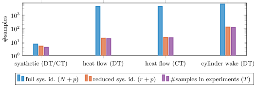
Figure 1: Number of data samples: In all experiments, the number of samples for control inference is lower than the number of samples required for learning a minimal model of the system. Furthermore, the number of samples is orders of magnitude lower than what would be required for learning traditional non-minimal models of the same dimension as the observed states. This is in agreement with Theorem 2 and the discussion in Section 3.2.

Figure 1 provides an overview about the number of data samples used in the following numerical experiments and how they compare to traditional two-step approaches that first identify either high- or low-dimensional models via system identification.

The experiments have been run on a machine equipped with an Intel(R) Core(TM) i7-8700 CPU at 3.20GHz and with 16 GB main memory. The algorithms are implemented in MATLAB 9.9.0.1467703 (R2020b) on CentOS Linux release 7.9.2009 (Core). For the solution of linear matrix inequalities, the disciplined convex programming toolbox CVX version 2.2, build 1148 (62bfcca) [31, 30] is used together with MOSEK version 9.1.9 [40] as inner optimizer. For the partial stabilization of identified systems, we use the implementations of the Bass’ algorithm for linear standard systems from the MORLAB toolbox version 5.0 [13, 12]. The code, data and results of the numerical experiments are available at [58].

5.1 Synthetic example

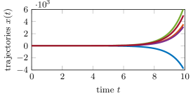
(a) DT: no controller.

(b) CT: no controller.

(c) DT: controller inference.

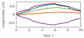
(d) CT: controller inference.

(e) DT: controller via system identification.

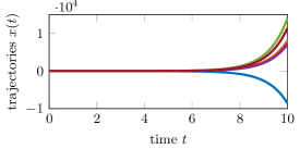
(f) CT: controller via system identification.

Figure 2: Synthetic example: The proposed inference approach leads to stabilizing controllers with data sets of only four samples in this example. In contrast, the classical two-step control procedure of first identifying a model and then constructing a controller leads to unstable dynamics in this example because of too few data samples in the data set, which is in agreement with Propositions 1 and 2.

Consider the system corresponding to the following state-space model

$$\begin{aligned} A_{0}&=\begin{bmatrix}-4&1&0&0&0\\ 1&-4&1&0&0\\ 0&1&1&1&0\\ 0&0&0&-4&1\\ 0&0&0&1&-4\end{bmatrix},&B_{0}&=\begin{bmatrix}1&0\\ 0&1\\ 0&0\\ 0&0\\ 0&0\end{bmatrix}\,,\end{aligned}$$

with state-space dimension $N=5$ and $p=2$ inputs. The dimension of the system is $n_{\min}=3$. The matrix $A_{0}$ is based on a spatial discretization of the two-dimensional Laplace operator, in which two disturbances are added such that $A_{0}$ is in upper block triangular form and has one controllable continuous-time unstable eigenvalue. The input matrix $B_{0}$ are the first two columns of the identity matrix. The initial condition is chosen to be homogeneous, $x_{0}=0$. To avoid trivially low-dimensional state vectors, the matrices $A_{0}$ and $B_{0}$ are transformed by an orthogonal matrix $Q$ with random entries. The continuous-time version of the considered state-space model is then given by

$$\begin{aligned} A_{\mathrm{ct}}&=Q^{\mkern-1.5mu\mathsf{T}}A_{0}Q,&B_{\mathrm{ct}}&=Q^{\mkern-1.5mu\mathsf{T}}B_{0}.\end{aligned}$$

The transformation does not change the size of the controllable system part, the eigenvalues of the system matrix or the zero initial condition. A discrete-time version of the example is obtained using the explicit Euler scheme with time step size $\tau=0.1$ on the continuous-time state-space model such that

$$\begin{aligned} A_{\mathrm{dt}}&=I_{n}+\tau A_{\mathrm{ct}},&B_{\mathrm{dt}}&=\tau B_{\mathrm{ct}}.\end{aligned}$$

The discrete-time state-space model has the same zero initial condition, the same dimension of the controllable system part and also one controllable unstable eigenvalue.

The trajectories of the discrete- and continuous-time state-space models are plotted in Figures 2(a) and 2(b), respectively. As expected for unstable systems, the trajectories do not converge to a finite stable behavior but tend to infinity.

We know from Corollaries 3 and 4 that $X_{-}$ from computed data $(U_{-},X_{-},X_{+})$ needs to have at least rank $3$ for the construction of a stabilizing feedback by informativity, i.e., due to the homogeneous initial condition, we need overall $T=4$ data samples. Note that for the identification of a minimal state-space model of the system, we need at least $n_{\min}+p=5$ data samples. The numerical rank of the collected data samples in $X_{-}$ and $X_{+}$ is in agreement with the minimal dimension of the system $n_{\min}=3$. We use Algorithm 1 to construct stabilizing feedbacks based on Theorem 2 directly from the obtained data using Propositions 2 and 1, i.e., without system identification. The trajectories corresponding to the stabilized systems are shown in Figures 2(c) and 2(d). Due to the closed-loop systems being stable, the trajectories converge to finite values for the given input signal. In contrast, because of too little data, the identified reduced state-space models do not contain unstable eigenvalues such that the feedbacks based on partial stabilization are zero. The closed-loop matrices with the identified feedbacks are unstable, as indicated by the trajectories in Figures 2(f) and 2(e).

5.2 Disturbed heat flow

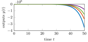
(a) DT: no controller.

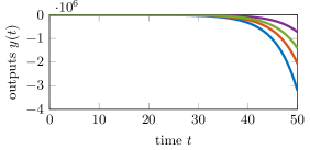
(b) CT: no controller.

(c) DT: controller inference.

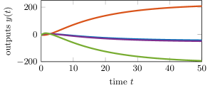
(d) CT: controller inference.

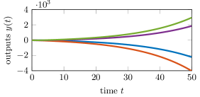
(e) DT: controller via system identification.

(f) CT: controller via system identification.

Figure 3: Heat flow: The controllers constructed via the inference approach stabilize the system. In contrast, applying the traditional two-step approach of first identifying a model and then controlling to the same data set only manages to decrease the growth of outputs but fails to stabilize the system in the discrete-time case. In case of the continuous-time system, the controller obtained from the identified model even accelerates the growth of the outputs and thus further destabilizes the system.

Consider now the system $\mathsf{HF2D5}$ described in [37]. It corresponds to a $2$-dimensional linear heat flow describing the heating process in a rectangular domain affected by disturbances; see [37, Sec. 3]. The spatial finite difference discretization yields a high-dimensional state-space model of dimension $N=4\,489$ with $p=2$ inputs and zero initial conditions. A discrete-time version of the model is obtained by using the implicit Euler discretization with time step size $\tau=0.1$. The discrete- and continuous-time versions of the model have a single unstable eigenvalue due to the modeled disturbance in the heating process. The measured outputs of the resulting time simulations using a unit step input signal are shown in Figures 3(a) and 3(b).

We employ Algorithm 1 in the approximate sense as discussed in Section 3.2. We computed $17$ samples in the discrete-time case to obtain an approximating subspace $\widetilde{\mathcal{V}}$ of dimension $r=17$. In the continuous-time case, we computed $20$ samples, which, due to the concatenation of the states and their time derivatives, resulted in a subspace of dimension $r=21$. In both cases, the subspaces are constructed to approximate the sampled states up to machine precision. We employ the re-projection approach from Algorithm 2 to get another data triplet $(U_{-},\widetilde{X}_{-},\widetilde{X}_{+})$ for the computations, since this leads to better numerical behavior of the linear matrix inequality solvers. In both cases, we computed $T=r+1$ data samples via re-projection. Note that at least $r+p=r+2$ samples are necessary for the unique identification of a reduced state-space model, i.e., the data set contains too few samples for system identification.

The controller inference leads in both cases to feedbacks that stabilize the systems. The corresponding simulations are shown in Figures 3(c) and 3(d). In contrast, the identified discrete-time reduced model has one unstable controllable eigenvalue like the original system, which is then stabilized via partial stabilization. Applying the lifted controller to the original system shifts the unstable eigenvalue closer to the unit circle; however, the shift is insufficient to stabilize the system. This can be seen in Figure 3(e), where the outputs are still diverging but slower than when no controller is applied. In the continuous-time case, the identified model has two complex conjugate unstable eigenvalues, which indicates that a different underlying system than the true one is approximated. The constructed feedback stabilizes the learned reduced model but, if applied to the true system, further destabilizes the system as shown in Figure 3(f).

5.3 Unstable laminar flow in a cylinder wake

(a) no controller.

(b) controller inference.

(c) controller via system identification.

Figure 4: Flow behind cylinder: In each sub figure, the top plot shows the magnitude of the high-dimensional state at final time and the bottom plot shows the averaged velocity in horizontal direction at four probes. Controller inference is able to stabilize the system, whereas traditional data-driven control via system identification fails when applied to the same data set.

We now consider the dynamics of a laminar flow inside a wake with a circular obstacle; see Figure 4 for the geometry. The flow is described by the Navier-Stokes equations. The steady state is known to behave unstable for medium and higher Reynolds numbers. The goal is to stabilize the system such that deviations from the steady state are steered back using controls in vertical and horizontal directions exactly behind the obstacle. We employ the setup from [5] at Reynolds number $90$ and consider a linearization of the Navier-Stokes equations around the desired steady state such that the linear system describes the deviation. This example is a linear system with $N=6\,618$ differential-algebraic equations (DAEs) and $p=6$ inputs describing the controls behind the obstacle in vertical and horizontal directions. The system has zero initial conditions. Due to the DAE form of the problem, we cannot directly obtain the time derivatives of the state. Therefore, we consider the example only in discrete-time form using the implicit Euler discretization with time step size $\tau=0.0025$. The resulting system has two unstable eigenvalues. For visualizations, four sensors are used in the back area of the wake that measure averaged velocities in horizontal and vertical directions. The trajectories obtained without control and the magnitudes of the state for the final time step are shown in Figure 4(a). As input, a disturbance is emulated in the time interval $[1,2]$ via a constant Gaussian step signal.

We take $180$ samples to compute an approximation $\widetilde{\mathcal{V}}$ of the reachability subspace of dimension $r=123$. We use Algorithm 2 to compute $r+2=125$ re-projected data samples for the design of stabilizing controllers. The inferred feedback design stabilizes the system and the trajectories, as shown by the state of the final time step in Figure 4(b). To improve the presentation of the stabilizing effect of the controller, it is only applied from time step $5$ onwards. The results show that the system stops oscillating and is steered back to the steady state.

In contrast, the state-space model we identified for the reduced re-projected data set does not have any unstable eigenvalues that could be stabilized. In fact, we know that the unique identification of a model would need at least four more data samples ($r+p=129$); cf. Proposition 1. As result, the constructed controller is zero and does not stabilize the original system as shown in Figure 4(c).

6 Conclusions and outlook

Learning from data becomes an ever more important component of scientific computing. Typically, the focus is on learning models of physical systems. Once a model is learned, classical scientific computing techniques can be applied to the learned models for solving upstream tasks such as control, design, and uncertainty quantification. However, learning models is only a means to an end in these cases. The ultimate goal is, e.g., finding an optimal design point and a controller, rather than learning models. This raises the question if it is necessary to learn models of complex physics that completely describe the systems of interest if the goal is solving potentially simpler upstream tasks. A similar question is asked in [41], which considers Monte Carlo estimation as the upstream task. It proposes to learn models specifically for the use as control variates for variance reduction. These models then can have large biases, which is not acceptable for making predictions about the system response but is sufficient for variance reduction. Another example is the work [21] that studies the learning of operators corresponding to linear Bayesian inverse problems in contrast to first learning a (forward) model and then inverting with classical scientific computing methods.

In this manuscript, we studied the task of stabilizing linear time-invariant systems. Building on previous work [56], our finding is that it is sufficient to have as many samples as the minimal dimension of the system, which is fewer than the minimal number of samples required for identifying a minimal model. Thus, it is unnecessary to learn models of the underlying systems when the task is stabilization under the assumptions we made, which results in lower data requirements. Given these findings, we believe understanding when learning models of systems is necessary is an important research direction, which is especially critical in large-scale science and engineering applications where the state dynamics are complex and data are scarce.

References

- [1] A. C. Antoulas. Approximation of Large-Scale Dynamical Systems, volume 6 of Adv. Des. Control. SIAM, Philadelphia, PA, 2005. doi:10.1137/1.9780898718713.
- [2] E. Armstrong. An extension of Bass’ algorithm for stabilizing linear continuous constant systems. IEEE Trans. Autom. Control, 20(1):153–154, 1975. doi:10.1109/TAC.1975.1100874.
- [3] E. Armstrong and G. Rublein. A stabilization algorithm for linear discrete constant systems. IEEE Trans. Autom. Control, 21(4):629–631, 1976. doi:10.1109/TAC.1976.1101295.
- [4] C. A. Beattie and S. Gugercin. Realization-independent -approximation. In 51st IEEE Conference on Decision and Control (CDC), pages 4953–4958, 2012. doi:10.1109/CDC.2012.6426344.
- [5] M. Behr, P. Benner, and J. Heiland. Example setups of Navier-Stokes equations with control and observation: Spatial discretization and representation via linear-quadratic matrix coefficients. e-print arXiv:1707.08711, arXiv, 2017. Mathematical Software (cs.MS). URL: https://arxiv.org/abs/1707.08711.
- [6] P. Benner, M. Castillo, E. S. Quintana-Ortí, and V. Hernández. Parallel partial stabilizing algorithms for large linear control systems. J. Supercomput., 15(2):193–206, 2000. doi:10.1023/A:1008108004247.
- [7] P. Benner, S. Gugercin, and K. Willcox. A survey of projection-based model reduction methods for parametric dynamical systems. SIAM Rev., 57(4):483–531, 2015. doi:10.1137/130932715.
- [8] P. Benner, J. Heiland, and S. W. R. Werner. Robust output-feedback stabilization for incompressible flows using low-dimensional -controllers. e-print 2103.01608, arXiv, 2021. Optimization and Control (math.OC). URL: https://arxiv.org/abs/2103.01608.
- [9] P. Benner, J.-R. Li, and T. Penzl. Numerical solution of large-scale Lyapunov equations, Riccati equations, and linear-quadratic optimal control problems. Numer. Lin. Alg. Appl., 15(9):755–777, 2008. doi:10.1002/nla.622.
- [10] P. Benner, W. Schilders, S. Grivet-Talocia, A. Quarteroni, G. Rozza, and L. M. Silveira. Model Order Reduction. Volume 1: System- and Data-Driven Methods and Algorithms. De Gruyter, Berlin, Boston, 2021. doi:10.1515/9783110498967.
- [11] P. Benner, W. Schilders, S. Grivet-Talocia, A. Quarteroni, G. Rozza, and L. M. Silveira. Model Order Reduction. Volume 2: Snapshot-Based Methods and Algorithms. De Gruyter, Berlin, Boston, 2021. doi:10.1515/9783110671490.
- [12] P. Benner and S. W. R. Werner. MORLAB – Model Order Reduction LABoratory (version 5.0), August 2019. see also: https://www.mpi-magdeburg.mpg.de/projects/morlab. doi:10.5281/zenodo.3332716.
- [13] P. Benner and S. W. R. Werner. MORLAB—The Model Order Reduction LABoratory. In P. Benner, T. Breiten, H. Faßbender, M. Hinze, T. Stykel, and R. Zimmermann, editors, Model Reduction of Complex Dynamical Systems, volume 171 of International Series of Numerical Mathematics, pages 393–415. Birkhäuser, Cham, 2021. doi:10.1007/978-3-030-72983-7_19.
- [14] J. Berberich, A. Koch, C. W. Scherer, and F. Allgöwer. Robust data-driven state-feedback design. In 2020 American Control Conference (ACC), pages 1532–1538, 2020. doi:10.23919/ACC45564.2020.9147320.
- [15] T. Breiten, R. Morandin, and P. Schulze. Error bounds for port-Hamiltonian model and controller reduction based on system balancing. Comput. Math. Appl., 116:100–115, 2021. doi:10.1016/j.camwa.2021.07.022.
- [16] S. L. Brunton, B. W. Brunton, J. L. Proctor, and J. N. Kutz. Koopman invariant subspaces and finite linear representations of nonlinear dynamical systems for control. PLoS ONE, 11(2):e0150171, 2016. doi:10.1371/journal.pone.0150171.
- [17] S. L. Brunton and J. N. Kutz. Data-Driven Science and Engineering:Machine Learning, Dynamical Systems, and Control. Cambridge University Press, Cambridge, 2019. doi:10.1017/9781108380690.
- [18] S. L. Brunton, J. L. Proctor, and J. N. Kutz. Discovering governing equations from data by sparse identification of nonlinear dynamical systems. Proc. Natl. Acad. Sci. U. S. A., 113(15):3932–3937, 2016. doi:10.1073/pnas.1517384113.
- [19] M. C. Campi, A. Lecchini, and S. M. Savaresi. Virtual reference feedback tuning: a direct method for the design of feedback controllers. Automatica J. IFAC, 38(8):1337–1346, 2002. doi:10.1016/S0005-1098(02)00032-8.
- [20] B. N. Datta. Numerical Methods for Linear Control Systems: Design and Analysis. Academic Press, San Diego, CA, 2004. doi:10.1016/B978-0-12-203590-6.X5000-9.
- [21] M. V. De Hoop, N. B. Kovachki, N. H. Nelsen, and A. M. Stuart. Convergence rates for learning linear operators from noisy data. e-print 2108.12515, arXiv, 2021. Statistics Theory (math.ST). URL: https://arxiv.org/abs/2108.12515.
- [22] C. De Persis and P. Tesi. Formulas for data-driven control: Stabilization, optimality, and robustness. IEEE Trans. Autom. Control, 65(3):909–924, 2020. doi:10.1109/TAC.2019.2959924.
- [23] S. Dean, H. Mania, N. Matni, B. Recht, and Tu S. On the sample complexity of the linear quadratic regulator. Found. Comput. Math., 20(4):633–679, 2020. doi:10.1007/s10208-019-09426-y.
- [24] V. Dragan and A. Halanay. Stabilization of Linear Systems. Systems & Control: Foundations & Applications. Birkhäuser, Boston, MA, 1999. doi:10.1007/978-1-4612-1570-7.
- [25] Z. Drmač, I. Mezić, and R. Mohr. Data driven modal decompositions: Analysis and enhancements. SIAM J. Sci. Comput., 40(4):A2253–A2285, 2018. doi:10.1137/17M1144155.
- [26] M. Fliess and C. Join. Model-free control. Int. J. Control, 86(12):2228–2252, 2013. doi:10.1080/00207179.2013.810345.
- [27] M. Gevers, A. S. Bazanella, X. Bombois, and L. Miskovic. Identification and the information matrix: How to get just sufficiently rich? IEEE Trans. Autom. Control, 54(12):2828–2840, 2009. doi:10.1109/TAC.2009.2034199.
- [28] G. H. Golub and C. F. Van Loan. Matrix Computations. Johns Hopkins Studies in the Mathematical Sciences. Johns Hopkins University Press, Baltimore, fourth edition, 2013.
- [29] I. V. Gosea, S. Gugercin, and C. Beattie. Data-driven balancing of linear dynamical systems. e-print 2104.01006, arXiv, 2021. Numerical Analysis (math.NA). URL: https://arxiv.org/abs/2104.01006.
- [30] M. Grant and S. Boyd. CVX: Matlab software for disciplined convex programming, version 2.2. http://cvxr.com/cvx, January 2020.
- [31] M. C. Grant and S. P. Boyd. Graph implementations for nonsmooth convex programs. In V. D. Blondel, S. P. Boyd, and H. Kimura, editors, Recent Advances in Learning and Control, volume 371 of Lect. Notes Control Inf. Sci., pages 95–110. Springer, London, 2008. doi:10.1007/978-1-84800-155-8\_7.
- [32] E. A. Jonckheere and L. M. Silverman. A new set of invariants for linear systems–application to reduced order compensator design. IEEE Trans. Autom. Control, 28(10):953–964, 1983. doi:10.1109/TAC.1983.1103159.
- [33] E. Kaiser, J. N. Kutz, and S. L. Brunton. Sparse identification of nonlinear dynamics for model predictive control in the low-data limit. Proc. R. Soc. A: Math. Phys. Eng. Sci., 474(2219):20180335, 2018. doi:10.1098/rspa.2018.0335.
- [34] E. Kaiser, J. N. Kutz, and S. L. Brunton. Data-driven discovery of Koopman eigenfunctions for control. Mach. Learn.: Sci. Technol., 2(3):035023, 2021. doi:10.1088/2632-2153/abf0f5.
- [35] B. Kramer, B. Peherstorfer, and K. Willcox. Feedback control for systems with uncertain parameters using online-adaptive reduced models. SIAM J. Appl. Dyn. Syst., 16(3):1563–1586, 2017. doi:10.1137/16M1088958.
- [36] P. Lancaster and L. Rodman. Algebraic Riccati Equations. Oxford Science Publications. The Clarendon Press, Oxford University Press, New York, 1995.
- [37] F. Leibfritz. : COnstrained Matrix-optimization Problem library – a collection of test examples for nonlinear semidefinite programs, control system design and related problems. Tech.-report, University of Trier, 2004. URL: http://www.friedemann-leibfritz.de/COMPlib_Data/COMPlib_Main_Paper.pdf.
- [38] O. Lequin, M. Gevers, M. Mossberg, E. Bosmans, and L. Triest. Iterative feedback tuning of PID parameters: comparison with classical tuning rules. Control Eng. Pract., 11(9):1023–1033, 2003. doi:10.1016/S0967-0661(02)00303-9.
- [39] A. J. Mayo and A. C. Antoulas. A framework for the solution of the generalized realization problem. Linear Algebra Appl., 425(2–3):634–662, 2007. Special issue in honor of P. A. Fuhrmann, Edited by A. C. Antoulas, U. Helmke, J. Rosenthal, V. Vinnikov, and E. Zerz. doi:10.1016/j.laa.2007.03.008.
- [40] MOSEK ApS. The MOSEK optimization toolbox for MATLAB manual. Version 9.1.9, November 2019. URL: https://docs.mosek.com/9.1/toolbox/index.html.
- [41] B. Peherstorfer. Multifidelity Monte Carlo estimation with adaptive low-fidelity models. SIAM/ASA J. Uncertainty Quantification, 7(2):579–603, 2019. doi:10.1137/17M1159208.
- [42] B. Peherstorfer. Sampling low-dimensional Markovian dynamics for preasymptotically recovering reduced models from data with operator inference. SIAM J. Sci. Comput., 42(5):A3489–A3515, 2020. doi:10.1137/19M1292448.
- [43] B. Peherstorfer, S. Gugercin, and K. Willcox. Data-driven reduced model construction with time-domain Loewner models. SIAM J. Sci. Comput., 39(5):A2152–A2178, 2017. doi:10.1137/16M1094750.
- [44] B. Peherstorfer and K. Willcox. Data-driven operator inference for nonintrusive projection-based model reduction. Comput. Methods Appl. Mech. Eng., 306:196–215, 2016. doi:10.1016/j.cma.2016.03.025.
- [45] A. Quarteroni and G. Rozza. Reduced Order Methods for Modeling and Computational Reduction, volume 9 of MS&A – Modeling, Simulation and Applications. Springer, Cham, 2014. doi:10.1007/978-3-319-02090-7.
- [46] H. H. Rosenbrock. State-space and Multivariable Theory, volume 3 of Studies in dynamical systems. Wiley, New York, 1970.
- [47] M. G. Safonov and T.-C. Tsao. The unfalsified control concept: A direct path from experiment to controller. In B. .A Francis and A. R. Tannenbaum, editors, Feedback Control, Nonlinear Systems, and Complexity, volume 202 of Lect. Notes Control Inf. Sci., pages 196–214. Springer, Berlin, Heidelberg, 1995. doi:10.1007/BFb0027678.
- [48] H. Schaeffer, R. Caflisch, C. D. Hauck, and S. Osher. Sparse dynamics for partial differential equations. Proc. Natl. Acad. Sci. U. S. A., 110(17):6634–6639, 2013. doi:10.1073/pnas.1302752110.
- [49] H. Schaeffer, G. Tran, and R. Ward. Extracting sparse high-dimensional dynamics from limited data. SIAM J. Appl. Math., 78(6):3279–3295, 2018. doi:10.1137/18M116798X.
- [50] P. J. Schmid. Dynamic mode decomposition of numerical and experimental data. J. Fluid Mech., 656:5–28, 2010. doi:10.1017/S0022112010001217.
- [51] P. Schulze and B. Unger. Data-driven interpolation of dynamical systems with delay. Syst. Control Lett., 97:125–131, 2016. doi:10.1016/j.sysconle.2016.09.007.
- [52] P. Schulze, B. Unger, C. Beattie, and S. Gugercin. Data-driven structured realization. Linear Algebra Appl., 537:250–286, 2018. doi:10.1016/j.laa.2017.09.030.
- [53] J. H. Tu, C. W. Rowley, D. M. Luchtenburg, S. L. Brunton, and J. N. Kutz. On dynamic mode decomposition: Theory and applications. J. Comput. Dyn., 1(2):391–421, 2014. doi:10.3934/jcd.2014.1.391.
- [54] S. Tu, R. Boczar, A. Packard, and B. Recht. Non-asymptotic analysis of robust control from coarse-grained identification. e-print 1707.04791, arXiv, 2017. Optimization and Control (math.OC). URL: https://arxiv.org/abs/1707.04791.
- [55] P. Van Overschee and B. De Moor. Subspace Identification for Linear Systems: Theory, Implementation, Applications. Springer, Boston, MA, 1996. doi:10.1007/978-1-4613-0465-4.
- [56] H. J. Van Waarde, J. Eising, H. L. Trentelman, and M. K. Camlibel. Data informativity: A new perspective on data-driven analysis and control. IEEE Trans. Autom. Control, 65(11):4753–4768, 2020. doi:10.1109/TAC.2020.2966717.
- [57] M. Voigt. On Linear-Quadratic Optimal Control and Robustness of Differential-Algebraic Systems. Dissertation, Otto-von-Guericke-Universität, Magdeburg, Germany, 2015.
- [58] S. W. R. Werner. Code, data and results for numerical experiments in “On the sample complexity of stabilizing linear dynamical systems from data” (version 1.0), February 2022. doi:10.5281/zenodo.5902997.
- [59] J. C. Willems, P. Rapisarda, I. Markovsky, and B. L. M. De Moor. A note on persistency of excitation. Syst. Control Lett., 54(4):325–329, 2005. doi:10.1016/j.sysconle.2004.09.003.
- [60] J. Ziegler and N. Nichols. Optimum settings for automatic controllers. Trans. ASME, 64:759–768, 1942.