Low-luminosity type IIP supernovae: SN 2005cs and SN 2020cxd as very low-energy iron core-collapse explosions

Abstract

SN 2020cxd is a representative of the family of low-energy, underluminous Type IIP supernovae (SNe), whose observations and analysis were recently reported by Yang et al. (2021). Here we re-evaluate the observational data for the diagnostic SN properties by employing the hydrodynamic explosion model of a 9 M_⊙ red supergiant progenitor with an iron core and a pre-collapse mass of 8.75 M_⊙. The explosion of the star was obtained by the neutrino-driven mechanism in a fully self-consistent simulation in three dimensions (3D). Multi-band light curves and photospheric velocities for the plateau phase are computed with the one-dimensional radiation-hydrodynamics code STELLA, applied to the spherically averaged 3D explosion model as well as sphericized radial profiles in different directions of the 3D model. We find that the overall evolution of the bolometric light curve, duration of the plateau phase, and basic properties of the multi-band emission can be well reproduced by our SN model with its explosion energy of only $0.7\times 10^{50}$ erg and an ejecta mass of 7.4 M_⊙. These values are considerably lower than the previously reported numbers, but they are compatible with those needed to explain the fundamental observational properties of the prototype low-luminosity SN 2005cs. Because of the good compatibility of our photospheric velocities with line velocities determined for SN 2005cs, we conclude that the line velocities of SN 2020cxd are probably overestimated by up to a factor of about 3. The evolution of the line velocities of SN 2005cs compared to photospheric velocities in different explosion directions might point to intrinsic asymmetries in the SN ejecta.

1 Introduction

The recently discovered supernova (SN) 2020cxd is a low-luminosity hydrogen-rich type II SN (LL type IIP SN, Yang et al., 2021; Valerin et al., 2022). Due to its low plateau luminosity of about $10^{\,41}$ erg s${}^{\,-1}$ and relatively low photospheric velocity at the end of the plateau, it is considered to be a member of the family of LL type IIP SNe (e.g., Pastorello et al., 2009; Spiro et al., 2014; Reguitti et al., 2021). Analysing the bolometric light curve, Yang et al. (2021) inferred the explosion of a red supergiant (187 $\mathrm{R}_{\odot}$) with a pre-collapse mass of about 11 $\mathrm{M}_{\odot}$ (and a zero-age main sequence (ZAMS) mass of about 12 $\mathrm{M}_{\odot}$) and an energy of 0.58 foe (1 foe $=10^{\,51}$ erg). SN 2020cxd exhibits a large drop between the plateau and the radioactive tail, as well as a very low tail luminosity. The total mass of the ejected radioactive nickel ⁵⁶Ni is 0.003 $\mathrm{M}_{\odot}$. More recently, Valerin et al. (2022) found that the best-fit SN parameters are an ejecta mass of 7.5 $\mathrm{M}_{\odot}$, explosion energy of 0.097 foe, and a progenitor radius of 575 $\mathrm{R}_{\odot}$. These values are in fairly satisfactory agreement with the results we will report in our paper.

We note in passing that besides their relevance for stellar and SN astrophysics, LL type IIP SNe are also of great interest for setting constraints to physics beyond the Standard Model (BSM) of particle physics (Caputo et al., 2022a). BSM particle production might play a role at the high densities and temperatures in new-born neutron stars. This could extract energy from the compact remnant during the neutrino-cooling phase and would thus change the observable neutrino signal (e.g., Chang et al., 2018; Carenza et al., 2019; Caputo et al., 2022b), and it could also have an impact on the SN energetics, dynamics, and electromagnetic emission in various ways (e.g., Rembiasz et al., 2018; Mori et al., 2022; Caputo et al., 2022a).

According to the current understanding, based on recent self-consistent 3-dimensional (3D) simulations of the underlying mechanism that causes the explosion of massive stars, SNe with a plateau in their light curves result from the neutrino-driven mechanism (e.g., Takiwaki et al., 2014; Lentz et al., 2015; Melson et al., 2015a; Melson et al., 2015b; Müller et al., 2017a, 2018; Ott et al., 2018; Summa et al., 2018; Burrows et al., 2019; Glas et al., 2019; Stockinger et al., 2020; Bollig et al., 2021). The amount of radioactive nickel ⁵⁶Ni produced in this kind of explosion is proportional to the neutrino luminosity and amount of ejecta material heated by neutrinos. The higher the neutron-star mass (correlated with the progenitor’s compactness as defined by O’Connor & Ott 2011) the higher the neutrino luminosity, the bigger the amount of neutrino-heated ejecta, the more energetic the shock wave, and the larger the mass of radioactive nickel (Nakamura et al., 2015; Ertl et al., 2016; Müller et al., 2016; Sukhbold et al., 2016; Janka, 2017; Ertl et al., 2020). These dependencies associated with neutrino-driven explosions are in line with correlations between SN energies, ⁵⁶Ni masses and plateau luminosities deduced from observations (Pejcha & Prieto, 2015a; Müller et al., 2017b; Pejcha, 2020). Recent studies show that the reference amount of ejected radioactive nickel ⁵⁶Ni is about 0.03 $\mathrm{M}_{\odot}$ for a diagnostic explosion energy around 0.6 foe (Müller et al., 2016, 2017a; Ertl et al., 2020). Therefore, the parameters of SN 2020cxd diagnosed by Yang et al. (2021) are in conflict with our current theoretical and observational picture of the underlying physics of core-collapse SN explosions. Motivated by this fact we present here a revision of the analysis made by Yang et al. (2021) with the effort to find a more reliable interpretation for the progenitor of SN 2020cxd and its explosion. We also choose SN 2005cs as a representative member of the family of LL type IIP SNe, because SN 2005cs has a better data coverage, and analyse SN 2020cxd together with SN 2005cs in the context of our theoretical model.

In Section 2 we describe our considered SN model and the radiation-hydrodynamics treatment with the STELLA code. In Section 3 we present bolometric and multi-band light curves as well as photospheric velocities and colours of our model calculations in comparison to observational data for SN 2020cxd and SN 2005cs, including an assessment of the line velocities reported for SN 2020cxd in the literature. In Section 4 we summarize our results and draw conclusions. Appendices A, B, and C present angle-averaged and direction dependent profiles for our considered 3D SN model as well as corresponding multi-band light curves and the colour evolution of the SN calculations.

2 Input model and Method

Table 1: Parameters of the LL type IIP SNe 2020cxd, 2005cs, and the angle-averaged parameters of model s9.0. $t_{\mathrm{p}}$ is the duration of plateau phase which ends at the middle of the transition to the radioactive tail. Velocity gives the H$\alpha$ line velocity for SN 2020cxd and the Sc ii line velocity for SN 2005cs around the middle of the plateau, radius is the progenitor radius at the pre-collapse stage, $M_{\mathrm{ej}}$ the ejecta mass, $M_{\mathrm{prog}}$ the progenitor mass, $M_{{}^{56}\mathrm{Ni}}$ the ejected mass of ⁵⁶Ni, and $E_{\mathrm{expl}}$ the explosion energy (for model s9.0 to be identified with $E_{\mathrm{kin}}$ in Table 2).

SN	$M_{\mathrm{bol}}$	$t_{\mathrm{p}}$	Velocity	Radius	$M_{\mathrm{ej}}$	$M_{\mathrm{prog}}$	$M_{{}^{56}\mathrm{Ni}}$	$E_{\mathrm{expl}}$	Reference
	[mags]	[days]	[1000 km s${}^{\,-1}$]	[$\mathrm{R}_{\odot}$]	[$\mathrm{M}_{\odot}$]	[$\mathrm{M}_{\odot}$]	[$\mathrm{M}_{\odot}$]	foe
2020cxd	$-$14.0	130	4	187	9.5		0.003	0.58	Yang et al. (2021)
				575	7.5		0.0018	0.097	Valerin et al. (2022)
2005cs	$-$14.58	130	1.5	100	11.1		0.0028	0.3	Pastorello et al. (2009)
				357	9.5		0.006	0.16	Pumo et al. (2017)
				600	15.9	18.2	0.0082	0.41	Utrobin & Chugai (2008)
s9.0				408	7.4	8.75	0.003	0.068	present study

In Table 1, we report the published properties of SN 2005cs as a representative member of the family of LL type IIP SNe and of the low-luminosity SN 2020cxd, and confront them with the properties of our theoretical model. We consider a star near the low-mass end of SN progenitors with an initial mass of 9 $\mathrm{M}_{\odot}$ (Sukhbold et al., 2016) as the most suitable model. A low-energy neutrino-driven explosion of such a low-mass progenitor can explain LL type IIP SNe, as was already discussed by a number of observational and theoretical studies (Mattila et al., 2008; Van Dyk et al., 2012; Jerkstrand et al., 2018). We note that the study by Utrobin & Chugai (2008) explains SN 2005cs with an explosion of a higher-mass progenitor of 18.2 $\mathrm{M}_{\odot}$, however, their study was based on a non-evolutionary progenitor configuration. A connection with the explosion of such a high-mass progenitor, however, is disfavoured by recent self-consistent 3D models of neutrino-driven explosions of 18 – 19 $\mathrm{M}_{\odot}$ stars (Müller et al., 2017a; Bollig et al., 2021).

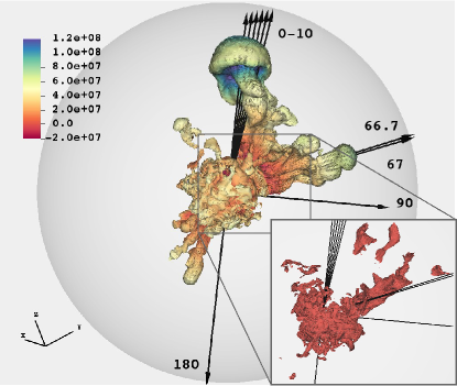
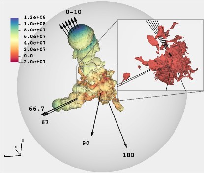
Figure 1: Three-dimensional explosion geometry of the s9.0 model (Stockinger et al., 2020) used as input for the present study. The two panels show different views of the isosurface of a constant ⁵⁶Ni mass fraction of 0.01 at 1.974 days after core collapse ($\sim$0.2 days before the fastest part of the deformed SN shock reaches the stellar surface), with the radial velocity (in units of cm s${}^{\,-1}$) colour-coded. The zoom insets show the isosurface of a constant ⁵⁶Ni mass fraction of 0.1 with the same colour-coding. The semi-transparent grey sphere marks the stellar surface (at a radius of $2.86\times 10^{\,13}$ cm). Black arrows denote the selected angular directions as listed in Table 2; for reasons of clarity we do not show the “$-$” directions (i.e., $-2^{\circ}$ to $-10^{\circ}$), which are distinguished from the “$+$” directions ($+2^{\circ}$ to $+10^{\circ}$) by an azimuthal angular shift of 180^∘ around the major ⁵⁶Ni plume axis (i.e., the 0^∘ direction).

Our progenitor model of a star with an initial mass of 9 $\mathrm{M}_{\odot}$ (model s9.0 of Sukhbold et al. 2016) was computed with the stellar evolution code KEPLER (Weaver et al., 1978) until the onset of iron-core collapse (Woosley & Heger, 2015). A one-dimensional (1D) SN simulation of this model, which was exploded parametrically via neutrino heating by Ertl et al. (2016) and Sukhbold et al. (2016), led to an explosion energy of 0.11 foe. This explosion model was later used for nebular spectral modeling by Jerkstrand et al. (2018). The corresponding self-consistent 3D simulation of a neutrino-driven explosion of this 9 M_⊙ progenitor model with the PROMETHEUS-VERTEX code was first discussed in Melson et al. (2020) and was later used for long-time 3D simulations with PROMETHEUS-HOTB by Stockinger et al. (2020). Independently, the s9.0 model was successfully exploded in 3D by Glas et al. (2019) and by Burrows et al. (2019).

For our present work we use the s9.0 model of Stockinger et al. (2020), which has already been used as input for the study by Kozyreva et al. (2021). We note that an improved post-processing analysis is applied in the present work and the profiles are extracted from the 3D simulation at an earlier epoch, namely at 1.974 days (instead of 2.823 days) after core collapse. At this moment the fastest parts of the shock are within 0.2 days before their breakout from the stellar surface. The shock front is strongly deformed, and the slowest parts of the shock reach the stellar surface only approximately 1 day later, i.e. about 3.1 days after the onset of the explosion. In Appendix A, we present comparative plots showing the structure of the angle-averaged profiles used in Kozyreva et al. (2021) compared to the profiles used as input in the present work. The geometry of the shock front is far from spherical symmetry and the distribution of the ejected ⁵⁶Ni displays a main plume and a few smaller plumes of high-entropy material. We illustrate the asphericity of the model in Figure 1. In total we extract 16 radial profiles which represent the structure of the ejecta in different angular directions of the 3D model. The profiles are listed in Table 2 and are named according to the angle relative to the central-axis direction of the fastest plume of the ejected ⁵⁶Ni (see Figure 1). The velocity and density profiles along with the distribution of the ⁵⁶Ni mass fraction in each of the different radial directions are shown in Appendix B. We note that the value of the explosion energy of 0.048 foe as given in Table 4 of Stockinger et al. (2020) is taken at the end of the PROMETHEUS-VERTEX simulation at 3.14 s, whereas we give the value at 1.974 days from the long-time continuation run with the PROMETHEUS-HOTB code.

In the current study, the 3D explosion model is mapped into the 1D radiation-hydrodynamics code STELLA (Blinnikov et al., 2006). STELLA is capable of processing hydrodynamics as well as the radiation field evolution, i.e. computing light curves, spectral energy distribution and resulting broad-band magnitudes and colours. We use the standard parameter settings, well-explained in many papers involving STELLA simulations (see e.g., Kozyreva et al., 2019; Moriya et al., 2020). The thermalisation parameter, which accounts for the treatment of the line opacity and expresses the ratio between absorption and scattering opacities, is set to 0.9 as recommended by the recent study by Kozyreva et al. (2020). The profiles along different radial directions are sphericized during the mapping into STELLA. The corresponding 4$\pi$-equivalent values of different quantities are listed in Table 2. The total amount of ⁵⁶Ni is scaled to 0.003 $\mathrm{M}_{\odot}$ to match the mass of ⁵⁶Ni estimated for SN 2020cxd (Yang et al., 2021). A value of the ⁵⁶Ni (plus ⁵⁶Co and ⁵⁶Fe) yield of 0.00635 $\mathrm{M}_{\odot}$ was reported by Stockinger et al. (2020) for the 3D explosion model of s9.0 and recently determined to be 0.0057 $\mathrm{M}_{\odot}$ by a more accurate re-evaluation of the simulation outputs (see data in https://wwwmpa.mpa-garching.mpg.de/ccsnarchive/data/Stockinger2020/). Note that the angle-averaged profile in Kozyreva et al. (2021) had 0.005 $\mathrm{M}_{\odot}$ of ⁵⁶Ni. We mention two reasons why a rescaling of the ⁵⁶Ni mass is well motivated:

1. The nucleosynthesis calculations yielding the values reported by Stockinger et al. (2020) and re-evaluated in the present study were only approximate, because they were based on the use of a small nuclear $\alpha$-chain network.

2. The exact amount of ⁵⁶Ni produced in 3D explosion models is extremely sensitive to the electron fraction ($Y_{e}$) in the neutrino-heated ejecta, which is determined by the interaction of the innermost ejecta with the intense neutrino radiation from the proto-neutron star. Therefore, the $Y_{e}$ distribution in these ejecta depends sensitively on the details of the neutrino physics and neutrino transport, including the still incompletely understood effects of neutrino-flavor oscillations in and near the proto-neutron star.

The uncertainties in the exact ejected mass of ⁵⁶Ni corresponding to these points can well amount to a factor of 2.

Table 2: Isotropic-equivalent parameter values for the profiles corresponding to different radial directions and for the angle-averaged profile (labeled “AVG”) taken from the 3D model s9.0 (Stockinger et al., 2020). The name of the direction represents the angle from the axis of the main high-entropy plume. For the cases of $2^{\circ}$–$10^{\circ}$ we show two (“$+$” and “$-$”) directions, which are distinguished by an azimuthal angular shift of 180^∘ around the axis of the major ⁵⁶Ni plume (i.e., the $0^{\circ}$ direction). The total mass of radioactive ⁵⁶Ni is a sum of ⁵⁶Ni and its daughter products ⁵⁶Co and ⁵⁶Fe. Note that we list the ⁵⁶Ni mass ($M_{\mathrm{{}^{56}Ni}}$) with the value that is present in each of the profiles before scaling to 0.003 $\mathrm{M}_{\odot}$ needed to match the mass of ⁵⁶Ni in SN 2020cxd and SN 2005cs. $M_{\mathrm{tot}}$ is the isotropic-equivalent total mass including the central compact object, while $M_{\mathrm{ej}}$ is the isotropic equivalent of the ejected mass. $E_{\mathrm{expl}}$ is the $4\pi$-equivalent explosion energy at 1.974 days. $E_{\mathrm{kin}}$ is the analogously determined terminal kinetic energy at the end of the radiative transfer simulations (at day 170), before and after scaling the ⁵⁶Ni mass to 0.003 M_⊙. The energy difference is a consequence of the different release of energy in radioactive ⁵⁶Ni and ⁵⁶Co decay which contributes to the energy balance after the energies of $\gamma$-rays and positrons are thermalised.

direction	$M_{\mathrm{{}^{56}Ni}}$	$M_{\mathrm{tot}}$	$M_{\mathrm{ej}}$	$E_{\mathrm{expl}}$	$E/M$	$E_{\mathrm{kin}}$
	[M⊙]	[M⊙]	[M⊙]	[0.1 foe]	[foe/M⊙]	[0.1 foe]
0∘	0.0974	5.75	4.40	1.2812	0.0303	1.3337/1.2641
$+$2∘	0.0886	5.96	4.61	1.3069	0.0293	1.3502/1.2915
$-$2∘	0.0951	5.48	4.13	1.1885	0.0299	1.2362/1.1701
$+$4∘	0.1229	6.14	4.79	1.2964	0.0286	1.3684/1.2801
$-$4∘	0.1150	5.70	4.35	1.1553	0.0278	1.2110/1.1289
$+$6∘	0.1278	6.23	4.88	1.1894	0.0259	1.2626/1.1641
$-$6∘	0.0947	5.79	4.44	1.0850	0.0253	1.1233/1.0543
$+$8∘	0.0947	6.38	5.03	1.0524	0.0217	1.0931/1.0177
$-$8∘	0.0540	5.85	4.50	0.9425	0.0210	0.9459/0.9070
$+$10∘	0.0814	6.50	5.15	0.8836	0.0177	0.9122/0.8445
$-$10∘	0.0460	6.12	4.77	0.7960	0.0166	0.7930/0.7583
66.7∘	0.0659	8.68	7.32	0.8026	0.0117	0.8594/0.7951
67∘	0.0582	8.66	7.31	0.8030	0.0117	0.8523/0.7964
90∘	0.0010	8.75	7.40	0.7596	0.0102	0.7524/0.7544
180∘	0.0026	8.80	7.45	0.6943	0.0092	0.6884/0.6887
AVG	0.0057	8.75	7.40	0.7334	0.0095	0.6790/0.6765

Recently, radiative transfer simulations with the spherically averaged 3D explosion model of s9.0 were done in a separate paper and compared to the LL type IIP SNe 2005cs and 1999br (Kozyreva et al., 2021). The model matches the broad-band magnitudes and bolometric light curves of these observed SNe. The comparison demonstrates the applicability of the given model for LL type IIP SNe. Hence, it has already been shown that our explosion model of the 9 $\mathrm{M}_{\odot}$ progenitor is capable of explaining a number of members of the family of LL type IIP SNe.

3 Results

3.1 Bolometric properties

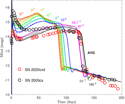
Figure 2: Bolometric light curves (in absolute magnitudes) for different radial directions of model s9.0, and LL type IIP SNe 2005cs and 2020cxd. The label “AVG” represents the light curve for the angle-averaged profile. The solid and dashed curves indicate the “$+$” and “$-$” directions for the cases of 2^∘–10^∘, as introduced in Table 2.

In Figure 2 bolometric light curves for different radial directions of our 3D explosion simulation and the angle-averaged case of model s9.0 are displayed. We superpose bolometric light curves of two LL type IIP SNe, SN 2020cxd and SN 2005cs. Our 66.7^∘, 67^∘, 90^∘, 180^∘, and angle-averaged cases are capable of matching the bolometric light curve of SN 2020cxd to a very large extent without any artificial tuning besides a proper scaling of the ⁵⁶Ni mass to match the observationally determined value (see Section 2). And they are also able to reproduce the global behaviour of the bolometric light curve of SN 2005cs.

Because the explosion energy is a crucial factor governing the plateau luminosity (Arnett, 1980; Popov, 1993; Kasen & Woosley, 2009; Sukhbold et al., 2016; Goldberg et al., 2019; Kozyreva et al., 2019), a luminosity of a Type IIP SN as low as $L\simeq 10^{\,41}$ erg s${}^{\,-1}$ or –14 mags (average for the LL type IIP family) can be reproduced by very low explosion energies, around or below 0.1 foe for stars near the low-mass end of core-collapse SN progenitors (Pumo et al., 2017). The V-band magnitude ($V$) and the bolometric luminosity ($L$) at the middle of the plateau are:

$$\begin{array}[]{l}V\sim 1.25\log M-2.08\log E-1.67\log R\,,\\ \log L\sim-0.4\log M+0.74\log E+0.76\log R\,,\end{array}$$ (1)

where $M$ is the ejecta mass, $E$ the explosion energy, and $R$ the progenitor radius prior to the explosion. The scaling relations are taken from Popov (1993) and Goldberg et al. (2019), respectively. Note that we neglect the additive terms given in these references, because we are only interested in the dependencies. If the energy varies between 0.03 foe and 1.5 foe (Ertl et al., 2016; Stockinger et al., 2020), this corresponds to $-$1.5 and 0.2 in logarithmic scale, which results in a luminosity scatter up to 1 dex. The low explosion energy required for low-luminosity events can be released in low-mass progenitors of 9–10 $\mathrm{M}_{\odot}$, as the energy exhibits a (rough) tendency to increase with the initial progenitor mass (Nakamura et al., 2015; Ertl et al., 2016; Müller et al., 2016; Pejcha, 2020). The second strongest factor is the progenitor radius, and the weakest effect is connected to the ejecta mass. The radius ranges between 100 $\mathrm{R}_{\odot}$ and a few 1000 $\mathrm{R}_{\odot}$ for the observed red-supergiants (Levesque et al., 2005; Levesque et al., 2006). This leads to a scatter in luminosity of 0.76 dex. The ejecta mass tends to be around 10 $\mathrm{M}_{\odot}$ and has a relatively less important effect. To reach very low luminosities, the radius of the progenitors should not be very large, yet it should still allow for sufficient recombination to power the light curve (Grasberg & Nadezhin, 1976) and to provide an extended plateau phase, since shrinking the progenitor radius shortens the duration of the plateau:

$$\begin{array}[]{l}\log t_{\mathrm{p}}\sim 0.5\log M-0.167\log E+0.167\log R\,,\\ \log t_{\mathrm{p}}\sim 0.41\log M-0.28\log E-0.02\log R\,+0.13\log M_{\mathrm{Ni}}\,,\end{array}$$ (2)

where $t_{\mathrm{p}}$ is the plateau duration, $M$, $E$, and $R$ have the same meaning as in Equation 1, and $M_{\mathrm{Ni}}$ is the total mass of radioactive ⁵⁶Ni. The relations are taken from Popov (1993) and Goldberg et al. (2019), respectively. Note that the updated scaling relation for the plateau duration from Goldberg et al. (2019) does not show a strong dependence on the progenitor radius. Even though the highest exponent is in the mass term, the mass does not strongly affect the variations of the duration since the ejecta mass is always close to 10 $\mathrm{M}_{\odot}$. The influence of radioactive nickel in the ejecta on the plateau luminosity is moderate, whereas the plateau duration is strongly affected by the presence of nickel and its distribution (Kozyreva et al., 2019). However, for low-mass explosions, which we consider as the most probable explanation for the LL type IIP SNe, the ⁵⁶Ni yield is a few thousandths of a solar mass and does not extend the length of the plateau and its luminosity value to any significant extent (see Kozyreva et al., 2021).

The light curves for the directions aligned with the fastest parts of the s9.0 ejecta, i.e. close to the directions of $0^{\circ}-10^{\circ}$, do not match the given observed LL type IIP SNe. Nevertheless, we presume that flux from these angles may contribute to other directions. To clarify the question on the contributions of other radial directions to the particular viewing direction, realistic 3D radiative-transfer simulations are required, which may be carried out in the future.

Interestingly, the bolometric light curve during the plateau increases for SN 2020cxd until shortly before the steep decline to the nickel tail, which is amazingly well reproduced by our explosion model for the angle-averaged profiles and the directions at 66.7^∘, 67^∘, 90^∘, and 180^∘. In contrast, SN 2005cs shows nearly a flat plateau and after the middle of the plateau a shallow decline sets in well before the steep drop to the radioactive tail. Such a difference in the shape of the plateau was discussed in Kozyreva et al. (2019). It could, in principle, be connected to different degrees of mixing of radioactive ⁵⁶Ni. In the context of the considered LL type IIP SNe, however, this explanation is disfavored by the small mass of only 0.003 M_⊙ of ejected ⁵⁶Ni (Kozyreva et al., 2021).

The different light-curve shapes of SN 2005cs and SN 2020cxd might instead be a hint of a considerable degree of explosion asymmetry in the former case, even already during the shock-breakout phase and during the early expansion of the hydrogen envelope. Such a possibility for SNe of low-mass progenitors is suggested by the extreme deformation of the ejecta associated with the largest nickel plume in our 3D explosion model s9.0. This nickel-rich plume extends through the entire hydrogen envelope and pushes the expansion of the SN shock wave. Therefore, when the head of the plume reaches the stellar surface, the shock breaks out roughly 1 day earlier than in the other directions (see Stockinger et al. 2020 and our discussion in Section 2 connected to Figure 1). The light curves computed for sphericized ejecta conditions in different directions of our 3D explosion model (as displayed in Figure 2) suggest the possible influence of such explosion asymmetries. In the directions from 0^∘ to 10^∘ relative to the axis of the biggest nickel-rich plume, the higher explosion energy per solid angle leads to faster expansion of the ejecta and of the photospheric radius and thus lifts the light curve during the initial decline to the plateau and the early phase of the plateau. This might account for the higher luminosity of SN 2005cs during the first 20 days and the flat evolution of its plateau afterwards until about 80–90 days. The luminosity during this phase could therefore be boosted by the emission from faster ejecta for an explosion with considerable asymmetry in the outer hydrogen envelope, whereas SN 2020cxd would not be influenced by such effects, at least not for our viewing direction. At later times during the plateau phase, when the emitted radiation escapes from deeper layers, where the radioactive nickel and ejecta energy are more spherically distributed (see Figure 1), the outer asymmetries play no important role any longer and the light curves become more similar, as seen for SN 2005cs and SN 2020cxd after about 90 days (Figure 2). Of course, based on our 1D radiative transfer modeling such an interpretation remains speculative. It requires confirmation by 3D light-curve calculations for different viewing angles for our 3D explosion model s9.0 or other low-mass 3D SN models with large-scale explosion asymmetries.

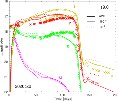
Figure 3: $ugri$ broad-band light curves (in apparent magnitudes) for selected directions of model s9.0 and SN 2020cxd (Yang et al., 2021).

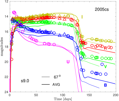
Figure 4: $U\!BV\!RI$ broad-band light curves (in apparent magnitudes) for selected directions of model s9.0 and SN 2005cs. The observational data for SN 2005cs are taken from Tsvetkov et al. (2006) (triangles) and from Pastorello et al. (2009) (circles).

3.2 Broad-band light curves compared to LL type IIP SNe

We present $U\!BV\!R$ broad-band light curves for all considered angular directions of our model s9.0 in Appendix C. In this section we show the results for a few selected angular directions suitable to reproduce the light curve properties of LL type IIP SNe 2020cxd and 2005cs (Figure 3 and Figure 4, respectively). In Figure 3, $ugri$ magnitudes for the 90^∘, 180^∘, and angle-averaged cases are shown together with those observed in SN 2020cxd. It is difficult to draw conclusions about the relevance of the synthetic light curves because of the limited set of filters used for the photometry of SN 2020cxd. However, the general behaviour of the fluxes in broad bands is explained by our selected cases. Specifically, the flux in the $g$-band is reproduced by the directions outside the main plume of s9.0 or the angle-averaged case to good agreement.

At the same time, the 66.7^∘, 67^∘, 90^∘, 180^∘, and angle-averaged models, match the general behaviour of the broad-band magnitudes of SN 2005cs (Pastorello et al., 2006; Tsvetkov et al., 2006; Pastorello et al., 2009), except during the first $\sim$50 days when the models underestimate the flux in all bands. However, the same is true for the comparison with the bolometric light curve of SN 2005cs as discussed in Section 3.1. We show only light curves for the 67^∘ and angle-averaged cases in Figure 4, since the rest of the suitable cases range between the 67^∘ and angle-averaged curves. We note that the results presented in this figure are from the new radiative-transfer simulations carried out on the basis of our updated profiles extracted from the 3D SN simulation of s9.0. There are only minor differences compared to the multi-band light curves published in Kozyreva et al. (2021) for the previously used initial profiles of this explosion model, but we include the figure here also to testify these slight differences. In Figure 16 (Appendix C), we additionally present the $B\!-\!V$ and $V\!-\!R$ colours for all considered radial directions of our 3D model s9.0 and compare them to the observed colours of SN 2005cs. The colour analysis shows that the overall trends of these observables of SN 2005cs are satisfactorily reproduced by the colour evolution of our model. During the first 50 days the rise of $V\!-\!R$ is somewhat better followed by the radial directions within the biggest plume ($0^{\circ}-10^{\circ}$), whereas the subsequent increase of $V\!-\!R$ at later times is close to that for the angle-averaged model and the radial directions outside of the main plume. In the case of $B\!-\!V$ the observational data are bracketed by the angle-averaged model and the large-angle directions on the one side and those for $0^{\circ}-10^{\circ}$ on the other side until about day 35. Subsequently, the data follow closely the evolution described by the angle-averaged model and the large-angle directions.

Nevertheless, we conclude that our angle-averaged model of s9.0 and the directions outside the main plume explain bolometric and broad-band light curves of the considered observational examples of the LL type IIP SN family sufficiently well. This is particularly noteworthy because we do not tune the output of the self-consistent 3D explosion simulations while mapping it into the radiative-transfer code STELLA except for adjusting the ⁵⁶Ni mass. We consider the good match between LL type IIP SN observations and our results for the light-curve modeling as a strong support for neutrino-driven explosion models of low-mass, low-energy SN explosions.

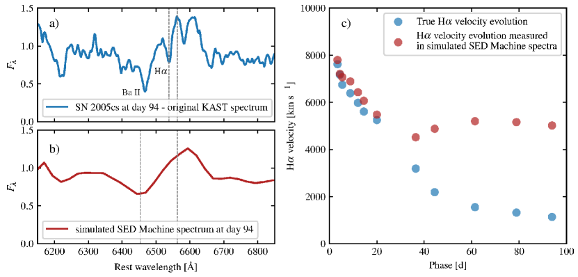
Figure 5: Demonstration of the effect of the spectral resolution on the measurement of line velocities. (a) Spectrum of SN 2005cs at 94 d (Faran et al., 2014); (b) its artificially degraded analogue mimicking the resolution of the P60 spectrograph, and (c) H$\alpha$ velocities deduced from the original spectra compared to those derived from their simulated low-resolution counterparts.

3.3 Photospheric velocity

One of the distinct observational features of LL type IIP SNe is the relatively low photospheric velocity during the plateau (Pignata, 2013; Spiro et al., 2014). A low photospheric velocity ($U_{\mathrm{ph}}$) or, more precisely, a low ratio between energy and ejecta mass (Tomasella et al., 2018), is the strongest diagnostic of low-energy explosions.

3.3.1 Line velocities in SNe 2020cxd and 2005cs

In observations, $U_{\mathrm{ph}}$ cannot be measured directly, but is usually approximated by measuring the velocity corresponding to the blueshift of the P-Cygni absorption lines. Dessart & Hillier (2005) have shown, based on synthetic spectra, that the so-derived velocities are good proxies for $U_{\mathrm{ph}}$ in the case of weak lines (such as Fe lines), but that with a strong line such as H$\alpha$, $U_{\mathrm{ph}}$ is often overestimated by up to 40 %.

For SN 2005cs, Pastorello et al. (2009) have measured H$\alpha$ and Sc ii velocities that are a factor of $\sim$2 lower than in normally luminous SNe II, declining from $\sim$7000 km s${}^{\,-1}$ in the earliest spectra to 1000–1500 km s${}^{\,-1}$ at the end of the plateau phase. The H$\alpha$ velocity evolution determined by Yang et al. (2021) blueand Valerin et al. (2022) for SN 2020cxd is surprisingly different from that of SN 2005cs, starting off at similar values a few days after the explosion, but declining only to $\sim$3000 km s${}^{\,-1}$ at the end of the plateau. However, these results have to be questioned for mainly two reasons:

1. For epochs later than 90–100 d, Yang et al. (2021) blueand Valerin et al. (2022) chose to measure the full width at half maximum (FWHM) of the H$\alpha$ emission line rather than the blueshift of the P-Cygni absorption. This renders it difficult to directly compare to values determined from absorption-line blueshifts. But even more, there is also a fundamental problem in the physical interpretation of these numbers. The FWHM of an emission line is a good indicator for the size of the emitting region in fully optically thin conditions, i.e., when no part of the emission is obscured by an optically thick inner core. However, the assumption of such conditions would automatically imply that $U_{\mathrm{ph}}=0$, meaning that FWHM measurements of emission lines are never a good way to measure $U_{\mathrm{ph}}$.

2. Several SN 2020cxd spectra of Yang et al. (2021) have been obtained with the SED Machine spectrograph on the Palomar 60-inch telescope. The SED Machine has a very low resolving power of $R=\frac{\lambda}{\Delta\lambda}\approx 100$ (Blagorodnova et al., 2018), corresponding to a velocity resolution of $\Delta v=c\,/\,R\approx 3000$ km s${}^{\,-1}$. This sets a lower limit for reliably measurable line blueshifts that is significantly higher than, e.g., the H$\alpha$ blueshifts of SN 2005cs towards the end of the plateau. Consequently, at least the H$\alpha$ velocity measurement of SN 2020cxd at day 94 ($\sim$3750 km s${}^{\,-1}$) appears dubious.

   To assess the possible effect of the SED Machine’s low resolution more quantitatively, we artificially degrade the resolution of a 94 d spectrum of SN 2005cs (Faran et al., 2014) to yield $R\approx 100$ by boxcar-smoothing it with a kernel of $\sim$65 Å and rebinning it to 25 Å bins. In Figure 5 we present the result of this procedure and demonstrate the corresponding effect of the low spectral resolution on estimating the photospheric expansion velocities via the H$\alpha$ line as in Yang et al. (2021). Panel (a) shows the spectrum of SN 2005cs taken 94 d after the explosion with the KAST spectrograph (Faran et al., 2014). The H$\alpha$ and Ba ii lines are rather narrow and well separated. A reliable H$\alpha$ velocity can be determined. Panel (b) displays the same spectrum, but artificially degraded to match the resolution of SED Machine ($R\sim 100$; Blagorodnova et al. 2018) at a bin width of 25 Å. The H$\alpha$ and Ba ii lines are fully blended, and the velocity inferred from the combined absorption trough is several times higher. Panel (c) presents a comparison between the temporal H$\alpha$ velocity evolution of SN 2005cs measured in the original spectra (Pastorello et al., 2009; Faran et al., 2014) and that determined from simulated spectra with SED Machine-like resolution.

   In the well-resolved original spectrum, for example, we measure an H$\alpha$ velocity of $\sim$1150 km s${}^{\,-1}$, in good agreement with the velocity evolution shown in Pastorello et al. (2009). In the smoothed spectrum, however, the H$\alpha$ line is completely blended with several Ba ii lines at slightly shorter wavelengths, and an attempt to measure the blueshift of the resulting trough yields an alleged H$\alpha$ velocity of $\sim$5100 km s${}^{\,-1}$. If the same Ba ii lines also contribute to the 94 d spectrum of SN 2020cxd, the reported H$\alpha$ velocity is likely to be overestimated by a factor of several.

In conclusion, the only line-velocity measurements of SN 2020cxd that can serve to estimate a photospheric velocity are those at $<$ 40 d after explosion, where either the spectra have sufficient resolution or the velocities are high enough that the low resolution of the SED Machine changes the result by at most a few hundred km s${}^{\,-1}$.

3.3.2 Modelled photospheric velocities

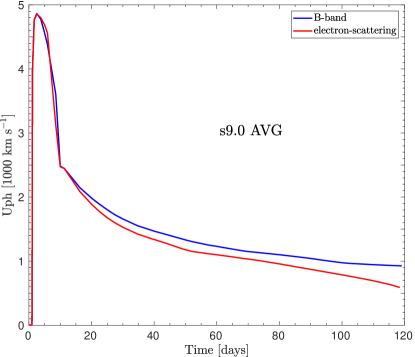
Figure 6: Synthetic photospheric velocity estimated via the integrated optical depth in the $B$ band (blue line) compared to that based on the electron-scattering opacity (red line). We use the angle-averaged case of s9.0 for demonstration.

The photospheric velocity in STELLA is estimated by default as the velocity of the shell where the integrated optical depth in the $B$-band is equal to 2/3. To back up this choice we compare it to the velocity at the location of the electron-scattering photosphere in the case of the angle-averaged explosion model in Figure 6. The integrated Thomson optical depth is computed with the total electron density provided by the Saha equation. In both cases the velocity is calculated at an optical depth equal to 2/3. Figure 6 confirms good agreement between the two approaches to estimate the photospheric velocities. The overall behavior is very similar but quantitative differences start at about day 15 and grow slowly with time. The photospheric velocity based on the electron-scattering opacity drops below the B-band value, however it is at most $\sim$20% smaller until day 100.

Figure 7 displays the $B$-band photospheric velocity evolution for our set of different radial directions from the asymmetric 3D explosion model s9.0. We superpose the data for the H$\alpha$ and Sc ii velocities of SN 2020cxd and SN 2005cs. We note that the photospheric velocities of SN 2005cs inferred from non-LTE steady-state modelling carried out with CMFGEN (Table 6 in Dessart et al., 2008) agree well with the observational data points shown in Figure 7 (grey and black symbols). The velocity evolution estimated via the observed H$\alpha$ line in SN 2020cxd (Yang et al., 2021; Valerin et al., 2022) as well as in SN 2005cs (Pastorello et al., 2009) is displayed after dividing the reported observational data by 1.4. This is considered as a proxy to the photospheric velocity, because Dessart & Hillier (2005) demonstrated that the H$\alpha$ velocity exceeds the photospheric velocity by a factor of up to 1.4. Nevertheless, even after dividing by 1.4, the H$\alpha$ velocity for SN 2020cxd remains too high compared to the values typically found for the family of LL type IIP SNe.

The photospheric velocity evolution for all explored radial directions is shown in Figure 7, because we presume that depending on the viewing direction of the SN, intrinsic, large-scale explosion asymmetries of low-mass iron-core progenitors as suggested by our explosion model s9.0 from Stockinger et al. (2020) may have some influence on the observed line velocities, in addition to their possible effects on the light curve discussed in Section 3.1. Therefore, since our analysis is based on 1D radiative transfer instead of full 3D transport calculations, it may be informative to consider the variation of the photospheric velocities in the different radial directions.

The spectral observations are sparse and under-resolved during the plateau phase of SN 2020cxd, as discussed in Section 3.3.1, which calls the information available for the photospheric velocity into question. Several spectra were taken with the SED Machine on the P60 telescope. The low spectral resolution of that spectrograph affects ejecta-velocity estimates. This is true for the velocities at day 2.4 and day 7.5, and especially at day 94.4, all of which are probably too high. Moreover, a comparison of the H$\alpha$ velocities to the photospheric velocity estimated in STELLA has to be taken with caution, because the synthetic-velocity estimate relies on the optical depth in the $B$ band and corresponds to the velocity measured via iron and scandium spectral lines, e.g., Fe ii 5169 Å or Sc ii 6246 Å. Assuming the H$\alpha$ velocity is correct and represents the location of the photosphere, the corresponding explosion energy of SN 2020cxd would be about 1.5 foe, which is very high even for a canonical type IIP SN. Assuming the H$\alpha$ velocity is two times higher than the realistic photospheric velocity (which may be too large a reduction), the explosion energy is still 0.5 foe, which corresponds to the average explosion energy of core-collapse SNe.

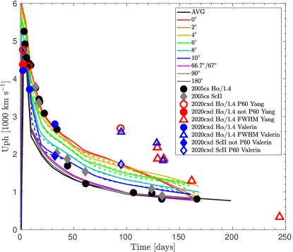
Figure 7: Time evolution of the photospheric velocity, U_ph, for different radial directions of model s9.0. The label “AVG” corresponds to the angle-averaged profile. The solid and dashed curves indicate the “$+$” and “$-$” directions for the cases of 2^∘–10^∘, as introduced in Table 2. The data points for SN 2005cs are taken from Pastorello et al. (2009). The red symbols represent data for SN 2020cxd taken from Yang et al. (2021) and the blue symbols represent data taken from Valerin et al. (2022). The H$\alpha$ velocity data are plotted after dividing by a factor of 1.4. The reliable data points are shown as filled symbols, whereas the open symbols represent less reliably measured velocities. See explanation in the text.

Nevertheless, the spectral lines remain quite narrow later, if we ignore the resolution constraints of the spectra, and at day 240 the measured intrinsic FWHM of the H$\alpha$ line is only 478 km s${}^{\,-1}$. Nebular spectral synthesis for the 1D version of model s9.0 displays narrow lines with FWHM about 1000 km s${}^{\,-1}$ at a similar epoch (Jerkstrand et al., 2018), corresponding to an explosion energy of 0.11 foe of the underlying 1D explosion model of s9.0 from Ertl et al. (2016) and Sukhbold et al. (2016). The very low velocity of SN 2020cxd at day 240 might be explained by an even lower explosion energy. Note that the 1D SN model of s9.0, which was exploded by a parametric treatment of the neutrino-heating mechanism (Ertl et al., 2016; Sukhbold et al., 2016), releases 0.11 foe, whereas the angle-averaged model of the self-consistent 3D neutrino-driven explosion simulation (Stockinger et al., 2020) has 0.07 foe. This corresponds to a factor of 0.8 in velocity, which is consistent with the observationally diagnosed ejecta velocity of SN 2020cxd after about 200 days to some extent.

None of the model results for the different angular directions of the 3D explosion of s9.0 can explain the photospheric velocity evolution of SN 2020cxd by itself. In fact, the H$\alpha$ velocities of SN 2020cxd around 100–150 days exceed the photospheric velocities of all model directions by far. Taking into account the discussion above and in the previous Section 3.3.1, we compare the synthetic velocities also to the more reliable data for the LL type IIP SN 2005cs. The photospheric velocity evolution of SN 2005cs is estimated via the Sc ii line (Pastorello et al., 2009). In contrast to SN 2020cxd, the line velocities of SN 2005cs are close to our computed results or overlap with them. During the plateau we can explain the photospheric velocity evolution of SN 2005cs with the velocities for the 8^∘ and 10^∘ directions, while at the end of the plateau and later our model directions for 66.7^∘, 67^∘, 90^∘, 180^∘, as well as the angle-averaged case match the observed values. However, we note that the photospheric-velocity estimates beyond the plateau phase are not perfectly reliable in the simulations carried out with STELLA, because STELLA is not capable to provide photospheric information when the SN ejecta become semi-transparent.

The fact that the evolution of the observationally diagnosed photospheric velocity of SN 2005cs agrees with the photosphere of our explosion model in different radial directions at different times during the plateau on the one hand and with the angle-averaged model at the end of the plateau on the other hand, might indicate some influence of explosion asymmetries on the line formation. This interpretation is compatible with our arguments for a possible impact of explosion asymmetries on the light curve of SN 2005cs discussed in Section 3.1. Such explosion asymmetries, which are suggested by the low-mass iron-core explosion model s9.0 of Stockinger et al. (2020), might play a role also in SN 2020cxd and other low-mass SN explosions. Unfortunately, no spectrapolarimetric observations have been carried out for SN 2020cxd. Pastorello et al. (2009) reported that SN 2005cs possesses asymmetric H$\alpha$ line shapes during the nebular phase with the emission maximum in the P-Cygni profiles shifted towards redder wavelengths by 700–800 km s${}^{\,-1}$. The latter might be explained by an asymmetric distribution of the radioactive material, i.e., by a dominant fraction of the ⁵⁶Ni in the inner part of the SN ejecta pointing away from the observer (Chugai, 2006). Moreover, Gnedin et al. (2007) presented imaging polarimetry of SN 2005cs and reported up to 8 % polarisation during the plateau phase. Such a high degree of polarisation would be unprecedented for Type II SNe (Leonard et al., 2002) and point at an asymmetry in the inner ejecta. However, the inspection of unpublished spectropolarimetric observations of SN 2005cs obtained with Keck + LRIS (Prog-ID C21L; PI: Leonard) does not seem to support the results by Gnedin et al. Another example of a LL type IIP SN with available spectrapolarimetric observations is SN 2008bk. The plateau luminosity of this SN is 0.4 dex higher than that of many LL type IIP SNe, whereas its photospheric velocities are comparable to those of other cases of the low-luminosity family (Pignata, 2013; Lisakov et al., 2018). The polarimetric behaviour during the plateau of SN 2008bk is pretty normal and inconspicuous, but after the drop from the plateau this SN retains a constant 0.3 % polarisation, which is unusual and might indicate some asymmetry inside the ejecta (Leonard et al., 2012). Therefore, although it is not possible to draw solid conclusions about explosion asymmetries on grounds of the existing data sets for SN 2005cs and SN 2020cxd, a possible role of such asymmetries in low-mass, low-energy, LL type IIP SNe can not be firmly excluded either. This stresses the need of more observational data to be compared with predictions for light curves, spectra, and polarisation based on 3D radiative transfer calculations in 3D explosion models.

3.4 Testing the SN progenitor model by Yang et al. 2021

In order to test the SN properties deduced by Yang et al. (2021), we construct two models which we map into STELLA.

The first case is based on model m12 from Kozyreva et al. (2019), which has almost the proposed ejecta mass. Namely, m12 has 11.25 $\mathrm{M}_{\odot}$ at the pre-collapse stage. Accounting for a mass of 1.45 $\mathrm{M}_{\odot}$ for the newly-formed compact object results in 9.8 $\mathrm{M}_{\odot}$ for the SN ejecta. To match the proposed value of 9.5 $\mathrm{M}_{\odot}$, we scale the density profile with the factor of 9.5/9.8. The radius of the progenitor is 496 $\mathrm{R}_{\odot}$. To transform this radius to the required value of 187 $\mathrm{R}_{\odot}$, we squeeze each mass zone in the mapped model with a compression factor of 187/496, conserving the mass contained in the zone. We note that model m12 was exploded with the V1D code (Livne, 1993) with an original explosion energy of 0.9 foe. We scale the velocity profile to change this explosion energy to a value of 0.58 foe. The total mass of ⁵⁶Ni is scaled to the value of 0.003 $\mathrm{M}_{\odot}$ for SN 2020cxd. The difference in the ⁵⁶Ni mass fraction is added to the silicon abundance.

The second model is based on model s12 from Sukhbold et al. (2016), which was evolved with the stellar evolution code KEPLER until the pre-collapse state. Later, after the necessary modifications, we map the model into STELLA and blow it up with the thermal-bomb method, in which a prescribed amount of thermal energy is injected at the inner boundary (i.e., the mass coordinate corresponding to the assumed mass of the compact remnant of 1.35 $\mathrm{M}_{\odot}$) within a mass shell of 0.06 $\mathrm{M}_{\odot}$. The total pre-collapse mass of this progenitor is 10.95 $\mathrm{M}_{\odot}$. After subtracting 1.35 $\mathrm{M}_{\odot}$ for the compact object, the ejecta mass is 9.55 $\mathrm{M}_{\odot}$, which is very close to the 9.5 $\mathrm{M}_{\odot}$ value of the analysis by Yang et al. (2021). The radius of s12 prior to collapse is 613 $\mathrm{R}_{\odot}$. To make the model more compact, we follow the same procedure as described for model m12 above. The injected thermal-bomb energy is set to 1.73 foe, which leads to a terminal kinetic energy of 0.58 foe. We note that these are two different models, computed with different stellar evolution codes. Nevertheless, their chemical structures are very similar, particularly in the hydrogen-rich envelope, which reflects the typical structure of red supergiants and is much more extended than the radius inferred by Yang et al. (2021).

The resulting light curves for the re-scaled m12_scale and s12_scale models are shown in Figure 8. It is evident that despite m12 and s12 being two different stellar models, exploding them with the same explosion energy after scaling their characteristic progenitor parameters to the same values leads to almost the same bolometric light curves. The explosion energy of 0.58 foe has a distinctive effect on the bolometric luminosity and duration of the plateau. The difference in the light curves at early times is connected to slightly different density structures in the outermost layers of the stellar envelopes. The difference in the light curves at the beginning of the radioactive tail is connected to the numerical viscosity and the zoning in the innermost parts of the ejecta. The plateau of both models lasts only about 80 days versus the 130-day plateau of SN 2020cxd, and has a bolometric magnitude of $\,-15.5$ mag, which is 1.5 mag higher than that of SN 2020cxd.

The photospheric velocities are around 2780 km s${}^{\,-1}$ for both models in the middle of their bolometric plateaus, i.e. around day 40. We note that this value is close to the 2747 km s${}^{\,-1}$ reported by Yang et al. (2021) as the expansion velocity of their best-fit model found by the MCMC light curve fitting procedure. This agreement is a consequence of the fact that we set the explosion energy of our models equal to the value inferred by those authors.

With this experiment we show that LL Type IIP SNe, particularly SN 2020cxd, cannot be explained with the progenitor and SN parameters derived by the analysis of Yang et al. (2021).

Figure 8: Bolometric light curves for our two explosion models s12_scale and m12_scale with progenitor and explosion properties adjusted to those inferred by Yang et al. (2021).

3.5 Is SN 2020cxd an ECSN?

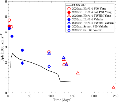
Figure 9: Left: $gri$ broad-band light curves for the ECSN model from Kozyreva et al. (2021) and SN 2020cxd. Right: Photospheric velocity evolution for the ECSN model and SN 2020cxd. The observational data are the same as in Figure 3 and Figure 7.

According to a number of studies, LL type IIP SNe might be interpreted as electron-capture SNe (ECSNe, Botticella et al., 2009; Pumo et al., 2009; Cai et al., 2021; Reguitti et al., 2021; Valerin et al., 2022). One of the reasons for this interpretation are identifications of progenitors as low-mass stars with a ZAMS mass around 8 $\mathrm{M}_{\odot}$, embedded in some cases in a dusty environment. However, we note that progenitor mass estimates are strongly model dependent with a number of caveats.

In Figure 9 we show the broad-band magnitudes for SN 2020cxd and for an ECSN model (e8.8) published in Kozyreva et al. (2021) to test this hypothesis. The progenitor of the ECSN considered in that study has an extended and very tenuous hydrogen-rich envelope. The density and chemical structure of the progenitor are believed to be representative of this kind of massive stars, namely, massive asymptotic giant branch stars. The extended envelope is the result of a sequence of flashes happening during the helium-core burning (Jones et al., 2013, 2014; Jones et al., 2016). The resulting light curves are far too luminous to be LL type IIP cases, and Kozyreva et al. (2021) concluded that the characteristic luminosities of ECSNe are comparable to those of reference cases of SNe IIP. Moreover, ECSNe have a very distinct colour evolution. In particular, the $U$-band magnitude has a plateau at $-15.5$ mag during the first 60 days, which is very different from the behaviour of the $U$-band light curve of typical type IIP SNe. The unique $U$-band light curves of ECSNe are explained by the fact that recombination in their envelopes sets in relatively late around day 70. We also superpose the photospheric velocity evolution for our ECSN model e8.8 and the velocities of SN 2020cxd (right plot in Figure 9). The observed H$\alpha$ velocities (after dividing by 1.4) are roughly 1000 km s${}^{\,-1}$ higher than those predicted by the ECSN model at an early epoch when the SN 2020cxd velocity estimates are still reliable, although the Sc II line velocity estimated at day 32 is consistent with the ECSN.

4 Summary and conclusions

In this study we compared the observational data of the LL type IIP SNe 2020cxd and 2005cs with multi-band light curves and photospheric velocities obtained from radiation-hydrodynamics calculations for a 3D explosion model of a 9.0 M_⊙ (ZAMS mass) red supergiant progenitor with an iron core of 1.3 M_⊙ and a radius of 408 $\mathrm{R}_{\odot}$ (Woosley & Heger, 2015). The stellar model had a pre-collapse mass of 8.75 M_⊙ (an ejecta mass of 7.4 $\mathrm{M}_{\odot}$) and was self-consistently exploded by the neutrino-driven mechanism in a 3D simulation by Stockinger et al. (2020). The model had developed a considerable asphericity by hydrodynamic instabilities aiding the onset of the explosion. These initial asymmetries ultimately evolved into large-scale asymmetries in the angular distribution of ⁵⁶Ni, connected to extended radial mixing of metals from the core into the hydrogen-helium envelope. This mixing proceeded in the form of elongated wide-angle plumes, which led to a prolate global deformation of the chemical composition in the ejecta (see Figure 1 and for details, see Stockinger et al. 2020).

The subsequent long-time SN evolution, starting from the 3D explosion model at 1.974 days after core bounce, was carried out by spherically symmetric hydrodynamical simulations with the STELLA code, including multi-band radiative transfer. For that we considered the spherically averaged 3D model as well as the conditions in selected radial directions with a different extent of outward metal mixing, covering big ⁵⁶Ni plumes as well as regions of less efficient mixing. Performing radiative transfer calculations with the sphericized stellar profiles for these selected directions was intended to demonstrate the possible relevance of asymmetry effects in the radiation emission of the 3D explosion model. Aspherical radiation transport can, of course, be reliably treated only by 3D radiative transfer calculations in the 3D SN ejecta, whereas our approach tends to massively overestimate the influence of direction-dependent variations in the density structure and chemical composition. But nevertheless, our calculations might demonstrate the basic trends that could be associated with the existence of such large-scale chemical and density anisotropies in a fully multi-dimensional radiative transfer treatment.

We found that our neutrino-driven explosion model of the 9 M_⊙ progenitor with an explosion energy of 0.07 foe and an ejecta mass of 7.4 M_⊙ can amazingly well reproduce the basic properties of the bolometric light curve of SN 2020cxd, i.e., its initial decline to the plateau, the height and duration of the plateau, and the shallow increase of the plateau luminosity until the steep decline to the radioactive-decay tail. This is achieved without any fine tuning of the explosion model except for a proper scaling of the ⁵⁶Ni mass to the observationally inferred value of 0.003 M_⊙ for SN 2020cxd. Such a scaling is motivated by considerable modeling uncertainties with respect to an exact determination of the ⁵⁶Ni yield. Good overall agreement was also obtained for the broad-band light curves of this SN. In contrast, however, the line velocities reported by Yang et al. (2021) do not mirror the time evolution of the photospheric expansion velocities deduced from our radiative transfer calculations but are considerably higher (up to a factor of $\sim$3) than the model values. This holds true even in the directions of the fastest ejecta expansion connected to the most extended nickel-rich plume, and even after scaling down the measured H$\alpha$ line velocities by a factor of 1.4 as recommended by Dessart & Hillier (2005) for comparison with the photospheric velocities from radiative transfer modeling.

This is in stark contrast to our findings for SN 2005cs, which is a template case of a low-energy, LL type IIP SN with low ⁵⁶Ni production. Here not only the bolometric and broad-band light curves match the observational ones reasonably well, again without any other tuning than scaling the ⁵⁶Ni mass. Also the photospheric velocities are close to the velocities of the Sc ii line and the down-scaled H$\alpha$ line of SN 2005cs and follow their evolutionary behavior.

We speculated whether the different shapes of the light curves of SN 2005cs and SN 2020cxd during the initial decline to the plateau and the early plateau phase might be connected to large-scale ejecta asymmetries already at shock breakout and during the early expansion of the outer parts of the hydrogen envelope. Such a possibility is suggested by our 3D explosion model of the 9 M_⊙ progenitor, which exhibits large-scale asymmetries of the nickel-rich ejecta, which extend through the entire hydrogen envelope and lead to asymmetric shock breakout (see Stockinger et al. 2020 and Figure 1). Contributions by radiation emitted from the faster and more rapidly expanding directions of the ejecta might enhance the luminosity of SN 2005cs before and during the plateau until about 80–90 days, whereas in SN 2020cxd such effects might not play an important role or they might not be visible from our viewing direction. Interestingly, we also witnessed the trend that at early phases the line velocities of SN 2005cs were best compatible with the photospheric velocities in the directions of the fastest ejecta in our aspherical 3D explosion model, whereas with progressing time they approached those of the ejecta in directions with slower expansion, and, at late times, they agreed with those of the angle-averaged ejecta. This might also be interpreted as a possible indication of large-scale or even global explosion asymmetries in the outer ejecta of SN 2005cs, adding to similar conclusions previously drawn by Pastorello et al. (2009), Chugai (2006), and Gnedin et al. (2007) on grounds of asymmetric H$\alpha$ line shapes and polarisation measurements. A better theoretical understanding of whether such a speculative possibility can explain the light-curve differences of SN 2005cs and SN 2020cxd and the evolution of their line velocities will require 3D radiative transfer calculations for our 3D explosion model or other simulations of asymmetric SNe of low-mass progenitors.

In both of the cases of SN 2020cxd and SN 2005cs, a very low-energy explosion of our low-mass iron-core progenitor can explain the main light-curve features. We reason that the similarities between the photospheric velocities of our model and the line velocities for SN 2005cs and their mismatch in the case of SN 2020cxd point to a considerable overestimation of the observationally inferred line velocities in the latter case. We discussed the corresponding instrumental and diagnostic uncertainties. Both SNe, therefore, seem to comply with the correlation between explosion energy and ejected mass of ⁵⁶Ni inferred from Type IIP SN observations (Pejcha & Prieto, 2015b; Müller et al., 2017b; Pejcha, 2020) and theoretically expected for neutrino-driven explosions (Ertl et al., 2016; Müller et al., 2016; Sukhbold et al., 2016; Ertl et al., 2020).

A striking difference is observed when comparing the explosion energy of our explosion and light-curve model, 0.07 foe, to the explosion energies of LL type IIP SNe derived with the use of the so-called Markov Chain Monte Carlo (MCMC) fitting method (Nagy & Vinkó, 2016). For example, SN 2020cxd was reported to have a total energy of 0.58 foe (Yang et al., 2021), SN 2005cs to have a sum of kinetic and thermal energy of 0.73 foe, and its declared twin PSN J17292918+7542390 (SN-NGC 6412, Jäger et al., 2020) to have an even higher explosion energy of 0.82–0.93 foe. Using the same method, the reference Type IIP SN 1999em was diagnosed to originate from the explosion of a progenitor of about 20 $\mathrm{M}_{\odot}$ (the ejecta mass was estimated to be 19 $\mathrm{M}_{\odot}$) with a diagnostic energy of 4.53 foe. At the same time the recent progress in self-consistent core-collapse explosion simulations coupled with direct radiative transfer hydrodynamics calculations for the light curve has been able to reproduce this SN 1999em by an explosion of a 15 $\mathrm{M}_{\odot}$ progenitor with an energy of 0.55 foe (Utrobin et al., 2017). Hence, there is a factor of 10 difference in the derived SN parameters. The MCMC fitting procedure is likely to suffer from various weak points, among them might be a relatively high lower limit for the explosion energy of 0.6 foe (Hamuy, 2003) and a simplified method for computing the bolometric light curve (Arnett & Fu, 1989; Popov, 1993; Nagy et al., 2014). However, the details of the statistical analysis are not fully described in the mentioned references, which complicates any assessment of the employed fitting procedure and results in detail.

Data availability

The light-curve data computed and analysed for the current study are available via the link https://wwwmpa.mpa-garching.mpg.de/ccsnarchive/data/Kozyreva2022/. Angle-averaged data of the 3D core-collapse SN simulation by Stockinger et al. (2020) and the radial profiles along the selected angular directions used in the present work are accessible for download at https://wwwmpa.mpa-garching.mpg.de/ccsnarchive/data/Stockinger2020/.

Software

PROMETHEUS-VERTEX (Fryxell et al., 1989; Rampp & Janka, 2002; Buras et al., 2006); PROMETHEUS-HOTB (Kifonidis et al., 2003; Scheck et al., 2006; Arcones et al., 2007; Ertl et al., 2016) NUMPY and SCIPY (Jones et al., 2001); IPYTHON (Perez & Granger, 2007); MATPLOTLIB (Hunter, 2007); VisIt (Childs et al., 2012); STELLA (Blinnikov et al., 1998, 2000, 2006); IRAF (Tody, 1986).

Appendix A Profiles of the angle-averaged explosion-model data used in Kozyreva et al. (2021) and in the present study

We show the employed initial profiles of the angle-averaged velocity, density, and ⁵⁶Ni mass fraction versus radius (Figure 10) and enclosed mass (Figure 11) compared to the profiles used in Kozyreva et al. (2021). Instead of considering model results from Stockinger et al. (2020) at 2.82 days after the onset of the explosion as in the previous work, we started the radiation-hydrodynamic light-curve modeling in the present study with a model profile at 1.97 days, which is about 0.2 days before the fastest part of the highly deformed SN shock breaks out from the progenitor surface. This ensures a somewhat cleaner modeling of the shock-breakout phase in our 1D simulations, because this phase takes roughly 1 day in the non-spherical 3D explosion model of Stockinger et al. (2020), leading to a corresponding broadening of the structural features near the stellar surface.

Besides a somewhat smaller shock radius, the earlier initial profile of the present study displays an outward going wave around a radius of $6\times 10^{12}$ cm and enclosed mass of 1.4 M_⊙ visible as velocity bump in the red lines. This feature is connected to the reflection of the reverse shock near the stellar center and has moved to a larger radius and enclosed mass in the later simulation output ($\sim$ $1.2\times 10^{13}$ cm and $\sim$1.7 M_⊙, respectively). The extreme deformation of the pre-breakout shock in the 3D explosion model at 1.97 days is clearly obvious from the fact that the corresponding velocity jump in the angle-averaged profile is smeared over a mass interval between 6.6 M_⊙ and 8.6 M_⊙. The local maximum in the profile of the ⁵⁶Ni mass fraction at radii $>$ $2\times 10^{13}$ cm (enclosed mass between $\sim$6.6 M_⊙ and $\sim$8.5 M_⊙) is connected to the biggest low-mass high-velocity nickel-rich plume prominently visible in Figure 1.

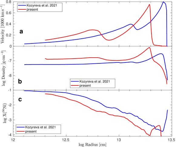
Figure 10: Velocity (a), density (b) and ⁵⁶Ni mass fraction (c) of the angle-averaged profiles used in the present study and in Kozyreva et al. (2021) along the radius coordinate. The red lines correspond to the profiles at 1.97 days after the onset of the explosion and the blue lines to the profiles at 2.82 days.

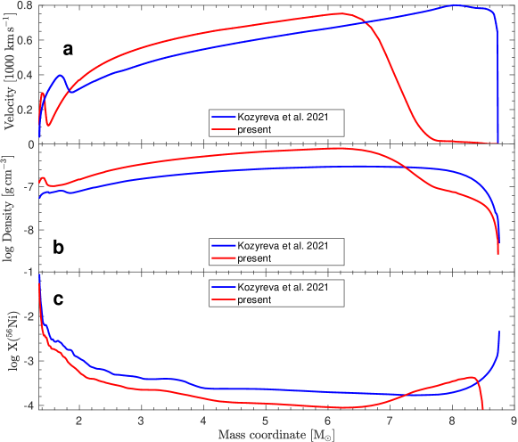
Figure 11: Velocity (a), density (b) and ⁵⁶Ni mass fraction (c) of the angle-averaged profiles used in the present study and in Kozyreva et al. (2021) along the mass coordinate. The red lines correspond to the profiles at 1.97 days after the onset of the explosion and the blue lines to the profiles at 2.82 days.

Appendix B Angle-averaged and radial-direction dependent profiles extracted from the 3D supernova explosion simulation

Figure 12, Figure 13, and Figure 14 display the profiles of velocity, density, and ⁵⁶Ni mass fraction, respectively, of all selected radial directions of model s9.0 that were used as initial data for our radiation-hydrodynamics simulations in the present study. At the given time of 1.97 days after core collapse the shock wave in the fastest moving parts of the SN ejecta is within about $3\times 10^{12}$ cm from the stellar surface and breaks out within $\sim$0.2 days. It corresponds to the great, low-mass nickel-rich plume subtending the directions from $0^{\circ}$ to about $10^{\circ}$ in Figure 1. The shock wave in the slowest parts of the ejecta is still about $10^{13}$ cm away from the stellar edge and will reach the surface roughly 1 day after the fastest regions of the shock. In the angle-averaged velocity profile (bold black solid line) the fast-moving ⁵⁶Ni plume is hardly visible because of the small angular extension of this feature.

Similarly, the biggest plume forms a prominent cusp in the density profile around $\sim$ $2.5\times 10^{13}$ cm (mass coordinate around 8.4 M_⊙ for directions between 0^∘ and 10^∘, which moves well ahead of the main shock and the main ejecta shell with its density maximum at about $2\times 10^{13}$ cm. This main ejecta shell appears as a broad dome from $\sim$2 M_⊙ to $\sim$7.5 M_⊙ in the density profile versus enclosed mass (Figure 13). Again, the angle-averaged profile (bold black solid line) does not carry any evidence of the fastest, most elongated nickel plume because of the small amount of mass in this structure. The lower-amplitude density and velocity fluctuations at small radii and enclosed masses correspond to waves and density inhomogeneities in the inner, slow ejecta.

In the ⁵⁶Ni distribution (Figure 14) high mass fractions signal the existence of a more spherical bulk mass of slower nickel that extends up to $\sim$10¹³ cm and has low expansion velocities ($\lesssim$500 km s^-1; see lines for 90^∘ and 180^∘ directions and also Figure 1). Moreover, besides the biggest nickel-rich plume (directions 0^∘ to $\sim$10^∘) high ⁵⁶Ni concentrations can be found in secondary plumes reaching up to around $1.3\times 10^{13}$ cm and thus overlapping with the innermost parts of the dense main ejecta shell (66.7^∘ and 67^∘ directions).

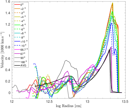
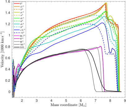
Figure 12: Velocity of the angle-averaged profile (“AVG”) and different radial directions of the model s9.0 used in the present study along the radius coordinate (left) and the mass coordinate (right).

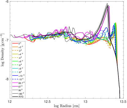
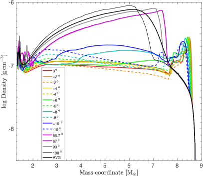
Figure 13: Density of the angle-averaged profile (“AVG”) and different radial directions of the model s9.0 used in the present study along the radius coordinate (left) and the mass coordinate (right).

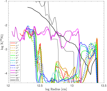
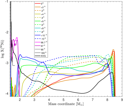
Figure 14: ⁵⁶Ni mass fraction of the angle-averaged profile (“AVG”) and different radial directions of the model s9.0 used in the present study along the radius coordinate (left) and the mass coordinate (right).

Appendix C Broad-band light curves and colours for all radial directions in the present study

We present the $U\!BV\!R$ broad-band magnitudes for all radial directions considered in our study and the angle-averaged profile of model s9.0 in Figure 15. The broad-band light curves behave similarly to the bolometric light curves and reflect the properties of the profiles for the different considered radial directions. In the radial directions aligned with the main nickel-rich plume, i.e., for 0^∘, 2^∘, 4^∘, 6^∘, 8^∘, and 10^∘, radioactive nickel is distributed such that a relatively large fraction of it is located close to the stellar surface because of the deep penetration of the plume into the hydrogen envelope (see Figure 14). Moreover, the density distribution in these radial directions indicates lower density along the main plume than in its surroundings (see Figure 13). Therefore the $4\pi$-equivalent of the total mass that is relevant when the data are sphericized and mapped into the 1D treatment with STELLA is relatively low compared to the radial directions outside of the main plume and the angle-averaged profile (see Table 2). For example, the effective ejecta mass for the 0^∘ direction is only 4.4 $\mathrm{M}_{\odot}$. Note, however, that the stellar radii for all radial directions are the same. Since the bulk velocity of the matter in the main plume is higher than that along the radial directions outside of it (see Figure 12), the effective explosion energy after spherisation reaches $\sim$0.13 foe, whereas the $4\pi$-equivalent values of the explosion energies for the $66.7^{\circ}\!-\!180^{\circ}$ directions are only 0.07–0.08 foe.

Consequently, in the radial directions away from the high-entropy plume the light curve shapes of all broad bands are comparable to those of characteristic SNe IIP, even though they reach lower luminosities because of the lower explosion energies than canonical type II SNe. In contrast, all radial directions along the main plume represent high-energy explosions with low-mass ejecta. Their light curves are shorter and possess higher luminosities, and their $U$-band magnitudes are higher than that of the angle-averaged case, because the plume contains hotter material. We note that the amount of ⁵⁶Ni is scaled to 0.003 $\mathrm{M}_{\odot}$, for which reason the light curves for all radial directions including those inside the main plume are not powered by ⁵⁶Ni decay but by recombination. The light curves for all of the radial directions within $0^{\circ}\!-\!10^{\circ}$ exhibit a knee around day 40–50, when recombination sets in in the ejecta. A similar behaviour is observed in the ECSN model e8.8 published by Kozyreva et al. (2021); especially the $U$-band magnitude of this model exhibits a gentle rise of the plateau until about day 50. In the case of the ECSN model this long period of time until recombination starts is explained by the large progenitor radius. In the cases of the radial directions along the main plume of our s9.0 model, the reason for the delayed recombination is the relatively hotter material in this plume.

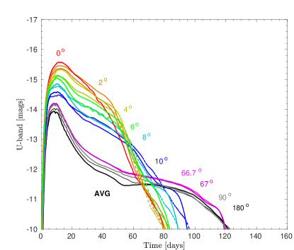
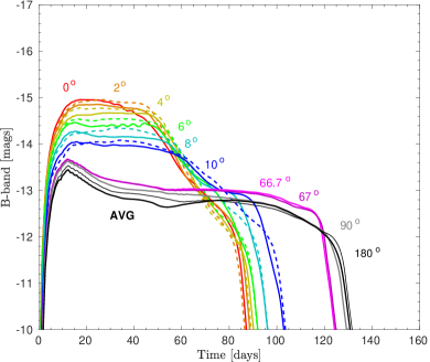
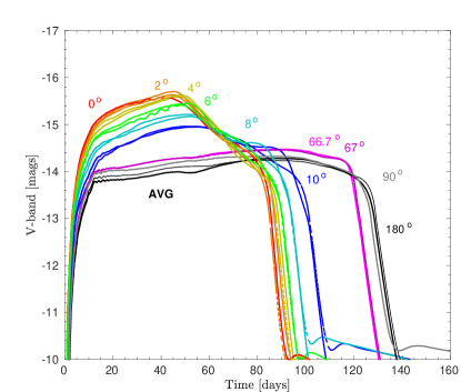
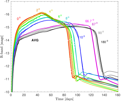
Figure 15: $U\!BV\!R$ broad-band light curves for the angle-averaged profile (“AVG”) and different radial directions of the 3D model s9.0. The solid and dashed curves indicate the “$+$” and “$-$” directions for the cases of 2^∘–10^∘, as introduced in Table 2.

In Figure 16, we present the $B\!-\!V$ and $V\!-\!R$ colour evolution for all considered radial directions of our 3D model s9.0 with the data for SN 2005cs superposed. Kozyreva et al. (2019) pointed out that the $B\!-\!V$ colour may serve as a diagnostic parameter for the macroscopic mixing processes that take place in the SN ejecta after the passage of the shock wave [the interested reader is referred to a discussion of this hydrodynamical phenomenon in recent 3D explosion models of type IIP SNe by Wongwathanarat et al. (2015) and Utrobin et al. (2017)]. The colours indicate the temperature of the SED and indirectly reflect the degree of absorption in the SN ejecta. Since iron-group elements are the main contributors to the line opacity, their distribution determines how red or blue the SN spectra are. Therefore, the colours are blue, i.e., $B\!-\!V$ is close to 0, during the early time when the photosphere is still far from the iron-rich interior of the SN ejecta. Later, at the end of the plateau, $B\!-\!V$ approaches 2–3 mag, indicating significant redistribution of the flux between the spectral bands caused by the higher fraction of iron-group elements in the inner part of the ejecta.

During the first 50 days the $B\!-\!V$ and $V\!-\!R$ colours for the radial directions between $0^{\circ}$ and $10^{\circ}$ remain slightly ($0.2-0.3$ mags) bluer than those for the directions outside of the main plume, because the ejecta within the plume are less massive and carry a higher energy (see Table 2), for which reason the resulting radiation is hotter.

The comparison to SN 2005cs reveals that our explosion model can nicely reproduce the overall evolution of the observational data. In the time interval between about day 10 and day 30–50, there is a slight tendency that the observations are matched better by the colours for the radial directions within $0^{\circ}\!-\!10^{\circ}$, whereas at later times the observations closely follow the colour evolution for the angle-averaged case as well as for the radial directions at $66.7^{\circ}$, $67^{\circ}$, $90^{\circ}$, and $180^{\circ}$. These findings are in line with the trends we witnessed for our synthetic bolometric light curves compared to SN 2005cs in Figure 2, and for our theoretical photospheric velocities in comparison to the data of SN 2005cs in Figure 7.

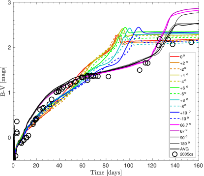
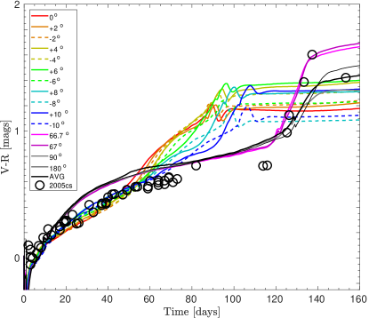
Figure 16: $B\!-\!V$ and $V\!-\!R$ colour evolution for all considered radial directions in comparison to SN 2005cs. The observational data for SN 2005cs (circles) are taken from Pastorello et al. (2009).

References

- Arcones et al. (2007) Arcones A., Janka H. T., Scheck L., 2007, A&A, 467, 1227
- Arnett (1980) Arnett W. D., 1980, ApJ, 237, 541
- Arnett & Fu (1989) Arnett W. D., Fu A., 1989, ApJ, 340, 396
- Blagorodnova et al. (2018) Blagorodnova N., et al., 2018, PASP, 130, 035003
- Blinnikov et al. (1998) Blinnikov S. I., Eastman R., Bartunov O. S., Popolitov V. A., Woosley S. E., 1998, ApJ, 496, 454
- Blinnikov et al. (2000) Blinnikov S., Lundqvist P., Bartunov O., Nomoto K., Iwamoto K., 2000, ApJ, 532, 1132
- Blinnikov et al. (2006) Blinnikov S. I., Röpke F. K., Sorokina E. I., Gieseler M., Reinecke M., Travaglio C., Hillebrandt W., Stritzinger M., 2006, A&A, 453, 229
- Bollig et al. (2021) Bollig R., Yadav N., Kresse D., Janka H.-T., Müller B., Heger A., 2021, ApJ, 915, 28
- Botticella et al. (2009) Botticella M. T., et al., 2009, MNRAS, 398, 1041
- Buras et al. (2006) Buras R., Rampp M., Janka H. T., Kifonidis K., 2006, A&A, 447, 1049
- Burrows et al. (2019) Burrows A., Radice D., Vartanyan D., 2019, MNRAS, 485, 3153
- Cai et al. (2021) Cai Y. Z., et al., 2021, A&A, 654, A157
- Caputo et al. (2022a) Caputo A., Janka H.-T., Raffelt G., Vitagliano E., 2022a, arXiv e-prints, p. arXiv:2201.09890
- Caputo et al. (2022b) Caputo A., Raffelt G., Vitagliano E., 2022b, Phys. Rev. D, 105, 035022
- Carenza et al. (2019) Carenza P., Fischer T., Giannotti M., Guo G., Martínez-Pinedo G., Mirizzi A., 2019, J. Cosmology Astropart. Phys., 2019, 016
- Chang et al. (2018) Chang J. H., Essig R., McDermott S. D., 2018, Journal of High Energy Physics, 2018, 51
- Childs et al. (2012) Childs H., et al., 2012, in Wes Bethel E., Childs H., Hansen C., eds, High Performance Visualization–Enabling Extreme-Scale Scientific Insight. Boca Raton, FL: CRC Press, pp 357–372
- Chugai (2006) Chugai N. N., 2006, Astronomy Letters, 32, 739
- Dessart & Hillier (2005) Dessart L., Hillier D. J., 2005, A&A, 439, 671
- Dessart et al. (2008) Dessart L., et al., 2008, ApJ, 675, 644
- Ertl et al. (2016) Ertl T., Janka H. T., Woosley S. E., Sukhbold T., Ugliano M., 2016, ApJ, 818, 124
- Ertl et al. (2020) Ertl T., Woosley S. E., Sukhbold T., Janka H. T., 2020, ApJ, 890, 51
- Faran et al. (2014) Faran T., et al., 2014, MNRAS, 442, 844
- Fryxell et al. (1989) Fryxell B., Müller E., Arnett D., 1989, in Hillebrandt W., Müller E., eds, Nuclear Astrophysics.
- Glas et al. (2019) Glas R., Just O., Janka H. T., Obergaulinger M., 2019, ApJ, 873, 45
- Gnedin et al. (2007) Gnedin Y. N., Larionov V. M., Konstantinova T. S., Kopatskaya E. N., 2007, Astronomy Letters, 33, 736
- Goldberg et al. (2019) Goldberg J. A., Bildsten L., Paxton B., 2019, ApJ, 879, 3
- Grasberg & Nadezhin (1976) Grasberg E. K., Nadezhin D. K., 1976, Ap&SS, 44, 409
- Hamuy (2003) Hamuy M., 2003, ApJ, 582, 905
- Hunter (2007) Hunter J. D., 2007, Computing in Science and Engineering, 9, 90
- Jäger et al. (2020) Jäger Zoltán J., et al., 2020, MNRAS, 496, 3725
- Janka (2017) Janka H.-T., 2017, in Alsabti A. W., Murdin P., eds, , Handbook of Supernovae. Cham, Switzerland: Springer Nature, p. 1095, doi:10.1007/978-3-319-21846-5_109
- Jerkstrand et al. (2018) Jerkstrand A., Ertl T., Janka H. T., Müller E., Sukhbold T., Woosley S. E., 2018, MNRAS, 475, 277
- Jones et al. (2001) Jones E., Oliphant T., Peterson P., et al., 2001, SciPy: Open source scientific tools for Python, http://www.scipy.org/
- Jones et al. (2013) Jones S., et al., 2013, ApJ, 772, 150
- Jones et al. (2014) Jones S., Hirschi R., Nomoto K., 2014, ApJ, 797, 83
- Jones et al. (2016) Jones S., Röpke F. K., Pakmor R., Seitenzahl I. R., Ohlmann S. T., Edelmann P. V. F., 2016, A&A, 593, A72
- Kasen & Woosley (2009) Kasen D., Woosley S. E., 2009, ApJ, 703, 2205
- Kifonidis et al. (2003) Kifonidis K., Plewa T., Janka H. T., Müller E., 2003, A&A, 408, 621
- Kozyreva et al. (2019) Kozyreva A., Nakar E., Waldman R., 2019, MNRAS, 483, 1211
- Kozyreva et al. (2020) Kozyreva A., Shingles L., Mironov A., Baklanov P., Blinnikov S., 2020, MNRAS, 499, 4312
- Kozyreva et al. (2021) Kozyreva A., Baklanov P., Jones S., Stockinger G., Janka H.-T., 2021, MNRAS, 503, 797
- Lentz et al. (2015) Lentz E. J., et al., 2015, ApJ, 807, L31
- Leonard et al. (2002) Leonard D. C., Filippenko A. V., Chornock R., Li W., 2002, AJ, 124, 2506
- Leonard et al. (2012) Leonard D. C., Dessart L., Hillier D. J., Pignata G., 2012, in Hoffman J. L., Bjorkman J., Whitney B., eds, American Institute of Physics Conference Series Vol. 1429, Stellar Polarimetry: from Birth to Death. pp 204–207 (arXiv:1109.5406), doi:10.1063/1.3701926
- Levesque et al. (2005) Levesque E. M., Massey P., Olsen K. A. G., Plez B., Josselin E., Maeder A., Meynet G., 2005, ApJ, 628, 973
- Levesque et al. (2006) Levesque E. M., Massey P., Olsen K. A. G., Plez B., Meynet G., Maeder A., 2006, ApJ, 645, 1102
- Lisakov et al. (2018) Lisakov S. M., Dessart L., Hillier D. J., Waldman R., Livne E., 2018, MNRAS, 473, 3863
- Livne (1993) Livne E., 1993, ApJ, 412, 634
- Mattila et al. (2008) Mattila S., Smartt S. J., Eldridge J. J., Maund J. R., Crockett R. M., Danziger I. J., 2008, ApJ, 688, L91
- Melson et al. (2015a) Melson T., Janka H.-T., Marek A., 2015a, ApJ, 801, L24
- Melson et al. (2015b) Melson T., Janka H.-T., Bollig R., Hanke F., Marek A., Müller B., 2015b, ApJ, 808, L42
- Melson et al. (2020) Melson T., Kresse D., Janka H.-T., 2020, ApJ, 891, 27
- Mori et al. (2022) Mori K., Takiwaki T., Kotake K., Horiuchi S., 2022, Physical Review D, 105, 063009
- Moriya et al. (2020) Moriya T. J., Suzuki A., Takiwaki T., Pan Y.-C., Blinnikov S. I., 2020, MNRAS, 497, 1619
- Müller et al. (2016) Müller B., Heger A., Liptai D., Cameron J. B., 2016, MNRAS, 460, 742
- Müller et al. (2017a) Müller B., Melson T., Heger A., Janka H.-T., 2017a, MNRAS, 472, 491
- Müller et al. (2017b) Müller T., Prieto J. L., Pejcha O., Clocchiatti A., 2017b, ApJ, 841, 127
- Müller et al. (2018) Müller B., Gay D. W., Heger A., Tauris T. M., Sim S. A., 2018, MNRAS, 479, 3675
- Nagy & Vinkó (2016) Nagy A. P., Vinkó J., 2016, A&A, 589, A53
- Nagy et al. (2014) Nagy A. P., Ordasi A., Vinkó J., Wheeler J. C., 2014, A&A, 571, A77
- Nakamura et al. (2015) Nakamura K., Takiwaki T., Kuroda T., Kotake K., 2015, PASJ, 67, 107
- O’Connor & Ott (2011) O’Connor E., Ott C. D., 2011, ApJ, 730, 70
- Ott et al. (2018) Ott C. D., Roberts L. F., da Silva Schneider A., Fedrow J. M., Haas R., Schnetter E., 2018, ApJ, 855, L3
- Pastorello et al. (2006) Pastorello A., et al., 2006, MNRAS, 370, 1752
- Pastorello et al. (2009) Pastorello A., et al., 2009, MNRAS, 394, 2266
- Pejcha (2020) Pejcha O., 2020, in Kabáth P., Jones D., Skarka M., eds, , Reviews in Frontiers of Modern Astrophysics; From Space Debris to Cosmology. Cham, Switzerland: Springer Nature, pp 189–211, doi:10.1007/978-3-030-38509-5_7
- Pejcha & Prieto (2015a) Pejcha O., Prieto J. L., 2015a, ApJ, 799, 215
- Pejcha & Prieto (2015b) Pejcha O., Prieto J. L., 2015b, ApJ, 806, 225
- Perez & Granger (2007) Perez F., Granger B. E., 2007, Computing in Science and Engineering, 9, 21
- Pignata (2013) Pignata G., 2013, in Massive Stars: From alpha to Omega. p. 176
- Popov (1993) Popov D. V., 1993, ApJ, 414, 712
- Pumo et al. (2009) Pumo M. L., et al., 2009, ApJ, 705, L138
- Pumo et al. (2017) Pumo M. L., Zampieri L., Spiro S., Pastorello A., Benetti S., Cappellaro E., Manicò G., Turatto M., 2017, MNRAS, 464, 3013
- Rampp & Janka (2002) Rampp M., Janka H. T., 2002, A&A, 396, 361
- Reguitti et al. (2021) Reguitti A., et al., 2021, MNRAS, 501, 1059
- Rembiasz et al. (2018) Rembiasz T., Obergaulinger M., Masip M., Pérez-García M. A., Aloy M. A., Albertus C., 2018, Phys. Rev. D, 98, 103010
- Scheck et al. (2006) Scheck L., Kifonidis K., Janka H.-T., Müller E., 2006, A&A, 457, 963
- Spiro et al. (2014) Spiro S., et al., 2014, MNRAS, 439, 2873
- Stockinger et al. (2020) Stockinger G., et al., 2020, MNRAS, 496, 2039
- Sukhbold et al. (2016) Sukhbold T., Ertl T., Woosley S. E., Brown J. M., Janka H.-T., 2016, ApJ, 821, 38
- Summa et al. (2018) Summa A., Janka H.-T., Melson T., Marek A., 2018, ApJ, 852, 28
- Takiwaki et al. (2014) Takiwaki T., Kotake K., Suwa Y., 2014, ApJ, 786, 83
- Tody (1986) Tody D., 1986, in Crawford D. L., ed., Society of Photo-Optical Instrumentation Engineers (SPIE) Conference Series Vol. 627, Instrumentation in astronomy VI. p. 733, doi:10.1117/12.968154
- Tomasella et al. (2018) Tomasella L., et al., 2018, MNRAS, 475, 1937
- Tsvetkov et al. (2006) Tsvetkov D. Y., Volnova A. A., Shulga A. P., Korotkiy S. A., Elmhamdi A., Danziger I. J., Ereshko M. V., 2006, A&A, 460, 769
- Utrobin & Chugai (2008) Utrobin V. P., Chugai N. N., 2008, A&A, 491, 507
- Utrobin et al. (2017) Utrobin V. P., Wongwathanarat A., Janka H.-T., Müller E., 2017, ApJ, 846, 37
- Valerin et al. (2022) Valerin G., et al., 2022, arXiv e-prints, p. arXiv:2203.03988
- Van Dyk et al. (2012) Van Dyk S. D., et al., 2012, AJ, 143, 19
- Weaver et al. (1978) Weaver T. A., Zimmerman G. B., Woosley S. E., 1978, ApJ, 225, 1021
- Wongwathanarat et al. (2015) Wongwathanarat A., Müller E., Janka H.-T., 2015, A&A, 577, A48
- Woosley & Heger (2015) Woosley S. E., Heger A., 2015, ApJ, 810, 34
- Yang et al. (2021) Yang S., et al., 2021, A&A, 655, A90