Fast-MbyM: Leveraging Translational Invariance
of the Fourier Transform for Efficient and Accurate Radar Odometry

Abstract

Masking by Moving (MByM), provides robust and accurate radar odometry measurements through an exhaustive correlative search across discretised pose candidates. However, this dense search creates a significant computational bottleneck which hinders real-time performance when high-end GPUs are not available. Utilising the translational invariance of the Fourier Transform, in our approach, Fast Masking by Moving (f-MByM), we decouple the search for angle and translation. By maintaining end-to-end differentiability a neural network is used to mask scans and trained by supervising pose prediction directly. Training faster and with less memory, utilising a decoupled search allows f-MbyM to achieve significant run-time performance improvements on a CPU ($168\text{\,}\mathrm{\char 37\relax}\mathrm{)}$ and to run in real-time on embedded devices, in stark contrast to MbyM. Throughout, our approach remains accurate and competitive with the best radar odometry variants available in the literature – achieving an end-point drift of $2.01\text{\,}\mathrm{\char 37\relax}$ in translation and $6.3\text{\,}\deg\mathrm{/}\mathrm{k}\mathrm{m}$ on the Oxford Radar RobotCar Dataset.

I Introduction

In recent years, Radar Odometry (RO) has emerged as a valuable alternative to lidar and vision based approaches due to radar’s robustness to adverse conditions and long sensing horizon. However, noise artefacts inherent in the sensor imaging process make this task challenging. The work of Cen and Newman [1] first demonstrated the potential of radar as an alternative to lidar and vision for this task and since then has sparked significant interest in RO.

Whilst sparse point-based RO methods such as [1, 2, 3, 4, 5, 6, 7] have shown significant promise, Barnes et al. [8] recently established the benefits that a dense approach brings to this problem setting. By masking radar observations using a DNN before adopting a traditional brute-force scan matching procedure, mbym learns a feature embedding explicitly optimised for RO. As robust and interpretable as a traditional scan matching procedure, mbym was able to significantly outperform the previous state of the art [1].

However, as our experiments demonstrate, mbym in its original incarnation is unable to run in real-time on a laptop at all but the smallest resolutions and not at all on an embedded device. The requirement for a high-end GPU for real-time performance represents a significant hindrance for deployment scenarios where the cost or power requirements of such hardware is prohibitive.

In this work we propose a number of modifications to the original mbym approach which result in significantly faster run-time performance, enabling real-time performance at higher resolutions on both CPUs and embedded devices. In particular, instead of performing a brute-force search over all possible combinations of translation and angle, we exploit properties of the Fourier Transform to search for the angle between the two scans independent of translation. By adopting this decoupled approach, we significantly reduce computation. Our approach, f-mbym, retains end-to-end differentiability and thus the use of a CNN to mask radar scans, learning a radar scan representation explicitly optimised for RO. f-mbym, is shown in Fig. 1. Like mbym our model is trained end-to-end in a supervised fashion. However, our modifications allow f-mbym to be trained much more rapidly and with much less memory.

Figure 1: Given radar scans $\bm{\mathrm{f}}$ and $\bm{\mathrm{g}}$ our system outputs the relative pose $[\theta,\mathtt{t_{x}},\mathtt{t_{y}}]$ between them in three phases: (1) each radar scan is masked using a deep neural network; (2) the rotation $\theta$ is determined by maximising the correlation between the magnitude of their fourier transforms in polar co-ordinates; (3) the translation $[\mathtt{t_{x}},\mathtt{t_{y}}]$ is determined by maximising the correlation between $\bm{\mathrm{f}}$ and $\bm{\mathrm{g}}$ rotated by the now known angle $\theta$. Using our approach we are able to determine $\theta$ independently of $[\mathtt{t_{x}},\mathtt{t_{y}}]$ allowing us to achieve real-time performance on a CPU and embedded devices. Crucially, this entire procedure is end-to-end differentiable allowing us to explicitly optimise our network for radar pose estimation.

By providing a greater run-time efficiency at higher resolutions our best performing real-time model achieves an end-point error of $2.01\text{\,}\mathrm{\char 37\relax}$ in translation and $6.3\text{\,}\deg\mathrm{/}\mathrm{k}\mathrm{m}$ in rotation on the Oxford Radar RobotCar Dataset [9], outperforming the best real-time mbym model in accuracy whilst running $168\%$ faster on a CPU and in real-time (at $6\text{\,}\mathrm{Hz}$) on a Jetson GPU. Our approach remains competitive with the current state-of the-art, point-based methods.

II Related Work

In recent years the work of Cen et al. [1, 2] has demonstrated the potential of RO as an alternative to vision and lidar, sparking a significant resurgence in interest in RO. Cen and Newman [1] propose a global shape similarity metric to match features between scans whilst in their subsequent work [2] a gradient-based feature detector and a new graph matching strategy are shown to improve performance.

Since then several methods have been proposed [8, 6, 5, 3, 10], outperforming [1, 2] with gains attained through a combination of motion compensation [4, 5, 7], fault diagnosis and filtering [10], as well as new learnt [6, 5, 3] and rule-based [7] feature representations. In [3], as an alternative to hand-crafted feature extraction proposed in [1], Aldera et al. propose to extract temporally consistent radar feature points using a DNN. In this approach labels for stable points are generated by accumulating a histogram of points across time and over wide baselines. Instead, Barnes and Posner [6] extract and learn radar feature representations by supervising pose prediction directly. This results in a significant reduction in end-point error when compared to [2]. In [4] Burnett et al. find that motion compensating scans yields significant boosts in RO performance (when compared to [1]). Combining this with an unsupervised adaptation of [6], in [5], Burnett et al. are able to slightly outperform [6] without requiring ground truth odometry measurements to train their system. In an alternative and recently proposed approach [7] a robust point-to-line metric is used, in combination with motion compensation and estimation over a sliding window of past observations.

In contrast to the sparse methods mentioned above, Masking by Moving [8] adopts a dense approach; using a correlative scan matching procedure in combination with a learnt feature space supervised for pose prediction, the optimal pose is searched for across a dense grid of candidates. Through this approach mbym is able to outperform sparse variants [1, 2, 5, 4]. However, while a dense search results in excellent performance it comes with a significant computational cost. This cost may be offset when high-end modern graphical processing hardware is available as demonstrated by the timing results shown in [8], but means that mbym struggles to run online when the cost or power requirements of such hardware is prohibitive. The learnt element of mbym can also lead to geographical overfitting, where the model performs better in the areas it has been trained. In this work our aim is to tackle the former of these problems, noting that as larger scale and more varied radar odometry datasets become available models should become less prone to overfitting. Nonetheless, further investigation into combating geographical overfitting in the low data regime, remains an interesting area for future research.

Building upon [8] we also adopt a dense scan matching procedure with a learnt feature representation supervised directly for pose estimation. However, we propose to overcome the computational burden of the dense search by decoupling the search for angle and translation between scans, exploiting the translational invariance of the Fourier Transform [11]. This property alongside the scale invariance property of the Mellin Transform (MT) are combined to form the Fourier-Mellin Transform (FMT) [11]. The FMT has been widely exploited for image registration [12, 13] as well as for visual odometry [14, 15].

In the radar domain, Checchin and Gérossier [16] proposed to use the FMT for RO over a decade ago. More recently [17] proposes to use a similar approach in their RO system. In contrast, as the scale between scans is known, in our own work we rely on only the Fourier translation property. In contrast to [16, 17] we propose to mask radar observations using a CNN. Using a differentiable implementation of the decoupled scan matching procedure allows us to learn a radar feature representation supervised for pose prediction without resorting to hand-crafted filtering or feature extraction and results in superior performance.

III Approach

We begin by formulating the problem (Sec. III-A) and discuss the limitations of a naïve correlative scan matching procedure (Sec. III-B). Next we show how by using properties of the Fourier Transform we are able to more efficiently search for the optimum pose by decoupling the search for rotation and translation (Sec. III-C). In Sec. III-D we propose a discrete and differentiable implementation. Finally, to improve performance the radar scans are filtered using a Deep Neural Network (Sec. III-E) which is trained explicitly for pose prediction (leveraging the differentiability of our scan matching implementation).

III-A Problem Formulation

Let the signals $f(\bm{\mathrm{x}})\in\mathbb{R}$ and $g(\bm{\mathrm{x}}^{\prime})\in\mathbb{R}$ denote radar power measurements in two coordinate systems $\bm{\mathrm{x}},\bm{\mathrm{x}}^{\prime}\in\mathbb{R}^{2}$ related by a rigid-body transformation $[\bm{\mathtt{R}}^{*}|\bm{\mathtt{t}}^{*}]\in\mathbb{SE}(2)$

$$\bm{\mathrm{x}}^{\prime}=\bm{\mathtt{R}}^{*}\bm{\mathrm{x}}+\bm{\mathtt{t}}^{*}$$ (1)

where $\bm{\mathtt{R}}^{*}=\bm{\mathtt{R}}^{*}(\theta^{*})\in\mathbb{SO}(2)$ is a 2D rotation matrix parameterised by yaw $\theta^{*}\in[0,2\pi]$ and $\bm{\mathtt{t}}^{*}=[\mathtt{t_{x}}^{*},\mathtt{t_{y}}^{*}]^{\top}\in\mathbb{R}^{2}$ is a translational offset. In this case the radar power measurements $f(\bm{\mathrm{x}})$ and $g(\bm{\mathrm{x}}^{\prime})$ are related as $f(\bm{\mathrm{x}})\approx g(\bm{\mathtt{R}}^{*}\bm{\mathrm{x}}+\bm{\mathtt{t}}^{*})$, where this relationship is only approximate due to appearance change between the two frames. The aim of our approach is to estimate the pose $[\bm{\mathtt{R}}^{*}|\bm{\mathtt{t}}^{*}]\in\mathbb{SE}(2)$ between the two coordinate systems, given access to $f(\bm{\mathrm{x}})$ and $g(\bm{\mathrm{x}}^{\prime})$.

III-B Correlative Scan Matching

In a correlative scan matching approach (such as in [8]) the optimum pose $[\bm{\mathtt{R}}^{*}|\bm{\mathtt{t}}^{*}]$ is found by maximising the correlation between the two scans

$$\bm{\mathtt{R}}^{*},\mathtt{t_{x}}^{*},\mathtt{t_{y}}^{*}=\text{argmax}_{\bm{\mathtt{R}},\mathtt{t_{x}},\mathtt{t_{y}}}(f\star g)(\bm{\mathtt{R}},\mathtt{t_{x}},\mathtt{t_{y}})$$ (2)

where $(f\star g)(\bm{\mathtt{R}},\mathtt{t_{x}},\mathtt{t_{y}})$ is the cross-correlation operation:

$$(f\star g)(\bm{\mathtt{R}},\mathtt{t_{x}},\mathtt{t_{y}})=\int_{\mathbb{R}^{2}}f(\bm{\mathrm{x}})g(\bm{\mathtt{R}}\bm{\mathrm{x}}+[\mathtt{t_{x}},\mathtt{t_{y}}]^{\top})d\bm{\mathrm{x}}\text{ .}$$ (3)

The optimum pose is found through a brute force approach partitioning the space $\bm{\mathtt{R}},\bm{\mathtt{t}}\in\mathbb{SO}(2)\times\mathbb{R}^{2}$ into discrete and evenly spaced pose candidates $\bm{\mathtt{R}},\mathtt{t_{x}},\mathtt{t_{y}}\in\{\bm{\mathtt{R}}_{i}\}_{i=1}^{n_{\theta}}\times\{\mathtt{x}_{i}\}_{i=1}^{n_{x}}\times\{\mathtt{y}_{i}\}_{i=1}^{n_{y}}$ and choosing the pose that maximises correlation between $f$ and $g$. However, searching over every possible combination of $\bm{\mathtt{R}}^{*}$, $\mathtt{t_{x}}^{*},\mathtt{t_{y}}^{*}$ creates a significant computational bottleneck hindering real-time performance when high-end compute is not available.

III-C Exploiting Translational Invariance of the Fourier Transform for Efficient Pose Estimation

We therefore utilise properties of the Fourier Transform to search for $\bm{\mathtt{R}}\in\{\bm{\mathtt{R}}_{i}\}_{i=1}^{n_{\theta}}$ independently of $\bm{\mathtt{t}}\in\{\mathtt{x}_{i}\}_{i=1}^{n_{x}}\times\{\mathtt{y}_{i}\}_{i=1}^{n_{y}}$. This is the key to the efficiency of our approach. With the radar signals related as $f(\bm{\mathrm{x}})=g(\bm{\mathtt{R}}^{*}\bm{\mathrm{x}}+\bm{\mathtt{t}}^{*})$ their Fourier Transforms are related as

$$\hat{f}(\bm{\mathrm{u}}) :=\mathcal{F}[f(\bm{\mathrm{x}})]:=a_{f}(\bm{\mathrm{u}})e^{j\phi_{f}(\bm{\mathrm{u}})}$$ (4)

$$\hat{g}(\bm{\mathrm{u}}^{\prime}) :=\mathcal{F}[g(\bm{\mathrm{x}}^{\prime})]:=a_{g}(\bm{\mathrm{u}}^{\prime})e^{j\phi_{g}(\bm{\mathrm{u}}^{\prime})}$$ (5)

$$\hat{f}(\bm{\mathrm{u}}) =\hat{g}(\bm{\mathtt{R}}^{*}\bm{\mathrm{u}})e^{2\pi j{\bm{\mathtt{t}}^{*}}^{\top}\bm{\mathtt{R}}^{*}\bm{\mathrm{u}}}$$ (6)

(see proof in Sec. VII) where $\mathcal{F}:\mathbb{R}\rightarrow\mathbb{C}$ denotes the one-sided 2D Fourier Transform and $\bm{\mathrm{u}}=[u_{1},u_{2}]^{\top}\in\mathbb{R}^{2}$ is the spatial frequency. Here, their magnitudes $a_{f}(\bm{\mathrm{u}}):=|\hat{f}(\bm{\mathrm{u}})|$, $a_{g}(\bm{\mathrm{u}}^{\prime}):=|\hat{g}(\bm{\mathrm{u}}^{\prime})|$ differ only by a rotation, $a_{f}(\bm{\mathrm{u}})=a_{g}(\bm{\mathtt{R}}^{*}\bm{\mathrm{u}})$ and are independent of $\bm{\mathtt{t}}^{*}$. Exploiting this result, an efficient algorithm for determining the optimum pose $[\bm{\mathtt{R}}^{*}|\bm{\mathtt{t}}^{*}]$ emerges:

III-C1 Determine $\bm{\mathtt{R}}^{*}$

Considering $a_{f}(\bm{\mathrm{u}})$ and $a_{g}(\bm{\mathrm{u}}^{\prime})$ in polar coordinates $\tilde{a}_{f}(\bm{\omega})$ and $\tilde{a}_{g}(\bm{\omega}^{\prime})$, where $\bm{\omega}(u_{1},u_{2})=\left[\tan^{-1}(\frac{u_{2}}{u_{1}}),\sqrt{u_{1}^{2}+u_{2}^{2}}\right]$ is the polar representation of the 2D spatial frequency plane, the rotation between $\bm{\mathrm{u}}$ and $\bm{\mathrm{u}}^{\prime}$ will manifest as a translation between $\bm{\omega}$ and $\bm{\omega}^{\prime}$: the angle $\theta$ between the two signals can therefore be recovered as,

$$\theta^{*}=\text{argmax}_{\theta}(\tilde{a}_{f}\star\tilde{a}_{g})(\bm{\mathtt{I}},\theta,0)$$ (7)

where $\bm{\mathtt{I}}=\text{diag}([1,1])$ and $\text{argmax}_{\theta}(\tilde{a}_{f}\star\tilde{a}_{g})$ is the correlation as per Eq. 3 between the magnitudes of the two signals after mapping to polar coordinates.

III-C2 Determine $\bm{\mathtt{t}}^{*}$

Once $\bm{\mathtt{R}}^{*}=\bm{\mathtt{R}}^{*}(\theta^{*})$ is known we are able to recover $\bm{\mathtt{t}}^{*}=[\mathtt{t_{x}}^{*},\mathtt{t_{y}}^{*}]^{\top}$ as,

$$\mathtt{t_{x}}^{*},\mathtt{t_{y}}^{*}=\text{argmax}_{\mathtt{t_{x}},\mathtt{t_{y}}}(f\star g)(\bm{\mathtt{R}}^{*},\mathtt{t_{x}},\mathtt{t_{y}})$$ (8)

where $g$ is rotated by the rotation solved for in the previous step. Compared to the naïve approach, where this last step must be performed for every yaw candidate $\bm{\mathtt{R}}\in\{\bm{\mathtt{R}}_{i}\}_{i=1}^{n_{\theta}}$, this reduces computation by a factor of $n_{\theta}$.

III-D Implementation

function ScanMatch($\bm{\mathrm{f}}$, $\bm{\mathrm{g}}$, $n_{\theta}=733$, $\delta_{\theta}=\pi/733$, $T_{\theta}=2$, $n_{xy}=255$, $\delta_{xy}=0.4$, $T_{xy}=1$):

       /* Determine the pose $[\bm{\mathtt{R}}^{*},\bm{\mathtt{t}}^{*}]$ between the two scans $\bm{\mathrm{f}},\bm{\mathrm{g}}\in\mathbb{R}^{n_{xy}\times n_{xy}}$ */

       $\{\theta_{k}\}=Linspace(-\frac{1}{2}\delta_{\theta}n_{\theta},\frac{1}{2}\delta_{\theta}n_{\theta},n_{\theta})$

       $\{\mathtt{x}_{i}\}=Linspace(-\frac{1}{2}\delta_{xy}n_{xy},\frac{1}{2}\delta_{xy}n_{xy},n_{xy})$

       $\{\mathtt{x}_{j}\}=Linspace(-\frac{1}{2}\delta_{xy}n_{xy},\frac{1}{2}\delta_{xy}n_{xy},n_{xy})$

       /* Stage 1: Determine $\theta^{*}$ */

       $\bm{\mathrm{h}}_{Hann}=HanningFilter(Shape(\bm{\mathrm{f}}))$

       $\bm{\mathrm{f}},\bm{\mathrm{g}}=\bm{\mathrm{h}}_{Hann}\circ\bm{\mathrm{f}},\bm{\mathrm{h}}_{Hann}\circ\bm{\mathrm{g}}$

       $\hat{\bm{\mathrm{f}}},\hat{\bm{\mathrm{g}}}=FFT2d(\bm{\mathrm{f}}),FFT2d(\bm{\mathrm{g}})$

       $\bm{\mathrm{h}}_{Band}=BandPassFilter(Shape(\bm{\mathrm{f}}))$

       $\hat{\bm{\mathrm{f}}},\hat{\bm{\mathrm{g}}}=\bm{\mathrm{h}}_{Band}\circ\hat{\bm{\mathrm{f}}},\bm{\mathrm{h}}_{Band}\circ\hat{\bm{\mathrm{g}}}$

       $\bm{\mathrm{a}}_{f},\bm{\mathrm{a}}_{g}=Abs(\hat{\bm{\mathrm{f}}}),Abs(\hat{\bm{\mathrm{g}}})$

       $\tilde{\bm{\mathrm{a}}}_{f},\tilde{\bm{\mathrm{a}}}_{g}=Cart2Pol(\bm{\mathrm{a}}_{f}),Cart2Pol(\bm{\mathrm{a}}_{g})$

       $\tilde{\bm{\mathrm{a}}}_{f},\tilde{\bm{\mathrm{a}}}_{g}=WrapPad(\bm{\mathrm{a}}_{f}),WrapPad(\bm{\mathrm{a}}_{g})$

       $\bm{c}_{\theta r}=iFFT2d(FFT2d(\tilde{\bm{\mathrm{a}}}_{f})\circ FFT2d(\tilde{\bm{\mathrm{a}}}_{g}))$

       $\bm{\mathrm{c}}_{\theta}=Mean(\bm{\mathrm{c}}_{\theta r},\text{dim}=\text{'r'})$

       $\theta=SoftArgMax(\bm{\mathrm{c}}_{\theta},T_{\theta},\{\theta_{k}\}\})$

       /* Determine $[\mathtt{t_{x}}^{*},\mathtt{t_{y}}^{*}]$ */

       $\bm{\mathrm{g}}^{\prime}=Rotate(\bm{\mathrm{g}},\theta^{*})$

       $\bm{\mathrm{f}},\bm{\mathrm{g}}^{\prime}=ZeroPad(\bm{\mathrm{f}}),ZeroPad(\bm{\mathrm{g}}^{\prime})$

       $\bm{\mathrm{c}}_{xy}=iFFT2d(FFT2d(\bm{\mathrm{f}})\circ FFT2d(\bm{\mathrm{g}}^{\prime}))$

       $\mathtt{t_{x}}^{\prime},\mathtt{t_{y}}^{\prime}=SoftArgMax(\bm{\mathrm{c}}_{xy},T_{xy},\{\mathtt{x}_{i}\}\times\{\mathtt{y}_{j}\})$

       $\bm{\mathtt{R}}^{\prime}=BuildSO2(-\theta)$

       $\mathtt{t_{x}},\mathtt{t_{y}}=MatMul(\bm{\mathtt{R}}^{\prime},[\mathtt{t_{x}}^{\prime},\mathtt{t_{y}}^{\prime}])$

       return $\theta,\mathtt{t_{x}},\mathtt{t_{y}}$

Algorithm 1 Fourier Scan Matching Procedure

Whilst the approach so far was developed for continuous signals $f(\bm{\mathrm{x}})$ and $g(\bm{\mathrm{x}}^{\prime})$ in reality we only have access to discrete sets of power measurements $\bm{\mathrm{f}}\in\mathbb{R}^{n_{x}\times n_{y}}$ and $\bm{\mathrm{g}}\in\mathbb{R}^{n_{x}\times n_{y}}$ measured at locations $\bm{\mathrm{x}},\bm{\mathrm{x}}^{\prime}\in\{\mathtt{x}_{i}\}_{i=1}^{n_{x}}\times\{\mathtt{y}_{i}\}_{i=1}^{n_{y}}$ (assumed to fall over an evenly spaced grid). Alg. 1 therefore gives a discrete approximation to the approach developed up to this point. The function $ScanMatch$ takes as input $\bm{\mathrm{f}}$ and $\bm{\mathrm{g}}$ and returns the estimated pose $[\bm{\mathtt{R}},\mathtt{t_{x}},\mathtt{t_{y}}]$. A diagram of our approach is found in Fig. 1.

The 2D correlation operator defined in Eq. 3 is approximated in Alg. 1 by its discrete counterpart and is implemented as a multiplication in the Fourier domain using the highly efficient $FFT2d$ and inverse $iFFT2d$ (lines 1 and 1). The argmax operation in Eqs. 7 and 8 is replaced with a soft approximation $SoftArgMax$ in lines 1 and 1 to ensure that the scan matching procedure maintains end-to-end differentiability. Here, a temperature controlled softmax is applied to the 2D correlation scores before a weighted sum is performed over its coordinates. This property will be exploited in Sec. III-E to learn a radar embedding optimised for pose prediction. It was found that applying specific filtering and padding strategies was important to ensure correct operation. A Hanning filter [18] is applied before performing the 2D FFT of $\bm{\mathrm{f}}$ and $\bm{\mathrm{g}}$ to reduce boundary artefacts and a band-pass filter was applied thereafter to reduce the impact of uninformative low and high frequencies. As the angular dimension in polar-coordinates is periodic, applying circular padding to the power spectra along the angular dimension ($WrapPad$ in Alg. 1) significantly reduces boundary artefacts; on the translational directions, instead, we padded the spectra with zeros ($ZeroPad$ in Alg. 1). The functions $Rotate$ and $Cart2Pol$ are implemented using bi-linear interpolation in a similar approach to [19]. The number of range readings is set to $n_{xy}$.

III-E Learnt Radar Embeddings For Improved Odometry

Central to the success of our approach was an assumption that $f(\bm{\mathrm{x}})\approx g(\bm{\mathtt{R}}^{*}\bm{\mathrm{x}}+\bm{\mathtt{t}}^{*})$. Of course there are several reasons why this condition might not hold in practice: dynamic objects, motion blur, occlusion, and noise all result in a power field that fluctuates from one time-step to the next. To counteract this, in a similar approach to [8], we propose to mask the radar power returns using a neural network $h_{\alpha}$ to filter the radar scans before scan matching:

$$[\bm{\mathrm{m}}_{f},\bm{\mathrm{m}}_{g}]=h_{\alpha}(\bm{\mathrm{f}},\bm{\mathrm{g}})$$ (9)

$$\tilde{\bm{\mathrm{f}}}=\bm{\mathrm{f}}\circ\bm{\mathrm{m}}_{f}\quad\text{and}\quad\tilde{\bm{\mathrm{g}}}=\bm{\mathrm{g}}\circ\bm{\mathrm{m}}_{g}$$ (10)

$$[\theta,\mathtt{t_{x}},\mathtt{t_{y}}]=ScanMatch(\tilde{\bm{\mathrm{f}}},\tilde{\bm{\mathrm{g}}})$$ (11)

where $\circ$ denotes the Hadamard product and $ScanMatch$ is defined in Alg. 1. Given a dataset $\mathcal{D}=\{(\bm{\mathrm{f}},\bm{\mathrm{g}},\theta^{*},\mathtt{t_{x}}^{*},\mathtt{t_{y}}^{*})_{n}\}_{n=1}^{N}$ the network parameters $\alpha$ are found by minimising:

$$\mathcal{L}(\alpha)=\mathbb{E}_{\mathcal{D}}\left\{|\theta^{*}-\theta|_{1}+|\mathtt{t_{x}}^{*}-\mathtt{t_{x}}|_{1}+|\mathtt{t_{y}}^{*}-\mathtt{t_{y}}|_{1}\right\}$$ (12)

Note that instead of minimising the Mean Square Error (MSE) as in [8] we consider minimising the Mean Absolute Error (MAE) which is less sensitive to outliers. The network architecture for $h_{\alpha}$ is discussed further in Sec. IV-B.

IV Experimental Setup

IV-A Datasets

We evaluate our approach using the Oxford Radar RobotCar Dataset [9] featuring a CTS350-X Navtech FMCW radar with $4\text{\,}\mathrm{Hz}$ scan rate which defines our requirement for real-time. In a similar approach to [8, 5, 6] we partition the data in time rather than geography. Tab. I details the specific train, validation and test sets used.

Split	Pattern	Examples	Percentage
Train	2019-01-1[1-8]*	197900	85$\%$
Validate	2019-01-10-12-32-52*	8617	4$\%$
Test	2019-01-10-1[24]*	25707	11$\%$

TABLE I: All Oxford Radar RobotCar Dataset loops which match the split pattern are used for each split.

IV-B Network Architecture And Training

As our primary benchmark we compare against the mbym model proposed in [8] which we train from scratch using the splits from Sec. IV-A. To ensure a fair comparison, the masking network architecture and masking strategy are kept consistent for both mbym and f-mbym (see Tab. II).

In	Skip	Down	Conv		Norm	Act	Conv		Norm	Act	Up	Out
			$c_{i}$	$c_{o}$			$c_{i}$	$c_{o}$
Encoder
$\bm{\mathrm{f}},\bm{\mathrm{g}}$	$-$	$-$	2	8	$\mathtt{BN}$	$\mathtt{Relu}$	8	8	$\mathtt{BN}$	$\mathtt{Relu}$	-	$\bm{\mathrm{h}}_{1}$
$\bm{\mathrm{h}}_{1}$	$-$	$\mathtt{MP}$	8	16	$\mathtt{BN}$	$\mathtt{Relu}$	16	16	$\mathtt{BN}$	$\mathtt{Relu}$	-	$\bm{\mathrm{h}}_{2}$
$\bm{\mathrm{h}}_{2}$	$-$	$\mathtt{MP}$	16	32	$\mathtt{BN}$	$\mathtt{Relu}$	32	32	$\mathtt{BN}$	$\mathtt{Relu}$	-	$\bm{\mathrm{h}}_{3}$
$\bm{\mathrm{h}}_{3}$	$-$	$\mathtt{MP}$	32	64	$\mathtt{BN}$	$\mathtt{Relu}$	64	64	$\mathtt{BN}$	$\mathtt{Relu}$	-	$\bm{\mathrm{h}}_{4}$
$\bm{\mathrm{h}}_{4}$	$-$	$\mathtt{MP}$	64	128	$\mathtt{BN}$	$\mathtt{Relu}$	128	128	$\mathtt{BN}$	$\mathtt{Relu}$	-	$\bm{\mathrm{h}}_{5}$
$\bm{\mathrm{h}}_{5}$	$-$	$\mathtt{MP}$	128	256	$\mathtt{BN}$	$\mathtt{Relu}$	256	256	$\mathtt{BN}$	$\mathtt{Relu}$	$\mathtt{BL}$	$\bm{\mathrm{h}}_{6}$
Decoder
$\bm{\mathrm{h}}_{6}$	$\bm{\mathrm{h}}_{5}$	$-$	384	128	$\mathtt{BN}$	$\mathtt{Relu}$	128	128	$\mathtt{BN}$	$\mathtt{Relu}$	$\mathtt{BL}$	$\bm{\mathrm{h}}_{7}$
$\bm{\mathrm{h}}_{7}$	$\bm{\mathrm{h}}_{4}$	$-$	192	64	$\mathtt{BN}$	$\mathtt{Relu}$	64	64	$\mathtt{BN}$	$\mathtt{Relu}$	$\mathtt{BL}$	$\bm{\mathrm{h}}_{8}$
$\bm{\mathrm{h}}_{8}$	$\bm{\mathrm{h}}_{3}$	$-$	96	32	$\mathtt{BN}$	$\mathtt{Relu}$	32	32	$\mathtt{BN}$	$\mathtt{Relu}$	$\mathtt{BL}$	$\bm{\mathrm{h}}_{9}$
$\bm{\mathrm{h}}_{9}$	$\bm{\mathrm{h}}_{2}$	$-$	48	16	$\mathtt{BN}$	$\mathtt{Relu}$	16	16	$\mathtt{BN}$	$\mathtt{Relu}$	$\mathtt{BL}$	$\bm{\mathrm{h}}_{10}$
$\bm{\mathrm{h}}_{10}$	$\bm{\mathrm{h}}_{1}$	$-$	24	8	$\mathtt{BN}$	$\mathtt{Relu}$	8	8	$\mathtt{BN}$	$\mathtt{Relu}$	$\mathtt{BL}$	$\bm{\mathrm{h}}_{11}$
$\bm{\mathrm{h}}_{11}$	$-$	$-$	8	2		$\mathtt{Sigmoid}$	$-$	$-$	$-$	$-$	$-$	$\bm{\mathrm{m}}_{fg}$

TABLE II: The network architecture $h_{\alpha}$ used to generate masks $\bm{\mathrm{m}}_{f},\bm{\mathrm{m}}_{g}$ from radar scans $\bm{\mathrm{f}},\bm{\mathrm{g}}$ in Sec. III-E. $\mathtt{MP}$ is max-pool, $\mathtt{BN}$ is batch-norm and $\mathtt{BL}$ is for bi-linear upsampling.

The scans $\bm{\mathrm{f}}$ and $\bm{\mathrm{g}}$ are concatenated to form a two channel tensor and passed to our network as a single input (adopting the best-performing dual method from [8]). A U-Net architecture [20] is used to increase the feature dimension and decrease the spatial dimension through the repeated application of convolutions and max-pooling before this process is reversed through bi-linear up-sampling ($\mathtt{BL}$) and convolutions [21]. Information is allowed to flow from the encoder to the decoder using skip connections which are concatenated with the input feature map at each decoder level. Batch Norm ($\mathtt{BN}$) and ReLu activation ($\mathtt{Relu}$) are applied after each convolution. The masks $\bm{\mathrm{m}}_{f},\bm{\mathrm{m}}_{g}$ output by our network are generated using a single convolution with a sigmoid activation.

As there is an intrinsic balance between run-time performance and input resolution with reference to Alg. 1 input parameters, we train both models at three resolutions $\delta_{xy}\in\{0.8,0.4,0.2\}$ corresponding to input sizes $n_{xy}\in\{127,255,511\}$, similarly to [8], with a batch size of $128$, $64$ and $32$ respectively. All networks are trained minimising the loss of Eq. 12 for $80$ epochs on the training set with no augmentation applied to the input data. Translational drift (see Sec. IV-C) is calculated on the validation set at each epoch and the model with the smallest drift over all epochs is selected, before the accuracy is calculated over the test set. We experimented with learning rates $1\text{\times}{10}^{-3}$ and $1\text{\times}{10}^{-4}$ using the Adam optimiser [22], finding that all models perform best when training with a learning rate of $1\text{\times}{10}^{-4}$ with the exception of f-mbym@511 where $1\text{\times}{10}^{-3}$ was slightly better. For completeness we also include results which are available from the original implementation and splits, quoting directly from [8]. We find that our implementation of mbym outperforms the original as presented in [8] as shown in Tab. III(b). We attribute this to our introduction of batch-norms after every convolution, experimenting with slightly different resolutions ($127,255,511$ vs $125,251,501$) as well as a different training objective ($L1$ as opposed $L2$). These observations may be useful when re-implementing our work and that of [8].

IV-C Metrics

To assess odometry accuracy we follow the KITTI odometry benchmark [23]. For each $100\text{\,}\mathrm{m}$ segment of up to $800\text{\,}\mathrm{m}$ long trajectories, we calculate the average residual translational and angular error for every test set sequence, normalising by the distance travelled. The performance across each segment and over all trajectories is then averaged to give us our primary measure of success.

As a core objective of this work, we also provide timing statistics using both a laptop without GPU as well as an embedded device with limited graphics capability. These test beds include a Lenovo ThinkPad with Intel Core i7 $2.9\text{\,}\mathrm{GHz}$ processor and $8\text{\,}\mathrm{GB}$ RAM and a NVIDIA Jetson Nano with a Quad-Core ARM Cortext-A57 $1.42\text{\,}\mathrm{GHz}$ processor, $128$ CUDA cores ($472$ GFLOPS), and $4\text{\,}\mathrm{GB}$ RAM. During ThinkPad and Jetson tests, timing is measured by passing through the network tensors of batch size $1$ which are populated by noise. For Jetson, we use event profiling provided by PyTorch/CUDA, while for ThinkPad, we use the standard Python library. All timing statistics stated are calculated by averaging between $2000$ and $10\,000$ forward passes. We discard results from an initial “burn-in” of $50$ to $100$ steps in order to let computation stabilise.

IV-D Baselines

As our primary benchmark we compare our approach, f-mbym, against mbym, as per [8]. Both models share the same masking network architecture and training setup (Sec. IV-B) and differ in how they solve for the pose (see Sec. III). We also include results for mbym and f-mbym without masking, denoted as raw and f-raw respectively. This allows us to further investigate the benefits that adopting a decoupled search brings to run-time performance. Comparing f-raw to f-mbym also allows us to compare our approach to a conventional decoupled procedure without a learnt radar feature space, similar to [17].

V Results

In Sec. V-A, Sec. V-B and Sec. V-C we respectively investigate what impact a decoupled search has on run-time efficiency, real-time performance, and training. In Sec. V-D we compare our approach with and without a masking network. Finally, in Sec. V-E we investigate how our approach fairs in comparison to several sparse point-based baselines.

V-A Run-Time Performance

Comparing the run time efficiency of f-mbym to mbym in Tab. III(a) the benefits of adopting a decoupled approach becomes clear; considering a like-for-like comparison at each resolution we are able to achieve speedups of $372\text{\,}\mathrm{\char 37\relax}800\text{\,}\mathrm{\char 37\relax}$ on a CPU and $424\text{\,}\mathrm{\char 37\relax}470\text{\,}\mathrm{\char 37\relax}$ on the Jetson (it is worth noting that the memory footprint of the $511$ resolution mbym means it is unable to run on the Jetson entirely).

	Timing Results
	Think Pad (Hz)			Jetson (Hz)
	127	255	511	127	255	511
Baseline
mask	96.2	33.4	7.6	24.7	8.7	2.4
raw	14.3	3.7	0.8	6.6	2.1	-1
f-raw	83.2	58.2	21.0	28.3	22.3	9.4
mbym	12.2	3.4	0.7	3.7	1.4	-1
Ours
f-mbym	45.4	20.6	5.6	15.7	6.6	1.9

(a)

	Kitti Odometry Error
	127		255		511
	Tra	Rot	Tra	Rot	Tra	Rot
Baseline
raw	9.55	30.93	6.39	20.87	5.13	17.39
f-raw	9.58	29.60	8.46	27.75	7.95	26.86
mbym [8]	2.70	7.6	1.80	4.7	1.16	3.0
mbym	2.15	6.46	1.36	3.98	-2	-2
Ours
f-mbym	2.77	8.74	2.01	6.3	2.00	6.3

(b)

TABLE III: Timing results (a) and Kitti Odometry Metrics (b). Timing results are in $\text{\,}\mathrm{Hz}$ while translational (Tra) and rotational errors (Rot) are in $\text{\,}\mathrm{\char 37\relax}$ and $\text{\,}\deg\mathrm{/}\mathrm{k}\mathrm{m}$ respectively. ¹Failed to run entirely on the Jetson. ²Due to training time constraints and resource limitations values for mbym@511  are not reported for our own re-implementation as the run-time performance of this model fell significantly below real-time as shown in Tab. III(a) (see [8] for estimate).

Further insights into run-time efficiency are gained by considering the efficiency of the brute-force and decoupled scan matching procedure in isolation from the time taken to mask each radar scan. The former is determined by measuring the run-time performance of mbym and f-mbym operating on raw radar scan (without masking) and is given by raw and f-raw in Tab. III(a). The latter is provided by measuring the time it takes for a forward pass through the masking network and is given by mask. Considering raw it becomes clear that the brute-force search for $\mathtt{t_{x}},\mathtt{t_{y}},\theta$ is a significant computational bottleneck; even without masking only the lowest resolution model is able to run in real-time ($>$$4\text{\,}\mathrm{Hz}$, the radar scan rate) on the ThinkPad and not at all on the Jetson. In contrast the majority of f-mbym models are currently throttled by the forward pass through the network, as can be seen by comparing mask to f-raw (where in the majority of cases the time taken for masking each radar scan is greater than that spent on the scan matching procedure).

V-B Real-Time Odometry Accuracy

As our approach runs faster we are able to use a model at a higher resolution whilst still maintaining real-time operation. Considering Tab. III(b), we note that whilst increasing the resolution from $127$ to $255$ results in a significant reduction in end-point error we experience only a marginal reduction in error when increasing from a resolution $255$ to $511$ (e.g. $2.01\text{\,}\mathrm{\char 37\relax}$ to $2.00\text{\,}\mathrm{\char 37\relax}$). As f-mbym@255 runs significantly faster than f-mbym@511 we therefore consider f-mbym@255 as our best performing model.

On the ThinkPad, f-mbym@255 outperforms the best performing (and only) real-time mbym model mbym@127 in terms of end-point error ($2.01\text{\,}\mathrm{\char 37\relax}$, $6.3\text{\,}\deg\mathrm{/}\mathrm{k}\mathrm{m}$ vs. $2.14\text{\,}\mathrm{\char 37\relax}$, $6.4\text{\,}\deg\mathrm{/}\mathrm{k}\mathrm{m}$) whilst running $168\text{\,}\mathrm{\char 37\relax}$ faster. For Jetson tests f-mbym@255 is still able to run in real-time at $6.6\text{\,}\mathrm{Hz}$. This is in stark contrast to mbym which is unable to achieve real-time performance at any of the tested resolutions.

V-C Training Comparisons

By adopting a decoupled search for angle and translation we are able to train significantly faster and with much less memory. We average the time for each training step (excluding data loading) for mbym and f-mbym running on $255$ resolution inputs across an epoch. This process is repeated, doubling the batch size each time, until a 12GB Nvidia Titan X GPU runs out of memory. The results are shown in Fig. 2. Whilst mbym is only able to fit a batch size of $4$ into memory, f-mbym manages $64$. We also find that a training step for f-mbym is $\sim{}4-7$ times faster than for mbym (a like-for-like comparison at each batch size).

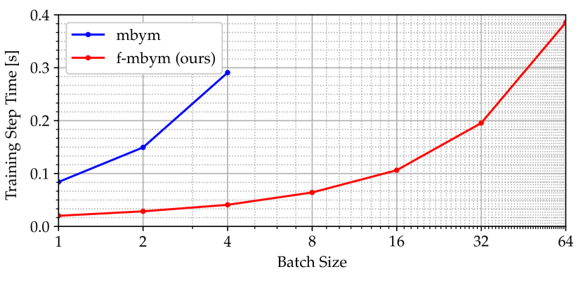
Figure 2: Training step time comparison. Note that batch size is displayed using a log scale.

V-D Masking

We now compare the performance of our approach with (f-mbym) and without (f-raw) the masking network. Comparing the odometry accuracy (Tab. III(b)) vs run-time performance (Tab. III(a)) of each method it is clear that increasing odometry accuracy is worth the added penalty to run-time performance. In the majority of cases f-mbym is still able to run in real-time whilst increasing odometry accuracy by between $345\text{\,}\mathrm{\char 37\relax}390\text{\,}\mathrm{\char 37\relax}$ across each resolution. We posit that conventional decoupled search approaches, as in [17] could experience similar boosts in performance by adopting a learnt feature representation as in our approach.

V-E Comparison To Sparse Point Based Methods

Finally, we compare our approach to several existing point-based RO systems on the Oxford Radar RobotCar Dataset [9], including: Cen RO [1], MC-RANSAC [4], HERO [5], Under The Radar [6], CFEAR [7]. For direct comparison we re-train our method using the splits from [6, 5]. As shown in Tab. IV we perform competitively with other approaches. We outperform Cen RO and MC-RANSAC by a significant margin. We also slightly outperform Under the Radar and HERO in rotational error. Only, CFEAR outperforms us in both translational and rotational error.

		Kitti Odometry Error
Method	Type	Tra ($\text{\,}\mathrm{\char 37\relax}$)	Rot ($\text{\,}\deg\mathrm{/}\mathrm{k}\mathrm{m}$)
Sparse Point-Based
Cen RO [1]	classical	3.7168	9.50
MC-RANSAC [4]	classical	3.3190	10.93
Under The Radar [6]	supervised	2.0583	6.70
HERO [5]	unsupervised	1.9879	6.52
CFEAR [7]	classical	1.7600	5.00
Dense
mbym[8]	supervised	1.1600	3.00
f-mbym (ours)	supervised	2.0597	6.269

TABLE IV: Comparison to other recent RO methods.

VI Conclusion

In contrast to the brute force search over all possible combinations of translation and angle proposed in mbym [8], we propose to decouple the search for angle and translation, exploiting the Fourier Transform’s invariance to translation. Doing so allows our approach to be trained faster and with less memory as well as to run significantly faster at inference time. By providing a greater run-time efficiency at higher resolutions our best performing real-time model achieves an end-point error of $2.01\text{\,}\mathrm{\char 37\relax}$ in translation and $6.3\text{\,}\deg\mathrm{/}\mathrm{k}\mathrm{m}$, outperforming the best real-time Masking by Moving model in accuracy whilst running $168\%$ faster on a CPU and in real-time (at $6\text{\,}\mathrm{Hz}$) on a Jetson GPU. Our approach is competitive with the current state of the art achieved by sparse, point-based methods, challenging the conventional wisdom that a sparse point-based method is necessary for real-time performance.

As per Sec. V-A the run-time performance of our approach is currently limited by the time taken to mask each radar scan using a neural network. We also note that whilst our model achieves more accurate real-time performance in comparison to [8] when considering a like-for-like comparison at each resolution a significant gap exists in odometry accuracy. Closing this gap further could allow a dense method to surpass the performance of a sparse method whilst running in real-time. Investigating whether this is achievable with the modifications to the proposed formulation alongside faster masking strategies constitute interesting areas for future research. Finally, the decoupled search developed in our approach, could also be used to efficiently search for larger rotations, and so utilised for metric localisation where the rotational offset can be arbitrary.

VII Appendix

As the affine transformation property of the Fourier Transform (FT) in  Eq. 6 is crucial to this work and the original description by Bracewell [24] is not readily available, we derive it here again for completeness, starting with the definition of the 2D FT

$$\hat{g}(\bm{\mathrm{u}}^{\prime}) =\int_{\mathbb{R}^{2}}g(\bm{\mathrm{x}}^{\prime})e^{-2\pi j{\bm{\mathrm{u}}^{\prime}}^{\top}\bm{\mathrm{x}}^{\prime}}d\bm{\mathrm{x}}^{\prime}$$ (13)

$$=\int_{\mathbb{R}^{2}}g(\bm{\mathtt{R}}^{*}\bm{\mathrm{x}}+\bm{\mathtt{t}}^{*})e^{-2\pi j{\bm{\mathrm{u}}^{\prime}}^{\top}(\bm{\mathtt{R}}^{*}\bm{\mathrm{x}}+\bm{\mathtt{t}}^{*})}d\bm{\mathrm{x}}$$ (14)

$$=e^{-2\pi j{\bm{\mathrm{u}}^{\prime}}^{\top}\bm{\mathtt{t}}^{*}}\int_{\mathbb{R}^{2}}g(\bm{\mathtt{R}}^{*}\bm{\mathrm{x}}+\bm{\mathtt{t}}^{*})e^{-2\pi j{\bm{\mathrm{u}}^{\prime}}^{\top}\bm{\mathtt{R}}^{*}\bm{\mathrm{x}}}d\bm{\mathrm{x}}$$ (15)

$$=e^{-2\pi j(\bm{\mathtt{R}}^{*}\bm{\mathrm{u}})^{\top}{\bm{\mathtt{t}}^{*}}}\int_{\mathbb{R}^{2}}f(\bm{\mathrm{x}})e^{-2\pi j\bm{\mathrm{u}}^{\top}\bm{\mathrm{x}}}d\bm{\mathrm{x}}$$ (16)

$$=e^{-2\pi j{\bm{\mathtt{t}}^{*}}^{\top}\bm{\mathtt{R}}^{*}\bm{\mathrm{u}}}\hat{f}(\bm{\mathrm{u}})$$ (17)

Eq. 14 follows from a change of variables $\bm{\mathrm{x}}^{\prime}=\bm{\mathtt{R}}^{*}\bm{\mathrm{x}}+\bm{\mathtt{t}}^{*}$ noting $d\bm{\mathrm{x}}^{\prime}=|\bm{\mathtt{R}}^{*}|d\bm{\mathrm{x}}=d\bm{\mathrm{x}}$ and Eq. 15 by expanding the exponent and from the linearity of the Fourier transform. Eq. 16 follows by defining $\bm{\mathrm{u}}^{\prime}=\bm{\mathtt{R}}^{*}\bm{\mathrm{u}}$ and substituting $f(\bm{\mathrm{x}})=g(\bm{\mathtt{R}}^{*}\bm{\mathrm{x}}+\bm{\mathtt{t}}^{*})$ as in Sec. III-A. Finally, Eq. 17 follows from the definition of the 2D Fourier transform. Substituting $\bm{\mathrm{u}}^{\prime}=\bm{\mathtt{R}}^{*}\bm{\mathrm{u}}$ and rearranging terms finally gives Eq. 6:

$$\hat{f}(\bm{\mathrm{u}}) =\hat{g}(\bm{\mathtt{R}}^{*}\bm{\mathrm{u}})e^{2\pi j{\bm{\mathtt{t}}^{*}}^{\top}\bm{\mathtt{R}}^{*}\bm{\mathrm{u}}}$$ (18)

References

- [1] S. H. Cen and P. Newman, “Precise ego-motion estimation with millimeter-wave radar under diverse and challenging conditions,” in 2018 IEEE International Conference on Robotics and Automation (ICRA), pp. 6045–6052, IEEE, 2018.
- [2] S. H. Cen and P. Newman, “Radar-only ego-motion estimation in difficult settings via graph matching,” in 2019 International Conference on Robotics and Automation (ICRA), pp. 298–304, IEEE, 2019.
- [3] R. Aldera, D. De Martini, M. Gadd, and P. Newman, “Fast radar motion estimation with a learnt focus of attention using weak supervision,” in 2019 International Conference on Robotics and Automation (ICRA), pp. 1190–1196, IEEE, 2019.
- [4] K. Burnett, A. P. Schoellig, and T. D. Barfoot, “Do we need to compensate for motion distortion and doppler effects in spinning radar navigation?,” IEEE Robotics and Automation Letters, vol. 6, no. 2, pp. 771–778, 2021.
- [5] K. Burnett, D. J. Yoon, A. P. Schoellig, and T. D. Barfoot, “Radar odometry combining probabilistic estimation and unsupervised feature learning,” in Robotics: Science and Systems, 2021.
- [6] D. Barnes and I. Posner, “Under the radar: Learning to predict robust keypoints for odometry estimation and metric localisation in radar,” in 2020 IEEE International Conference on Robotics and Automation (ICRA), pp. 9484–9490, IEEE, 2020.
- [7] D. Adolfsson, M. Magnusson, A. Alhashimi, A. J. Lilienthal, and H. Andreasson, “Cfear radarodometry-conservative filtering for efficient and accurate radar odometry,” in 2021 IEEE/RSJ International Conference on Intelligent Robots and Systems (IROS), pp. 5462–5469, IEEE, 2021.
- [8] D. Barnes, R. Weston, and I. Posner, “Masking by moving: Learning distraction-free radar odometry from pose information,” arXiv preprint arXiv:1909.03752, 2019.
- [9] D. Barnes, M. Gadd, P. Murcutt, P. Newman, and I. Posner, “The Oxford Radar RobotCar Dataset: A Radar Extension to the Oxford RobotCar Dataset,” in IEEE International Conference on Robotics and Automation (ICRA), 2020.
- [10] R. Aldera, D. De Martini, M. Gadd, and P. Newman, “What could go wrong? introspective radar odometry in challenging environments,” in 2019 IEEE Intelligent Transportation Systems Conference (ITSC), pp. 2835–2842, IEEE, 2019.
- [11] J. S. Lim, “Two-dimensional signal and image processing,” Englewood Cliffs, 1990.
- [12] D. Casasent and D. Psaltis, “Position, rotation, and scale invariant optical correlation,” Applied optics, vol. 15, no. 7, pp. 1795–1799, 1976.
- [13] X. Guo, Z. Xu, Y. Lu, and Y. Pang, “An application of fourier-mellin transform in image registration,” in The Fifth International Conference on Computer and Information Technology (CIT’05), pp. 619–623, 2005.
- [14] T. Kazik and A. H. Göktoğan, “Visual odometry based on the fourier-mellin transform for a rover using a monocular ground-facing camera,” in 2011 IEEE International Conference on Mechatronics, pp. 469–474, IEEE, 2011.
- [15] H. T. Ho and R. Goecke, “Optical flow estimation using fourier mellin transform,” in 2008 IEEE Conference on Computer Vision and Pattern Recognition, pp. 1–8, IEEE, 2008.
- [16] P. Checchin, F. Gérossier, C. Blanc, R. Chapuis, and L. Trassoudaine, “Radar scan matching slam using the fourier-mellin transform,” in Field and Service Robotics, pp. 151–161, Springer, 2010.
- [17] Y. S. Park, Y.-S. Shin, and A. Kim, “Pharao: Direct radar odometry using phase correlation,” in 2020 IEEE International Conference on Robotics and Automation (ICRA), pp. 2617–2623, IEEE, 2020.
- [18] A. V. Oppenheim, Discrete-time signal processing. Pearson Education India, 1999.
- [19] M. Jaderberg, K. Simonyan, A. Zisserman, et al., “Spatial transformer networks,” Advances in neural information processing systems, vol. 28, pp. 2017–2025, 2015.
- [20] O. Ronneberger, P. Fischer, and T. Brox, “U-net: Convolutional networks for biomedical image segmentation,” in International Conference on Medical image computing and computer-assisted intervention, pp. 234–241, Springer, 2015.
- [21] A. Odena, V. Dumoulin, and C. Olah, “Deconvolution and checkerboard artifacts,” Distill, 2016.
- [22] D. P. Kingma and J. Ba, “Adam: A method for stochastic optimization,” arXiv preprint arXiv:1412.6980, 2014.
- [23] A. Geiger, P. Lenz, and R. Urtasun, “Are we ready for autonomous driving? the kitti vision benchmark suite,” in 2012 IEEE Conference on Computer Vision and Pattern Recognition, pp. 3354–3361, IEEE, 2012.
- [24] R. Bracewell, K.-Y. Chang, A. Jha, and Y.-H. Wang, “Affine theorem for two-dimensional fourier transform,” Electronics Letters, vol. 29, no. 3, pp. 304–304, 1993.