Interpretable Molecular Graph Generation via Monotonic Constraints

Abstract

Designing molecules with specific properties is a long-lasting research problem and is central to advancing crucial domains such as drug discovery and material science. Recent advances in deep graph generative models treat molecule design as graph generation problems which provide new opportunities toward the breakthrough of this long-lasting problem. Existing models, however, have many shortcomings, including poor interpretability and controllability toward desired molecular properties. This paper focuses on new methodologies for molecule generation with interpretable and controllable deep generative models, by proposing new monotonically-regularized graph variational autoencoders. The proposed models learn to represent the molecules with latent variables and then learn the correspondence between them and molecule properties parameterized by polynomial functions. To further improve the intepretability and controllability of molecule generation towards desired properties, we derive new objectives which further enforce monotonicity of the relation between some latent variables and target molecule properties such as toxicity and clogP. Extensive experimental evaluation demonstrates the superiority of the proposed framework on accuracy, novelty, disentanglement, and control towards desired molecular properties. The code is anonymized at https://anonymous.4open.science/r/MDVAE-FD2C.

1 Introduction

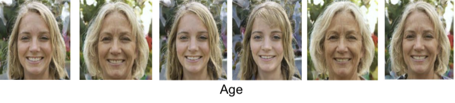
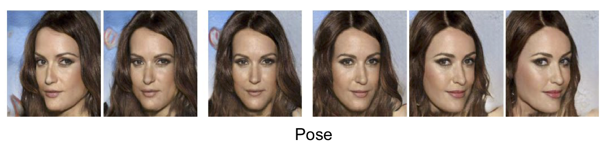
(a) Image generation without control	(b) Image generation with control
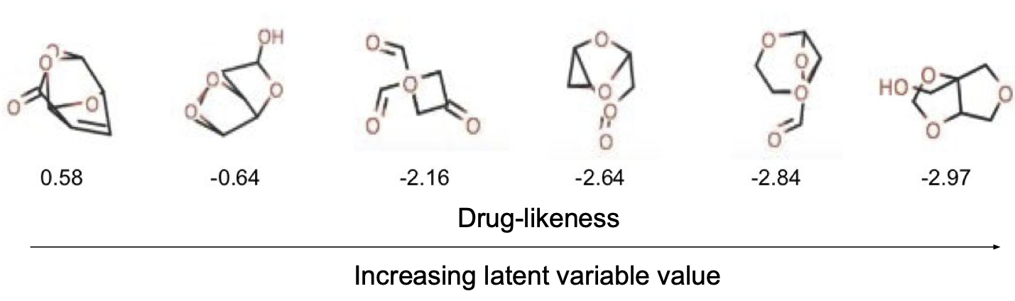
(c) Molecule generation without control	(d) Molecule generation with control

Figure 1: (a) Image generation without control: Age control is difficult, since the latent variable is not monotonically correlated with it. (b) Image generation with control: Pose control is now easy, since the latent variable is monotonically correlated with it. (c) Molecule generation without control: Drug-likeness control is difficult, since the value of latent variable is not monotonically correlated with it. (d) Molecule generation with control: Drug-likeness control is now easy, since the latent variable is monotonically correlated with it.

Designing molecules with specific structural and functional properties is central to advancing drug discovery and material science [1]. Decades of research in medicinal chemistry shows that finding novel drugs remains an outstanding challenge [2], since the search space is vast and highly rugged; small perturbations in the chemical structure may result in great changes in desired properties.

While for many years computational screening was primarily dominated by similarity search [3], recent advances in deep generative models are showing promise in tackling de-novo molecule design. The first effort addressed the problem as a string generation task by utilizing the SMILES representation [4, 5]. However, SMILES is not designed to capture molecular similarity and prevents generative models (e.g., variational auto-encoders (VAE)) from learning smooth molecular embeddings. More importantly, essential chemical properties, such as molecular weight, cannot be expressed and preserved by the SMILES representation.

Recent advances in deep generative models on graphs have opened a new research direction for de-novo molecular design. Specifically, these models leverage more expressive representations of molecules via the concept of graphs, which is a natural formulation of molecule where atoms are connected by bonds. Graph-generative models hold much promise in generating credible molecules [6, 7, 8]. The state-of-the-art deep generative models for molecule generation consist of two complementary subtasks: (1) the encoding, which refers to learning to represent molecules in a continuous manner that facilitates the preservation or optimization of their properties; (2) the decoding, which refers to learning to map an optimized continuous representation back into a reconstructed or novel molecule.

Despite promising results, the existing models have several limitations: (1) The molecule generation process is obscure. Learning the correspondence between a molecule’s structural patterns and its functional properties is one of the core issues in molecular modeling and design. However, although existing deep generative models for graphs can map the graph structural information into continuous representations, they are latent variables with no real-world meaning. Moreover, the latent variables may have mutual correlations with each other which further prevents us from understanding their meanings. Models that can characterize the correspondence between the molecule structure, latent variables, and molecule properties with better transparency are imperative and have not been well explored. (2) Difficulty in controlling the properties of the generated molecule graphs. It is important to generate molecules with desired biophysical and biochemical properties, such as toxicity, mass, and clogP [9]; However, this is a very challenging and promising domain that has not been well explored historically. The few existing works typically formulate this as a conditional graph generation problem where the targeted properties are treated as conditions. However, it is difficult to assume the distributions of the properties as most the distribution of the real-world properties are unknown or too sophisticated to be predefined. Moreover, existing works need to assume the independency among the properties which usually is also not true, for example, cLogP and cLogS are highly correlated. Thus, more powerful methods that can automatically estimate the distributions of the inter-correlated properties are imperative. Moreover, the correspondence between latent variables and properties learned by the models need to be simple (e.g., monotonic and smooth) and hence easily controllable. For example, if the correspondence is a monotonic mapping then we can enlarge the latent variable’s value to increase (or descrease) the value of a property. As shown in Fig. 1(a), tuning the age in the generated image is not easy since increasing z may or may not increase or decrease the age. Similar trouble is also in Fig. 1(c). But in Fig. 1(b) and (d), it is much easier to tune the properties thanks to the monotonic relation between latent variables and targeted properties.

In this paper, we address the above limitations by proposing a Monotonic Disentangled VAE, (MDVAE), which is a new framework that enhances the interpretability and controllability of deep graph generation of molecules. Specifically, a disentanglement loss is first introduced to enforce the disentanglement of latent variables for capturing more interpretable, factorized latent variables. In order to generate molecules with the desired properties, we then enforce a monotonic constraint over the correspondence between some latent variables and the targeted properties. Multiple strategies have also been proposed to instantiate the correspondence including linear and polynomial for the trade-off between model controllability and expressiveness. The contributions of this work are summarized as follows:

• A new framework of monotonically-constrained graph VAE is proposed for controllable generation. The proposed model encodes the molecule structure into the latent disentangled variables, which can be used to reversely generate the molecules with desired properties with potential inter-correlations.

• A polynomial parametrization for mapping latent variables to properties is introduced. Our proposed polynomial parametrization explicitly enables the model to learn the linear and non-linear relationship between the latent variables and the desired properties with better trade-off between model capacity and transparency.

• Various monotonic constraint strategies are proposed for regularizing the mapping between latent variables and molecule properties toward better controllability. Gradient-based and direction-based monotonic constraints are both proposed to regularize the mapping between latent variables and molecule properties. Such constraints have further been generalized to handle the situation when molecule properties are correlated.

• Extensive experiments demonstrated the effectiveness, interpretability, and controllability of our proposed models. Qualitative and quantitative evaluations on multiple benchmark datasets demonstrated that the proposed models have outperformed the state-of-the-art methods by generating more accurate and better molecules by up to 68% improvement in learning a more accurate molecular property distribution, up to 43% improvement in interpretability, and up to 34% improvement in controlling the molecular properties.

2 Related Work

Early deep learning-based works in [4, 10, 11] built generative models of SMILES strings with recurrent decoders. SMILES is a formal grammar that describes molecules with an alphabet of characters. For instance, ‘c’ and ‘C’ denote aromatic and aliphatic carbon atoms; ‘O’ denotes the oxygen atom; ‘-’ denotes single bonds; ‘=’ denotes double bonds, and so on. Since initial models could generate invalid molecules, later works [5, 12] introduced syntactic and semantic constraints by context-free and attribute grammars; yet, the resulting models could not fully capture chemical validity. Other methods aimed to generate valid molecules by leveraging active learning [13] and reinforcement learning [14].

Graph-generative models now present an alternative approach to molecule generation. For example, work in [6] generates molecular graphs by predicting their adjacency matrices. Work in [15] generates molecules through a constrained graph generative model that enforces validity by generating the molecule atom by atom. The majority of existing models are based on the VAE framework [6, 16, 17, 18, 19, 20, 21, dudeeplatent2021, 22] or generative adversarial networks (GANs) [23, 24, 25], and others [26, 15, 27, 28, 29, 30]. For instance, GraphRNN [26] builds an autoregressive generative model based on a generative recurrent neural network (RNN) by representing the graph as a sequence and generating nodes one by one. In contrast, GraphVAE [6] represents each graph in terms of its adjacent matrix and feature vectors of nodes. A VAE model is then utilized to learn the distribution of the graphs conditioned on a latent representation at the graph level. Other works [31, 32] encode the nodes of each graph into node-level embeddings and predict the links between each pair of nodes to generate a graph.

In this work, we leverage recent advances in disentangled representation learning to further advance molecule generation.

Currently, disentangled representation learning based on VAE is mainly limited in the domain of image representation learning [33, 34, 35, 36]. The goal is to learn representations that separate out the underlying explanatory factors responsible for formalizing the data. Disentangled representations are inherently more interpretable and can, thus, potentially facilitate debugging and auditing [33, 34, 37, 36, 38, 39].

However, how to best learn representations that disentangle the latent factors behind a graph remains largely unexplored. Though few works are proposed for interpreting the graph representations [40], they do not focus on the graph generation task. In addition, utilizing disentanglement learning for molecule generation with desired properties is critical yet seldom explored.

3 Methods

Figure 2: (a) The conditional models of the baseline models and our proposed models, including the encoder (left) and the decoder (right). The encoder encodes a molecular graph to a smooth latent representation. The decoder decodes a novel molecular graph from the latent representation (and a property Y). Dotted node represents disentangled latent representation, dotted line denotes polynomial and monotonic constraints. (b) MDVAE Framework. Molecule is represented as a graph, atom as a node, bond as a edge. The encoder encodes the graph into latent representation $z$, characterized by mean $z_{\mu}$ and $z_{\sigma}$, where disentalgment is enhanced. The decoder decodes the novel molecule from the latent representation. (c) Monotonic constraint is enforced in the latent representation $z$ to control the relationship between the latent variables and the observed properties.

3.1 Problem Formulation

The structure of a molecule can be defined as a graph $G=(\mathcal{V},\mathcal{E},E,F)$, where $\mathcal{V}$ is the set of $N$ nodes (the atoms) and $\mathcal{E}\subseteq\mathcal{V}\times\mathcal{V}$ is the set of $M$ edges (the bonds that connect pairs of atoms). $e_{i,j}\in\mathcal{E}$ is an edge connecting nodes $v_{i}\in\mathcal{V}$ and $v_{j}\in\mathcal{V}$. $E\in\mathbb{R}^{N\times N\times K}$ refers to the edge type tensor (i.e. bond type), where $E_{i,j}\in\mathbb{R}^{1\times K}$ is an one-hot vector encoding the type of edge $e_{i,j}$. $K$ is the number of edge types. $F\in\mathbb{R}^{N\times K^{\prime}}$ refers to a node’s feature matrix, where $F_{i}\in\mathbb{R}^{1\times K^{\prime}}$ is the one-hot encoding vector denoting the type of atom $v_{i}\in\mathcal{V}$, and $K^{\prime}$ is the total number of atom types. We also pre-define a set of molecular properties, such as clogP and molecular weight, as a vector of real-valued variables $Y=\{Y^{(1)},\ldots,Y^{(J)}\}$, where $Y^{(j)}$ is the value of the $j$-th property.

Our goal is to learn the generative process $p(G,Y|Z)$ of a molecule $G$ and its properties $Y$, characterized by latent variables $Z$. Considering that this process is obscure to be fully prescribed, we aim at characterizing it in a data-driven manner by latent variables $Z$ learned automatically by end-to-end deep generative models (e.g., VAEs and GANs). To further enhance the interpretability and controllability of $Z$, we will also aim to disentangle the latent variables and maximize the correspondence between (some of) them and the real molecule properties.

3.2 Monotonically Disentangled VAE (MDVAE)

Here we first introduce the proposed MDVAE model and its inference. Then we describe how to further enforce disentanglement among latent variables as well as their monotonic relation to molecule properties.

3.2.1 Disentangled Deep Generative Models for Molecule Graphs.

Learning $p_{\theta}(G,Y|Z)$ requires the inference of its posterior $p_{\theta}(Z|G,Y)$. Because this inference is intractable, we need to define an approximated posterior $q_{\phi}(Z|G,Y)$ that is computationally tractable. We then minimize the Kullback–Leibler divergence (KLD) between them $D_{KL}(q_{\phi}(Z|G,Y)\|p_{\theta}(Z|G,Y))$ to ensure that the approximated posterior is close to the true posterior. This is well-known to amount to maximizing the evidence lower-bound ([41]), as follows:

(3.1) $$\max_{\theta,\phi} \mathbb{E}_{q_{\phi}(Z|G,Y)}[\log p_{\theta}(G,Y|Z)]$$

$$-\lambda\sum\nolimits_{i}^{N}D_{\operatorname{KL}}(q_{\phi}(Z_{i}|G,Y)\|p(Z_{i}))$$

where $\phi$ is the parameter of the approximated posterior $q_{\phi}$. The prior $p(Z)$ follows an isotropic Gaussian such that each $Z_{i}$ is independent of the others. Hence, the KL Divergence in the second term between $q_{\phi}(Z|G,Y)$ and $p(Z)$ will encourage the disentanglement among the variables in $Z$ in the inferred $q_{\phi}(Z|G,Y)$. Here $\lambda$ can control the strength of this enforcement, and the lager it is, the more independence different variables in $Z$ will have. This can be achieved if we set the prior to be an isotropic unit Gaussian, i.e. $p(Z)=\mathcal{N}(\mathbf{0},I)$, leading to the constrained optimization problem $\max_{\theta,\phi}\mathbb{E}_{G\thicksim\mathcal{D}}[\mathbb{E}_{q_{\phi}(Z|G,Y)}logp_{\theta}(G,Y|Z)]$ under the condition that $D_{KL}(q_{\phi}(Z|G,Y)||p(Z))\leq\epsilon$, where $\epsilon$ specifies the strength of the applied constraint; $\mathcal{D}$ refers to the observed set of molecules, and $D_{KL}(\cdot)$ denotes the Kullback–Leibler divergence (KLD) between two distributions. Considering $Z$ is conditionally independent to $Y$ given $G$ yields $q_{\phi}(Z|G,Y)=q_{\phi}(Z|G)$ and DIP-VAE [42] introduces disentanglement enforcement term $D(q_{\phi}(Z)||p(Z))$ with loss:

(3.2) $$\max_{\theta,\phi}\mathbb{E}_{q_{\phi}(Z|G)}[\mathrm{log}p_{\theta}(G|Z)]-\alpha D(q_{\phi}(Z)||p(Z))$$

$$+\mathbb{E}_{q_{\phi}(Z|G)} [\mathrm{log}p_{\theta}(Y|G,Z)]-\lambda\sum\nolimits_{i}^{N}D_{KL}(q_{\phi}(Z_{i}|G)||p(Z_{i}))$$

which enforces the monotonicity of the relation between $Z$ and $Y$ in the following:

3.2.2 Monotonic Correlation towards Targeted Properties

Disentanglement among latent variables $Z$ is deemed to improve the interpretability of VAE models ([43]). Here we go beyond this to correlate a subset of latent variables to important molecular properties (e.g., drug-likeness, water solubility, and clogP) to further enhance the interpretability of our latent variable, as well as better control the generated molecule’s properties via tuning of the latent variables.

Specifically, we have two aims: (1) Aim 1: Correlating latent variables and real properties: We explicitly relate one of the latent variables $Z_{j}\in Z$ in the disentangled latent representation to the predefined property set $Y_{j}$ in a pairwise style; (2) Aim 2: Enforcing monotonic correlation: We accommodate the non-linearity of the correlation between latent variables and targeted properties but encourage monotonic correlation, in order to ensure that the correlation is either positive or negative for effective control. This means that if we want to increase (or decrease) a given property, we can just increase (or decrease) the corresponding latent variable’s value accordingly.

For the first aim, we first consider the scenario where the molecule properties are independent with each other:

(3.3) $$\max_{\theta,\phi}\mathbb{E}_{q_{\phi}(Z|G)}[\mathrm{log}p_{\theta}(G|Z)]-\alpha D(q_{\phi}(Z)||p(Z))$$

$$+\sum\nolimits_{j}^{J}\mathbb{E}_{q_{\phi}(Z|G)}[\mathrm{log}p_{\theta}(Y_{j}|Z_{j})]$$

$$-\lambda\sum\nolimits_{i}^{N}D_{KL}(q_{\phi}(Z_{i}|G)||p(Z_{i}))$$

where each property $Y_{j}$ corresponds to each latent variable $Z_{j}$, meaning $p(Y_{j}|Z)=p(Y_{j}|Z_{j})$. This also leads to conditional independence between $G$ and $Y_{j}$ given $Z_{j}$, meaning $p_{\theta}(Y_{j}|G,Z_{j})=p_{\theta}(Y_{j}|Z_{j})$.

For the second aim, to enforce the monotonic relationship between properties and latent variables, we require for any property $j$ that we have $\forall Z_{j}^{(1)}\leq Z_{j}^{(2)}:Y_{j}^{(1)}\leq Y_{j}^{(2)}$, where $Z_{j}^{(1)},\ Z_{j}^{(2)}$ are two values of latent variable $Z_{j}$ from $q_{\phi}(Z_{j}|G)$, while $Y_{j}$ refers to any molecule property. The overall objective of our model is now reformulated as:

(3.4) $$\max_{\theta,\phi}\mathbb{E}_{q_{\phi}(Z|G)}[\mathrm{log}p_{\theta}(G|Z)]-\alpha D(q_{\phi}(Z)||p(Z))$$

$$+\sum\nolimits_{j}^{J}\mathbb{E}_{q_{\phi}(Z|G)}[\mathrm{log}p_{\theta}(Y_{j}|Z_{j})$$

$$-\lambda\sum_{i}D_{KL}(q_{\phi}(Z_{i}|G)||p(Z_{i}))$$

$$s.t.\forall Z_{j}^{(1)} \leq Z_{j}^{(2)}:Y_{j}^{(1)}\leq Y_{j}^{(2)},Z_{j}^{(1)},Z_{j}^{(2)}\sim q_{\phi}(Z_{j}|G).$$

As mentioned above, $Y_{j}$ is dependent merely on $Z_{j}$, so we can define a function mapping $F_{j}:\mathbb{R}\rightarrow\mathbb{R}$ from $Z_{j}$ to $Y_{j}$. $F_{j}$ can be any function such as polynomial or multi-layer perceptron that can effectively fit arbitrarily complex (non-)linear mapping. Enforcing the constraint of Equation (3.4) is equivalent to enforcing the monotonicity of function $F_{j}$.

3.3 Monotonic Regularization of MDVAE

As mentioned in the discussion under Equation (3.4), we need to enforce the monotonicity of $F_{j},\ j=\{1,\cdots,J\}$. This amounts to penalizing the violation of constraints via an additional regularization term $\mathcal{R}$ together with the original objective in Equation (3.4). In the following, we propose two different ways.

Gradient-based monotonic regularization. In this way, we enforce that the gradient of function $F_{j}(Z_{j})$ is always positive or negative to enforce its monotonicity. Without loss of generality, here we require the derivative to be always positive. That means we want to enforce that $\frac{\mathrm{d}F_{j}(Z_{j})}{\mathrm{d}Z_{j}}\geq 0$, where $Z_{j}$ is any of the latent variables. Hence, the following regularization term will punish its violation: $\max(0,-\frac{\mathrm{d}F_{j}(Z_{j})}{\mathrm{d}Z_{j}})$.

This term can be implemented using the following regularization term $\mathcal{R}(Z)$ using ReLU [44], as in:

(3.5) $$\mathcal{R}(Z)=\sum\nolimits_{j}^{J}\mathbb{E}_{q_{\phi}(Z|G)}\mathrm{ReLU}[-\frac{\mathrm{d}F_{j}(Z_{j})}{\mathrm{d}Z_{j}}]$$

where $J$ refers to the number of the targeted molecule properties. Note that without loss of generality, we only consider $Z_{j}$ as a scalar here. However, our framework can be easily extended to handle multiple latent variables by generalizing it as a vector; for each element in this vector, one can perform a ReLU operation the same as that in Eq. 3.5 and then sum up all of those corresponding to the multiple variables involved.

Direction-based monotonic regularization. The second way starts from the standard definition of monotonicity: $(F_{j}(x_{1})-F_{j}(x_{2}))\cdot(x_{1}-x_{2})\geq 0$, where $x_{1},\ x_{2}$ are any latent variables. Such nonlinear constraint is difficult to enforce, so we instead penalize the following term in the objective as an equivalence: $\max(0,-(F_{j}(x_{1})-F_{j}(x_{2}))\cdot(x_{1}-x_{2}))$, which can be implemented using the following regularization term $\mathcal{R}(y,Z)$ via ReLU function as well as additional denotations:

$$\mathcal{R}(Y,Z)= \sum\nolimits_{j}^{J}\mathbb{E}_{G_{1},G_{2}\sim p_{\theta}(G|Z)}$$

(3.6) $$[\sum\nolimits_{i}^{N}\mathrm{ReLU}[-(Y_{j}^{G_{1}}-Y_{j}^{G_{2}})(Z_{j}^{G_{1}}-Z_{j}^{G_{2}})],$$

where $J$ refers to the number of the molecule properties, and $Y_{j}^{G_{k}}$ refers to the $j$-th molecule property of the molecule $G_{k}$. The molecule $G_{1}$ and $G_{2}$ are two arbitrary molecules sampled from the distribution of the observed graphs, and $Z_{j}^{G_{1}}$, $Z_{j}^{G_{2}}$ are $j$-th latent variable of them. Note that without loss of generality, our denotation here only considers $Z_{j}^{G_{k}}$ as a scalar, but our framework can be easily extended to handle multiple latent variables by generalizing it as a vector, similar to the Gradient-based approach.

Table 1: Novelty, uniqueness, and validity are measured on molecule datasets generated by the various models under comparison. The highest value on a metric is highlighted in bold font.

Dataset Metric ChemVAE GrammarVAE GraphVAE GraphGMG LSTM CGVAE DVAE MDVAE QM9 % Validity 10.00 30.00 61.00 - 94.78 100.00 100.00 100.00 % Novelty 90.00 95.44 85.00 - 82.98 96.33 98.10 98.23 % Unique 67.50 9.30 40.90 - 96.94 98.03 99.10 99.46 ZINC % Validity 17.00 31.00 14.00 89.20 96.80 100.00 100.00 100.00 % Novelty 98.00 100.00 100.00 89.10 100.00 100.00 100.00 100.00 % Unique 30.98 10.76 31.60 99.41 99.97 99.82 99.84 99.98

Generalization of group-based correlated properties. To handle the situations when some molecule properties are correlated, we generalize the above framework to the group-based disentanglement strategy.

We define $j$-th group of variables $\mathcal{Z}_{j}\subseteq Z$ which correlate to a group of molecule properties $\mathcal{Y}_{j}\subseteq Y$. Hence, the overall learning objective for the group-based disentanglement learning (Eq. (3.4) + Eq. (3.5)) is:

(3.7) $$\max_{\theta,\phi}\mathbb{E}_{q_{\phi}(Z|G)}[\mathrm{log}p_{\theta}(G|Z)]-\alpha D(q_{\phi}(Z)||p(Z))$$

$$-\lambda\sum\nolimits_{i}^{N}D_{KL}(q_{\phi}(Z_{i}|G)||p(Z_{i}))$$

$$+\beta\sum\nolimits_{j}\sum\nolimits_{i}\mathbb{E}_{q_{\phi}(Z|G)}[\log p_{\theta}(\mathcal{Y}_{j,i}|\mathcal{Z}_{j})$$

$$-\gamma\sum\nolimits_{j}\sum\nolimits_{i}\mathbb{E}_{q_{\phi}(Z|G)}\mathrm{ReLU}[-\frac{\partial F_{j}(\mathcal{Z}_{j})}{\partial\mathcal{Z}_{j,i}}],$$

4 Results

This section reports on qualitative and quantitative experiments carried out to evaluate the performance of the proposed MDVAE model. All experiments are conducted on a 64-bit machine with an NVIDIA GPU (GeForce RTX 2080Ti, 1545MHz, 11GB GDDR6).

Experiment Set-up

We compare MDVAE with $6$ state-of-the-art deep generative models on molecules: CGVAE [45], GraphGMG [46], SMILES-LSTM [47], ChemVAE [4], GrammarVAE [5], GraphVAE [6], detailed in Supplementary Material. We use the gradient-based approach for MDVAE during the experiments. Further, we add to this list the Disentangled VAE (DVAE) to serve as a baseline model. DVAE shares a similar objective with MDVAE but utilizes a linear reparametrization function rather than MDVAE’s monotonic regularization term and polynomial reparametrization. It is worth noting that CGVAE [45] has a similar encoder and decoder to the proposed MDVAE and DVAE models but does not contain the proposed disentanglement and monotonic enforcement. So, the comparison of MDVAE with CGVAE represents an ablation study that allows us to test the effectiveness of the proposed disentanglement and monotonic enforcement in MDVAE and the comparison of MDVAE with DVAE represent an ablation study that test the effectiveness of polynomial reparametrization and monotonic enforcement. Detailed model hyperparameters and architectures can be found in Supplementary Material.

Datasets

We consider two popular benchmark datasets. (1) The QM9 Dataset [48] consists of around 134k stable small organic molecules with up to $9$ heavy atoms (Carbon (C), Oxygen (O), Nitrogen (N) and Fluorine (F)), with a 120k/20k split for training versus validation. (2) The ZINC Dataset [49] contains around 250k drug-like chemical compounds with an average of around $23$ heavy atoms, with a 60k/10k split for training versus validation.

4.1 Comparison with State-of-the-art Methods

We first evaluate and compare the quality of generated molecules across the various deep generative models. All models are trained on each of the two benchmark datasets, and $30,000$ molecules are then generated/sampled from each trained model for the purpose of evaluation.

Table 1 reports on three popular metrics: novelty, which measures the fraction of generated molecules that are not in the training dataset; uniqueness, which measures the fraction of generated molecules after and before removing duplicates; and validity, which measures the fraction of generated molecules that are chemically valid. As Table 1 shows, CGVAE, MDVAE, and DVAE achieve $100\%$ validity; that is, $100$% of generated molecules are chemically-valid, which is significantly higher than other methods. This is due to the sequence decoding process, which takes a valency check step by step and so ensures that generated molecules are valid.

Table 1 also shows that MDVAE and DVAE generate up to $100\%$ novel molecules, which is higher than other methods, including CGVAE. Note that CGVAE shares a similar architecture with MDVAE and DVAE but without the disentanglement enforcement. This allows us to conclude that the higher novelty achieved by MDVAE and DVAE is due to the disentangled representation, which can fully explore molecular patterns. In particular, adding the disentanglement regularization does not affect the reconstruction error and so does not sacrifice the quality of generated molecules. We note that the LSTM method also works well on the ZINC dataset but worse on the QM9 dataset, which has a more complex data distribution with drug-like molecules. Our models and CGVAE have the highest performance on uniqueness, over $99$%.

Table 2: Evaluation of disentanglement on the QM9 and ZINC datasets.

Dataset Model $\beta$-M (%)$\uparrow$ F-M(%)$\uparrow$ DCI$\uparrow$ Mod$\uparrow$ QM9 CGVAE 100 72.0 0.151 0.634 DVAE 100 76.4 0.152 0.671 MDVAE 100 78.8 0.209 0.690 ZINC CGVAE 100 61.6 0.109 0.604 DVAE 100 62.4 0.111 0.611 MDVAE 100 64.4 0.156 0.621

Figure 3: MI heatmaps between latent variables and molecular properties (cLogP, cLogS, molecular weight, and drug-likeness. MI is normalized between 0 and 1) (better seen in color).

4.2 Evaluating Impact of Disentanglement

We now further compare CGVAE, DVAE, and MDVAE in Table 2 on disentanglement of the learned latent distributions. We utilize four popular metrics to do so: $\beta$-M[35], F-M[36], MOD [50], DCI [51], detailed explanations can be found in Supplementary Material.

Table 2 shows that our models achieve the best overall disentanglement scores. Specifically, all models achieve $100$ on the $\beta$-M score on both datasets. On the F-M score, on both datasets, MDVAE performs best, followed by DVAE, and CGVAE in this order. Similar ranking is observed on the DCI and Mod scores on both datasets. On the DCI score, DVAE performs slightly higher than CGVAE, with MDVAE performing much better than both. Similar observations hold on the Mod score comparison. It is worth noting that all three models are challenged more by the ZINC than the QM9 dataset with regards to the DCI score; the ZINC dataset is larger and contains larger molecules, as well, and it is possible that this results in more latent variables. Altogether, these results show that the proposed MDVAE and DVAE can successfully learn the disentangled latent representations better than CGVAE.

4.3 Performance in Molecular Property Control

Here, CGVAE, DVAE, and MDVAE are evaluated on whether the latent variables capture desired properties. First, we identify four properties, cLogP, cLogS, molecular weight, and drug-likeness to evaluate further (the linear correlation of paired molecular properties is visualized in Supplementary Material; specifically, we utilize mutual information (MI), implemented via the the scikit-learn library, to measure the mutual dependency between each latent variable and each of the four above properties. These results are related via heatmaps in Figure 3, which shows the MI for the pairs ($z_{0}$, clogP), ($z_{1}$, cLogS), ($z_{2}$, molecular weight), and ($z_{3}$, drug-likeness). To make CGVAE comparable to our polynomial reparameterization and monotonic constraint, we implement a linear control over the latent representation $z$ and properties $p$. It is clear that the polynomial function greatly increases property control; a much larger MI is achieved with all four properties. DVAE ranks second, which shows that disentanglement enhancement improves controllability. The other latent variables do not interfere with the properties with which we pair the specific latent variables $z_{0}-z_{4}$. The conditioning on drug-likeness has a strong control over the cLogP property; even though we do not observe a linear correlation between these two properties, drug discovery literature shows that drug-likeness is correlated to cLogP [9].

4.4 Qualitative Evaluation for Disentanglement and Property Control

We demonstrate qualitatively that MDVAE and DVAE consistently discover latent variables and use them to control molecular properties in a monotonous fashion. By jointly changing the value of one latent variable continuously and fixing the remaining latent variables, we can visualize the corresponding variation of molecular properties in the generated graphs. Figure 4 plots the variation of each property along with the change of its target latent variable. More results can be found in Supplementary Material.

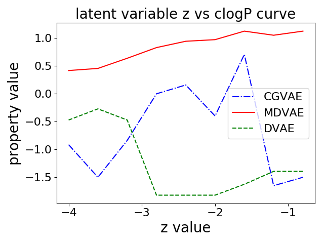
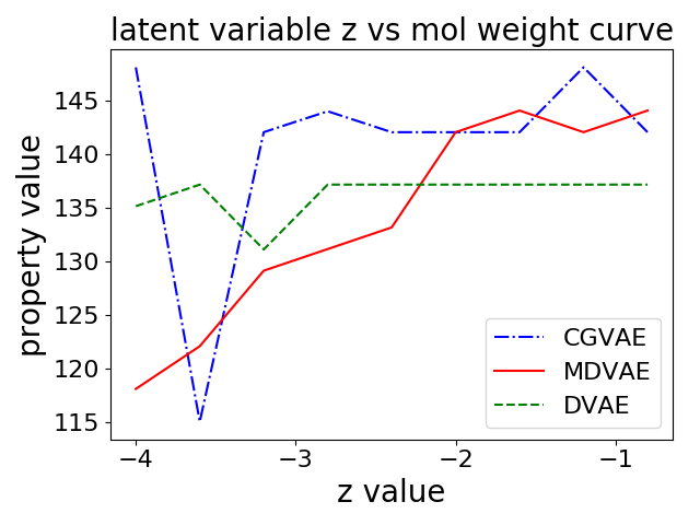
Figure 4: The relationship between the latent variable $z_{i}$ and properties of the molecules generated by CGVAE, DVAE, and MDVAE.

Figure 4 shows that MDVAE monotonically captures the disentangled latent variables that control molecular weight and drug-likeness. There are obvious fluctuations of all four properties when controlled by the latent variables learned from DVAE and CGVAE (see the green and blue lines). This is most visible in the steep decrease and increase of clogS when $z$ ranges from $-4$ to $-1$, while the property of the generated molecules by MDVAE monotonically decreases (see the red solid line). This demonstrates that the proposed monotonic correlation regularization term is necessary and effective in preserving the monotonic correlation between each molecule property and its relevant latent variable for better control of the molecule generation to obtain the desired properties.

Finally, in Figure 5 we show how generated molecules change when the value of the latent variable $z_{0}$ and $z_{1}$ changes from $-5$ to $5$ and $5$ to $-5$. The molecular weight scores are shown at the bottom of each molecule. Compared to DVAE, the proposed MDVAE model is more powerful at generating valid and high-quality molecules along with the variation of the latent variables. We can observe that molecular weight increases with the increase of the value of one of the latent variables. More results can be found in Supplementary Material.

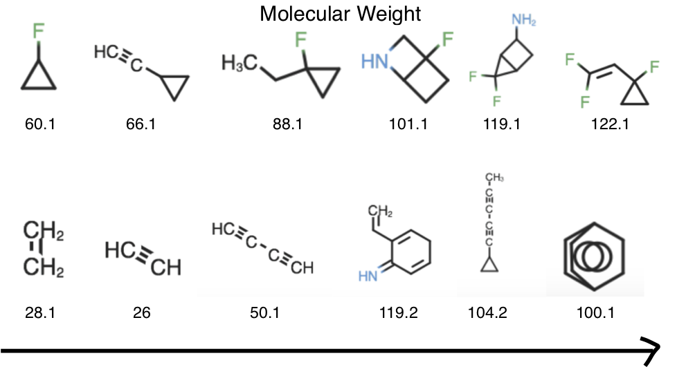
Figure 5: Molecules generated by MDVAE (top row) and DVAE (bottom row) as we increase the value of the latent variable for molecular weight.

5 Conclusion

This paper proposes a new disentangled deep generative framework for interpretable molecule generation with property control via a graph-based disentangled VAE. We derive new objectives which further enforce non-linearity and monotonicity of the relation between some latent variables and target molecule properties. The proposed models are validated on two real-world molecule datasets for three tasks: molecule generation, disentangled representation learning, and control of the generation process. Quantitative and qualitative evaluation results show the promise of disentangled representation learning in interpreting and controlling molecular properties during the generation process.

A Supplemental Material

A.1 Comparison Methods

MDVAE is compared to $6$ state-of-the-art deep generative frameworks: (1) CGVAE [45], a VAE-based model consisting of a graph-structured encoder and decoder; (2) GraphGMG [46], a deep auto-regressive graph model that generates graph nodes sequentially; (3) SMILES-LSTM [47], an LSTM model that utilizes the SMILES representation; (4) ChemVAE [4], a generative model that converts discrete representations of molecules to and from a multidimensional continuous representation; (5) GrammarVAE [5], a VAE-based model that enforces syntactic and semantic constraints over SMILES strings via context free and attribute grammars; and (6) GraphVAE [6], a generic deep generative model for graph generation.

A.2 Metrics to Measure Disentanglement

$\beta$-M[35] measures disentanglement by examining the accuracy of a linear classifier that predicts the index of a fixed factor of variation. F-M[36] addresses several issues by using a majority voting classifier on a different feature vector that represents a corner case in the $\beta$-M. MOD [50] measures whether each latent variable depends on at most a factor describing the maximum variation using their mutual information. DCI [51] computes the entropy of the distribution obtained by normalizing the importance of each dimension of the learned representation for predicting the value of a factor of variation. All implementation details are in the work proposed by [52].

Table 3: Encoders and decoders architectures of MDVAE for QM9 and ZINC dataset (Each layers is expressed in the format as $<kernel\_size><layer\_type><Num\_channel><Activation\_function><stride\_size>$. FC refers to the fully connected layers).

Encoder Decoder Input: $G(\mathcal{V},\mathcal{E},E,F)$ Input$[z]\in\mathbb{R}^{100}$ FC.100 ReLU FC.100 ReLU GGNN.100 ReLU GGNN.100 ReLU GGNN.100 ReLU GGNN.100 ReLU FC.100 FC.bv (batch node size) FC.3 (edge)

Table 4: hyper-paramter used for training on dSprites and QM9 datasets

Dataset Learning_rate Batch_size $\lambda$ Num_iteration QM9 5e-4 64 1 10 ZINC 5e-4 8 1 5

A.3 Model Complexity Analysis

The proposed DVAE and MDVAE models share the same time complexity with the baseline CGVAE model, which is based on a typical Gated Graph Neural Network (GNN) to encoder the molecules and is of linear growth with respect to the number of node $N$, and the decoder part is formulated as a sequential generation process, where the worst case time complexity is $O(N^{2})$. Overall, our models amount to a worst case $O(N^{2})$ time complexity, which is scalable compared to the state-of-the-art graph generative models, worst case $O(N^{4})$ for graphVAE [6] and worst case $O(N^{2})$ for graphRNN [26].

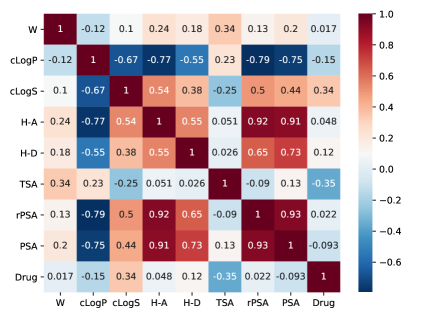
Figure 6: Heatmap showing the linear correlation between each pair of the given properties. Each entry is the correlation score between a pair of properties of molecule.

A.4 Implementation of MDVAE

The construction of the overall model extends the conventional VAE consisting of an encoder and a decoder, where the former implements the inference model $q_{\phi}(Z|G)$ while the latter instantiates the generator $p_{\theta}(G|Z,Y)$.

Molecule Encoder To model the prior distributions $q_{\phi}(Z|G)$ expressed in the objective, an encoder is constructed based on a graph neural network (GNN). The GNN embeds each node in an input graph $G$ into $L$-dimension latent space following distribution $q_{\phi}(Z|G)$ parameterized by mean $\mu_{i}$ and standard deviation vectors $\sigma_{i}$ for each node $v_{i}$, which is the output of the GNN. Note the model handles the inputs of different sizes by setting a maximum number of vertices and mask on the padded nodes in each batch. To compensate the changing maximum vertices for each batch, the model is designed to pass into the network by the hidden size (h) rather than number of vertices $\times$ the hidden size ($v\times h$) as other regular GNN does. In the end, by sampling from the modeled distribution, $Z=\{Z_{1},...,Z_{N}\}$ are obtained variables containing the node representation vectors for all the nodes.

Molecule Decoder The molecule decoder models the distribution $p_{\theta}(G|Z)$ by generating the molecule graph $G$ conditioning on the latent representation variables $Z$ that are sampled from the learned distribution in the encoder. The process proceeds in an auto-regressive style. In each step a focus node is chosen to be visited, and then the edges are generated related to this focus node are generated. The nodes are ordered by using the breadth-first traversal. The molecule decoder mainly contains three steps, namely node initialization, node update and edge selection and labeling. The detailed implementation of the encoder and decoder is based on the work by [15].

A.5 Hyperparameter Details

Table 5: Encoders and decoders architectures of MDVAE for QM9 and ZINC dataset (Each layers is expressed in the format as $<kernel\_size><layer\_type><Num\_channel><Activation\_function><stride\_size>$. FC refers to the fully connected layers).

Encoder Decoder Input: $G(\mathcal{V},\mathcal{E},E,F)$ Input$[z]\in\mathbb{R}^{100}$ FC.100 ReLU FC.100 ReLU GGNN.100 ReLU GGNN.100 ReLU GGNN.100 ReLU GGNN.100 ReLU FC.100 FC.bv (batch node size) FC.3 (edge)

Table 6: hyper-paramter used for training on dSprites and QM9 datasets

Dataset Learning_rate Batch_size $\lambda$ Num_iteration QM9 5e-4 64 1 10 ZINC 5e-4 8 1 5

A.6 Comparison of the Learned to the Reference Distribution

The above analysis indicates that CGVAE, DVAE, and MDVAE are the top three models, so we now focus on further evaluation of these three models. In particular, we now compare the reference/training dataset to the dataset generated by a model. Each dataset is summarized via a distribution of a variable of interest. The divergence between two distributions is measured via popular metrics, such as the Maximum Mean Discrepancy (MMD) [26] and the Kullback-Leibler Divergence (KLD) [26].

Table 7: Comparison of training and generated distributions of graph properties via MMD and KLD. (CC refers to the Clustering Coefficient).

Dataset Metric CGVAE DVAE MDVAE QM9 MMD(Degree) 0.0985 0.1133 0.0456 MMD (CC) 0.0215 0.0242 0.0192 MMD (Orbit) 0.0179 0.0130 0.0057 KLD (cLogP) 0.3102 0.2744 0.1935 KLD (cLogS) 0.2886 0.2297 0.1358 KLD (Drug-like) 0.0100 0.1261 0.0099 KLD (PSA) 0.3921 0.2931 0.2277 KLD (Mol Weight) 3.1360 1.7641 1.7005 ZINC MMD (Degree) 0.0050 0.0057 0.0045 MMD (CC)) 0.0012 0.0008 0.0004 MMD (Orbit) 0.0011 0.0018 0.0011 KLD (cLogP) 0.1888 0.0503 0.0428 KLD (cLogS) 0.0641 0.0494 0.0483 KLD (Drug-like) 1.4590 0.7671 0.3268 KLD (PSA) 0.1918 0.3159 0.1686 KLD (Mol Weight) 0.1191 0.1296 0.1115

We utilize three popular graph-summarization variables [26, 15]: node degree, clustering coefficient, and average orbit count; the latter counts the number of $4$-orbits in a graph. Distributions are compared via MMD. In addition, we utilize benchmark molecular properties utilized in medicinal chemistry to evaluate molecular compounds, such as cLogP, cLogS, Drug-likeness, Polar Surface Area (PSA), and Molecular Weight [45] and use KLD to compare resulting distributions. Briefly, cLogP measures hydrophilicity and evaluates the absorption or permeation of a compound; cLogS provides complementary information on aquous solubility; Drug-likeness is partially based on topological descriptors; PSA evaluates the cell permeability of a compound; and molecular weight provides information on both compound activity and permeability.

Table 7 shows that on the QM9 dataset, the MDVAE-generated dataset is more similar to the reference dataset than the DVAE- and CGVAE-generated datasets; the smaller the value is, the more similar the generated properties are to those in the training set. Similarly, all MMD values are reasonably small, suggesting that DVAE and MDVAE also preserve graph patterns of the reference distribution. All three models perform poorly on the molecular weight property, especially on the QM9 drug-like molecule dataset. We suspect the reason is that the drug-like molecule distribution is harder to learn. Comparably, all three models preserve the reference distribution more on the ZINC than on the QM9 dataset.

Figure 9 provides some more detail and relates the distribution of generated molecules superimposed over the distribution of the reference dataset (in terms of selected molecular properties). Figure 9 shows that there is good agreement between the generated and reference distributions. Of all the three models, MDVAE performs best, yielding greatest overlap between the generated data property distribution and the reference dataset property distribution. Nevertheless, DVAE and CGVAE perform comparably well, with DVAE slightly outperforming CGVAE.

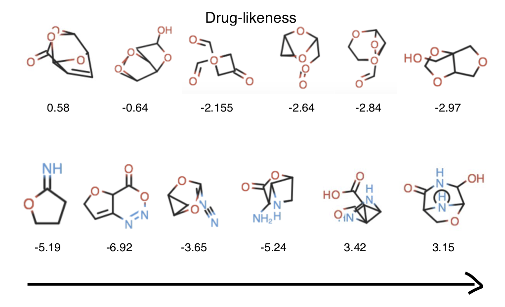
Figure 7: Molecules generated by MDVAE (top row) and DVAE (bottom row) as we increase the value of the latent variable by enforcing the molecular weight (left) and drug-likeness (right).

CGVAE
clogP	clogS
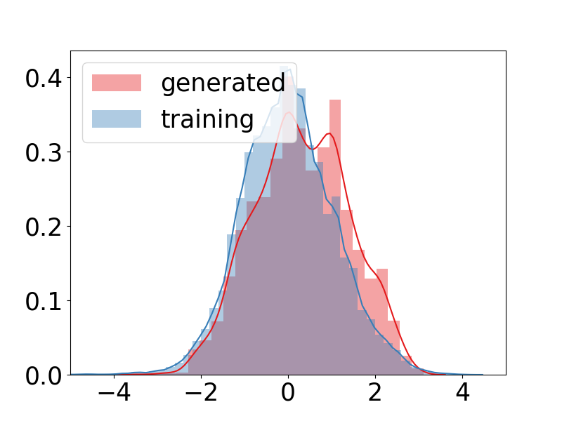
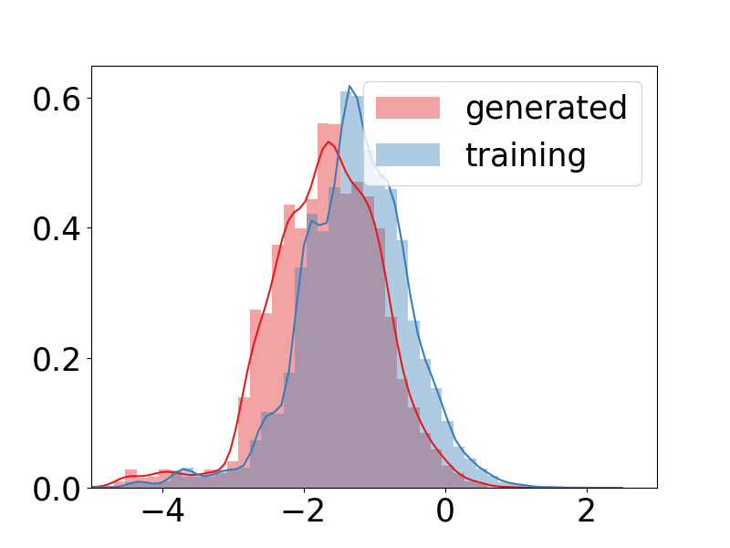
Mol weight	Drug-likeness

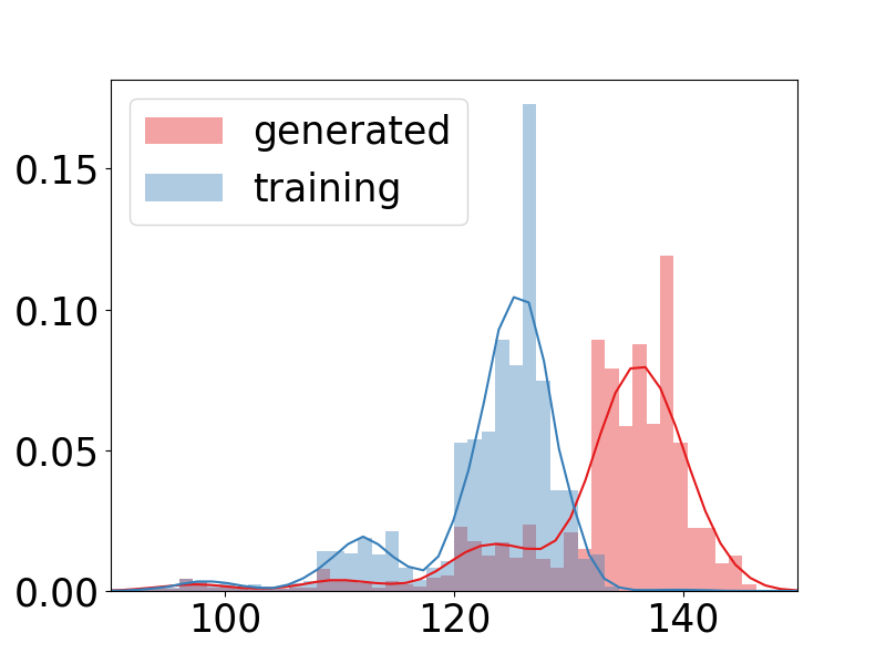
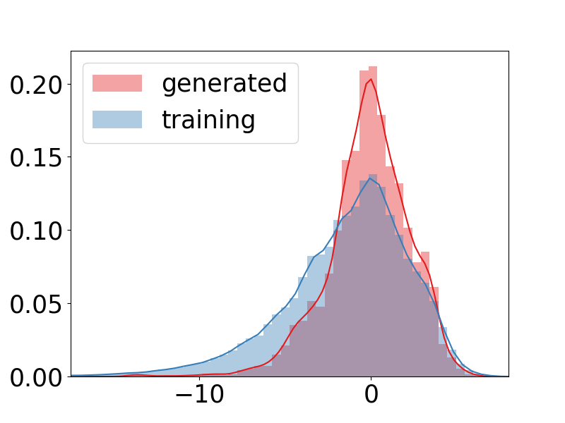
Figure 8: Comparison of the distribution of cLogP, cLogS, Molecular Weight, and Drug-likeness in the generated versus the training dataset for CGVAE). Results are better seen in color.

CGVAE
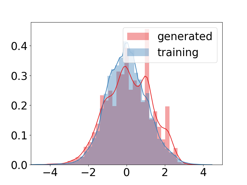
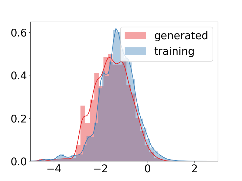
Mol weight	Drug-likeness
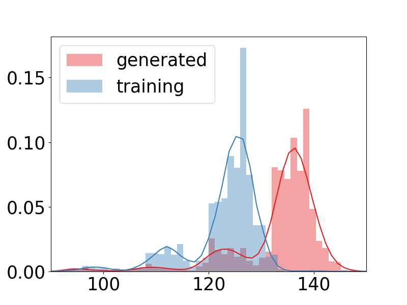
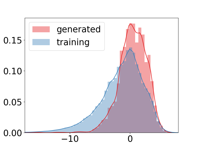
MDVAE
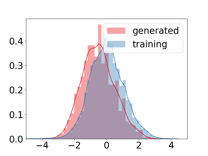
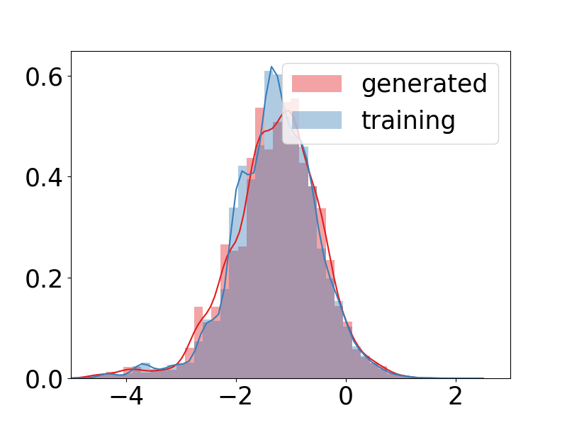
Mol weight	Drug-likeness

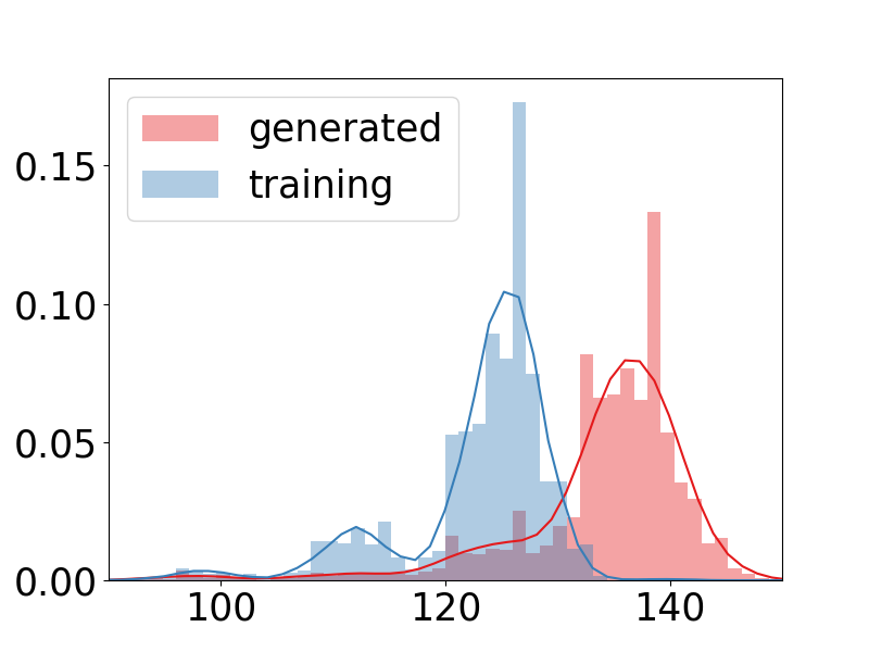
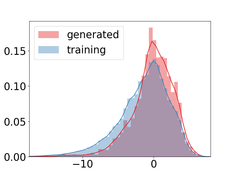
Figure 9: Comparison of the distribution of cLogP, cLogS, Molecular Weight, and Drug-likeness in the generated versus the training dataset for DVAE (top row), and MDVAE (bottom row). Results are better seen in color.

References

- [1] G. M. Whitesides. Reinventing chemistry. Angew Chem Int Ed Engl, 54(11):3196–209, 2015.
- [2] P. Schneider and G. Schneider. De novo design at the edge of chaos. J Medicinal Chem, 59(9):4077–4086, 2016.
- [3] D. Stumpfe and B. Bajorath. Similarity searching. Comput Mol Sci, 1(2):260–282, 2011.
- [4] Rafael Gómez-Bombarelli, Jennifer N Wei, David Duvenaud, José Miguel Hernández-Lobato, Benjamín Sánchez-Lengeling, Dennis Sheberla, Jorge Aguilera-Iparraguirre, Timothy D Hirzel, Ryan P Adams, and Alán Aspuru-Guzik. Automatic chemical design using a data-driven continuous representation of molecules. ACS central science, 4(2):268–276, 2018.
- [5] Matt J Kusner, Brooks Paige, and José Miguel Hernández-Lobato. Grammar variational autoencoder. In ICML, pages 1945–1954. JMLR. org, 2017.
- [6] Martin Simonovsky and Nikos Komodakis. Graphvae: Towards generation of small graphs using variational autoencoders. In International Conference on Artificial Neural Networks, pages 412–422. Springer, 2018.
- [7] Wengong Jin, Regina Barzilay, and Tommi Jaakkola. Junction tree variational autoencoder for molecular graph generation. arXiv preprint arXiv:1802.04364, 2018.
- [8] Mariya Popova, Mykhailo Shvets, Junier Oliva, and Olexandr Isayev. Molecularrnn: Generating realistic molecular graphs with optimized properties. arXiv preprint arXiv:1905.13372, 2019.
- [9] Paul D Leeson and Brian Springthorpe. The influence of drug-like concepts on decision-making in medicinal chemistry. Nature Reviews Drug Discovery, 6(11):881–890, 2007.
- [10] Marwin HS Segler, Thierry Kogej, Christian Tyrchan, and Mark P Waller. Generating focused molecule libraries for drug discovery with recurrent neural networks. ACS central science, 4(1):120–131, 2018.
- [11] Mario Krenn, Florian Häse, AkshatKumar Nigam, Pascal Friederich, and Alan Aspuru-Guzik. Self-referencing embedded strings (selfies): A 100% robust molecular string representation. Machine Learning: Science and Technology, 1(4):045024, 2020.
- [12] Hanjun Dai, Yingtao Tian, Bo Dai, Steven Skiena, and Le Song. Syntax-directed variational autoencoder for structured data. arXiv preprint arXiv:1802.08786, 2018.
- [13] David Janz, Jos van der Westhuizen, and José Miguel Hernández-Lobato. Actively learning what makes a discrete sequence valid. arXiv preprint arXiv:1708.04465, 2017.
- [14] Gabriel Lima Guimaraes, Benjamin Sanchez-Lengeling, Carlos Outeiral, Pedro Luis Cunha Farias, and Alán Aspuru-Guzik. Objective-reinforced generative adversarial networks (organ) for sequence generation models. arXiv preprint arXiv:1705.10843, 2017.
- [15] Qi Liu, Miltiadis Allamanis, Marc Brockschmidt, and Alexander Gaunt. Constrained graph variational autoencoders for molecule design. In NeurIPS, pages 7795–7804, 2018.
- [16] Bidisha Samanta, Abir De, Niloy Ganguly, and Manuel Gomez-Rodriguez. Designing random graph models using variational autoencoders with applications to chemical design. arXiv preprint arXiv:1802.05283, 2018.
- [17] Xiaojie Guo, Yuanqi Du, and Liang Zhao. Property controllable variational autoencoder via invertible mutual dependence. In ICLR, 2020.
- [18] Yuanqi Du, Xiaojie Guo, Amarda Shehu, and Liang Zhao. Interpretable molecule generation via disentanglement learning. In BCB, pages 1–8, 2020.
- [19] Yuanqi Du, Yinkai Wang, Fardina Alam, Yuanjie Lu, Xiaojie Guo, Liang Zhao, and Amarda Shehu. Deep latent-variable models for controllable molecule generation. In BIBM. IEEE, 2021.
- [20] Xiaojie Guo, Yuanqi Du, Sivani Tadepalli, Liang Zhao, and Amarda Shehu. Generating tertiary protein structures via interpretable graph variational autoencoders. Bioinformatics Advances, 2021.
- [21] Xiaojie Guo, Yuanqi Du, and Liang Zhao. Deep generative models for spatial networks. In SIGKDD, pages 505–515, 2021.
- [22] Yuanqi Du, Xiaojie Guo, Hengning Cao, Yanfang Ye, and Liang Zhao. Disentangled spatiotemporal graph generative model. In AAAI, 2022.
- [23] Aleksandar Bojchevski, Oleksandr Shchur, Daniel Zügner, and Stephan Günnemann. Netgan: Generating graphs via random walks. In ICML, pages 609–618, 2018.
- [24] Xiaojie Guo, Lingfei Wu, and Liang Zhao. Deep graph translation. arXiv preprint arXiv:1805.09980, 2018.
- [25] Taseef Rahman, Yuanqi Du, Liang Zhao, and Amarda Shehu. Generative adversarial learning of protein tertiary structures. Molecules, 26(5):1209, 2021.
- [26] Jiaxuan You, Rex Ying, Xiang Ren, William L Hamilton, and Jure Leskovec. Graphrnn: Generating realistic graphs with deep auto-regressive models. arXiv preprint arXiv:1802.08773, 2018.
- [27] Tianfan Fu, Cao Xiao, and Jimeng Sun. Core: Automatic molecule optimization using copy & refine strategy. In Proceedings of the AAAI Conference on Artificial Intelligence, volume 34, pages 638–645, 2020.
- [28] Tianfan Fu, Cao Xiao, Xinhao Li, Lucas M Glass, and Jimeng Sun. Mimosa: Multi-constraint molecule sampling for molecule optimization. In Proceedings of the AAAI Conference on Artificial Intelligence, volume 35, pages 125–133, 2021.
- [29] Tianfan Fu, Wenhao Gao, Cao Xiao, Jacob Yasonik, Connor W Coley, and Jimeng Sun. Differentiable scaffolding tree for molecular optimization. arXiv preprint arXiv:2109.10469, 2021.
- [30] Yuanqi Du, Shiyu Wang, Xiaojie Guo, Hengning Cao, Shujie Hu, Junji Jiang, Aishwarya Varala, Abhinav Angirekula, and Liang Zhao. Graphgt: Machine learning datasets for graph generation and transformation. In NeurIPS, 2021.
- [31] Aditya Grover, Aaron Zweig, and Stefano Ermon. Graphite: Iterative generative modeling of graphs. In ICML, volume 97, pages 2434–2444, 2019.
- [32] Thomas N Kipf and Max Welling. Variational graph auto-encoders. arXiv preprint arXiv:1611.07308, 2016.
- [33] Alexander A. Alemi, Ian Fischer, Joshua V. Dillon, and Kevin Murphy. Deep variational information bottleneck. In ICLR. OpenReview.net, 2017.
- [34] Tian Qi Chen, Xuechen Li, Roger B Grosse, and David K Duvenaud. Isolating sources of disentanglement in variational autoencoders. In NeurIPS, pages 2610–2620, 2018.
- [35] Irina Higgins, Loïc Matthey, Arka Pal, Christopher Burgess, Xavier Glorot, Matthew Botvinick, Shakir Mohamed, and Alexander Lerchner. beta-vae: Learning basic visual concepts with a constrained variational framework. In ICLR. OpenReview.net, 2017.
- [36] Hyunjik Kim and Andriy Mnih. Disentangling by factorising. arXiv preprint arXiv:1802.05983, 2018.
- [37] Babak Esmaeili, Hao Wu, Sarthak Jain, Alican Bozkurt, N Siddharth, Brooks Paige, Dana H Brooks, Jennifer Dy, and Jan-Willem van de Meent. Structured disentangled representations. JMLR, 89, 2019.
- [38] Abhishek Kumar, Prasanna Sattigeri, and Avinash Balakrishnan. Variational inference of disentangled latent concepts from unlabeled observations. In ICLR. OpenReview.net, 2018.
- [39] Shengjia Zhao, Jiaming Song, and Stefano Ermon. Infovae: Information maximizing variational autoencoders. In AAAI, 2019.
- [40] Emmanuel Noutahi, Dominique Beani, Julien Horwood, and Prudencio Tossou. Towards interpretable sparse graph representation learning with laplacian pooling. arXiv preprint arXiv:1905.11577, 2019.
- [41] Christopher M Bishop. Pattern recognition and machine learning. springer, 2006.
- [42] Abhishek Kumar, Prasanna Sattigeri, and Avinash Balakrishnan. Variational inference of disentangled latent concepts from unlabeled observations. arXiv preprint arXiv:1711.00848, 2017.
- [43] Ian Goodfellow, Yoshua Bengio, and Aaron Courville. Deep Learning. MIT Press, 2016. http://www.deeplearningbook.org.
- [44] Jiaxuan You, Bowen Liu, Zhitao Ying, Vijay Pande, and Jure Leskovec. Graph convolutional policy network for goal-directed molecular graph generation. In NeurIPS, pages 6410–6421, 2018.
- [45] Qi Liu, Miltiadis Allamanis, Marc Brockschmidt, and Alexander Gaunt. Constrained graph variational autoencoders for molecule design. In S. Bengio, H. Wallach, H. Larochelle, K. Grauman, N. Cesa-Bianchi, and R. Garnett, editors, NeurIPS 31, pages 7795–7804. Curran Associates, Inc., 2018.
- [46] Yujia Li, Oriol Vinyals, Chris Dyer, Razvan Pascanu, and Peter W. Battaglia. Learning deep generative models of graphs. CoRR, abs/1803.03324, 2018.
- [47] Martin Sundermeyer, Ralf Schlüter, and Hermann Ney. Lstm neural networks for language modeling. In INTERSPEECH, 2012.
- [48] Raghunathan Ramakrishnan, Pavlo O Dral, Matthias Rupp, and O Anatole Von Lilienfeld. Quantum chemistry structures and properties of 134 kilo molecules. Scientific data, 1:140022, 2014.
- [49] John J Irwin, Teague Sterling, Michael M Mysinger, Erin S Bolstad, and Ryan G Coleman. Zinc: a free tool to discover chemistry for biology. JCIM, 52(7):1757–1768, 2012.
- [50] Karl Ridgeway and Michael C Mozer. Learning deep disentangled embeddings with the f-statistic loss. In NeurIPS, pages 185–194, 2018.
- [51] Cian Eastwood and Christopher KI Williams. A framework for the quantitative evaluation of disentangled representations. 2018.
- [52] Francesco Locatello, Stefan Bauer, Mario Lucic, Gunnar Rätsch, Sylvain Gelly, Bernhard Schölkopf, and Olivier Bachem. Challenging common assumptions in the unsupervised learning of disentangled representations. ICML, 2018.