Disentangled Spatiotemporal Graph Generative Models

Abstract

Modeling and understanding spatiotemporal graphs have been a long-standing research topic in network science and typically replies on network processing hypothesized by human knowledge. In this paper, we aim at pushing forward the modeling and understanding of spatiotemporal graphs via new disentangled deep generative models. Specifically, a new Bayesian model is proposed that factorizes spatiotemporal graphs into spatial, temporal, and graph factors as well as the factors that explain the interplay among them. A variational objective function and new mutual information thresholding algorithms driven by information bottleneck theory have been proposed to maximize the disentanglement among the factors with theoretical guarantees. Qualitative and quantitative experiments on both synthetic and real-world datasets demonstrate the superiority of the proposed model over the state-of-the-art by up to 69.2% for graph generation and 41.5% for interpretability.

Introduction

Spatiotemporal graph represents a vital data structure where the nodes and edges are embedded and evolve in a geometric space. Nowadays, spatiotemporal graph data is becoming increasingly popular and important, ranging from epidemic, transportation to biological network modeling (dye2003modeling; ingraham2021generative; stopher1975urban; teng1985comparison). For example, the epidemic spreading network and the protein folding process can both be represented as spatiotemporal graphs, respectively. Spatiotemporal graphs cannot be modeled using either the spatial, graph, or temporal information individually, but require the simultaneous characterization of both the data and their interactions, which results in various patterns (barthelemy2011spatial). Spatial and graph aspects of information are usually correlated. For example, geographically nearby people tend to befriend in a social network. Moreover, the above interplay between spatial and graph aspects is a dynamic process, thus, the consideration in time aspect is inevitable for a comprehensive modeling. Recently, although spatiotemporal graph deep learning has stimulated a surge of research for graph representation learning (cui2019traffic; wu2019graph; yu2017spatio), however, deep generative models for spatiotemporal graphs have not been well explored.

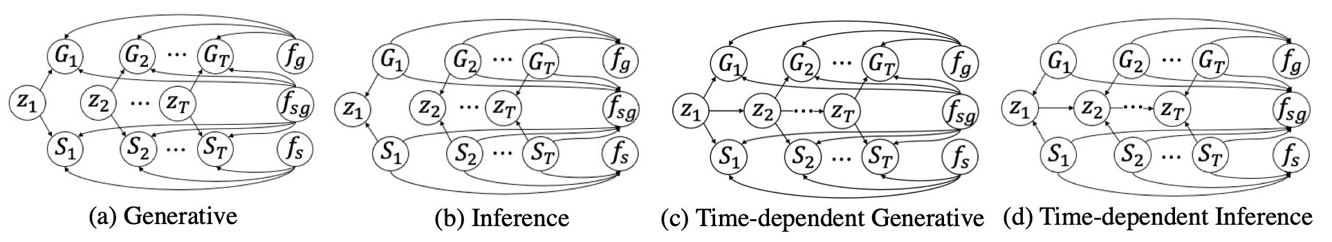
Figure 1: Graphical illustration of the proposed models.

Modeling and understanding the generative process of spatiotemporal graphs are a long-lasting research topic in domains such as graph theory and network science. Traditional methods usually extend and integrate network models in spatial networks (e.g., protein and molecule structures) and temporal graphs (e.g., traffic networks and epidemic spreading networks) into spatiotemporal graphs which captures some predefined properties of a graph, e.g., degree distribution, structure of community, clustering patterns. However, these models heavily rely on the predefined network process and rich knowledge of the graph properties, while the network properties and generation principles always remain unknown in the real-world applications, such as models that explain the mechanisms of mental diseases in brain networks during an activity of human beings and protein structure folding. Another line of research works is computational simulation models of spatiotemporal graphs customized for specific applications such as epidemics, brain simulator, and transportation simulation (dye2003modeling; stopher1975urban; teng1985comparison; guo2020generating; du2020interpretable; guo2020property; rahman2021generative). However, they are domain-specific with enormously detailed prior knowledge involved. This motivates us to propose the spatiotemporal graph models which can automatically learning the underlying spatial, temporal, and graph processes as well as their interplay.

In this paper, we propose, to the best of our knowledge, the first general deep generative model framework that models and disentangles spatiotemporal graph data. Specifically, we first propose a novel deep Bayesian network that factorizes spatiotemporal graphs into the time-variant, time-invariant, spatial-graph joint, and independent factors. A new objective driven by information-bottleneck theory has been proposed that can maximize the disentanglement of different factors as well as latent variables inside each factor, with theoretical guarantees. To optimize this objective function, a novel information-iterative-thresholding algorithm has been proposed to jointly optimize the objective and optimize its hyperparameters on information bottlenecks with theoretical analysis on optimal conditions. Extensive quantitative and qualitative experiments on two synthetic and two real-world datasets show the superiority of our proposed model over the state-of-the-art graph generative models by up to $69.2\%$ for spatiotemporal graph generation and $41.5\%$ for interpretability.

Methodology

Problem Formulation

A spatiotemporal graph is defined as $(S_{1:T},G_{1:T})$, where $T$ represents number of time frames of the spatiotemporal graphs, and $S_{1:T}=\{S_{1},S_{2},...S_{T}\},G_{1:T}=\{G_{1},...G_{T}\}$. $S_{t}=(\mathcal{V}_{t},C_{t})$ represents the geometric information of $t$-th snapshot of a spatiotemporal graph, where $\mathcal{V}_{t}$ denotes a set of $N$ nodes and $C_{t}\in\mathbb{R}^{N\times 3}$ denotes 3D geometric information. $G_{t}=(\mathcal{V}_{t},\mathcal{E}_{t},X_{t},E_{t})$ represents the graph information of $t$-th snapshot, where $\mathcal{E}_{t}\subseteq\mathcal{V}_{t}\times\mathcal{V}_{t}$ is the set of edges. $E_{t}\in\mathbb{R}^{N\times N\times K}$ refers to the edge weights or adjacent matrix, and $K$ refers to the edge feature dimension. $X_{t}\in\mathbb{R}^{N\times M}$ denotes the node feature and $M$ is the length of the node feature vector.

This paper aims at proposing a general data-driven framework for modeling spatiotemporal graphs, under fundamental, necessary factors. First, for any spatiotemporal graphs, there could be patterns that are time-variant and time-invariant. While time-invariant, spatial and graph information could either be correlated or independent, hence it is important to distinguish and capture these different semantic factors via different latent variables. More concretely, the goal is to learn a posterior $p(S_{1:T},G_{1:T}|Z,F)$ of the spatiotemporal graphs given four groups of generative latent variables $Z=z_{1:T}\in\mathbb{R}^{L_{1}}$ for time-variant features and $F=(f_{s}\in\mathbb{R}^{L_{2}},f_{g}\in\mathbb{R}^{L_{3}},f_{sg}\in\mathbb{R}^{L_{4}})$ for time-invariant features, where we need to capture and disentangle time-variant factors $z_{1:T}$, time-invariant geometric factors $f_{s}$, graph factors $f_{g}$ and spatial-graph joint factors $f_{sg}$. $L_{1}$, $L_{2}$, $L_{3}$, and $L_{4}$ are the number of variables in each group of factors, respectively. The encoding and generative process of our proposed SpatioTemporal Graph Disentangled Variational Auto-Encoder (STGD-VAE) model is illustrated in Fig. 1(a) and Fig. 1(b). Another implementation of the proposed model following the common time-dependency assumption, namely, STGD-VAE-Dep is illustrated in Fig. 1(c) and Fig. 1(d), and detailed in the appendix.

The Objective on Spatiotemporal Graph Generative Modeling

To learn the conditional probability $p(S_{1:T},G_{1:T}|z_{1:T},F)$, it is equal to maximizing the marginal likelihood of the observed spatiotemporal graph sequence $(S_{1:T},G_{1:T})$ in expectation over the distribution of the latent representation as $\mathbb{E}_{p_{\theta}(z_{1:T},F)}p_{\theta}(S_{1:T},G_{1:T}|z_{1:T},F)$. The prior distribution of the latent spaces is described as $p(z_{1:T},F)$ with the observation of a spatiotemporal graph sequence $(S_{1:T},G_{1:T})$, which, however, is intractable. Therefore, a variational objective is proposed to tackle this problem, where the posterior distribution is approximated by another distribution $q_{\phi}(z_{1:T},F|S_{1:T},G_{1:T})$. The objective can be written as minimizing the Kullback-Leibler Divergence (KLD) between the true prior distribution and the approximate posterior distribution. In order to encourage this disentanglement property of $q_{\phi}(z_{1:T},F|S_{1:T},G_{1:T})$, we introduce a constraint by trying to match the inferred posterior configurations of the latent factors to the prior $p(z_{1:T},f_{s},f_{g},f_{sg})$. This can be achieved if we set each prior to be an isotropic unit Gaussian, i.e., $\mathcal{N}(\textbf{0},\textbf{1})$, leading to a constrained optimization problem as:

$$\max_{\theta,\phi}\quad \mathbb{E}_{S_{1:T},G_{1:T}\sim\mathcal{D}}\mathbb{E}_{q_{\phi}(z_{1:T},F|S_{1:T},G_{1:T})}$$

$$\sum\nolimits_{t=1}^{T}[\log p_{\theta}(G_{t}|z_{t},f_{g},f_{sg})+\log p_{\theta}(S_{t}|z_{t},f_{s},f_{sg})]$$

s.t. $$\quad\sum\nolimits_{t=1}^{T}D_{KL}(q_{\phi}(z_{t}|S_{t},G_{t})||p(z_{t}))<I_{t}$$

$$\quad D_{KL}(q_{\phi}(f_{g}|G_{1:T})||p(f_{g}))<I_{g}$$

$$\quad D_{KL}(q_{\phi}(f_{s}|S_{1:T})||p(f_{s}))<I_{s}$$

$$\quad D_{KL}(q_{\phi}(f_{sg}|S_{1:T},G_{1:T})||p(f_{sg}))<I_{sg}$$

$$\quad I_{sg}\leq C_{sg},\quad I_{t}\leq C_{t}.$$ (1)

The detailed objective and proposed mutual information thresholding algorithm can be found in the appendix.

Experiments

Experiment Set-up

We validate the effectiveness of our proposed models on two synthetic datasets and two real-world datasets (du2021graphgt), (1) Dynamic Waxman Random Graphs, (2) Dynamic Random Geometry Graphs, (3) Protein Folding Dataset, and (4) Traffic Dataset MERT-LA. Despite no previous deep generative models specifically designed for spatiotemporal graph generation, we compare with some general graph generation models, including GraphRNN (you2018graphrnn), GraphVAE (kipf2016variational), and a traditional algorithm DSBM (xu2014dynamic). In terms of disentanglement evaluation, we also apply and compare with beta-VAE (higgins2016beta), beta-TC-VAE (chen2018isolating), and NED-IPVAE (guo2020interpretable) to our proposed method.

Table 1: The evaluation results for the generated spatiotemporal graphs for different datasets (KLD_cls refers to KLD of graph clustering coefficient. KLD_ds refers to KLD of graph density, KLD_bet refers to KLD of betweenness centrality, and KLD_tcorr refers to KLD of temporal correlation.

Dataset	Method	Node	Spatial	Edge	KLD_cls	KLD_ds	KLD_bet	KLD_tcorr	AvgMI
DWR Graph	DSBM	N/A	N/A	54.95%	0.90	1.10	0.63	0.73	N/A
	GraphVAE	0.57	0.57	57.14%	1.63	1.82	0.91	0.85	N/A
	GraphRNN	N/A	N/A	55.24%	1.97	2.50	1.00	1.35	N/A
	beta-VAE	0.0012	0.0011	69.05%	0.43	1.61	1.82	0.36	2.25
	beta-TCVAE	0.0013	0.0012	69.04%	0.47	1.37	1.56	0.08	2.33
	NEND-IPVAE	0.016	0.0008	65.80%	1.39	1.82	2.78	0.11	2.52
	STGD-VAE	0.0003	0.0001	69.99%	0.14	0.74	0.40	0.03	2.03
	STGD-VAE-Dep	0.0191	0.0005	66.28%	0.45	0.55	0.54	0.38	2.04
DRG Graph	DSBM	N/A	N/A	81.88%	1.77	2.87	3.38	0.64	N/A
	GraphVAE	0.56	0.74	85.75%	4.46	2.65	1.60	3.08	N/A
	GraphRNN	N/A	N/A	85.32%	0.57	1.24	2.40	0.85	N/A
	beta-VAE	0.0013	0.0017	91.75%	0.34	1.24	1.47	2.15	2.29
	beta-TCVAE	0.0018	0.0019	91.62%	0.52	1.58	1.46	2.38	2.24
	NED-IPVAE	0.0175	0.0018	89.84%	0.37	1.05	1.72	0.23	2.42
	STGD-VAE	0.0004	0.0015	91.88%	0.14	0.72	0.28	0.11	2.07
	STGD-VAE-Dep	0.0008	0.0017	91.28%	0.14	0.71	0.26	1.67	2.08
Protein	DSBM	N/A	N/A	70.78%	1.00	0.93	1.15	1.53	N/A
	GraphVAE	N/A	553.82	62.54%	1.26	1.44	1.48	1.90	N/A
	GraphRNN	N/A	N/A	71.17%	1.05	1.15	1.43	0.83	N/A
	beta-VAE	N/A	52.74	85.58%	0.16	0.14	0.46	0.61	1.04
	beta-TCVAE	N/A	35.05	95.80%	0.27	0.58	0.34	0.71	1.09
	NED-IPVAE	N/A	36.12	92.48%	1.08	0.79	0.44	2.64	1.15
	STGD-VAE	N/A	28.77	99.79%	0.33	0.21	0.53	0.23	0.70
	STGD-VAE-Dep	N/A	28.42	96.79%	0.13	0.54	1.55	0.24	0.76
Traffic	DSBM	N/A	N/A	N/A	N/A	N/A	N/A	N/A	N/A
	GraphVAE	N/A	N/A	N/A	N/A	N/A	N/A	N/A	N/A
	GraphRNN	N/A	N/A	N/A	N/A	N/A	N/A	N/A	N/A
	beta-VAE	7.15	N/A	N/A	N/A	N/A	N/A	N/A	1.37
	beta-TCVAE	8.50	N/A	N/A	N/A	N/A	N/A	N/A	1.18
	NED-IPVAE	31.95	N/A	N/A	N/A	N/A	N/A	N/A	1.18
	STGD-VAE	6.78	N/A	N/A	N/A	N/A	N/A	N/A	0.69
	STGD-VAE-Dep	5.13	N/A	N/A	N/A	N/A	N/A	N/A	1.06

Results

Quantitative Evaluation. We quantitatively evaluate the performance of our proposed model in two synthetic datasets and two real-world datasets by three types of evaluations, as shown in Table 1. We first evaluate the reconstruction via calculating the difference (e.g. mean sqaured errors) between the real graphs and the reconstructed graphs. Then, we evaluate the learnt graph property (i.e. (1) graph density, (2) average clustering coefficient, (3) betweenness centrality, and (4) temporal correlation) distribution comparing to the training one via Kullback-Leibler Divergence (KLD). Finally, we calculate the avgMI score (locatello2019challenging) which evaluates the disentanglement of the learnt latent space. We make several observations from the table. Firstly, STGD-VAE achieves the best overall results in the two synthetic datasets, both in reconstruction, distribution and disentanglement evaluation. Secondly, both STGD-VAE and STGD-VAE-Dep perform well in the two real-world datasets. Lastly, the proposed disentanglement of spatiotemporal graph factors greatly improve the disentanglement quality of the latent space.

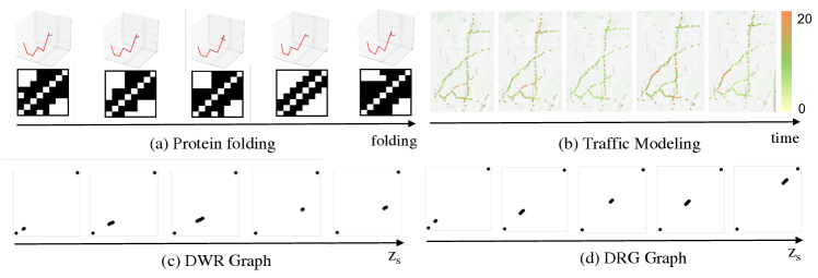
Figure 2: Qualitative evaluation on two synthetic datasets and two real-world datasets.

Qualitative Evaluation. As in the conventional qualitative evaluation in disentanglement representation learning (chen2018isolating; higgins2016beta), we change the value of one latent variable continuously while fixing the remaining variables to see the variation of the semantic factor it controls. In Fig. 2(a) and 2(b), we visualize the folding process of the protein structures and the traffic modeling process. We can observe that the residues on the right side are slightly folding up and moving towards left. For the traffic dataset, it is worth noting that the traffic speed is constantly changing in different time steps which reflects the real-time traffic situations. In Fig. 2(c) and 2(d), we also visualize the changes of the generated graphs when the latent factor $z_{s}$ of our STGD-VAE model change from $-5$ to $5$ in the dynamic Waxman random graph and the dynamic random geometry graph dataset, respectively. Clearly, the spatial location is changed accordingly, from the left-bottom corner to nearly the right-top corner, which shows that the latent variables learn and expose the semantic factors well.

Conclusion

In this paper, we introduce STGD-VAE and STGD-VAE-Dep, to the best of our knowledge, the first general deep generative model framework for spatiotemporal graphs. Specifically, we propose a new Bayesian model that factorizes spatiotemporal graphs into spatial, temporal, and graph factors as well as the factors that model the interactions among them. Moreover, a variational objective function and a new mutual information thresholding algorithm based on information bottleneck are proposed to maximize the disentanglement among the factors with theoretical guarantees. The comparison with several deep generative models validates the superiority of our proposed models from multiple tasks, including graph generation and disentangled representation learning. In the future, we plan to extend this framework to more types of sptiotemporal graphs.