Large-charge conformal dimensions at the $O(N)$ Wilson-Fisher fixed point

Abstract

Recent work using a large-charge expansion for the $O(N)$ Wilson-Fisher conformal field theory has shown that the anomalous dimensions of large-charge operators can be expressed in terms of a few low-energy constants (LECs) of a large-charge effective field theory (EFT). By performing lattice Monte Carlo computations at the $O(N)$ Wilson-Fisher fixed point, we compute the anomalous dimensions of large-charge operators up to $N=8$ and charge $Q=10$, and extract the leading and subleading LECs of the $O(N)$ large-charge EFT. To alleviate the signal-to-noise ratio problem present in the large-charge sector of conventional lattice formulations of the $O(N)$ theory, we employ a recently developed qubit formulation of the $O(N)$ nonlinear sigma models with a worm algorithm. This enables us to test the validity of the large-charge expansion and the recent large-$N$ predictions for the coefficients of the large-charge EFT.

I Introduction

Conformal field theories (cfts) are ubiquitous in physics. In condensed matter physics, they describe the critical behavior of materials at second-order phase transitions [1, 2], and in particle physics, they arise naturally as renormalization group (rg) fixed points of relativistic quantum field theories (qfts) [3, 4, 5]. Understanding cfts is therefore pivotal to understanding a wide range of physical phenomenon.

Despite their importance, cfts remain a challenge to study This is because, in general, cfts are strongly-coupled and it can be difficult to find a small parameter to do a perturbative expansion. Nonetheless, much progress has been made by exploiting “hidden” small parameters such as in the large-$N$ expansion [6], the $\epsilon$-expansion [7], or with non-perturbative techniques such as conformal bootstrap [8, 9]. In some cases, lattice field theory methods offer a completely non-perturbative method to compute properties of a cft numerically [10]. All these techniques have their limitations and provide a window into a potentially different regimes of the cft.

In the last few years, there has been progress using a new small parameter: the inverse of a global charge $Q$ [11, 12]. For theories with a global symmetry, we can study the theory in sectors of fixed global charge $Q$ and obtain an expansion in inverse charge $Q^{-1}$. The work of Ref. [11] showed that, in certain theories such as the $O(2)$ Wilson-Fisher (wf) cft, restricting to sectors of fixed global charge causes a spontaneous breakdown of the global symmetry, giving rise to Goldstone modes [13]. We can then write down a low-energy effective field theory (eft) for the Goldstone modes, where the higher-order operators are suppressed in powers of the inverse charge $Q^{-1}$. The eft description allows us to make several predictions about the behavior the theory in sectors of large global charge. This was also extended to non-Abelian symmetries such as $O(2n)$ in many recent studies [14, 15, 16, 17, 18, 19, 20, 21].

While efts encode information about symmetries and relevant degrees of freedom, they also involve low-energy constants (lecs) which are a priori unknown. This prevents a quantitative computation of many observables of interest. Ideally, we would like to be able to compute the lecs directly from the underlying theory. The only known general technique which enables such quantitative computations in field theories is numerical lattice field theory, typically using Monte Carlo (mc) methods. Since lattice mc computations can work directly with the underlying theory, they can also provide independent check of the eft methods.

This two-pronged approach is also commonly used, for example, in studies of quantum chromodynamics (qcd). Since the low-energy sector of qcd is strongly coupled, we can write down efts such as chiral perturbation theory or pionless eft [22], describing the physics of low-energy degrees of freedoms, with unknown lecs. One then computes the lecs from lattice qcd computations, which allows both a non-trivial test of the eft methods, as well as a way to turn the low-energy efts into a powerful quantitative tool.

It is conceivable that such an combined lattice and eft approach can also be used with large-charge efts to study strongly-coupled cfts, especially if a sign-problem free formulation of the cft on the lattice can be found. This approach was taken in the works of Refs. [23, 24, 25] for the $O(2)$ and $O(4)$ wf cfts. The authors tested the predictions of large-charge eft using lattice mc methods. In particular, a prediction of the large-charge eft for these models is that the conformal dimensions of leading charge-$Q$ operators admit an expansion in $Q^{-1}$,

$$D(Q)=c_{{3}/{2}}Q^{3/2}+c_{{1}/{2}}Q^{1/2}+c_{0}+O(Q^{-1/2}),$$ (1)

where $c_{{3}/{2}},c_{{1}/{2}},\dotsc$ are the unknown lecs. In Ref. [23], the authors used a lattice formulation of the $O(2)$ nonlinear sigma model (nlsm) to directly compute the conformal dimensions of the charged operators, using which they computed the lecs by fitting to Eq. 1. This idea was then applied to the $O(4)$ wf cft in Ref. [24]. Surprisingly, the authors observed that, in both these cases, the validity of the large-charge expansion seems to extend all the way down to very small charges $Q\sim 1$.

Given the success of the large-charge expansion for the $O(2)$ and $O(4)$ theories, one might wonder if this feature of the large-charge expansion persists for the $O(N)$ models with larger $N$ as well. Recently, the authors of Ref. [26], studied the $O(N)$ model in a combined large-charge and large-$N$ expansion. They showed that the expansion given in Eq. 1 can be obtained for $O(N)$ models as well. Further, they derived expressions for the large-charge eft coefficients $c_{{3}/{2}},c_{{1}/{2}}$ in the large-$N$ limit. However, a numerical test of the validity of the large-$N$ results was only available for small $N=2,4$.

In this work, we fill this gap by extending the approach of earlier works [24, 23] to study large-charge sectors of the $O(N)$ wf fixed point for larger $N$ using lattice mc techniques. Using efficient worm algorithms, we compute the conformal dimensions $D(Q)$ of leading charge-$Q$ operators of the $O(N)$ wf fixed point, up to $Q=10$ and $N=8$. Assuming the expansion given in Eq. 1, as predicted by Ref. [26], we extract the leading coefficients $c_{{3}/{2}}$ and $c_{{1}/{2}}$. This lets us test the validity of the large-charge expansion for larger $N$ and the predictions of the large-$N$ expansion. Our final results are summarized in Fig. 8 and LABEL:tab:results.

One of the interesting features of the analysis of Ref. [24] was the use of a “qubit” $O(4)$ model to avoid a sign problem with the traditional $O(N)$ lattice vector model in sectors of large charges. In Refs. [27, 28], we generalized their $O(4)$ model to $O(N)$ qubit models for arbitrary $N$, and provided evidence to show that these qubit $O(N)$ models have a second-order critical point in the $O(N)$ wf universality class for $N=2,3,4,6,8$ in three spacetime dimensions. Therefore, we can use the qubit model tuned to this critical point for studying the wf cft. From the perspective of lattice mc computations, these models are appealing since they admit a worldline representation as a model of $N/2$ (for $N$ even) colored, oriented loops. In such a worldline formulation, we can develop a worm algorithm which can sample configurations very efficiently and compute the correlation functions, even in the large-charge sectors. These models have also recently become interesting due to their potential for studying qfts on quantum computers [28, 29, 30, 27, 31, 32].

This paper is organized as follows. In Section II, we review aspects of the large-charge expansion for the $O(N)$ wf cft relevant to our work. In particular, we emphasize the results for the conformal dimensions of the leading charged operators. In Section III, we review the $O(N)$ qubit model developed in Ref. [28], which we shall use to compute the conformal dimensions of large-charge operators, and describe a Monte Carlo approach based on worm algorithm to efficiently compute the conformal dimensions. We discuss the results of lattice calculations and compare with analytic results from literature in Section IV. We summarize this work and present our conclusions in Section V.

II Large-Charge Expansion for the $O(N)$ Wilson-Fisher Fixed Point

II.1 Wilson-Fisher CFT

We can define the $O(N)$ wf cft as the continuum limit of a certain lattice model at a second-order critical point. For example, we may consider the the partition function $Z=\int\mathcal{D\phi}\ e^{-S_{L}}$ with the Euclidean lattice action

$$S_{L}=-\beta\sum_{\langle xy\rangle}\vec{\phi}_{x}\cdot\vec{\phi}_{y}$$ (2)

defined on a $D$-dimensional Euclidean lattice with periodic boundary conditions. Here, $\vec{\phi}_{x}\in{\mathbb{R}}^{N}$ is an $N$-component bosonic real scalar field constrained such that $|\vec{\phi}_{x}|=1$, the sum runs over all bonds $\langle xy\rangle$ between nearest-neighbor lattice sites $x$ and $y$, and $\beta$ is a coupling that we can tune to a critical point. The field $\vec{\phi}_{x}$ transforms in the fundamental representation of $O(N)$, so that this lattice action has a manifest global $O(N)$ symmetry.

In $D\geq 3$ spacetime dimensions, this lattice model is known to have a second-order critical point at $\beta=\beta_{c}$ (finite). This critical point describes the spontaneous breakdown of the global $O(N)$ symmetry down to $O(N-1)$. As we make $\beta$ large and positive, the fields align and the system transitions from a disordered, $O(N)$ symmetric phase into an ordered phase with broken $O(N)$ symmetry. In $D=4$ spacetime dimensions, the corresponding rg fixed point is the Gaussian fixed point, which just gives the free field theory in the continuum limit with logarithmic corrections. However, in $D=3$, this is a nontrivial fixed point called the wf fixed point [7]. The continuum limit at this critical point is an interacting conformally-invariant field theory, called the wf cft.

II.2 Large-charge expansion

Since the goal of this work is to obtain quantitative results on the $O(N)$ Wilson-Fisher cft and to connect with the large-charge expansion, let us briefly review the results of the large-charge expansion for the $O(N)$ model. We highlight the results which are relevant to our work and refer the reader to the original literature for details [14, 11, 26].

The question that concerns us here is: what is the conformal dimension $D(Q)$ of the leading primary operator in the $O(N)$ wfCFT with a given charge $Q$? For the Abelian $O(2)$ group, the charge $q$ of a operator $\mathcal{O}_{q}$ determines the transformation under an $O(2)$ rotation in the field space, parametrized by an angle $\theta$ as $\mathcal{O}_{q}\to e^{iq\theta}\mathcal{O}_{q}$. In the limit of large $Q$, the analysis of Refs. [26, 14, 11] shows that, the conformal dimensions $D(Q)$ admit an expansion in inverse powers of $Q$,

$$D(Q)=c_{{3}/{2}}Q^{3/2}+c_{{1}/{2}}Q^{1/2}+c_{0}+O(Q^{-1/2}),$$ (3)

where $c_{{3}/{2}},c_{{1}/{2}},c_{0},\ldots$ are some unknown coefficients.

This notion of a charge can be generalized to $O(2n)$ by fixing $n$ orthogonal planes and considering independent $O(2)$ rotations in each plane. This form the maximal torus subgroup of $O(2n)$. Let the $n$ independent $O(2)$ rotations be parameterized by angles $\vec{\theta}=(\theta_{1},\dotsc,\theta_{n})$, where $\theta_{i}$ parametrizes the $O(2)$ rotation in the $(2i-1,2i)$ plane. A operator $\mathcal{O}_{\vec{q}}$ with well-defined $O(2n)$ charges transforms as $\mathcal{O}_{\vec{q}}\to e^{i\vec{\theta}\cdot\vec{q}}\mathcal{O}_{\vec{q}}$ under the action of generators in the Cartan subgalebra, where we define the vector $\vec{q}=(q_{1},\dotsc,q_{n})$ as the charge of the operator $\mathcal{O}_{\vec{q}}$. In the large-charge expansion, the relevant quantity is $Q=\sum_{i}|q_{i}|$. With this definition of $Q$, the authors of Ref. [26] found that Eq. 3 holds for the $O(2n)$ theory as well.

The result in Eq. 3 is obtained from an eft analysis. In sectors of fixed non-zero global charge, the authors of Ref. [26] note that the global $O(2n)$ symmetry is explicitly broken to a $U(n)$ symmetry, which further undergoes a spontaneous breakdown to $U(n-1)$:

$$O(2n)\xrightarrow{\text{explicit}}U(n)\xrightarrow{\textsc{ssb}}U(n-1).$$ (4)

This is a slight generalization of the familiar scenario of spontaneous symmetry breaking (ssb) to sectors of fixed global charge, and indeed we find Nambu-Goldstone modes [13]. There are $(n-1)$ Goldstone bosons with a non-relativistic dispersion relation, and a single relativistic Goldstone boson. At low-energies, one can write down an eft description of the relativistic Goldstone boson, where the higher-order operators are suppressed by powers of inverse charge $Q^{-1}$.

Being an eft result, the lecs are unknown and depend on $N$. This is true for all the lecs except $c_{0}$, which is predicted to have a universal (independent of $N$) value of $c_{0}\approx-0.0937$. Recently, the combined large-$N$ and large-charge analysis of Ref. [26] predicted the coefficients $c_{{3}/{2}},c_{{1}/{2}}$ as functions of $N$,

$$c_{{3}/{2}}=(2/3)N^{-1/2},\quad c_{{1}/{2}}=(1/6)N^{1/2},$$ (5)

which should be valid in the regime $Q\ll N\ll Q^{2}$ for large $Q,N$.

Equations 3 and 5 are the focus of this work. We would like to develop a numerical mc method to accurately compute the conformal dimensions $D(Q)$, and test of validity of Eqs. 3 and 5 for the $O(N)$ theories over a wide range of $N$ and charge $Q$. We do this in the following sections.

III $O(N)$ Wilson-Fisher CFT from a qubit lattice model

III.1 Qubit $O(N)$ models

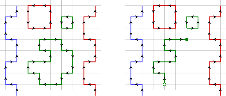
Figure 1: Typical worldline configurations contributing to partition function for the $O(6)$ qubit model in the default sector (left) and in the worm sector (right). The worldline representation for the $O(6)$ qubit model has 3 types of oriented worldlines, each representing a different $O(6)$ charge, which we show with different colors.

The $O(N)$ nlsm may be obtained as the continuum limit of the lattice action in Eq. 2. While there are efficient cluster algorithms for the traditional $O(N)$ model [33] for performing computations close to zero charge density, we are interested in numerical computations in sectors of large global $O(N)$ charges. In such cases, traditional mc approaches using the lattice action in Eq. 2 suffer from a sign problem.

In order to develop an efficient mc approach, we will instead use an $O(N)$ model with a finite-dimensional local Hilbert space, which we call a “qubit” $O(N)$ model. This model was constructed in a recent work [28] as an $O(N)$ generalization of the $N=2,3,4$ models studied in Refs. [34, 35, 24, 27]. The key point is that, in $(2+1)$ dimensions, this model has a second-order critical point in the $O(N)$ wf universality class. Therefore, we use this model at criticality to extract the conformal dimensions by measuring appropriate correlation functions.

Here, we quickly review the model and refer the reader to Ref. [28] for more details. The local (single-site) Hilbert space for the model is an $(N+1)$-dimensional space constructed as the direct sum of a singlet representation (which we think of as the empty “Fock vacuum” state) and an $N$-dimensional fundamental representation (which we think of as $N$ “particle” states) of the $O(N)$ group. The finite-temperature partition function of this model, $Z=e^{-\beta H}$, can be written as a worldline formulation in a manifestly spacetime symmetric way:

$$Z=\sum_{\mathcal{C}}W[\mathcal{C}],$$ (6)

where the sum is over worldline configurations $\mathcal{C}$ on a periodic Euclidean spacetime lattice, and $W[\mathcal{C}]$ is the weight of the configuration $\mathcal{C}$.

For the qubit $O(2n)$ model defined on a periodic spacetime lattice, we find that the configurations are composed of non-intersecting, closed, oriented worldlines of $n$ “colors.” An oriented worldline with color $i$ (where $i=1,\dotsc,n$) represents a state with $O(2n)$ charge $\vec{q}=\pm\hat{e}_{i}$ (where $\vec{e}_{i}$ is an $n$-vector with one at the $i$the position and $0$ elsewhere). That is, the color $i$ worldlines have charge $\pm 1$ under $O(2)$ rotations in the $(2i-1,2i)$ plane, and charge zero for rotations in all other planes. There are $n$ such worldlines, corresponding to the $n$ types of particles/anti-particle pairs transforming under the fundamental representation of $O(2n)$. For illustration, a typical configuration contributing to the partition function for the $O(6)$ model is shown in the left panel of Fig. 1, where we see oriented worldlines of 3 colors.

This spacetime symmetric model has only one parameter $U$, which is the weight of each bond between two sites. At $U=0$ there are no particles and the partition function is dominated by the trivial configuration with only singlets. At very large and positive $U$, the dominant contributions come from the $O(2n)$ particles, resulting in an $O(2n)$ symmetric ground state. However, in $3d$, we expect the $O(2n)$ symmetry of the ground state to be broken down to $O(2n-1)$. Therefore, as we tune $U$ from $0$ to $\infty$, this model goes to through a second-order phase transition at some $U=U_{c}$ which corresponds to the ssb scenario $O(2n)\to O(2n-1)$. This critical point was located precisely in Ref. [28], and confirmed to lie in the $O(2n)$ wf universality class by computing the critical exponents. Therefore, by tuning the model to this critical point $U=U_{c}$, we can study the physics of the wf fixed point.

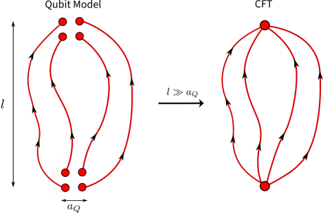
Figure 2: Computing the large-charge correlators of the cft from the qubit model. In the qubit model, we place $Q$ sources and sinks of a given color, each of unit charge, over a small region of linear size $a_{Q}$. In the limit of large separation $l\gg a_{Q}$, this computes the cft correlation function of the leading charge-$Q$ operators.

III.2 Conformal dimensions from the qubit $O(N)$ model

In this section, we describe a numerical mc method to compute the conformal dimensions of the charged operators. The method was introduced in Ref. [24] for the $O(4)$ model, but easily generalizes to the $O(N)$ case.

We are interested in the computing two-point correlators of the form

$$\langle\phi_{Q}(x)\ \phi_{-Q}(y)\rangle\sim|x-y|^{-2D(Q)}$$ (7)

where $\phi_{Q}$ is the leading primary operator with a charge $Q$, and $D(Q)$ is its conformal dimension. However, the qubit $O(N)$ model does not have single-site operators with charge $Q>1$. At any given site, the allowed charged states lie in the fundamental representation with $Q=1$.

We can work around this issue by appealing to scaling arguments. The charge-$Q$ correlators of the cft can be accessed in the qubit model by spreading $Q$ unit charges, say $\vec{q}_{1}=(1,0,\dotsc,0)$, over a small region to construct a smeared charge-$Q$ excitation over that region. To be concrete, let $\hat{\phi}_{L}(x)$ be any single-site lattice operator with charge $\vec{q}_{1}$ at the spacetime site $x$. Let $x_{1},\dotsc,x_{Q}$ be $Q$ spacetime points all within a radius $\sim a_{Q}$ of the point $x$. We define a product of lattice operators

$$\Phi_{Q}^{L}(x)=\phi^{L}(x_{1})\cdots\phi^{L}(x_{Q}),$$ (8)

which has a well-defined $O(2n)$ charge $\vec{q}=(Q,0,\dotsc,0)$. At criticality, the long-distance behavior of the two-point function of the lattice operators $\langle\Phi_{Q}^{L}(x)\Phi_{-Q}^{L}(y)\rangle$ gets a dominant contribution from the two-point function of the leading primary charge-$Q$ operators,

$$G_{Q}(x,y)=\langle\Phi_{Q}^{L}(x)\Phi_{-Q}^{L}(y)\rangle \sim|x-y|^{-2D(Q)},$$ (9)

in the limit $|x-y|\gg a_{Q}$. This is shown schematically in Fig. 2. Since we are interested only in the universal exponent of the leading power-law term, the exact form of the smearing does not matter.

III.3 Sketch of the Monte Carlo method

We would like to now develop an mc algorithm to measure correlators of the form in Eq. 9, in the presence of charged sources and sinks. We begin by defining a partition function for worldline configurations in a given charge sector,

$$Z_{Q}(L)=\sum_{\mathcal{C}_{Q}}W[\mathcal{C}_{Q}],$$ (10)

where we have explicitly specified the dependence on the system size $L$, and the sum is over worldline configurations $\mathcal{C}_{Q}$ having $Q$ sources and sinks placed in a specific manner as follows. Our model is manifestly spacetime symmetric, but we arbitrarily label one of the directions as time for convenience, and denote a spacetime point by $(t,\vec{x})$, where $\vec{x}$ is a spatial site on the time slice $t$. Let $L_{T}$ be the extent of the box in the time direction. We use sources and sinks of the same charge, say, $\vec{q}_{1}=(1,0,\dotsc,0)$. On the $t=0$ time slice, we place $Q$ sources in a small region close to $\vec{x}=0$, and on the $t=L_{T}/2$ time slice, we place $Q$ sinks around the site $\vec{x}=0$.

The exact placement of the charges does not matter in the scaling regime. However, the spread of these charges does introduce a short distance scale $a_{Q}\sim\sqrt{Q}$ in the system. Therefore, we choose the placement to have the smallest spread $a_{Q}$ possible. We show our choice in Fig. 3, where each circle shows a site with a unit charge $\vec{q}_{1}$, and the number showing the order in which these charges are placed as we increase the total charge of the system $Q$. As long as we have large separation between the sources and sinks, $l=L_{T}/2\gg a_{Q}$, we expect the universal power-law decay of the cft to emerge. (Note that for configurations contributing to $Z_{Q}$, we leave the site $\vec{x}=0$ empty on the both on the source and sink time slices. This special site will be used in an additional step below.) A typical configuration contributing to $Z_{Q}$ is shown in Fig. 4, in the $Q=2$ sector.

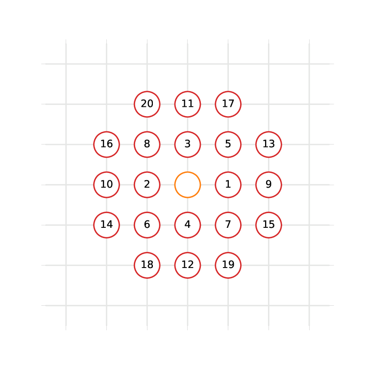
Figure 3: Placement of the sources and sinks for $Z_{Q}$ at the two-dimensional spatial slices $t=0$ and $t=L_{T}/2$. Each circle denotes a source (at $t=0$) or a sink (at $t=L_{T}/2$) of charge $\vec{q}_{1}=(1,0,\dotsc,0)$. The numbers denote the order in which we place these charges as we increase the total charge $Q$. For example, the charge placement shown in this figure corresponds to $Q=20$. The central site (corresponding to $\vec{x}=0$) is left empty for $Z_{Q}$, but is used in when adding an additional charge for the measurement update while sampling $\tilde{Z}_{Q+1}^{(\vec{x},t)}$.

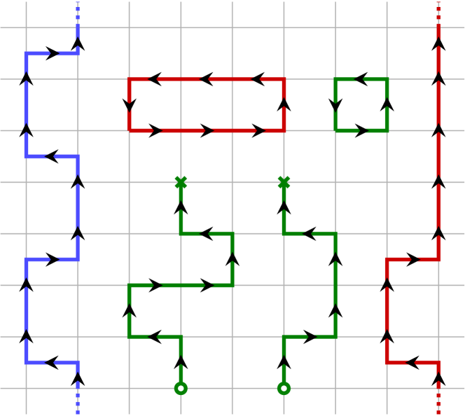
Figure 4: A typical worldline configuration for the $O(6)$ model with three colors, and two sources and sinks for green worldlines. The open circles indicate sources, and the crosses indicate sinks. The site between the two source sites is left empty as it is used in the measurement update.

Let us now define another partition function $\tilde{Z}_{Q+1}^{(t,\vec{x})}(L)$ in the charge $(Q+1)$ sector in the following way. The first $Q$ sources and sinks are placed in exactly the same way as for $Z_{Q}$ specified above. However, now there is an additional source at the spacetime site $(0,\vec{0})$ and a sink at the arbitrary site $(t,\vec{x})$. Finally, we define an extended partition function,

$$Z_{M}=Z_{Q}+\sum_{(t,\vec{x})}\tilde{Z}_{Q+1}^{(t,\vec{x})}.$$ (11)

We will describe, in Section III.4, a worm algorithm which can efficiently sample configurations in $Z_{M}$ by switching between the $Z_{Q}$ and $\tilde{Z}_{Q+1}^{(t,\vec{x})}$ sectors. This lets us compute the ratio of partition functions

$$R_{Q}(L)=\frac{\tilde{Z}_{Q+1}^{(L/2,\vec{0})}(L)}{Z_{Q}(L)}.$$ (12)

In the scaling limit $L\gg a_{Q}$, the ratio $R_{Q}$ in fact computes the ratio of two-point correlators of leading charge-$(Q+1)$ and charge-$Q$ operators,

$$R_{Q}(L)\sim\frac{G_{Q+1}(L/2)}{G_{Q}(L/2)}=cL^{-2\Delta(Q+1)},$$ (13)

where we have defined $\Delta(Q)$ as the difference of conformal dimensions

$$\Delta(Q)=D(Q)-D(Q-1).$$ (14)

We can therefore measure $D(Q)$ for any $Q$ by doing a series of computations for different charge sectors to measure $\Delta(Q)$ and computing,

$$D(Q)=\sum_{q=1}^{Q}\Delta(q).$$ (15)

where we set $D(0)=0$.

III.4 Details of the worm algorithm

We can now construct an efficient worm algorithm to sample the partition function [36, 37]. The full algorithm is composed of 3 sectors, where a different partition function is sampled, shown schematically in Fig. 5. The first is the “default” sector, given by Eq. 10, which consists of configurations in a given charge sector $Q$. We show an example of such a configuration in the left panel of Fig. 1. This is where we begin the algorithm. The other two sectors are the “worm” sector $Z_{Q,w}$ and the “measurement” sector $\tilde{Z}_{Q+1}$. Starting in the default sector $Z_{Q}$, we propose to either perform a worm update (sampling $Z_{Q,w}$), or to perform a measurement update (sampling $\tilde{Z}_{Q+1}$). The worm update is used to generate new configurations in $Z_{Q}$, and the measurement update is used to measure the observable $R_{Q}$ defined in Eq. 12. We now describe each of the updates.

Worm update: From the default sector, we first propose to move into the “worm” sector, where the partition function $Z_{Q,w}$ is sampled. The configurations contributing to $Z_{Q,w}$ are the same as $Z_{Q}$, except that they also include a single insertions of a creation and an annihilation operator of the same color at any two spacetime sites. For an example of such a worm configuration, see the right panel of Fig. 1. The key point is that worm algorithms can sample such configurations very efficiently [36, 37, 38]. For the zero-charge sector, the details of the worm algorithm used here were described in Refs. [27, 28]. Since we are working in sectors with fixed charge insertions, we modify the algorithm slightly to account for that.

The worm algorithm works by introducing a creation and annihilation operator at a random spacetime site to a configuration in $Z_{Q}$. As the worm head moves, it can either create a bond (if it moves towards an empty site), delete a bond (if it moves back on itself), or move a bond (if it moves into an existing worldline). The probability of each move is chosen such that the reverse move satisfies detailed balance. To account for the presence of charged operator insertions (sources and sinks), whenever a proposed move takes the worm head to one of the operator insertions, we simply reject the move. This ensures that only configurations with a fixed source/sink pattern are sampled. Once the worm head touches the worm tail, the worm update ends and we are back in the default sector.

Measurement update: From default sector $Z_{Q}$, we then propose to move into the “measurement sector,” where partition function $Z_{M}$, defined in Eq. 11, is sampled. This is a worm update very similar to the one defined above, except that we always begin by inserting the worm head/tail at the site $(0,\vec{0})$, instead of a random spacetime site. This site does not contain any sources, by construction of $Z_{Q}$. As the worm head moves, it samples configurations contributing to $\tilde{Z}_{Q+1}=\sum_{(t,\vec{x})}\tilde{Z}_{Q+1}^{(t,\vec{x})}$. Whenever the worm head touches the spacetime site $(L_{T}/2,\vec{0})$, we count that as a contribution towards $\tilde{Z}_{Q+1}^{(L_{T}/2,\vec{0})}$. In a given measurement update, let the number of configurations generated in $\tilde{Z}_{Q+1}^{(L_{T}/2,\vec{0})}$ be denoted by $N_{Q+1}$. The average of $N_{Q+1}$ over a large number of measurement updates computes precisely the observable $R_{Q}$ defined in Eq. 12,

$$\langle N_{Q+1}\rangle\approx R_{Q}=c|L_{T}|^{-2\Delta(Q+1)}.$$ (16)

Therefore this observable gives direct access to $\Delta(Q+1)$. We can repeat this computation over a range of $Q=0,1,\dotsc,Q_{\text{max}}$ and compute the conformal dimensions $D(Q)$.

As we increase the lattice size $L$, this algorithm can exhibit a signal-to-noise ratio problem in the measurement sector. This is because for large lattices, it becomes increasingly unlikely for the measurement worm head to touch the special site $(\vec{0},L_{T}/2)$ before closing. To improve the statistics, following Ref. [24], we also perform a reweighting of the worm configurations in $\tilde{Z}_{Q+1}$. If the worm tail is at $(0,\vec{0})$ and the worm head is at $(t,\vec{x})$, we multiply the weight of the worm configuration by $t^{p}$, where $p>0$ is chosen empirically. This makes it easier for the worm to grow very large and increases the likelihood that it touches $(L_{T}/2,\vec{0})$. It is easy to satisfy detailed balance with this reweighting and it improves the signal-to-noise ratio for the measurement update.

Figure 5: The full worm algorithm for the extraction of conformal dimensions of charge-$Q$ operators. We begin in the default sector $Z_{Q}$, defined as the sum over worldline configurations with $Q$ sources and sinks, each of charge $\vec{q}_{1}$, placed at time slices $t=0$ and $t=L_{T}/2$ as shown in Fig. 3. We perform worm updates to sample $Z_{Q,w}$, which consists of worldline configurations with an additional source and sink (worm tail and head). When the worm update ends, we obtain a new configuration in $Z_{Q}$. We then perform a measurement update by proposing to enter $\tilde{Z}_{Q+1}$. This is a special worm update of fixed color ($\vec{q}_{1}$) where the worm tail (source) is placed at $(0,\vec{0})$. When this update ends, we obtain a new measurement for the observable $R_{Q}$, defined in Eq. 12.

IV Results

In this section, we describe our results for the conformal dimensions of leading charge-$Q$ operators for the $O(N)$ wf cft for $N=2,4,6,8$ and over a range of $Q$, and compare with analytic predictions.

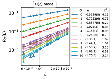
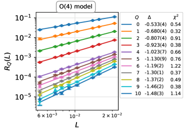
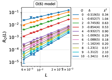
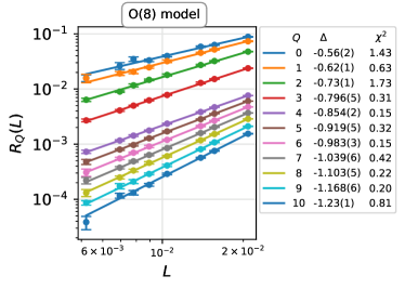
Figure 6: Extraction of conformal dimensions for the charge-$Q$ operators in the $O(N)$ model with $N=2,4,6,8$. The solid circles show the lattice mc data for the ratio $R_{Q}(L)$, defined in Eq. 12. The solid lines are fits to a power-law $R_{Q}(L)=cL^{-\Delta(Q+1)}$.

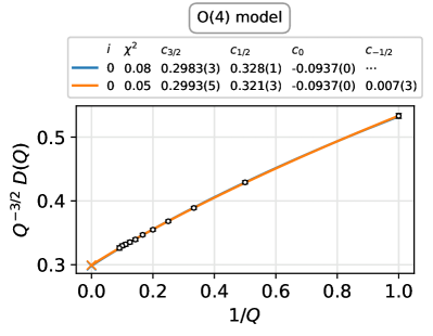
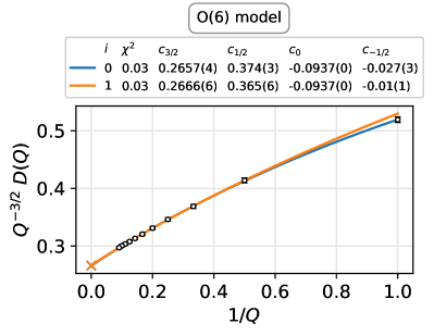
Figure 7: Extraction of the large-charge eft coefficients from $Q=1,\cdots,10$. We show the results for the $O(N)$ model with $N=2,4,6,8$. With $Q^{-3/2}D(Q)$ on the $y$-axis, and $Q^{-1}$ on the $x$-axis, the large-charge eft prediction is that the $x$-intercept is $c_{{3}/{2}}$ and the slope at the origin gives $c_{{1}/{2}}$. The curvature in the data is from the higher order terms ($c_{0}$ and higher-order) in the large-charge expansion. The small curvature indicates that the large-charge expansion is in fact quite accurate even for very low charge $Q$. We perform various fits by excluding the smallest $i$ charges data-points charges to estimate the systematic errors, until $\chi^{2}/\text{DOF}$ becomes small. An ellipsis ($\cdots$) in the columns for coefficient $c_{k}$ indicates that $c_{k}$ was not included in the fit, and an error of 0 (for $c_{0}$) indicates that the value of this parameter was fixed.

IV.1 Extraction of conformal dimensions

Given a $Q$ and $N$, we perform computations in the charge-$Q$ sector as described in the previous section and compute the observable $R_{Q}(L)$ defined in Eq. 12. We perform fits of the data to the form

$$R_{Q}(L)=c_{Q}L^{-2\Delta(Q+1)}$$ (17)

where $c_{Q}$ is a non-universal constant and $\Delta(Q)$ is the difference of conformal dimensions defined in Eq. 14. For each $N$, we compute $\Delta(Q)$ for $Q=1,\dotsc,10$. The conformal dimension $D(Q)$ of the leading charge-$Q$ operator is then extracted by just adding up the differences: $D(Q)=\sum_{q=1}^{Q}\Delta(Q)$. In Fig. 6, we show plots of $R_{Q}(L)$ as a function of $L$ for the $O(N)$ models with $N=2,4,6,8$. Although we find that statistical errors increase slightly with larger $Q$, the data is still precise enough to allow for a clean extraction of the exponent $\Delta(Q)$.

IV.2 Extraction of lecs of the large-charge eft

We rewrite the prediction for $D(Q)$ from the large-charge eft, Eq. 3, as

$$f(Q^{-1}) \equiv Q^{-3/2}D(Q)$$ (18)

$$=c_{{3}/{2}}+c_{{1}/{2}}Q^{-1}+c_{0}Q^{-3/2}+O(Q^{-2}).$$ (19)

The data for $f(Q^{-1})=Q^{-3/2}D(Q)$ as a function of $Q^{-1}$ should be linear close to $Q^{-1}=0$. Therefore, close to the origin we can perform a linear fit to extract the leading coefficients $c_{{3}/{2}},$ and $c_{{1}/{2}}$. We can also include higher-order terms to get an estimate of systematic errors in the fit. In Fig. 7, we show the data and fits for all the $O(N)$ models considered in this paper ($N=2,4,6,8$). We plot $Q^{-3/2}D(Q)$ vs. $Q^{-1}$ and perform fits of this data to the form

$$f(x)=c_{{3}/{2}}+c_{{1}/{2}}x^{1}+c_{0}x^{-3/2}+\sum_{k=2}^{k_{\text{max}}}c_{\nicefrac{{3}}{{2}}-k}x^{k}$$ (20)

where the power-series is cut off at $k=k_{\text{max}}$.

We note that the very small curvature of the data in Fig. 7 indicates that the large-charge expansion is quite accurate even at low charge $Q$, and therefore low values of $k_{\text{max}}$ are sufficient to obtain a very good fit. In other words, $c_{0}$ and higher order coefficients are quite small. Since it is not a priori clear which values of $Q$ should be included in the fits, we perform various fits for the total charge in a window $Q\in[Q_{\text{min}},Q_{\text{max}}]$. We fix $Q_{\text{max}}=10$ and vary $Q_{\text{min}}$ over a small range. As can be seen from the fits, even very small $Q$ seem to be described well by the “large-charge” expressions. This is an intriguing phenomenon that was also observed by Refs. [23, 24] for the $O(2)$ and $O(4)$ models. As evidenced by Fig. 7, this observation continues to hold for larger $N$, which is interesting.

We also vary the truncation order $k_{\text{max}}$ to get a sense of the systematics. As might be expected, we find that excellent fits are obtained already with $k_{\text{max}}\sim 2$ for most cases.

Figure 8: The two leading coefficients $c_{{3}/{2}}$ and $c_{{1}/{2}}$ in the large-charge expansion for the $O(N)$ Wilson-Fisher cft, shown as a function of $N$. The dotted lines show the large-$N$ predictions from Ref. [26]. The dark filled circles show the results of this work. The unfilled squares show the values of the lecs obtained in Refs. [23, 24] for $N=2,4$. We find that the $c_{3/2}$ prediction is in excellent agreement with lattice mc for $N\geq 6$. However, the subleading coefficient $c_{1/2}$, while within $\sim 3\sigma$ for $N\geq 6$, seems to be in mild tension. Regardless, large-$N$ correctly predicts the qualitative trends for both couplings.

IV.3 Comparison with large-charge and large-$N$ results

Finally, having extracted the lecs of the large-charge eft ($c_{{3}/{2}},c_{{1}/{2}},\dotsc$), we can compare the results against the large-$N$ predictions [39] as well as earlier lattice calculations [24, 23]. We show this comparison in Fig. 8 and LABEL:tab:results. The solid lines are predictions from a large-$N$ prediction of Ref. [26], while the results for $O(2)$ and $O(4)$ from previous lattice calculations [24, 23]. We also show the comparison with the earlier literature on the extraction of these couplings.

First, we note that the qualitative prediction of large-$N$ that $c_{{3}/{2}}$ decreases with $N$ while $c_{{1}/{2}}$ increases is in excellent agreement with the lattice data. Large-$N$ predicts that the two couplings are equal ($c_{{3}/{2}}=c_{{1}/{2}}$) at $N=4$. Interestingly, we find this to be true for the lattice results as well, although the actual numerical value of these couplings from large-$N$ differs from lattice by $\sim$\mathrm{1}\mathrm{0}${\%}$ at $N=4$.

On the quantitative side, we find that the leading coupling $c_{{3}/{2}}$ seems to be in beautiful agreement with large-$N$ already by $N=6$. On the other hand, the precise numbers for subleading coupling $c_{{1}/{2}}$ suggest some mild tension. Being a higher-order coupling, the error bars are larger as well. The source for this discrepancy could be either that large-$N$ takes longer to converge for the subleading coupling, or simply that the lattice computations need to be performed at higher precision. At this stage, it is hard to draw any quantitative conclusions for $c_{{1}/{2}}$. It is interesting that the authors of Ref. [26] also noted a small puzzle regarding the subleading coupling $c_{{1}/{2}}$, which might relate to this discrepancy as well.

We also compare with the values of the couplings obtained in the literature and find excellent agreement. For $N=2$, the couplings were obtained in Ref. [23] using the traditional lattice $O(2)$ model. Their model was substantially different from ours, therefore our results provide an independent verification of their work. As can be seen in Fig. 8, both the leading and subleading couplings agree within $\sim 2\sigma$. For $N=4$, our technique is quite similar to the one used in Ref. [24], where the authors also used a qubit $O(4)$ model. While the agreement is expected, the qubit model used in Ref. [24] differs slightly from the one used here. In particular, their model allowed a bond to ‘turn back on itself’, whereas in our model there are no such ‘double bonds.’ Since we are working at the criticality, such details are not expected to matter. This is indeed what we find. In both these cases ($N=2,4$), our results agree with and improve over the previous results.

Finally, we remark that the next-higher-order coupling $c_{0}$ is predicted to have a precise value from the large-charge expansion. However, being higher order, it is very tricky to extract from the precision obtained in this work. While it would be quite satisfying to extract the coupling $c_{0}$ numerically, in this work, we simply fixed it to the predicted value and let the other couplings vary.

[ label = tab:results, caption = Results for the large-charge expansion coefficients extracted from lattice Monte Carlo runs this work. We also include the numbers for the $O(2)$ and $O(4)$ models from literature. , mincapwidth=center, star, ] l S S S S @ S S S S S[a]Ref. [23], traditional lattice $O(2)$ model [b]Ref. [24], qubit $O(4)$ model [c]Ref. [26], combined large-$N$ and large-charge expansion& $c_{{3}/{2}}$ $c_{{1}/{2}}$ $N$ 2 4 6 8 2 4 6 8 This work 0.3429(5) 0.3013(4) 0.265(5) 0.228(2) 0.242(2) 0.302(3) 0.36(1) 0.44(1) Large-N[c] 0.471 0.333 0.272 0.236 0.236 0.333 0.408 0.471 Literature 0.337(3)[a] 0.301(1)[b] - - 0.27(1)[a] 0.29(1)[b] - -

V Conclusions

To explore the validity of the large-charge expansion for the $O(N)$ wf cft, we performed lattice mc computations for the $O(N)$ model at $N=2,4,6,8$. In order to avoid a signal-to-noise ratio problem as we go to higher charges, we used a qubit $O(N)$ model, which was shown recently to have a second-order critical point in universality class of the $O(N)$ wf fixed-point [28]. This model allows for efficient lattice computations using a worldline formulation with a worm algorithm, and allows precise extraction of the conformal dimensions up to $Q=10$ and $N=8$.

Having computed the conformal dimensions, we then performed a fit to the prediction from the large-charge eft and extracted the two leading lecs $c_{{3}/{2}}$ and $c_{{1}/{2}}$. In line with what the authors of Refs. [23, 24] observed for the $N=2,4$ models, we find that the large-charge expansion describes the data very well even for very small $Q$ for larger $N$ as well. This is an intriguing fact about the large-charge expansion which would be nice to understand theoretically.

We finally compared our numerical results for the lecs with a recent prediction from a combined large-charge and large-$N$ expansion [26]. We find that the large-$N$ prediction for the leading coefficient $c_{{3}/{2}}$ agrees very well with the numerical computations already for $N\geq 6$. The qualitative trends for both the leading lecs $c_{{3}/{2}},c_{{1}/{2}}$ are also predicted correctly by the large-$N$ expansion. However, there seems to be a small tension between numerical values and large-$N$ for the subleading coefficient $c_{{1}/{2}}$. This can be either due to the fact that subleading coefficient is harder to extract numerically and there might be unresolved systematics, or it could be that we just need to go to larger $N$ for the subleading coefficient. The authors of Ref. [26] also note a small puzzle regarding the $c_{{1}/{2}}$ coupling, which might be related to this issue. This merits further study and is left for a future publication.

Appendix A Exact calculations on a small lattice

In this section, we test our mc code by comparing against exact results for a small lattice. We consider a $2d$ spacetime lattice with $L=2$ and $L_{T}=4$, where all possible configurations can be easily enumerated. We put exactly one source and sink of a fixed color. In this case, there are exactly three types of configurations, as shown in Fig. 9.

Let the spacetime sites be indexed by integers $(x,t)$ where $x\in[0,1]$ and $t\in[0,3]$. We place one source of a given color (say, red) at the site $(0,0)$ and a sink of the same color at $(0,2)$. In Fig. 9, the sources are shown by a circles and the sinks are shown by a cross. In our setup, the first outgoing bond from the sources is always frozen to be in the positive time direction, so that the outgoing bond always points up, and the incoming bond for the sinks is frozen to be coming in from negative time direction, so that the bond always comes in from below. On this $2\times 4$ lattice, this completely freezes the worldline connecting the source and the sink. Therefore, we can easily enumerate all the allowed configurations in this system, as shown in Fig. 9. The first configuration shown has a single worldline of a fixed color and orientation since it connects a source with a sink, whereas the two configurations shown to its right have an additional worldline which can be of any of the $n$ colors and two orientations (so there are such $N=2n$ configurations). The weight of each configuration is given by multiplying the weight of each temporal bond, $W_{t}$, and each spatial bond $W_{s}$. Therefore the partition function in the charge-$1$ sector is

$$Z_{1}=W_{t}^{2}+NW_{t}^{6}+NW_{t}^{2}W_{s}^{2}.$$ (21)

We show results for the singlet density computed from the lattice mc algorithm against exact results in LABEL:tab:results-exact.

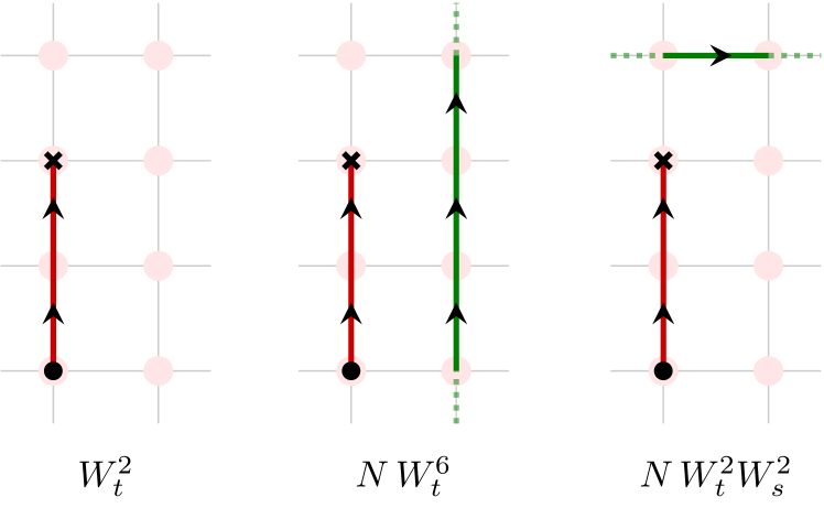
Figure 9: All the possible configurations with their weights on a $2d$ lattice of size $L=2$ and $L_{T}=4$ in the charge-$1$ sector. Here, we denote the weight of a temporal bond is $W_{t}$ and $W_{s}$ for clarity, although in our computations we have $W_{t}=W_{s}$. The dark circle represents a source and the cross represents a sink for the red worldlines. In our code the outgoing bonds at sources and incoming bonds at sinks are fixed to be in the temporal direction, so this completely fixes the red worldline on this small lattice. The other worldline can be of any color and orientation and contributes a factor of $N$ to the weights and second and third configurations.

[label = exact_results, caption = Comparison of the worm algorithm with exact calculations on a small $2\times 4$ lattice in the charge-$1$ sector. We show results for the “singlet density” observable, for various $N$, spatial weights ($W_{s}$) and temporal weights ($W_{t}$). We find complete agreement between the exact results and the worm algorithm. All the configurations contributing to this computation are shown in Fig. 9. , label = tab:results-exact, mincapwidth = center,]S S S S[table-format=1.7] S[table-format=1.4] S$N$ $W_{s}$ $W_{t}$ Worm algorithm Exact 1 0.62 0.47 0.49471(25) 0.4947 2 1.75 0.47 0.38986(26) 0.3899 3 3.00 0.11 0.379614(89) 0.3795

References

- Zinn-Justin [2021] J. Zinn-Justin, Quantum Field Theory and Critical Phenomena: Fifth Edition (Oxford University Press, 2021).
- Cardy [1996] J. Cardy, Scaling and Renormalization in Statistical Physics (Cambridge University Press, 1996).
- Komargodski [2012] Z. Komargodski, Journal of High Energy Physics 2012, 69 (2012).
- Polchinski [1988] J. Polchinski, Nucl.Phys. B303, 226 (1988).
- Wilson [1983] K. G. Wilson, Reviews of Modern Physics 55, 583 (1983).
- Moshe and Zinn-Justin [2003] M. Moshe and J. Zinn-Justin, Phys.Rept. 385, 69 (2003).
- Wilson and Fisher [1972] K. G. Wilson and M. E. Fisher, Physical Review Letters 28, 240 (1972).
- Poland et al. [2019] D. Poland, S. Rychkov, and A. Vichi, Reviews of Modern Physics 91, 015002 (2019).
- Simmons-Duffin [2016] D. Simmons-Duffin, in New Frontiers in Fields and Strings (WORLD SCIENTIFIC, 2016) pp. 1–74.
- Pelissetto and Vicari [2002] A. Pelissetto and E. Vicari, Phys.Rept. 368, 549 (2002).
- Hellerman et al. [2015] S. Hellerman, D. Orlando, S. Reffert, and M. Watanabe, JHEP 1512, 071.
- Gaumé et al. [2020] L. À. Gaumé, D. Orlando, and S. Reffert, arXiv:2008.03308 [hep-th] (2020).
- Nielsen and Chadha [1976] H. B. Nielsen and S. Chadha, Nuclear Physics B 105, 445 (1976).
- Alvarez-Gaume et al. [2017] L. Alvarez-Gaume, O. Loukas, D. Orlando, and S. Reffert, Journal of High Energy Physics 2017, 59 (2017).
- Moser et al. [2022] R. Moser, D. Orlando, and S. Reffert, Journal of High Energy Physics 2022, 152 (2022).
- Jack and Jones [2021] I. Jack and D. R. T. Jones, Physical Review D 103, 085013 (2021).
- Antipin et al. [2021] O. Antipin, J. Bersini, F. Sannino, Z.-W. Wang, and C. Zhang, Physical Review D 104, 085002 (2021).
- Dondi et al. [2021] N. Dondi, I. Kalogerakis, D. Orlando, and S. Reffert, Journal of High Energy Physics 2021, 35 (2021).
- Badel et al. [2019] G. Badel, G. Cuomo, A. Monin, and R. Rattazzi, Journal of High Energy Physics 2019, 110 (2019).
- Antipin et al. [2020] O. Antipin, J. Bersini, F. Sannino, Z.-W. Wang, and C. Zhang, Physical Review D 102, 045011 (2020).
- Badel et al. [2020] G. Badel, G. Cuomo, A. Monin, and R. Rattazzi, Physics Letters B 802, 135202 (2020).
- Bedaque and van Kolck [2002] P. F. Bedaque and U. van Kolck, Ann.Rev.Nucl.Part.Sci. 52, 339 (2002).
- Banerjee et al. [2018] D. Banerjee, S. Chandrasekharan, and D. Orlando, Physical Review Letters 120, 061603 (2018).
- Banerjee et al. [2019] D. Banerjee, S. Chandrasekharan, D. Orlando, and S. Reffert, Phys.Rev.Lett. 123, 051603 (2019).
- Banerjee and Chandrasekharan [2021] D. Banerjee and S. Chandrasekharan, arXiv:2111.01202 [cond-mat, physics:hep-lat, physics:hep-th] (2021).
- Alvarez-Gaume et al. [2019a] L. Alvarez-Gaume, D. Orlando, and S. Reffert, arXiv:1909.02571 [hep-th] (2019a).
- Singh and Chandrasekharan [2019] H. Singh and S. Chandrasekharan, Phys.Rev. D100, 054505 (2019).
- Singh [2019] H. Singh, arXiv:1911.12353 [hep-lat, physics:quant-ph] (2019).
- Buser et al. [2020] A. J. Buser, T. Bhattacharya, L. Cincio, and R. Gupta, arXiv:2006.15746 [hep-lat, physics:quant-ph] (2020).
- Bhattacharya et al. [2021] T. Bhattacharya, A. J. Buser, S. Chandrasekharan, R. Gupta, and H. Singh, Physical Review Letters 126, 172001 (2021).
- Zhou et al. [2021] J. Zhou, H. Singh, T. Bhattacharya, S. Chandrasekharan, and R. Gupta, arxiv:2111.13780 (2021).
- Liu and Chandrasekharan [2022] H. Liu and S. Chandrasekharan, Symmetry 14, 305 (2022).
- Wolff [1989] U. Wolff, Physical Review Letters 62, 361 (1989).
- Cecile and Chandrasekharan [2008] D. J. Cecile and S. Chandrasekharan, Phys.Rev. D77, 014506 (2008).
- Banerjee and Chandrasekharan [2010] D. Banerjee and S. Chandrasekharan, Phys.Rev. D81, 125007 (2010).
- Prokof’ev and Svistunov [2010] N. Prokof’ev and B. Svistunov, arXiv:0910.1393 [cond-mat, physics:hep-lat] (2010).
- Prokof’ev and Svistunov [2001] N. Prokof’ev and B. Svistunov, Phys.Rev.Lett. 87, 160601 (2001).
- Evertz [2003] H. G. Evertz, Adv.Phys. 52, 1 (2003).
- Alvarez-Gaume et al. [2019b] L. Alvarez-Gaume, D. Orlando, and S. Reffert, Journal of High Energy Physics 2019, 142 (2019b).