Singular solutions of the r-Camassa-Holm equation

Abstract.

This paper introduces the r-Camassa-Holm (r-CH) equation, which describes a geodesic flow on the manifold of diffeomorphisms acting on the real line induced by the $\operatorname{W}^{1,r}$ metric. The conserved energy for the problem is given by the full $\operatorname{W}^{1,r}$ norm. For $r=2$, we recover the Camassa-Holm equation. We compute the Lie symmetries for r-CH and study various symmetry reductions. We introduce singular weak solutions of the r-CH equation for $r\geq 2$ and demonstrates their robustness in numerical simulations of their nonlinear interactions in both overtaking and head-on collisions. Several open questions are formulated about the unexplored properties of the r-CH weak singular solutions, including the question of whether they would emerge from smooth initial conditions.

1. Introduction

The Camassa-Holm (CH) equation is a 1+1 dimensional, variational, partial differential equation (PDE). It was originally derived as a shallow water model for the propagation of water waves that incorporates non-hydrostatic effects (Camassa and Holm, 1993). The general form of the CH equation is

(1) $$u_{t}+2\kappa u_{x}-u_{xxt}+3uu_{x}=2u_{x}u_{xx}+uu_{xxx},$$

which is considered here on the real line with boundary conditions $u,u_{x}\to 0$ as $|x|\to\infty$. This paper considers the case $\kappa=0$, for which the CH equation has two properties of particular interest.

The first property of interest here is that the CH equation (1) is the Euler-Poincaré equation (Holm et al., 1998) for Hamilton’s principle $\delta S=0$ with $S=\int l[u]\,dt$ for Lagrangian $l[u]$ given by

(2) $$l[u]=\frac{1}{2}\int_{-\infty}^{\infty}u^{2}+u_{x}^{2}\operatorname{d}x.$$

The CH equation describes a geodesic flow on the diffeomorphism group (Kouranbaeva, 1999), with respect to the kinetic energy metric induced by the $\operatorname{H}^{1}$ norm $l[u]=\|u\|^{2}_{\operatorname{H}^{1}}$. Hence, solutions of the CH equation (1) conserve the kinetic energy $l[u]$. In fact, the CH equation has an infinite number of conserved quantities, because it is bi-Hamiltonian. That is, CH has two compatible Poisson structures. The bi-Hamiltonian property of CH implies its isospectrality, which in turn implies its integrability as a Hamiltonian system.

The second property of interest here is that the CH equation admits weak solutions given by the singular momentum map of Holm and Marsden (2005),

(3) $$u(x,t)-u_{xx}=\sum_{i=1}^{N}P_{i}(t)\delta(x-Q_{i}(t)),$$

or equivalently,

(4) $$u(x,t)=\sum_{i=1}^{N}P_{i}(t)\exp(-|x-Q_{i}(t)|).$$

These are the “$N$-peakon solutions” of the CH equation. The quantities $\{(P_{i},Q_{i})\}_{i=1}^{N}$ in these solutions are canonically conjugate variables in a Hamiltonian system, for the Hamiltonian obtained by inserting the peakon Ansatz (4) into the energy (2).

The $N$-peakon solutions of the CH equation provide a useful (in fact, canonical) example of blow-up of geodesics, since a peakon and an anti-peakon can collide in finite time (as described in Camassa and Holm (1993)), at which point the solution loses uniqueness in $\operatorname{H}^{1}$. This is possible because the global proof of existence and uniqueness of geodesics found, e.g., in Younes (2010) requires the norm defined by $l[u]$ to be at least as strong as $\operatorname{W}^{1,\infty}$.

In this paper, we change $l[u]$ from the $\operatorname{H}^{1}$ norm to a scaled $\operatorname{W}^{1,r}$ norm, specifically

(5) $$l[u]=\frac{1}{r}\int_{-\infty}^{\infty}|u|^{r}+\frac{1}{r-1}|u_{x}|^{r}\operatorname{d}x,$$

and we consider the corresponding Euler-Poincaré equation. Note the scaling of $1/(r-1)$ is included here so that the formula (4) still holds for $N=1$, as we shall see later.

Definition 1 (r-Camassa-Holm (r-CH) equation).

The r-Camassa-Holm equation is

(6) $$\left(|u|^{r-2}u-\frac{1}{r-1}(|u_{x}|^{r-2}u_{{{x}}})_{x}\right)_{t}+\left[\left(|u|^{r-2}u-\frac{1}{r-1}\left(|u_{x}|^{r-2}u_{x}\right)_{x}\right)u\right]_{x}$$

$$\quad+\left(|u|^{r-2}u-\frac{1}{r-1}(|u_{x}|^{r-2}u_{{{x}}})_{x}\right)u_{x} =0,$$

with boundary conditions $u\to 0$ as $x\to\pm\infty$ (or periodic boundary conditions).

The r-CH equation in (6) describes a geodesic flow on the manifold of diffeomorphisms acting on the real line induced by the $\operatorname{W}^{1,r}$ metric. The conserved energy is $\|u\|_{\operatorname{W}^{1,r}}^{r}$. The $r\to\infty$ limit is particularly interesting because the conserved energy approaches the $\operatorname{W}^{1,\infty}$ norm, which is the minimum regularity required for global existence of geodesics, as mentioned above. This limit has been explored in (Bauer and Maor, 2021).

When $r=2$, (6) becomes

(7) $$\left(u-u_{xx}\right)_{t}+\left(u-u_{xx}\right)_{x}u+2\left(u-u_{xx}\right)u_{x}=0,$$

which we recognise as (1) with $\kappa=0$.

One may now ask whether the r-CH equation (6) also has weak singular solutions, akin to the peakons for the CH equation. Formally, the answer is yes, because the Holm-Marsden singular momentum map exists for the Euler-Poincaré equation on the diffeomorphism group for any given Lagrangian (Holm and Marsden, 2005). This leads to further questions, though. In what sense do these singular solutions solve the r-CH equation (6)? Can these solutions be constructed explicitly? Can their behaviour be analysed enough to be computed? These questions will be settled in this paper.

This paper constructs singular solutions that conserve the $\operatorname{W}^{1,r}$ norm and proves that they are solutions of the r-CH equation (6). In particular, they are weak solutions of the spatial integral of the r-CH equation. This paper builds upon techniques developed for the r-Hunter-Saxton equation in Cotter et al. (2020), but here the challenge is that the singular solutions are no longer piecewise linear, which substantially complicates things. Remarkably, these nonlinear complications do not prevent the dynamical equations for the point locations and their canonical momenta from having a very simple form.

The rest of this paper is structured as follows. In section 2, we derive the r-CH equation as an Euler-Poincaré equation, and we discuss its integrated form and its weak solutions. In section 4, we describe the construction of singular solutions from a Hamiltonian system for the peak locations and their corresponding canonical momenta. We then prove that these singular solutions are indeed weak solutions of the integrated form of the r-CH equation. In section 5, we discuss singular solutions for $N=1,2,3$, presenting numerical simulations in the latter two cases. Finally, in section 6, we provide a summary and outlook.

2. The r-CH equation

In this section we formally introduce the r-CH equation and describe some of its properties.

Proposition 2.

The r-CH equation (6) is the Euler-Poincaré equation for the Lagrangian

(8) $$l_{r}[u]=\frac{1}{r}\int_{-\infty}^{\infty}|u|^{r}+\frac{1}{r-1}|u_{x}|^{r}\operatorname{d}x.$$

Proof.

One may derive the equations formally (assuming smooth solutions) using Hamilton’s principle,

(9) $$\delta S[u]=\delta\int_{0}^{T}l[u]\operatorname{d}t=0,$$

with endpoint conditions $u(x,0)=u_{0}(x)$, $u(x,T)=u_{T}(x)$ and boundary conditions $u\to 0$ as $x\to\pm\infty$. For an arbitrary smooth vector field $w\in\operatorname{W}^{1,r}$ with $w(x,0)=w(x,T)=0$ and $w\to 0$ as $x\to\pm\infty$ (see Holm et al. (1998)), one finds,

(10) $$\begin{split}0=\delta S[u]&=\delta\int_{0}^{T}l[u]\operatorname{d}t=0,\\ &=\int_{0}^{T}\int_{-\infty}^{\infty}|u|^{r-2}u\delta u+\frac{1}{r-1}|u_{x}|^{r-2}u_{x}\delta u_{x}\operatorname{d}x\operatorname{d}t.\end{split}$$

Upon integrating by parts we have

(11) $$\begin{split}0&=\int_{0}^{T}\int_{-\infty}^{\infty}\left(|u|^{r-2}u-\frac{1}{r-1}\left(|u_{x}|^{r-2}u_{x}\right)_{x}\right)\delta u\operatorname{d}x\operatorname{d}t{{=\int_{0}^{T}\int_{-\infty}^{\infty}m\,\delta u\,\operatorname{d}x\operatorname{d}t}},\\ &=\int_{0}^{T}\int_{-\infty}^{\infty}\left(|u|^{r-2}u-\frac{1}{r-1}\left(|u_{x}|^{r-2}u_{x}\right)_{x}\right)\left(\accentset{\mbox{\large.}}{w}-wu_{x}+uw_{x}\right)\operatorname{d}x\operatorname{d}t.\\ \end{split}$$

By using the Euler-Poincaré constrained variations $\delta u=\accentset{\mbox{\large.}}{w}-wu_{x}+uw_{x}$ we find

(12) $$\begin{split}0&=-\int_{0}^{T}\int_{-\infty}^{\infty}\Bigg{(}\left(|u|^{r-2}u-\frac{1}{r-1}\left(|u_{x}|^{r-2}u_{x}\right)_{x}\right)_{t}+\left(|u|^{r-2}u-\frac{1}{r-1}\left(|u_{x}|^{r-2}u_{x}\right)_{x}\right)u_{x}\\ &\qquad\qquad\qquad\qquad+\left(\left(|u|^{r-2}u-\frac{1}{r-1}\left(|u_{x}|^{r-2}u_{x}\right)_{x}\right)u\right)_{x}\Bigg{)}w\operatorname{d}x\operatorname{d}t,\end{split}$$

from which the r-CH equation (6) follows, since $w$ is arbitrary. ∎

Corollary 3.

The r-CH equation is Lie-Poisson, with Hamiltonian $H:W^{1,r^{\prime}}\mapsto\mathbb{R}$

(13) $$H[m]=\frac{r-1}{r}\int_{\Omega}|u|^{r}+\frac{1}{r-1}|u_{x}|^{r}\operatorname{d}x,$$

where $u\in\operatorname{W}^{1,r}$ is defined from $m\in\operatorname{W}^{1,r^{\prime}}$ in the weak ($L^{2}$ integral) sense that

(14) $$\int_{-\infty}^{\infty}|u|^{r-2}uv+\frac{1}{r-1}|u_{x}|^{r-2}{{u_{x}}}v_{x}\operatorname{d}x{{=:}}\int_{-\infty}^{\infty}mv\operatorname{d}x\quad\forall v\in\operatorname{W}^{1,r},$$

with

(15) $$\frac{1}{r}+\frac{1}{r^{\prime}}=1.$$

The Lie-Poisson bracket $\{\cdot,\cdot\}:(W^{1,r^{\prime}})^{\prime}\times(W^{1,r^{\prime}})^{\prime}\mapsto\mathbb{R}$ (where $W^{1,r^{\prime}}$ is the space of bounded linear functionals on $W^{1,r^{\prime}}$) is given by

(16) $$\{F,G\}=\int_{-\infty}^{\infty}\left[\frac{\delta F}{\delta m},\frac{\delta G}{\delta m}\right]m\operatorname{d}x,$$

where $[u,v]=u_{x}v-v_{x}u$ is the usual Lie bracket for vector fields.

Remark 4.

The Lie-Poisson bracket in (16) emerges from the momentum map obtained via the right action of the manifold of diffeomorphisms on its cotangent bundle (particle relabelling). The right action is a symmetry of the Lagrangian (8). Hence, the right action leads to reduction of the cotangent bundle of the diffeomorphisms to the dual (with respect to the $L^{2}$ pairing) of their Lie algebra of smooth vector fields (the 1-form densities). In contrast, the singular solutions in (3) represent the momentum map obtained via the corresponding left action of the diffeomorphisms on their cotangent bundle (particle motion). However, the left action is not a symmetry of the Lagrangian (8) and, hence, the left action does not lead to a reduction of the cotangent bundle of the diffeomorphisms to a smaller space. Instead, the momentum map for the left action yields another class of singular solutions, comprising the left action of the diffeomorphisms on embedded subspaces of the flow domain. The two momentum maps are weakly symplectically orthogonal and each of them is infinitesimally equivariant (Holm and Marsden (2005)). Together, they comprise a weak dual pair (Gay-Balmaz and Vizman (2012)).

Proof.

of Corollary 3. Note that formula (14) is solvable for $u$ from $m$ by standard energy methods. Hence, one may compute the Legendre transform by defining $u$ as above and substituting into formula (14), to find

(17) $$\begin{split}H[m]&=\int_{-\infty}^{\infty}um\operatorname{d}x-l[u],\\ &=\int_{-\infty}^{\infty}|u|^{r-2}u^{2}+\frac{1}{r-1}|u_{x}|^{r-2}(u_{x})^{2}\operatorname{d}x-\frac{1}{r}\int_{-\infty}^{\infty}|u|^{r}+\frac{1}{r-1}|u_{x}|^{r}\operatorname{d}x,\\ &=\frac{r-1}{r}\int_{-\infty}^{\infty}|u|^{r}+\frac{1}{r-1}|u_{x}|^{r}\operatorname{d}x.\end{split}$$

Then, the result follows from the Euler-Poincaré theorem of Holm et al. (1998). Alternatively, we can verify the Lie-Poisson structure by choosing $w=\frac{\delta F}{\delta m}$ in (LABEL:eq:weak_rCH), to give

(18) $$\accentset{\mbox{\large.}}{F}=\int_{-\infty}^{\infty}\frac{\delta F}{\delta m}\accentset{\mbox{\large.}}{m}\operatorname{d}x=\int_{\infty}^{\infty}m\left(\frac{\delta F}{\delta m}u_{x}-u\left(\frac{\delta F}{\delta m}\right)_{x}\right)\operatorname{d}x.$$

The results in the statement of Corollary 3 will follow, provided we can show that $\frac{\delta H}{\delta m}=u$. We compute this relation by using the adjoint technique. That is, we define the functional $J:W^{1,r}\times W^{1,r^{\prime}}\times W^{1,r}\mapsto\mathbb{R}$ by

(19) $$J[u,m,v]=l[u]+\int_{\Omega}vm-|u|^{r-2}uv-\frac{1}{r-1}|u_{x}|^{r-2}u_{x}v_{x}\operatorname{d}x.$$

Upon setting $U(m)=u$ where $u$ satisfies (14), we have,

(20) $$H[m]=J[U(m),m,v],$$

for any $v\in W^{1,r}$, which we are now free to choose in order to make the gradient computation easier. Then,

(21) $$\operatorname{d}_{m}H[m;\delta m] =\operatorname{d}_{u}|_{u=U(m)}J[u,m,v;\frac{\delta U(m)}{\delta m}\delta m]+\operatorname{d}_{m}|_{u=U(m)}J[u,m,v;\delta m],$$

(22) $$=\operatorname{d}_{m}J[U(m),m,v;\delta m]=\int_{-\infty}^{\infty}v\delta m\operatorname{d}x,\quad\forall\delta m,$$

provided that $v\in\operatorname{W}^{1,r}$ solves the adjoint equation

(23) $$0 =\operatorname{d}_{u}|_{u=U(m)}J[u,m,v;{{\delta u}}],$$

(24) $$=(r-1)\int_{\Omega}|u|^{r-2}u\delta u+\frac{1}{r-1}\left|u_{x}\right|^{r-2}u_{x}\delta u_{x}-\delta u\left|u\right|^{r-2}v-\frac{1}{r-1}\delta u_{x}|u_{x}|^{r-2}v_{x}\operatorname{d}x,\quad\forall\delta u\in\operatorname{W}^{1,r},$$

which is well-posed for $r=2$, and also for $r>2$ provided that the set $\{x:u_{x}(x)=0\}$ has measure zero. By substitution, we notice that $v=u$ is the solution. Thus, we have

(25) $$\int_{-\infty}^{\infty}\Big{(}\frac{\delta H}{\delta m}-u\Big{)}\delta m\operatorname{d}x=0,\quad\forall\delta m\in\operatorname{W}^{1,r^{\prime}},$$

as required. ∎

Remark 5 (Singular solutions).

In this paper we will consider peaked solutions, with singularities in the first derivative. These solutions are not regular enough for the strong form of r-CH (6), or even the weak form (LABEL:eq:weak_rCH). To reconcile this, we must introduce the integrated form given below.

Proposition 6 (Integrated form of r-CH).

Let $u$ solve (6), with far field boundary conditions $u\to 0$ as $x\to\infty$. Then, upon integration,

(26) $$\left(\psi-\frac{1}{r-1}|u_{x}|^{r-2}u_{x}\right)_{t}+\frac{1+r}{r}|u|^{r}-\frac{1}{r-1}(|u_{x}|^{r-2}u_{x}u)_{x}+\frac{1}{r(r-1)}|u_{x}|^{r}=0,$$

Here, $\psi(x)$ is defined as

(27) $$\psi(x)=\int_{-\infty}^{x}|u|^{r-2}u(s)\operatorname{d}s.$$

Conversely, if $u$ satisfies (26) and $u$ is sufficiently smooth, then $u$ satisfies (6).

Proof.

Note that

$$(|u_{x}|^{r-2}u_{x})_{x}=(r-1)|u_{x}|^{r-2}u_{xx}$$

so

$$(\left|u_{x}\right|^{r-2}u_{x})_{x}u_{x}=(r-1)|u_{x}|^{r-2}u_{x}u_{xx}=\frac{r-1}{r}(|u_{x}|^{r})_{x}.$$

Using this, together with $\psi_{x}=|u|^{r-2}u$, (6) can be written as

(28) $$\begin{split}0&=\left(|u|^{r-2}u-\frac{1}{r-1}(|u_{x}|^{r-2}u_{x})_{x}\right)_{t}+\left(\left(|u|^{r-2}u-\frac{1}{r-1}(|u_{x}|^{r-2}u_{x})_{x}\right)u\right)_{x}\\ &\qquad+\left(|u|^{r-2}u-\frac{1}{r-1}(|u_{x}|^{r-2}u_{x})_{x}\right)u_{x},\\ &=\left(\psi-\frac{1}{r-1}|u_{x}|^{r-2}u_{x}\right)_{tx}+\left(\left(|u|^{r-2}u-\frac{1}{r-1}(|u_{x}|^{r-2}u_{x})_{x}\right)u\right)_{x}+\frac{1}{r}(|u|^{r})_{x}-\frac{1}{r}(|u_{x}|^{r})_{x}.\end{split}$$

Integrating (28) yields,

(29) $$\begin{split}f(t)&=\left(\psi-\frac{1}{r-1}|u_{x}|^{r-2}u_{x}\right)_{t}+\frac{r+1}{r}|u|^{r}-\frac{1}{r-1}\underbrace{(|u_{x}|^{r-2}u_{x})_{x}u}_{=(|u_{x}|^{r-2}u_{x}u)_{x}-|u_{x}|^{r}}-\frac{1}{r}|u_{x}|^{r},\\ &=\left(\psi-\frac{1}{r-1}|u_{x}|^{r-2}u_{x}\right)_{t}+\frac{r+1}{r}|u|^{r}-\frac{1}{r-1}(|u_{x}|^{r-2}u_{x}u)_{x}+\frac{1}{(r-1)r}|u_{x}|^{r},\\ \end{split}$$

for some $x$-independent function $f$. Noting the far field conditions, $u\to 0$ as $x\to\pm\infty$, we conclude that $f(t)=0$, as required. ∎

In this paper, we shall make use of the following weak form of (26).

Definition 7 (Weak integrated form of r-CH).

The function $u\in\operatorname{W}^{1,r}$ satisfies the weak integrated form of the r-CH equation (26), provided

(30) $$\int_{-\infty}^{\infty}\phi\left(\left(\psi-\frac{1}{r-1}|u_{x}|^{r-2}u_{x}\right)_{t}+\frac{1+r}{r}|u|^{r}+\frac{1}{r(r-1)}|u_{x}|^{r}\right)+\frac{1}{r-1}(|u_{x}|^{r-2}u_{x}u)\phi_{x}\operatorname{d}x=0,\quad\forall\phi\in\operatorname{W}^{1,r}.$$

Section 4 will show that equation (26) admits weak solutions in $\operatorname{W}^{1,r}$ and will also derive the corresponding singular solutions.

3. Symmetries and special solutions of the $1$-CH equation

In this section we examine some symmetries and characterise some special solutions for the $1$-CH equation.

Symmetries

A Lie point symmetry of equation (26) is a flow

(31) $$\!\left({\widetilde{x},\widetilde{t},\widetilde{u}}\right)=\!\left({e^{\epsilon X}x,e^{\epsilon X}t,e^{\epsilon X}u}\right),$$

generated by a vector field

(32) $$X=\xi^{1}(x,t,u)\frac{\partial}{\partial x}+\xi^{2}(x,t,u)\frac{\partial}{\partial t}+\eta(x,t,u)\frac{\partial}{\partial u},$$

such that $\widetilde{u}(\widetilde{x},\widetilde{y})$ is a solution of (26) whenever $u(x,y)$ is a solution of (26). As usual, we denote by $e^{\epsilon X}$ the Lie series $\sum_{k=0}^{\infty}\frac{\epsilon^{k}}{k!}X^{k}$ with $X^{k}=XX^{k-1}$ and $X^{0}=1$.

To find the symmetries of the $r$-CH equation we are required to solve the infinitesimal invariance condition for the vector field (32). To do this we use the prolongation of $X$ (Olver (1993)). The infinitesimal symmetry condition decomposes to a large overdetermined system of linear PDEs for $\xi^{1}$, $\xi^{2}$ and $\eta$ known as determining equations. The following three Propositions give the overdetermined system, the general form of the determining equations and the Lie algebra generators. These results were proven symbolically using the SYM package (Dimas and Tsoubelis (2004, 2006)). Note that this procedure is described in further detail in Papamikos and Pryer (2019).

Proposition 8 (Infinitesimal invariance).

The infinitesimal invariance condition is equivalent to the following system of $9$ equations:

(33) $$0=\xi^{1}_{u}=\xi^{2}_{x}=\xi^{2}_{u}=\eta_{x}=\eta_{tu}=\eta_{uu}=\eta+u\xi^{2}_{u}=\xi^{1}_{t}+y\xi^{1}_{x}=u\eta_{u}-u\xi^{1}_{x}-\eta.$$

Solutions of the overdetermined system of linear PDEs (33) will yield the algebra of the symmetry generators (32) of the $r$-CH equation.

Given (33) form an overdetermined system of linear partial differential equations it is possible that they only admit the trivial solution $\xi^{1}=\xi^{2}=\eta=0$. This would imply that the only Lie symmetry of the $r$-CH equation is the identity transformation. In what follows we will see that this is not the case. We are able to obtain the Lie algebra for the symmetry generators the $r$-CH equation and thus, using the Lie series, derive the groups of Lie point symmetries.

Proposition 9 (Determining equations).

The general solution of the determining equations (33) is given by

(34) $$\xi^{1}=c_{1},\quad\xi^{2}=c_{2}-c_{3}t,\quad\eta=c_{3}u,$$

where $c_{i}$, $i=1,2,3$ are arbitrary real constants.

Proposition 10 (Lie algebra generators).

It follows that the solution (34) defines a three dimensional Lie algebra of generators where a basis is formed by the following vector fields

(35) $$X_{1}=\frac{\partial}{\partial x},\quad X_{2}=\frac{\partial}{\partial t},\quad X_{3}=u\frac{\partial}{\partial u}-t\frac{\partial}{\partial t}.$$

Invariant solutions through symmetry reductions for $r\in 2\mathbb{N}$

We now state solutions that occur through symmetry reductions of (26) to ODEs by means of the algebra generators given in Proposition 10. We consider each generator seperately and examine some examples of solutions from each.

$X_{1}$

To begin notice that solutions of (26) that are invariant under the symmetry generated by $X_{1}$ are of the form $u=f(t)$, which immediately yields $u\equiv\text{const}$ as a trivial solution prescribed by the initial condition.

$X_{2}$

Solutions invariant under the symmetry generated by $X_{2}$ are of the form $u=f(x)$. The reduced equation is given by the following ODE:

(36) $$\!\left({1+r}\right)f(x)^{r}f^{\prime}(x)^{4}=\!\left({r-1}\right)f(x)f^{\prime}(x)^{r}\!\left({2f^{\prime}(x)^{2}f^{\prime\prime}(x)+\!\left({r-2}\right)f(x)f^{\prime\prime}(x)^{2}+f(x)f^{\prime}(x)f^{\prime\prime\prime}(x)}\right).$$

The general solution of this ODE is not known although the $r=2$ case is known to reduce to an elliptic integral.

In addition it is clear that the equation has a first integral. Indeed, noticing that (36) is a total derivative one has that

(37) $$f(x)\!\left({f(x)^{r}-f(x)f^{\prime}(x)^{r-2}f^{\prime\prime}(x)}\right)=K,$$

for some constant $K$.

$X_{3}$

Solutions invariant under the symmetry generated by $X_{3}$ are of the form $u=f(x)t^{-1}$, for non-constant $f$. The reduced ODE is given by:

(38) $$\begin{split}\!\left({\frac{f(x)}{t}}\right)^{r}f^{\prime}(x)^{3}\!\left({1-r+\!\left({r+1}\right)f^{\prime}(x)}\right)&=\!\left({r-1}\right)f(x)\!\left({\frac{f^{\prime}(x)}{t}}\right)^{r}\big{(}f^{\prime\prime}(x)\big{(}f^{\prime}(x)\!\left({1-r+2f^{\prime}(x)}\right)\\ &\qquad+\!\left({r-2}\right)f(x)f^{\prime\prime}(x)+f(x)f^{\prime}(x)f^{\prime\prime\prime}(x)\big{)}\big{)}\end{split}$$

whose general solution is not known. In the case $r=2$ the ODE can be solved in terms of Painlevé transcendents (Barnes and Hone, 2022).

Travelling wave solutions

One particular consequence of the symmetries given in the previous section is that the equation admits travelling wave solutions of the form $u(x,t)=f(x-ct)$ for constant speed $c$. In the case $r=2$ the reduced ODE is given as

(39) $$2f^{\prime}(\xi)f^{\prime\prime}(\xi)+f(\xi)f^{\prime\prime\prime}(\xi)-3f(\xi)f^{\prime}(\xi)+cf^{\prime}(\xi)-cf^{\prime\prime\prime}(\xi)=0$$

and the solution is the celebrated peakon

(40) $$u(x,t)=c\exp\!\left({-\left|x-ct\right|}\right).$$

It is interesting to note that the result nontrivially extends to the general $r$-CH equation. In the general setting the reduced ODE is given by:

(41) $$\begin{split}0&=f(\xi)^{r-2}\!\left({c-cr+\!\left({1+r}\right)f(\xi)}\right)f^{\prime}(\xi)+f^{\prime}(\xi)^{r-3}f^{\prime\prime}(\xi)\!\left({-2f^{\prime}(\xi)^{2}+\!\left({r-2}\right)\!\left({c-f(\xi)}\right)f^{\prime\prime}(\xi)}\right)\\ &\qquad+\!\left({c-f(\xi)}\right)f^{\prime}(\xi)^{r-2}f^{\prime\prime\prime}(\xi),\end{split}$$

which also admits peakon solutions of the same form as (40). In particular, the travelling wave solution for r-CH is the singular single $N=1$ peakon solution given as equation (77) discussed in the next section.

Remark 11.

It is interesting to consider the $r\to 1$ limit of Equation (26). To do this, we first note that

(42) $$\left(|u_{x}|^{r-2}u_{x}\right)_{t}=(r-1)|u_{x}|^{r-2}u_{xt},\quad\mbox{ and }\left(|u_{x}|^{r-2}u_{x}\right)_{x}=(r-1)|u_{x}|^{r-2}u_{xx}.$$

Substituting into (26) gives

(43) $$0 =\psi_{t}-|u_{x}|^{r-2}u_{xt}+\frac{1+r}{r}|u|^{r}-|u_{x}|^{r-2}uu_{xx}-\frac{1}{r-1}|u_{x}|^{r}+\frac{1}{r(r-1)}|u_{x}|^{r},$$

(44) $$=\psi_{t}-|u_{x}|^{r-2}u_{xt}+\frac{1+r}{r}|u|^{r}-|u_{x}|^{r-2}uu_{xx}-\frac{1}{r}|u_{x}|^{r}.$$

Now taking the limit $r\to 1$ gives

(45) $$\psi_{t}-\frac{u_{xt}}{|u_{x}|}+2|u|-\frac{uu_{xx}}{|u_{x}|}-|u_{x}|=0,$$

where

(46) $$\psi(x)=\int_{-\infty}^{x}\operatorname{sgn}(u)\operatorname{d}x^{\prime}.$$

Assuming that the sign of $u$ is globally constant in space and time, this is equivalent to the equation

(47) $$u_{xt}+uu_{xx}-2|u||u_{x}|-|u_{x}|^{2}=0.$$

Invariant solutions through symmetry reductions for $r=1$

The Lie algebra generators given in Proposition 10 still hold for $r<2$. Indeed, the case $r=1$ yields the following reductions:

$X_{1}$

To begin notice that solutions of (47) that are invariant under the symmetry generated by $X_{1}$ are of the form $u=f(t)$, which immediately yields $u\equiv\text{const}$ as a trivial solution prescribed by the initial condition.

$X_{2}$

Solutions invariant under the symmetry generated by $X_{2}$ are of the form $u=f(x)$. The reduced equation is given by the following ODE:

(48) $$f^{\prime}(x)^{2}+2\left|f(x)\right|\left|f^{\prime}(x)\right|=f(x)f^{\prime\prime}(x),$$

which has general solution

(49) $$f(x)=\exp\!\left({\tfrac{1}{2}\!\left({\exp\!\left({2x+2c_{2}-\tfrac{c_{1}}{2}}\right)}\right)}\right).$$

$X_{3}$

Solutions invariant under the symmetry generated by $X_{3}$ are of the form $u=f(x)t^{-1}$, for non-constant $f$. The reduced ODE is given by:

(50) $$f^{\prime}(x)+f^{\prime}(x)^{2}+2\left|f(x)\right|\left|f^{\prime}(x)\right|=f(x)f^{\prime\prime}(x),$$

which has solution for $x>1$

(51) $$\begin{split}f(x)&=w(x)\!\left({x+c_{2}}\right)\\ w^{-1}(x)&=\int_{1}^{x}\frac{1}{c_{1}s+s\log{s}-1}\operatorname{d}s.\end{split}$$

4. Singular solutions

In this section, we construct evolutionary singular solutions that will turn out to be weak solutions of the integrated form of r-CH in (26).

Definition 12 (singular solutions).

Let $-\infty=Q_{0}<Q_{1}<Q_{2}<\ldots<Q_{N}<Q_{N+1}=\infty$. For given $P=(P_{1},P_{2},\ldots,P_{N})$, we define $\tilde{u}(x,t;P,Q)\in\operatorname{W}^{1,r}$ such that

(52) $$\int_{-\infty}^{\infty}|\tilde{u}|^{r-2}\tilde{u}v+\frac{1}{r-1}|\tilde{u}_{x}|^{r-2}\tilde{u}_{x}v_{x}\operatorname{d}x=\sum_{i=1}^{N}P_{i}v(Q_{i}),\quad\forall v\in\operatorname{W}^{1,r}.$$

Proposition 13.

The singular solution $\tilde{u}(x,t;P,Q)$ has the following properties.

1. It satisfies

   (53) $$|\tilde{u}|^{r-2}\tilde{u}-\frac{1}{r-1}(|\tilde{u}_{x}|^{r-2}\tilde{u}_{x})_{x}=0\,,$$

   in each interval $\Omega_{i}=(Q_{i},Q_{i+1})$, $i=0,\ldots,N$,

2. It is continuous at $x=Q_{i}$, $i=1,\ldots,N$ (but without continuous derivatives there in general),

3. The discontinuities in the derivatives at the same points are specified by

   (54) $$-\frac{1}{r-1}[\![|\tilde{u}_{x}|^{r-2}\tilde{u}_{x}]\!]_{Q_{i}}=P_{i},\quad i=1,\ldots,N,$$

   where

   (55) $$[\![f(x)]\!]_{y}=\lim_{x\to y^{+}}f(x)-\lim_{x\to y^{-}}f(x).$$

4. There exist constants $C_{1},C_{2},\ldots,C_{N}$ such that

   (56) $$\tilde{u}^{r}=\tilde{u}_{x}^{r}+C_{i}\,,$$

   where the constant $C_{i}$ takes a different value in each interval $\Omega_{i}$.

Proof.

First we note that (52) is well-posed, by energy methods, since it minimises the convex functional

(57) $$\frac{1}{r}\int_{-\infty}^{\infty}|\tilde{u}|^{r}+\frac{1}{r-1}|\tilde{u}_{x}|^{r}\operatorname{d}x-\sum_{i=1}^{N}P_{i}\tilde{u}(Q_{i}).$$

By Sobolev embedding we can find a continuous representative of $\tilde{u}$ in the $\operatorname{W}^{1,r}$ equivalence class, hence property 2 holds.

To obtain properties 1 and 3, we divide the integral in (52) into intervals and integrate by parts separately in each interval,

(58) $$0 =\sum_{i=0}^{N}\int_{Q_{i}}^{Q_{i+1}}|\tilde{u}|^{r-2}\tilde{u}v+|\tilde{u}_{x}|^{r-2}\tilde{u}_{x}v_{x}\operatorname{d}x-\sum_{i=1}^{N}P_{i}v(Q_{i}),$$

(59) $$=\sum_{i=0}^{N}\int_{Q_{i}}^{Q_{i+1}}\left(|\tilde{u}|^{r-2}\tilde{u}-\left(|\tilde{u}_{x}|^{r-2}\tilde{u}_{x}\right)_{x}\right)v\operatorname{d}x-\sum_{i=1}^{N}\left([\![|u_{x}|^{r-2}u_{x}]\!]_{Q_{i}}+P_{i}\right)v(Q_{i}),$$

and the results follow from standard arguments (using e.g. a shooting argument to ensure existence of second derivatives of $\tilde{u}$).

To obtain property 4, make the substitution $w=u_{x}$, to obtain

(60) $$|u|^{r-2}u=\frac{1}{r-1}\left(|w|^{r-2}w\right)_{x}=\frac{1}{r-1}\frac{d}{du}\left(|w|^{r-2}w\right)\frac{du}{dx}=|w|^{r-2}\frac{dw}{du},$$

which we may integrate to get (56). ∎

The $C_{i}$ can be determined by integrating (56), after careful consideration of the sign of $u_{x}$. This is discussed further in Appendix A.

We now define a Hamiltonian system for $P$ and $Q$.

Definition 14 (Hamiltonian system).

Given $Q,P$, we define the Hamiltonian $\hat{H}(P,Q)=H(\tilde{u}(\cdot;P,Q))$, i.e., we compute $\tilde{u}(x,t;Q,P)$ and substitute into (13).

Hamilton’s equations with this Hamiltonian have a very simple form.

Proposition 15.

Hamilton’s canonical equations with this Hamiltonian may be equivalently written as

(61) $$\accentset{\mbox{\large.}}{Q}_{i} =\tilde{u}_{i}(Q_{i},t;P,Q),$$

(62) $$\accentset{\mbox{\large.}}{P}_{i} ={\frac{1}{r}}[\![|u_{x}|^{r}]\!]_{Q_{i}},\quad i=1,2,\ldots,N.$$

In fact, this dynamics is fully realisable as a finite dimensional system, since we have

(63) $$[\![u_{x}^{r}]\!]_{Q_{i}}=\left(\widehat{u}_{i}^{r}-C_{i+1}-\left(\widehat{u}_{i}^{r}-C_{i}\right)\right)=(C_{i+1}-C_{i}),$$

where $C_{i}$, $i=1,\ldots,N$ can be obtained numerically using the formulae in Appendix A.

Proof.

First, note that we may write

(64) $$\hat{H}(P,Q)=\sum_{i=1}^{N}P_{i}\tilde{u}(Q_{i},t;Q,P)-\int_{-\infty}^{\infty}|\tilde{u}|^{r}+|\tilde{u}_{x}|^{r}\operatorname{d}x.$$

To see this, note that

(65) $$\sum_{i=1}^{N}P_{i}\tilde{u}(Q_{i},t;Q,P)=\int_{-\infty}^{\infty}|\tilde{u}|^{r-2}\tilde{u}^{2}+|\tilde{u}_{x}|^{r-2}\tilde{u}_{x}^{2}\operatorname{d}x,$$

after taking $v=\tilde{u}(\cdot,t;P,Q)$ in (52). Then,

(66) $$\accentset{\mbox{\large.}}{Q}_{i}=\frac{\partial\hat{H}}{\partial P_{i}} =\tilde{u}(Q_{i},t;P,Q)+\sum_{j=1}^{N}P_{j}\frac{\partial\tilde{u}}{\partial P_{i}}(Q_{j},t;P,Q)-\sum_{j=0}^{N}\int_{Q_{j}}^{Q_{j+1}}|\tilde{u}|^{r-2}\tilde{u}\frac{\partial\tilde{u}}{\partial P_{i}}+|\tilde{u}_{x}|^{r-2}\tilde{u}_{x}\frac{\partial}{\partial x}\frac{\partial\tilde{u}}{\partial P_{i}}\operatorname{d}x,$$

$$=\tilde{u}(Q_{i},t;P,Q)+\sum_{j=1}^{N}\underbrace{\left(P_{j}+[\![|\tilde{u}|^{r-2}\tilde{u}]\!]_{Q_{j}}\right)}_{=0}\frac{\partial\tilde{u}}{\partial P_{i}}(Q_{j},t;P,Q)$$

(67) $$\qquad-\sum_{j=0}^{N}\int_{Q_{j}}^{Q_{j+1}}\underbrace{\left(|\tilde{u}|^{r-2}\tilde{u}-\left(|\tilde{u}_{x}|^{r-2}\tilde{u}_{x}\right)_{x}\right)}_{=0}\frac{\partial\tilde{u}}{\partial P_{i}}\operatorname{d}x,$$

(68) $$=\tilde{u}(Q_{i},t;P,Q),$$

as required. Further,

$$\accentset{\mbox{\large.}}{P}_{i}=-\frac{\partial\hat{H}}{\partial Q_{i}}= -\sum_{j=1}^{N}P_{j}\frac{\partial\tilde{u}}{\partial Q_{i}}(Q_{j},t;P,Q)+\sum_{j=0}^{N}\int_{Q_{j}}^{Q_{j+1}}|\tilde{u}|^{r-2}\tilde{u}\frac{\partial\tilde{u}}{\partial Q_{i}}+|\tilde{u}_{x}|^{r-2}\tilde{u}_{x}\frac{\partial}{\partial x}\frac{\partial\tilde{u}}{\partial Q_{i}}\operatorname{d}x$$

(69) $$\qquad+\frac{1}{r}\left(|\tilde{u}|^{r}+\frac{1}{r-1}|\tilde{u}_{x}|^{r}\right)|_{Q_{i}^{+}}-\frac{1}{r}\left(|\tilde{u}|^{r}+\frac{1}{r-1}|\tilde{u}_{x}|^{r}\right)|_{Q_{i}^{-}}$$

(70) $$= -\sum_{j=1}^{N}\underbrace{\left(P_{j}+[\![|\tilde{u}|^{r-2}\tilde{u}]\!]_{Q_{j}}\right)}_{=0}\frac{\partial\tilde{u}}{\partial P_{i}}(Q_{j},t;P,Q)+\sum_{j=0}^{N}\int_{Q_{j}}^{Q_{j+1}}\underbrace{\left(|\tilde{u}|^{r-2}\tilde{u}-\left(|\tilde{u}_{x}|^{r-2}\tilde{u}_{x}\right)_{x}\right)}_{=0}\frac{\partial\tilde{u}}{\partial Q_{i}}\operatorname{d}x$$

(71) $$\qquad+\frac{1}{r}[\![|u_{x}|^{r}]\!]_{Q_{i}},$$

as required. ∎

Remark 16.

A consequence of these equations is that the sign of $P_{i}$ is preserved, for $i=1,\ldots,N$. To see this, note that if $P_{i}=0$, then $[\![u_{x}^{r-1}]\!]|_{Q_{i}}=0$, which means that $r\accentset{\mbox{\large.}}{P}_{i}=[\![u_{x}^{r}]\!]|_{Q_{i}}=0$. That is, if $P_{i}=0$ then it remains zero for all times by continuity.

The following theorem explains the connection between the singular solutions and the r-Camassa-Holm equation.

Theorem 17.

Let $u=\tilde{u}(x,t;P,Q)$ satisfy the singular solution dynamics above. Then $u$ is a weak solution of Equation (26).

Proof.

Let $\phi(x)$ be a $C^{\infty}$ test function that vanishes at infinity, and let $\Phi$ be such that $\Phi_{x}=\phi$. Then

(72) $$\begin{split}\frac{\operatorname{d}}{\operatorname{d}t}\int_{-\infty}^{\infty}\phi\left(\psi-\frac{1}{r-1}|u_{x}|^{r-2}u_{x}\right)\operatorname{d}x&=\frac{\operatorname{d}}{\operatorname{d}t}\int_{-\infty}^{\infty}\Phi_{x}\left(\psi-\frac{1}{r-1}|u_{x}|^{r-2}u_{x}\right)\operatorname{d}x,\\ [\mbox{integration by parts}]&=-\frac{\operatorname{d}}{\operatorname{d}t}\int_{-\infty}^{\infty}\Phi|u|^{r-1}u+\frac{1}{r-1}\Phi_{x}|u_{x}|^{r-2}u_{x}\operatorname{d}x,\\ &=-\frac{\operatorname{d}}{\operatorname{d}t}\sum_{i=1}^{N}P_{i}\Phi(Q_{i}),\\ &=-\sum_{i=1}^{N}\left(\accentset{\mbox{\large.}}{P}_{i}\Phi(Q_{i})+P_{i}\phi(Q_{i})u(Q_{i})\right),\\ &=-\sum_{i=1}^{N}\left(\frac{1}{r}[\![|u_{x}|^{r}]\!]_{Q_{i}}\Phi(Q_{i})-\frac{1}{r-1}[\![|u_{x}|^{r-2}u_{x}]\!]_{Q_{i}}\phi(Q_{i})u(Q_{i})\right),\\ &=-\sum_{i=1}^{N}\left(\frac{1}{r}[\![|u_{x}|^{r}\Phi]\!]_{Q_{i}}-\frac{1}{r-1}[\![|u_{x}|^{r-2}u_{x}\phi u]\!]_{Q_{i}}\right),\\ &=-\sum_{i=0}^{N}\int_{Q_{i}}^{Q_{i+1}}\frac{-1}{r}(|u_{x}|^{r}\Phi)_{x}+\frac{1}{r-1}(|u_{x}|^{r-2}u_{x}\phi u)_{x}\operatorname{d}x,\\ &=-\sum_{i=0}^{N}\int_{Q_{i}}^{Q_{i+1}}\frac{-1}{r}\left((|u_{x}|^{r})_{x}\Phi+u_{x}^{r}\phi\right)\\ &\qquad\qquad+\frac{1}{r-1}\left((|u_{x}|^{r-2}u_{x})_{x}\phi u+|u_{x}|^{r}\phi+|u_{x}|^{r-2}u_{x}\phi_{x}u\right)\operatorname{d}x.\end{split}$$

Restricted to the interval $\Omega_{i}$, we have $|u|^{r}=|u_{x}|^{r}+C_{i}$, and so $(|u_{x}|^{r})_{x}=(|u|^{r})_{x}$. We also have $|u|^{r-2}u=\frac{1}{r-1}(|u_{x}|^{r-2}u_{x})_{x}$. Hence,

(73) $$\begin{split}\frac{\operatorname{d}}{\operatorname{d}t}\int_{-\infty}^{\infty}\phi\left(\psi-\frac{1}{r-1}|u_{x}|^{r-2}u_{x}\right)\operatorname{d}x&=-\sum_{i=0}^{N}\int_{Q_{i}}^{Q_{i+1}}\frac{-1}{r}(|u|^{r})_{x}\Phi-\frac{1}{r}|u_{x}|^{r}\phi\\ &\qquad+\frac{1}{r-1}\left((|u_{x}|^{r-2}u_{x})_{x}\phi u+|u_{x}|^{r}\phi+|u_{x}|^{r-2}u_{x}\phi_{x}u\right)\operatorname{d}x,\\ &=-\sum_{i=0}^{N}\int_{Q_{i}}^{Q_{i+1}}\frac{1}{r}|u|^{r}\phi-\frac{1}{r}|u_{x}|^{r}\phi\\ &\qquad+\frac{1}{r-1}\left(\underbrace{(|u_{x}|^{r-2}u_{x})_{x}}_{=(r-1)|u|^{r-2}u}\phi u+|u_{x}|^{r}\phi+|u_{x}|^{r-2}u_{x}\phi_{x}u\right)\operatorname{d}x,\\ &=-\int_{-\infty}^{\infty}\frac{r+1}{r}|u|^{r}\phi+\frac{1}{r(r-1)}|u_{x}|^{r}\phi+\frac{1}{r-1}|u_{x}|^{r-2}u_{x}\phi_{x}u\operatorname{d}x,\end{split}$$

where a global integration by parts in the first term in line (73) was possible since $\Phi$ and $u$ are both globally continuous. Finally we get

(74) $$\int_{-\infty}^{\infty}\phi\left(\psi-\frac{1}{r-1}|u_{x}|^{r-2}u_{x}\right)_{t}+\frac{r+1}{r}|u|^{r}\phi+\frac{1}{r(r-1)}|u_{x}|^{r}\phi+\frac{1}{r-1}|u_{x}|^{r-2}u_{x}\phi_{x}u\operatorname{d}x=0,$$

for all test functions $\phi$, and we obtain the result by passing to the limit $\phi\to\operatorname{W}^{1,r}$. ∎

5. Examples

This section discusses the results of numerical simulations of 2-point collisions both overtaking and antisymmetric (head-on) and 3-point overtaking collisions.

5.1. 1 point solution

In the case $N=1$, the vanishing boundary conditions at $\pm\infty$ mean that $C_{0}=C_{1}=0$, and we have $u^{r}-(r-1)u_{x}^{r}=0$ in both intervals, which has the solution $u=\widehat{u}_{1}\exp(-|x-Q_{1}|)$. Then,

(75) $$P_{1}=-[\![u_{x}^{r-1}]\!]|_{x=Q_{1}}=2\widehat{u}_{1}^{r-1},$$

and

(76) $$\accentset{\mbox{\large.}}{P}_{1}=\frac{1}{r}[\![u_{x}^{r}]\!]_{Q_{1}}=0,$$

leading to the travelling wave solution

(77) $$u(x,t)=\widehat{u}_{1}\exp(-|x-Q_{1}|),\quad Q_{1}(t)=Q_{1}(0)+\widehat{u}_{1}t.$$

The peaked exponential shape of the 1 point solution will re-emerge whenever the multi-point solutions are well separated compared to the width of the exponential.

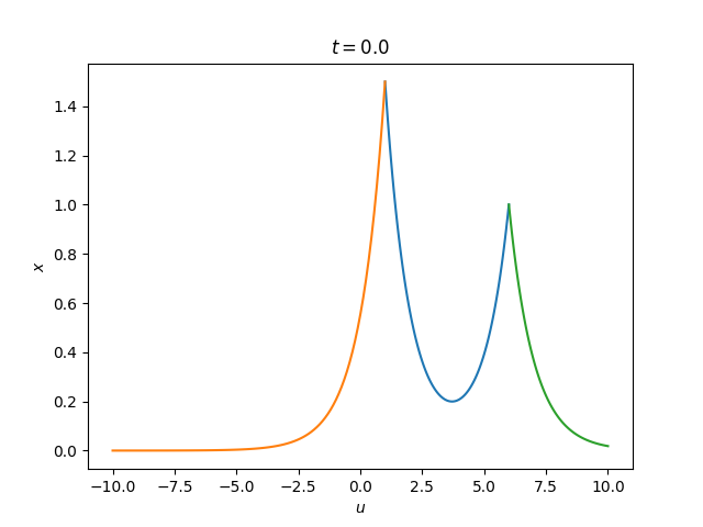
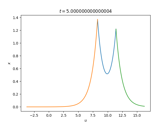
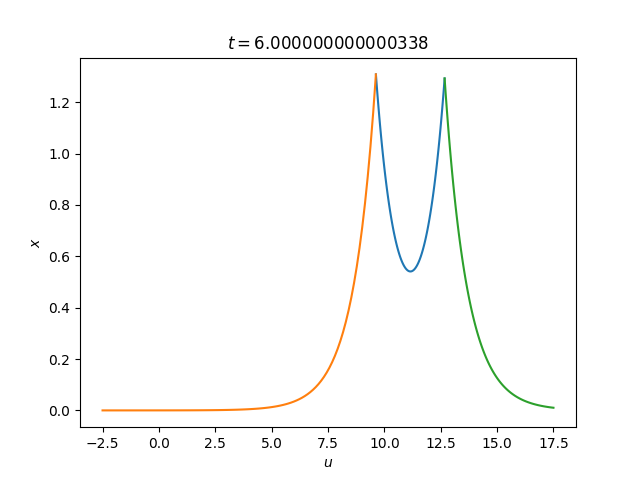
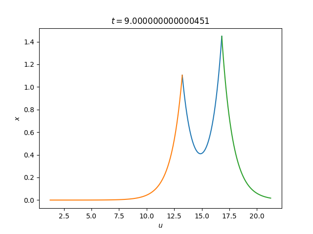
Figure 1. Plots of $u(x)$ from the overtaking collision for $r=2$ at various times. Top-left: $t=0$. Top-right: $t=3$. Bottom-left: $t=5$. Bottom-right: $t=9$. The peakon on the left has a higher velocity and so it catches up with the peakon on the right, transferring momentum through nonlocal interactions until the peakon on the right is moving faster and they separate again.

.

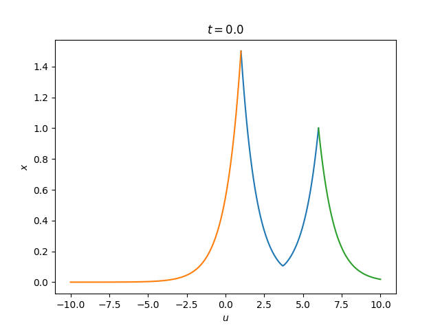
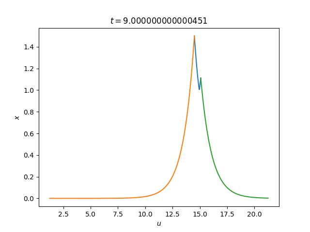
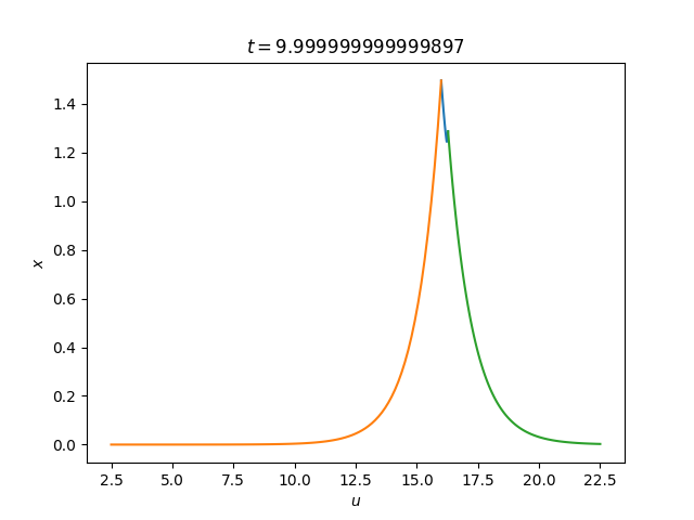
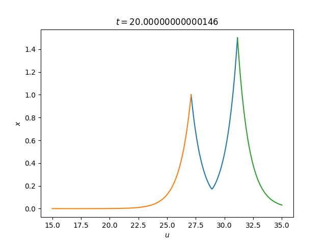
Figure 2. Plots of $u(x)$ from the overtaking collision for $r=6$ at various times. Top-left: $t=0$. Top-right: $t=9$. Bottom-left: $t=10$. Bottom-right: $t=20$. The main observable differences are that there is a much sharper minimum between the two peaks for $r=6$ than for $r=2$ in the previous figure, and the two peaks get much closer to each other during the collision for $r=6$ than for $r=2$.

.

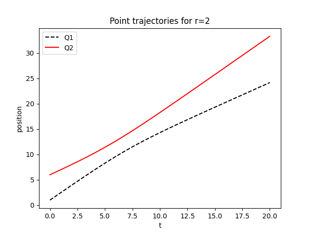
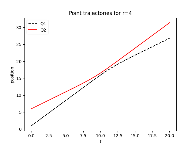
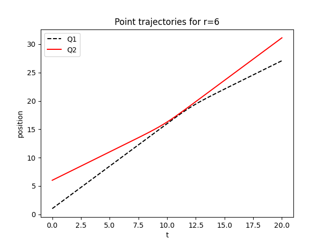
Figure 3. Plots of $Q_{1}$ and $Q_{2}$ versus time for various $r$: Top-left: $r=2$. Top-right: $r=4$. Bottom: $r=6$. For larger $r$, we see that the peaks are behaving much more like billiard balls, with the elastic interaction being much more local and therefore producing much less phase shift. This is because in the $\operatorname{W}^{1,r}$ norm, a smaller reduction in the larger peak is required to balance the same increase in the smaller peak.

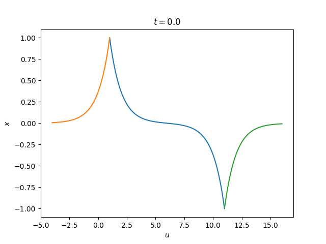
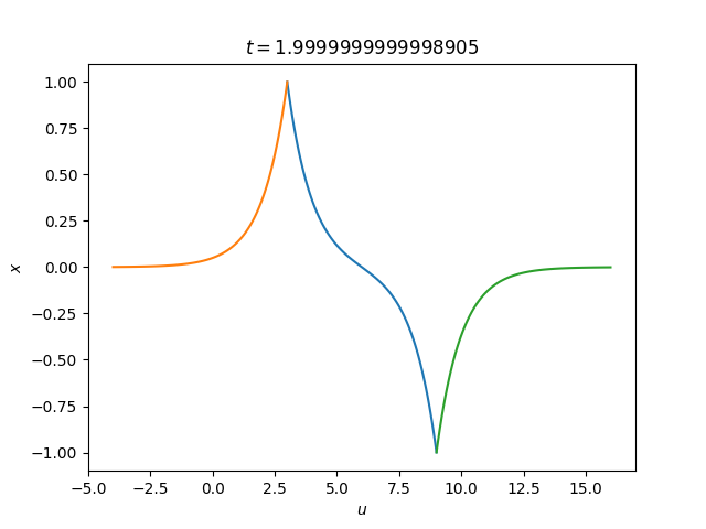
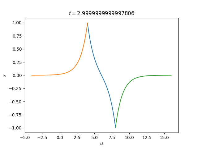
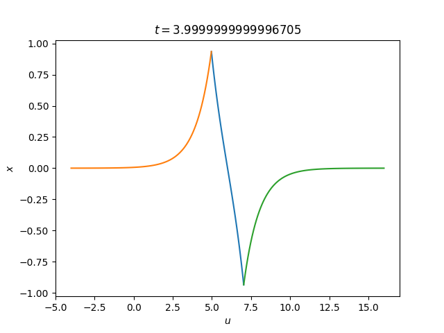
Figure 4. Plots of $u(x)$ from the antisymmetric collision for $r=2$ at various times. Top-left: $t=0$. Top-right: $t=2$. Bottom-left: $t=3$. Bottom-right: $t=4$. As the peaks get closer together, the profile between the peaks approaches a straight line, with the derivative becoming more and more negative. This causes $P_{1}$ and $P_{2}$ to get larger, preventing the two peaks from cancelling each other out and leading to a collision in finite time.

.

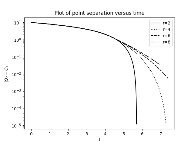
Figure 5. Antisymmetric collision paths for various values of $r$ ranging from from $r=2$ to $r=8$. We see that the collision takes the shortest time for $r=2$, and the collision time is increasing as $r$ increases from 2 to 8. This behaviour is consistent with the hypothesis that the collision time tends to infinity as $r\to\infty$.

5.2. 2 point solutions

Now we solve the $N=2$ case. It is necessary to use numerical methods to solve the equation for the singular solution profile in $[Q_{1},Q_{2}]$, either by solving the quadratures in Appendix A, or by using a direct numerical discretisation of (53). In this section we compute peakon solutions by solving (53) numerically in each interval $[Q_{i},Q_{i+1}]$, using a finite element discretisation, implemented using Firedrake (Rathgeber et al., 2016).

For two point solutions, the range $[Q_{1},Q_{2}]$ is transformed to the unit interval $[0,1]$, to facilitate symbolic differentiation to compute the Hamiltonian vector field. Then we can write

(78) $$L[u,Q]=\hat{L}[\hat{u},Q]=\frac{1}{r}\Delta Q\int_{0}^{1}\hat{u}^{r}+\frac{1}{(r-1)\Delta Q^{r}}\hat{u}_{s}^{r}\operatorname{d}s+\frac{1}{r(r-1)}(\hat{u}(0))^{r}+\frac{1}{r(r-1)}(\hat{u}(1))^{r},$$

where $\Delta Q=Q_{2}-Q_{1}$, and $u(Q_{1}+s\Delta Q)=\hat{u}(s)$, having made use of the identities,

(79) $$u(x)=\left\{\begin{array}[]{cc}\hat{u}(1)e^{Q_{2}-x}&x>Q_{2}\\ \hat{u}(0)e^{x-Q_{1}}&x<Q_{1}\\ \end{array}\right.,$$

which leads to

(80) $$\frac{1}{r}\int_{Q_{N}}^{\infty}u^{r}+\frac{u_{x}^{r}}{r-1}\operatorname{d}x =\underbrace{\frac{1+\frac{1}{r-1}}{r}}_{=\frac{1}{r-1}}\hat{u}(1)^{r}\int_{Q_{N}}^{\infty}e^{r(Q_{N}-x)}\operatorname{d}x,$$

(81) $$=-\frac{1}{r(r-1)}(\hat{u}(1))^{r}[e^{r(Q_{N}-x)}]_{Q_{N}}^{\infty}=\frac{1}{r(r-1)}(\hat{u}(1))^{r},$$

and

(82) $$\frac{1}{r}\int_{-\infty}^{Q_{1}}u^{r}+\frac{u_{x}^{r}}{r-1}\operatorname{d}x =\underbrace{\frac{1+\frac{1}{r-1}}{r}}_{=\frac{1}{r-1}}(\hat{u}(0))^{r}\int_{-\infty}^{Q_{1}}e^{r(x-Q_{1})}\operatorname{d}x,$$

(83) $$=\frac{1}{r(r-1)}(\hat{u}(0))^{r}[e^{r(x-Q_{1})}]_{Q_{1}}^{\infty}=\frac{1}{r(r-1)}(\hat{u}(0))^{r}.$$

The Hamiltonian is then $H(P,Q)=S(\tilde{u},P,Q)$, where

(84) $$S[P,Q,\tilde{u}]=P_{1}\tilde{u}(0)+P_{2}\tilde{u}(1)+\hat{L}[\tilde{u},Q],$$

and where $\tilde{u}$ is constrained to solve

(85) $$\left\langle\frac{\delta S}{\delta\tilde{u}},\delta\tilde{u}\right\rangle=0,\quad\forall\delta\tilde{u}\in V.$$

For the unapproximated problem $V=\operatorname{W}^{1,r}([0,1])$, which we approximate with a conforming finite element space $V_{h}\subset V$. We have

(86) $$\frac{\partial H}{\partial Q_{i}}=\frac{\partial S}{\partial Q_{i}}+\underbrace{\left\langle\frac{\partial S}{\partial\tilde{u}},\frac{\partial\tilde{u}}{\partial Q_{i}}\right\rangle}_{=0},\quad i=1,2,$$

provided that (85) is satisfied. Similarly we have $\frac{\partial H}{\partial P_{i}}=\frac{\partial S}{\partial P_{i}}$, $i=1,2$. Hence, the Hamiltonian equations are

(87) $$\left\langle\frac{\partial S}{\partial\tilde{u}},v\right\rangle=0,\forall v\in V_{h},\,\accentset{\mbox{\large.}}{P}_{i}=-\frac{\partial S}{\partial Q_{i}},\,\accentset{\mbox{\large.}}{Q}_{i}=\frac{\partial S}{\partial P_{i}},$$

all of which can be obtained by symbolic differentation using Firedrake.

First we consider the “overtaking” collision, where $Q_{1}=1$, $Q_{2}=6$, $u(Q_{1})=1.5$, and $u(Q_{2})=1$ initially. Some plots are showing in Figure 1 and Figure 2, for $r=2$ and $r=6$ respectively. We observe that for larger $r$, the peaks behave more like billiards, with the collision being more local (i.e., the peaks get closer before transferring momentum from the peak on the left to the peak on the right). This is made clearer in Figure 3, which shows the peak trajectories for $r=2,4,6$. The same momentum transfer occurs in each case, but the peaks get closer before transferring for larger $r$. This is because for larger $r$, a smaller reduction in the larger peak is required to balance the same increase in the smaller peak in order to preserve the $\operatorname{W}^{1,r}$ norm.

Next we consider the “antisymmetric” collision, where $Q_{1}=1$, $Q_{2}=11$, $u(Q_{1})=1$, and $u(Q_{2})=-1$ initially. The classic collision is seen in Figure 4. If the peaks were simply superposed, they would cancel out, but the nonlinear interaction drives up $P_{1}$ (and $P_{2}$ towards $-\infty$), keeping $u(Q_{1})>0>u(Q_{2})$, leading to a collision in finite time. Now we examine how this finite time collision behaves for different $r$ in Figure 5. We see a trend in increasing collision time as $r$ increases from 4 to 10. This is consistent with the hypothesis that the collision time should tend to infinity as $r\to\infty$. Similar results for the r-Hunter-Saxton equation were observed in Cotter et al. (2020).

5.3. 3 point solutions

We finally present a three point solution, with $r=4$, obtained using the 3 point extension of the same finite element method used to produce the 2 point solutions. The initial condition is chosen so that all three points are moving in the same direction, but the point farthest to the left is moving at faster speed than the two points on the right. Plots of the solution at various times are given in Figures 6 and 7. It appears that the three points have clumped together (as we see at $t=25$ in Figure 6). However, in Figure 7, we see that the points separate again at later times. A plot of the trajectories is shown in Figure 8. This plot shows that the ordering of the points is preserved, as we expect from the fact that the points are transported by a globally defined velocity $u$ (i.e. they are acted on by the time-dependent diffeomorphism generated by $u$). One may notice that when the points are almost superposed, the peak is only slightly higher than the left peak in the initial condition. This is due to the 4th power in the energy as opposed to the 2nd power for CH.

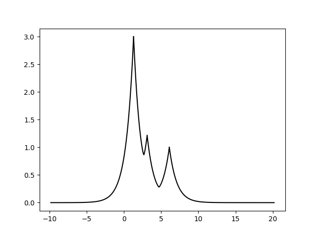
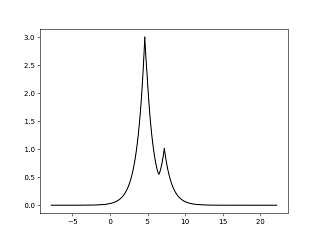
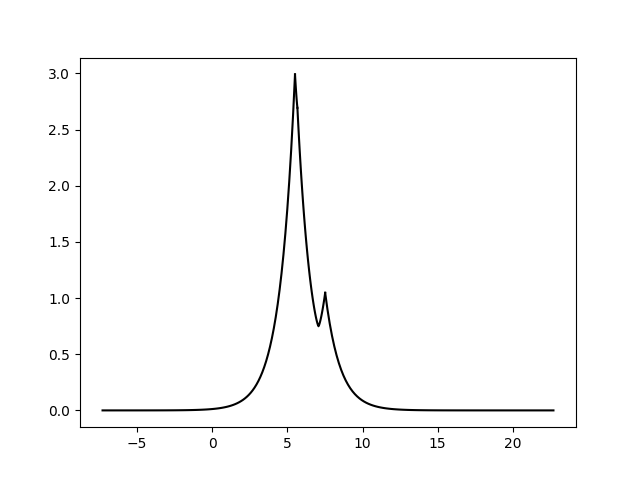
Figure 6. Plots of the three point solution with initial condition $Q_{1}=1$, $Q_{2}=3$, $Q_{3}=6$, $u_{1}=3$, $u_{2}=1.2$, $u_{3}=1$. From left to right, then top to bottom, the solution is plotted at times $t=1,12,15$ and 25 respectively. Plots at later times are shown in Figure 7.

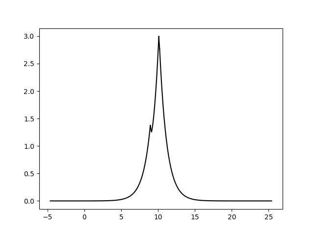
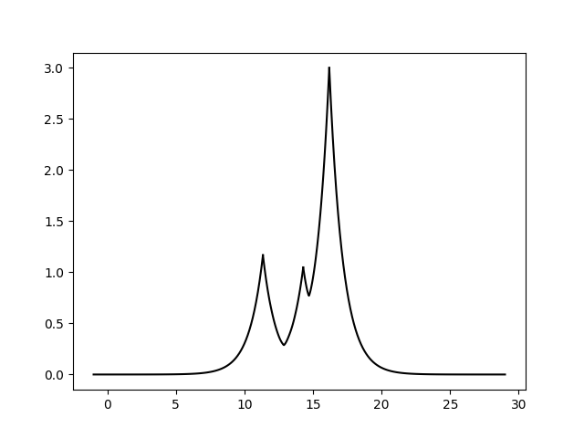
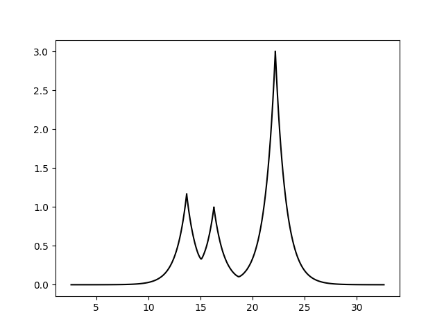
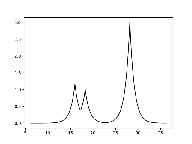
Figure 7. Plots of the three point solution with initial condition $Q_{1}=1$, $Q_{2}=3$, $Q_{3}=6$, $u_{1}=3$, $u_{2}=1.2$, $u_{3}=1$. From left to right, then top to bottom, the solution is plotted at times $t=30,50,70$ and 90 respectively. Earlier times are plotted in Figure 6. Eventually the gap will widen between the two points on the left.

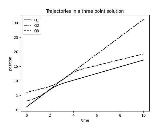
Figure 8. Point trajectories of the three point solution with initial condition $Q_{1}=1$, $Q_{2}=3$, $Q_{3}=6$, $u_{1}=3$, $u_{2}=1.2$, $u_{3}=1$. We observe that the points pass very close to each other but do not cross, so their order does not change.

6. Summary and outlook

Our main goal in this paper has been to demonstrate the existence of singular weak solutions of the r-CH equation and numerically simulate the coherence of their nonlinear interactions in overtaking collisions and head-on collisions. Of course, many questions remain open about the r-CH solutions. For example, we have not studied their stability, or even the stability of their $N=1$ travelling wave. However, the numerical simulations indicate that these solutions are likely to be quite stable. The outcome of their head-on collisions raises some questions, though, since wave breaking (that is, the formation of a vertical derivative of velocity) was not seen in the simulations for $r>2$. The absence of wave breaking raises the question of whether these singular weak solutions would emerge from smooth initial conditions in finite time. However, wave breaking may not be relevant to the formation of the $N$-point solutions. In fact, wave breaking may not be relevant to the creation of CH peakons for $r=2$, either. See (Bendall et al. (2021)) for a discussion of other mechanisms of creation of CH peakons. We plan to investigate the emergence of singular solutions from smooth initial conditions by solving Equation (26) using a finite element method in future work. The present work also ignores any analytical questions of local well-posedness (existence, uniqueness and continuous dependence on initial conditions) for the r-CH solutions arising from smooth initial conditions. Finally, it is interesting to ask how the singular solutions produce solutions of the integrated equation (26) even though they are insufficiently regular to solve the r-CH equation that emerges from Hamilton’s principle. We hypothesise that this is because the singular solutions are solutions to the optimal control problem

(88) $$\min_{u,Q}\int_{0}^{T}\|u\|_{\operatorname{W}^{1,r}}\operatorname{d}t,$$

subject to the constraints

(89) $$\accentset{\mbox{\large.}}{Q}_{i}=u(Q_{i},t),\quad Q_{i}(0)=a_{i},\,Q_{(}T)=b_{i},\quad i=1,\ldots,N.$$

We could then find a minimising sequence of smooth solutions of the r-CH equation that satisfy these constraints, recovering the singular solutions in the limit. Since the limit only ensures a solution in $\operatorname{W}^{1,r}$, we would lose the property of solving the r-CH equation, but solving the integrated equation (26) is still possible (since all of the smooth solutions also solve it). All these questions and crowds of other related questions that may come easily to mind will be left open for future work.

Acknowledgements

We would like to thank our friends and colleagues who have generously offered their attention, thoughts and encouragement in the course of this work during the time of COVID-19. We thank Jonathan Mestel for useful discussions about Equation (53), which kickstarted this work. CJC is grateful for partial support from EPSRC (EP/W015439/1, EP/W016125/1, EP/R029423/1, EP/R029628/1, EP/L016613/1) and NERC (NE/R008795/1). DH is grateful for partial support from ERC Synergy Grant 856408 - STUOD (Stochastic Transport in Upper Ocean Dynamics). TP is grateful for partial support from EPSRC (EP/X017206/1, EP/X030067/1 and EP/W026899/1) and the Leverhulme Trust (RPG-2021-238).

Appendix A Solving for the characteristic constants $C_{i}$

The sign of $C_{i}$ determines the characteristic behaviour of the solution. If $C_{i}>0$, then $u$ cannot have a zero. Conversely, for $C_{i}<0$, $u$ cannot have a turning point. We call these two situations the “cosh-like” and “sinh-like” solutions, respectively. When $C_{i}=0$, we have exponential solutions $u(x)=a\exp(\pm x)$, with the constant $a$ and the sign is to be determined from the boundary conditions: when $x<Q_{1}$ we have $C_{i}=0$ and we take the positive sign. Conversely, we take the negative sign for $x>Q_{N}$.

To determine $C_{i}$ for $Q_{i}<x<Q_{i+1}$, $0<i<N$, given boundary values $\widehat{u}_{i},\widehat{u}_{i+1}$, we first determine the sign of $C_{i}$. If $\widehat{u}_{i}\times\widehat{u}_{i+1}<0$, then by continuity there must be a root, and so $C_{i}<0$. If $\widehat{u}_{i}\times\widehat{u}_{i+1}\geq 0$, we first eliminate the case $C_{i}=0$ by fitting the exponential solution with positive sign if $\widehat{u}_{i+1}>\widehat{u}_{i}$ and negative sign otherwise. If the fit is successful, we have determined $C_{i}=0$. If it isn’t, then either the growth/decay is insufficiently large, and we have a sinh-like solution with $C_{i}<0$; or, otherwise, and we have a cosh-like solution with $C_{i}>0$.

If $C_{i}<0$, we determine the sign of $u_{x}$ from $\operatorname{sgn}(\widehat{u}_{i+1}-\widehat{u}_{i})=\sigma_{i}$. Then, we integrate (56) to get

(90) $$\operatorname{sgn}(\widehat{u}_{i+1}-\widehat{u}_{i})\int_{\widehat{u}_{i}}^{u(x)}\frac{\operatorname{d}w}{(w^{r}-C_{i})^{1/r}}=x-Q_{i}.$$

This implicit equation determines $u(x)$ given $x$, $C_{i}$, etc. We can compute the integral using numerical quadrature.

In particular, we have

(91) $$\operatorname{sgn}(\widehat{u}_{i+1}-\widehat{u}_{i})\int_{\widehat{u}_{i}}^{\widehat{u}_{i+1}}\frac{dw}{(w^{r}-C_{i})^{1/r}}=Q_{i+1}-Q_{i}.$$

This implicit equation relates $C_{i}$, $Q_{i}$, $Q_{i+1}$, $\widehat{u}_{i}$ when $C_{i}<0$.

If $C_{i}>0$, we have a turning point when $u^{r}(x^{*})=\pm C_{i}^{1/r}$. There is only one turning point, because $u$ has no root, and two turning points would imply a root. If $x^{*}\in[Q_{i},Q_{i+1}]$, then the sign of $u_{X}$ changes at the turning point. If $u_{i}$ and $u_{i+1}$ are both positive (they need to have the same sign, otherwise there is a root and $C_{i}$ must be negative), then $u_{x}$ must be negative for $x\in(Q_{i},x^{*})$ and positive for $x\in(x^{*},Q_{i+1})$. The signs are reversed when $u_{i}$ and $u_{i+1}$ are both negative.

Then, we have

(92) $$-\operatorname{sgn}(\widehat{u}_{i})\int_{\widehat{u}_{i}}^{C_{i}^{1/r}}\frac{\operatorname{d}w}{(u^{r}-C_{i})^{1/r}}+\operatorname{sgn}(\widehat{u}_{i})\int_{C_{i}^{1/r}}^{\widehat{u}_{i+1}}\frac{\operatorname{d}w}{(u^{r}-C_{i})^{1/r}}=Q_{i+1}-Q_{i}.$$

When computing the integrals by numerical quadrature, it is necessary to remove the weak singularity by a change of variables $v^{r}=w^{r}-C_{i}$, leading to, e.g.

(93) $$\int_{u_{1}}^{C_{i}^{1/2}}\frac{\operatorname{d}w}{(w^{r}-C_{i})^{1/r}}=\int_{(u_{1}^{r}-C_{i})^{1/r}}^{0}\frac{v^{r-2}\operatorname{d}v}{(v^{r}+C_{i})^{\frac{r-1}{r}}},$$

for which the integrand would have no singularity at $w^{r}=C_{i}$. If $x^{*}$ is outside the interval $\Omega_{i}$ (signalled by equation (92) having no solution), then $u_{x}$ has the same sign throughout the interval, as determined by the difference $\widehat{u}_{i+1}-\widehat{u}_{i}$, and we are back to the situation in (91).

References

- Barnes and Hone (2022) Barnes, L.E., Hone, A.N., 2022. Similarity reductions of peakon equations: the-family. Theoretical and Mathematical Physics 212, 1149–1167.
- Bauer and Maor (2021) Bauer, M., Maor, C., 2021. Can we run to infinity? The diameter of the diffeomorphism group with respect to right-invariant Sobolev metrics. Calculus of Variations and Partial Differential Equations 60, 1–35.
- Bendall et al. (2021) Bendall, T.M., Cotter, C.J., Holm, D.D., 2021. Perspectives on the formation of peakons in the stochastic Camassa–Holm equation. Proceedings of the Royal Society A 477, 20210224.
- Camassa and Holm (1993) Camassa, R., Holm, D.D., 1993. An integrable shallow water equation with peaked solitons. Physical Review Letters 71, 1661.
- Cotter et al. (2020) Cotter, C.J., Deasy, J., Pryer, T., 2020. The r-Hunter–Saxton equation, smooth and singular solutions and their approximation. Nonlinearity 33, 7016.
- Dimas and Tsoubelis (2004) Dimas, S., Tsoubelis, D., 2004. Sym: A new symmetry-finding package for mathematica. Proceedings of the 10th international conference in modern group analysis , 64–70.
- Dimas and Tsoubelis (2006) Dimas, S., Tsoubelis, D., 2006. A new mathematica-based program for solving overdetermined systems of pdes, in: 8th International Mathematica Symposium.
- Gay-Balmaz and Vizman (2012) Gay-Balmaz, F., Vizman, C., 2012. Dual pairs in fluid dynamics. Annals of Global Analysis and Geometry 41, 1–24.
- Holm and Marsden (2005) Holm, D.D., Marsden, J.E., 2005. Momentum maps and measure-valued solutions (peakons, filaments, and sheets) for the EPDiff equation, in: The breadth of symplectic and Poisson geometry. Springer, pp. 203–235.
- Holm et al. (1998) Holm, D.D., Marsden, J.E., Ratiu, T.S., 1998. The Euler–Poincaré equations and semidirect products with applications to continuum theories. Advances in Mathematics 137, 1–81.
- Kouranbaeva (1999) Kouranbaeva, S., 1999. The Camassa–Holm equation as a geodesic flow on the diffeomorphism group. Journal of Mathematical Physics 40, 857–868.
- Olver (1993) Olver, P.J., 1993. Applications of Lie groups to differential equations. volume 107 of Graduate Texts in Mathematics. Second ed., Springer-Verlag, New York.
- Papamikos and Pryer (2019) Papamikos, G., Pryer, T., 2019. A Lie symmetry analysis and explicit solutions of the two-dimensional -Polylaplacian. Studies in Applied Mathematics 142, 48–64.
- Rathgeber et al. (2016) Rathgeber, F., Ham, D.A., Mitchell, L., Lange, M., Luporini, F., McRae, A.T., Bercea, G.T., Markall, G.R., Kelly, P.H., 2016. Firedrake: automating the finite element method by composing abstractions. ACM Transactions on Mathematical Software (TOMS) 43, 1–27.
- Younes (2010) Younes, L., 2010. Shapes and Diffeomorphisms. volume 171. Springer.