ALMA detections of [O III] and [C II] emission lines from A1689-zD1 at $z=7.13$

Abstract

A1689-zD1 is one of the most distant galaxies, discovered with the aid of gravitational lensing, providing us with an important opportunity to study galaxy formation in the very early Universe. In this study, we report the detection of [C II]158 $\mu$m and [O III]88 $\mu$m emission lines of A1689-zD1 in the ALMA Bands 6 and 8. We measure the redshift of this galaxy as $z_{\rm{sys}}=7.133\pm 0.005$ based on the [C II] and [O III] emission lines, consistent with that adopted by Bakx et al. (2021). The observed $L_{[\rm{O\,III]}}/L_{[\rm{C\,II]}}$ ratio is $2.09\pm 0.09$, higher than most of the local galaxies, but consistent with other $z\sim 7$ galaxies. The moderate-spatial resolution of ALMA data provided us with a precious opportunity to investigate spatial variation of $L_{[\rm{O\,III]}}/L_{[\rm{C\,II]}}$. In contrast to the average value of 2.09, we find a much higher $L_{[\rm{O\,III]}}/L_{[\rm{C\,II]}}$ of $\sim 7$ at the center of the galaxy. This spatial variation of $L_{[\rm{O\,III]}}/L_{[\rm{C\,II]}}$ was seldom reported for other high-z galaxies. It is also interesting that the peak of the ratio does not overlap with optical peaks. Possible physical reasons include a central AGN, shock heating from merging, and starburst. Our moderate-spatial resolution data also reveals that in addition to the observed two clumps shown in previous HST images, there is a redshifted segment to the west of the northern optical clump. Such a structure is consistent with previous claims that A1689-zD1 is a merging galaxy, but with the northern redshifted part being some ejected materials, or that the northern redshifted materials being from a third more highly obscured region of the galaxy.

1 Introduction

Studies of high-redshift (high-$z$) galaxies are crucial in understanding the early phase of galaxy formation and evolution. A gravitationally-lensed galaxy A1689-zD1 is among the most distant sources ($z\sim$ 7.13) discovered so far, strongly lensed by a factor of $\mu=$9.3 (Bradley et al., 2008). It is, therefore, a useful probe to study the early Universe. Recently in Bakx et al. (2021), they adopted a new redshift of the galaxy $z=$7.13 , and our measurement confirms the redshift.

Having a high dust mass as compared to the Milky Way makes A1689-zD1 unusual among high-redshift dust emitters. It is also a sub-L* galaxy (Watson et al., 2015). The massive amount of dust may indicate a gas-rich system that makes the emission lines from interstellar medium (ISM) detectable. According to Bradley et al. (2008), A1689-zD1 is a system composed of two clumps, which are likely separate star-forming regions within the galaxy, but they could conceivably be interpreted as small star-forming galaxies merging at high redshift.

Previously, A1689-zD1 was detected in dust continuum with the Atacama Large Millimeter/submillimeter Array (ALMA) in the absence of emission lines (Knudsen et al., 2017; Bakx et al., 2021), except for a slight excess in [C II]158 $\mu$m (Knudsen et al., 2017). Using the dust continuum, the sizes of the two clumps detected were estimated to be $0.4-1.7$ kpc, and the dust temperature was approximated to be $T_{\rm{dust}}\sim 35-45$ K. A recent update of dust temperature and mass of A1689-zD1 using continuum estimated from [C II]-based method are $T_{\rm{dust}}=40^{+13}_{-7}$K and $M_{\rm{d}}=2.0^{+1.8}_{-1.0}\times 10^{7}$M_⊙ (Bakx et al., 2021).

In Watson et al. (2015), the redshift was measured from the X-shooter spectra taken on the Very Large Telescope (VLT), using the Ly$\alpha$ break due to the lack of Ly$\alpha$ and other emission lines. However, the redshift measurement based on the Ly$\alpha$ break is less certain than that using high excitation lines. Moreover, the break is close to the spectrograph’s near-infrared (NIR) / visual (VIS) arm split. Thus, the redshift needs to be measured more accurately. Using [C II] and [O III] emission lines, a redshift of 7.13 by spectral measurement adopted by Bakx et al. (2021) is confirmed in this work.

Since [O III]88 $\mu$m is bright for some galaxies at $z>6$ (e.g., Inoue et al., 2016; Carniani et al., 2017; Harikane et al., 2020), the [O III] line is one of the most useful tracers for ISM properties. In addition, [O III] has a higher ionization potential (35.1 eV) than [C II] (11.3 eV). Therefore, the [O III]/[C II] ratio is useful to investigate the ionization state.

In this paper, we present an analysis of archival ALMA data of [C II]158 $\mu$m and [O III]88 $\mu$m in Cycles 3 and 5 with a higher spatial resolution ($\sim$0^′′.2) than ever before ($\sim$0^′′.9 (Knudsen et al., 2017); 0^′′.6-0^′′.7 (Watson et al., 2015)). With this higher spatial resolution, the data can be used to examine the line emissions, resolve structures inside the galaxy, investigate velocity structures, etc., in comparison with the HST images. For example, this higher-spatial resolution allows us to examine the kinematic properties of A1689-zD1. We can also investigate the ratio of [O III]/[C II] as a function of positions within the galaxy. This is important because, as some previous studies discussed, the observed high [O III]/[C II] may be due to the difference in their spatial distributions (Carniani et al., 2017).

This paper is organized as follows. In section 2 we describe the ALMA dataset used in the study; section 3 presents the main results, with discussions in section 4. Finally, we present our conclusions in section 5. Throughout this paper, we assume the Planck15 cosmology (Planck Collaboration et al., 2016) as a fiducial model, i.e., a $\Lambda$ cold dark matter cosmology with ($\Omega_{m}$,$\Omega_{\Lambda}$,$\Omega_{b}$,$h$)=(0.308, 0.682, 0.0486, 0.678).

2 Observation

Two ALMA bands, Bands 6 and 8, are chosen in this study in order to characterize the physical properties of A1689-zD1. Because it is a dusty galaxy (Watson et al., 2015), it is important to measure the star-formation rate (SFR) derived from far-infrared (FIR) observations, using its relation with [C II]158 $\mu$m and [O III]88 $\mu$m emissions. At the redshift of A1689-zD1, Band 6 covers [C II], and Band 8 covers [O III] emission lines.

The Band 6 observation was carried out in 2016 from August 1 to August 25 (Cycle 3) with the ALMA 12m array, and an antenna configuration of C36-(4)/5 and C36-(5)/6 (project ID: 2015.1.01406.S, P.I.: D. Watson); while the Band 8 data was obtained from observations in 2018 from April to December (Cycle 5), also with 12m array, but an antenna configuration of C43-3 and C43-4 (project ID: 2017.1.00775.S, P.I.: D. Watson). The observational configurations are summarized in Table 1.

The calibration of visibility data from ALMA archive was conducted with the pipeline versions 4.7 and 5.4, for Band 6 and 8 respectively, provided by the ALMA project using the Common Astronomy Software Applications (CASA). For the Band 6 data targeting [C II], the channel width of the observation is 1.95 MHz. As for the Band 8 data targeting [O III], the channel width is 3.91 MHz. The total exposure time on source for Band 6 ([C II]) observation is 28,123 seconds $\sim$ 7.81 hours, while that for Band 8 ([O III]) observation is 12,337 seconds $\sim$ 3.43 hours. The maximum recoverable scale (MRS) for the Band 6 and Band 8 data are 5^′′.32 and 4^′′.58, which are larger than the detected signals as we discuss below.

Table 1: Observational configurations

	Band 6	Band 8
	[C II]158 $\mu$m	[O III]88 $\mu$m
Baseline lengths (m)	15 - 1605	15 - 784
Number of antennas	38 - 40	41 - 47
Spectral window 1 (GHz)	217.17 - 219.05	404.48 - 406.30
Spectral window 2 (GHz)	219.05 - 220.93	406.31 - 408.14
Spectral window 3 (GHz)	231.96 - 233.84	416.33 - 418.20
Spectral window 4 (GHz)	233.85 - 235.73	418.18 - 420.01
Channel width (MHz)	1.95	3.91
Exp. time on source (hour)	7.81	3.43
PWV (mm)	0.3 - 1.1	0.3 - 1.0
MRS (arcsec)	5.32	4.58

Note. — The PWV values for each of the band data are from separate measurement sets due to the long exposure time; therefore, we present the minimum and maximum of averages per Execution Block (EB).

Using the calibrated measurement set (MS), we create image cubes for [C II] and [O III] lines with a spectral resolution of 10 km s^-1. The beam size is controlled by the robustness parameter of the Briggs weighting and $uv$-tapering in the CASA task tclean(). First, we subtract the continuum in each band using the CASA task uvcontsub by selecting the frequency ranges without line detection, i.e., 232.000$\sim$233.420 GHz for Band 6; 416.342$\sim$416.823GHz and 417.588$\sim$418.178 GHz for Band 8. Next, in order to investigate both the morphology and photometry of A1689-zD1, we produce 2 sets of image cubes for each of the bands (Hashimoto et al., 2019b). Since we are interested in the extent of [C II] and [O III] emissions of the galaxy, we adopt a Briggs robust weighting of R$=$0.5, achieving a beam size of $0^{\prime\prime}.271\times 0^{\prime\prime}.243$ ($0^{\prime\prime}.387\times 0^{\prime\prime}.332$), with a position angle at $-$80^∘ ($-$89^∘) for Band 6 (8) data. As presented in section 3.1.1, the extended structure does not exceed the MRS in both bands. Hence, we use the image cube sets with Briggs robust parameter R$=$0.5 for morphology analysis of A1689-zD1. As for maximizing the sensitivity of collecting the flux as a point source, we use natural weighting by setting R$=$2, and further apply $uv$-tapering to 2^′′ so as to get the maximum flux of the extended source. The beam size is dramatically increased to $2^{\prime\prime}.640\times 2^{\prime\prime}.337$ ($1^{\prime\prime}.874\times 1^{\prime\prime}.790$) at $-$63^∘ ($-$70^∘) for Band 6 (8) data. This set of data is used for flux and related calculations of the galaxy. The characteristics of the calibrated images are summarized in Table 2.

Table 2: Summary of image characteristics

	Band 6	Band 6	Band 8	Band 8
	(Briggs)	(natural & $uv$-tapered)	(Briggs)	(natural & $uv$-tapered)
Beam major / minor axes (arcsec)	0.271 / 0.243	2.640 / 2.337	0.387 / 0.332	1.874 / 1.790
Beam position anglea (deg)	-80	-63	89	-70
Sensitivityb (mJy beam-1)	0.17	0.59	0.66	1.69

Note. — ^aThe beam PA is in degrees east of north by which the major axis is rotated. ^bSensitivity is defined as the RMS value of the cube image with 10 km s^-1 channel width.

3 Results

3.1 [C II] and [O III] emission lines

3.1.1 Spatial distribution

Using CASA task immoments, we obtain moment 0 maps of the Band 6 and Band 8 (Briggs) data by stacking the cube channels along the spectrum, covering $\sim$ 400 km s^-1 ($\sim$ 1.2 FWHM). It is to make sure the detections of emission lines are valid (Novak et al., 2019). This range of frequency is comparable to that in previous studies (Inoue et al., 2016; Matthee et al., 2017; Hashimoto et al., 2019a; Novak et al., 2019). Fig. 1 shows the [C II] (white contours) line emission at 3, 7, 11, and 15$\sigma$ levels, and [O III] (magenta contours) line emission at 3, 7, 11, 15, and 19$\sigma$ levels, overlaid on the combined Hubble Space Telescope (HST) color image. For the purpose of color display, we stack HST filters with F105W as blue color; F125W as green; and F160W as red (proposal ID: 11802, P.I.: Ford). There is a known coordinate offset between their ALMA image and HST image as an average value of 0${}^{\prime\prime}.4\sim 0^{\prime\prime}$.45 (Watson et al., 2015). We, thus, measure the position difference of the peaks between the ALMA Bands 6 and 8 data and the HST image we use, and shift the ALMA contours by 0^′′.386 along right ascension (RA) in order to match the peaks for a better comparison. Because the structures shown in Fig. 1 extend to a 3$\sigma$ detection that is within an area of $\sim 2^{\prime\prime}.3\times 1^{\prime\prime}.5$ for both [C II] and [O III], which is much smaller than the MRS of 5^′′.32 and 4^′′.58 for [C II] and [O III], respectively, we confirm that the structures observed are not artificial. Both [C II] and [O III] emission lines are spatially well resolved with angular resolutions of 0^′′.203 and 0^′′.232, respectively.

From the HST image shown in Fig. 1, we see that there are two clumps: one on the northeast (clump A), and one on the southwest (clump B). We refer them as clump A and clump B throughout the context.

Figure 1: [C II] (white) contours are drawn at 3, 7, 11, and 15 $\sigma$ levels ($\sigma_{\rm{[C\,II]}}\sim 17.1\,\rm{mJy\,beam^{-1}\,km\,s^{-1}}$), while [O III] (magenta) contours are drawn at 3, 7, 11, 15, and 19 $\sigma$ levels ($\sigma_{\rm{[O\,III]}}\sim 55.7\,\rm{mJy\,beam^{-1}\,km\,s^{-1}}$). Overlaid is a $\sim 3^{\prime\prime}.5\times 3^{\prime\prime}.5$ cutout image of HST data composed of images using the filters: F105W(blue), F125W(green), and F160W(red). The corresponding beam sizes of the Briggs Band 6 and Band 8 images used are $0^{\prime\prime}.271\times 0^{\prime\prime}.243$ at $-80^{\circ}$ and $0^{\prime\prime}.387\times 0^{\prime\prime}.332$ at $89^{\circ}$, respectively.

3.1.2 Spectra

Using elliptical apertures of 8^′′.5$\times$7^′′.5 and 6^′′.5$\times$5^′′.5 (both approximately 3 beams), we extracted spectra from the natural and $uv$-tapered Band 6 and Band 8 image cubes, respectively. The spectra are shown in blue in Fig. 2. This is to include all the flux obtainable by covering the area where the spatially extended emission may exist, for instance, the [C II]158 $\mu$m halos around $z\sim 6$ galaxies reported by Fujimoto et al. (2019). At around the rest frequencies of [C II]158 $\mu$m and [O III]88 $\mu$m, in Band 6 and Band 8 respectively, we detect a line emission with two peaks in each band, indicated as ‘redshifted’ and ‘blueshifted’ as shown in Fig. 2. They may indicate two merging components. More analyses are presented in sections 3.2 and 3.3. Here, we first fit the spectra with two Gaussians. We obtain two peaks of Gaussians centering at 233.58$\pm$0.05 GHz and 233.72$\pm$0.08 GHz, for [C II] using Band 6 data in panel (a). Similarly, for Band 8 data, we find two peaks of [O III] at 416.98$\pm$0.08 GHz and 417.23$\pm$0.11 GHz, respectively, after applying two-Gaussian fitting as shown in panel (b). The fitted results are shown as red dotted lines in Fig. 2. We acquire a redshift of $z_{\rm{[C\,II]red}}=7.137\pm 0.002$ for the redshifted part, and that of $z_{\rm{[C\,II]blue}}=7.132\pm 0.003$ for the blueshifted part, for [C II] line detections in Band 6. Accordingly, we obtain redshifts of $z_{\rm{[O\,III]red}}=7.137\pm 0.002$ and $z_{\rm{[O\,III]blue}}=7.132\pm 0.002$ with Band 8 [O III] detections, for the redshfited and blueshifted parts. We find that the redshifts we obtain from the [C II] and [O III] line detections are in good agreement with each other for both of the components.

The signal-to-noise ratio (S/N), defined as the ratio of the peak flux of the source (moment-0 map) to the background noise of the image, is calculated for both Band 6 and Band 8 (natural and $uv$-tapered) data, with a value of S/N = =51.5 for [C II] and S/N = 22.3 for [O III]. Note that for Briggs weighted data, the S/N values are calculated as 16.1 for [C II], and 27.9 for [O III].

Taking the average of the [O III] and [C II] redshifts, we obtain a systemic redshift $z_{\rm{sys}}=7.133\pm$0.005. This matches the adopted redshift $z=7.13$ in Bakx et al. (2021). The new redshift derived from FIR fine structure [C II] and [O III] lines, and hence is a better measurement than the previous estimate of $z\sim 7.5$ based on the Lyman break with no detection of any emission line (Watson et al., 2015).

Figure 2: Spectra of (a) [C II]158 $\mu$m and (b) [O III]88 $\mu$m using ALMA (a) Band 6 and (b) Band 8 data (natural & $uv$-tapered). The red dotted lines in each panel show the Gaussian fitting results of clumps A and B as indicated.

We measure the widths of the emission lines with their full widths at half maxima (FWHMs) in terms of velocity (km s^-1). Details of the measured and derived parameters, corrected with a lensing magnification factor of $\mu=$9.3 (Bradley et al., 2008), of the galaxy are summarized in Table 3. We also include 1$\sigma$ uncertainty of the parameters in Table 3. The emission-line fluxes of [C II] and [O III] are measured by integrating the flux density along velocity, obtaining a total of 548$\pm$56 mJy km s^-1 for [C II], and 640$\pm$69 mJy km s^-1 for [O III]. We note that each flux error mentioned above is calculated by a quadrature sum of (i) fitting error of the emission line and (ii) 10% error due to the uncertainty in the absolute flux scale of ALMA data. With total line fluxes and systemic redshift deduced, we derive the line luminosities with the equation:

$$L_{\rm line}=1.04\times 10^{-3}\times\left(\frac{S_{\rm line}\,\Delta v}{\rm Jy\,km\,s^{-1}}\right)\left(\frac{D_{\rm L}}{\rm Mpc}\right)^{2}\left(\frac{\nu_{\rm obs}}{\rm GHz}\right)\,L_{\odot}$$ (1)

(Weinberg, 1972; Solomon et al., 1992; Carilli & Walter, 2013), where $S_{\rm{line}}\Delta v$ is the measured flux of the line, $D_{\rm{L}}$ is the luminosity distance, and $\nu_{\rm{obs}}$ is the observed frequency. The total luminosity of [C II] obtained is (69.2$\pm$1.2)$\times$10⁷ $L_{\odot}$, and that of [O III] is (144.5$\pm$5.7)$\times$10⁷ $L_{\odot}$. The obtained $L_{\rm{[C\,II]}}$ is slightly different from the value of (6.1$\pm$0.7)$\times$10⁸ $L_{\odot}$ adopted by Bakx et al. (2021) by nearly 1$\sigma$. Possible reasons may include different integration regions, beam sizes of the images, the parameter settings of $uv$-tapering, and/or different frequency ranges included.

Table 3: Measured and derived parameters of A1689-zD1, with lensing magnification ($\mu=$9.3) corrected

	[C II]158 $\mu$m		[O III]88 $\mu$m
peak	redshifted	blueshifted	redshifted	blueshifted
Central frequency (GHz)	233.58 $\pm$ 0.05	233.72 $\pm$ 0.08	416.98 $\pm$ 0.08	417.23 $\pm$ 0.11
Redshift	7.137 $\pm$ 0.002	7.132 $\pm$ 0.003	7.137 $\pm$ 0.002	7.132 $\pm$ 0.002
Emission-line width (km s-1)	150 $\pm$ 20	237 $\pm$ 19	122 $\pm$ 21	211 $\pm$ 21
Total emission-line width (km s-1)	323 $\pm$ 8		311 $\pm$ 17
Emission-line flux (mJy km s-1)	124$\pm$13	423$\pm$43	165$\pm$18	475$\pm$53
Total line flux (mJy km s-1)	548 $\pm$ 56		640 $\pm$ 69
Luminosity ($10^{7}L_{\odot}$)	15.7$\pm$1.6	53.5$\pm$5.5	37.2$\pm$4.2	107.3$\pm$12.0
Total luminosity ($10^{7}L_{\odot}$)	69.2 $\pm$ 7.0		144.5 $\pm$ 15.5

Note. — ^∗All errors are shown in 1$\sigma$. ^∗∗“Emission-line width”, “Emission-line flux”, and “Luminosity” indicate those of separate components derived by the spectral fitting analysis, while “Total emission-line width”, “Total line flux”, and “Total luminosity” indicate those of the redshifted and blueshifted line emission as a whole. ^∗∗∗For the errors of fluxes and luminosities, other than the fitting errors that we obtain, we also include 10% errors in the quadratures due to the absolute calibration uncertainty of ALMA data.

3.2 [O III]/[C II] ratio and Luminosity

$L_{\rm{[C\,II]}}$ and $L_{\rm{[O\,III]}}$ are calculated using the derived redshift of $z=7.133\pm 0.005$, so that $L_{\rm{[C\,II]}}=(69.2\pm 1.2)\times 10^{7}L_{\odot}$ and $L_{\rm{[O\,III]}}=(144.5\pm 5.7)\times 10^{7}L_{\odot}$. We, thus, obtain a total [O III]-to-[C II] luminosity ratio of $2.09\pm 0.09$.

With the obtained $L_{\rm{[C\,II]}}$, we can also revise the $SFR$ of the system using the relation:

$$SFR_{\rm{[C\,II]}}=1.0\times 10^{-7}\left(\frac{L_{\rm{[C\,II]}}}{L_{\odot}}\right)^{0.98},$$ (2)

in De Looze et al. (2011), which assumed a Kroupa Initial Mass Function (IMF) (Kroupa, 2001). We obtain a $SFR_{\rm{[C\,II],Krou}}=$ 46.1$\pm$0.8 M_⊙ $\rm{yr^{-1}}$. In Bakx et al. (2021), however, their dust-obscured SFR was derived from an IR luminosity-to-SFR relation which assumes a Salpeter IMF, with an estimated value of $SFR_{\rm{obsc,Sal}}=$ 33$\pm$9  M${}_{\odot}\,$yr^-1. In order to compare the SFR value we obtain with that derived in Bakx et al. (2021), we divide our SFR value by a factor of 0.67 to convert it to a Salpeter IMF based SFR (Madau & Dickinson, 2014); thus, it becomes $SFR_{\rm{[C\,II],Sal}}=$ 68.8$\pm$1.2 M_⊙ $\rm{yr^{-1}}$. This value is about 2 times the value derived by Bakx et al. (2021). The exact reason for the difference is not clear. Possible reasons include: (1) that the relation from De Looze et al. (2011) was derived from photometric data corrected for attenuation, while Bakx et al. (2021) derived the SFR from SED fitting result; (2) temperature dependence of [C II]-SFR relation (Malhotra et al., 1997); and/or (3) uncertainty in the SED fitting due to limited FIR photometric coverage. Additional further FIR data points would improve the SED fitting. Despite the difference, according to the bottom panel of Fig. 4 in De Looze et al. (2011), the logarithmic difference between the SFR derived from attenuation and that from [C II] line is still within a reasonable range. De Looze et al. (2011) presented almost an order of scatter on the SFR-[C II] relation, along with detailed discussions.

We show the [O III]/[C II] luminosity ratio map overlaid by black contours of [C II] emission-line flux at 3, 7, 11 and 15$\sigma$ levels, and magenta contours of [O III], emission-line flux at 3, 7, 11, 15 and 19$\sigma$ levels in Fig. 3.

In order to make a comparison between the two emissions, we need to enlarge the beam size of Band 6 [C II] data to that of Band 8 [O III] data before taking the ratio. Therefore, we apply a $uv$-tapering in the CASA task tclean() to the [C II] Briggs image to reach a spatial resolution that roughly matches that of the [O III] Briggs image, and further match the synthesized beam size and position angle of the [O III] cube exactly with the tclean() parameter restoringbeam. After matching the beam size of [C II] data to that of [O III] data, we use a python package reproject to reproject the finer pixel size of [C II] data from from (0^′′.035/pix $\times$ 0^′′.035/pix) to (0^′′.060/pix $\times$ 0^′′.060/pix), in order to match that of [O III] data (0^′′.060/pix $\times$ 0^′′.060/pix). Then, we divided the two arrays and re-created the [O III]/[C II] ratio map.

This is one of the rare cases that a spatial distribution of [O III]/[C II] map is revealed at $z>$7. Interestingly, [O III]/[C II] ratio is the highest around the center of the galaxy with a value of $\sim$7, and gradually decreases toward the outer parts of the galaxy, reaching a ratio of one. We further discuss the implications in section 4.1.

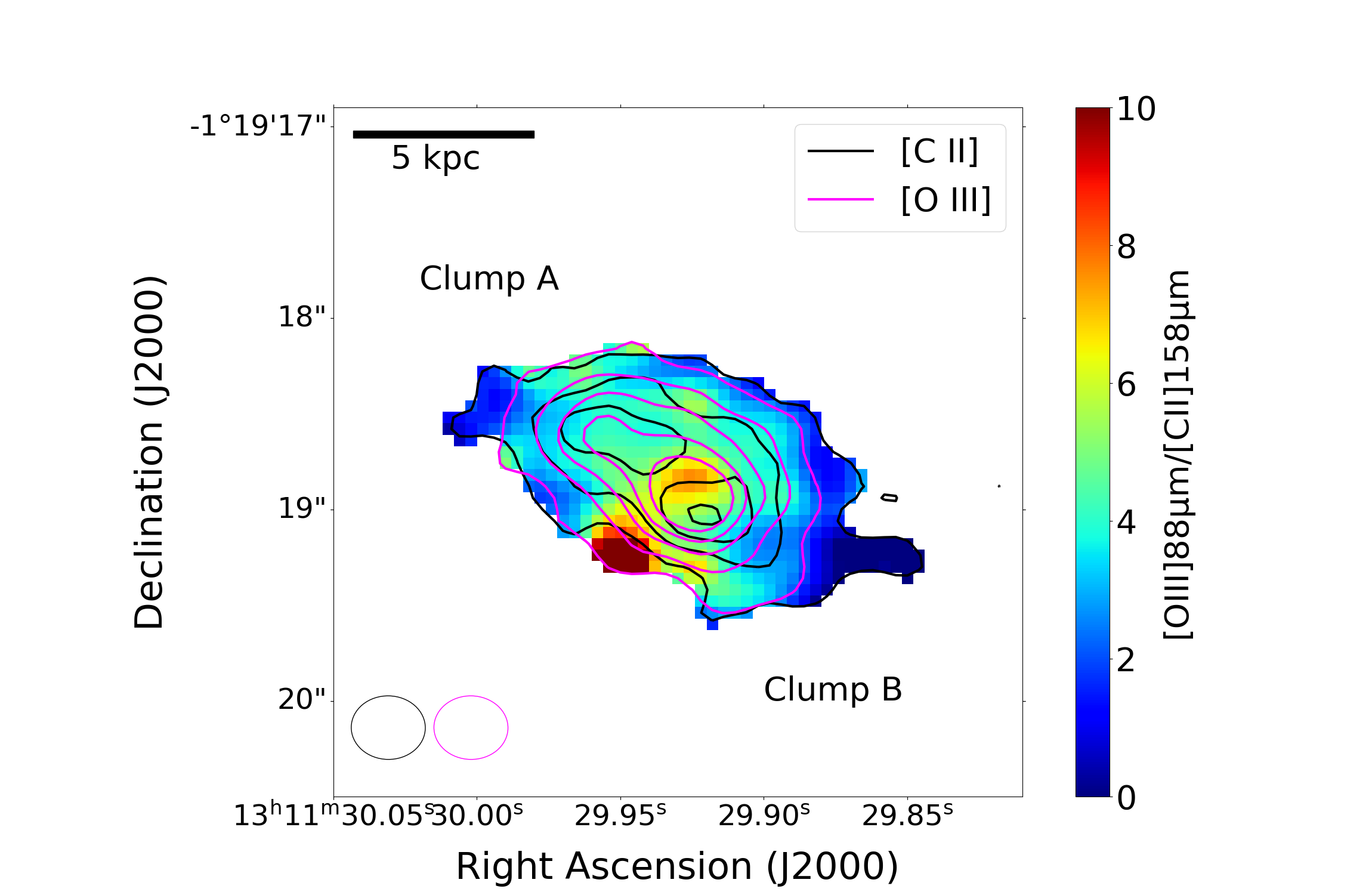
Figure 3: The [O III]88$\mu$m-to-[C II]158$\mu$m ratio map. Black contours show [C II]88$\mu$m line emission, while magenta contours show [O III] emission. [C II] contours are shown at 3, 7, 11 and 15$\sigma$ levels, where $\sigma_{\rm{[C\,II]}}\sim$17.1 mJy beam^-1 km s^-1. [O III] contours are shown at 3, 7, 11, 15, 19$\sigma$ levels, where $\sigma_{\rm{[O\,III]}}\sim$55.7 mJy beam^-1 km s^-1. The color bar shows the value of [O III]-to-[C II] luminosity ratio. The smaller beam size ($0^{\prime\prime}.271\times 0^{\prime\prime}.243$) and finer pixel size (0^′′.035/pix $\times$ 0^′′.035/pix) of the corresponding Band 6 (Briggs) are enlarged to ($0^{\prime\prime}.387\times 0^{\prime\prime}.332$; 0^′′.060/pix $\times$ 0^′′.060/pix) to match those of Band 8 data (Briggs). The pixels with [C II] and [O III] fluxes lower than 3 $\sigma$ are masked out. The resulting beam sizes are shown on the lower left of the figure.

In Fig. 4, we show the [O III]/[C II] luminosity ratio as a function of the bolometric luminosity, which is defined as the summation of the UV and total infrared (TIR) luminosities, i.e., $L_{\rm{bol}}=L_{\rm{UV}}+L_{\rm{TIR}}$ (Hashimoto et al., 2019b; Harikane et al., 2020). For comparisons, we also plot the ratios for $z=6$–9 galaxies in the literature plotted in Carniani et al. (2020) before applying Surface Brightness Dimming (SBD), as well as those of local galaxies studied in the Dwarf Galaxy Survey (Madden et al., 2013; De Looze et al., 2014; Cormier et al., 2015) and the Great Observatories All-sky LIRG Survey (GOALS: Howell et al., 2010; Díaz-Santos et al., 2017). The orange line is the fitting function of $z=6$-9 galaxies without A1689-zD1, adopted from Equation (7) in Harikane et al. (2020), as a comparison. Although as suggested in Carniani et al. (2020), SBD may affect the flux measurements gravely with ALMA, we do not apply the same correction because of the high S/N ratio of [C II] emission of A1689-zD1 ($\sim$17.1). Such an effect was predicted to be weak at high S/N ratio (Carniani et al., 2020). We find that A1689-zD1 and other $z=6$–9 galaxies show systematically higher [O III]/[C II] ratios than most of the local galaxies, which is consistent with previous results (Inoue et al., 2016; Laporte et al., 2019).

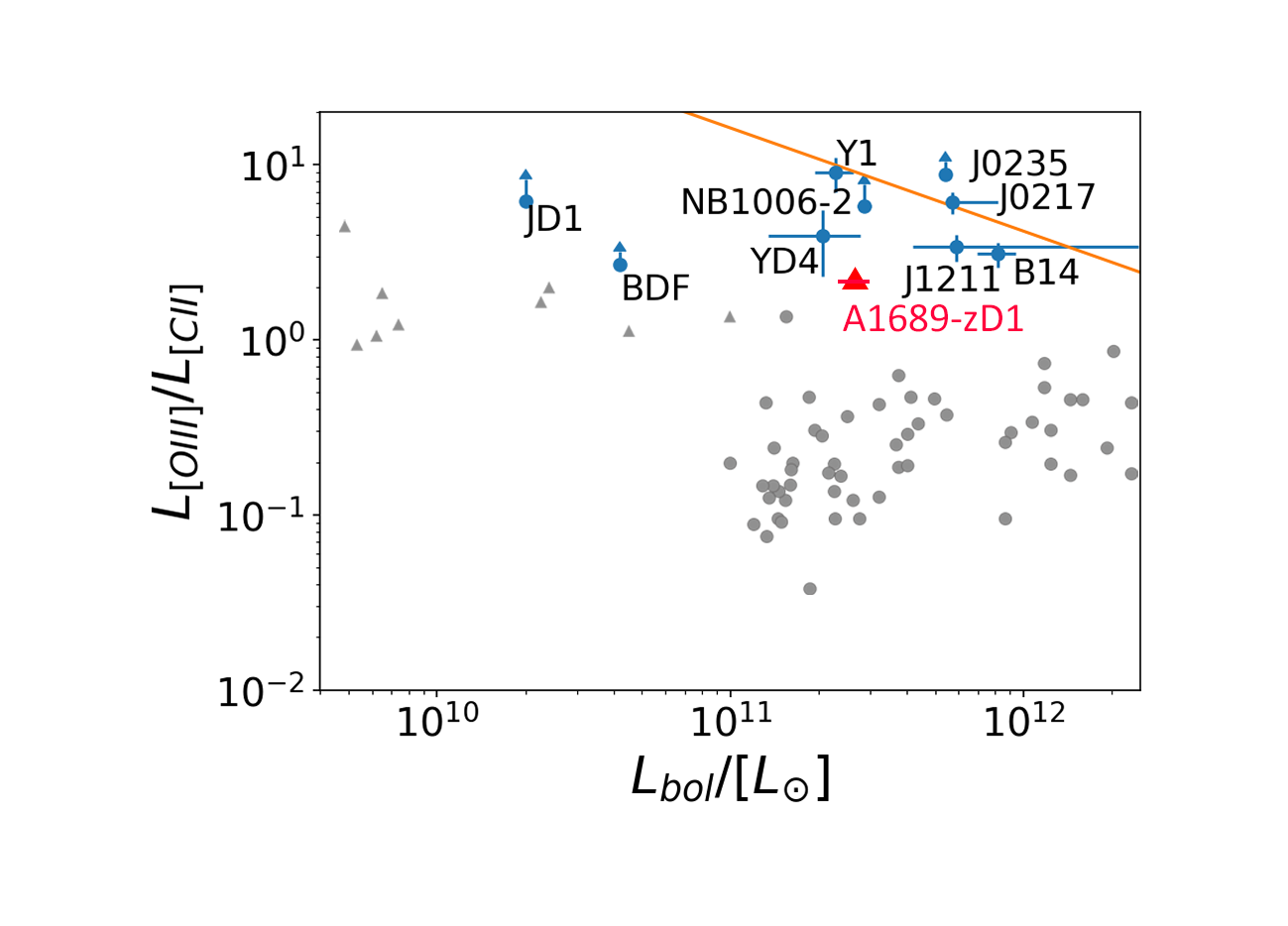
Figure 4: [O III]88$\mu$m/[C II]158$\mu$m luminosity ratio as a function of bolometric luminosity. The red triangle shows the data point for A1689-zD1. The bolometric luminosities of $z=6-9$ galaxies are taken from Hashimoto et al. (2019b), while the orange line is adopted from Equation (7) in Harikane et al. (2020), which is the fitting function of $z=6-9$ galaxies.The gray triangle and circles denote $z\sim$0 galaxies from the Dwarf Galaxy Survey (Madden et al., 2013; De Looze et al., 2014; Cormier et al., 2015) and Great Observatories All-sky LIRG Survey (GOALS: Howell et al., 2010; Díaz-Santos et al., 2017), respectively. The bolometric luminosity is estimated as a total of UV and TIR luminosities.

3.3 Velocity fields

In this section, we investigate the kinematic properties of A1689-zD1 using [O III] and [C II] emissions. With the CASA task immoments, we create flux-weighted velocity (i.e., moment 1) maps of [C II] and [O III] emission lines (Fig. 5), using pixels with $>$2$\sigma$ detections of Briggs data. Note that we do not consider the beam smearing effect for the velocity fields.

Comparing the clumps A and B we observe in Fig. 1, we see that clump A is consisted of a blueshifted component on the upper left (east side) and a redshifted component on the upper right (west side), while clump B is a cloud of redshifted and blueshifted mixture, but not as intense as the components in clump A.

We only investigate the [C II] field because: (1) Band 6 data ([C II]) has a better S/N compared to Band 8 data ([O III]), and (2) the patterns and the values of velocity field in [C II] and [O III] are similar.

A1689-zD1 might be a merger due to the parallel isovelocity lines found between clump A and clump B, as how it has been claimed (Bradley et al., 2008; Knudsen et al., 2017). A comparison to Fig. 1 shows that the two peaks of [C II] are consistent with clump B and the blueshifted part of clump A, while the redshifted part of clump A could possibly be (1) some ejected materials from the merger, or (2) from a highly obscured component of the galaxy. Similar discussions can be found in Jones et al. (2017) and Hashimoto et al. (2019b), while further comparisons to other targets are presented in section 4.2.

Figure 5: The velocity field (moment 1 map) of the emission lines (top: [C II]158$\mu$m and bottom: [O III]88$\mu$m; using Briggs weighted data). The gray contour in the top (bottom) panel is the same as the white (magenta) contour for [C II] ([O III]) emission in Figure. 1. Color bar in each panel shows the velocity in the range of -225 km s${}^{-1}\sim$135 km s^-1, as it is close to and covers the maximum and minimum values of both emissions.

4 Discussion

4.1 High [O III]/[C II] luminosity ratio

From section 3.2, we find a high [O III]/[C II] luminosity ratio of $2.17\pm 0.14$. In the literature (e.g., Bakx et al., 2020; Laporte et al., 2019; Carniani et al., 2017), the [O III]/[C II] luminosity ratios of the $6<z<9$ galaxies have been found systematically larger than those of $z\sim$0 galaxies, similar to A1689-zD1. Formerly, Harikane et al. (2020) also found high values of the ratio for their large samples of high-$z$ galaxies.

From their simulations in Katz et al. (2021), when they assume a low C/O abundance, their core collapse supernova model agrees well with observations with high [O III]/[C II] luminosity ratios at high redshift. Therefore, a low C/O abundance may account for the high [O III]/[C II] ratios for $z\sim 6$ galaxies.

Moreover, as mentioned in Carniani et al. (2020), there might also be an underestimation of [C II] flux caused by high angular resolution. Often [C II] emission is more spatially extended, and thus, such extended flux might be underestimated due to the interferometric nature of ALMA, which is why we further perform $uv$-tapering so as to increase the beam size of Band 6 data to $\sim$2^′′, with a peak S/N of 17.1. Comparing our results with those in Carniani et al. (2020), the value of $L_{[\rm{O\,III]}}/L_{[\rm{C\,II]}}=2.09\pm 0.09$ of A1689-zD1 just touched the lower limit of the range of $2<L_{\rm{[O\,III]}}/L_{\rm{[C\,II]}}<8$ measured with the nine observed high-$z$ galaxies reported in Carniani et al. (2020). The comparatively high values of $L_{[\rm{O\,III]}}/L_{[\rm{C\,II]}}$ for the other $z>6$ sources may possibly be due to observational limitations. Carniani et al. (2020) found that for the nine $z>6$ galaxies, up to 40 percent of the extended [C II] component might be missed at an ALMA angular resolution of 0^′′.8, implying that $L_{[\rm{C\,II]}}$ would possibly be underestimated by a factor of $\sim$2 in data at low S/N ($<$7).

In the models presented in Harikane et al. (2020), they suggested several possible mechanisms responsible for the high ratio of [O III]/[C II] luminosities that might match with the case for the galaxy: (1) higher ionization parameter ($U_{\rm{ion}}$) in higher redshift galaxies, possibly due to the low-metallicity young stellar populations with larger volumes of [H II] regions; (2) low photodissociation region (PDR) covering fraction $C_{\rm{PDF}}$, with the definition being:

$$C_{\rm PDF}=\frac{\rm No.\,of\,sightlines\,with\,PDRs}{\rm No.\,of\,sightlines\,with\,H~{}II~{}regions}$$ (3)

where $C_{\rm{PDF}}=$ 0 gives a decrease of $L_{[\rm{C\,II]}}$ by $\sim 99\%$; and (3) low C/O ratio due to a young stellar age. Since a higher $U_{\rm{ion}}$ gives rise to a more extended H II, and thus [O III], region (Fig.15(b) of Harikane et al. (2020)), it may not be able to explain the observed sharp peak of [O III] at the center of A1689-zD1. A low $C_{\rm{PDF}}$ leads to a low [C II] luminosity. While it is impossible that no PDR overlaps with the H II region ($C_{\rm{PDF}}=0$), a low coverage of PDR region ([C II] emission) together with a concentrated H II region may still explain the peaky [O III] as observed in Fig. 3. A low C/O ratio due to production of C at young stellar age may partially explain the high [O III]/[C II] ratio. But it does not indicate the spatial distribution of the ratio.

From Fig. 4, most of the discovered high-z galaxies ($z=$6-9) have an overall $L_{[\rm{O\,III}]}/L_{[\rm{C\,II}]}$ higher than that of A1689-zD1 ($\sim$2). Thus, we expect that other z$\sim$7 galaxies might obtain even higher values of the luminosity ratio [O III]/[C II] at the center if they are observed with higher spatial resolution.

Apart from that, in Fig. 3, we find that the [O III]/[C II] ratio is the highest in between the optical peaks shown in the HST images (clumps A and B; Fig. 1), but not at the peaks, with a ratio of $\sim 7$, then gradually decreases outward. This is a high value as compared to an average luminosity ratio of $L_{\rm{[O\,III]}}/L_{\rm{[C\,II]}}=2.09\pm 0.09$. Thanks to the high spatial resolution of our ALMA data, we have a precious opportunity to investigate the spatial variation of the ratio within the galaxy.

A number of physical mechanisms could cause the high ratio at the center of the galaxy. If a central active galactic nucleus (AGN) is present, the ionization of neutral gas by an AGN may be one reason (Walter et al., 2018). Alternatively, if clumps A and B are in the process of merging, the excess [O III] may also be the heated ionized gas due to shock heating from mergers (Hopkins et al., 2007; Minsley et al., 2020). Although in such a case, we might expect an extended shock front, rather than a point-like high ratio region we observe in Fig. 3. The velocity difference between clumps A and B is also small, at least in the line of sight direction. Another explanation may be that A1689-zD1 has a central starburst region, which gives rise to ionized gas (Silk, 1997). However, it may not be the case for the sharp peak of [O III]/[C II] in A1689-zD1, since, according to Weilbacher et al. (2018), ionized gas is diffuse in the H II region of starburst galaxies.

4.2 Velocity fields

The complexity of the velocity field of the galaxy A1689-zD1 shown in Fig. 5 gives little hint of any existence of a rotating disk. We, therefore, suggest that it may simply be a merging system, in agreement with previous analyses (e.g., Bradley et al., 2008; Knudsen et al., 2017).

Considering the observed high-$z$ quasars (QSOs) in the literature, in Bañados et al. (2019), for instance, a host galaxy of a QSO ULAS J1342+0928 at $z=7.54$ showed a velocity gradient with the northern part blueshifted and the southern part redshifted. In spite of that, the velocity dispersion did not resemble a coherent rotating structure. Hence, they interpreted the velocity dispersion structure as that of a merger. On the other hand, Shao et al. (2017) found that the velocity dispersion of a QSO at $z=6.13$, with a best-fit inclination angle of 34^∘, has a coherent rotating structure being consistent with the rotation of the galaxy. Similarly, Wang et al. (2013) observed 6 QSOs at $z\sim 6$ using ALMA, and find that their velocity gradients are consistent with rotating, gravitationally bounded gas components.

For [C II] emitters, Smit et al. (2018) found rotating structures based on simulation and their velocity fields in COS-3018555981 and COS-2987030247 at $z=6.8$. Their results are consistent with rotationally supported galaxy disks, which were often found at $z\sim$2. Likewise, Bakx et al. (2020) found a Lyman-break galaxy (LBG) (MACS0416-Y1) at $z\sim 8.3$ which shows a rotation-dominated disk given the observed velocity gradient. In addition, Hashimoto et al. (2019b) used ALMA and detected two clumps in B14-65666 at $z=7.15$ with [O III] and [C II] emission lines. However, they believe the galaxy is a starburst galaxy induced by a major merger because they did not see a smooth velocity field.

Given the complex velocity field of A1689-zD1, and the possibility that other dynamical interpretations would be equally valid as supported by other literatures, further investigation is needed to make a conclusion. As mentioned in section 3.3, A1689-zD1 may possibly be a merger with some northwestern ejected materials, or a merger with northwestern redshifted materials coming from a third, more highly obscured region of the galaxy.

5 Conclusions

Using the new ALMA Bands 6 and 8 data, we detect [C II]158$\mu$m and [O III]88$\mu$m emission lines for A1689-zD1. Our findings are summarized as follows.

1. We measure the redshift of A1689-zD1 as $z=7.133\pm 0.005$ based on [C II] and [O III] emission lines detected in Band 6 and Band 8 (natural & $uv$-tapered), respectively. The redshift is consistent with that adopted by Bakx et al. (2021).

2. Using the derived $L_{\rm{[C\,II]}}$, we estimate a star-formation rate of $SFR_{\rm{[C\,II],Krou}}$= 46.1$\pm$0.8 M_⊙ $\rm{yr^{-1}}$. Converting it from Kroupa IMF to Salpeter IMF, the value becomes $SFR_{\rm{[C\,II],Sal}}$ = 68.8$\pm$1.2 M${}_{\odot}\,$yr^-1, which is around a factor of 2 larger than the SED-fitting estimate $SFR_{\rm{obsc,Sal}}=$ 33$\pm$9 M${}_{\odot}\,$yr^-1 in Bakx et al. (2021). However, the difference is still within a reasonable range according to Fig. 4 of De Looze et al. (2011).

3. The [O III]/[C II] luminosity ratio of this galaxy is $2.09\pm 0.09$, which is similar to other high-$z$ galaxies, but much larger than its local counterparts.

4. Despite a number of average $L_{\rm{[O\,III]}}/L_{\rm{[C\,II]}}\sim$ 2, A1689-zD1 has an exceptionally high spatial ratio of $L_{\rm{[O\,III]}}/L_{\rm{[C\,II]}}\sim$ 7 at the center of the galaxy. This is because [C II] emission is significantly spatially-extended, while [O III] is compact at the center. Possible reasons of the compactness of [O III] includes, a central AGN, shock heating, and/or starburst.

5. The moment 1 maps of the ALMA Bands 6 and 8 data (Fig. 5) show complex velocity fields of A1689-zD1, with northeastern part being blueshifted, southwestern part being redshifted, and an additional northwestern part being comparatively more heavily redshifted. It is, hence, suggested that the galaxy may be a merger with the northwestern redshifted part being: (1) some ejected materials from the merger, or (2) some components coming from a third, more highly obscured region of the galaxy.

References

- Astropy Collaboration et al. (2013) Astropy Collaboration, Robitaille, T. P., Tollerud, E. J., et al. 2013, A&A, 558, A33, doi: 10.1051/0004-6361/201322068
- Astropy Collaboration et al. (2018) Astropy Collaboration, Price-Whelan, A. M., Sipőcz, B. M., et al. 2018, AJ, 156, 123, doi: 10.3847/1538-3881/aabc4f
- Bañados et al. (2019) Bañados, E., Novak, M., Neeleman, M., et al. 2019, ApJ, 881, L23, doi: 10.3847/2041-8213/ab3659
- Bakx et al. (2020) Bakx, T. J. L. C., Tamura, Y., Hashimoto, T., et al. 2020, MNRAS, 493, 4294, doi: 10.1093/mnras/staa509
- Bakx et al. (2021) Bakx, T. J. L. C., Sommovigo, L., Carniani, S., et al. 2021, MNRAS, doi: 10.1093/mnrasl/slab104
- Bradley et al. (2008) Bradley, L. D., Bouwens, R. J., Ford, H. C., et al. 2008, ApJ, 678, 647, doi: 10.1086/533519
- Carilli & Walter (2013) Carilli, C. L., & Walter, F. 2013, ARA&A, 51, 105, doi: 10.1146/annurev-astro-082812-140953
- Carniani et al. (2017) Carniani, S., Maiolino, R., Pallottini, A., et al. 2017, A&A, 605, A42, doi: 10.1051/0004-6361/201630366
- Carniani et al. (2020) Carniani, S., Ferrara, A., Maiolino, R., et al. 2020, Monthly Notices of the Royal Astronomical Society, 499, 5136, doi: 10.1093/mnras/staa3178
- Cormier et al. (2015) Cormier, D., Madden, S. C., Lebouteiller, V., et al. 2015, A&A, 578, A53, doi: 10.1051/0004-6361/201425207
- De Looze et al. (2011) De Looze, I., Baes, M., Bendo, G. J., Cortese, L., & Fritz, J. 2011, MNRAS, 416, 2712, doi: 10.1111/j.1365-2966.2011.19223.x
- De Looze et al. (2014) De Looze, I., Cormier, D., Lebouteiller, V., et al. 2014, A&A, 568, A62, doi: 10.1051/0004-6361/201322489
- Díaz-Santos et al. (2017) Díaz-Santos, T., Armus, L., Charmandaris, V., et al. 2017, ApJ, 846, 32, doi: 10.3847/1538-4357/aa81d7
- Fujimoto et al. (2019) Fujimoto, S., Ouchi, M., Ferrara, A., et al. 2019, ApJ, 887, 107, doi: 10.3847/1538-4357/ab480f
- Harikane et al. (2020) Harikane, Y., Ouchi, M., Inoue, A. K., et al. 2020, ApJ, 896, 93, doi: 10.3847/1538-4357/ab94bd
- Hashimoto et al. (2019a) Hashimoto, T., Inoue, A. K., Tamura, Y., et al. 2019a, PASJ, 71, 109, doi: 10.1093/pasj/psz094
- Hashimoto et al. (2019b) Hashimoto, T., Inoue, A. K., Mawatari, K., et al. 2019b, PASJ, 71, 71, doi: 10.1093/pasj/psz049
- Hopkins et al. (2007) Hopkins, P. F., Richards, G. T., & Hernquist, L. 2007, ApJ, 654, 731, doi: 10.1086/509629
- Howell et al. (2010) Howell, J. H., Armus, L., Mazzarella, J. M., et al. 2010, ApJ, 715, 572, doi: 10.1088/0004-637X/715/1/572
- Inoue et al. (2016) Inoue, A. K., Tamura, Y., Matsuo, H., et al. 2016, Science, 352, 1559, doi: 10.1126/science.aaf0714
- Jones et al. (2017) Jones, G. C., Carilli, C. L., Shao, Y., et al. 2017, ApJ, 850, 180, doi: 10.3847/1538-4357/aa8df2
- Katz et al. (2021) Katz, H., Rosdahl, J., Kimm, T., et al. 2021, arXiv preprint arXiv:2108.01074
- Knudsen et al. (2017) Knudsen, K. K., Watson, D., Frayer, D., et al. 2017, MNRAS, 466, 138, doi: 10.1093/mnras/stw3066
- Kroupa (2001) Kroupa, P. 2001, MNRAS, 322, 231, doi: 10.1046/j.1365-8711.2001.04022.x
- Laporte et al. (2019) Laporte, N., Katz, H., Ellis, R. S., et al. 2019, MNRAS, 487, L81, doi: 10.1093/mnrasl/slz094
- Madau & Dickinson (2014) Madau, P., & Dickinson, M. 2014, Annual Review of Astronomy and Astrophysics, 52, 415
- Madden et al. (2013) Madden, S. C., Rémy-Ruyer, A., Galametz, M., et al. 2013, PASP, 125, 600, doi: 10.1086/671138
- Malhotra et al. (1997) Malhotra, S., Helou, G., Stacey, G., et al. 1997, ApJ, 491, L27, doi: 10.1086/311044
- Matthee et al. (2017) Matthee, J., Sobral, D., Boone, F., et al. 2017, ApJ, 851, 145, doi: 10.3847/1538-4357/aa9931
- McMullin et al. (2007) McMullin, J. P., Waters, B., Schiebel, D., Young, W., & Golap, K. 2007, in Astronomical Society of the Pacific Conference Series, Vol. 376, Astronomical Data Analysis Software and Systems XVI, ed. R. A. Shaw, F. Hill, & D. J. Bell, 127
- Minsley et al. (2020) Minsley, R., Petric, A., Lambrides, E., et al. 2020, ApJ, 894, 157, doi: 10.3847/1538-4357/ab86a1
- Novak et al. (2019) Novak, M., Bañados, E., Decarli, R., et al. 2019, ApJ, 881, 63, doi: 10.3847/1538-4357/ab2beb
- Planck Collaboration et al. (2016) Planck Collaboration, Ade, P. A. R., Aghanim, N., et al. 2016, A&A, 594, A13, doi: 10.1051/0004-6361/201525830
- Shao et al. (2017) Shao, Y., Wang, R., Jones, G. C., et al. 2017, ApJ, 845, 138, doi: 10.3847/1538-4357/aa826c
- Silk (1997) Silk, J. 1997, ApJ, 481, 703, doi: 10.1086/304073
- Smit et al. (2018) Smit, R., Bouwens, R. J., Carniani, S., et al. 2018, Nature, 553, 178, doi: 10.1038/nature24631
- Solomon et al. (1992) Solomon, P. M., Downes, D., & Radford, S. J. E. 1992, ApJ, 398, L29, doi: 10.1086/186569
- Walter et al. (2018) Walter, F., Riechers, D., Novak, M., et al. 2018, ApJ, 869, L22, doi: 10.3847/2041-8213/aaf4fa
- Wang et al. (2013) Wang, R., Wagg, J., Carilli, C. L., et al. 2013, ApJ, 773, 44, doi: 10.1088/0004-637X/773/1/44
- Watson et al. (2015) Watson, D., Christensen, L., Knudsen, K. K., et al. 2015, Nature, 519, 327, doi: 10.1038/nature14164
- Weilbacher et al. (2018) Weilbacher, P. M., Monreal-Ibero, A., Verhamme, A., et al. 2018, A&A, 611, A95, doi: 10.1051/0004-6361/201731669
- Weinberg (1972) Weinberg, S. 1972, Gravitation and Cosmology: Principles and Applications of the General Theory of Relativity