Effective Lagrangian Morphing

Abstract

In the absence of a signal of new physics being discovered at the LHC, the focus on precision measurements to probe for deviations from the Standard Model is increasing. One theoretically sound and coherent method of modelling such deviations is the use of effective Lagrangian density functions to introduce new terms with free coefficients, for example in the form of effective field theories. Constructing models parametric in these new coefficients is achieved by virtue of combining predictions from Monte Carlo generators for different BSM effects. This paper builds upon earlier works [1, 2] and describes a state-of-the-art approach to build multidimensional parametric models for new physics using effective Lagrangians. Documentation and tutorials for an associated toolkit that have been contributed to the ROOT data analysis software framework is included.

1 Introduction

In the absence of a discovery of new physics beyond the Standard Model (SM) at the LHC, the focus of many analyses has shifted towards interpretations of precision measurements.

Standard Model Effective Field Theory (SMEFT) provides a theoretically elegant language to encode the new physics induced by a wide class of beyond-the-SM (BSM) models that reduce to the SM at low energies, and is systematically improvable with higher-order perturbative calculations. Within the mathematical language of the SMEFT, the effects of BSM dynamics at high energies $\Lambda\gg v$, well above the electroweak scale $v=246$ GeV, can be parametrised at low energies, $E\ll\Lambda$, in terms of higher-dimensional operators built up from the Standard Model fields and respecting its symmetries such as gauge invariance

$$\mathcal{L}_{\text{SMEFT}}=\mathcal{L}_{\text{SM}}+\sum\limits_{i}^{N_{d6}}\frac{c_{i}}{\Lambda^{2}}\mathcal{O}_{i}^{(6)}+\sum\limits_{j}^{N_{d8}}\frac{b_{j}}{\Lambda^{4}}\mathcal{O}_{j}^{(8)}+\dots,$$ (1)

where $\mathcal{L}_{\text{SM}}$ is the SM Lagrangian, ${\mathcal{O}_{i}^{(6)}}$ and ${\mathcal{O}_{j}^{(8)}}$ represent a complete set of operators of mass-dimensions $d=6$ and $d=8$, and $c_{j},b_{j}$ are the corresponding Wilson coefficients. Operators with $d=5$ and $d=7$ violate lepton and/or baryon number conservation and are less relevant for LHC physics. The effective theory expansion in Eq. (1) is robust, fully general, and can be systematically matched to explicit ultraviolet-complete BSM scenarios.

Measurements of cross-sections will almost always take the form of fitting a model of the physical observations to the data. However, generally, no function describing the physical observations from first principles can be analytically constructed. Thus, it is necessary to construct template distributions by means of Monte Carlo simulations of the physical interactions at the collision point, as well as the simulations of detector response to the particles originating from these collisions. The interpolation procedure using these templates to construct a function of the parameters that describes the data are not always based on the expected underlying physics principles but on empirical algorithms. For nuisance parameters for example, empirical methods of interpolating between the coordinates in parameter space at which these templates have been generated are common. For the parameters of interest however, more accurate methods should be applied. In the specific case of EFT parametrizations (or, more generally, any Lagrangian model where the parameters take the form of coupling strength modifiers) it is possible to construct an analytical interpolation based on the structure of perturbation theory and the Monte Carlo templates provided.

In recent years, the need for precise, efficient and numerically stable implementations of such interpolations has gained significant traction [1, 2]. This paper sets out to present such an implementation, capable of constructing interpolation functions to the highest accuracy allowed by the Monte Carlo templates in terms of QCD and EW corrections, but also in terms of the number of EFT injections and order of operators, sufficiently fast to perform high-dimensional parameter fits to extensive datasets, and versatile enough to be integrated into any existing software framework based on RooFit [3], the de-facto standard statistical modeling language in High Energy Physics.

2 Derivation

Any theory described by a Lagrangian density can be extended by adding additional terms. In this derivation, the existing theory is considered to be the Standard Model of Particle Physics and thus labeled “SM”, but any other Lagrangian density consistent with the observations can be used in its place. The new terms can be used to describe new, so far unobserved interactions or particles. By nature of this assumption, one typically considers these new interactions to be very weak or these new particles to be very heavy in order to explain why they have not been observed so far. Regardless, by increasing the sensitivity of the measurement by analyzing larger datasets or analyzing datasets taken at higher center-of-mass energies, one might be able to observe these new effects. Typically, however, the set of possible extensions of the existing theory is very large, thus making it impractical to investigate them individually and determine their compatibility with the SM using a hypothesis test.

2.1 Effective Field Theories

Effective Field Theories comprise a popular and systematic approach to to quantify possible deviations from SM in the data in terms of new physics operators. An effective field theory assumes the existence of new interactions that are not allowed by the SM by introducing new operators with associated coupling strengths. The dynamics of any previously undiscovered heavy particle at high energy is captured by these operators at lower energy. In the limit where the relevant energy scale of the experiment is much smaller than some large energy scale $\Lambda$, the Lagrangian can be treated perturbatively. Any particles with $m>\Lambda$ added to the theory are integrated out, giving rise to new interactions that will appear as some new operator $\mathcal{O}_{X}$, with an associated coupling $g_{X}$ in the Lagrangian density. As these new interactions are not necessarily gauge interactions, effective field theories typically do not comply with common symmetry assumptions. Notably, the coupling strengths $g_{X}$ are typically not dimensionless, causing the new interactions to exhibit nonphysical behaviors in the high energy limit $E>\Lambda$. The dimension of these couplings can be expressed in units of $\Lambda$ to obtain dimensionless coefficients $c_{X}$ that parametrize the strength of this interaction, e. g. $g_{X}\cdot\Lambda^{n}\propto c_{X}$. As the number of possible additions and extensions to any theory is of course infinite, it is useful to categorize the new terms in the Lagrangian density function by their suppression order $n$. In the Standard Model of Particle Physics, where the unit of the Lagrangian density is $\left[\mathcal{L}\right]=\text{GeV}^{4}$, the suppression order $n$ is directly related to the dimension $d$ of the new operator $O_{X}$ as $n+4=d$. For the interactions studied at the LHC experiments, operators with odd dimensionality are typically not considered, as they would violate flavour number conservation, such that the first “interesting” terms appear at $d=6$, and further at $d=8$.

-

2.2 From Lagrangians to cross sections

In High Energy Physics, the most common type of quantity reported is a cross section, a measure of the probability of a specific process transforming an initial state $i$ into a final state $f$, typically measured in barn. Considering an underlying theory with the Lagrangian density

$$\mathcal{L}=g_{\text{SM}}\mathcal{O}_{\text{SM}}+g_{\text{BSM}}\mathcal{O}_{\text{BSM}},$$ (2)

where $g_{\text{SM}}$ and $g_{\text{BSM}}$ are the SM and BSM coupling strengths, and $\mathcal{O}_{\text{SM}}$ and $\mathcal{O}_{\text{BSM}}$ the corresponding operators describing the standard model and new physics processes. The cross section $\sigma_{i\to f}$ of some process can be obtained from the phase space integral of the matrix element $\mathcal{M}$ squared,

$$\sigma_{i\to f} \propto\int\left|\mathcal{M}_{i\to f}\right|^{2}.$$ (3)

Figure 1: Feynman diagrams of a single-vertex particle production (left) or decay (center) as well as for a $2\to 2$ $s$-channel process (right). The vertices are depicted as large circles with a fill pattern ( ) to indicate their nature as “effective” vertices.

The matrix element $\mathcal{M}_{i\to f}$ is in turn obtained by applying the Feynman rules to all diagrams describing this process. This will always lead to a sum of products of individual terms from the Lagrangian density, e. g.

$$\left|\mathcal{M}_{i\to f}\right|^{2} =g^{2}_{\text{SM}}\mathcal{O}^{2}_{\text{SM}}+g_{\text{SM}}g_{\text{BSM}}\mathcal{O}_{\text{SM}}\mathcal{O}_{\text{BSM}}+g^{2}_{\text{BSM}}\mathcal{O}^{2}_{\text{BSM}}.$$ (4)

Eq. (4) is the parametrization of the matrix element for a single-vertex diagram, such as the production or the decay of a Higgs boson, as illustrated by the first two Feynman diagrams shown in Figure 1. The corresponding cross section in any kinematic phase space can be written as

$$\sigma_{i\to f} \propto g^{2}_{\text{SM}}\int\mathcal{O}^{2}_{\text{SM}}+g_{\text{SM}}g_{\text{BSM}}\int\mathcal{O}_{\text{SM}}\mathcal{O}_{\text{BSM}}+g^{2}_{\text{BSM}}\int\mathcal{O}^{2}_{\text{BSM}},$$ (5)

where the integrals no longer depend on the values of the couplings and can be evaluated using standard Monte Carlo techniques. As the couplings $g$ are suppressed by $\Lambda^{-2}$ for dimension-6 operators and by $\Lambda^{-4}$ for dimension-8 operators, etc., the expression can be ordered in powers of $\Lambda$. A prediction for a fixed power in $\Lambda$ can be obtained by terminating the sequence at any given point. In practice, due to the limited availability of Monte Carlo generators with higher-dimensional operators, most processes can only be modelled consistently with terms up to and including $\Lambda^{-2}$, whereas any higher order in $\Lambda$ cannot be calculated yet fully due to the incomplete availability of implementations of dimension-8 operators, which enter at the order of $\Lambda^{-4}$, in Monte Carlo generators.

This derivation easily generalizes to a $2\to 2$, $s$-channel Feynman diagram, such as the one shown in right in Figure 1. In this case, the matrix element reads

$$\left|\mathcal{M}_{i\to f}\right|^{2} =g^{4}_{\text{SM}}\mathcal{O}^{4}_{\text{SM}}+g^{3}_{\text{SM}}g_{\text{BSM}}\mathcal{O}^{3}_{\text{SM}}\mathcal{O}_{\text{BSM}}+g^{2}_{\text{SM}}g^{2}_{\text{BSM}}\mathcal{O}^{2}_{\text{SM}}\mathcal{O}^{2}_{\text{BSM}}+g_{\text{SM}}g^{3}_{\text{BSM}}\mathcal{O}_{\text{SM}}\mathcal{O}^{3}_{\text{BSM}}+g^{4}_{\text{BSM}}\mathcal{O}^{4}_{\text{BSM}}$$ (6)

and the cross-section relation in any kinematic phase space is given by,

$$\sigma_{i\to f} \propto g^{4}_{\text{SM}}\int\mathcal{O}^{4}_{\text{SM}}$$

$$+g^{3}_{\text{SM}}g_{\text{BSM}}\int\mathcal{O}^{3}_{\text{SM}}\mathcal{O}_{\text{BSM}}$$

$$+g^{2}_{\text{SM}}g^{2}_{\text{BSM}}\int\mathcal{O}^{2}_{\text{SM}}\mathcal{O}^{2}_{\text{BSM}}$$ (7)

$$+g_{\text{SM}}g^{3}_{\text{BSM}}\int\mathcal{O}_{\text{SM}}\mathcal{O}^{3}_{\text{BSM}}$$

$$+g^{4}_{\text{BSM}}\int\mathcal{O}^{4}_{\text{BSM}},$$

In this section, only one BSM operator $\mathcal{O}_{\text{BSM}}$ with an associated coupling $g_{\text{BSM}}$ was considered. However, when considering more operators $\mathcal{O}_{X},\mathcal{O}_{Y},\dots$, this only changes the number of terms appearing in Equation (5), not the structure of the equation. The additional bookkeeping of operators and powers involved in these equations is provided by the implementation of RooLagrangianMorphFunc.

2.3 Effective Lagrangian Morphing

Equation (5) or any truncation thereof is nothing but a linear combination of predicted cross section components $\sigma_{\star}$ in the form of individual phase space integrals $\int\mathcal{O}_{X}\mathcal{O}_{Y}\dots$, with the coefficients taking the form of polynomials in the couplings $g_{X},g_{Y},\dots$. This observation opens up the possibility of describing the prediction $\sigma_{i\to f}$ as a function of the vector of couplings $\vec{g}$ with the help of individual pre-calculated phase space integrals (templates, created for some fixed EFT scenarios $A$, $B$, …). These integrals can be pre-computed at truth level or, crucially, at the detector level if the simulation is extended to include the detector simulation. The basis of the phase space integral is mapped to the available predictions $\{A,B,\dots\}$ with the morphing matrix $M$ whose elements are composed of the coupling polynomial that scale each of the phase space integral.

The values of the coefficient $g_{i}$ for which these templates are generated do not need to follow a rigid grid-like pattern where individual couplings are chosen at a value of either 0 or 1. Some Monte Carlo generators allow to separately estimate allow to generate each of the integrals that enter Eq. (4). In this case, the individual templates themselves do not correspond to physically viable scenarios but constructing the function $\sigma(\vec{g})$ is straight-forward. The morphing matrix $M$ in this case is fully diagonal

$$M =\begin{pmatrix}g^{m}_{X,A}&&\\ &g^{m-1}_{X,B}g^{1}_{Y,B}&\\ &&\ddots\\ \end{pmatrix}$$ (8)

In the general case that generators can only provide physically meaningful scenarios, and not the isolated terms, the morphing matrix can still be constructed from such samples, but the matrix will acquire non-diagonal elements in that case, and it is important that sampling points in the parameter space are chosen in such a way that the matrix is invertible. The phase space integrals can be inferred from the provided templates by linear algebra: If the expression for $\sigma_{i\to f}$ involves $m$ different polynomials, a set of $m$ different predictions of $\sigma_{i\to f}$ at arbitrary coordinates $\vec{g}_{A},\vec{g}_{B},\dots$, can be used to compute the set of $\sigma_{\star}$ by virtue of the morphing matrix $M$ constructed as

$$M =\begin{pmatrix}g^{m}_{X,A}&g^{m-1}_{X,A}g^{1}_{Y,A}&\cdots&g^{1}_{X,A}g^{m-1}_{Y,A}&g^{m}_{Y,A}\\ g^{m}_{X,B}&g^{m-1}_{X,B}g^{1}_{Y,B}&\cdots&g^{1}_{X,B}g^{m-1}_{Y,B}&g^{m}_{Y,B}\\ \vdots&\vdots&&\vdots&\vdots\end{pmatrix}$$ (9)

Again, as the number of expressions in Equation (5) grows larger, also the morphing matrix increases in dimensionality, as the combinatorial possibilities of constructing unique polynomials of order $m$ from a vector of couplings $\vec{g}$ increases, but no conceptual difficulty arises. On the other hand, if Equation (5) was truncated at a certain order in EFT, the morphing matrix $M$ loses the corresponding columns, and the number of samples can be reduced accordingly. The complete morphing function $\sigma_{i\to f}\left(\vec{g}\right)$, which provides a description of the cross sections for any value of the couplings in terms of the available predictions $\sigma_{A},\sigma_{B},\dots$, where $\sigma$ denotes the cross-section of the kinematic distribution of an observable, as

$$\sigma_{i\to f}\left(\vec{g}\right) =M^{-1}\cdot\begin{pmatrix}\sigma_{A}\\ \sigma_{B}\\ \vdots\end{pmatrix},$$ (10)

as long as the morphing matrix $M$ is invertible, which can always be achieved as the couplings $\vec{g}$ can be chosen to not be a degenerate set when generating the samples.

This approach is capable of extracting the cross section components $\sigma_{\star}$ from any sufficiently powerful set of pre-computed phase-space integrals: for explicitly generated single integrals, corresponding to a fully diagonal morphing matrix, as well as for integrals with mixtures of different contributions as well as any combination.

2.4 Morphing models in Higgs physics

The Higgs boson is predicted to be a narrow-width (that is, short-lived and predominantly on-shell), CP-even particle with spin $s=0$, with no contrary evidence discovered so far [4, 5, 6, 7, 8]. The dominant Feynman diagrams involving the Higgs boson at the LHC can thus be separated into two separate components: the Higgs boson production process $i\to H$, typically from two incoming particles, and the Higgs decay process $H\to f$, typically into two outgoing particles. Due to the narrow width and the vanishing quantum numbers, no information can be transferred between the production and the decay vertex other than the four-momenta $\boldsymbol{p}_{H}$ of the Higgs boson. The cross section prediction of Higgs boson production and decay thus in very good approximation factorizes into the prediction of the cross section for Higgs boson production $\sigma_{i\to H}$, as a function of its four-momenta, and the branching ratio $\mathcal{B}_{H\to f}$ of the Higgs boson decay, which can be evaluated in its rest frame as the ratio of the partial decay width $\Gamma_{H\to f}$ and total width of the Higgs boson $\Gamma_{H}$:

$$\sigma_{i\to H\to f}(\boldsymbol{p}_{H}) \approx\sigma_{i\to H}(\boldsymbol{p}_{H})\cdot\mathcal{B}_{H\to f}=\sigma_{i\to H}(\boldsymbol{p}_{H})\cdot\frac{\Gamma_{H\to f}}{\Gamma_{H}}$$ (11)

The decay widths $\Gamma_{H\to f}$ and $\Gamma_{H}$ are, similar to cross-sections, directly related to the matrix element and can be modeled using Effective Lagrangian Morphing to include effects of hypothetical new physics. In summary, both the complete process $\sigma_{i\to H\to f}$ as well as the individual components $\sigma_{i\to H}$, $\Gamma_{H\to f}$ and $\Gamma_{H}$ can be expressed as polynomials of the couplings $\vec{g}$ and some pre-calculated predictions using Effective Lagrangian Morphing.

If the statistical model used to infer the data performs an unfolding to truth particle level, for example through the procedure of simplified template cross-sections [9], the parametrization of the cross section can happen on truth level, while the data and the background predictions enter the likelihood at detector level. In such a case, the factorized cross section prediction at detector level can be decomposed into components including the elements of the confusion matrix $\epsilon_{ij}$ and the truth-level signal predictions derived by the morphing procedure. Concretely, for a number of events $N_{i}$ in any bin $i$ of the measurement,

$$N^{\text{det.}}_{i} =N_{i}^{\text{bkg.},\text{det.}}+N_{i}^{\text{sig.},\text{det.}}$$ (12)

$$=N_{i}^{\text{bkg.},\text{det.}}+\sum_{j}\epsilon_{ij}N^{\text{sig.},\text{truth}}_{j}$$ (13)

$$=N_{i}^{\text{bkg.},\text{det.}}+\sum_{j}\epsilon_{ij}\frac{1}{\prime}\sigma_{j}\cdot\mathcal{B}.$$ (14)

Here, $\mathcal{L}^{\prime}$ is the Luminosity for which the predictions have been generated, $\sigma_{j}$ is the Higgs boson production cross section for truth bin $j$, and $\epsilon_{ij}$ is the confusion matrix expressing the fraction events in truth bin $j$ that end up being measured in bin $i$ at detector level.

2.5 Linearization

The truth-level signal prediction $\sigma\cdot\mathcal{B}$ is typically considered in the form of a LO or NLO multiplicative correction factor for the SM prediction calculated at the highest available order (e. g. up to N³LO), such that

$$\sigma^{i\to H} =\sigma^{\prime i\to H}_{\text{SM}}\cdot\left(1+\sum_{k}\frac{c^{(6)}_{k}}{\Lambda^{2}}\frac{\sigma^{i\to H}_{k}}{\sigma^{i\to H}_{\text{SM}}}+\sum_{kl}\frac{c^{(6)}_{k}}{\Lambda^{2}}\frac{c^{(6)}_{l}}{\Lambda^{2}}\frac{\sigma^{i\to H}_{kl}}{\sigma^{i\to H}_{\text{SM}}}+\dots\right)$$ (15)

$$\Gamma^{H\to f} =\Gamma^{\prime H\to f}_{\text{SM}}\cdot\left(1+\sum_{k}\frac{c^{(6)}_{k}}{\Lambda^{2}}\frac{\Gamma^{H\to f}_{k}}{\Gamma^{H\to f}_{\text{SM}}}+\sum_{kl}\frac{c^{(6)}_{k}}{\Lambda^{2}}\frac{c^{(6)}_{l}}{\Lambda^{2}}\frac{\Gamma^{H\to f}_{kl}}{\Gamma^{H\to f}_{\text{SM}}}+\dots\right)$$ (16)

$$\Gamma =\Gamma^{\prime H}_{\text{SM}}\cdot\left(1+\sum_{k}\frac{c^{(6)}_{k}}{\Lambda^{2}}\frac{\Gamma^{H}_{k}}{\Gamma^{H}_{\text{SM}}}+\sum_{kl}\frac{c^{(6)}_{k}}{\Lambda^{2}}\frac{c^{(6)}_{l}}{\Lambda^{2}}\frac{\Gamma^{H}_{kl}}{\Gamma^{H}_{\text{SM}}}+\dots\right)$$ (17)

Here, the cross sections and widths used as a SM reference calculation ($\sigma^{\prime i\to H}_{\text{SM}}$, $\Gamma^{\prime H\to f}_{\text{SM}}$, $\Gamma^{\prime H}_{\text{SM}}$) do not necessarily need to match the predictions used for the SMEFT corrections ($\sigma^{i\to H}_{\text{SM}}$, $\Gamma^{H\to f}_{\text{SM}}$, $\Gamma^{H}_{\text{SM}}$). They could employ a different generator, or use a higher precision calculation (such as NNLO instead of LO), the latter being common practice to achieve the highest precision parametrizations (see, e. g., Ref. [10]).

Inserting Eq. (15-17) in Eq. (11) leads to the rather unwieldy expression

$$\sigma\cdot\mathcal{B}=\sigma^{\prime i\to H}_{\text{SM}}\cdot\frac{\Gamma^{\prime H\to f}_{\text{SM}}}{\Gamma^{\prime H}_{\text{SM}}} \cdot\left(1+\sum_{k}\frac{c^{(6)}_{k}}{\Lambda^{2}}\frac{\sigma^{i\to H}_{k}}{\sigma^{i\to H}_{\text{SM}}}+\sum_{kl}\frac{c^{(6)}_{k}}{\Lambda^{2}}\frac{c^{(6)}_{l}}{\Lambda^{2}}\frac{\sigma^{i\to H}_{kl}}{\sigma^{i\to H}_{\text{SM}}}+\dots\right)$$ (18)

$$\cdot\frac{1+\sum_{k}\frac{c^{(6)}_{k}}{\Lambda^{2}}\frac{\Gamma^{H\to f}_{k}}{\Gamma^{H\to f}_{\text{SM}}}+\sum_{kl}\frac{c^{(6)}_{k}}{\Lambda^{2}}\frac{c^{(6)}_{l}}{\Lambda^{2}}\frac{\Gamma^{H\to f}_{kl}}{\Gamma^{H\to f}_{\text{SM}}}+\dots}{1+\sum_{k}\frac{c^{(6)}_{k}}{\Lambda^{2}}\frac{\Gamma^{H}_{k}}{\Gamma^{H}_{\text{SM}}}+\sum_{kl}\frac{c^{(6)}_{k}}{\Lambda^{2}}\frac{c^{(6)}_{l}}{\Lambda^{2}}\frac{\Gamma^{H}_{kl}}{\Gamma^{H}_{\text{SM}}}+\dots}$$

and introduces some complication in the power counting, as a consistent interpretation would require all terms of up to a given order to be included. For the interpretability of the result it is often desirable to truncate the expansion at some given order, in order to exclude contributions from higher order terms for which calculations are not fully available. Simplification of Eq. (18) can be achieved by either truncating the expression at a fixed power of $\Lambda$ or by truncating the expression at fixed number of EFT operator insertions. The current implementation of RooLagrangianMorphFunc truncates Eq. (18) based on the former corresponding to a fixed order in powers of $\Lambda$.

Truncating the Taylor expansion of Eq. (18) around $c_{i}=0$ to $\Lambda^{-2}$ reduces this to an expression of the form

$$\sigma\cdot\mathcal{B} \approx\sigma^{\prime i\to H}_{\text{SM}}\cdot\frac{\Gamma^{\prime H\to f}_{\text{SM}}}{\Gamma^{\prime H}_{\text{SM}}}\cdot\left(1+\sum_{k}\frac{c^{(6)}_{k}}{\Lambda^{2}}\left(\frac{\sigma^{i\to H}_{k}}{\sigma^{i\to H}_{\text{SM}}}+\frac{\Gamma^{H\to f}_{k}}{\Gamma^{H\to f}_{\text{SM}}}-\frac{\Gamma^{H}_{k}}{\Gamma^{H}_{\text{SM}}}\right)\right).$$ (19)

With only dimension-6 operators being completely available in the present state of SMEFT simulation, this linear form provides a consistent interpretation with all available terms up to order $\Lambda^{-2}$ included.

To also include terms with dimension-6 operators squared, suppressed at power $\Lambda^{-4}$, a second order Taylor expansion can be used. While missing the terms linear in dimension-8 operators, which are also suppressed at power $\Lambda^{-4}$, these higher-order expansion are commonly used to test the sensitivity of analyses to the effect of such higher order operators. The second order contribution with only dimension-6 modifications is given by,

$$\sum_{k,l}^{k\neq l}\Bigg{(} \frac{c^{(6)}_{k}}{\Lambda^{2}}\Bigg{)}^{2}\Bigg{(}\frac{\Gamma^{H\to f}_{kk}}{\Gamma^{H\to f}_{\text{SM}}}-\frac{\Gamma^{H}_{kk}}{\Gamma^{H}_{\text{SM}}}+\frac{\sigma^{i\to H}_{kk}}{\sigma^{i\to H}_{\text{SM}}}-\frac{\Gamma^{H\to f}_{k}}{\Gamma^{H\to f}_{\text{SM}}}\frac{\Gamma^{H}_{k}}{\Gamma^{H}_{\text{SM}}}+\left(\frac{\Gamma^{H}_{k}}{\Gamma^{H}_{\text{SM}}}\right)^{2}+\frac{\Gamma^{H\to f}_{k}}{\Gamma^{H\to f}_{\text{SM}}}\frac{\sigma^{i\to H}_{k}}{\sigma^{i\to H}_{\text{SM}}}-\frac{\Gamma^{H}_{k}}{\Gamma^{H}_{\text{SM}}}\frac{\sigma^{i\to H}_{k}}{\sigma^{i\to H}_{\text{SM}}}\Bigg{)}$$

$$+ \frac{c^{(6)}_{k}}{\Lambda^{2}}\frac{c^{(6)}_{l}}{\Lambda^{2}}\Bigg{(}\frac{\sigma^{i\to H}_{kl}}{\sigma^{i\to H}_{\text{SM}}}+\frac{\sigma^{i\to H}_{kl}}{\sigma^{i\to H}_{\text{SM}}}-\frac{\Gamma^{H}_{kl}}{\Gamma^{H}_{\text{SM}}}-\frac{\Gamma^{H}_{k}}{\Gamma^{H}_{\text{SM}}}\frac{\Gamma^{H\to f}_{l}}{\Gamma^{H\to f}_{\text{SM}}}+\frac{\sigma^{i\to H}_{k}}{\sigma^{i\to H}_{\text{SM}}}\frac{\Gamma^{H\to f}_{l}}{\Gamma^{H\to f}_{\text{SM}}}-\frac{\Gamma^{H\to f}_{k}}{\Gamma^{H\to f}_{\text{SM}}}\frac{\Gamma^{H}_{l}}{\Gamma^{H}_{\text{SM}}}$$

$$\ \ \ \ \ \ \ \ \ \ \ +2\frac{\Gamma^{H}_{k}}{\Gamma^{H}_{\text{SM}}}\frac{\Gamma^{H}_{l}}{\Gamma^{H}_{\text{SM}}}-\frac{\sigma^{i\to H}_{k}}{\sigma^{i\to H}_{\text{SM}}}\frac{\Gamma^{H}_{l}}{\Gamma^{H}_{\text{SM}}}+\frac{\Gamma^{H\to f}_{k}}{\Gamma^{H\to f}_{\text{SM}}}\frac{\sigma^{i\to H}_{l}}{\sigma^{i\to H}_{\text{SM}}}-\frac{\Gamma^{H}_{k}}{\Gamma^{H}_{\text{SM}}}\frac{\sigma^{i\to H}_{l}}{\sigma^{i\to H}_{\text{SM}}}\Bigg{)}.$$ (20)

The second-order expansions is also supported by the RooLagrangianMorphFunc software.

2.6 Acceptance

When plugging Eq. (19) back into Eq. (14), one potential shortcoming becomes apparent: The elements $\epsilon_{ij}$ of the confusion matrix might also depend on the Wilson coefficients $c$. Including such effects requires an additional explicit parameterization of the expression $\epsilon_{ij}$ used in Eq. (14). For any (fiducial) cross-section the product of acceptance and efficiency will always depend on the signal properties, which may be modified by the onset of BSM operators and thus on the assumed strengths of the BSM operator couplings. The signal extraction strategy (such as a likelihood fit) will make assumptions on signal kinematics which can again be modified due to onset of BSM operators. While these effects are often small enough to be ignored, they should be quantified and accounted for at least in the case of precision measurements. In the example of the STXS Higgs analysis regions, the binning of these regions has been chosen with the intent of minimizing these issues.

It should be noted that when detector-level templates are used, the acceptance and efficiency effects are by definition taken into account already, as the BSM samples have undergone detector simulation. Only when the factorization approach from Sec. 2.5 is used, the acceptance and efficiency corrections need to be parameterized explicitly. As the total width does not depend on the analysis selection, only changes in partial width $\Gamma^{H\to f}_{k},\Gamma^{H\to f}_{kl}$ need to be considered. In the example of Ref. [10], only the partial width of $H\to 4\ell$ was handled explicitly, as for two-body-decays of the Higgs boson, there are no kinematic degrees of freedom in the decay. These acceptance corrections can take the form of arbitrary functions that can be inferred from simulation data, and including them in the prediction using the RooLagrangianMorphFunc software is straight-forward.

3 RooFit implementation

The Effective Lagrangrian Morphing framework is implemented within the RooFit library [3]. RooFit is an object-orient language to describe probability models and is widely used in high-energy physics. It is available within the ROOT software which is an open-source data analysis framework used in high energy physics and other domains. The RooFit language allows for users to construct probability models of arbitrary complexity by expressing the relation between observables and probability functions as an expression tree of RooFit objects by designing all the relevant mathematical concepts as RooFit classes. The RooLagrangianMorphFunc software that is discussed in the following section is included from ROOT release v6.26 onwards.

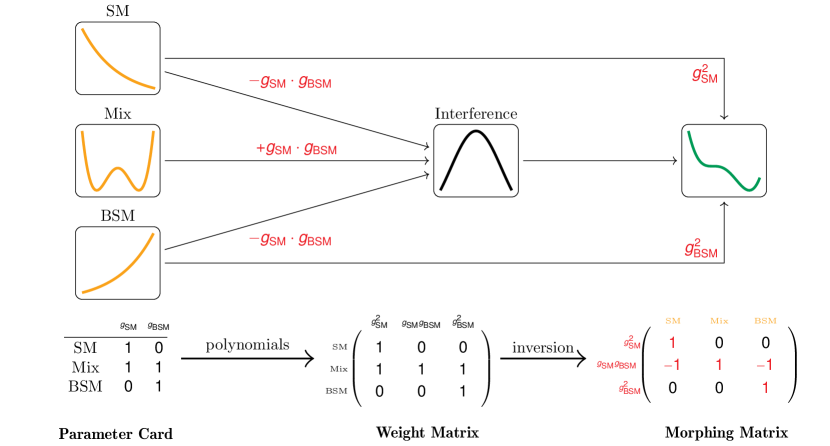
(a)

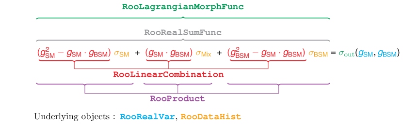
(b)

Figure 2: Schema showing the design of RooLagrangianMorphFunc class in RooFit for a simple case involving and effective Lagrangian with two parameters $g_{\text{SM}}$ and $g_{\text{BSM}}$. The cross section $\sigma_{\text{out}}$ is a distribution of an observable and defined for any ($g_{\text{SM}},g_{\text{BSM}}$) in terms of the input templates of the observable denoted by $\{\sigma_{\text{SM}},\sigma_{\text{Mix}},\sigma_{\text{BSM}}\}$. In the above, the observable distributions correspond to $(g_{\text{SM}},g_{\text{BSM}})=\{(1,0),(1,1),(0,1)\}$ respectively.

The RooLagrangianMorphFunc class in RooFit implements the Effective Lagrangian Morphing method, as derived in Section 2. The morphing distribution can be constructed for an arbitrary number of parameters $\vec{g}$ as long as the required number of non-degenerate samples are provided as an input to the morphing function. The morphed distribution provides a continuous description of the observable distribution in the parameter space, as spelled out in Eq. (10). The RooLagrangianMorphFunc implements the morphing as a sum of functions where each of the function is given by a RooLinearCombination object. The RooLinearCombination class implements the underlying summation of weight involved for each template as a Kahan sum to reduce loss of numeric precision that may occur in the repeated addition of a large number of summation terms.

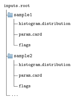
Figure 3: Expected structure of input ROOT file provided to the morphing function

To streamline the creation of a morphing function, the relevant configuration required are provided by the user through a RooLagrangianMorphFunc::Config object to configure the observable name, necessary parameters, coupling structures, and the input templates required to define a morphing function. Once created, the morphing function provides a description of the observable distribution for any coordinate in the parameter space.

The user is required to provide non-degenerate distributions of the observable at a set of coordinates (corresponding to $\sigma_{A}$, $\sigma_{B}$, …in Eq. (10)) and the corresponding parameter card which is used by the class to construct the morphed distribution in terms of the parameters $\vec{g}$. The input data are expected to be structured in the manner shown in Fig. 3, where sample1, sample2, and so on correspond to the different input folders (TFolder) and the histogram_distribution represents the template distribution that is picked up the morphing function (TH1). The param_cards (TH1 with labeled axis) contain the truth parameter values for the corresponding sample. The axis label correspond to the parameter names and the entry for the corresponding parameter is the truth value. The flags (TH1 with bin labels) contain the information of powers of $\Lambda^{-2}$ that is included in the simulated sample. The flags axis is given by {nNP0, nNP1, nNP2, ..} which corresponds to parameterss to track the contributions of $\Lambda^{-2}$. This is used to represent if the simulated sample is solely comprised of the SM contribution {nNP0=1, nNP1=0, nNP2=0}, SM-BSM interference {nNP0=0, nNP1=1, nNP2=0}, BSM-BSM interference {nNP0=0, nNP1=0, nNP2=1}, or a mix of them {nNP0=1, nNP1=1, nNP2=1}.

3.1 Usage

The construction of a morphing function is efficient with the most expensive steps in typical cases being the matrix inversion of the morphing matrix as represented in Eq. (9) to obtain the weight matrix and the I/O of the ROOT file containing the input templates. This inversion needs to be done only once at the initialization phase. Here both the linear and quadratic BSM operator terms are considered and hence the number of terms in the polynomial scales as given in Eq. (21). The dependence of initializing a morphing function and the evaluation time of the morphing function with the number of EFT parameters is shown in Fig. 4.

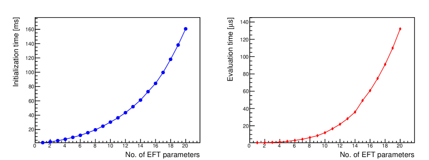
Figure 4: The dependence of the initialization and evaluation CPU time as a function of number of parameters of the morphing function. The estimate for the initialization time corresponds to the median value of the initialization called executed 5000 times. The evaluation time corresponds to the median of 5000 calls to the morphing function evaluation at randomly chosen parameter values.

The number of input template distributions required depends on the number of terms in the polynomial relation. For $n$ parameters with single insertion of EFT operators in the Feynman diagram the total number of samples $N$, that is required to construct the morphing distribution is given by,

$$N=\begin{cases}n+1&\text{, for linear terms in the BSM operators}\\ \frac{\displaystyle n^{2}+3n+2}{\displaystyle 2}&\text{, for linear \& quadratic BSM operator terms}\\ \end{cases}$$ (21)

To construct the morphing function C++ object, all input templates and their sampling coordinates in the parameter space must be specified in one transaction to the constructor. For ease of use, the RooLagrangianMorphFunc object can be configured with a RooLagrangianMorphFunc::Config which can be initialized step-by-step by the user adding one at a time the relevant couplings, input sample names, and the path to the ROOT file containing the input templates to the morphing function as shown in the example 1. Alternatively, the morphing function can be constructed through through the RooWorkspace factory language, as shown in the example 2 where a named-argument syntax compared to that of other RooFit operator classes can be used to structure the input information. The snippets for the example usage of the morphing function with a single and multi-parameter use case are taken from the tutorials available within ROOT.

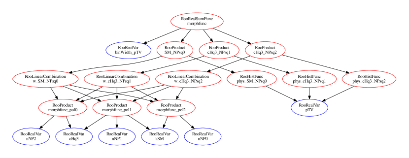
Figure 5: Tree structure of dependency graph of the underlying RooFit objects in the morphing function used in the 1D example.

Example use case with one morphing parameter

A minimal example of the Lagrangian morphing use case is when one parameter affects one distribution. In this example, a $2\to 2$ process is modelled following the derivation in Eq. (6) and (2.2). The process in question is $pp\to WH$ with $H\to bb$, generated with MadGraph5 [11], and a single non-SM operator ($\mathcal{O}_{\text{BSM}}$) $\mathcal{O}^{(3)}_{Hq}$ is chosen from the Warsaw basis [12], using the SMEFTsim model [13, 14] where the single insertion of EFT operators per diagram is considered. This corresponds to the scenario given by Eq. (4) with $(g_{SM},g_{\text{BSM}})=(1,\texttt{cHq3})$. To construct the morphing function for this case three non-degenerate input distributions are required. The sample provided as inputs to the morphing are the SM contribution ($\propto g_{SM}^{2}$), the interference of the operator with SM ($\propto g_{SM}g_{BSM}$), and the squared order contribution of the operator for $c^{(3)}_{Hq}=1.0$ ($\propto g_{BSM}^{2}$) generated using the $\texttt{NP}^{\wedge}\texttt{2==x}$ syntax where x is 0,1, or 2 respectively. The computational graph of RooFit function objects built by the morphing function is shown in Fig. 5. The input distributions as well as the predictions computed by the morphing functions are shown in Fig. 6.

The code snippet required to perform this computation using RooLagrangianMorphFunc is shown in Listing 1. The corresponding RooWorkspace factory interface usage, which can be used as an alternative means to the same end, is shown in Listing 2.

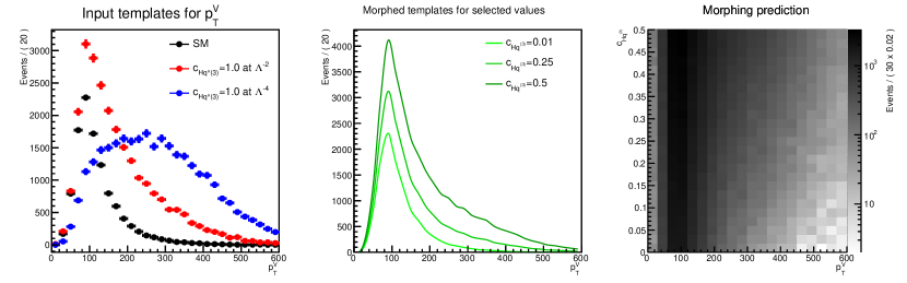
Figure 6: Example of the Lagrangian morphing for a one parameter case. The input distributions are shown on the left. The morphing prediction for select parameter values is shown in the center. The continuous description of the morphing function as a function of the parameter is shown in right.

Listing 1: Setup for a simple, one-dimensional morphing. The RooFit classes shown in the diagram in Fig. 2 are color-coded here accordingly.

     // usage of RooLagrangianMorphFunc for simple case  // prepare inputs    // necessary strings for inputs to morphing function  std::string infilename = "inputs/input_histos.root";  std::string obsname = "pTV";  std::vector<std::string> samples = {"SM_NPsq0","cHq3_NPsq1","cHq3_NPsq2"};    // create relevant parameters  RooRealVar cHq3("cHq3","cHq3",0,-10,10);  RooRealVar sm("SM","SM",1);  // Set NewPhysics order of parameter  cHq3.setAttribute("NewPhysics",true);    // Setup config object  RooLagrangianMorphFunc::Config config;  config.couplings.add(cHq3);  config.couplings.add(sm);  config.fileName = infilename.c_str();  config.observableName = obsname.c_str();  config.folderNames = samples;    // Setup morphing function  RooLagrangianMorphFunc morphfunc("morphfunc","morphfunc", config);     

Listing 2: Setup for a simple, one-dimensional morphing using the RooWorkspace factory interface.

     //RooLagrangianMorphFunc in the RooWorkspace factory interface  ws.factory("lagrangianmorph::morph(                     $fileName(’inputs/input_histos.root’),                     $observableName(’pTV’),                     $couplings({cHq3[0,1],SM[1]}),                     $NewPhysics(cHq3=1),                     $folders({’SM_NPsq0’,’cHq3_NPsq1’,’cHq3_NPsq2’}))");     

Multiple parameter use case

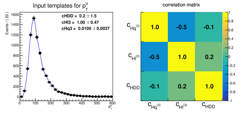
Figure 7: Example of the Lagrangian morphing for a multi-parameter use case. The figure shows the comparison of a fit to a pseudo dataset generated at ${c_{HDD}=0.2,c^{(3)}_{Hl}=1.0,c^{(3)}_{Hq}}=0.01$ as well as the correlation matrix.

The usage RooLagrangianMorphFunc class can be extended to handle arbitrary complexity in parameters and observable distributions simultaneously modelling multiple 1D distributions. This example uses the same process as Section 3.1, but this time, three different operators are introduced: $\mathcal{O}^{(3)}_{Hq}$, $\mathcal{O}^{(3)}_{Hl}$, and $\mathcal{O}_{HDD}$ with three corresponding Wilson coefficients as parameters $c^{(3)}_{Hq}$, $c^{(3)}_{Hl}$, and $c_{HDD}$. Following Eq. (21) 10 input samples are required as input templates to the morphing samples for this example. The 10 samples used here as inputs correspond to four types,

• SM - the sample of corresponding to the $g_{SM}^{2}$ Eq. (4) generated using $\texttt{NP}^{\wedge}\texttt{2==0}$.

• SM-BSM Interference - three samples of the form $g_{BSM}g_{SM}$ generated using $\texttt{NP}^{\wedge}\texttt{2==1}$ and by setting one of $c^{(3)}_{Hq}$, $c^{(3)}_{Hl}$, $c_{HDD}$ to $c=1.0$ and the remaining ones to $c=0.0$.

• BSM Square - three samples of the form $g_{BSM}^{2}$ generated using $\texttt{NP}^{\wedge}\texttt{2==2}$ and by setting one of $c^{(3)}_{Hq}$, $c^{(3)}_{Hl}$, $c_{HDD}$ to $c=1.0$ and the remaining ones to $c=0.0$.

• BSM-BSM Interference - three samples including the contribution of $g_{BSM_{i}}g_{BSM_{j}},g_{BSM_{i}}^{2},g_{BSM_{j}}^{2}$ $(i\neq j)$ generated using $\texttt{NP}^{\wedge}\texttt{2==2}$ and by setting two of $c^{(3)}_{Hq}$, $c^{(3)}_{Hl}$, $c_{HDD}$ to $c=1.0$ and the remaining ones to $c=0.0$.

The morphing distribution for a given parameter point is shown in Fig. 7.

Other parametrization scenarios

Ratio of Polynomials

As discussed in Section 2.5 the parameterisation for the cross-section can be modelled as a rational polynomial in the parameters when modelling separately the EFT behaviour of the of a narrow s-channel resonance and branching ratio as discussed in 18. The total cross-section in this scenario can be represented with the new RooRatio class which provides the option to build products and ratio of individual RooAbsReal function objects. To this end, the RooLagrangianMorphFunc implementation provides a dedicated makeRatio method to construct the ratio of morphing functions, which is showcased in Listing 3. The same can also be achieved with existing morphing functions. The syntax for this is shown in Listing 4, using the RooWorkspace factory interface.

Listing 3: Usage of the makeRatio method to construct a ratio of morphing functions.

     // RooRatio to setup up ratio of morphing functions  // morphfunc_prod --> function to model production EFT  // morphfunc_partial_width --> function to model partial width EFT  // morphfunc_total_width --> function to model total width EFT    // Setup numerator and denominator functions  RooArgList nr(morphfunc_prod,morphfunc_partial_width);  RooArgList dr(morphfunc_total_width);    // create ratio  auto ratio = RooLagrangianMorphFunc::makeRatio("ratio","ratio", nr, dr);     

Listing 4: Creation of a ratio of two morphing functions with the RooWorkspace factory interface.

     // RooRatio to setup up ratio of morphing functions  // in RooWorkspace factory interface  ws.factory("Ratio::ratio({morphfunc_prod,morphfunc_partial_width},                             {morphfunc_total_width});     

Taylor Expansion

The RooPolyFunc::taylorExpand method provides the Taylor expansion of any function with respect to a set of parameters with subsequent truncation at either first or second order for improved interpretability of the result. Listings 5 and 6 shows the usage of the truncated Taylor expansion formalism in C++ and the workspace factory language respectively.

Listing 5: Usage of the automatic Taylor expansion to obtain a morphing function at quadratic order based on a ratio of cross sections and branching ratios.

     // RooRatio to setup up ratio of morphing functions  // in RooWorkspace factory interface  // prodxBR --> RooRatio to model EFT in production & branching ratio  // truncating second-order Taylor expansion of prodxBR w.r.t (par1, par2)  // around 0.0 for both parameters  auto prodxBR_taylor = RooPolyFunc::taylorExpand("prodxBR_taylor",                                                  "prodxBR_taylor",                          // function to Taylor expand                                                  prodxBR,                          // parameters to Taylor expand around                                                 RooArgList(par1,par2),                          // expand around parameter coordinate,                          // one value of all parameters (0.0)                          // or vector ({0.0,0.0})                                                  0.0,                          //truncation order of expansion                                               2);     

Listing 6: Usage of the automatic Taylor expansion with the RooWorkspace factory interface.

     // RooRatio to setup up ratio of morphing functions  // in RooWorkspace factory interface  ws.factory("taylorexpand::prodxBR_taylor(prodxBR,{par1,par2},0.0,2);

References

- [1] The ATLAS Collaboration, “A morphing technique for signal modelling in a multidimensional space of coupling parameters”, ATL-PHYS-PUB-2015-047, CERN, Geneva, Nov, 2015. CDS:2066980.
- [2] LHC Higgs Cross Section Working Group, LHC Higgs Cross Section Working Group, “Handbook of LHC Higgs Cross Sections: 4. Deciphering the Nature of the Higgs Sector”, arXiv:1610.07922 [hep-ph].
- [3] W. Verkerke and D. P. Kirkby, “The RooFit toolkit for data modeling”, eConf C0303241 (2003) MOLT007 arXiv:physics/0306116 [physics].
- [4] ATLAS Collaboration, “Constraints on Higgs boson properties using production in 36.1 fb-1 of = 13 TeV collisions with the ATLAS detector”, arXiv:2109.13808 [hep-ex].
- [5] ATLAS Collaboration, “ Properties of Higgs Boson Interactions with Top Quarks in the and Processes Using with the ATLAS Detector”, Phys. Rev. Lett. 125 (Aug, 2020) 061802.
- [6] ATLAS Collaboration, “Test of CP invariance in vector-boson fusion production of the Higgs boson in the channel in proton–proton collisions at = 13 TeV with the ATLAS detector”, Physics Letters B 805 (2020) 135426 ScienceDirect:S0370269320302306.
- [7] CMS Collaboration, “Measurements of Production and the CP Structure of the Yukawa Interaction between the Higgs Boson and Top Quark in the Diphoton Decay Channel”, Phys. Rev. Lett. 125 no. 6, (2020) 061801 arXiv:2003.10866 [hep-ex].
- [8] CMS Collaboration, “Analysis of the CP structure of the Yukawa coupling between the Higgs boson and leptons in proton-proton collisions at = 13 TeV”, arXiv:2110.04836 [hep-ex].
- [9] N. Berger et al., “Simplified Template Cross Sections - Stage 1.1”, arXiv:1906.02754 [hep-ph].
- [10] ATLAS Collaboration, “Combined measurements of Higgs boson production and decay using up to fb-1 of proton-proton collision data at TeV collected with the ATLAS experiment”, Tech. Rep., CERN, Geneva, Nov, 2021. CDS:2789544.
- [11] J. Alwall, M. Herquet, F. Maltoni, O. Mattelaer, and T. Stelzer, “MadGraph 5 : Going Beyond”, JHEP 06 (2011) 128 arXiv:1106.0522 [hep-ph].
- [12] B. Grzadkowski, M. Iskrzynski, M. Misiak, and J. Rosiek, “Dimension-Six Terms in the Standard Model Lagrangian”, JHEP 10 (2010) 085 arXiv:1008.4884 [hep-ph].
- [13] I. Brivio, Y. Jiang, and M. Trott, “The SMEFTsim package, theory and tools”, JHEP 12 (2017) 070 arXiv:1709.06492 [hep-ph].
- [14] I. Brivio, “SMEFTsim 3.0 — a practical guide”, JHEP 04 (2021) 073 arXiv:2012.11343 [hep-ph].