Sparse Graph Learning with Spectrum Prior for Deep Graph Convolutional Networks

Abstract

A graph convolutional network (GCN) employs a graph filtering kernel tailored for data with irregular structures. However, simply stacking more GCN layers does not improve performance; instead, the output converges to an uninformative low-dimensional subspace, where the convergence rate is characterized by the graph spectrum—this is the known over-smoothing problem in GCN. In this paper, we propose a sparse graph learning algorithm incorporating a new spectrum prior to compute a graph topology that circumvents over-smoothing while preserving pairwise correlations inherent in data. Specifically, based on a spectral analysis of multilayer GCN output, we derive a spectrum prior for the graph Laplacian matrix ${\mathbf{L}}$ to robustify the model expressiveness against over-smoothing. Then, we formulate a sparse graph learning problem with the spectrum prior, solved efficiently via block coordinate descent (BCD). Moreover, we optimize the weight parameter trading off the fidelity term with the spectrum prior, based on data smoothness on the original graph learned without spectrum manipulation. The output ${\mathbf{L}}$ is then normalized for supervised GCN training. Experiments show that our proposal produced deeper GCNs and higher prediction accuracy for regression and classification tasks compared to competing schemes.

Index Terms—  Sparse graph learning, graph convolutional networks, graph signal processing

1 Introduction

Given a defined graph structure, graph convolutional networks (GCN) [1] perform graph filtering and point-wise non-linear operations (e.g., ReLU) in a sequence of neural layers for different tasks, such as graph signal interpolation, denoising, and node classification [1, 2, 3]. However, it has been observed that node representations become indistinguishable (known as over-smoothing) and prediction performance quickly degrades as the number of layers grows [4, 5]. This undesirable phenomenon limits GCN’s ability to learn appropriate representations from high-order neighborhood and motivates recent research to alleviate the over-smoothing problem [6, 7, 8, 9].

Existing works can be classified into two categories depending on whether the graph topology is modified. The first category of methods focus on novel network architecture designs given a fixed graph, e.g., using skip connections to combine features with various receptive fields [10], residual link and identity mapping to enable generalized graph filtering [6], and geometric aggregation to capture long-range dependencies in the graph [7].

On the other hand, the second category of methods stress the importance of graph choice in alleviating over-smoothing. [8] theoretically showed that the GCN output approaches an invariant subspace ${\mathcal{M}}$ spanned by the first eigenvector of the normalized graph Laplacian matrix $\tilde{{\mathbf{L}}}$—the subspace is uninformative beyond the number of connected components and node degrees. Convergence rate of the distance $d_{{\mathcal{M}}}$ between the GCN output and ${\mathcal{M}}$ is characterized by the graph spectrum of $\bar{{\mathbf{L}}}$, i.e., $\bar{{\mathbf{L}}}$’s eigenvalues determined by the graph topology.

To slow down convergence, [8] analyzed an upper bound for $d_{{\mathcal{M}}}$ determined by “eigen-gap”: the difference between the first and second dominant eigenvalues of matrix ${\mathbf{P}}={\mathbf{I}}-\tilde{{\mathbf{L}}}$—typically the first two eigenvalues of $\tilde{{\mathbf{L}}}$. Given that sparser graphs in general have smaller eigen-gaps (e.g., a complete unweighted graph has the maximum eigen-gap $2$), [8] showed that for random Erdö-Rényi graphs with edge probability $p$, sparser graphs (smaller $p$) converge to the aforementioned subspace at a slower pace. Similar in approach to achieve graph sparsity, [9] randomly removed edges from a pre-chosen graph topology in layers during training, resulting in more expressiveness in the trained GCNs. However, these methods implicitly optimized eigen-gaps by sparsifying graphs heuristically and may remove strong correlation edges that are essential for effective graph filtering, resulting in sub-optimal GCN performance.

In contrast, in this paper we propose a sparse graph learning algorithm incorporating a new spectrum prior to mitigate over-smoothing while preserving pairwise correlations inherent in data, resulting in deeper and more expressive GCNs. Specifically, inspired by the spectral analysis of multilayer GCN in [8], we derive a new spectrum prior for ${\mathbf{L}}$ to robustify the model expressiveness against over-smoothing. Given empirical covariance matrix $\bar{{\mathbf{C}}}$ computed from observable data, we formulate a sparse graph learning problem combining the graphical lasso (GLASSO) objective [13] with the new spectrum prior, which can be solved efficiently using a variant of block coordinate descent (BCD) [14]. Moreover, we optimize the weight parameter trading off the GLASSO objective with the spectrum prior, based on observable data smoothness with respect to (w.r.t.) the original graph learned without spectrum manipulation.

Compared with competing schemes [8, 9], by directly optimizing the spectrum we avoid random dropping of strong correlation edges, and thus enhance prediction accuracy for regression and classification tasks. Moreover, the designed spectrum prior considers the overall eigenvalue distribution rather than the eigen-gap alone, which is more effective in preserving GCN expressiveness. Different from graph learning algorithms in [13, 15, 16, 17, 18] that compute a most likely sparse inverse covariance matrix (interpreted as a generalized graph Laplacian matrix), we additionally incorporate the spectrum prior to combat over-smoothing towards deeper GCNs.

The learned graph is normalized and used for supervised GCN training. Experiments show that our proposal produced deeper GCN models with improved performance compared to existing schemes [6, 7, 8, 9]. We summarize our contributions as follows.

1. We design a new spectrum prior for graph Laplacian ${\mathbf{L}}$ to robustify GCN expressiveness against over-smoothing based on a spectral analysis of multilayer GCN output.

2. We formulate a sparse graph learning problem incorporating the proposed spectrum prior, solved efficiently to preserve pairwise correlation while promoting a desirable spectrum.

3. We optimize the weight parameter, trading off the GLASSO objective with the new spectrum prior, for optimal performance in different learning tasks.

2 Preliminaries

2.1 Notations

An undirected weighted graph ${\mathcal{G}}({\mathcal{V}},{\mathcal{E}},{\mathbf{W}})$ is defined by a set of $N$ nodes ${\mathcal{V}}=\{1,\ldots,N\}$, edges ${\mathcal{E}}=\{(i,j)\}$, and a symmetric adjacency matrix ${\mathbf{W}}$. $W_{i,j}\in\mathbb{R}$ is the edge weight if $(i,j)\in{\mathcal{E}}$, and $W_{i,j}=0$ otherwise. Self-loops may exist, in which case $W_{i,i}\in\mathbb{R}$ is the weight of the self-loop for node $i$. Diagonal degree matrix ${\mathbf{D}}$ has diagonal entries $D_{i,i}=\sum_{j}W_{i,j},\forall i$. A combinatorial graph Laplacian matrix ${\mathbf{L}}$ is defined as ${\mathbf{L}}\triangleq{\mathbf{D}}-{\mathbf{W}}$, which is positive semi-definite (PSD) for a positive graph [19]. If self-loops exist, then the generalized graph Laplacian matrix ${\mathcal{L}}$, defined as ${\mathcal{L}}\triangleq{\mathbf{D}}-{\mathbf{W}}+\text{diag}({\mathbf{W}})$, is typically used.

2.2 Vanilla GCN

For a given graph ${\mathcal{G}}({\mathcal{V}},{\mathcal{E}},{\mathbf{W}})$, a GCN [1] associated with ${\mathcal{G}}$ is defined as follows. Denote by $\widetilde{{\mathbf{W}}}\triangleq{\mathbf{W}}+{\mathbf{I}}$ and $\widetilde{{\mathbf{D}}}\triangleq{\mathbf{D}}+{\mathbf{I}}$ the adjacency and degree matrices augmented with self-loops, respectively. The augmented normalized Laplacian [20] is defined by $\widetilde{{\mathbf{L}}}\triangleq{\mathbf{I}}-\widetilde{{\mathbf{D}}}^{-1/2}\widetilde{{\mathbf{W}}}\widetilde{{\mathbf{D}}}^{-1/2}$, and we set ${\mathbf{P}}\triangleq{\mathbf{I}}-\widetilde{{\mathbf{L}}}$. Let $L,C\in\mathbb{N}^{+}$ be the layer and channel sizes, respectively. With weights $\mathbf{\Theta}^{(l)}\in\mathbb{R}^{C\times C}$, $l\in\{1,\ldots,L\}$, the GCN is defined by $f=f_{L}\circ\dots\circ f_{1}$ where $f_{l}:\mathbb{R}^{N\times C}\mapsto\mathbb{R}^{N\times C}$ is defined by $f_{l}({\mathbf{X}})\triangleq\sigma({\mathbf{P}}{\mathbf{X}}\mathbf{\Theta}^{(l)})$, where $\sigma$ denotes the nonlinear activation operator $\operatorname{ReLU}$.

3 Spectral Analysis

Based on the spectral analysis of multilayer GCN output in [8], we discuss the motivation of sparse graph learning with a spectrum prior to alleviate over-smoothing and induce deeper GCNs. First, we show that the convergence of GCN output to a low-dimensional invariant subspace is characterized by the graph spectrum. To robustify model expressiveness, we propose a linear spectrum prior, which will be incorporated into a sparse graph learning algorithm in the sequel.

3.1 Oversmoothing in Multilayer GCN

As defined in Sec.2.2, for a multilayer GCN model associated with ${\mathcal{G}}$, each layer $f_{l}({\mathbf{X}})\triangleq\sigma({\mathbf{P}}{\mathbf{X}}\mathbf{\Theta}^{(l)})$ consists of three basic operators: the graph operator ${\mathbf{P}}$, the filter $\mathbf{\Theta}^{(l)}$, and the activation $\sigma$. As proved in [8], each of the three operators leads to a decrease of the distance between the output of $l$-th layer ${\mathbf{X}}^{(l)}$ and the invariant subspace ${\mathcal{M}}$. Here, we focus on the graph operator ${\mathbf{P}}$, which is determined by the graph topology.

Specifically, denote by $\{{\mathbf{v}}_{1},...,{\mathbf{v}}_{N}\}$ the orthonormal eigenvectors of ${\mathbf{P}}$ corresponding to eigenvalues $\lambda_{1}\leq\dots\leq\lambda_{N}$. Suppose ${\mathcal{G}}$ has $M$ connected components. Then, we have $\lambda\triangleq\max_{n=1,\ldots,N-M}|\lambda_{n}|<1$ and $\lambda_{N-M+1}=\dots=\lambda_{N}=1$. We can then uniquely write ${\mathbf{X}}\in\mathbb{R}^{N\times C}$ as ${\mathbf{X}}=\Sigma_{n=1}^{N}{\mathbf{v}}_{n}\otimes{\mathbf{w}}_{n}$, where ${\mathbf{w}}_{1},\dots,{\mathbf{w}}_{n}\in\mathbb{R}^{C}$ are the coefficients w.r.t. the basis $\{{\mathbf{v}}_{1},...,{\mathbf{v}}_{N}\}$, and $\otimes$ is the Kronecker product. When applying the operator ${\mathbf{P}}$ to ${\mathbf{X}}$, the distance to the invariance space ${\mathcal{M}}$ is given by

$$d_{{\mathcal{M}}}^{2}({\mathbf{P}}{\mathbf{X}}) =\Sigma_{n=1}^{N-M}||\lambda_{n}{\mathbf{w}}_{n}||^{2}$$ (1)

$$\leq\Sigma_{n=1}^{N-M}\lambda^{2}||{\mathbf{w}}_{n}||^{2}=\lambda^{2}d_{{\mathcal{M}}}^{2}({\mathbf{X}}),$$ (2)

which shows that the graph operator ${\mathbf{P}}$ reduces the distance to the invariance space ${\mathcal{M}}$ at a rate characterized by the graph spectrum $\lambda_{n}$ for $n\in\{1,\dots,N-M\}$.

3.2 Spectrum Prior to Alleviate Over-smoothing

For given coefficients $\{{\mathbf{w}}_{1},\dots,{\mathbf{w}}_{N-M}\}$, to slow down the convergence to ${\mathcal{M}}$, the eigenvalues should be optimized as

$$\max_{\lambda_{1},\ldots,\lambda_{N-M}}\Sigma_{n=1}^{N-M}\lambda_{n}^{2}||{\mathbf{w}}_{n}||^{2},\mbox{s.t.}~{}~{}-1<\lambda_{1}\leq\dots\leq\lambda_{N-M}<1,$$ (3)

where the objective depends on the spectrum of ${\mathbf{P}}$ and the coefficient ${\mathbf{w}}_{n}$ of feature ${\mathbf{X}}$. To derive a spectrum prior as a function of ${\mathbf{L}}$, we relate $\lambda_{n}$ and ${\mathbf{w}}_{n}$ to the spectrum property of ${\mathbf{L}}$ as follows.

First, ${\mathbf{P}}$ is obtained from ${\mathbf{L}}$ via normalization to ensure ${\mathbf{P}}$ has eigenvalues in the range $[-1,1]$. Instead of using the normalization in [1], we adopt the following procedure to derive a linear spectrum prior for ${\mathbf{L}}$. Let $0\leq\mu_{1}\leq\dots\leq\mu_{N}$ be the eigenvalues of ${\mathbf{L}}$. $\mu_{1}{\mathbf{I}}_{N}$ is subtracted from ${\mathbf{L}}$, i.e., ${\mathbf{L}}_{0}={\mathbf{L}}-\mu_{1}{\mathbf{I}}_{N}$, so that the smallest eigenvalue of ${\mathbf{L}}_{0}$ is $0$, and correspondingly the largest eigenvalue of ${\mathbf{P}}$ is $1$. Then, ${\mathbf{L}}_{0}$ is scaled as

$${\mathbf{L}}_{\textrm{norm}}=\frac{2}{\mu_{\textrm{max}}}{\mathbf{L}}_{0},\quad{\mathbf{P}}={\mathbf{I}}-{\mathbf{L}}_{\textrm{norm}},$$ (4)

where $\mu_{\textrm{max}}>\mu_{N}$ is set to ensure that the eigenvalues of ${\mathbf{L}}_{\textrm{norm}}$ are in the range $[0,2]$. Thus,

$$\lambda_{n}=1-2(\mu_{N-n+1}-\mu_{1})/\mu_{\textrm{max}},$$ (5)

where $\mu_{N-n+1}$ has index $N-n+1$ because the eigenvalues of ${\mathbf{P}}$ and ${\mathbf{L}}$ have reverse orders. Moreover, from the procedure above we can see ${\mathbf{P}}$ and ${\mathbf{L}}$ share the same eigen-basis. Thus, the coefficient ${\mathbf{u}}_{n}$ of ${\mathbf{X}}$ w.r.t. the eigen-basis of ${\mathbf{L}}$ is given as ${\mathbf{w}}_{n}={\mathbf{u}}_{N-n+1}$.

Next, to examine ${\mathbf{u}}_{n}$, we assume that the model of ${\mathbf{X}}$ is a Gaussian Markov Random Field (GMRF) [21] w.r.t. ${\mathcal{G}}$, with covariance matrix $\mathbf{\Sigma}^{-1}={\mathbf{L}}+\delta{\mathbf{I}}$, where $1/\delta$ is interpreted as the variance of the DC component for ${\mathbf{X}}$ [22]. The expected energy of $\|{\mathbf{u}}_{n}\|^{2}$ is $\text{E}[\|{\mathbf{u}}_{n}\|^{2}]=1/(\delta+\mu_{n})$ [23]. With $\delta=0$, the objective (3) becomes

$$\max_{\mu_{M+1},...,\mu_{N}}\Sigma_{n=M+1}^{N}(1-\frac{2}{\mu_{\textrm{max}}}(\mu_{n}-\mu_{1}))^{2}/\mu_{n},$$ (6)

which can be further simplified to

$$\max_{\mu_{M+1},...,\mu_{N}}\Sigma_{n=M+1}^{N}(1+\frac{2\mu_{1}}{\mu_{\textrm{max}}})^{2}/\mu_{n}+(\frac{2}{\mu_{\textrm{max}}})^{2}\mu_{n}$$ (7)

and the objective function decreases monotonically when $\mu_{n}<\frac{\mu_{\textrm{max}}+2\mu_{1}}{2}$. By setting $\mu_{\textrm{max}}\geq 2(\mu_{N}-\mu_{1})$, the objective becomes $\min\Sigma_{n=M+1}^{N}\mu_{n}$. Since $\mu_{1},\ldots,\mu_{M}=0$, the objective is further simplified to $\min\|\boldsymbol{\mu}\|_{1}$, where $\boldsymbol{\mu}=[\mu_{1},\dots,\mu_{N}]$.

In summary, assuming the model of ${\mathbf{X}}$ is a GMRF specified by ${\mathbf{L}}$ with eigenvalues $0\leq\mu_{1}\leq\dots\leq\mu_{N}$, $\boldsymbol{\mu}=[\mu_{1},\dots,\mu_{N}]$, convergence to the invariant space ${\mathcal{M}}$ is slowed down via

$$\min_{{\mathbf{L}}}\quad\|\boldsymbol{\mu}\|_{1},$$ (8)

where $\mu_{\textrm{max}}\geq 2(\mu_{N}-\mu_{1})$ for ${\mathbf{L}}$ normalization to produce ${\mathbf{P}}$.

Relation to Weight Scaling Scheme in [8] Based on the upper-bound of $d_{{\mathcal{M}}}^{2}({\mathbf{P}}{\mathbf{X}})$ in (2), [8] proved that, with initial value ${\mathbf{X}}^{0}$, $d_{{\mathcal{M}}}({\mathbf{X}}^{(l)})$ satisfies $d_{{\mathcal{M}}}({\mathbf{X}}^{(l)})\leq(s\lambda)^{l}d_{{\mathcal{M}}}({\mathbf{X}}^{0})$, where $s:=\sup_{l=1,\ldots L}s_{l}$ and $s_{l}$ is the maximum singular value of $\mathbf{\Theta}^{(l)}$. In particular, $d_{{\mathcal{M}}}({\mathbf{X}}^{(l)})$ exponentially converges to 0 if $s\lambda<1$. Hence, [8] proposed to normalize the weight $\mathbf{\Theta}^{(l)}$ so that $s_{l}\lambda>1$ in order to slow down the convergence to the invariant subspace.

However, since the eigenvalues of ${\mathbf{P}}$ are generally different from $\lambda$, the upper bound of $d_{{\mathcal{M}}}^{2}({\mathbf{P}}{\mathbf{X}})$ in (2) is so loose that the weight scaling scheme proposed in [8] has limited effect in avoiding over-smoothing. In contrast, our proposed spectrum prior in (8) considers the entire spectrum instead of only the second largest $\lambda$, leading to improved performance as validated in our experiments.

4 Sparse Graph Learning with Spectrum Prior for GCN Training

In this section, we propose a new sparse graph learning algorithm using the proposed graph spectrum prior. Further, we design a measure to optimally trade off pairwise correlation preservation with the spectrum prior, based on smoothness of observable data on the original graph learned without spectrum manipulation.

4.1 Problem Formulation

We incorporate the spectrum prior in (8) into the GLASSO formulation [13], resulting in the following graph learning objective:

$$\min_{\mathbf{L}\succeq\mathbf{0}}~{}~{}\text{Tr}(\mathbf{L\bar{{\mathbf{C}}}})-\log\det\mathbf{L}+\rho\;\|\mathbf{L}\|_{1}+\sigma\text{Tr}(\mathbf{L}),$$ (9)

where the spectrum prior is $\text{Tr}(\mathbf{L})=\|\boldsymbol{\mu}\|_{1}$. $\bar{{\mathbf{C}}}$ is the input empirical covariance matrix computed from observable data, $\rho>0$ is a shrinkage parameter for the $\ell_{1}$-norm of ${\mathbf{L}}$, and $\sigma$ is the weight for spectrum prior. Next, we discuss the computation of $\sigma$ to trade off the GLASSO objective with the spectrum prior.

4.2 Computing Tradeoff Parameter $\sigma$

Based on the smoothness of the observable data ${\mathbf{F}}\in\mathbb{R}^{N\times K}$ on the original graph learned given $\bar{{\mathbf{C}}}$ without spectrum manipulation, we determine weight $\sigma$ in (9) to trade off preservation of pairwise correlation inherent in $\bar{{\mathbf{C}}}$ with alleviation of over-smoothing. The idea is the following: if data ${\mathbf{F}}$ is smooth w.r.t. the original GLASSO output $\hat{{\mathbf{L}}}$ without spectrum prior ($\sigma=0$), then ${\mathbf{F}}$ has energy mostly in the invariant subspace ${\mathcal{M}}_{0}$ of $\hat{{\mathbf{L}}}$ spanned by the eigenvector of the lowest frequency. That means convergence to ${\mathcal{M}}_{0}$ has little impact on prediction accuracy, and hence the spectrum prior can be removed, i.e., $\sigma=0$. Otherwise, the spectrum prior should be assigned higher weight to slow down convergence.

To quantify signal smoothness, given the original GLASSO output $\hat{{\mathbf{L}}}$, we define the measure using a variant of the quadratic graph Laplacian regularizer (GLR) [24], i.e.,

$$\mathrm{M}_{\hat{{\mathbf{L}}}}({\mathbf{F}})=\frac{{\text{Tr}}({\mathbf{F}}^{\top}\hat{{\mathbf{L}}}{\mathbf{F}})}{\hat{\mu}_{N}{\text{Tr}}({\mathbf{F}}^{\top}{\mathbf{F}})},$$ (10)

which measures the smoothness of the data w.r.t. graph specified by $\hat{{\mathbf{L}}}$, normalized by the signal energy. $\hat{\mu}_{N}$ is the largest eigenvalue of $\hat{{\mathbf{L}}}$, used here to normalize $\mathrm{M}_{\hat{{\mathbf{L}}}}({\mathbf{F}})$ to the range $[0,1]$.

Weight $\sigma$ should increase monotonically with $\mathrm{M}_{\hat{{\mathbf{L}}}}({\mathbf{F}})$ in $[0,1]$, and thus we set $\sigma$ to be a scaled and shifted logit function [25]:

$$\sigma=\ln\left(\frac{1+\mathrm{M}_{\hat{{\mathbf{L}}}}({\mathbf{F}})}{1-\mathrm{M}_{\hat{{\mathbf{L}}}}({\mathbf{F}})}\right).$$ (11)

We see that when $\mathrm{M}_{\hat{{\mathbf{L}}}}({\mathbf{F}})$ is small, $\sigma$ is small, and when $\mathrm{M}_{\hat{{\mathbf{L}}}}({\mathbf{F}})$ approaches $1$, $\sigma$ approaches infinity.

4.3 Algorithm Design

Given computed $\sigma$ and the objective in (9), we design an algorithm as summarized in Algorithm 1. We call the algorithm Sparse Graph Learning with Spectrum Prior for GCN, named SGL-GCN.

By combining $\text{Tr}(\mathbf{L\bar{{\mathbf{C}}}})$ and $\sigma\text{Tr}(\mathbf{L})$ as $\text{Tr}(\mathbf{L(\bar{{\mathbf{C}}}+\sigma{\mathbf{I}})})$, we solve (9) iteratively using a variant of the block coordinate descent (BCD) algorithm [14]. Specifically, similarly done in [26], we solve the dual of GLASSO as follows. First, note that the $\ell_{1}$-norm in (9) can be written as

$$\|{\mathbf{L}}\|_{1}=\max_{\|{\mathbf{U}}\|_{\infty}\leq 1}~{}~{}\text{Tr}({\mathbf{L}}{\mathbf{U}})$$ (12)

where $\|{\mathbf{U}}\|_{\infty}$ is the maximum absolute value element of the symmetric matrix ${\mathbf{U}}$. The dual problem of GLASSO that seeks an estimated covriance matrix ${\mathbf{C}}={\mathbf{L}}^{-1}$ can now be written as

$$\min_{{\mathbf{C}}}~{}~{}-\log\det{\mathbf{C}},~{}~{}~{}\mbox{s.t.}~{}~{}\|{\mathbf{C}}-(\bar{{\mathbf{C}}}+\sigma{\mathbf{I}})\|_{\infty}\leq\rho.$$ (13)

To solve (13), we update one row-column pair of ${\mathbf{C}}$ in (13) in each iteration following optimization procedure in [15].

In summary, our algorithm to solve (9) is as follows. We minimize the GLASSO terms in (9) by solving its dual (13)—iteratively updating one row / column of ${\mathbf{C}}$ at a time. We repeat these two steps till convergence. Note that both steps are computed using covariance ${\mathbf{C}}$ directly, and thus inversion to graph Laplacian ${\mathbf{L}}={\mathbf{C}}^{-1}$ is not necessary until convergence, when we output a solution.

Algorithm 1 Sparse Graph Learning with Spectrum Prior for GCN

1:Empirical covariance matrix $\bar{{\mathbf{C}}}$, observable data ${\mathbf{F}}$

2:Graph operator ${\mathbf{P}}$ for GCN model

3:Obtain the original GLASSO output $\hat{{\mathbf{L}}}$ given $\bar{{\mathbf{C}}}$ with $\sigma=0$ via graph learning algorithm described in Sec 4.3.

4:Compute the weight value $\sigma$ given $\hat{{\mathbf{L}}}$ and ${\mathbf{F}}$.

5:Obtain the sparse graph learning output ${\mathbf{L}}$ incorporating GLASSO objective and spectrum prior via algorithm in Sec 4.3.

6:Normalize ${\mathbf{L}}$ with (4) to produce ${\mathbf{P}}$.

7:Use ${\mathbf{P}}$ for GCN training.

5 Experiments

We conducted experiments to validate our graph learning proposal that alleviates over-smoothing and improves prediction accuracy by comparing against recent proposals, including DropEdge [9], Oono’s scheme [8], GCNII [6] and Geom-GCN [7].

5.1 Dataset and Experiment Settings

For regression, we used the METR-LA dataset [27] containing traffic speed data in four months (from March 1st 2012 to June 30th 2012) from 207 sensors in the Los Angeles County. The sensors sampled the speed data every 5 minutes. Our task is to predict the current traffic speed using historical speed data in the past 50 minutes as the input feature. We randomly sampled 70% data for training, 20% for validation, and 10% for testing. The empirical covariance $\bar{{\mathbf{C}}}$ was computed using all the observations in the training data.

For node classification, we used Cornell, Texas, and Wisconsin datasets, which are from the WebKB dataset [7]. These dataset are web networks, where nodes and edges represent web pages and hyperlinks, respectively. The feature of each node is the bag-of-words representation of the corresponding page. We followed the experimental setting in [7] for node classification. $\bar{{\mathbf{C}}}$ was the inverse of the graph Laplacian constructed using node feature similarity. In particular, we constructed K-NN graph ($K=10$), with edge weights computed as $w_{ij}=\exp(-\|{\mathbf{f}}_{i}-{\mathbf{f}}_{j}\|^{2}/2\gamma)$ ($\gamma=5$), where ${\mathbf{f}}_{i}$ is the feature for node $i$.

For graph learning, sparsity parameter $\rho$ in (9) was set to $10^{-4}$. For normalization of ${\mathbf{L}}$, $\mu_{\textrm{max}}=11$ for METR-LA and $\mu_{\textrm{max}}=1$ for Web-KB. GCN training was implemented in PyTorch and optimized by Adam [28] with initial learning rate set to $0.01$ and weight decay set to $5e-5$. Our GCN model was consisted of $L$ GCN blocks ($L=[1,10]$) and two linear layers.

5.2 Validation of Weight Computation

To validate the proposed measure to compute $\sigma$, we set $\sigma\in\{0,1e1,1e-3\}$ and compared against the value computed via our proposed scheme, which was $0.0038$ for METR-LA dataset. Fig. 1 shows the results for GCN training using graph Laplacian matrices learned using different $\sigma$. Large $\sigma$, e.g. $1e1$, mitigated over-smoothing of the GCN model and achieved larger optimal layer number ($7$), but the learned graph deviated too far from $\bar{{\mathbf{C}}}$ and failed to achieve small MSE. On the other hand, small $\sigma$, e.g. $1e-3$ quickly reduced the MSE with few layers ($2$), but could not reduce MSE with more layers due to over-smoothing. Meanwhile, our proposed scheme with $\sigma=3.8e-3$ achieved the lowest MSE, indicating the importance of choosing an appropriate weight $\sigma$.

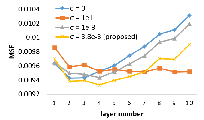
Fig. 1: MSE results with different layer sizes of GCN models using Laplacian matrices learned with different weighting factors. The proposed scheme balance the convergence rate and the covaraince preservation, achieving the lowest prediction error.

Table 1: MSE results ($\times 10^{-3}$) of META-LA dataset with different layer size of GCN models using different schemes.

Methods	2 layers	4 layers	8 layers
GCN [1]	10.76	11.81	17.38
DropEdge [9]	10.79	12.25	17.72
Oono’s [8]	10.79	11.89	17.32
SGL-GCN w/o spectrum	9.43	9.52	10.05
SGL-GCN	9.38	9.33	9.70

5.3 Comparison with State-of-the-Art Methods

We compared our method with competing schemes DropEdge [9] and Oono’s scheme [8] for traffic prediction task, and additionally included GCNII [6] and Geom-GCN [7] for node classification. The most related schemes are DropEdge and Oono’s method which modify graph topologies for GCN training. We used the same experimental settings for DropEdge with drop rate $p=0.3$ and Oono’s weight scaling with default ${\mathbf{s}}_{0}=1$. For Geom-GCN, three variants were included using different embedding methods, i.e., Isomap (Geom-GCN-I), Poincare (Geom-GCN-P), and struc2vec (Geom-GCN-S). For our proposal, $\sigma=0.9661,0.9147,0.9147$ for Wisconsin, Texas, and Cornell datasets, respectively.

The resulting MSE of META-LA dataset are shown in Table 1, where the optimal results are highlighted in bold font. We observe that our method had better performance in terms of slowing down over-smoothing and achieving higher prediction accuracy. Specifically, DropEdge achieved its best result at the second layer with MSE $0.0107$, while our method increased the optimal layer number to $4$ and achieved lower MSE $0.0093$. Moreover, by removing the spectrum prior in our proposal, i.e., SGL-GCN w/o spectrum in Table 1, the performance was degraded, validating the effectiveness of the spectrum prior.

The test accuracy of WebKB dataset are shown in Table 2. We selected the performance of the optimal layer number for each scheme. We see that our proposal outperformed the state-of-the-art methods in all three datasets. Comparing with DropEdge and Oono’s, we increased the accuracy by more than $20\%$, which clearly shows the importance of explicit spectrum optimization.

Table 2: Test accuracy (%) of WebKB dataset for different schemes.

Methods	Wisconsin	Texas	Cornell
GCN [1]	45.88	52.16	52.7
Dropedge [9]	61.62	57.84	50.2
Oono’s [8]	53.92	58.92	61.08
Geom-GCN-I [7]	58.24	57.58	56.76
Geom-GCN-P [7]	64.12	67.57	60.81
Geom-GCN-S [7]	56.67	59.73	55.68
GCNII [6]	81.57	77.84	76.49
SGL-GCN w/o spectrum	82.35	78.11	80.00
SGL-GCN	85.69	82.70	82.97

6 Conclusion

We propose a sparse graph learning algorithm with a new spectrum prior to alleviate over-smoothing problem of GCN model while preserving pairwise correlation inherent in data. Specifically, a new spectrum prior is designed to robustify the GCN expressiveness against over-smoothing, which is combined with the GLASSO objective for efficient sparse graph learning. The trade-off between the fidelity term and spectrum prior is balanced with the proposed measure that quantifies the data smoothness on the graph learned without spectrum manipulation. Compared to competing schemes, our proposal produced deeper GCNs with improved performance.

References

- [1] Thomas N. Kipf and Max Welling, “Semi-supervised classification with graph convolutional networks,” in International Conference on Learning Representations (ICLR), 2017.
- [2] Fenyu Hu, Yanqiao Zhu, Shu Wu, Liang Wang, and Tieniu Tan, “Hierarchical graph convolutional networks for semi-supervised node classification,” in International Joint Conference on Artificial Intelligence (IJCAI), 2019.
- [3] Tien Huu Do, Duc Minh Nguyen, and Nikos Deligiannis, “Graph auto-encoder for graph signal denoising,” in IEEE International Conference on Acoustics, Speech and Signal Processing (ICASSP). IEEE, 2020, pp. 3322–3326.
- [4] Qimai Li, Zhichao Han, and Xiao-Ming Wu, “Deeper insights into graph convolutional networks for semi-supervised learning,” in AAAI Conference on Artificial Intelligence (AAAI), 2018.
- [5] Guohao Li, Matthias Muller, Ali Thabet, and Bernard Ghanem, “Deepgcns: Can gcns go as deep as cnns?,” in International Conference on Computer Vision (ICCV), 2019, pp. 9267–9276.
- [6] Ming Chen, Zhewei Wei, Zengfeng Huang, Bolin Ding, and Yaliang Li, “Simple and deep graph convolutional networks,” in International Conference on Machine Learning (ICML). PMLR, 2020, pp. 1725–1735.
- [7] Hongbin Pei, Bingzhe Wei, Kevin Chen-Chuan Chang, Yu Lei, and Bo Yang, “Geom-gcn: Geometric graph convolutional networks,” in International Conference on Learning Representations (ICLR), 2020.
- [8] Kenta Oono and Taiji Suzuki, “Graph neural networks exponentially lose expressive power for node classification,” in International Conference on Learning Representations (ICLR), 2020.
- [9] Yu Rong, Wenbing Huang, Tingyang Xu, and Junzhou Huang, “Dropedge: Towards deep graph convolutional networks on node classification,” in International Conference on Learning Representations (ICLR), 2020.
- [10] Keyulu Xu, Chengtao Li, Yonglong Tian, Tomohiro Sonobe, Ken-ichi Kawarabayashi, and Stefanie Jegelka, “Representation learning on graphs with jumping knowledge networks,” in International Conference on Machine Learning (ICML). PMLR, 2018, pp. 5453–5462.
- [11] Carl D Meyer, Matrix Analysis and Applied Linear Algebra, SIAM, 2010.
- [12] Charles F Van Loan and G Golub, Matrix Computations (Johns Hopkins Studies in the Mathematical Sciences), Johns Hopkins University Press, 2012.
- [13] Jerome Friedman, Trevor Hastie, and Robert Tibshirani, “Sparse inverse covariance estimation with the graphical lasso,” Biostatistics (Oxford, England), vol. 9, pp. 432–41, 08 2008.
- [14] Stephen J SWright, “Coordinate descent algorithms,” Math. Program., vol. 151, no. 1, pp. 3–34, 2015.
- [15] Onureena Banerjee, Laurent El Ghaoui, and Alexandre d’Aspremont, “Model selection through sparse max likelihood estimation,” Journal of Machine Learning Research (JMLR), vol. 9, 08 2007.
- [16] Hilmi E Egilmez, Eduardo Pavez, and Antonio Ortega, “Graph learning from data under Laplacian and structural constraints,” in IEEE Journal of Selected Topics in Signal Processing, July 2017, vol. 11, no.6, pp. 825–841.
- [17] Wei Hu, Gene Cheung, Antonio Ortega, and Oscar C Au, “Multi-resolution graph Fourier transform for compression of piecewise smooth images,” in IEEE Transactions on Image Processing, January 2015, vol. 24, no. 1, pp. 419–433.
- [18] Fei Chen, Gene Cheung, and Xue Zhang, “Fast & robust image interpolation using gradient graph laplacian regularizer,” in IEEE International Conference on Image Processing (ICIP), 2021, pp. 1964–1968.
- [19] Gene Cheung, Enrico Magli, Yuichi Tanaka, and Michael K Ng, “Graph spectral image processing,” in Proceedings of the IEEE, May 2018, vol. 106, no.5, pp. 907–930.
- [20] Felix Wu, Amauri Souza, Tianyi Zhang, Christopher Fifty, Tao Yu, and Kilian Weinberger, “Simplifying graph convolutional networks,” in International Conference on Machine Learning (ICML). PMLR, 2019, pp. 6861–6871.
- [21] Havard Rue and Leonhard Held, Gaussian Markov random fields: theory and applications, Chapman and Hall/CRC, 2005.
- [22] Akshay Gadde and Antonio Ortega, “A probabilistic interpretation of sampling theory of graph signals,” in IEEE International Conference on Acoustics, Speech and Signal Processing (ICASSP). IEEE, 2015, pp. 3257–3261.
- [23] Jin Zeng, Gene Cheung, and Antonio Ortega, “Bipartite approximation for graph wavelet signal decomposition,” in IEEE Transactions on Signal Processing, July 2017, vol. 65, pp. 5466–5480.
- [24] J. Pang and G. Cheung, “Graph Laplacian regularization for inverse imaging: Analysis in the continuous domain,” in IEEE Transactions on Image Processing, April 2017, vol. 26, no.4, pp. 1770–1785.
- [25] James S Cramer, “The origins and development of the logit model,” Logit models from economics and other fields, pp. 149–158, 2003.
- [26] Saghar Bagheri, Gene Cheung, Antonio Ortega, and Fen Wang, “Learning sparse graph Laplacian with eigenvector prior via iterative glasso and projection,” in IEEE International Conference on Acoustics, Speech and Signal Processing (ICASSP), 2021, pp. 5365–5369.
- [27] Yaguang Li, Rose Yu, Cyrus Shahabi, and Yan Liu, “Diffusion convolutional recurrent neural network: Data-driven traffic forecasting,” in International Conference on Learning Representations (ICLR), 2018.
- [28] Diederik P Kingma and Jimmy Ba, “Adam: A method for stochastic optimization,” in International Conference on Learning Representations (ICLR), 2015.