Gradient-free Multi-domain Optimization for Autonomous Systems

Abstract

Autonomous systems are composed of several subsystems such as mechanical, propulsion, perception, planning and control. These are traditionally designed separately which makes performance optimization of the integrated system a significant challenge. In this paper, we study the problem of using gradient-free optimization methods to jointly optimize the multiple domains of an autonomous system to find the set of optimal architectures for both hardware and software. We specifically perform multi-domain, multi-parameter optimization on an autonomous vehicle to find the best decision-making process, motion planning and control algorithms, and the physical parameters for autonomous racing. We detail the multi-domain optimization scheme, benchmark with different core components, and provide insights for generalization to new autonomous systems. In addition, this paper provides a benchmark of the performances of six different gradient-free optimizers in three different operating environments. Our approach is validated with a case study where we describe the autonomous vehicle system architecture, optimization methods, and finally, provide an argument on gradient-free optimization being a powerful choice to improve performance of autonomous systems in an integrated manner.

I INTRODUCTION

The design of Cyber-Physical-Systems (CPS) includes a wide variety of engineering areas such as mechanical, electrical, control and decision making. Autonomous Systems, within CPS, has a wide variety of applications: Unmanned aerial vehicle (UAV), unmanned underwater vehicles (UUV), and autonomous vehicles (AV) to name a few. For an Autonomous System to function properly, core components such as autonomy algorithms (perception, planning, and prediction) [1], physical components, and low level control algorithms must work together. However, to find the optimal configuration for a good performance of an Autonomous System, there are multiple challenges that system designer must overcome. First, the right combination of core hardware components must be determined. This task is hard to solve because for each of these core components, there are usually more than dozens of either continuous or categorical parameters that could change the behavior of each component. This creates a massive combinatorial problem that cannot be solved manually by tuning for different parameters. This problem becomes even harder when evaluating a single combination is computationally, or manually expensive. In addition, clear measurements that define the overall performance of the autonomous system and in addition display a comparability for other autonomous system developer is needed. Lastly, due to the cyber-physical nature of Autonomous Systems, any simulation created will have to use models that have a certain discrepancy to real world behavior (e.g. sensor models, vehicle dynamics models), which creates a sim-to-real gap that leads to different performances on real hardware. In addition, choosing an objective function that might differ between simulation and real world might lead to unexpected behavior that ends up exploiting the simulation dynamics.

In order to overcome these issues we want to show that a deterministic and embarrassingly parallel optimization pipeline can be set up that derives optimal hardware and software configuration for autonomous systems. As an effort to push forward more generalizable optimization methods suitable for a wide range of systems, this work has three primary contributions.

1. We provide a scheme for gradient-free, multi-domain optimization of an autonomous system and provide case studies with specified target hardware, modular software, and a calibrated simulator of an autonomous race car.

2. We provide thorough benchmark evaluating the performance of different optimization techniques with focus on gradient free methods and describe a methodology for tuning a high-dimensional set of hyperparameters across multiple domains.

3. We provide insights in adapting and optimizing heterogeneous components of new autonomous systems in different domains.

In what follows, we demonstrate that the proposed multi-domain optimization is capable of finding optimal configurations for both hardware and software of an autonomous system. In Section II, we describe the problem statement and the design of our optimization pipeline. In Section III we provide the state of the art and place our solution in context with previous approaches. In Section IV, we describe the experimental setup and analysis of generated results. Lastly, in Section VI, we detail future work and conclusions.

II METHODOLOGY

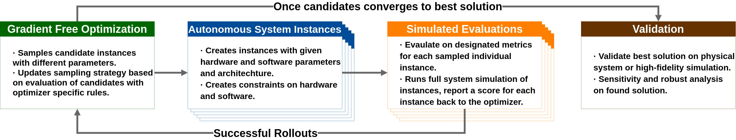
Figure 1: Proposed pipeline for autonomous systems optimization.

To solve the problem of creating an optimized autonomous system we propose the pipeline displayed in Figure 1. In the first step, the head node of the optimization samples candidate instances of solutions with different parameters according to some underlying sampling strategy. In the second step, a fixed number of parallel workers are created to receive the sampled candidate solutions and create an Autonomous System simulation instance for each of them. So far we have explored AVs, UUVs and UAVs as autonomous systems that are presented as standalone autonomous systems. An extension regarding e.g. connected systems can be done in the problem formulation but not was explored yet. In the third step each of the Autonomous System instances is now evaluated in a full system simulation. This simulation provides the environment, the virtual sensors, and the Autonomous System dynamics. After simulating each instance with the given candidate, the workers collects metrics on the performance of each instance and reports its findings back to the optimization head node where the iteration starts again for the next generation. This also updates the underlying sampling strategy that the head node uses. Once all candidates converged to a best solution, the optimization halts and provides a final candidate with the most performant combination of parameters. The solution could then be validated in either a high fidelity simulation environment or with real hardware.

II-A Problem Statement

We first loosely define an autonomous system as a system with: 1. intricate interaction between multiple components that produces complex dynamics; 2. variable hardware and/or software parameters that influence the overall performance on given metrics. Some examples of an autonomous system include: buildings with energy efficiency optimization, self-driving cars, unmanned aerial and underwater vehicles. The goal of the optimization framework is to find the best combination of parameters in the search space that increase the overall performance of the autonomous system. Mathematically, we define the objective of the optimization problem as:

$$\begin{array}[]{ll}\operatorname{minimize}&f(\theta)\\ \operatorname{\text{subject to}}&\theta\in\Theta\end{array}$$ (1)

Where $f(\Theta):\mathbb{R}^{n}\rightarrow\mathbb{R}$ is the objective function that measures the system’s performance on a metric, and a lower function value corresponds to a higher overall system performance. $\Theta$ is the concatenation of all feasible search space of all parameters being tuned. $\theta$ is a candidate sampled from $\Theta$. We do not assume the existence of a gradient and the convexity of the objective function. By defining the problem as stated we can use the proposed approach for optimizing autonomous systems of all kinds.

II-B Search Space

We divide the search space generally into three sub-spaces: Physical parameters, High-level decision-making parameters, and Low-level control parameters.

The physical parameters $\Theta_{p}$ are defined as the parameters that can be physically altered in an autonomous system. For example the mass of the system, the position of the center of gravity (CoG), the hardware components of the system etc. We further provide guidance on how to limit the range of these parameters, and how to initialize these parameters in the search in section V

The high-level decision-making parameters $\Theta_{dm}$ are defined as the parameters that governs the high level planning decisions of the autonomous system. For example, the importance an autonomous system takes to sacrifice robustness for performance (e.g. the magnitude of a slack variable in a constraint), the parameters in a neural network that controls an autonomous system end-to-end, or the creation of a trajectory (path planning) the system is trying to track.

The low-level control parameters $\Theta_{lc}$ are defined as the parameters that affect the low-level controller of the autonomous system. For example, the $k_{p}$, $k_{i}$ and $k_{d}$ parameter in an PID-controller or the optimization parameters in an MPC-controller.

In section IV, we provide a real world case study where all of the parameters in the concatenated search space for the system are clearly defined and discussed.

II-C Evaluation Criteria

The evaluation criteria depends on the specific system that’s being optimized. We assume the evaluation criteria to be a function that maps from the parameter search space $\mathbb{R}^{n}$ to a single or a vector of real numbers. The optimization process doesn’t necessarily optimize in only one dimension that measures performance. As long as the objective function satisfies the requirements, there could be multiple aspect of the autonomous system being optimized. For example, we can optimize the performance of an autonomous vehicle in terms of it’s fuel efficiency, in terms of power output, but also in terms of the computation efficiency of the on-board software. For a given set of parameters $\theta$ sampled from $\Theta$, we calculate the objective function $f(\theta)$ through simulation of the autonomous system, then the obtained score is returned to the optimizer to push the optimization forward for the next sample.

In section IV, we give clear and well-defined evaluation criteria on our real world case study.

II-D Optimization

Since we do not assume the convexity and smoothness, the upper bound of the dimension, and the existence of closed-form expression of the underlying dynamics, we use gradient-free, black-box optimization to solve the problem. A potential pitfall of this method of optimization on our target autonomous system is the potential existence of local optima, which creates inherent tension between exploration of the search space and exploitation of solutions. We discuss and analyze this failure mode in section V and IV.

In our experiments, we use the following optimization algorithms:

1. CMA (Covariance Matrix Adaptation) is an evolution strategy [2]. For each generation, CMA samples potential solutions in a multivariate normal distribution defined by a mean and covariance. The mean of the distribution is updated to maximize the likelihood of previously successful solutions based off of a fitness function that evaluates the quality of solution. The algorithm keeps track of two evolution paths (isotropic and anisotropic) based on the previous and current mean. The isotropic evolution path exploits the covariance matrix which helps the algorithm choose a better distribution for the next generation. The anisotropic path is used to control the step size of the algorithm for an optimal convergence. After iterating through a number of generations the algorithm eventually converges on an optimum. CMA is an excellent choice when the objective function is non-convex, multi-modal and noisy and when the computational budget is large.

2. TwoPointsDE and NoisyDE are implementations of the Differential Evolution (DE) [3] algorithm. DE consists of four phases: initialization, mutation, recombination, and selection. In initialization, a population is sampled uniformly according to the constraints of the parameters. Next, each of the genomes goes through mutation where a donor genome is created by first randomly choosing a number of distinct genomes (not including the current genome going through mutation), adding the weighted differences of a number (depending on implementation) of these chosen genomes to another chosen genome. Then in recombination, a trial specimen is created. At each parameter in a single genome, a value is chosen either from the target genome without mutation, or from the donor genome created in mutation, with some chosen probability. And lastly in selection, the trial genome goes through evaluation. And the target genome for next generation is selected by choosing whichever genome scored higher in the evaluation, the current target genome, or the created trial genome. Both TwoPointsDE and NoisyDE are specific implementations of DE where the settings are different in the mutation step. TwoPointsDE refers to using four random distinct genomes for the weighted difference, and the best scoring genome as the base for addition. And NoisyDE refers to using two random distinct genomes for the weighted difference, and the mean of individual genomes that scores better than than median is used as the base for addition.

3. PSO (Particle Swarm Optimization) [4, 5] creates candidate solutions as particles with inertia, and moves the particles around in the search space according to a dynamics equation considering the particle’s position and velocity. Each particle is influenced by its local best known position, and is also guided towards the best known positions in the search space. At each generation, the velocity of each particle is created by combining the current velocity of the particle with randomly weighted components calculated using the difference in position between the particle and both the local and global best particle.

4. OnePlusOne [6] iterates randomly selecting a new position in parameter space, which is controlled by a probability function centered at the current location. The probability function grows or shrinks by un update rule that considers local information.

5. RandomSearch is the classical random search baseline. All individuals are generated randomly in the search space and used as a comparison for other optimizers.

III RELATED WORK

The optimization process proposed in this paper is an effort to generalize and improve the toolchain presented in [7]. In its original form, the toolchain is specific to the autonomous race car scenario where the parameter space and application is hardly generalizable. The original optimization core of the toolchain is also a simplified CMA-ES without the option to control explore and exploit. Our work builds upon TunerCar to extend the applicability to all Autonomous Systems. We also extend the options for the optimization core where different algorithms could be utilized to best suit different target systems.

There are several different areas of work that attempts to optimize for the overall performance of a system. We roughly split them into the four following categories.

III-A CPS Design Space Exploration

In [8] the authors present a design space exploration (DSE) approach for CPSs that emphasizes the variabilities of the physical subsystem and control aspects of the system. As a case study the authors choose an inverted pendulum with a range of physical and cyber settings. [9] considers control performance as design objective and presents a control performance analysis. The approach is based on a co-simulation of high level models of plants and a virtual prototype of the controllers in the system. In [10], an approach to automatically synthesize both the design and control for modular robots is displayed. This synthesis is mainly based on the task the robot should fulfill and the results show that such a synthesis can outperform genetic algorithm optimizations. In the work of [11], the authors show how domain knowledge can be used to guide the design-space exploration process for an advanced control system and its deployment on embedded hardware. They choose this integrated approach because the parameters in both the control and embedded domain can be chosen, evaluated and optimized to have a performant solution in both domains although the combined design space becomes vast. [12] surveys the run-time cooperative optimization of cyber and physical systems and introduces two methods for balancing cyber and physical resources in a step toward holistic co-design of CPS. In [13], a Cyber-Physical Modeling Language (CyPhyML) to support trade studies and integration activities in system-level vehicle designs is presented. This setup is used to test simulation models in terms of generic assemblies over the entire design space. The performance of a design instance once automated design space exploration is complete is evaluated. Lin et al. [14] presents a formalization of the design constraints of building an autonomous driving system in terms of performance, predictability, storage, thermal and power. This work was presented only with focus on the computation hardware only (ECU implemented with CPU, GPU or FPGA). The same task was displayed in [15] where computation platforms are optimized under latency and cost.

III-B Optimization in System Control

The final reliability and safety of the autonomous vehicle is mainly connected to a well tuned vehicle controller. Seeking the optimal control parameters for e.g. a PID is a well-known problem. Techniques for solving this issue can be found in [16], [17]. Kim et al. [18] propose to optimize the different parameters of an autonomous car controller by using self-adaptive evolutionary strategies. By using a vehicle simulation environment they conclude that their strategy is competitive to manual controller tuning and design. Castillo et al. [19] present an ant colony optimization and particle swarm optimization to optimize the parameters of a fuzzy logic controller in an autonomous robot. Similar research was done by Weijia et al. [20] to improve the PID controller parameters of a remote controller system. Both publications derive that the optimization techniques lead to better parameters that make the system more robust and overshoot less. A co-simulation tool-chain with different simulation environments was developed by Dai et al. [21] to optimizes the control parameters of autonomous vehicle software based on predefined metrics. Although their environment provides extra dimension of fidelity in simulation, e.g. additional sensor simulation, it is not stated how computationally efficient the simulations are to create valuable results. With a specific focus on a speed controller only, Naranjo et al. [22] presents an approach using meta-heuristics to optimize the controller parameters. By proposing a global error function the authors use heuristic optimization techniques to find the controller parameters. The results present show controller parameters that have improved accuracy in tracking the speed requirements of the vehicle. In [23] an approach for local Gaussian process regression is presented to approximate the dynamics of the robots by measuring data and to adapt the control parameters afterwards. These approaches are then applied by different authors like [24] [25] in the field of path planning and control for autonomous vehicles.

III-C Population-based Optimization

The gradient-free optimization used in our approach could be considered as black-box optimization methods. And most of the algorithms we consider makes use of a generate-update paradigm where a population is generated from a strategy and the strategy is then updated from the performance of the population. We therefore give a short overview of related research in this field. In [26], population-based Methods for the identification and optimization of a robot model are explored. Similar methods and techniques have recently been utilized as population-based training (PBT) [27]. Instead of using grid search to train neural networks of a certain architecture with a certain set of hyperparameters from start to end, PBT performs more thorough and faster search by simultaneously exploring multiple designs in combination with hyperparameters at the same time. Less performant variants are terminated early, and descendant variants are mutated from more performant ancestors so that computational resources are not wasted on training flawed network designs. Similar approaches can be seen at [28] and [29]. In both [30] and [31], the synthesis of a controller and planner policies are learned through self-play in imagination with a reinforcement learning approach. Both papers do not address the real-world applicability of the approach, specifically with respect to the lack-of realism in the used simulator and vehicle dynamics. This issue is addressed in [32] where the control policies for an autonomous vehicle are learned based on a data-driven simulation and training engine by using only sparse rewards. Cantin [33] presents a Bayesian optimization technique that is capable of increasing the convergence speed and reducing the number of samples in standard optimization benchmarks, automatic wing design and machine learning applications. Song et al. [34] displays an initialization approach for Q-learning on mobile robots. By creating a mapping between the known environment and the initial values of the Q-table the robots gets a prior knowledge incorporated in the learning system and therefore a better learning foundation.

III-D Superoptimization

The optimization pipeline we proposed is also similar to the concept of superoptimization [35, 36, 37, 38]. The technique of superoptimization searches automatically for the optimal (most performant) sequence of code in an finite search space. This approach is mainly used in the field of compiler optimization [39] to improve the performance of the transformed program but has been applied to different domains with certain success [40, 41].

IV EXPERIMENTS

To evaluate the proposed optimization pipeline for autonomous systems, we experiment with a fully defined autonomous system in the context of autonomous racing. We choose a single vehicle timed trial scenario where the objective of the system is clearly defined to be lowering the lap time for a specific race track. By choosing this case study we can holistically evaluate the proposed pipeline and compare it to other optimization techniques performing the same task.

IV-A Experimental Setup

We use an open source 2D vehicle simulation environment described in [42] as the simulation for the system. It implements a realistic vehicle dynamics based on the single track dynamics model from [43]. The simulation is designed to be deterministic so experiments are reproducible with the same set of inputs. The physics engine is explicitly stepped to enable faster than real time executions. And the design of the simulation is also modular, which enables interchangeability of different race tracks and planning strategies for the autonomous race car. In addition, the simulation environment also provides a LiDAR simulation and therefore enables experiments with perception algorithms.

Next, we define the search space and the evaluation criteria of the problem. In this experimental setup we focus on the optimization of path planning, path tracking as well as the hardware definition of the vehicle. We follow the definitions in Section II and specify each of the definitions. First, we describe the search space of the problem:

• Physical parameters $\Theta_{p}$: we alter the mass and the location of the center of gravity of the vehicle.

• High-level decision-making parameters $\Theta_{dm}$: we alter the trajectory the vehicle follows along the full race track, the minimum and maximum longitudinal velocities of the vehicle on the race track.

• Low-level control parameters $\Theta_{lc}$: we alter the specific controller parameters (e.g. gain for cross track error control) for the chosen controllers used in the experiment.

An example search space is described in Table I.

Parameter	Type	Size
Physical $\Theta_{p}$
Mass (kg)	Float	1
CoG to Front (m)	Float	1
High-level Decision-making $\Theta_{dm}$
Lowest Velocity (m/s)	Float	1
Highest Velocity (m/s)	Float	1
Waypoint perturb	Float Vector	100
Low-level Control $\Theta_{lc}$
LQR tracking parameters	Float Vector	5

TABLE I: Search space for default task of using LQR on Spielberg

The evaluation criteria $f$ for this problem is straight forward: We want to minimize the time it took one autonomous racecar candidate to travel twice around the race track.

We use Ray [44] to orchestrate the Map-Reduce [45] pattern used to run simulations in parallel. Each Ray remote worker has its own simulation instance, listens to work distributed by the head node and report scores back to the head node. We use Nevergrad [46] as the optimizer library.

When each worker receives a candidate solution to be evaluated, it first update the parameters used in the physics simulation using the sampled mass and location of center of gravity. Next, a controller with the sampled type and parameters are instantiated. Lastly, the worker shifts the control points along a track laterally with the given candidate vector. Finally, race line is created by interpolating a spline through these control points. An example showing a candidate solution of race line created by interpolating the perturbed control points is shown in Figure 2.

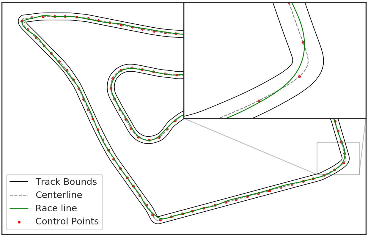
Figure 2: Race line compared to original center line of the track and control points

With this experimental setup, we design the following experiments. In Section IV-B we compare the convergence performance, stability of optimization and computation budget requirements for different optimizers. In Section IV-C we compare the effect of choosing different hyper-parameters on the performance of different optimizers. In Section IV-D we show the optimization framework’s performance in different environments and when different components are used in the autonomous system. In Section IV-E we show that it is crucial to use domain knowledge when creating initial conditions for the optimization search and it is beneficial to set up interpolation strategies to cut down the computation time in the search. In Section IV-F we perform sensitivity analysis around the solution found by the optimization. Lastly, in Section IV-G we compare the solutions found by our method with another optimization method that aims to lower a race car’s lap time on track. All optimized parameters for each experiment can be found in Tables VII and VIII.

IV-B Comparison of optimizer

The objective of this experiment is to compare the convergence performance and computational budget requirement for different optimizers. The race track, controller type for the vehicle and total computation budget are kept the same, with the optimizer used as the only difference between runs. We compare the performance of the following optimizers: 1. CMA 2. Differential Evolution (DE) with two points cross over 3. Differential Evolution with noisy recommendation 4. Particle Swarm Optimization 5. 1+1 Evolutionary algorithm 6. Random Search. We use a total of 9600 simulations for each run as the computation budget. We also use the default race track Spielberg and the default low level controller Pure Pursuit [47].

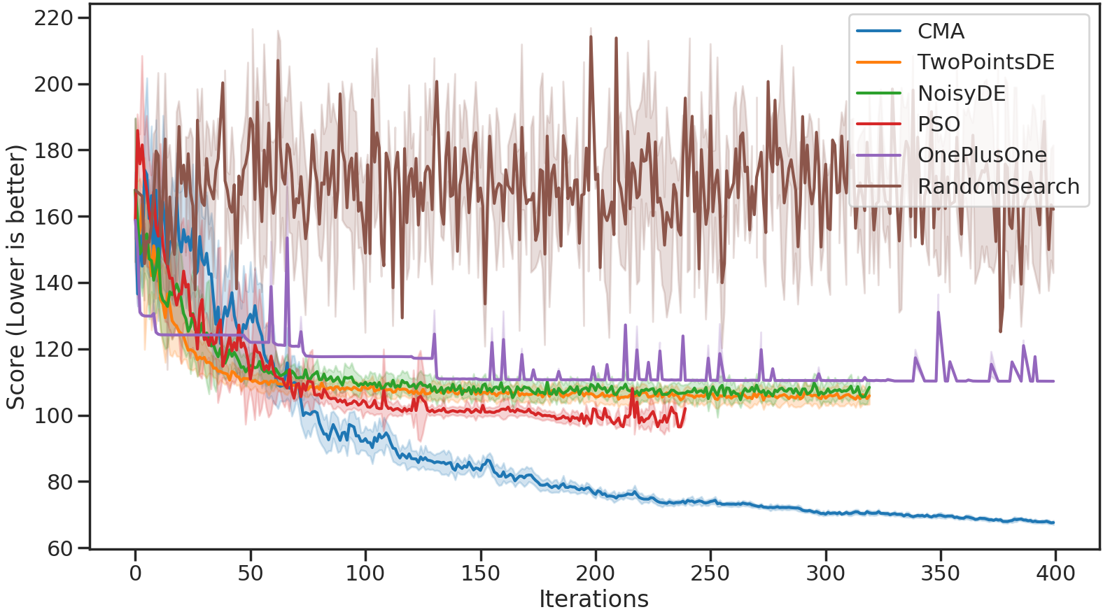
Figure 3: Convergence performance and computational budget requirement of different optimizers

We show the results of this experiment in Figure 3 as history of average lap times and standard deviation in each iteration. The Random Search optimizer performs random sampling in the search space without any search direction. We use this optimizer as the baseline for comparison. As shown in the figure, all other candidate optimizers except for the Random Search baseline shows convergent behavior and clear minimization of the objective value. Specifically, we see most of the optimizers converge to the 95 to 115 seconds range and CMA performs the best with the lowest objective value found at 66.69 seconds for 2 laps.

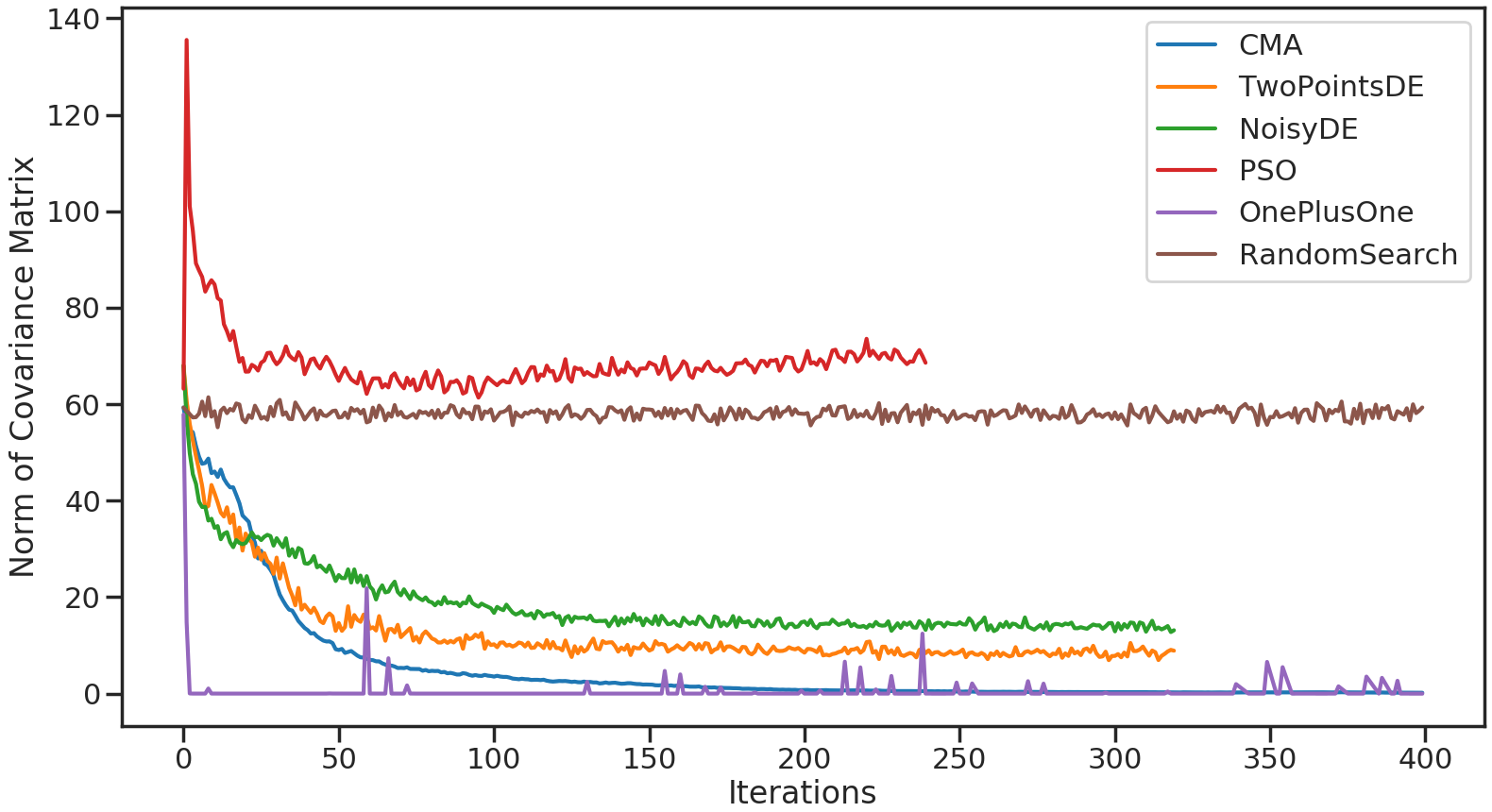
Figure 4: Progress of norm of covariance matrix of different optimizers

We also show the convergence of different algorithms as progress of the norm of covariance matrices of the batch of candidates in each iteration for different optimizers. As a baseline, we again see no convergent behavior for Random Search, since the norm of the covariance matrix remains mostly constant throughout the all iterations. For CMA and (1+1), the difference between candidates in a generation vanishes and all individuals converge to a single point. For both optimizers using DE, we see that the population has converged, but not to a single candidate, which is the reason we see non zero norms. And for PSO, the candidates stayed very diverse, even more spread out than the Random Search generations.

We infer that the good performance of CMA on this problem is due to the exploit-explore nature of the algorithm. For CMA, the populations are not confined within the vicinity of the original sampled population. For example, DE recombines genomes in the previous population, which means this operation in nature is an averaging between candidate instances in the optimization. While CMA changes the sampling strategy by modeling the spread of the candidates with a Gaussian distribution. With a larger covariance, the distribution is able to explore outside the range defined by the original sampled candidates. This is also why we see an increase in the covariance between candidates before we see a decrease.

IV-C Comparison of hyperparameters

Next, we explore different settings used by optimizers and study the effect of changing parameters in certain optimizers. We first experiment with different population sizes used for different optimizers, while keeping the total computation budget the same. CMA uses a default population size of 24 in our experiment to match the number of workers used in parallel simulation. We also experiment with population sizes 6, 12, 48 and 96. We show the average lap time and standard deviation in each generation in Figure 5 and the best lap time after all computation budget is exhausted in Table II.

Population Size	Best Lap time
6	69.65
12	73.71
24	66.69
48	67.9
96	73.78

TABLE II: Best lap time for CMA using different population sizes.

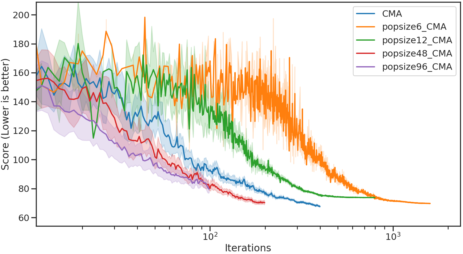
Figure 5: Progression of lap time with differnt population size used for CMA

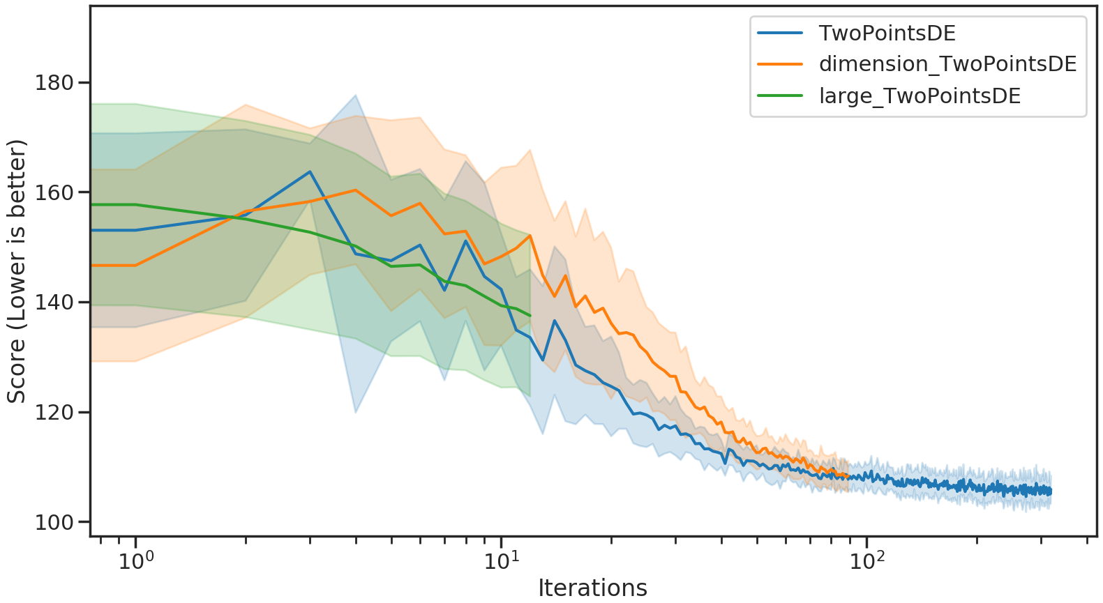
Figure 11: Progression of lap time with different population size used for TwoPointsDE

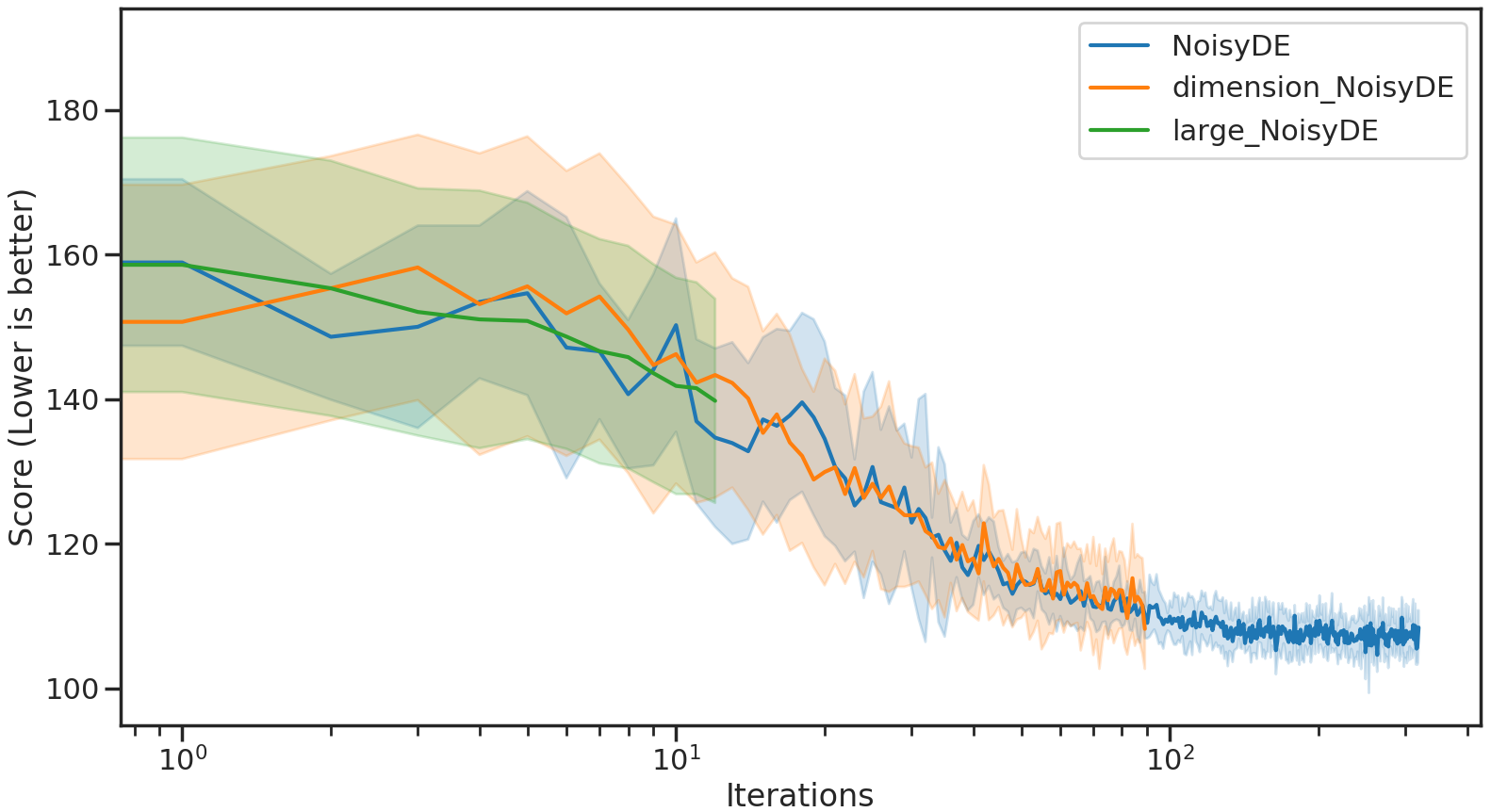
Figure 12: Progression of lap time with different population size used for NoisyDE

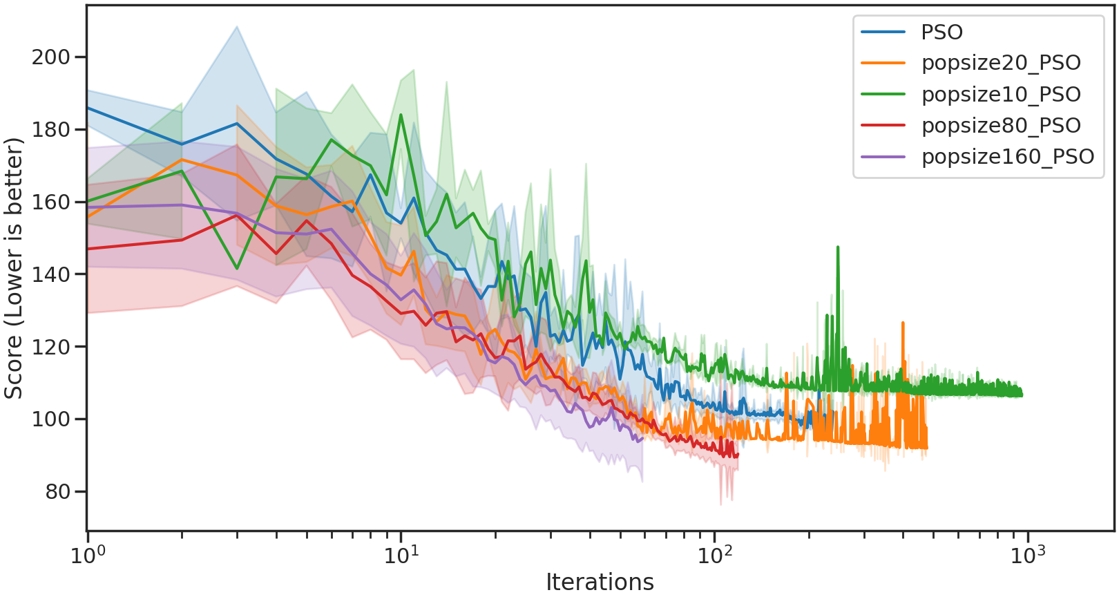
Figure 13: Progression of lap time with different population size used for PSO

We see the best lap time was achieved using the default population size of 24, with other settings also finding competitive solutions but worse than using the hyperparameter determined by the default heuristics. We also performed the sane analysis on the two DE based optimization and PSO. The results we see are similar and we show them in Figures 11, 12, and 13 in the Appendix.

IV-D Generalization of Environment and Autonomy Component

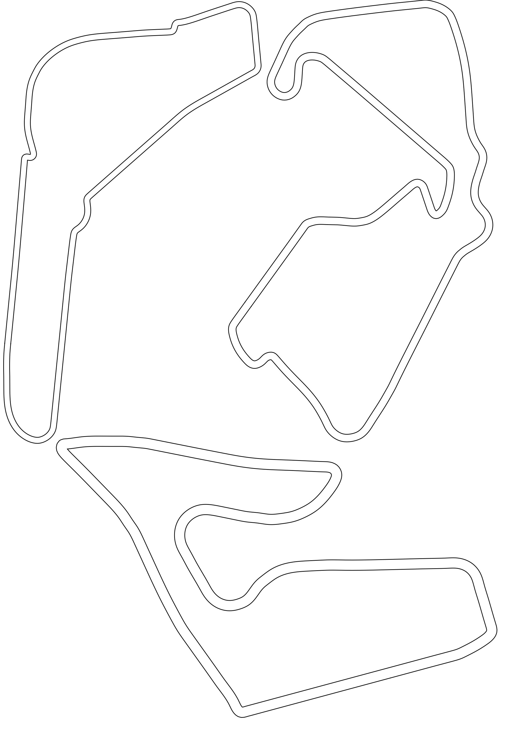
Figure 14: Race track used as environments for experiments. Top Left: Monza, Top Right: Silverstone, Bottom: Spielberg.

To display that our proposed framework is able to generalize to different systems and different operating environments, we perform the same optimization using the default setting of CMA on two more different race tracks and with different control strategies. All three race tracks have unique track layouts displayed in Figure 14 in the Appendix. The default race track Spielberg is a combination track composed of equal parts straights, sweeper curves and hairpins. While Silverstone is a more curve-heavy race track featuring sweep curves, hairpins and chicanes. Finally, Monza is a high speed race track with mostly straights and three chicanes. The resulting best lap time for each map is shown in Table III, and the progression of lap time for each map is shown in Figure 6. It is clear that the convergent behavior of the optimization shows across different system operating environments.

Race Track	Best Lap time
Spielberg	66.69
Silver Stone	89.56
Monza	113.04

TABLE III: Best lap time for CMA with Pure Pursuit on different race tracks.

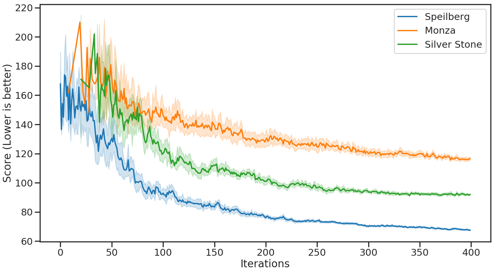
Figure 6: Progression of lap times with CMA on different race tracks.

We also experiment with using different autonomy components that fundamentally changes the behavior of the system. We drive the car with three different path tracking controllers: Pure Pursuit [47], the Stanley controller [48], and a Linear Quadratic Regulator (LQR). Both Pure Pursuit and the Stanley controller are geometric path trackers whereas LQR is an iterative optimization based method. Therefore all three controllers have different sets of parameters to be optimized. We showed the result of the three different controllers successfully being optimized in Figure 7. The best solution found by the different controllers are shown in Table IV.

Controller	Best Lap time
Pure Pursuit	66.69
Stanley	92.13
LQR	62.18

TABLE IV: Best lap time with different tuned controllers on Spielberg.

We see that LQR is able to achieve the best result, improving the solution found by using Pure Pursuit by almost five seconds, while Stanley struggled to find a fast solution, but still successfully converged to a solution. This also shows that the pipeline generalizes to systems with different components. The optimized parameters for the three different controllers are shown in Table VII in the Appendix.

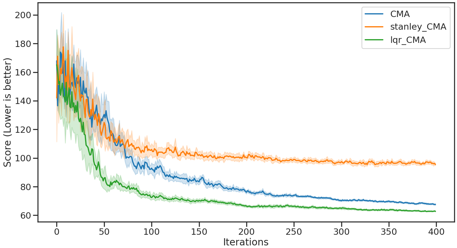
Figure 7: Progression of lap times with different path tracking controller

IV-E Interpolation the search space and changing initial conditions

We experiment with changing the initial condition for where the search starts and the constraints on parameters to show the importance of human domain knowledge in bounding the search so that it finds a valid solution easier. We experiment with the default setting using the Spielberg map and the Pure Pursuit controller, while relaxing some of the constrains we impose on the bounds of the variable parameters. We showed the different bounds in Table V. With these few constraint relaxation, the optimizer was not able to find a single solution that’s able to complete two laps on track without collision with the same computation budget of 9600 simulations.

Parameter	Original		Relaxed
	Lower	Upper	Lower	Upper
Mass (kg)	3.0	4.0	1.0	10.0
CoG to Front (m)	0.147	0.170	0.001	0.3
Lowest Velocity (m/s)	0.5	2.0	0.5	10.0
Highest Velocity (m/s)	6.0	15.0	10.0	20.0
Lookahead Distance (m)	0.2	2.0	0.2	10.0

TABLE V: Bounds for parameters on original and relaxed constraints.

IV-F Sensitivity around found solutions

We examine the points around the found solution of CMA under the default setting. We add Gaussian noises with different standard deviation to the best found solution and run 100 experiments for each scale to find the success rate of shifted solutions being able to complete two laps. We separate the experiment into four sections where noise is added to only a portion of the found solution vector. Figure 8 shows the results when noise is added to all elements, only the control related elements, only the high level decision related elements, and the physical parameter related elements of the solution vector. As we can see in the figure, the shifted solutions for all experiments maintains between 60% to 70% success rate when the noise scale is between $10\text{e}^{-4}$ and $10\text{e}^{-2.5}$. Then when the scale increases beyond $10\text{e}^{-2.5}$, the success rate falls off rapidly and hits zero at $10\text{e}^{-1}$ for Decision and All. Meanwhile, there are falloffs for both Control and Physical but the descent is not as steep. We then conclude that the sensitivity of the found solution is highest when the parameters are related to high level decision making, and not as high when it comes to physical and control parameters.

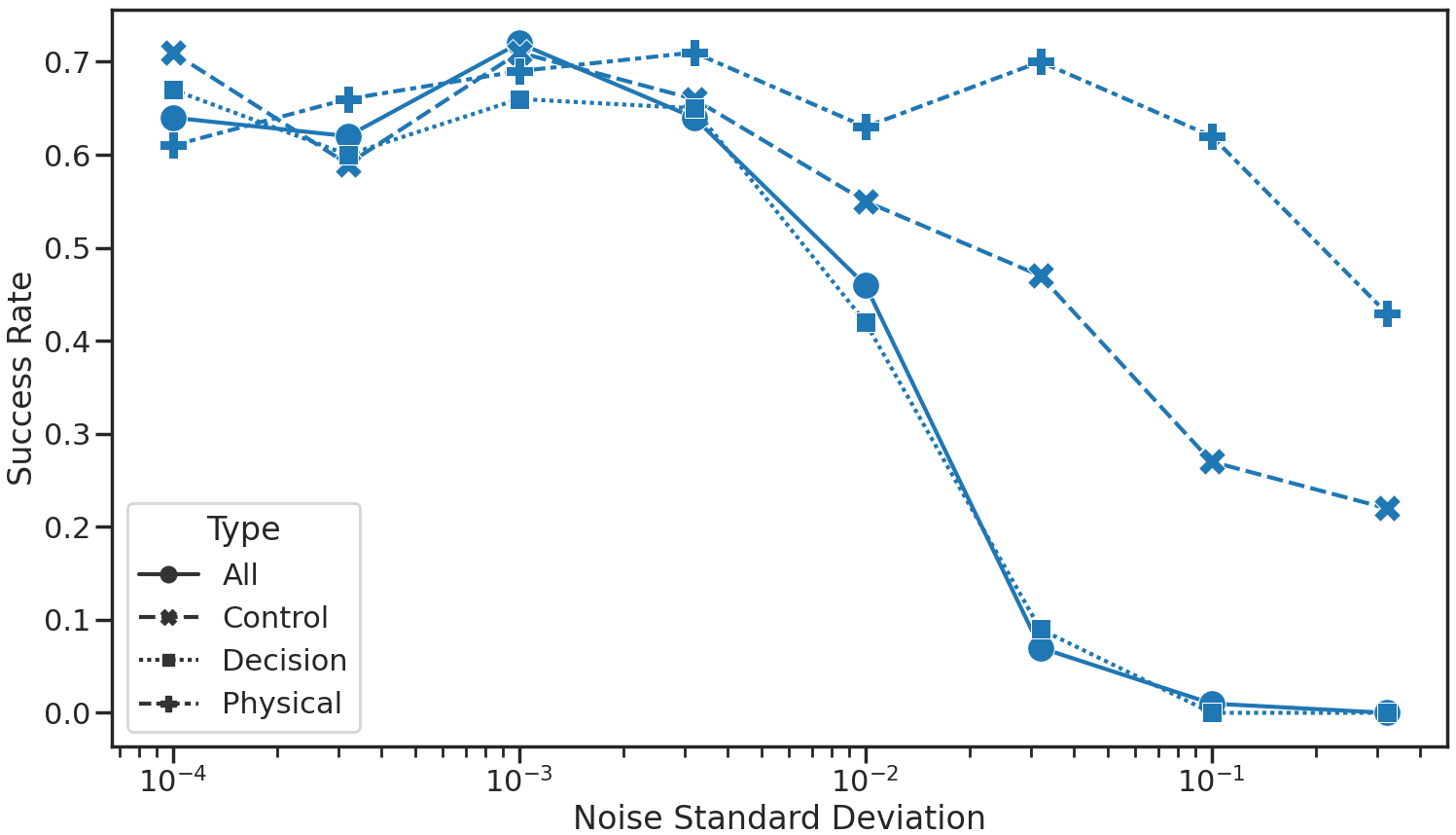
Figure 8: Success rate of solutions v.s. standard deviation of added Gaussian noise

IV-G Comparison to other methods

In this section, we closely examine the solution found by the proposed optimization framework in this paper and compare it against the solution found on the same track by a more conventional method described in Heilmeier et al.[49]. In this method, a minimum curvature path with the velocity along the path is generated by solving a QP that takes the lateral and longitudinal acceleration limits of the vehicle into account. We adopt this method to our scaled vehicle on the Spielberg track to compare with the solution found by CMA under the default setting using the LQR tracking controller. We addittionally compare the trajectory generated by tracking the path and velocity generated by Heilmeier et al. [49] using the LQR tracking controller tuned by our method.
With the same maximum allowed velocity on track, same physical vehicle parameter used, same track condition and same number of laps, our method was able to achieve 62.93 seconds for 2 complete laps. Meanwhile, the theoretical lap time from Heilmeier et al. [49] is 67.80 seconds. Using this raceline in the simulation environment with the tuned LQR controller, it achieves 69.34 seconds. Since the LQR controller cannot guarantee navigation without understeer or oversteer, the actual tracked trajectory is slower than the theoretical, minimal curvature lap time. Figure 9 shows the comparison between the trajectory produced by the two methods.

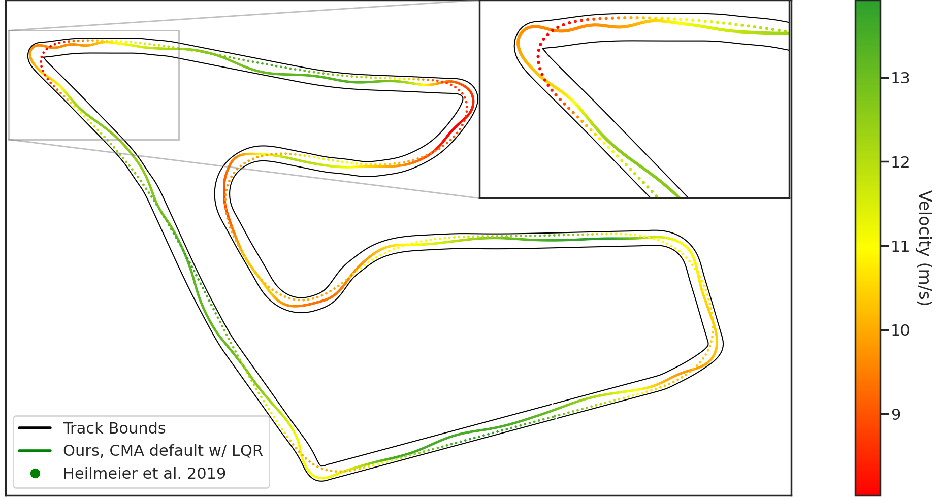
Figure 9: Trajectory comparison between our method and Heilmeier et al. where the color represents velocity and the size of the scattered dot represents the slip angle.

A notable difference between the two trajectories is that our solution does not follow the traditional conception of a fast race line. For example, as shown in the figure, our solution does not try to cut the sharp corners by using an inside line and instead drifts around the tight corner while maintaining a velocity about 2 to 3 m/s faster than a traditional race line at the corner. This results in a faster lap overall, but less room for error. Figure 10 displays an additional comparison of vehicle slip angle between our solution and the trajectory tracked using Heilmeier et al.’s race line and the tuned LQR.

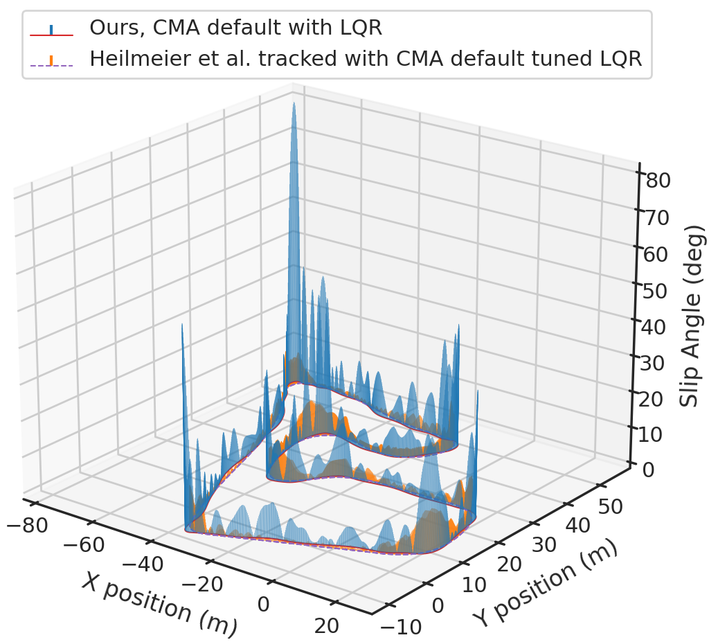
Figure 10: Trajectory of the solution found by using the LQR tracker with the default CMA optimization compared to the trajectory tracked with the same tuned LQR tracker with race line generated by Heilmeier et al.

An observation that we can make from this comparison and together with the sensitivity analysis in Section IV-F, we can conclude that our method is able to find a solution that exploits the dynamics of the simulation by finding extremely rare combinations of parameters that is able to navigate around the track with a very low lap time. At the same time, these combinations are extremely sensitive to perturbations and the slightest random noise added to the system results in crashes almost 40% of the time.

Method	Path Controller	Best Lap time
Our approach (CMA)	LQR	62.93
Heilmeier et al [49] theoretical	-	67.80
Heilmeier et al [49] practical	untuned LQR	73.64
Heilmeier et al [49] practical	tuned LQR	69.34

TABLE VI: Comparison of raceline methods on Spielberg map

V DISCUSSION

In the previous sections we provided a holistic overview of the proposed optimization framework with a rich set of experiments in the use case of autonomous racing. The results show that our optimization pipeline can indeed optimize an autonomous systems as a whole without explicitly optimizing for specific aspects of the system separately. We also showed that the pipeline generalizes to different system components (i.e. path tracking algorithms) and different system operating environments (i.e. race tracks). We observed that the proposed method is able to find solutions that achieves an improved result by exploring solutions that would not be considered by other optimization methods. It is also shown that these solutions are extremely good at the task, while being sensitive to perturbations. The proposed optimization pipeline for autonomous systems in this paper can be applied to different kinds of autonomous systems and therefore we want to provide additional guidance on how to apply our framework in the development phase of an autonomous system, focusing on 1. how to identify the proper search space for parameters; 2. techniques that accelerates and bounds the optimization; 3. selecting the correct optimizer for the problem at hand; 4. and finally, setting up the infrastructure that takes full advantage of parallelism;

In addition we will discuss the advantages and disadvantages of our method, along with further improvements that could be made.

V-A Identifying the search space

In Section II-B, we described the three sub-spaces that define the parameter set for our given problem. When identifying the search space of a new autonomous system, one should group all variable parameters into these three categories. After identifying the parameters, one should also identify the constraints on these parameters. This is mainly done by using experts in these fields that have worked in this area before. For example by developing an autonomous vehicle a vehicle width of 5m may be good for the optimization to solve design issues but is impractical considering the width constraint of street lanes.

V-B Techniques to accelerate and bound the search

1. It might be counter-intuitive to tighten the constraints in an optimization problem so that a solution can be found easier. Since gradient free optimizations are sampling based, tightening the constraints actually shrinks the search space for the algorithm and a solution within the range will be found faster. As shown in Section IV-E, having a tighter restriction on the range of values for parameters helps the optimization find valid solutions. Again, the usage of human experts in these fields are encouraged to chose the bounds of the values based on their knowledge of the system. For example, the mass and the distance from center of gravity to front axle are both based on realistic values that’s possible to achieve on the physical vehicle.

2. In addition it is important to select parameters for the optimization that have an impact on the performance of the system. For example the mass of the system is more important to the overall acceleration of the vehicle than its CoG. By having a rough idea of the sensitivity of the parameters on the whole autonomous system, it’s easier to identify the more impactful parameters and possibly easier to speed up the optimization.

V-C Selecting the right optimizer

The selection of the right optimizer that’s suitable for the problem is critical to the success of the optimization. For example, in our autonomous racing use case, the search space for parameters is large, the rollouts of each evaluation is fast, and easily parallelized, thus CMA is an excellent choice for these type of problems since it’s explore-exploit scheme is able to explore a wide range of solutions in the search space with a high number of evaluations.

If the simulation of an autonomous system is slow and inefficient, an efficient search algorithm that is able to yield improved solutions with a low number of evaluations such as OnePlusOne should be chosen as the optimizer.

Lastly, if multiple solutions that are unique is required, then such as PSO should be chosen. Although the solutions did not converge to the best possible, it was able to find improved combination of parameters that are still diverse in the given computation budget.

V-D Software infrastructure to support the optimization

Our optimization scheme takes advantage of parallelism due to the batched nature of evaluations required by the optimizers. A MapReduce [45] pattern in the software architecture is recommended for efficient evaluations. The proposed software architecture will be made available online.

V-E Advantages and Disadvantages of the proposed optimization pipeline

The advantage of the proposed pipeline is the holistic view on optimization of an autonomous system. By not restricting what explicit parameters are allowed in the formulation, both hardware and software components can be optimized at the same time. The optimization space as well as the objective function is defined by a handful of parameters and can therefore be applied to different use cases. By using lightweight simulator environments and low overhead for parallelization and optimization, we achieve efficient computation times on consumer computation hardware. For example, with 9600 evaluations, the CMA experiment with Pure Pursuit on Spielberg takes around 25 minutes on a Ryzen 5900X with no GPU requirements. The usage of HPC hardware where more parallel workers can be spawned would speed up the optimization but is not necessary. The pipeline also provides flexibility in terms of what the desired solutions have characteristically. Core components can also be changed to accommodate different system characteristics.

However, we also address the shortcomings of the proposed solution. The current simulation environment we experimented with is mainly constraint for single system scenarios. An interaction with other agents or systems is not provided or planned. The approach also did not consider the discrepancy between simulation and the real system. For example, by only defining a single objective value (in our case study: lap time), a fast lap time was achieved but with a very aggressive and inoperable vehicle behavior (high side-slip angle) which would lead to an unstable vehicle behavior on the real system. Multi-objective optimization is theoretically possible with our pipeline, yet we did not perform experiments showing if the pipeline is able to provide solutions in terms of the pareto front instead of best performance on a single metric.

VI CONCLUSIONS

We introduce a gradient-free multi-domain optimization method for autonomous systems in general. The goal of this optimization method is to optimize all system parameters (hardware, software) at the same time to find the desired objective value. We detail the suitable autonomous systems that could be optimized, how to set up the optimization pipeline, and provide guidance on selecting different variants of the core components in the pipeline according to a specific autonomous system. We also validate our solution by performing a case study on an autonomous race car to show improvements in terms of lap time and compare it to conventional optimization techniques in the same field. By carrying out different experiments we provide insights in the optimization algorithms, hyperparameter tuning, and sensitivity of found solutions. Finally we showed that the proposed method outperforms other methods in the same field for the given task and system.

Future work should focus on performing more case studies using our method on additional autonomous system (e.g. UUV, UAV) with different characteristics. Experiments with combinatorial and discrete parameters should also be performed to further validate the method’s ability to handle a wide variety of parameters. Experiments should also consider multi-objective optimization where no objective can be improved without sacrificing at least one other objective. Lastly, future improvements to the method should also consider the reality gap between the simulation evaluations and physical systems.

VII Acknowledgment

We thank Matthew O’Kelly and Achin Jain during the initial conception of the problem, and Brandon McBride for assistance in development in the software stack.

Parameter	Pure Pursuit Controller	Stanley Controller	LQR
Vehicle Mass (kg)	3.9418	3.9396	3.8052
CoG to Front (m)	0.1610	0.1666	0.1562
Max. Velocity (m/s)	14.9931	11.3578	14.9926
Min. Velocity (m/s)	1.1033	1.8482	1.9779
Lookahead Distance (m)	0.8631	-	-
Controler Gain kp	-	0.0097	-
Matrix_Q(1)	-	-	0.9991
Matrix_Q(2)	-	-	0.9537
Matrix_Q(3)	-	-	0.0066
Matrix_Q(4)	-	-	0.0257
Matrix_R	-	-	0.0062
Lap time (s)	66.69	92.13	62.18

TABLE VII: Best path tracker parameters found by CMA on Spielberg.

Parameters	Comparison of Optimizers						Diff. Pop. size of CMA					Diff. Pop. Size of 2PtsDE			Diff. Pop. Size of NDE			Diff. Pop. Size of PSO					Diff. Maps
	CMA	2PtsDE	NDE	PSO	1+1	Random Search	6	12	24	48	96	30	106	735	30	106	735	10	20	40	80	160	Silverstone	Monza
Vehicle mass (kg)	3.94	3.47	3.93	3.76	3.57	3.87	3.29	3.32	3.94	3.82	3.90	3.47	3.59	3.78	3.93	3.83	3.91	3.51	3.98	3.76	3.76	3.56	3.96	3.94
CoG to Front (m)	0.16	0.15	0.17	0.15	0.17	0.16	0.15	0.16	0.16	0.15	0.15	0.15	0.16	0.16	0.17	0.16	0.16	0.16	0.16	0.15	0.17	0.16	0.15	0.15
Max. Velocity (m/s)	14.99	9.78	9.65	10.62	10.83	9.32	15.00	13.92	14.99	14.89	14.10	9.78	9.93	9.79	9.65	10.73	10.35	10.22	10.63	10.62	11.24	11.88	14.82	10.42
Min. Velocity (m/s)	1.10	1.47	1.99	1.47	0.60	1.93	1.37	1.22	1.10	1.55	1.73	1.47	1.31	1.92	1.99	0.96	1.90	1.21	1.99	1.47	1.94	1.59	1.90	1.67
Lookahead Distance (m)	1.75	1.00	1.00	1.00	1.17	2.00	1.66	1.43	1.75	1.86	1.82	1.00	1.19	1.19	1.00	1.87	1.71	0.94	1.17	1.01	1.12	1.46	1.46	1.09
Laptime (s)	66.69	100.20	99.85	96.39	110.21	115.29	69.65	73.71	66.69	67.90	73.78	100.20	101.09	108.63	99.85	98.52	106.47	106.20	91.86	96.39	86.97	85.91	89.56	113.04

TABLE VIII: Overview of optimized parameters from different experiments using Pure Pursuit

Hongrui Zheng received his B.S. degrees in Mechanical Engineering and Computer Science from Georgia Institute of Technology, and his M.S. degree in Robotics from University of Pennsylvania. He is currently a Ph.D. candidate at University of Pennsylvania. His research focuses on building the tools and theoretical foundations necessary to scale design, testing, and optimization of safe-autonomous systems.

Johannes Betz is a postdoctoral researcher at the University of Pennsylvania where he is am working at the mLab: Real-Time and Embedded Systems Lab. His research is focusing on a holistic software development for autonomous systems with extreme motions at the dynamic limits in extreme and unknown environments. By using modern algorithms from the field of artificial intelligence he is trying to develop new and advanced methods and intelligent algorithms. Based on his additional studies in philosophy he extends current path and behavior planners for autonomous systems with ethical theories.

Rahul Mangharam received his Ph.D. in Electrical and Computer Engineering from Carnegie Mellon University where he also received his MS and BS. He is an Associate Professor in the Department of Electrical and Systems Engineering at the University of Pennsylvania. He is a founding member of the PRECISE Center and directs the Safe Autonomous Systems Lab at Penn. His research is at the intersection of formal methods, machine learning and control for medical devices, energy efficient buildings, and autonomous systems.

References

- [1] S. D. Pendleton, H. Andersen, X. Du, X. Shen, M. Meghjani, Y. H. Eng, D. Rus, and M. H. Ang, “Perception, planning, control, and coordination for autonomous vehicles,” Machines, vol. 5, no. 1, 2017. [Online]. Available: https://www.mdpi.com/2075-1702/5/1/6
- [2] N. Hansen and A. Ostermeier, “Completely derandomized self-adaptation in evolution strategies,” Evolutionary computation, vol. 9, no. 2, pp. 159–195, 2001.
- [3] K. V. Price, “Differential evolution,” in Handbook of optimization. Springer, 2013, pp. 187–214.
- [4] J. Kennedy and R. Eberhart, “Particle swarm optimization,” in Proceedings of ICNN’95-international conference on neural networks, vol. 4. IEEE, 1995, pp. 1942–1948.
- [5] Y. Shi and R. Eberhart, “A modified particle swarm optimizer,” in 1998 IEEE international conference on evolutionary computation proceedings. IEEE world congress on computational intelligence (Cat. No. 98TH8360). IEEE, 1998, pp. 69–73.
- [6] M. Styner, C. Brechbuhler, G. Szckely, and G. Gerig, “Parametric estimate of intensity inhomogeneities applied to mri,” IEEE transactions on medical imaging, vol. 19, no. 3, pp. 153–165, 2000.
- [7] M. O'Kelly, H. Zheng, A. Jain, J. Auckley, K. Luong, and R. Mangharam, “TUNERCAR: A superoptimization toolchain for autonomous racing,” in 2020 IEEE International Conference on Robotics and Automation (ICRA). IEEE, May 2020. [Online]. Available: https://doi.org/10.1109/icra40945.2020.9197080
- [8] H. M. Buini, S. Peter, and T. Givargis, “Including variability of physical models into the design automation of cyber-physical systems,” in Proceedings of the 52nd Annual Design Automation Conference, ser. DAC ’15. New York, NY, USA: Association for Computing Machinery, 2015. [Online]. Available: https://doi.org/10.1145/2744769.2744857
- [9] N. Mühleis, M. Glaß, L. Zhang, and J. Teich, “A co-simulation approach for control performance analysis during design space exploration of cyber-physical systems,” SIGBED Rev., vol. 8, no. 2, p. 23–26, Jun. 2011. [Online]. Available: https://doi.org/10.1145/2000367.2000372
- [10] T. Campos, J. P. Inala, A. Solar-Lezama, and H. Kress-Gazit, “Task-based design of ad-hoc modular manipulators,” in 2019 International Conference on Robotics and Automation (ICRA). IEEE, 2019, pp. 6058–6064.
- [11] Y. Vanommeslaeghe, J. Denil, J. D. Viaene, D. Ceulemans, S. Derammelaere, and P. D. Meulenaere, “Leveraging domain knowledge for the efficient design-space exploration of advanced cyber-physical systems,” in 2019 22nd Euromicro Conference on Digital System Design (DSD). IEEE, Aug. 2019. [Online]. Available: https://doi.org/10.1109/dsd.2019.00058
- [12] J. Bradley and E. Atkins, “Optimization and control of cyber-physical vehicle systems,” Sensors, vol. 15, no. 9, pp. 23 020–23 049, Sep. 2015. [Online]. Available: https://doi.org/10.3390/s150923020
- [13] Z. Lattmann, A. Nagel, J. Scott, K. Smyth, C. vanBuskirk, J. Porter, S. Neema, T. Bapty, J. Sztipanovits, J. Ceisel, and D. Mavris, “Towards automated evaluation of vehicle dynamics in system-level designs,” in Volume 2: 32nd Computers and Information in Engineering Conference, Parts A and B. American Society of Mechanical Engineers, Aug. 2012. [Online]. Available: https://doi.org/10.1115/detc2012-71378
- [14] S.-C. Lin, Y. Zhang, C.-H. Hsu, M. Skach, M. E. Haque, L. Tang, and J. Mars, “The architectural implications of autonomous driving,” ACM SIGPLAN Notices, vol. 53, no. 2, pp. 751–766, Nov. 2018. [Online]. Available: https://doi.org/10.1145/3296957.3173191
- [15] A. Collin, A. Siddiqi, Y. Imanishi, E. Rebentisch, T. Tanimichi, and O. L. Weck, “Autonomous driving systems hardware and software architecture exploration: optimizing latency and cost under safety constraints,” Systems Engineering, vol. 23, no. 3, pp. 327–337, Dec. 2019. [Online]. Available: https://doi.org/10.1002/sys.21528
- [16] R. Toscano, “A simple robust PI/PID controller design via numerical optimization approach,” Journal of Process Control, vol. 15, no. 1, pp. 81–88, Feb. 2005. [Online]. Available: https://doi.org/10.1016/j.jprocont.2004.03.005
- [17] N. Killingsworth and M. Krstic, “PID tuning using extremum seeking: online, model-free performance optimization,” IEEE Control Systems, vol. 26, no. 1, pp. 70–79, Feb. 2006. [Online]. Available: https://doi.org/10.1109/mcs.2006.1580155
- [18] T. S. Kim, J. C. Na, and K. J. Kim, “Optimization of an autonomous car controller using a self-adaptive evolutionary strategy,” International Journal of Advanced Robotic Systems, vol. 9, no. 3, p. 73, Jan. 2012. [Online]. Available: https://doi.org/10.5772/50848
- [19] O. Castillo, R. Martínez-Marroquín, P. Melin, F. Valdez, and J. Soria, “Comparative study of bio-inspired algorithms applied to the optimization of type-1 and type-2 fuzzy controllers for an autonomous mobile robot,” Information Sciences, vol. 192, pp. 19–38, Jun. 2012. [Online]. Available: https://doi.org/10.1016/j.ins.2010.02.022
- [20] W. Ma, Y. Pang, C. Jiang, and X. Du, “Research on the optimization of PID control of remotely operated underwater vehicle,” in 2011 International Conference on Computer Science and Service System (CSSS). IEEE, Jun. 2011. [Online]. Available: https://doi.org/10.1109/csss.2011.5974874
- [21] S. Dai, J. Hite, T. Masuda, Y. Kashiba, N. Arechiga, S. Shiraishi, S. Eisele, J. Scott, and T. Bapty, “Control parameter optimization for autonomous vehicle software using virtual prototyping,” in 2017 IEEE International Symposium on Software Reliability Engineering Workshops (ISSREW). IEEE, Oct. 2017. [Online]. Available: https://doi.org/10.1109/issrew.2017.15
- [22] J. E. Naranjo, F. Serradilla, and F. Nashashibi, “Speed control optimization for autonomous vehicles with metaheuristics,” Electronics, vol. 9, no. 4, p. 551, Mar. 2020. [Online]. Available: https://doi.org/10.3390/electronics9040551
- [23] D. Nguyen-Tuong and J. Peters, “Local gaussian processes regression for real-time model-based robot control,” in IROS 2008, Max-Planck-Gesellschaft. Piscataway, NJ, USA: IEEE Service Center, Sep. 2008, pp. 380–385.
- [24] A. Wischnewski, J. Betz, and B. Lohmann, “Real-time learning of non-gaussian uncertainty models for autonomous racing,” in 2020 59th IEEE Conference on Decision and Control (CDC). IEEE, Dec. 2020. [Online]. Available: https://doi.org/10.1109/cdc42340.2020.9304230
- [25] J. Kabzan, L. Hewing, A. Liniger, and M. N. Zeilinger, “Learning-based model predictive control for autonomous racing,” IEEE Robotics and Automation Letters, vol. 4, no. 4, pp. 3363–3370, Oct. 2019. [Online]. Available: https://doi.org/10.1109/lra.2019.2926677
- [26] D. Belter and P. Skrzypczyński, “Population-based methods for identification and optimization of a walking robot model,” in Robot Motion and Control 2009, K. R. Kozłowski, Ed. London: Springer London, 2009, pp. 185–195.
- [27] M. Jaderberg, V. Dalibard, S. Osindero, W. M. Czarnecki, J. Donahue, A. Razavi, O. Vinyals, T. Green, I. Dunning, K. Simonyan et al., “Population based training of neural networks,” arXiv preprint arXiv:1711.09846, 2017.
- [28] E. Conti, V. Madhavan, F. P. Such, J. Lehman, K. O. Stanley, and J. Clune, “Improving exploration in evolution strategies for deep reinforcement learning via a population of novelty-seeking agents,” 2018.
- [29] S. Khadka and K. Tumer, “Evolutionary reinforcement learning,” CoRR, vol. abs/1805.07917, 2018. [Online]. Available: http://arxiv.org/abs/1805.07917
- [30] D. Ha and J. Schmidhuber, “Recurrent world models facilitate policy evolution,” in Advances in Neural Information Processing Systems 31. Curran Associates, Inc., 2018, pp. 2451–2463, https://worldmodels.github.io. [Online]. Available: https://papers.nips.cc/paper/7512-recurrent-world-models-facilitate-policy-evolution
- [31] W. Schwarting, T. Seyde, I. Gilitschenski, L. Liebenwein, R. Sander, S. Karaman, and D. Rus, “Deep latent competition: Learning to race using visual control policies in latent space,” 2021.
- [32] A. Amini, I. Gilitschenski, J. Phillips, J. Moseyko, R. Banerjee, S. Karaman, and D. Rus, “Learning robust control policies for end-to-end autonomous driving from data-driven simulation,” IEEE Robotics and Automation Letters, vol. 5, no. 2, pp. 1143–1150, Apr. 2020. [Online]. Available: https://doi.org/10.1109/lra.2020.2966414
- [33] R. Martinez-Cantin, “Funneled bayesian optimization for design, tuning and control of autonomous systems,” IEEE Transactions on Cybernetics, vol. 49, no. 4, pp. 1489–1500, Apr. 2019. [Online]. Available: https://doi.org/10.1109/tcyb.2018.2805695
- [34] Y. Song, Y.-b. Li, C.-h. Li, and G.-f. Zhang, “An efficient initialization approach of q-learning for mobile robots,” International Journal of Control, Automation and Systems, vol. 10, no. 1, pp. 166–172, 2012.
- [35] E. Schkufza, R. Sharma, and A. Aiken, “Stochastic superoptimization,” in ACM SIGPLAN Notices, vol. 48, no. 4. ACM, 2013, pp. 305–316.
- [36] H. Massalin, “Superoptimizer: a look at the smallest program,” in ACM SIGARCH Computer Architecture News, vol. 15, no. 5. IEEE Computer Society Press, 1987, pp. 122–126.
- [37] A. Solar-Lezama, “Program sketching,” International Journal on Software Tools for Technology Transfer, vol. 15, no. 5-6, pp. 475–495, 2013.
- [38] P. Liang, M. I. Jordan, and D. Klein, “Learning programs: A hierarchical bayesian approach,” in Proceedings of the 27th International Conference on Machine Learning (ICML-10), 2010, pp. 639–646.
- [39] C. A. Lattner, “Llvm: An infrastructure for multi-stage optimization,” Ph.D. dissertation, University of Illinois at Urbana-Champaign, 2002.
- [40] N. Vasilache, O. Zinenko, T. Theodoridis, P. Goyal, Z. DeVito, W. S. Moses, S. Verdoolaege, A. Adams, and A. Cohen, “Tensor comprehensions: Framework-agnostic high-performance machine learning abstractions,” arXiv preprint arXiv:1802.04730, 2018.
- [41] J. Ragan-Kelley, C. Barnes, A. Adams, S. Paris, F. Durand, and S. Amarasinghe, “Halide: a language and compiler for optimizing parallelism, locality, and recomputation in image processing pipelines,” in Acm Sigplan Notices, vol. 48, no. 6. ACM, 2013, pp. 519–530.
- [42] M. O’Kelly, H. Zheng, D. Karthik, and R. Mangharam, “F1tenth: An open-source evaluation environment for continuous control and reinforcement learning,” in NeurIPS 2019 Competition and Demonstration Track. PMLR, 2020, pp. 77–89.
- [43] M. Althoff, M. Koschi, and S. Manzinger, “Commonroad: Composable benchmarks for motion planning on roads,” in 2017 IEEE Intelligent Vehicles Symposium (IV). IEEE, 2017, pp. 719–726.
- [44] P. Moritz, R. Nishihara, S. Wang, A. Tumanov, R. Liaw, E. Liang, M. Elibol, Z. Yang, W. Paul, M. I. Jordan et al., “Ray: A distributed framework for emerging AI applications,” in 13th USENIX Symposium on Operating Systems Design and Implementation (OSDI 18), 2018, pp. 561–577.
- [45] J. Dean and S. Ghemawat, “Mapreduce: simplified data processing on large clusters,” Communications of the ACM, vol. 51, no. 1, pp. 107–113, 2008.
- [46] J. Rapin and O. Teytaud, “Nevergrad - A gradient-free optimization platform,” https://GitHub.com/FacebookResearch/Nevergrad, 2018.
- [47] R. C. Coulter, “Implementation of the pure pursuit path tracking algorithm,” Carnegie-Mellon UNIV Pittsburgh PA Robotics INST, Tech. Rep., 1992.
- [48] S. Thrun, M. Montemerlo, H. Dahlkamp, D. Stavens, A. Aron, J. Diebel, P. Fong, J. Gale, M. Halpenny, G. Hoffmann et al., “Stanley: The robot that won the darpa grand challenge,” Journal of field Robotics, vol. 23, no. 9, pp. 661–692, 2006.
- [49] A. Heilmeier, A. Wischnewski, L. Hermansdorfer, J. Betz, M. Lienkamp, and B. Lohmann, “Minimum curvature trajectory planning and control for an autonomous race car,” Vehicle System Dynamics, 2019.