Towards Unifying Logical Entailment and Statistical Estimation

Abstract

This paper gives a generative model of the interpretation of formal logic for data-driven logical reasoning. The key idea is to represent the interpretation as likelihood of a formula being true given a model of formal logic. Using the likelihood, Bayes’ theorem gives the posterior of the model being the case given the formula. The posterior represents an inverse interpretation of formal logic that seeks models making the formula true. The likelihood and posterior cause Bayesian learning that gives the probability of the conclusion being true in the models where all the premises are true. This paper looks at statistical and logical properties of the Bayesian learning. It is shown that the generative model is a unified theory of several different types of reasoning in logic and statistics.

1 Introduction

Thanks to big data and computational power available today, Bayesian statistics plays an important role in various fields such as neuroscience, cognitive science and artificial intelligence (AI). Bayesian brain hypothesis Knill and Pouget (2004), free-energy principle Friston (2010) and predictive coding Hohwy et al. (2008) argue that probabilistic reasoning using Bayes’ theorem or its approximation explains some higher-order cognitive functions of the cerebral cortex such as perception, action and learning. The common idea is that the brain is a generative model that actively predicts and perceives the world using the belief of states of the world. Bayes’ theorem here defines how sensory inputs such as sight, sound, smell, taste and touch update the belief.

Formal logic concerns the laws of human rational thought. The Bayesian brain hypothesis would therefore result in another hypothesis that there is a Bayesian algorithm and data-structure for logical reasoning. This hypothesis is important for the following reasons. First, it has a potential to cause a mathematical model to explain how the human brain performs logical reasoning. Second, the existence of such a model supports the Bayesian brain hypothesis in terms of formal logic. Third, such a model gives a way to critically assess the existing formalisms of logical reasoning. Nevertheless, few research has focused on reformulating logical reasoning in terms of Bayesian perspectives. Bayesian networks Pearl (1988), probabilistic relational models (PRM) Friedman et al. (1996), probabilistic logic programming (PLP) Sato (1995) and Markov logic networks (MLN) Richardson and Domingos (2006) are a few exceptions intrinsically relating to Bayesian inference. However, none of them aims to model the process by which data about states of the world generate models of formal logic and then the models generate the truth values of logical formulae. Such a model should give a unified way to deal with the tasks of the statistics and logic shown in Figure 1. This is an important problem because various challenging AI problems such as grounding, frame problems, knowledge acquisition bottleneck, commonsense reasoning and contextual adaptation, come from their disconnection.

Formal logic considers an interpretation on each model (denoted by $m$), which represents a state of the world. The interpretation is a function that maps each formula (denoted by $\alpha$) to a truth value, which represents knowledge of the world. Our idea is to give a generative model of the interpretation and use it to probabilistically generate knowledge from data about states of the world. The most basic theoretical idea is to represent the interpretation as likelihood $p(\alpha|m)$. Using the likelihood, Bayes’ theorem gives posterior $p(m|\alpha)$, which represents an inverse interpretation that gives the probability that the model making formula $\alpha$ true is $m$. The likelihood and posterior cause Bayesian learning $p(\alpha|\beta)=\sum_{m}p(\alpha|m)p(m|\beta)$, which gives the probability of the formula $\alpha$ being true in the models where the formula $\beta$ is true. This paper studies statistical and logical properties of the Bayesian learning.

This paper is organised as follows. Section 2 introduces a generative model for logical consequence relations. Section 3 shows logical and statistical correctness of the generative model. Section 4 concludes with a discussion of limitations and future work.

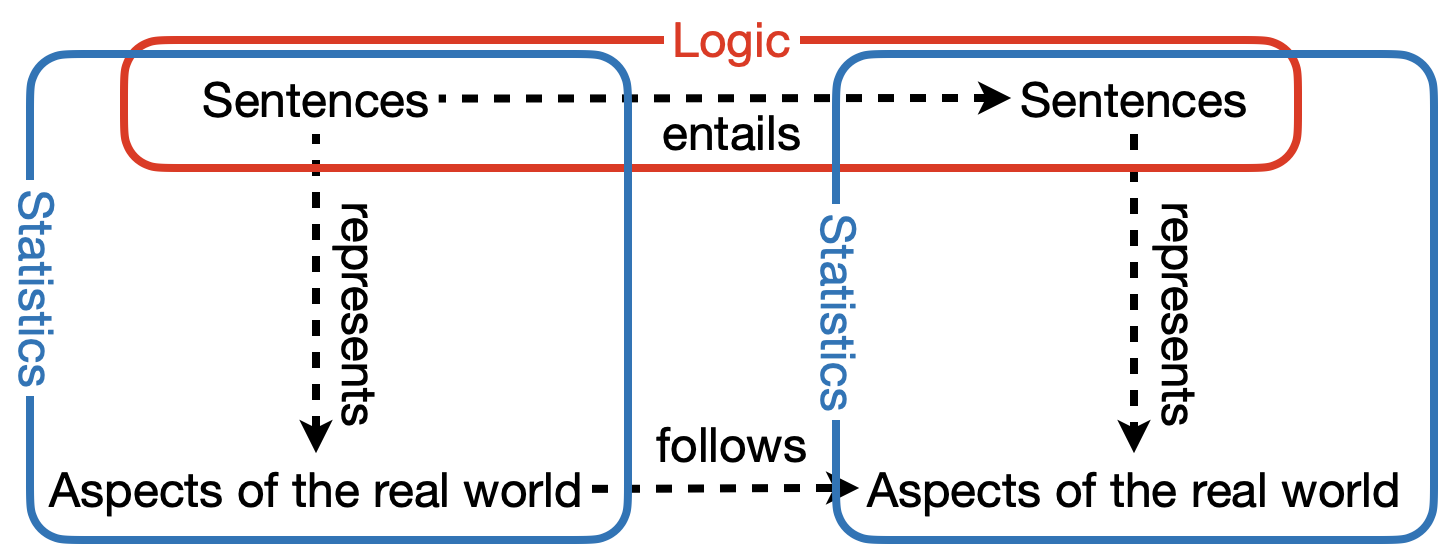
Figure 1: Logic concerns if sentences follow logically from other whereas statistics concerns if they reflect aspects of the real world.

2 Method

Let ${\cal D}=\{d_{1},d_{2},...,d_{K}\}$ be a multiset of data about states of the world. $D$ is a random variable whose realisations are data in ${\cal D}$. For all data $d_{k}\in{\cal D}$, we define the probability of $d_{k}$, as follows.

$$p(D=d_{k})=\frac{1}{K}$$

$L$ represents a propositional or first-order language. For the sake of simplicity, we assume no function symbol or open formula in $L$. ${\cal M}=\{m_{1},m_{2},...,m_{N}\}$ is a set of models in formal logic. ${\cal D}$ is assumed to be complete with respect to ${\cal M}$, and thus each data in ${\cal D}$ belongs to a single model in ${\cal M}$. $m$ is a function that maps each data to such a single model. $K_{n}$ denotes the number of data that belongs to $m_{n}$, i.e., $K_{n}=|\{d_{k}\in{\cal D}|m_{n}=m(d_{k})\}|$ where $|X|$ for set $X$ denotes the cardinality of $X$. $M$ is a random variable whose realisations are models in ${\cal M}$. For all models $m_{n}\in{\cal M}$ and data $d_{k}\in{\cal D}$, we define the conditional probability of $m_{n}$ given $d_{k}$, as follows.

$$p(M=m_{n}|D=d_{k})=\begin{cases}1&\text{if }m_{n}=m(d_{k})\\ 0&\text{otherwise }\end{cases}$$

Formal logic considers an interpretation on each model. The interpretation is a function that maps each formula to a truth value, which represents knowledge of the world. We here introduce parameter $\mu\in[0,1]$ to represent the extent to which each model is taken for granted in the interpretation. Concretely, $\mu$ denotes the probability that a formula is interpreted as being true (resp. false) in a model where it is true (resp. false). $1-\mu$ is therefore the probability that a formula is interpreted as being true (resp. false) in a model where it is false (resp. true). We assume that each formula is a random variable whose realisations are 0 and 1, denoting false and true, respectively. For all models $m_{n}\in{\cal M}$ and formulae $\alpha\in L$, we define the conditional probability of each truth value of $\alpha$ given $m_{n}$, as follows.

$$p(\alpha=1|M=m_{n})=\begin{cases}\mu&\text{if }m_{n}\in\llbracket\alpha=1\rrbracket\\ 1-\mu&\text{otherwise }\end{cases}$$

$$p(\alpha=0|M=m_{n})=\begin{cases}\mu&\text{if }m_{n}\in\llbracket\alpha=0\rrbracket\\ 1-\mu&\text{otherwise }\end{cases}$$

Here, $\llbracket\alpha=1\rrbracket$ denotes the set of all models in which $\alpha$ is true, and $\llbracket\alpha=0\rrbracket$ the set of all models in which $\alpha$ is false. The above expressions can be simply written as a Bernoulli distribution with parameter $\mu\in[0,1]$, i.e.,

$$p(\alpha|M=m_{n})=\mu^{\llbracket\alpha\rrbracket_{m_{n}}}(1-\mu)^{1-\llbracket\alpha\rrbracket_{m_{n}}}.$$

Here, $\llbracket\alpha\rrbracket_{m_{n}}$ is a function such that $\llbracket\alpha\rrbracket_{m_{n}}=1$ if $m_{n}\in\llbracket\alpha\rrbracket$ and $\llbracket\alpha\rrbracket_{m_{n}}=0$ otherwise. Recall that $\alpha$ is a random variable, and thus $\llbracket\alpha\rrbracket_{m_{n}}$ is either $\llbracket\alpha=0\rrbracket_{m_{n}}$ or $\llbracket\alpha=1\rrbracket_{m_{n}}$.

In classical logic, given a model, the truth value of each formula is independently determined. In probability theory, this means that the truth values of any two formulae $\alpha_{1}$ and $\alpha_{2}$ are conditionally independent given a model $m_{n}$, i.e., $p(\alpha_{1},\alpha_{2}|M=m_{n})=p(\alpha_{1}|M=m_{n})p(\alpha_{2}|M=m_{n})$. Note that the conditional independence holds not only for atomic formulae but for compound formulae as well. Let $\Delta=\{\alpha_{1},\alpha_{2},...,\alpha_{J}\}$ be a multiset of $J$ formulae. We thus have

$$p(\Delta|M=m_{n})=\prod_{j=1}^{J}p(\alpha_{j}|M=m_{n}).$$

Thus far, we have defined $p(D)$ and $p(M|D)$ as categorical distributions and $p(\Delta|M)$ as Bernoulli distributions with parameter $\mu$. Given a value of the parameter $\mu$, they provide the full joint distribution over all of the random variables, i.e. $p(\Delta,M,D)$. We call $\{p(\Delta|M,\mu),p(M|D),p(D)\}$ a logical model. In sum, the logical model defines a data-driven interpretation by which the truth values of formulae are logically interpreted and probabilistically generated from models. The models are also probabilistically generated from data observed from the real world. The logical model meets the following important properties.

Proposition 1.

The logical model satisfies Kolmogorov’s axioms.

Proposition 2.

Let $\alpha\in L$. $p(\alpha=0)=p(\neg\alpha=1)$ holds.

In the following, we therefore replace $\alpha=0$ by $\lnot\alpha=1$ and then abbreviate $\lnot\alpha=1$ to $\lnot\alpha$. We also abbreviate $M=m_{n}$ to $m_{n}$ and $D=d_{k}$ to $d_{k}$.

Table 1: Models and data.

	$rain$	$wet$	data ${\cal D}$
$m_{1}$	$0$	$0$	$\times\times\times\times$
$m_{2}$	$0$	$1$	$\times\times$
$m_{3}$	$1$	$0$	$\times$
$m_{4}$	$1$	$1$	$\times\times\times$

Table 2: Likelihoods.

	$p(rain|M)$	$p(wet|M)$
$m_{1}$	$1-\mu$	$1-\mu$
$m_{2}$	$1-\mu$	$\mu$
$m_{3}$	$\mu$	$1-\mu$
$m_{4}$	$\mu$	$\mu$

Example 1.

Let $rain$ and $wet$ be two propositional symbols meaning ‘it is raining’ and ‘the grass is wet,’ respectively. Each row of Table 2 shows a different model, i.e., valuation. The last column shows how many data belongs to each model. Table 2 shows the likelihoods of the atomic propositions being true given a model. Given $\{p(\Delta|M,\mu=1),p(M|D),p(D)\}$, we have

$$p(rain|wet)$$

$$=\frac{\sum_{n=1}^{N}p(rain|m_{n})p(wet|m_{n})\sum_{k=1}^{K}p(m_{n}|d_{k})p(d_{k})}{\sum_{n=1}^{N}p(wet|m_{n})\sum_{k=1}^{K}p(m_{n}|d_{k})p(d_{k})}$$

$$=\frac{\sum_{n=1}^{N}p(rain|m_{n})p(wet|m_{n})\frac{K_{n}}{K}}{\sum_{n=1}^{N}p(wet|m_{n})\frac{K_{n}}{K}}$$

$$=\frac{(1-\mu)^{2}\frac{4}{10}+(1-\mu)\mu\frac{2}{10}+\mu(1-\mu)\frac{1}{10}+\mu^{2}\frac{3}{10}}{(1-\mu)\frac{4}{10}+\mu\frac{2}{10}+(1-\mu)\frac{1}{10}+\mu\frac{3}{10}}$$

$$=\frac{3}{2+3}=0.6.$$

Example 2.

Suppose that $L$ has only one 2-ary predicate symbol ‘$blames$’ and that the Herbrand universe for $L$ has only two constants $\{a,b\}$. There are four ground atoms, $\{blames(a,a),blames(a,b)$, $blames(b,a)$, $blames(b,b)\}$, which result in $2^{4}=16$ possible models. Each row of Table 3 shows a different model and the last column shows the number of data that belongs to the model. Models without data are abbreviated from the table. Given $\{p(\Delta|M,\mu=1),p(M|D),p(D)\}$, we have

$$p(\forall x~{}blames(x,a)|\exists x~{}blames(x,a))$$

$$=\frac{\sum_{n=1}^{16}\llbracket\forall x~{}blames(x,a),\exists x~{}blames(x,a)\rrbracket_{m_{n}}\frac{K_{n}}{K}}{\sum_{n=1}^{16}\llbracket\exists x~{}blames(x,a)\rrbracket_{m_{n}}\frac{K_{n}}{K}}$$

$$=\frac{K_{2}}{K_{1}+K_{2}}=\frac{3}{2+3}=0.6.$$

Table 3: Three predicate models and ten associated data.

	$blames$
	$(a,a)$	$(a,b)$	$(b,a)$	$(b,b)$	data ${\cal D}$
$m_{1}$	1	0	0	1	$\times\times$
$m_{2}$	1	1	1	0	$\times\times\times$
$m_{3}$	0	1	0	1	$\times\times\times\times\times$
other	other				no data

3 Correctness

3.1 Statistical Estimation

Fenstad Fenstad (1967) says that the probability of a formula is the sum of the probabilities of the models where the formula is true. Let $\alpha\in L$ and $m_{n}\in{\cal M}$. When $L$ has no function symbol or open formula, the first Fenstad theorem can have the following simpler form, where $m_{n}\models\alpha$ represents $m_{n}$ satisfies $\alpha$.

$$p(\alpha)=\sum_{n=1:m_{n}\models\alpha}^{N}p(m_{n})$$ (1)

When one has no prior knowledge about the probability of models, the most frequently used method to estimate $p(M)$ only from data is maximum likelihood estimation, which is given as follows.

$$p(M)=\operatorname*{arg\,max}_{\Phi}p({\cal D}|\Phi)$$

Assuming that each data is independent given $\Phi$, we have

$$p({\cal D}|\Phi)=\prod_{k=1}^{K}p(d_{k}|\Phi)$$

$$=\phi_{1}^{K_{1}}\phi_{2}^{K_{2}}\cdots\phi_{N-1}^{K_{N-1}}(1-\phi_{1}-\phi_{2}-\cdots-\phi_{N-1})^{K_{N}}.$$

$\Phi$ maximises the likelihood if and only if it maximises the log likelihood, which is given as follows.

$$L(\Phi) = K_{1}\log\phi_{1}+K_{2}\log\phi_{2}+\cdots+K_{N-1}\log\phi_{N-1}$$

$$+K_{N}\log(1-\phi_{1}-\phi_{2}-\cdots-\phi_{N-1})$$

The maximum likelihood estimate is obtained by solving the following simultaneous equations, which are obtained by differentiating the log likelihood with respect to each $\phi_{n}(1\leq n\leq N-1)$.

$$\frac{\partial L(\Phi)}{\partial\phi_{n}}=\frac{K_{n}}{\phi_{n}}-\frac{K_{N}}{1-\phi_{1}-\phi_{2}-\cdots-\phi_{N-1}}=0$$

The following is the solution to the simultaneous equations.

$$\Phi=\left(\frac{K_{1}}{K},\frac{K_{2}}{K},...,\frac{K_{N}}{K}\right)$$

Therefore, the maximum likelihood estimate for the $n$-th model is just the ratio of the number of data in the model to the total number of data. Combining Equation (1) and the maximum likelihood estimate, we have

$$p(\alpha)=\sum_{n=1:m_{n}\models\alpha}^{N}\frac{K_{n}}{K}.$$ (2)

Now, let $\{p(\Delta|M,\mu=1),p(M|D),p(D)\}$ be a logical model such that $\mu=1$. We show that both the Fenstad theorem and maximum likelihood estimation justify the logical model. The Fenstad theorem justifies the logical model because probabilistic inference on the logical model satisfies Equation (1).

$$p(\alpha) = \sum_{n=1}^{N}p(\alpha,m_{n})=\sum_{n=1}^{N}p(\alpha|m_{n})p(m_{n})$$

$$= \sum_{n=1}^{N}\llbracket\alpha\rrbracket_{m_{n}}p(m_{n})=\sum_{n=1:m_{n}\in\llbracket\alpha\rrbracket}^{N}p(m_{n})$$

Maximum likelihood estimation also justifies the logical model because probabilistic inference on the logical model satisfies Equation (2).

$$p(\alpha) = \sum_{n=1}^{N}\sum_{k=1}^{K}p(\alpha,m_{n},d_{k})$$ (3)

$$= \sum_{n=1}^{N}p(\alpha|m_{n})\sum_{k=1}^{K}p(m_{n}|d_{k})p(d_{k})$$

$$= \sum_{n=1}^{N}\llbracket\alpha\rrbracket_{m_{n}}\frac{K_{n}}{K}=\sum_{n=1:m_{n}\in\llbracket\alpha\rrbracket}^{N}\frac{K_{n}}{K}$$

We have shown that the logical model not only follows the Fenstad theorem and maximum likelihood estimation but also treats their results as probabilistic inference in a unified way. Their results are both in the scope of statistics shown in Figure 1. This is an important fact because, in the next section, we will discuss that the logical model can also deal with the scope of logic shown in Figure 1.

There are some practical advantages of the logical models. The computational complexity of Equation (3) depends on $N$, which is unbounded in predicate logic and exponentially increases in propositional logic with respect to the number of propositional symbols. However, Equation (3) can be transformed as follows for a linear complexity with respect to the number of data, i.e., $K$.

$$p(\alpha)=\sum_{n=1}^{N}\llbracket\alpha\rrbracket_{m_{n}}\frac{K_{n}}{K}=\sum_{k=1}^{K}\llbracket\alpha\rrbracket_{m(d_{k})}\frac{1}{K}$$ (4)

In addition, Equation (3) has only a constant complexity for recalculation for new data. Let $p_{K}$ denote the probability calculated with $K$ data. $p_{K+1}(\alpha)$ can be calculated using $p_{K}(\alpha)$ as follows.

$$p_{K+1}(\alpha) = \sum_{n=1}^{N}p(\alpha|m_{n})\sum_{k=1}^{K+1}p(m_{n}|d_{k})p(d_{k})$$ (5)

$$= \sum_{n=1}^{N}p(\alpha|m_{n})\sum_{k=1}^{K}p(m_{n}|d_{k})p(d_{k})$$

$$+\sum_{n=1}^{N}p(\alpha|m_{n})p(m_{n}|d_{K+1})p(d_{K+1})$$

$$= \frac{K}{K+1}\sum_{n=1}^{N}p(\alpha|m_{n})\sum_{k=1}^{K}p(m_{n}|d_{k})\frac{1}{K}$$

$$+\sum_{n=1}^{N}p(\alpha|m_{n})p(m_{n}|d_{K+1})\frac{1}{K+1}$$

$$= \frac{Kp_{K}(\alpha)+\llbracket\alpha\rrbracket_{m(d_{K+1})}}{K+1}$$

Finally, as demonstrated in the following example, Equation (5) is good at modelling the development of commonsense knowledge.

Example 3.

Table 4: New data.

	$bird$	$fly$	data	new data
$m_{1}$	$0$	$0$	$\times\times\times\times\times$
$m_{2}$	$0$	$1$	$\times\times$
$m_{3}$	$1$	$0$		$\times$
$m_{4}$	$1$	$1$	$\times\times\times$

Let ‘$bird$’ and ‘$fly$’ be two propositional symbols meaning ‘It is a bird.’ and ‘It flies.’, respectively. Each row of Table 4 shows a different model. Given the ten data shown in the fourth column, the probability that $bird$ implies $fly$ is calculated using Equation (4), as follows.

$$p(bird\rightarrow fly)=\sum_{k=1}^{10}\llbracket bird\rightarrow fly\rrbracket_{m(d_{k})}\frac{1}{10}=1$$

It is obvious from the logical model that the counterintuitive knowledge that birds must fly comes from a lack of data. Indeed, taking into account the eleventh data shown in the last column, the probability is updated using Equation (5), as follows.

$$p_{11}(\alpha)=\frac{10p_{10}(bird\rightarrow fly)+\llbracket bird\rightarrow fly\rrbracket_{m(d_{11})}}{11}=\frac{10}{11}$$

3.2 Logical Entailment

We showed in the last section that, given $\{p(\Delta|M,\mu=1),p(M|D),p(D)\}$, $p(M)$ is equivalent to the maximum likelihood estimate, i.e., for all $m_{n}\in{\cal M}$,

$$p(m_{n})=\sum_{k=1}^{K}p(m_{n}|d_{k})p(d_{k})=\frac{K_{n}}{K}.$$

Therefore, $\{p(\Delta|M,\mu=1),p(M|D),p(D)\}$ is equivalent to $\{p(\Delta|M,\mu=1),p(M)\}$ when $p(M)$ is the maximum likelihood estimate. For the sake of simplicity, we also call the latter a logical model and use it without distinction. To discuss logical properties of the logical model, we assume $0\notin p(M)$ meaning that every model is possible, i.e., $p(m)\neq 0$, for all models. Recall that a set $\Delta$ of formulae entails a formula $\alpha$ in classical logic, denoted by $\Delta\models\alpha$, iff $\alpha$ is true in every model in which $\Delta$ is true. The following two theorems state that certain inference on the logical model is more cautious than classical entailment.

Theorem 1.

Let $\alpha\in L$ and $\Delta\subseteq L$ such that $\llbracket\Delta\rrbracket\neq\emptyset$. $p(\alpha|\Delta)=1$ if and only if $\Delta\models\alpha$.

Proof.

Recall that, in formal logic, the fact that there is a model of $\Delta$ (or $\Delta$ has a model) is equivalent to the fact that there is a model $m$ in which every formula in $\Delta$ is true in $m$. Dividing models into the models of $\Delta$ and the others, we have

$$p(\alpha|\Delta)=\frac{\sum_{m}p(\alpha|m)p(\Delta|m)p(m)}{\sum_{m}p(\Delta|m)p(m)}$$

$$=\frac{\displaystyle{\sum_{m\in\llbracket\Delta\rrbracket}p(m)p(\alpha|m)\mu^{|\Delta|}+\sum_{m\notin\llbracket\Delta\rrbracket}p(m)p(\alpha|m)p(\Delta|m)}}{\displaystyle{\sum_{m\in\llbracket\Delta\rrbracket}p(m)\mu^{|\Delta|}+\sum_{m\notin\llbracket\Delta\rrbracket}p(m)p(\Delta|m)}}.$$

$p(\Delta|m)=\prod_{\beta\in\Delta}p(\beta|m)=\prod_{\beta\in\Delta}\mu^{\llbracket\beta\rrbracket_{m}}(1-\mu)^{1-{\llbracket\beta\rrbracket_{m}}}$. For all $m\notin\llbracket\Delta\rrbracket$, there is $\beta\in\Delta$ such that $\llbracket\beta\rrbracket_{m}=0$. Therefore, $p(\Delta|m)=0$ when $\mu=1$, for all $m\notin\llbracket\Delta\rrbracket$. We thus have

$$p(\alpha|\Delta)= \frac{\sum_{m\in\llbracket\Delta\rrbracket}p(m)p(\alpha|m)1^{|\Delta|}}{\sum_{m\in\llbracket\Delta\rrbracket}p(m)1^{|\Delta|}}$$

$$= \frac{\sum_{m\in\llbracket\Delta\rrbracket}p(m)1^{\llbracket\alpha\rrbracket_{m}}0^{1-\llbracket\alpha\rrbracket_{m}}}{\sum_{m\in\llbracket\Delta\rrbracket}p(m)}.$$

Since $1^{\llbracket\alpha\rrbracket_{m}}0^{1-\llbracket\alpha\rrbracket_{m}}=1^{1}0^{0}=1$ if $m\in\llbracket\alpha\rrbracket$ and $1^{\llbracket\alpha\rrbracket_{m}}0^{1-\llbracket\alpha\rrbracket_{m}}=1^{0}0^{1}=0$ if $m\notin\llbracket\alpha\rrbracket$, we have

$$p(\alpha|\Delta)=\frac{\sum_{m\in\llbracket\Delta\rrbracket\cap\llbracket\alpha\rrbracket}p(m)}{\sum_{m\in\llbracket\Delta\rrbracket}p(m)}.$$

Now, $\frac{\sum_{m\in\llbracket\Delta\rrbracket\cap\llbracket\alpha\rrbracket}p(m)}{\sum_{m\in\llbracket\Delta\rrbracket}p(m)}=1$ iff $\llbracket\alpha\rrbracket\supseteq\llbracket\Delta\rrbracket$, i.e., $\Delta\models\alpha$. ∎

Example 4.

Theorem 1 does not hold without assumption $0\notin p(M)$. Given $p(M)=(0.6,0,0.1,0.3)$ in Example 1, $p(rain|wet)=1$ but $\{wet\}\not\models rain$.

Theorem 2.

Let $\alpha\in L$ and $\Delta\subseteq L$ such that $\llbracket\Delta\rrbracket=\emptyset$. If $p(\alpha|\Delta)=1$ then $\Delta\models\alpha$, but not vice versa.

Proof.

($\Rightarrow$) If $\llbracket\Delta\rrbracket=\emptyset$ then $\Delta\models\alpha$, for all $\alpha$, in classical logic. ($\Leftarrow$) We show a counterexample where $\Delta\models\alpha$ but $p(\alpha|\Delta)$ is undefined. $\beta,\lnot\beta\models\alpha$ holds because $\llbracket\beta,\lnot\beta\rrbracket=\emptyset$ results in $\llbracket\beta,\lnot\beta\rrbracket\subseteq\llbracket\alpha\rrbracket$. Meanwhile, $p(\alpha|\beta,\lnot\beta)$ is given as follows.

$$p(\alpha|\beta,\lnot\beta)=\frac{\sum_{w}p(w)p(\alpha|w)p(\beta|w)p(\lnot\beta|w)}{\sum_{w}p(w)p(\beta|w)p(\lnot\beta|w)}$$

$$=\frac{\mu(1-\mu)\sum_{w}p(w)p(\alpha|w)}{\mu(1-\mu)\sum_{w}p(w)}$$

This is undefined due to division by zero when $\mu=1$. ∎

Everything is entailed from a contradiction in the classical entailment. Certain inference on the logical model is more cautious than the classical entailment because the proof of Theorem 2 states that nothing is entailed from a contradiction. In the next section, we look at a logical model that entails something reasonable from contradictions.

3.3 Paraconsistency

Let $\{\lim_{\mu\rightarrow 1}p(\Delta|M,\mu),p(M)\}$ be a logical model such that $\mu\rightarrow 1$ and $0\notin p(M)$ where $\mu\rightarrow 1$ represents $\mu$ approaches 1. The following two theorems state that certain inference on the logical model is more cautious than classical entailment.

Theorem 3.

Let $\alpha\in L$ and $\Delta\subseteq L$ such that $\llbracket\Delta\rrbracket\neq\emptyset$. $p(\alpha|\Delta)=1$ if and only if $\Delta\models\alpha$.

Proof.

$\lim_{\mu\rightarrow 1}$ does not change the proof of Theorem 1. ∎

Theorem 4.

Let $\alpha\in L$ and $\Delta\subseteq L$ such that $\llbracket\Delta\rrbracket=\emptyset$. If $p(\alpha|\Delta)=1$ then $\Delta\models\alpha$, but not vice versa.

Proof.

($\Rightarrow$) Same as for Theorem 2. ($\Leftarrow$) We show a counterexample where $\Delta\models\alpha$ but $p(\alpha|\Delta)\neq 1$. Suppose $p(\alpha)<1$. We can show $p(\alpha|\beta\land\lnot\beta)<1$ as follows.

$$p(\alpha|\beta\land\lnot\beta)$$

$$=\frac{\sum_{m}p(m)\lim_{\mu\rightarrow 1}p(\alpha|m)\lim_{\mu\rightarrow 1}p(\beta\land\lnot\beta|m)}{\sum_{m}p(m)\lim_{\mu\rightarrow 1}p(\beta\land\lnot\beta|m)}$$

$$=\lim_{\mu\rightarrow 1}\frac{(1-\mu)\sum_{m}p(m)p(\alpha|m)}{(1-\mu)\sum_{m}p(m)}=\lim_{\mu\rightarrow 1}\frac{\sum_{m}p(m)p(\alpha|m)}{\sum_{m}p(m)}$$

$$=\sum_{m}p(m)\lim_{\mu\rightarrow 1}p(\alpha|m)=p(\alpha)$$

Therefore, $p(\alpha|\beta\land\lnot\beta)\neq 1$. Note that $\beta\land\lnot\beta\models\alpha$ because $\llbracket\beta\land\lnot\beta\rrbracket=\emptyset$ results in $\llbracket\beta\land\lnot\beta\rrbracket\subseteq\llbracket\alpha\rrbracket$. ∎

To characterise the certain inference on the logical model, we define an approximate model using maximal consistent subsets with respect to set cardinality. Recall that a set of formulae is consistent if there is a model of the set.

Definition 1 (Approximate model).

Let $m$ be a model and $\Delta\subseteq L$ be an inconsistent set of formulae. $m$ is an approximate model of $\Delta$ if $m$ is a model of a maximal (w.r.t. set cardinality) consistent subset of $\Delta$.

Theorem 5.

Let $\Delta\subseteq L$ and $\alpha\in L$. $p(\alpha|\Delta)=1$ if and only if $\Delta^{\prime}\models\alpha$, for all maximal (w.r.t. set cardinality) consistent subsets $\Delta^{\prime}$ of $\Delta$.

Proof.

We use notation $(\!(\Delta)\!)$ to denote the set of all approximate models of $\Delta$. We also use notation $|\Delta|_{m}$ to denote the number of formulas in $\Delta$ that are true in $m$, i.e. $|\Delta|_{m}=\sum_{\beta\in\Delta}\llbracket\beta\rrbracket_{m}$. Dividing models into $(\!(\Delta)\!)$ and the others, we have

$$p(\alpha|\Delta)=\lim_{\mu\rightarrow 1}\frac{\sum_{m}p(\alpha|m)p(m)p(\Delta|m)}{\sum_{m}p(m)p(\Delta|m)}=\lim_{\mu\rightarrow 1}$$

$$\frac{\displaystyle{\sum_{\hat{m}\in(\!(\Delta)\!)}p(\alpha|\hat{m})p(\hat{m})p(\Delta|\hat{m})+\sum_{m\notin(\!(\Delta)\!)}p(\alpha|m)p(m)p(\Delta|m)}}{\displaystyle{\sum_{\hat{m}\in(\!(\Delta)\!)}p(\hat{m})p(\Delta|\hat{m})+\sum_{m\notin(\!(\Delta)\!)}p(m)p(\Delta|m)}}.$$

Now, $p(\Delta|m)$ can be developed as follows, for all $m$ (regardless of the membership of $(\!(\Delta)\!)$).

$$p(\Delta|m)=\prod_{\beta\in\Delta}p(\beta|m)=\prod_{\beta\in\Delta}\mu^{\llbracket\beta\rrbracket_{m}}(1-\mu)^{1-\llbracket\beta\rrbracket_{m}}$$

$$=\mu^{\sum_{\beta\in\Delta}\llbracket\beta\rrbracket_{m}}(1-\mu)^{\sum_{\beta\in\Delta}(1-\llbracket\beta\rrbracket_{m})}$$

$$=\mu^{|\Delta|_{m}}(1-\mu)^{|\Delta|-|\Delta|_{m}}$$

Therefore, $p(\alpha|\Delta)=\lim_{\mu\rightarrow 1}\frac{W+X}{Y+Z}$ where

$$W=\sum_{\hat{m}\in(\!(\Delta)\!)}p(\alpha|\hat{m})p(\hat{m})\mu^{|\Delta|_{\hat{m}}}(1-\mu)^{|\Delta|-|\Delta|_{\hat{m}}}$$

$$X=\sum_{m\notin(\!(\Delta)\!)}p(\alpha|m)p(m)\mu^{|\Delta|_{m}}(1-\mu)^{|\Delta|-|\Delta|_{m}}$$

$$Y=\sum_{\hat{m}\in(\!(\Delta)\!)}p(\hat{m})\mu^{|\Delta|_{\hat{m}}}(1-\mu)^{|\Delta|-|\Delta|_{\hat{m}}}$$

$$Z=\sum_{m\notin(\!(\Delta)\!)}p(m)\mu^{|\Delta|_{m}}(1-\mu)^{|\Delta|-|\Delta|_{m}}$$

From Definition 1, $|\Delta|_{\hat{m}}$ has the same value, for all $\hat{m}\in(\!(\Delta)\!)$. Therefore, the fraction can be simplified by dividing the denominator and numerator by $(1-\mu)^{|\Delta|-|\Delta|_{\hat{m}}}$. We thus have $p(\alpha|\Delta)=\lim_{\mu\rightarrow 1}\frac{W^{\prime}+X^{\prime}}{Y^{\prime}+Z^{\prime}}$ where

$$W^{\prime}=\sum_{\hat{m}\in(\!(\Delta)\!)}p(\alpha|\hat{m})p(\hat{m})\mu^{|\Delta|_{\hat{m}}}$$

$$X^{\prime}=\sum_{m\notin(\!(\Delta)\!)}p(\alpha|m)p(m)\mu^{|\Delta|_{m}}(1-\mu)^{|\Delta|_{\hat{m}}-|\Delta|_{m}}$$

$$Y^{\prime}=\sum_{\hat{m}\in(\!(\Delta)\!)}p(\hat{m})\mu^{|\Delta|_{\hat{m}}}$$

$$Z^{\prime}=\sum_{m\notin(\!(\Delta)\!)}p(m)\mu^{|\Delta|_{m}}(1-\mu)^{|\Delta|_{\hat{m}}-|\Delta|_{m}}.$$

Applying the limit operation, we have

$$p(\alpha|\Delta)=\frac{\displaystyle{\sum_{\hat{m}\in(\!(\Delta)\!)}p(\alpha|\hat{m})p(\hat{m})}}{\displaystyle{\sum_{\hat{m}\in(\!(\Delta)\!)}p(\hat{m})}}=\frac{\displaystyle{\sum_{\hat{m}\in(\!(\Delta)\!)}1^{\llbracket\alpha\rrbracket_{\hat{m}}}0^{1-\llbracket\alpha\rrbracket_{\hat{m}}}p(\hat{m})}}{\displaystyle{\sum_{\hat{m}\in(\!(\Delta)\!)}p(\hat{m})}}$$

Since $1^{\llbracket\alpha\rrbracket_{\hat{m}}}0^{1-\llbracket\alpha\rrbracket_{\hat{m}}}=1^{1}0^{0}=1$ if $\hat{m}\in\llbracket\alpha\rrbracket$ and $1^{\llbracket\alpha\rrbracket_{\hat{m}}}0^{1-\llbracket\alpha\rrbracket_{\hat{m}}}=1^{0}0^{1}=0$ if $\hat{m}\notin\llbracket\alpha\rrbracket$, we have

$$p(\alpha|\Delta)=\frac{\sum_{\hat{m}\in(\!(\Delta)\!)\cap\llbracket\alpha\rrbracket}p(\hat{m})}{\sum_{\hat{m}\in(\!(\Delta)\!)}p(\hat{m})}.$$

Therefore, $p(\alpha|\Delta)=1$ holds iff $\llbracket\alpha\rrbracket\supseteq(\!(\Delta)\!)$. By definition, $m\in(\!(\Delta)\!)$ iff $m$ is a model of a maximal consistent subset of $\Delta$ w.r.t. set cardinality. Therefore, $m\in(\!(\Delta)\!)$ iff $m\in\bigcup_{\Delta^{\prime}}\llbracket\Delta^{\prime}\rrbracket$ where $\Delta^{\prime}$ is a maximal consistent subset of $\Delta$ w.r.t. set cardinality. Therefore, $p(\alpha|\Delta)=1$ iff $\llbracket\alpha\rrbracket\supseteq\bigcup_{\Delta^{\prime}}\llbracket\Delta^{\prime}\rrbracket$. In other words, for all maximal (w.r.t. set cardinality) consistent subsets $\Delta^{\prime}$ of $\Delta$, $\llbracket\alpha\rrbracket\supseteq\llbracket\Delta^{\prime}\rrbracket$, i.e., $\Delta^{\prime}\models\alpha$. ∎

Example 5.

Let $\mu\rightarrow 1$ and $p(M)=(0.25,0.25,0.25,0.25)$ in Example 1. Given $\Delta=\{rain,wet,rain\rightarrow wet,\lnot wet\}$, there are three maximal (w.r.t. set inclusion) consistent subsets, i.e., $S_{1}=\{rain,wet,rain\rightarrow wet\}$, $S_{2}=\{rain,\lnot wet\}$ and $S_{3}=\{rain\rightarrow wet,\lnot wet\}$, and one maximal (w.r.t. set cardinality) consistent subset, i.e., $S_{1}$. $p(rain|\Delta)=1$ and $S_{1}\models rain$ hold, but $S_{3}\not\models rain$.

3.4 Counterfactuals

Would England have won the match against Argentina at the 1986 World Cup if Diego Maradona had not used his hand to score the first goal? Reasoning with this kind of false and imaginary conditional statement is often called counterfactual reasoning. Let $\{\lim_{\mu\rightarrow 1}p(\Delta|M,\mu),p(M)\}$ be a logical model such that $\mu\rightarrow 1$. This section demonstrates that the certain inference on the logical model is a natural model of counterfactual reasoning.

Table 5 shows data on four football matches characterised by four attributes: $goal$, $home$, $opponent$, $win\in\{0,1\}$. They are, respectively, facts about whether our teammate Alice scored a goal or not, whether the game was played at home or not, whether the opponent was 0 (meaning Belgium) or 1 (meaning Brazil), and whether our team won or not. Now, we consider the following question.

Our team lost the home game without Alice’s goal against Belgium, i.e., $m_{1}$. Would we have won if Alice had scored a goal in this match?

This question does not have a straightforward answer because it is a counterfactual with respect to the data. Indeed, the set of attributes, i.e., $(goal=1,home=1,opponent=0)$, of the counterfactual does not appear in the data.

As long as the counterfactual does not exist in the data, it is reasonable to realise counterfactual reasoning based on the facts most similar to the counterfactual Pearl (2018). The counterfactual shares attributes $(home=1,opponent=0)$ with $m_{1}$, $(goal=1,home=0)$ with $m_{2}$, $(goal=1,opponent=0)$ with $m_{3}$ and $(goal=1)$ with $m_{4}$. The data thus indicates that $m_{1},m_{2}$ and $m_{3}$ are most similar to the counterfactual in terms of the number of shared attributes. Since the team won in $m_{2}$ and $m_{3}$, it is reasonable to conclude that, given the counterfactual, the probability of winning is 2/3. Here, readers might think that $m_{1}$ should be excluded from the most similar facts because, in the counterfactual, we look at the situation in which Alice scored a goal. However, $m_{1}$ contains important information because it is empirically true that the probability of winning with Alice’s goal is positively affected by the fact that we won without Alice’s goal and negatively affected by the fact that we lost without Alice’s goal.

Interestingly, the idea of counterfactual reasoning is naturally modelled by the logical model. The predictive probability of winning given the counterfactual is calculated as follows.

$$p(win|goal,home,\lnot opp.)$$

$$=\lim_{\mu\rightarrow 1}\frac{\sum_{m}p(goal|m)p(home|m)p(\lnot opp.|m)p(win|m)p(m)}{\sum_{m}p(goal|m)p(home|m)p(\lnot opp.|m)p(m)}$$

$$=\lim_{\mu\rightarrow 1}\frac{\mu^{2}(1-\mu)^{2}+\mu^{3}(1-\mu)+\mu^{3}(1-\mu)+\mu(1-\mu)^{3}}{\mu^{2}(1-\mu)+\mu^{2}(1-\mu)+\mu^{2}(1-\mu)+\mu(1-\mu)^{2}}$$

$$=\frac{2}{3}$$

The denominator of the predictive probability turns out to equal the number of facts most similar to the counterfactual, i.e., $m_{1}$, $m_{2}$ and $m_{3}$, whereas the numerator turns out to equal the number of wins from the three games, i.e., $m_{2}$ and $m_{3}$. Note that only the logical model with $\mu\rightarrow 1$ successfully formalises the idea of counterfactual reasoning.

Table 5: Prior distribution over four football matches.

	$p(M)$	$goal$	$home$	$opponent$	$win$
$m_{1}$	$0.25$	$0$	$1$	$0$	$0$
$m_{2}$	$0.25$	$1$	$1$	$1$	$1$
$m_{3}$	$0.25$	$1$	$0$	$0$	$1$
$m_{4}$	$0.25$	$1$	$0$	$1$	$0$

Our approach for counterfactual reasoning essentially differs from Pearl Pearl (2018) and Lewis Lewis (1973). Our approach is data-driven, whereas Pearl’s approach is model-driven in the sense that it assumes a causal diagram. Our approach is based on probability theory, whereas Lewis’s approach is based on the possible-worlds semantics. Although a formal comparison is difficult, Table 6 shows that there are some counterparts between the two approaches.

Table 6: Correspondence with Lewis’ counterfactuals.

Lewis’ counterfactuals	Our counterfactuals
Possible worlds	Probability distribution $p(M)$
Our world(s)	Model(s) $\llbracket\Delta\rrbracket$
Most similar world(s)	Approximate model(s) $(\!(\Delta)\!)$
Counterfactual $\Delta>\alpha$	Predictive distribution $p(\alpha|\Delta)$

4 Conclusions and Discussion

In this paper, we introduced a generative model of the logical interpretation that defines the process by which the truth values of formulae are generated probabilistically from data about states of the world. We showed that it is a theory of reasoning that deals with several reasoning problems such as statistical reasoning, logical reasoning, paraconsistent reasoning and counterfactual reasoning.

One of the limitations of the current work is that it is still unclear how our generative model relates to other types of reasoning studied in AI such as nonmonotonic reasoning, abductive reasoning, predictive reasoning and practical reasoning. We will extend the logical model to deal with them in a unified approach.

References

• Fenstad [1967] J.E. Fenstad. Representations of probabilities defined on first order languages. In John N. Crossley, editor, Sets, Models and Recursion Theory, volume 46 of Studies in Logic and the Foundations of Mathematics, pages 156–172. Elsevier, 1967.
• Friedman et al. [1996] Nir Friedman, Lise Getoor, Dephne Koller, and Avi Pfeffer. Learning probabilistic relational models. In Proc. 16th Int. Joint Conf. on Artif. Intell., pages 1297–1304, 1996.
• Friston [2010] Karl Friston. The free-energy principle: a unified brain theory? Nature Reviews Neuroscience, 11:127–138, 2010.
• Hohwy et al. [2008] Jakob Hohwy, Andrea Roepstorff, and Karl Friston. Predictive coding explains binocular rivalry: An epistemological review. Cognition, 108:687–701, 2008.
• Knill and Pouget [2004] David C. Knill and Alexandre Pouget. The bayesian brain: the role of uncertainty in neural coding and computation. Trends in Neurosciences, 27:712–719, 2004.
• Lewis [1973] David Lewis. Counterfactuals. Harvard University Press, Cambridge, MA, 1973.
• Pearl [1988] Judea Pearl. Probabilistic Reasoning in Intelligent Systems: Networks of Plausible Inference. Morgan Kaufmann, 1988.
• Pearl [2018] Judea Pearl. The Book of Why: The New Science of Cause and Effect. Allen Lane, 2018.
• Richardson and Domingos [2006] Matthew Richardson and Pedro Domingos. Markov logic networks. Machine Learning, 62:107–136, 2006.
• Sato [1995] Taisuke Sato. A statistical learning method for logic programs with distribution semantics. In Proc. 12th int. conf. on logic programming, pages 715–729, 1995.