$OSp(n|2m)$ quantum chains with free boundaries

Abstract

In this paper we investigate the spectrum of $OSp(n|2m)$ quantum spin chains with free boundary conditions. We compute the surface free energy of these models which, similar to other properties in the thermodynamic limit including the effective central charge of the underlying conformal field theory, depends on $n-2m$ only. For several models in the regime $n-2m<2$ we have studied the finite-size properties including the subleading logarithmic corrections to scaling. As in the case of periodic boundary conditions we find the existence of a tower of states with the same conformal dimension as the identity operator. As expected the amplitudes of the corresponding logarithmic corrections differ from those found previously for the models with periodic boundary conditions. We point out however the existence of simple relations connecting such amplitudes for free and periodic boundaries. Based on our findings we formulate a conjecture on the long distance behaviour of the bulk and surface watermelon correlators.

I Introduction

In recent years there has been some interest in the study of the critical properties of integrable one-dimensional quantum spin chains based on supergroup symmetries because of their mathematical and physical implications. For instance, the staggered $sl(2|1)$ superspin chain with spins alternating between the fundamental and dual representations may be of relevance for the description of properties of fermions in the presence of random potentials Gade (1999); Essler et al. (2005). Yet another example are the spin chains invariant by the fundamental vector representation of the $OSp(n|2m)$ superalgebra which can be related to an intersecting loop model on the square lattice with fugacity $z=n-2m$ Martins et al. (1998). This loop model describes the motion of particles through randomly fixed scatterers in such way that path intersections are allowed. For $n-2m<2$ the crossing of the loops appears to become a relevant perturbation and model properties have been argued to be those of the Goldstone phase of the $O(z)$ sigma model Jacobsen et al. (2003). The spectrum of these superspin chains for large number of sites $L$ present some distinguished features when compared to that of spin chains based on ordinary Lie groups. For example, it was observed that several of the scaled gaps appear to produce the same conformal weight implying a macroscopic degeneracy of the respective state in the thermodynamic limit Martins et al. (1998); Frahm and Martins (2018). A similar observation in the staggered $sl(2|1)$ superspin chain has been interpreted as signature for a continuous component to the spectrum of conformal weight resulting from a non-compact target space of the conformal field theory associated to these superspin chains Essler et al. (2005); Saleur and Schomerus (2007). At this point we remark that such scenario has also been found in other families of staggered vertex models Ikhlef et al. (2008); Frahm and Martins (2011, 2012); Frahm and Hobuß (2017) and quantum deformations of superspin chains Vernier et al. (2014a, b, 2016); Frahm et al. (2019).

We further motivate this work by mentioning some of our earlier findings concerning the eigenspectrum behaviour of $OSp(n|2m)$ superspin chains with periodic boundary conditions Frahm and Martins (2015, 2018): in these models there exist towers of low energy excitations over the ground state which for large system sizes leads to the same effective central charge $c_{\mathrm{eff}}$. If we denote the energies of such set of states by $E_{k}(L)$ we have found that the behaviour for ${L}\rightarrow\infty$ is

$$E_{k}(L)=Le_{\infty}+\frac{2\pi v_{F}}{L}\left(-\frac{c_{\mathrm{eff}}}{12}+\frac{\beta(k)}{\log L}\right)\,,\quad k=0,1,2,\cdots,k_{\infty}$$ (1)

where the integer $k_{\infty}$ is limited by system size $\mathrm{L}$, $e_{\infty}$ refers to the ground state energy per site in the thermodynamic limit and $v_{F}$ denotes the velocity of the low-lying excitations. We next observe that in the regime $n-2m<2$ certain correlation functions of the related loop model can be rewritten in terms of the subleading logarithmic amplitudes $\beta_{k}$. These ’watermelon correlators’ measure the probability of $k$ distinct loop segments connecting two arbitrary lattice points $x$ and $y$ which for large distances $r=|x-y|$ which has been argued to decrease logarithmically with $r$ Polyakov (1975); Nahum et al. (2013). As we have pointed out in Ref. Frahm and Martins (2018) this behaviour of bulk correlation functions can be re-written in terms of the finite-size logarithmic amplitudes as follows

$$G^{(b)}_{k}(r)\sim 1/\ln(r)^{2(\beta(k)-\beta(k_{0}))}\,$$ (2)

for a suitable choice of the $k_{0}$ state.

The purpose of the present paper is to investigate the effect of boundary conditions on the spectrum of conformal weights of the $OSp(n|2m)$ superspin chains. Generally, knowing the properties of a critical system under various boundary conditions is a prerequisite for the identification of the full operator content of a given universality class Cardy (1984, 1986a). Moreover, recent studies of the staggered six-vertex model have revealed that open boundary conditions may change its low energy properties significantly Robertson et al. (2020, 2021); Frahm and Gehrmann (2022). Here we shall present evidence that the tower of low energy states over the identity operator present in the $OSp(n|2m)$ models with periodic boundary conditions continues to exist in the presence of free boundary conditions. As we shall argue these states have the following finite-size structure as $L\to\infty$:

$$E_{k}(L)=Le_{\infty}+f_{\infty}+\frac{\pi v_{F}}{L}\left(-\frac{c_{\mathrm{eff}}}{24}+\frac{\alpha(k)}{\log L}\right)\,,\quad k=0,1,2,\cdots,k_{\infty}$$ (3)

where $f_{\infty}$ is the surface energy resulting from the free boundary conditions. The leading finite-size term in (3) is in accordance with the predictions for conformally invariant theories with free boundary conditions Blöte et al. (1986). Even for conventional conformal theories, however, the subleading corrections are expected to depend on the boundary terms Cardy (1986b); Affleck and Qin (1999). Indeed, we find that the amplitudes $\alpha_{k}$ and $\beta_{k}$ differ. For $n-2m<2$ we present evidences that they appear to obey the rather simple relation,

$$\alpha(k)-\alpha({k_{0}})=2(\beta(k)-\beta({k_{0}}))\,,\quad n-2m<2$$ (4)

for the similar choice of the state $k_{0}$ for both free and periodic boundary conditions.

It is now tempting to use the above relationship among logarithmic amplitudes and the asymptotic behaviour of correlators to infer about the behaviour of surface watermelon correlators for large distances. Recall here that free boundary conditions play the role of Dirichlet boundary conditions in which the order parameters entering the correlators are expected to vanish on the boundary. Let us denote the surface watermelon correlator by $G^{(s)}_{k}(\rho)$ where $\rho$ is the distance between to points $x$ and $y$ parallel the half-plane boundary. Considering that the asymptotic behaviour of such correlators should be governed instead by the surfaces amplitudes $\alpha_{k}$ one obtains,

$$G^{(s)}_{k}(\rho)\sim 1/\ln(\rho)^{4(\beta({k})-\beta({k_{0}}))}\,$$ (5)

and hence a faster logarithmic surface decay as compared with the bulk behaviour by a factor two. Note that this dependence on $\rho$ is very different from that of polymers, i.e. loops without intersections Duplantier and Saleur (1986).

II The open $OSp(n|2m)$ spin chain properties

In this section we describe the thermodynamic limit properties of spin chains based on the vector representation of the $OSp(n|2m)$ superalgebra with free boundary conditions. The model Hamiltonian can be represented in terms of generators of a braid-monoid algebra which underpins a square lattice loop model admitting intersections between the polygon configurations Martins et al. (1998). The Hamiltonian of the spin chain in an one-dimensional lattice of size $L$ is given by

$$\mathrm{H}=\epsilon\sum_{i=1}^{L-1}\left[\mathrm{P}_{i,i+1}+\frac{2}{2-z}\mathrm{E}_{i,i+1}\right]\,,$$ (6)

where we chose $\epsilon$ to select the anti-ferromagnetic regime of the model, i.e. $\epsilon=-1$ $(+1)$ for $n-2m<2$ ($>2$). Note that Eq. (6) describes the superspin chain with free boundary conditions. The fugacity $z$ of the related intersecting loop model is realized in the spin chain as the difference between the number of the bosonic and fermionic degrees of freedom $z=n-2m$.

The braid $\mathrm{P}_{i,i+1}$ turns out to the graded permutation operator whose expression is,

$$\mathrm{P}_{i,i+1}=\sum_{\alpha,\beta=1}^{n+2m}(-1)^{p_{\alpha}p_{\beta}}e_{\alpha\beta}\otimes e_{\beta\alpha}$$ (7)

where $p_{\alpha}$ are the Grassmann parities for the $n$ bosonic ($p_{\alpha}=0$) and the $2m$ fermionic ($p_{\alpha}=1$) degrees of freedom. The matrices $e_{\alpha\beta}$ have only one non-vanishing element with value 1 at row $\alpha$ and column $\beta$. The operator $\mathrm{E}_{i,i+1}$ is a generator of the Temperley-Lieb algebra weighted by the fugacity $z$. It can be represented by the expression,

$$\mathrm{E}_{i,i+1}=\sum_{\alpha,\beta,\gamma,\delta=1}^{n+2m}A_{\alpha\beta}A^{-1}_{\gamma\delta}e_{\alpha\gamma}\otimes e_{\beta\delta}$$ (8)

where the non-zero matrix elements $A_{\alpha\beta}$ are $\pm 1$ such that their matrix positions depend on the grading ordering of the basis. For explicit matrix representations of the Temperley-Lieb generator see for instance Martins and Ramos (1997).

Before proceeding we remark that the quantum integrability of the Hamiltonian (6) can be established within the double row transfer matrix framework devised by Sklyanin for the Heisenberg chain Sklyanin (1988). In this method the Hamiltonian boundary terms depend on the certain one-body scattering matrices on the half-line. In the specific case of free boundary conditions considered in this paper these reflecting matrices are trivial being proportional to the identity operators. For the details about the technical points concerning this construction for the open $OSp(n|2m)$ spin chain see for instance Arnaudon et al. (2003, 2004).

We have studied the eigenspectrum properties of open $OSp(n|2m)$ spin chain (6) for some values of the numbers $n$ of bosonic and $2m$ of fermionic degrees of freedom. Our numerical results for small lattice sizes suggest we have the following sequence of spectral inclusions,

$$\mathrm{Spec}[OSp(n|2m)]\subset\mathrm{Spec}[OSp(n+2|2(m+1))]\subset\mathrm{Spec}[OSp(n+4|2(m+2))]\subset\dots$$ (9)

similar to what happens for periodic conditions Frahm and Martins (2018); Granet et al. (2019). As a consequence the basic properties of the Hamiltonian (6) are expected to depend solely on the fugacity $z=n-2m$ in the thermodynamic limit. In addition to that it is known that the low-lying excitations of the $OSp(n|2m)$ with periodic boundary conditions are gapless Martins et al. (1998); Frahm and Martins (2018). This feature is not expected to depend on the boundary conditions. As a consequence of that the ground state energy of the Hamiltonian (6) should scale with the lattice size $L$ as Blöte et al. (1986),

$$E_{0}(L)\simeq Le_{\infty}+f_{\infty}-\frac{\pi v_{F}c_{\mathrm{eff}}}{24L}\,,$$ (10)

where $c_{\mathrm{eff}}$ is the effective central charge of the respective conformal field theory. This invariant is expected to be the same as the one underlying the model with periodic boundary conditions Martins et al. (1998); Frahm and Martins (2018)

$$c_{\mathrm{eff}}=\begin{cases}z/2&\mathrm{for}~{}~{}~{}z\geq 2\\ z-1&\mathrm{for}~{}~{}~{}z<2\\ \end{cases}\,.$$ (11)

The parameters $e_{\infty}$ and $v_{F}$ denote the bulk ground state energy and the Fermi velocity of the elementary excitations. Again, these bulk quantities are expected not to depend of the boundary conditions, hence their values are known to be Martins et al. (1998); Frahm and Martins (2018) given by

$$e_{\infty}=-\frac{2}{|2-z|}\left[\psi\left(\frac{1}{2}+\frac{1}{|2-z|}\right)-\psi\left(\frac{1}{|2-z|}\right)+2\ln(2)\right]+1\,,$$ (12)

where $\psi(x)$ is the Euler $\mathrm{psi}$ function, and the speed of sound is $v_{F}=2\pi/|2-z|$.

By way of contrast the surface energy $f_{\infty}$ depends on the boundary conditions which are imposed on the spin chain. Using the root density method Yang and Yang (1969) we compute this quantity for the $OSp(1|2m)$, $OSp(2|2m)$ and various $O(n)$ models in Appendix A. Together with our numerical results for the the $OSp(3|2)$ model this leads us to conjecture the expression of the surface energy for the generic $OSp(n|2m)$ superspin chain with free boundary conditions to be

$$f_{\infty}=-\frac{1}{2-z} \left[\psi\left(1+\frac{1}{2(2-z)}\right)-\psi\left(\frac{1}{2}+\frac{1}{2(2-z)}\right)-\psi\left(\frac{3}{4}+\frac{1}{2(2-z)}\right)\right.$$ (13)

$$\left.+\psi\left(\frac{1}{4}+\frac{1}{2(2-z)}\right)+2\ln(2)-\pi\right]+1,\qquad\mathrm{for~{}}z<2$$

and

$$f_{\infty}=-\frac{1}{z-2} \left[\psi\left(1+\frac{1}{2(z-2)}\right)-\psi\left(\frac{1}{2}+\frac{1}{2(z-2)}\right)+\psi\left(\frac{3}{4}+\frac{1}{2(z-2)}\right)\right.$$ (14)

$$\left.-\psi\left(\frac{1}{4}+\frac{1}{2(z-2)}\right)+2\ln(2)-\pi\right]+1,\qquad\mathrm{for~{}}z>2$$

Note the difference in signs of the last two Euler psi functions between the regimes $z<2$ and $z>2$: among the non-universal quantities describing the thermodynamics of the models the bulk energy and Fermi velocity of the $OSp(2|2(m-1))$ and $O(2m)$ spin chains coincide while their surface energies differ. The same is true for the effective central charge (11) characteristic for the universal critical behaviour described by the underlying conformal field theory.

The model with $z=2$ has to be dealt with separately since the Hamiltonian (6) becomes dominated by the Temperley-Lieb operator. The simplest realization of this model is that with $n=2$ and $m=0$ which corresponds to the isotropic spin-$1/2$ Heisenberg model,

$$\mathrm{H}=\frac{1}{2}\sum_{i=1}^{L-1}\left[\sigma_{i}^{x}\sigma_{i+1}^{x}+\sigma_{i}^{y}\sigma_{i+1}^{y}+\sigma_{i}^{z}\sigma_{i+1}^{z}-\mathrm{I}_{i,i+1}\right]$$ (15)

where $\sigma_{i}^{x},\sigma_{i}^{y},\sigma_{i}^{z}$ are Pauli matrices acting on the $i$-th lattice site and $\mathrm{I}_{i,i+1}$ is the $4\times 4$ identity matrix. It turns out that the bulk and the surface energies of this model may be obtained by considering the limit $z\rightarrow 2$ in Eqs. (12) and (13). The coefficients proportional to $\mathcal{O}(1/\varepsilon)$ in the expansion around $z=2(1-\varepsilon)$ turns out to be the respective values for $e_{\infty}$ and $f_{\infty}$ associated to the Heisenberg chain (15) Hulthén (1939); Hamer et al. (1987). The Fermi velocity of massless excitations in this model is $v_{F}=\pi$.

In Table 1 we present the parameters data characterizing the thermodynamic limit of some of the $OSp(n|2m)$ models including the ones whose critical properties we are going to analyze further below.

$z$	$e_{\infty}$	$f_{\infty}$	$v_{F}$	$c_{\mathrm{eff}}$
$-2$	$-\frac{\pi}{2}-\ln(2)+1$	$\frac{\pi}{4}(1+2\sqrt{2})-\frac{\ln(2)}{2}-1$	$\frac{\pi}{2}$	$-3$
$-1$	$-\frac{4\pi\sqrt{3}}{9}+1$	$\pi+\frac{2\pi}{3\sqrt{3}}-\frac{2}{\sqrt{3}}\ln(2+\sqrt{3})-1$	$\frac{2\pi}{3}$	$-2$
$0$	$-4\ln(2)$+1	$\pi-1$	$\pi$	$-1$
$1$	$-3$	$3$	$2\pi$	$0$
$2$	$-2\ln(2)$	$\frac{\pi}{2}-\ln(2)$	$\pi$	$1$
$3$	$-3$	$2\pi-5$	$2\pi$	$\frac{3}{2}$
$4$	$-4\ln(2)+1$	$\pi-2\ln(2)-1$	$\pi$	$2$
$5$	$-\frac{4\sqrt{3}}{9}\pi+1$	$\frac{2\pi}{\sqrt{3}}-\frac{\pi}{3}+\frac{2}{\sqrt{3}}\ln(2+\sqrt{3})-1$	$\frac{2\pi}{3}$	$\frac{5}{2}$

Table 1: The bulk and surface energies, the Fermi velocity as well as the effective central charge for some values of the fugacity.

III Finite-size spectrum

We now turn to the analysis of the finite-size spectrum for the spin chains with fugacity $z<2$ exhibited in Table 1. The leading terms appearing in the finite-size scaling of low energy levels with quantum numbers $Q=\{q_{1},q_{2},\dots\}$ of a critical model in $1+1$ dimensions are given by conformal invariance Blöte et al. (1986); Affleck (1986); Cardy (1986c): for periodic boundary conditions they are given as

$$E_{Q}(L)\simeq Le_{\infty}+\frac{2\pi v_{F}}{L}\left(-\frac{c_{\mathrm{eff}}}{12}+X_{Q}+\dots\right)\,,$$ (16)

while one has

$$E_{Q}(L)\simeq Le_{\infty}+f_{\infty}+\frac{\pi v_{F}}{L}\left(-\frac{c_{\mathrm{eff}}}{24}+X_{Q}+\dots\right)\,.$$ (17)

in models with open boundary conditions. Here $c_{\mathrm{eff}}$ is the effective central charge characterizing the universality class of the critical point and $X_{Q}$ are the (surface) critical dimensions describing the decay of correlations in the bulk and along the boundary, respectively.

For the $OSp(n|2m)$ spin chains the effective central charges are given by (11) Martins et al. (1998); Frahm and Martins (2015, 2018). Therefore, the conformal weights (and possible subleading corrections to scaling) appearing in the models with free boundaries can be extracted from (17) by extrapolation of

$$X_{\mathrm{eff},Q}(L)=\frac{L}{\pi v_{F}}\left(E_{Q}-Le_{\infty}-f_{\infty}\right)\equiv-\frac{c_{\mathrm{eff}}}{24}+X_{Q}(L)\,.$$ (18)

Based on the perturbative RG analysis the model flows to weak coupling and our previous work on the periodic chains we expect logarithmic corrections to scaling, i.e.

$$X_{Q}(L)\simeq X_{Q}+\frac{\alpha(Q)}{\log L}+\dots\,,$$ (19)

with integer conformal weights $X_{Q}$. In the following we are particularly interested in the amplitudes $\alpha(Q)$ for the tower of levels over the identity operator with $X_{Q}=0$ and their relation to the corresponding ones found for the periodic spin chain Frahm and Martins (2018).

III.1 $z=-2$: the $OSp(2|4)$ superspin chain

The Bethe equations for the $OSp(2|4)$ model in the grading $ffbbff$ read

$$\left[f_{1/2}\left(\lambda_{j}^{(1)}\right)\right]^{2L}=\prod_{k\neq j}^{L-n_{1}}f_{1}\left(\lambda_{j}^{(1)}-\lambda_{k}^{(1)}\right)\,f_{1}\left(\lambda_{j}^{(1)}+\lambda_{k}^{(1)}\right)\times$$ (20)

$$\qquad\times\prod_{\sigma=\pm}\left(\prod_{k=1}^{L/2-n_{\sigma}}f_{-1/2}\left(\lambda_{j}^{(1)}-\lambda_{k}^{(\sigma)}\right)\,f_{-1/2}\left(\lambda_{j}^{(1)}+\lambda_{k}^{(\sigma)}\right)\right)\,,\quad j=1,\dots,L-n_{1}\,,$$

$$\prod_{k=1}^{L-n_{1}}f_{1/2}\left(\lambda_{j}^{(\pm)}-\lambda_{k}^{(1)}\right)\,f_{1/2}\left(\lambda_{j}^{(\pm)}+\lambda_{k}^{(1)}\right)=\prod_{k=1}^{L/2-n_{\mp}}f_{1}\left(\lambda_{j}^{(\pm)}-\lambda_{k}^{(\mp)}\right)\,f_{1}\left(\lambda_{j}^{(\pm)}+\lambda_{k}^{(\mp)}\right)\,,$$

$$\qquad\qquad j=1,\dots,\frac{1}{2}L-n_{\pm}\,$$

where we have defined

$$f_{s}(x)=\frac{x+is}{x-is}\,.$$ (21)

The eigenvalues of the conserved $U(1)$ charges from the Cartan subalgebra are determined by the numbers of Bethe roots. The energy of a state parameterized by a solution of (20) is

$$E=L-1-\sum_{j=1}^{L-n_{1}}a_{1/2}\left(\lambda_{j}^{(1)}\right)\,.$$ (22)

with $a_{s}(x)=i\partial_{x}\ln f_{s}(x)=2s/(x^{2}+s^{2})$. In the thermodynamic limit, $L\to\infty$, the root configurations corresponding to the ground state and many low energy excitations are found to consist of reals with finite $n_{1}$, $n_{\pm}$. The ground state of even length chains is realized in the sector with $n_{1}=n_{\pm}=1$. Solving the Bethe equations numerically and extrapolating the finite size energies assuming a rational dependence of the effective scaling dimension on $1/\log L$ we find

$$X_{\mathrm{eff},0}^{(2|4)}(L)\simeq\frac{1}{8}-\frac{7}{16}\,\frac{1}{\log L}\,$$ (23)

corresponding to an effective central charge $c_{\mathrm{eff}}=-3$, as expected from Eq. (11).

The lowest excitations appear in the sectors $n_{1}=1$, $n_{\pm}=1\pm k/2$ with $|k|=1,2,3,\dots\sim L\mod 2$. They, too, are parameterized by real solutions to the Bethe equations (20). The leading finite size scaling of these states coincides with that of the ground state, see Figure 1.

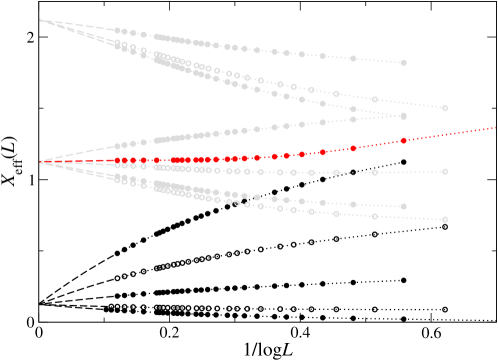
Figure 1: Corrections to the effective scaling dimensions $X_{\mathrm{eff}}=\frac{1}{8}+n$ with $n=0$ (in black) and $1,2$ (in grey) for some of the low-lying states of the $OSp(2|4)$ chain. Data for even (odd) length are presented by filled (open) symbols, data shown in red correspond to a descendent state. Dashed lines are extrapolations to $L\to\infty$.

The subleading logarithmic corrections to scaling, however, vanish with amplitudes depending on $|k|$ as

$$\alpha^{(2|4)}(k)=\frac{1}{4}k^{2}-\frac{7}{16}\,.$$ (24)

Note that these can be related to the corresponding amplitudes observed in spectrum of the periodic $OSp(2|4)$ model, $\beta^{(2|4)}(k)=(k^{2}-1)/8$ Frahm and Martins (2018), by

$$\alpha^{(2|4)}(k)=2\beta^{(2|4)}(k)-\frac{3}{16}\,.$$ (25)

Similar groups of excitations corresponding to primaries with scaling dimension $X=1$ ($2$) appear in the sectors with $n_{1}=2$ and $n_{\pm}=(3\pm k)/2$ for $|k|=0,1,2,\dots\sim(L+1)\mod 2$ ($n_{\pm}=(2\pm k/2)$ for $|k|=0,1,2,\dots\sim L\mod 2$).

In addition we have identified the root configuration for an excitation of the even length superspin chain in the sector $n_{1}=n_{\pm}=1$: apart from the real roots it contains a pair of complex conjugate roots $\lambda_{c\pm}^{(1)}\simeq\lambda_{0}\pm i/2$ with $\lambda_{0}\in\mathbb{R}^{+}$ on the first level and imaginary roots $\lambda_{c}^{(+)}=-\lambda_{c}^{(-)}\simeq i/2$ (or $-i/2$) on the second and third level. Extrapolation of the finite size data gives scaling dimensions $X=1$, see Figure 1, indicating that this is a descendent of the ground state.

III.2 $z=-1$: the $OSp(1|2)$ and $OSP(3|4)$ superspin chains

$OSp(1|2)$.

Solutions of the Bethe equations

$$\left[f_{1/2}\left(\lambda_{j}\right)\right]^{2L}=\prod_{k\neq j}^{L-2n}f_{1}\left(\lambda_{j}-\lambda_{k}\right)f_{1}\left(\lambda_{j}+\lambda_{k}\right)f_{-1/2}\left(\lambda_{j}-\lambda_{k}\right)f_{-1/2}\left(\lambda_{j}+\lambda_{k}\right)\,,\quad j=1,\dots,L-2n\,,$$ (26)

parameterize highest weight states for $(4n+1)$-dimensional $OSp(1|2)$-multiplets with superspin $J=n$ where $2n$ is a non-negative integer. The energy of this state is

$$E=(L-1)-\sum_{j=1}^{L-n}a_{1/2}\left(\lambda_{j}\right)\,.$$ (27)

The lowest levels in each sector with given superspin $J>0$ are given in terms of positive roots of the Bethe equations (26). Among these is the ground state of the $OSp(1|2)$ chain with both even and odd length in the $J=1/2$ triplet sector. From the extrapolation of the finite size energies of this state we reproduce the known central charge $c_{\mathrm{eff}}=-2$ for this model. Up to subleading corrections to scaling this state is degenerate with the $OSp(1|2)$ $J=0$ singlet with a root configuration consisting of $L-2$ positive rapidities and a two-string of complex conjugate ones, $\lambda_{c\pm}\simeq\lambda_{0}\pm i/2$ with $\lambda_{0}\in\mathbb{R}^{+}$. Complemented with results from the finite size analysis of the ground states in the sectors $J>1/2$, we find the conformal weights corresponding to the lowest states with superspin $J$ to be

$$X^{(1|2)}_{J}(L)\simeq J(2J-1)+\frac{\alpha^{(1|2)}(J)}{\log L}\,,\quad J=0,\frac{1}{2},1,\frac{3}{2},\dots\,..$$ (28)

We have identified the lowest excitation in the $J=1/2$ and $1$ sectors: the triplet excitation has a root configuration similar to the $J=0$ ground state described above and corresponds to an operator with conformal weight $X=1$. The excitation on top of the lowest $J=1$ state is given in terms of real roots with a particle-hole pair at the Fermi point giving $X=2$.

The subleading corrections to scaling of some of these states have been studied in Ref. Granet et al. (2019). For the lowest states with superspin $J>0$ they are

$$\alpha^{(1|2)}(J)=-\frac{2}{3}J(J+1)+\frac{5}{24}\,,\quad J=\frac{1}{2},1,\frac{3}{2},\dots\,.$$ (29)

$OSp(3|4)$.

According to (9) these energies do appear in the spectrum of the $OSp(3|4)$ model. The Bethe equations for the latter (in grading $bffbffb$) are

$$\left[f_{1/2}\left({\lambda_{j}^{(1)}}\right)\right]^{2L}=\prod_{k=1}^{N_{2}}f_{1/2}\left({\lambda_{j}^{(1)}-\lambda_{k}^{(2)}}\right)\,f_{1/2}\left({\lambda_{j}^{(1)}+\lambda_{k}^{(2)}}\right)\,,\quad j=1\ldots N_{1}\,,$$ (30)

$$\prod_{k=1}^{N_{1}}f_{1/2}\left(\lambda_{j}^{(2)}-\lambda_{k}^{(1)}\right)\,f_{1/2}\left(\lambda_{j}^{(2)}+\lambda_{k}^{(1)}\right)\,\prod_{k=1}^{N_{3}}f_{1/2}\left({\lambda_{j}^{(2)}-\lambda_{k}^{(3)}}\right)\,f_{1/2}\left({\lambda_{j}^{(2)}+\lambda_{k}^{(3)}}\right)\,$$

$$\qquad=\prod_{k\neq j}^{N_{2}}f_{1}\left({\lambda_{j}^{(2)}-\lambda_{k}^{(2)}}\right)\,f_{1}\left({\lambda_{j}^{(2)}+\lambda_{k}^{(2)}}\right)\,,\quad j=1\ldots N_{2}\,,$$

$$\prod_{k=1}^{N_{2}}f_{1/2}\left(\lambda_{j}^{(3)}-\lambda_{k}^{(2)}\right)\,f_{1/2}\left(\lambda_{j}^{(3)}+\lambda_{k}^{(2)}\right)\,$$

$$\qquad=\prod_{k\neq j}^{N_{3}}f_{1}\left({\lambda_{j}^{(3)}-\lambda_{k}^{(3)}}\right)\,f_{1}\left({\lambda_{j}^{(3)}+\lambda_{k}^{(3)}}\right)\,f_{-1/2}\left({\lambda_{j}^{(3)}-\lambda_{k}^{(3)}}\right)\,f_{-1/2}\left({\lambda_{j}^{(3)}+\lambda_{k}^{(3)}}\right)\,,\quad j=1\dots N_{3}\,.$$

The energy of a state corresponding to a root configuration of (30) is

$$E=-(L-1)+\sum_{j=1}^{L-n}a_{1/2}\left(\lambda_{j}\right)\,.$$ (31)

The root densities for the ground state and low energy excitations of the $OSp(3|4)$ superspin chain are $N_{i}/L\to 1$ in the thermodynamic limit. As in Ref. Frahm and Martins (2018) we label the charge sectors of this model by quantum numbers $(n_{1},n_{2},n_{3})=(N_{1}-N_{2}+1,N_{2}-N_{3}+1,L-N_{1}-2)$. For the low energy states most Bethe roots are arranged in complex conjugate pairs as

$$\lambda^{(1)}_{\pm}\simeq\lambda^{(1)}\pm\frac{5i}{4}\,,\quad\lambda^{(2)}_{\pm}\simeq\lambda^{(2)}\pm\frac{3i}{4}\,,\quad\lambda^{(3)}_{\pm}\simeq\lambda^{(3)}\pm\frac{i}{4}\,,\quad\lambda^{a}\in\mathbb{R}^{+}\,.$$ (32)

The states with lowest energies states are parameterized by configurations with $N_{a}=(L-k-2)/2$ of these strings, i.e. found in the sectors $(n_{1},n_{2},n_{3})=(1,1,k)$ with $k=0,1,2,\dots\sim L\mod 2$. Among them the energies of the $k=0,1$ levels coincide with those of the $J=1/2$ ground state and the lowest $J=0$ state of the $OSp(1|2)$ chain. In the thermodynamic limit all of these states are degenerate giving conformal weights $\lim_{L\to\infty}X^{(3|4)}_{(1,1,k)}(L)=0$, see Figure 2.

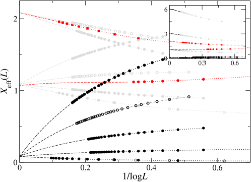
Figure 2: Corrections to the effective scaling dimensions $X_{\mathrm{eff}}=\frac{1}{12}+n$ for the lowest states of the $OSp(3|4)$ superspin chain. The inset shows the lowest levels of the $OSp(1|2)$ model. See Fig. 1 for the meaning of symbols and colors.

From our numerical finite size data we find that this degeneracy is lifted for finite $L$ by subleading corrections to scaling depending on $k$ as

$$X^{(3|4)}_{(1,1,k)}(L)\simeq\frac{\alpha^{(3|4)}(k)}{\log L}\,,\quad\alpha^{(3|4)}(k)=\frac{1}{3}k(k+1)-\frac{7}{24}\,,\quad k=0,1,2,\dots\,.$$ (33)

Note that $\alpha^{(3|4)}(k=0)=\alpha^{(1|2)}(J=\frac{1}{2})$. Comparing these amplitudes to those for the model with periodic boundary conditions Frahm and Martins (2018) we find

$$\alpha^{(3|4)}(k)=2\beta^{(3|4)}(k)-\frac{1}{8}\,.$$ (34)

A group of energies extrapolating to $X^{(3|4)}=1$ is found in the sectors $(n_{1},n_{2},n_{3})=(2,1,k)$ with $k=0,1,2,\dots\sim L+1\mod 2$. Here one of the $N_{1}=L-2-k$ roots on the first level of (30) is real. The energy of the $k=0$ level coincides with the lowest $J=1$ level of the $OSp(1|2)$ chain. The next group of excitations with $X^{(3|4)}=2$ is observed in the sectors $(n_{1},n_{2},n_{3})=(2,2,k)$, $k=0,1,2,\dots\sim L\mod 2$. A summary of the finite size spectrum of the $OSp(1|2)$ and $OSp(3|4)$ is shown in Figure 2.

III.3 $z=0$: the $OSp(2|2)$ superspin chain

The Bethe equations for the $OSp(2|2)$ model (grading $fbbf$) are

$$\left[f_{1/2}\left({\lambda_{j}^{(+)}}\right)\right]^{2L}=\prod_{k=1}^{N_{-}}f_{1}\left({\lambda_{j}^{(+)}-\lambda_{k}^{(-)}}\right)\,f_{1}\left({\lambda_{j}^{(+)}+\lambda_{k}^{(-)}}\right)\,,\quad j=1\ldots N_{+}\,,$$ (35)

$$\left[f_{1/2}\left({\lambda_{j}^{(-)}}\right)\right]^{2L}=\prod_{k=1}^{N_{+}}f_{1}\left({\lambda_{j}^{(-)}-\lambda_{k}^{(+)}}\right)\,f_{1}\left({\lambda_{j}^{(-)}+\lambda_{k}^{(+)}}\right)\,,\quad j=1\ldots N_{-}\,.$$

Each solution to these equations parameterizes an eigenstate of the superspin chain with energy

$$E=(L-1)-\sum_{j=1}^{N_{+}}a_{1/2}\left(\lambda_{j}^{(+)}\right)-\sum_{j=1}^{N_{-}}a_{1/2}\left(\lambda_{j}^{(-)}\right)\,.$$ (36)

The root configurations for the ground state and low energy excitations of the model consist of real roots $\lambda_{j}^{(\pm)}>0$ with densities $N_{\pm}/L\to 1/2$ in the thermodynamic limit. Using quantum numbers $(n_{1},n_{2})=(L-N_{+}-N_{-},N_{+}-N_{-})$ for the $U(1)$ charges we find that the ground state of the model is realized in the $(n_{1},n_{2})=(1,0)$ sector of the superspin chain with odd length. The effective central charge of the model is known to be $c_{\mathrm{eff}}=-1$. In the thermodynamic limit this state degenerates with the lowest levels in the sectors $(n_{1},n_{2})=(1,k)$ for $k=1,2,3,\dots\sim L+1\mod 2$, all of them giving a conformal weight $X_{(1,k)}^{(1|2)}=0$. For finite $L$ the degeneracy is lifted by logarithmic corrections to scaling

$$X^{((2|2)}_{(1,k)}(L)\simeq\frac{\alpha^{(2|2)}(k)}{\log L}\,,\quad\alpha^{(2|2)}(k)=\frac{1}{2}k^{2}-\frac{5}{16}\,.$$ (37)

This expression can be related to that for the periodic $OSp(2|2)$ chain Frahm and Martins (2018) as follows

$$\alpha^{(2|2)}(k)=2\beta^{(2|2)}(k)-\frac{1}{16}\,.$$ (38)

A similar tower of excitations giving conformal weight $X^{(2|2)}=1$ up to logarithmic corrections exists in the sectors $(n_{1},n_{2})=(2,k)$ for $k=0,1,2,\dots\sim L\mod 2$. The finite size scaling behaviour of the states we have analyzed is presented in Figure 3.

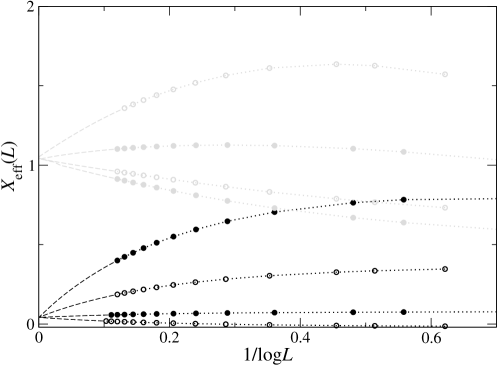
Figure 3: Corrections to the effective scaling dimensions $X_{\mathrm{eff}}=\frac{1}{24}+n$ for the lowest states of the $OSp(2|2)$ chain. See Fig. 1 for the meaning of symbols and colors.

III.4 $z=1$: the $OSp(3|2)$ superspin chain

To study the finite size spectrum of the $OSp(3|2)$ superspin chain we make use of the Bethe equations in two different gradings: the Bethe equations for the model with open boundaries in the grading $fbbbf$ read

$$\left[f_{1/2}\left(\lambda_{j}^{(1)}\right)\right]^{{2L}}=\prod_{k=1}^{{L-n_{1}-n_{2}}}f_{1/2}\left({\lambda_{j}^{(1)}-\lambda_{k}^{(2)}}\right)\,f_{1/2}\left(\lambda_{j}^{(1)}+\lambda_{k}^{(2)}\right)\,,\quad j=1,\cdots,{L-n_{1}},$$ (39)

$$\prod_{k=1}^{{L-n_{1}}}f_{1/2}\left(\lambda_{j}^{(2)}-\lambda_{k}^{(1)}\right)\,f_{1/2}\left(\lambda_{j}^{(2)}+\lambda_{k}^{(1)}\right)=$$

$$\qquad=\prod_{k\neq j}^{{L-n_{1}-n_{2}}}f_{1/2}\left(\lambda_{j}^{(2)}-\lambda_{k}^{(2)}\right)\,f_{1/2}\left(\lambda_{j}^{(2)}+\lambda_{k}^{(2)}\right)\,,\quad j=1,\cdots,{L-n_{1}-n_{2}}\,.$$

The corresponding energy is given in terms of the Bethe roots from the first level as

$$E_{fbbbf}=(L-1)-\sum_{j=1}^{L-n_{1}}a_{1/2}\left(\lambda_{j}^{(1)}\right)\,.$$ (40)

Choosing the grading $bfbfb$ the spectrum of the open superspin chain is parameterized by solutions to the Bethe equations:

$$\left[f_{1/2}\left(\lambda_{j}^{(1)}\right)\right]^{{2L}}=\prod_{k=1}^{{L-n_{1}-n_{2}}}f_{1/2}\left({\lambda_{j}^{(1)}-\lambda_{k}^{(2)}}\right)\,f_{1/2}\left(\lambda_{j}^{(1)}+\lambda_{k}^{(2)}\right)\,,\quad j=1,\cdots,{L-n_{2}-1},$$ (41)

$$\prod_{k=1}^{{L-n_{2}-1}}f_{1/2}\left(\lambda_{j}^{(2)}-\lambda_{k}^{(1)}\right)\,f_{1/2}\left(\lambda_{j}^{(2)}+\lambda_{k}^{(1)}\right)=$$

$$\qquad=\prod_{k\neq j}^{{L-n_{1}-n_{2}}}f_{-1/2}\left(\lambda_{j}^{(2)}-\lambda_{k}^{(2)}\right)\,f_{-1/2}\left(\lambda_{j}^{(2)}+\lambda_{k}^{(2)}\right)\ f_{1}\left(\lambda_{j}^{(2)}-\lambda_{k}^{(2)}\right))\,f_{1}\left((\lambda_{j}^{(2)}+\lambda_{k}^{(2)}\right)\,,$$

$$\qquad\qquad j=1,\cdots,{L-n_{1}-n_{2}}\,,$$

and the corresponding energy eigenvalue is

$$E_{bfbfb}=-L+1+\sum_{j=1}^{L-n_{2}-1}a_{1/2}\left(\lambda_{j}^{(1)}\right)\,.$$ (42)

Solutions to the Bethe equations (39) and (41) parameterize highest weight states of $OSp(3|2)$ in the irreducible representations $(p;q)$ appearing in the tensor product $(0;\frac{1}{2})^{\otimes L}$ of local spins der Jeugt (1984); Frahm and Martins (2015). In terms of the number of Bethe roots the quantum numbers $p$ and $q$ are given as

$$p=n_{1}-1\,,\quad q=(n_{2}+1)/2\,.$$ (43)

Exact diagonalization of the $OSp(3|2)$ Hamiltonian shows that the ground state is a $(p;q)=(0;0)$ singlet ($(0;\frac{1}{2})$ quintet) for $L$ even (odd). Its energy is $E_{0}=Le_{\infty}+f_{\infty}\equiv-3(L-1)$ without any finite size corrections – similar to the model with periodic boundary conditions – giving the effective central charge $c_{\mathrm{eff}}=0$.. The $fbbbf$ Bethe root configuration for $L$ odd contains $(L-1)/2$ pairs of complex conjugate rapidities $\lambda^{(a)}_{j\pm}\simeq\lambda^{(a)}_{j}\pm i/4$ with positive $\lambda^{(a)}_{j}$ on each level $a=1,2$. The root configuration for even $L$ contains degenerate roots.

As for the models considered above the finite size spectrum of the $OSp(3|2)$ superspin chain can be grouped into sets extrapolating to the same integer conformal weight in the thermodynamic limit. Specifically, the lowest states in the sectors $(0;q)$ with $2q=0,1,2,\dots$ (or $(n_{1},n_{2})=(1,k)$ with integer $k$) become degenerate with the ground state, see Figure 4.

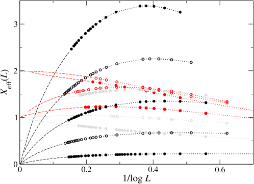
Figure 4: Corrections to the effective scaling dimensions $X_{\mathrm{eff}}=n$ for the lowest excitations of the $OSp(3|2)$ chain in the sectors $(0;q)$ and $(1;q)$ (the ground state in the sectors $(0;0)$, $(0;\frac{1}{2})$ with $X_{\mathrm{eff}}\equiv 0$ independent of $L$ is not shown). See Fig. 1 for the meaning of symbols and colors.

At large but finite $L$ this degeneracy is lifted by logarithmic corrections to scaling

$$X^{(3|2)}_{(0;q)}(L)\simeq\frac{\alpha^{(3|2)}(q)}{\log L}\,,\quad\alpha^{(3|2)}(q)=2q(2q-1)\,.$$ (44)

We note that the amplitudes $\alpha^{(3|2)}$ are twice of those found for the periodic $OSp(3|2)$ chain Frahm and Martins (2015), i.e. $\alpha^{(3|2)}(q)=2\beta^{(3|2)}(q)$.

Finite size data for the lowest states in the sectors $(p;q)=(1;q)$, $q=\frac{1}{2},1,\frac{3}{2}$, and some descendents states are also shown in Figure 4.

IV Discussion

In this paper we have investigated the finite-size properties of the spectrum of the $OSp(n|2m)$ superchain chain with free boundary conditions. We perform this analysis by solving numerically the corresponding Bethe equations for large systems sizes. This study made it possible to identify the corresponding operator content and to extract the amplitudes associated to the subleading corrections to the asymptotic behaviour.

For $z=n-2m<2$ we find that the surface exponents are built out of a set of integer numbers. Similar as in the case of periodic boundary conditions this was to be expected based on the perturbative RG analysis of the model. The surface exponents turn out to be exactly the same as the bulk exponents which is a peculiarity of the underlying universality class. The spectra contain an abundance of states with null conformal dimension whose degeneracy is lifted by subleading logarithmic corrections. We find that the amplitudes of such corrections are different for periodic and free boundary conditions. From our numerical analysis we conjecture a simple relation among these amplitudes to be

$$\alpha(k)=2\beta(k)+\frac{z-1}{16}\,,\qquad z<2\,,$$ (45)

where $\alpha(k)$ and $\beta(k)$ correspond to the amplitudes associated to free and periodic boundaries, respectively.

We now can use this result to infer about the asymptotic behaviour of the surface watermelon correlators associated to the respective loop model. The above relation tells us that we can use the same reference state $k_{0}$ associated to the smallest non-negative amplitudes for both free and periodic boundaries. Proceeding in analogy as has already been explained for periodic boundary Frahm and Martins (2018) we conjecture that the surface correlators should behave as

$$G^{(s)}_{k}(\rho)\sim 1/\ln(\rho)^{2\gamma(k)}\,,\qquad\gamma(k)=\frac{k(k+z-2)}{2-z}\,,$$ (46)

where $\rho$ denotes the distance among two points close to the boundary.

We conclude by recalling some existing results on the finite-size properties in the regime $z\geq 2$ for free boundary conditions. For the $O(2)$ (spin-$1/2$ Heisenberg) model of even length it has been argued that all conformal dimensions are given by the identity conformal tower Alcaraz et al. (1988); Eggert and Affleck (1992). The logarithmic corrections to scaling for this model have been computed in Affleck and Qin (1999). In particular the gap between the ground state and the lowest (triplet) excitation is given by

$$E_{1}^{O(2)}(L)-E_{0}^{O(2)}(L)\simeq\frac{\pi v_{F}}{L}\left(1-1/\ln(L)\right)\,,$$ (47)

corresponding to conformal weight $X=1$ where the amplitude of the logarithmic correction to scaling is determined by the quadratic Casimir of the underlying algebra. The spectrum of the $O(4)$ chain can be composed from the eigenenergies of two decoupled Heisenberg chains Martins and Ramos (1997). This can be used to infer the corresponding behaviour, in particular (note that the Fermi velocities of the $O(2)$ and the $O(4)$ model coincide, see Table 1)

$$E_{1}^{O(4)}(L)-E_{0}^{O(4)}(L)\simeq\frac{\pi v_{F}}{L}\left(1-1/\ln(L)\right)\,.$$ (48)

Based on our previous work on the $OSp(5|2)$ superspin chain with periodic boundary conditions Frahm and Martins (2018) we expect towers of levels with the same conformal weight to be present in the regime $z=n-2m\geq 2$ but $m>0$. We hope to investigate how these degeneracies are lifted by subleading corrections to scaling in a forthcoming paper.

Appendix A The surface energy

To employ Eq. (3) for the analysis of the finite size spectrum of the open $OSp(n|2m)$ superspin chains with free boundary conditions the corresponding surface energy is needed as an input. As a consequence of the spectral inclusion (9) it is sufficient to consider the cases based on the superalgebras $OSp(1|2m)$, $OSp(2|2m)$ and $OSp(3|2)$ for the regime $z=n-2m<2$ considered in the main text. Here the last of these is special due to the singular Bethe root configuration for the ground state, see Section III.4. Based on our numerical results for $OSp(3|2)$ superspin chains of finite length, however, we conclude that the surface energy for this model is $f_{\infty}=3$. The $\mathcal{O}(L^{0})$ contribution to the ground state energy for the other two series of models can be computed using the root density method Yang and Yang (1969); Hamer et al. (1987). We start our discussion below by presenting the main steps of this approach for the $OSp(2|2)$ superspin chain which, as discussed in Section III.3, is solved by a nested Bethe ansatz with real roots for the low energy states. Using similar arguments we then apply this method to derive the surface energies for the spin chains based on $OSp(2|2m)$, $OSp(1|2m)$.

For sake of completeness we also compute the surface energies for the spin chains in the regime $z>2$ (the case $z=2$ can be represented by the isotropic spin-$1/2$ Heisenberg magnet (15) as discussed in the main text). For the models based on the ordinary Lie algebras $O(2n)$ the root density approach can be applied as before. In the case of the $O(2n+1)$ spin chains it has to be modified slightly due to the presence of complex roots in the ground state configuration. For the $O(3)$ and $O(5)$ model we will show at the end of this Appendix, that this can be dealt with using the so-called string hypothesis.

The results obtained in this appendix are summarized in Eqs. (13) and (14).

A.1 $OSp(2|2)$ in the grading $fbbf$

We start by taking the logarithm of the Bethe ansatz equations (35) associated to the $OSp(2|2)$ model for configurations of real roots $\lambda_{j}^{(\pm)}$. As a result we find

$$2L\phi_{1/2}\left(\lambda_{j}^{(+)}\right)=2\pi\mathrm{Q}_{j}^{(+)}+\sum_{k=1}^{N_{-}}\left[\phi_{1}\left(\lambda_{j}^{(+)}-\lambda_{k}^{(-)}\right)+\phi_{1}\left(\lambda_{j}^{(+)}+\lambda_{k}^{(-)}\right)\right],~{}~{}~{}j=1,\dots,N_{+}\,,$$ (49)

$$2L\phi_{1/2}\left(\lambda_{j}^{(-)}\right)=2\pi\mathrm{Q}_{j}^{(-)}+\sum_{k=1}^{N_{+}}\left[\phi_{1}\left(\lambda_{j}^{(-)}-\lambda_{k}^{(+)}\right)+\phi_{1}\left(\lambda_{j}^{(-)}+\lambda_{k}^{(+)}\right)\right],~{}~{}~{}j=1,\dots,N_{-}\,,$$

a1where $\phi_{s}(x)\equiv 2\arctan(x/s)$ and the numbers $\mathrm{Q}_{j}^{(\pm)}$ are positive integers characterizing the possible branches of the logarithm.

From the above Bethe equations the so-called counting functions Yang and Yang (1969)

$$z_{L}^{(+)}(\lambda)=\frac{\phi_{1/2}(\lambda)}{\pi}-\frac{1}{2\pi L}\sum_{k=1}^{N_{-}}\left[\phi_{1}\left(\lambda-\lambda_{k}^{(-)}\right)+\phi_{1}\left(\lambda+\lambda_{k}^{(-)}\right)\right]\,,$$ (50)

$$z_{L}^{(-)}(\lambda)=\frac{\phi_{1/2}(\lambda)}{\pi}-\frac{1}{2\pi L}\sum_{k=1}^{N_{+}}\left[\phi_{1}\left(\lambda-\lambda_{k}^{(+)}\right)+\phi_{1}\left(\lambda+\lambda_{k}^{(+)}\right)\right]\,,$$

take values $z_{L}^{(\pm)}\left(\lambda_{j}^{(\pm)}\right)=\mathrm{Q}_{j}^{(\pm)}/L$ for $j=1,\dots,N_{\pm}$. For the lowest states of the towers considered in Sect. III.3 we have $N_{+}=N_{-}\lesssim L/2$ with uniformly spaced quantum numbers $\mathrm{Q}_{j}^{(\pm)}=j$. Hence densities of the Bethe roots $\lambda_{j}^{(\pm)}$ in these states can be derived from the counting functions as

$$\rho_{L}^{(\pm)}(\lambda)=\frac{d}{d\lambda}z_{L}^{(\pm)}(\lambda)=\frac{a_{1/2}(\lambda)}{\pi}+\frac{1}{2\pi L}a_{1}(\lambda)-\frac{1}{2\pi L}\sum_{k=-N_{\mp}}^{N_{\mp}}a_{1}\left(\lambda-\lambda_{k}^{(\mp)}\right)\,$$ (51)

where we have symmetrized the sums by extending the sets of roots to $\{\lambda_{j}^{(\pm)}\}\cup\{0\}\cup\{\lambda_{-j}^{(\pm)}\equiv-\lambda_{j}^{(\pm)}\}$. Note that these relations are similar to those obtained for periodic boundary conditions except for the presence of the additional boundary terms $a_{1}(\lambda)/(2\pi L)$. We anticipate that these terms are responsible to provide the surface contribution to the ground state energy.

For $L\gg 1$ the extended set of Bethe roots for the ground state tends to a continuous distribution on the entire real axis with densities $\rho_{0}^{(\pm)}(\lambda)$ and the sums in (51) can be replaced by integrals

$$\rho_{0}^{(+)}(\lambda)\simeq\frac{a_{1/2}(\lambda)}{\pi}+\frac{1}{2\pi L}a_{1}(\lambda)-\frac{1}{2\pi}\int_{-\infty}^{+\infty}\mathrm{d}\mu\,a_{1}\left(\lambda-\mu\right)\rho_{0}^{(-)}(\mu)\,,$$ (52)

$$\rho_{0}^{(-)}(\lambda)\simeq\frac{a_{1/2}(\lambda)}{\pi}+\frac{1}{2\pi L}a_{1}(\lambda)-\frac{1}{2\pi}\int_{-\infty}^{+\infty}\mathrm{d}\mu\,a_{1}\left(\lambda-\mu\right)\rho_{0}^{(+)}(\mu)\,.$$

These integral equations can be solved order by order in powers of $L^{-1}$ by elementary Fourier techniques resulting in $\rho^{(\pm)}(\omega)=\sigma_{0}(\omega)+\tau_{0}(\omega)/L$ with

$$\sigma_{0}(\omega)=\frac{1}{\cosh(\omega/2)}\,,\quad\tau_{0}(\omega)=\frac{\exp(-|\omega|)}{1+\exp(-|\omega|)}\,.$$ (53)

Similarly, we rewrite the ground state energy (36) as

$$E_{0}/L\simeq 1-\frac{1}{2}\int_{-\infty}^{\infty}a_{1/2}(\lambda)\left(\rho_{0}^{(+)}(\lambda)+\rho_{0}^{(-)}(\lambda)\right)+\frac{1}{L}\left(-1+a_{1/2}(0)\right)\,.$$ (54)

Using (53) we reproduce the known result $\epsilon_{\infty}=1-4\ln 2$ for the bulk energy density and obtain

$$f_{\infty}=-1+a_{1/2}(0)-2\int_{0}^{\infty}\mathrm{d}\lambda\,a_{1/2}(\lambda)\tau_{0}(\lambda)=3-\int_{-\infty}^{\infty}\mathrm{d}\omega\,\mathrm{e}^{-|\omega|/2}\tau_{0}(\omega)=\pi-1\,$$ (55)

for the surface energy of the $OSp(2|2)$ spin chain as shown in Table 1.

A.2 $OSp(2|2m)$ on the grading $f\dots fbbf\dots f$

For this model the ground state and the low-lying excitations are described in terms real roots in the $f\dots fbbf\dots f$ basis ordering. The Bethe equations are given by

$$\delta_{\ell,1}(2L)\phi_{1/2}\left(\lambda_{j}^{(\ell)}\right)= 2\pi\mathrm{Q}_{j}^{(\ell)}+\sum_{\stackrel{{\scriptstyle k=1}}{{k\neq j}}}^{N_{\ell}}\left[\phi_{1}\left(\lambda_{j}^{(\ell)}-\lambda_{k}^{(\ell)}\right)+\phi_{1}\left(\lambda_{j}^{(\ell)}+\lambda_{k}^{(\ell)}\right)\right]$$ (56)

$$-\sum_{\alpha=\ell\pm 1}\sum_{k=1}^{N_{\alpha}}\left[\phi_{1/2}\left(\lambda_{j}^{(\ell)}-\lambda_{k}^{(\alpha)}\right)+\phi_{1/2}\left(\lambda_{j}^{(\ell)}+\lambda_{k}^{(\alpha)}\right)\right],\quad\ell=1,\dots,m-2\,,$$

$$\delta_{m,2}(2L)\phi_{1/2}\left(\lambda_{j}^{(m-1)}\right)= 2\pi\mathrm{Q}_{j}^{(m-1)}+\sum_{\stackrel{{\scriptstyle k=1}}{{k\neq j}}}^{N_{m-1}}\left[\phi_{1}\left(\lambda_{j}^{(m-1)}-\lambda_{k}^{(m-1)}\right)+\phi_{1}\left(\lambda_{j}^{(m-1)}+\lambda_{k}^{(m-1)}\right)\right]$$

$$-\sum_{{\alpha=m-2,\pm}}\sum_{k=1}^{N_{\alpha}}\left[\phi_{1/2}\left(\lambda_{j}^{(m-1)}-\lambda_{k}^{(\alpha)}\right)+\phi_{1/2}\left(\lambda_{j}^{(m-1)}+\lambda_{k}^{(\alpha)}\right)\right]\,,$$

$$\delta_{m,1}(2L)\phi_{1/2}\left(\lambda_{j}^{(\ell)}\right)= 2\pi\mathrm{Q}_{j}^{(\pm)}+\sum_{k=1}^{N_{\mp}}\left[\phi_{1}\left(\lambda_{j}^{(\ell)}-\lambda_{k}^{(\mp)}\right)+\phi_{1}\left(\lambda_{j}^{(\ell)}+\lambda_{k}^{(\mp)}\right)\right]$$

$$-\sum_{k=1}^{N_{m-1}}\left[\phi_{1/2}\left(\lambda_{j}^{(\ell)}-\lambda_{k}^{(m-1)}\right)+\phi_{1/2}\left(\lambda_{j}^{(\ell)}+\lambda_{k}^{(m-1)}\right)\right],\quad\ell=\pm\,,$$

and the corresponding energy is

$$E=L-1-\sum_{j}a_{1/2}(\lambda^{(1)}_{j})\,.$$ (57)

The ground state is parameterized by $N_{1}=\dots=N_{m-1}=L$ and $N_{\pm}=L/2$ roots distributed on the positive real axis in the thermodynamic limit. Hence, by proceeding as for the $OSp(2|2)$ model above we obtain the $L^{-1}$ boundary contributions $\tau_{0}^{(\ell)}(\lambda)$, $\ell=1,\dots,m-1,\pm$ to the densities. The energy (57) of the $OSp(2|2m)$ superspin chain is given in terms of the first level roots, $\ell=1$. The Fourier representation of their boundary density is

$$\tau_{0}^{(1)}(\omega)=-2\mathrm{e}^{-(m-1)|\omega|/4}\,\frac{\sinh(m|\omega|/4)\cosh(\omega/4)}{\cosh(m\omega/2)}\,.$$ (58)

From (57) the resulting surface energy is given in terms of $\tau_{0}^{(1)}$ as

$$f_{\infty}=-1+\frac{1}{2}a_{1/2}(0)-\int_{0}^{\infty}\mathrm{d}\lambda\,a_{1/2}(\lambda)\tau_{0}^{(1)}(\lambda)=1-\int_{0}^{\infty}\mathrm{d}\omega\,\mathrm{e}^{-|\omega|/2}\tau_{0}^{(1)}(\omega)$$ (59)

After some manipulations with the help of the identity

$$\int_{0}^{+\infty}\frac{\exp(-\mu x)}{\cosh(x)}dx=\frac{1}{2}\Big{(}\psi(\mu/2+1/2)-\psi(\mu/2)\Big{)}\,,$$ (60)

we can rewrite the surface free energy of the $OSp(2|2m)$ superspin chain in terms of the Euler $\psi$ function as presented in the main text (13) with $z=2-2m$.

A.3 $OSp(1|2m)$ on the grading $f\dots fbf\dots f$

In the $f\dots fbf\dots f$ grading the ground state and the low-lying excitations of this model are described in terms of positive rapidities satisfying the Bethe equations

$$\delta_{\ell,1}(2L)\phi_{1/2}\left(\lambda_{j}^{(\ell)}\right)= 2\pi\mathrm{Q}_{j}^{(\ell)}+\sum_{\stackrel{{\scriptstyle k=1}}{{k\neq j}}}^{N_{\ell}}\left[\phi_{1}\left(\lambda_{j}^{(\ell)}-\lambda_{k}^{(\ell)}\right)+\phi_{1}\left(\lambda_{j}^{(\ell)}+\lambda_{k}^{(\ell)}\right)\right]$$ (61)

$$-\sum_{\alpha=\ell\pm 1}\sum_{k=1}^{N_{\alpha}}\left[\phi_{1/2}\left(\lambda_{j}^{(\ell)}-\lambda_{k}^{(\alpha)}\right)+\phi_{1/2}\left(\lambda_{j}^{(\ell)}+\lambda_{k}^{(\alpha)}\right)\right]\,,\quad\ell=1,\dots,m-1\,,$$

$$\delta_{m,1}(2L)\phi_{1/2}\left(\lambda_{j}^{(m)}\right)= 2\pi\mathrm{Q}_{j}^{(m)}+\sum_{\stackrel{{\scriptstyle k=1}}{{k\neq j}}}^{N_{m}}\left[\phi_{1}\left(\lambda_{j}^{(m)}-\lambda_{k}^{(m)}\right)+\phi_{1}\left(\lambda_{j}^{(m)}+\lambda_{k}^{(m)}\right)\right]$$

$$-\sum_{\stackrel{{\scriptstyle k=1}}{{k\neq j}}}^{N_{m}}\left[\phi_{1/2}\left(\lambda_{j}^{(m)}-\lambda_{k}^{(m)}\right)+\phi_{1/2}\left(\lambda_{j}^{(m)}+\lambda_{k}^{(m)}\right)\right]$$

$$-\sum_{k=1}^{N_{m-1}}\left[\phi_{1/2}\left(\lambda_{j}^{(m)}-\lambda_{k}^{(m-1)}\right)+\phi_{1/2}\left(\lambda_{j}^{(m)}+\lambda_{k}^{(m-1)}\right)\right]\,.$$

The energy associated to a solution is given again by (57). In the thermodynamic limit we can introduce densities to describe the root configuration. Solving the corresponding integral equations as above the Fourier expression for the boundary contribution $\tau_{0}^{(1)}$ to the density of first level roots is found to be

$$\tau_{0}^{(1)}(\omega)=-2\mathrm{e}^{-(2m-1)|\omega|/8}\,\frac{\sinh((2m+1)|\omega|/8)\cosh(\omega/4)}{\cosh((2m+1)\omega/4)}\,.$$ (62)

The surface energy of the $OSp(1|2m)$ superspin chain can be computed from (59) which, using (60), can be brought into the form (13) with $z=1-2m$.

A.4 $O(2n)$

As has been discussed in the main text the thermodynamical properties including the surface energy of the $O(2)$ model are known from the studies of the isotropic spin $s=1/2$ Heisenberg model (15). Similarly, the spectrum of the $O(4)$ spin chain can be derived by composing the eigenenergies of two decoupled Heisenberg spin chains Martins and Ramos (1997). From this identification we obtain that the surface free energy of the $O(4)$ spin chain is

$$f_{\infty}^{O(4)}=2f_{\infty}^{O(2)}-1=\pi-2\ln(2)-1\,.$$ (63)

From now on we shall concentrate our analysis for the models with $n\geq 3$. The corresponding Bethe equations are given by

$$\delta_{\ell,1}(2L)\phi_{1/2}\left(\lambda_{j}^{(\ell)}\right)= 2\pi\mathrm{Q}_{j}^{(\ell)}+\sum_{\stackrel{{\scriptstyle k=1}}{{k\neq j}}}^{N_{l}}\left[\phi_{1}\left(\lambda_{j}^{(\ell)}-\lambda_{k}^{(\ell)}\right)+\phi_{1}\left(\lambda_{j}^{(\ell)}+\lambda_{k}^{(\ell)}\right)\right]$$ (64)

$$-\sum_{\alpha=l\pm 1}\sum_{k=1}^{N_{\alpha}}\left[\phi_{1/2}\left(\lambda_{j}^{(\ell)}-\lambda_{k}^{(\alpha)}\right)+\phi_{1/2}\left(\lambda_{j}^{(\ell)}+\lambda_{k}^{(\alpha)}\right)\right]\,,\quad\ell=1,\dots,n-3\,,$$

$$\delta_{n,3}(2L)\phi_{1/2}\left(\lambda_{j}^{(n-2)}\right)= 2\pi\mathrm{Q}_{j}^{(n-2)}+\sum_{\stackrel{{\scriptstyle k=1}}{{k\neq j}}}^{N_{l}}\left[\phi_{1}\left(\lambda_{j}^{(n-2)}-\lambda_{k}^{(n-2)}\right)+\phi_{1}\left(\lambda_{j}^{(n-2)}+\lambda_{k}^{(n-2)}\right)\right]$$

$$-\sum_{\alpha=n-3,\pm}\sum_{k=1}^{N_{\alpha}}\left[\phi_{1/2}\left(\lambda_{j}^{(n-2)}-\lambda_{k}^{(\alpha)}\right)+\phi_{1/2}\left(\lambda_{j}^{(n-2)}+\lambda_{k}^{(\alpha)}\right)\right]\,,$$

$$\delta_{n,2}(2L)\phi_{1/2}\left(\lambda_{j}^{(\ell)}\right)= 2\pi\mathrm{Q}_{j}^{(\pm)}+\sum_{\stackrel{{\scriptstyle k=1}}{{k\neq j}}}^{N_{\pm}}\left[\phi_{1}\left(\lambda_{j}^{(\ell)}-\lambda_{k}^{(\ell)}\right)+\phi_{1}\left(\lambda_{j}^{(\ell)}+\lambda_{k}^{(\ell)}\right)\right]$$

$$-\sum_{k=1}^{N_{n-2}}\left[\phi_{1/2}\left(\lambda_{j}^{(\ell)}-\lambda_{k}^{(n-2)}\right)+\phi_{1/2}\left(\lambda_{j}^{(\ell)}+\lambda_{k}^{(n-2)}\right)\right]\,,\quad\ell=\pm\,.$$

The energy of the corresponding eigenstate of the $O(2n)$ model is given again in terms of the first level roots by the expression (57). The ground state and low lying excitations are parameterized by real roots $\lambda_{j}^{(\ell)}>0$ with total densities $n_{\ell}=N_{\ell}/L=1$ and $n_{\pm}=N_{\pm}/L=1/2$ in the thermodynamic limit. Proceeding as for the models discussed in the previous sections we obtain the Fourier expression for the boundary contribution $\tau_{0}^{(1)}$ to the density of roots $\lambda_{j}^{(1)}$:

$$\tau_{0}^{(1)}(\omega)=-\mathrm{e}^{-(n-2)|\omega|/4}\,\frac{\sinh(n|\omega|/4)-\cosh((n-2)\omega/4)}{\cosh((n-1)\omega/2)}\,.$$ (65)

Using this expression in (59) we find that the surface energy of the $O(2n)$ spin chain is given by (14) with $z=2n$.

A.5 $O(3)$

The Bethe equations for the integrable $O(3)$ spin chain (or, equivalently, the spin $S=1$ Takhtajan-Babujian model Takhtajan (1982); Babujian (1982)) read

$$\left[f_{1/2}(\lambda_{j})\right]^{2L}=\prod_{k\neq j}^{L-n}f_{1/2}(\lambda_{j}-\lambda_{k})f_{1/2}(\lambda_{j}+\lambda_{k})\,,\quad j=1,\dots,L-n\,.$$ (66)

The corresponding energy eigenvalue is given as

$$E=L-1-\sum_{j}^{L-n}a_{1/2}(\lambda_{j})\,.$$ (67)

The ground state of the model for even $L$ is parametrized by a solution of (66) in the sector $n=0$ containing $L/2$ two-strings $x_{j,\pm}\simeq\xi_{j}\pm i/4$, $\xi_{j}>0$. Neglecting corrections to the imaginary parts the Bethe equations can be rewritten in terms of the coordinates of the string centers. Taking the logarithm we obtain

$$2L\left(\phi_{3/4}(\xi_{j})+\phi_{1/4}(\xi_{j})\right)=2\pi\mathrm{Q}_{j}-\phi_{1/2}(\xi_{j})$$ (68)

$$\qquad-\sum_{k=1}^{L/2}\left[2\left(\phi_{1/2}(\xi_{j}-\xi_{k})+\phi_{1/2}(\xi_{j}+\xi_{k})\right)+\phi_{1}(\xi_{j}-\xi_{k})+\phi_{1}(\xi_{j}+\xi_{k})\right]$$

with quantum numbers $\mathrm{Q}_{j}=1,2,\dots,L/2$. Similarly, the energy (67) becomes

$$E_{0}=L-1-\sum_{j=1}^{L/2}\left(a_{1/4}(\xi_{j})+a_{3/4}(\xi_{j})\right)\,.$$ (69)

Proceeding as in Appendix A.1 we obtain an integral equation for the density of strings in the ground state for $L\gg 1$

$$\rho_{0}(\xi)\simeq \frac{1}{\pi}\left(a_{3/4}(\xi)+a_{1/4}(\xi)\right)+\frac{1}{2\pi L}\left(3a_{1/2}(\xi)+a_{1}(\xi)\right)$$ (70)

$$-\frac{1}{2\pi}\int_{-\infty}^{\infty}\mathrm{d}\xi^{\prime}\,\left[2a_{1/2}(\xi-\xi^{\prime})+a_{1}(\xi-\xi^{\prime})\right]\rho_{0}(\xi^{\prime})\,.$$

Solving this integral equation by Fourier methods we obtain

$$\tau_{0}(\omega)=\frac{3+\exp(-|\omega|/2)}{4\cosh^{2}(\omega/4))}$$ (71)

for the $\mathcal{O}(L^{-1})$ contribution to the density. Hence we have

$$f_{\infty} =-1+\frac{1}{2}\left(a_{1/4}(0)+a_{3/4}(0)\right)-\int_{0}^{\infty}\mathrm{d}\xi\,\left(a_{1/4}(\xi)+a_{3/4}(\xi)\right)\tau_{0}(\xi)$$ (72)

$$=\frac{13}{3}-\int_{0}^{\infty}\mathrm{d}\omega\,\left(\mathrm{e}^{-|\omega|/4}+\mathrm{e}^{-3|\omega|/4}\right)\tau_{0}(\omega)=2\pi-5\,.$$

which coincides with (14) for $z=3$ (the same result has recently been obtained using a slightly different method in Zheng et al. (2022)).

A.6 $O(5)$

The Bethe equations for the $O(5)$ model read

$$\left[f_{1/2}(\lambda^{(1)}_{j})\right]^{2L}=\prod_{k\neq j}^{L-n_{1}}f_{1}(\lambda^{(1)}_{j}-\lambda^{(1)}_{k})f_{1}(\lambda^{(1)}_{j}+\lambda^{(1)}_{k})\prod_{k=1}^{L-n_{1}-n_{2}}f_{-1}(\lambda^{(1)}_{j}-\lambda^{(2)}_{k})f_{-1}(\lambda^{(1)}_{j}+\lambda^{(2)}_{k})\,,$$ (73)

$$\qquad\qquad j=1,\dots,L-n_{1}\,,$$

$$\prod_{k\neq j}^{L-n_{1}-n_{2}}f_{1/2}(\lambda^{(2)}_{j}-\lambda^{(2)}_{k})f_{1/2}(\lambda^{(2)}_{j}+\lambda^{(2)}_{k})=\prod_{k=1}^{L-n_{1}}f_{1/2}(\lambda^{(2)}_{j}-\lambda^{(1)}_{k})f_{1/2}(\lambda^{(2)}_{j}+\lambda^{(1)}_{k})\,,$$

$$\qquad\qquad j=1,\dots,L-n_{1}-n_{2}\,.$$

The ground state for even length spin chains is in the sector $(n_{1},n_{2})=(0,0)$ with $\lambda^{(1)}_{j}\in\mathbb{R}^{+}$ and $\lambda^{(2)}_{j}$ arranged in 2-strings $\lambda^{(2)}_{j}\simeq\xi_{j}\pm i/4$, $\xi_{j}>0$. The corresponding energy is again given by (57). Following the same steps as for the $O(3)$ model above we obtain Bethe equations for the string coordinates from (73)

$$2L\phi_{1/2}(\lambda^{(1)}_{j})=2\pi\mathrm{Q}_{j}-\phi_{1/2}(\lambda^{(1)}_{j})+\sum_{k=1}^{L}\left(\phi_{1}(\lambda^{(1)}_{j}-\lambda^{(1)}_{k})+\phi_{1}(\lambda^{(1)}_{j}+\lambda^{(1)}_{k})\right)$$ (74)

$$\qquad-\sum_{k=1}^{L/2}\left[\phi_{3/4}(\lambda^{(1)}_{j}-\xi_{k})+\phi_{3/4}(\lambda^{(1)}_{j}+\xi_{k})+\phi_{1/4}(\lambda^{(1)}_{j}-\xi_{k})+\phi_{1/4}(\lambda^{(1)}_{j}+\xi_{k})\right]\,,\quad j=1,\dots,L\,,$$

$$\sum_{k=1}^{L}\left[\phi_{3/4}(\xi_{j}-\lambda^{(1)}_{k})+\phi_{3/4}(\xi_{j}+\lambda^{(1)}_{k})+\phi_{1/4}(\xi_{j}-\lambda^{(1)}_{k})+\phi_{1/4}(\xi_{j}+\lambda^{(1)}_{k})\right]$$

$$\qquad=2\pi\overline{\mathrm{Q}}_{j}-\phi_{1/2}(\xi_{j})+\sum_{k=1}^{L/2}\left[\phi_{1}(\xi_{j}-\xi_{k})+\phi_{1}(\xi_{j}+\xi_{k})+2\left(\phi_{1/2}(\xi_{j}-\xi_{k})+\phi_{1/2}(\xi_{j}+\xi_{k})\right)\right]\,,$$

$$\qquad\qquad j=1,\dots,L/2\,.$$

For $L\gg 1$ the ground state densities $\rho_{0}(\lambda)$ of real roots from the first level Bethe equations and $\overline{\rho}_{0}(\xi)$ of two-strings from the second one are given in terms of the integral equations

$$\rho_{0}(\lambda)= \frac{1}{\pi}a_{1/2}(\lambda)+\frac{1}{2\pi L}\left(a_{1}(\lambda)-a_{3/4}(\lambda)+a_{1/2}(\lambda)-a_{1/4}(\lambda)\right)$$ (75)

$$-\frac{1}{2\pi}\int_{-\infty}^{\infty}\mathrm{d}\lambda^{\prime}\,a_{1}(\lambda-\lambda^{\prime})\rho(\lambda^{\prime})+\frac{1}{2\pi}\int_{-\infty}^{\infty}\mathrm{d}\xi^{\prime}\,\left[a_{3/4}(\lambda-\xi^{\prime})+a_{1/4}(\lambda-\xi^{\prime})\right]\overline{\rho}_{0}(\xi)\,,$$

$$\overline{\rho}_{0}(\xi)= \frac{1}{2\pi L}\left(a_{1}(\xi)-a_{3/4}(\xi)+3a_{1/2}(\xi)-a_{1/4}(\xi)\right)+\frac{1}{2\pi}\int_{-\infty}^{\infty}\mathrm{d}\lambda^{\prime}\,\left[a_{3/4}(\xi-\lambda^{\prime})+a_{1/4}(\xi-\lambda^{\prime})\right]\rho_{0}(\lambda^{\prime})$$

$$-\frac{1}{2\pi}\int_{-\infty}^{\infty}\mathrm{d}\xi^{\prime}\,\left[2a_{1/2}(\xi-\xi^{\prime})+a_{1}(\xi-\xi^{\prime})\right]\overline{\rho}_{0}(\xi^{\prime})\,.$$

Solving these equations the boundary contribution to the density $\rho_{0}$ of first level roots is found to be

$$\tau_{0}(\omega)=-\mathrm{e}^{-|\omega|/8}\,\frac{\sinh(5|\omega|/8)-\cosh(\omega/8)}{\cosh(3\omega/4)}\,.$$ (76)

Using this expression in (59) yields the resulting surface energy of the $O(5)$ spin chain (and the $OSp(n|2m)$ superspin chains with $n-2m=5$)

$$f_{\infty}=-1+\frac{2\sqrt{3}}{9}\pi+\frac{\pi}{3}+\frac{1}{3}\left(\psi\left(\frac{5}{12}\right)-\psi\left(\frac{11}{12}\right)\right)\,$$ (77)

in agreement with Eq. (14) for $z=5$.

References

• Gade (1999) R. M. Gade, “An integrable $sl(2|1)$ vertex model for the spin quantum Hall critical point,” J. Phys. A: Math. Gen. 32, 7071–7082 (1999).
• Essler et al. (2005) F. H. L. Essler, H. Frahm,  and H. Saleur, “Continuum limit of the integrable $sl(2/1)$ $3$-$\bar{3}$ superspin chain,” Nucl. Phys. B 712 [FS], 513–572 (2005), cond-mat/0501197 .
• Martins et al. (1998) M. J. Martins, B. Nienhuis,  and R. Rietman, “An Intersecting Loop Model as a Solvable Super Spin Chain,” Phys. Rev. Lett. 81, 504–507 (1998), cond-mat/9709051 .
• Jacobsen et al. (2003) J. L. Jacobsen, N. Read,  and H. Saleur, “Dense Loops, Supersymmetry, and Goldstone Phases in Two Dimensions,” Phys. Rev. Lett. 90, 090601 (2003), cond-mat/0205033 .
• Frahm and Martins (2018) H. Frahm and M. J. Martins, “The fine structure of the finite-size effects for the spectrum of the $OSp(n|2m)$ spin chain,” Nucl. Phys. B 930, 545–562 (2018), arXiv:1802.05191 .
• Saleur and Schomerus (2007) H. Saleur and V. Schomerus, “On the $SU(2|1)$ WZW model and its statistical mechanics applications,” Nucl. Phys. B 775, 312–340 (2007), hep-th/0611147 .
• Ikhlef et al. (2008) Y. Ikhlef, J. L. Jacobsen,  and H. Saleur, “A staggered six-vertex model with non-compact continuum limit,” Nucl. Phys. B 789, 483–524 (2008), cond-mat/0612037 .
• Frahm and Martins (2011) H. Frahm and M. J. Martins, “Finite size properties of staggered ${U}_{q}[sl(2|1)]$ superspin chains,” Nucl. Phys. B 847, 220–246 (2011), arXiv:1012.1753 .
• Frahm and Martins (2012) H. Frahm and M. J. Martins, “Phase Diagram of an Integrable Alternating ${U}_{q}[sl(2|1)]$ Superspin Chain,” Nucl. Phys. B 862, 504–552 (2012), arXiv:1202.4676 .
• Frahm and Hobuß (2017) H. Frahm and K. Hobuß, “Spectral flow for an integrable staggered superspin chain,” J. Phys. A: Math. Theor. 50, 294002 (2017), arXiv:1703.08054 .
• Vernier et al. (2014a) É. Vernier, J. L. Jacobsen,  and H. Saleur, “Non compact conformal field theory and the $a_{2}^{(2)}$ (Izergin-Korepin) model in regime III,” J. Phys. A: Math. Theor 47, 285202 (2014a), arXiv:1404.4497 .
• Vernier et al. (2014b) É. Vernier, J. L. Jacobsen,  and H. Saleur, “Non compact continuum limit of two coupled Potts models,” J. Stat. Mech. , P10003 (2014b), arXiv:1406.1353 .
• Vernier et al. (2016) E. Vernier, J. L. Jacobsen,  and H. Saleur, “The continuum limit of $a_{N-1}^{(2)}$ spin chains,” Nucl. Phys. B 911, 52–93 (2016), arXiv:1601.01559 .
• Frahm et al. (2019) H. Frahm, K. Hobuß,  and M. J. Martins, “On the critical behaviour of the integrable q𝑞q-deformed O​S​p​(3|2)𝑂𝑆𝑝conditional32{OSp(3|2)} superspin chain,” Nucl. Phys. B 946, 114697 (2019), arXiv:1906.00655 .
• Frahm and Martins (2015) H. Frahm and M. J. Martins, “Finite-size effects in the spectrum of the ${OS}p(3|2)$ superspin chain,” Nucl. Phys. B 894, 665–684 (2015), arXiv:1502.05305 .
• Polyakov (1975) A. M. Polyakov, “Interaction of goldstone particles in two dimensions. Applications to ferromagnets and massive Yang-Mills fields,” Phys. Lett. B 59, 79–81 (1975).
• Nahum et al. (2013) A. Nahum, P. Serna, A. M. Somoza,  and M. OrtuĂąo, “Loop models with crossings,” Phys. Rev. B 87, 184204 (2013), arXiv:1303.2342 .
• Cardy (1984) J. L. Cardy, “Conformal invariance and surface critical behavior,” Nucl. Phys. B 240 [FS12], 514–532 (1984).
• Cardy (1986a) J. L. Cardy, “Effect of boundary conditions on the operator content of two-dimensional conformally invariant theories,” Nucl. Phys. B 275, 200–218 (1986a).
• Robertson et al. (2020) N. F. Robertson, M. Pawelkiewicz, J. L. Jacobsen,  and H. Saleur, “Integrable boundary conditions in the antiferromagnetic potts model,” JHEP 2020, 144 (2020), arXiv:2003.03261 .
• Robertson et al. (2021) N. F. Robertson, J. L. Jacobsen,  and H. Saleur, “Lattice regularisation of a non-compact boundary conformal field theory,” JHEP 2102, 180 (2021), arXiv:2012.07757 .
• Frahm and Gehrmann (2022) H. Frahm and S. Gehrmann, “Finite size spectrum of the staggered six-vertex model with uq​(𝔰​𝔩​(2))subscript𝑢𝑞𝔰𝔩2u_{q}(\mathfrak{sl}(2))-invariant boundary conditions,” JHEP , 01, 070 (2022), arXiv:2111.00850 .
• BlĂśte et al. (1986) H. W. J. BlĂśte, J. L. Cardy,  and M. P. Nightingale, “Conformal invariance, the central charge and universal finite-size amplitudes at criticality,” Phys. Rev. Lett. 56, 742–745 (1986).
• Cardy (1986b) J. L. Cardy, “Logarithmic corrections to finite-size scaling in strips,” J. Phys. A: Math. Gen. 19, L1093–L1098 (1986b).
• Affleck and Qin (1999) I. Affleck and S. Qin, “Logarithmic Corrections in Quantum Impurity Problems,” J. Phys. A: Math. Gen. 32, 7815–7826 (1999), cond-mat/9907284 .
• Duplantier and Saleur (1986) B. Duplantier and H. Saleur, “Exact surface and wedge exponents for polymers in two dimensions,” Phys. Rev. Lett. 57, 3179–3182 (1986).
• Martins and Ramos (1997) M. J. Martins and P. B. Ramos, “The algebraic Bethe ansatz for rational braid-monoid lattice models,” Nucl. Phys. B 500, 579–620 (1997), hep-th/9703023 .
• Sklyanin (1988) E. K. Sklyanin, “Boundary conditions for integrable quantum systems,” J. Phys. A: Math. Gen. 21, 2375–2389 (1988).
• Arnaudon et al. (2003) D. Arnaudon, J. Avan, N. Crampe’, A. Doikou, L. Frappat,  and E. Ragoucy, “Classification of reflection matrices related to (super) Yangians and application to open spin chain models,” Nucl. Phys. B 668, 469–505 (2003), math/0304150 .
• Arnaudon et al. (2004) D. Arnaudon, J. Avan, N. Crampe, A. Doikou, L. Frappat,  and E. Ragoucy, “Bethe Ansatz equations and exact S𝑆{S} matrices for the o​s​p​(M|2​n)𝑜𝑠𝑝conditional𝑀2𝑛{osp(M|2n)} open super spin chain,” Nucl. Phys. B 687, 257–278 (2004), math-ph/0310042 .
• Yang and Yang (1969) C. N. Yang and C. P. Yang, “Thermodynamics of a one-dimensional system of bosons with repulsive delta-function interaction,” J. Math. Phys. 10, 1115–1122 (1969).
• HulthĂŠn (1939) L. HulthĂŠn, “Über das Austauschproblem eines Kristalles,” Arkiv Mat. Astron. Fys. 26A, 1–105 (1939).
• Hamer et al. (1987) C. J. Hamer, G. R. W. Quispel,  and M. T. Batchelor, “Conformal anomaly and surface energy for Potts and Ashkin-Teller quantum chains,” J. Phys. A: Math. Gen. 20, 5677–5693 (1987).
• Affleck (1986) I. Affleck, “Universal term in the free energy at a critical point and and the conformal anomaly,” Phys. Rev. Lett. 56, 746–748 (1986).
• Cardy (1986c) J. L. Cardy, “Operator content of two-dimensional conformally invariant theories,” Nucl. Phys. B 270, 186–204 (1986c).
• Granet et al. (2019) E. Granet, J. L. Jacobsen,  and H. Saleur, “Spontaneous symmetry breaking in 2D supersphere sigma models and applications to intersecting loop soups,” J. Phys. A: Math. Theor 52, 345001 (2019), arXiv:1810.07807 .
• der Jeugt (1984) J. V. der Jeugt, “Finite- and infinite-dimensional representations of the orthosymplectic superalgebra OSP(3,2),” J. Math. Phys. 25, 3334–3349 (1984).
• Alcaraz et al. (1988) F. C. Alcaraz, M. Baake, U. Grimmn,  and V. Rittenberg, “Operator content of the XXZ chain,” J. Phys. A: Math. Gen. 21, L117–L120 (1988).
• Eggert and Affleck (1992) S. Eggert and I. Affleck, “Magnetic impurities in half-integer-spin Heisenberg antiferromagnetic chains,” Phys. Rev. B 46, 10866–10883 (1992).
• Takhtajan (1982) L. Takhtajan, “The picture of low–lying excitations in the isotropic Heisenberg chain of arbitrary spins,” Phys. Lett. A 87, 479–482 (1982).
• Babujian (1982) H. M. Babujian, “Exact solution of the one–dimensional isotropic Heisenberg chain with arbitrary spin ${S}$,” Phys. Lett. A 90, 479–482 (1982).
• Zheng et al. (2022) Z. Zheng, P. Sun, X. Xu, T. Yang, J. Cao,  and W.-L. Yang, “Thermodynamic limit and boundary energy of the spin-1 Heisenberg chain with non-diagonal boundary fields,” SciPost Phys. 12, 71 (2022).