Magneto-optical rotation: Accurate approximated analytical solutions for single-probe atomic magnetometers

Abstract

We report an approximated analytical solution for a single-probe four-state atomic magnetometer where no analytical solution exists. This approximated analytical solution demonstrates excellent accuracy in broad probe power and detuning ranges when compared with the numerical solution obtained using a 4th order Runge-Kutta differential equation solver on MATLAB. The theoretical framework and results also encompass widely applied single-probe three-state atomic magnetometers for which no analytical solution, even approximated, is available to date in small detuning regions.

Magneto-optical Faraday rotation describes the rotation of the polarization plane of a linearly polarized light field traversing through a magnetized medium r1 . When a laser was first used as the light source, it was found that the angle of polarization plane rotation was dependent upon the intensity of the laser, hence given the term “nonlinear magneto-optical rotation effect” (NMORE) r2 . For the past 60 years, atomic NMORE studies have primarily focused on a single probe laser interacting with $F=1$ atomic systems r3 ; r4 ; r5 , Many pioneering studies and innovations r6 ; r7 ; r8 ; r9 ; r10 ; r11 ; r12 ; r13 ; r14 have contributed to the advancement in this research field. However, to date there has been no analytic solution$-$or even an approximated analytic solution with sufficient accuracy$-$for NMORE phenomena. This is especially the case when the laser is tuned close to the relevant one-photon resonance in order to enhance the observability of NMORE signal r7 . Such a near resonance excitation inevitably introduces significant power broadening, rendering analytic solutions very difficult. Consequently, only numerical solutions are available for such near resonance excitation operations r3 . Recent experimental and theoretical progress r15a ; r15 , especially the demonstration of an NMORE blockade in a single-probe configuration, has for the first time opened the possibility for analytical or approximated analytical solutions with high accuracy for single-probe NMOREs.

In this work we show a high-accuracy approximate analytical solution for widely studied single-probe atomic systems. The theoretical framework presented here encompasses both three and four-state systems for both near and far-detuned optical fields [see Fig. 1(a)].

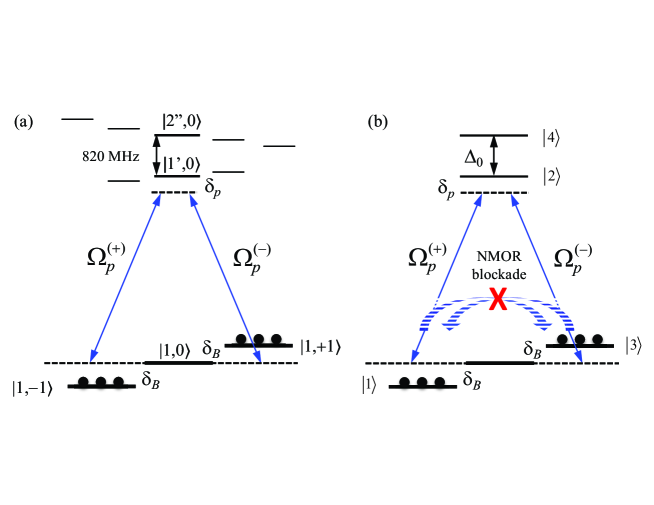
Figure 1: (a) Rubidium D-1 transitions relevant to single-probe atomic magnetometers. (b) A four-state model single-probe atomic magnetometer. Dashed blue arrows represent two opposite two-photon transitions. Population symmetry as well as transition symmetry lead to a NMORE blockade that strongly suppresses NMORE signal.

We consider a four-state atomic system, depicted in Fig. 1(b), where the atomic state $|j\rangle$ has energy $\hbar\omega_{j}$ ($j=1,...,4$) and the lower three states form an $F=1$ system. We assume that the probe field $\mathbf{E}_{p}$ (frequency $\omega_{p}$) is polarized along the $\hat{x}$-axis and propagates along the $\hat{z}$-axis. Its $\sigma^{(\pm)}$ components independently couple the $|1\rangle\Leftrightarrow|2\rangle$ and $|3\rangle\Leftrightarrow|2\rangle$ transitions with a large one-photon detuning $\delta_{2}=\omega_{p}-[\omega_{2}-(\omega_{1}+\omega_{3})/2]=\delta_{p}$. The second excited state $|4\rangle$ is assumed to be $\Delta_{0}$ above the state $|2\rangle$, enabling the second excitation channel by the same probe field with a detuning of $\delta_{4}=\omega_{p}-[\omega_{4}-(\omega_{1}+\omega_{3})/2]=\delta_{p}+\Delta_{0}$ (in our notation $\delta_{p}<0$ and $\Delta_{0}=-\omega_{4}+\omega_{2}<0$). This atomic system describes, for example the Rubidium D-1 line with a hyper-fine splitting, i.e., $|2\rangle=|5P_{1/2},F^{\prime}=1\rangle$ and $|4\rangle=|5P_{1/2},F^{\prime}=2\rangle$ with $|\Delta_{0}|=820$ MHz [Fig. 1(a)]. Since initially the population is equally shared by the two ground states $|F=1,m_{F}=\pm 1\rangle$, therefore two opposite two-photon transitions between states $|1\rangle$ and $|3\rangle$ with a two-photon detuning $2\delta_{B}$ are simultaneously established. Here, the circular components of the probe field simultaneously access excited states $|2\rangle$ and $|4\rangle$ with different excitation rates. The magnetic field induced Zeeman frequency shift $\delta_{B}=g\mu_{0}B$ in the axial magnetic field $B=B_{z}$ is defined with respect to the mid-point between the two equally but oppositely shifted Zeeman levels $|1\rangle=|m_{F}=-1\rangle$ and $|3\rangle=|m_{F}=+1\rangle$.

Under the electric-dipole approximation, the system interaction Hamiltonian reads

$$\frac{\hat{H}}{\hbar}\!=\!\sum_{j=1}^{4}\delta_{j}|j\rangle\langle j|\!+\!\sum_{m=2,4}\!\left[\Omega_{m1}|m\rangle\langle 1|\!+\!\Omega_{m3}|m\rangle\langle 3|\!+\!{\rm c.c}\right],\>$$ (1)

where $\delta_{j}$ is the laser detuning from state $|j\rangle$. The total electric field is given by $\mathbf{E}\!=\!\left(\mathbf{\hat{e}}_{+}{\cal E}_{p}^{(+)}\!+\!\mathbf{\hat{e}}_{-}{\cal E}_{p}^{(-)}\right){\rm e}^{i\theta_{p}}\!+\!{\rm c.c.}$ where $\theta_{p}\!=\!\mathbf{k}_{p}\!\cdot\mathbf{r}-\omega_{p}t$ with $k_{p}\!=\omega_{p}/c$ being the wavevector of the field. Expressing probe Rabi frequencies with respect to the state $|2\rangle$ as $\Omega_{21}\!=\!\Omega_{p}^{(+)}\!=\!D_{21}{\cal E}_{p}^{(+)}/2\hbar$ and $\Omega_{23}\!=\!\Omega_{p}^{(-)}\!=\!D_{23}{\cal E}_{p}^{(-)}/2\hbar$, we then have $\Omega_{41}\!=\!D_{41}{\cal E}_{p}^{(+)}/(2\hbar)\!=\!d_{42}\Omega_{p}^{(+)}$ and $\Omega_{43}\!=\!D_{43}{\cal E}_{p}^{(-)}/(2\hbar)\!=\!d_{42}\Omega_{p}^{(-)}$. Here, we define $d_{42}=D_{41}/D_{21}=D_{43}/D_{23}$ with $D_{nm}=\langle n|\hat{D}|m\rangle$ being the transition matrix element of the dipole operator $\hat{D}$ and $D_{21}=D_{23}$, $D_{41}=D_{43}$.

Under rotating wave approximation, the Schrodinger equations describing wave-function amplitudes are,

$$\dot{A}_{1}-i\delta_{B}A_{1}=i{\Omega_{p}^{(+)}}^{*}\left(A_{2}+d_{42}A_{4}\right)-\gamma A_{1},$$ (2a)

$$\dot{A}_{3}+i\delta_{B}A_{3}=i{\Omega_{p}^{(-)}}^{*}\left(A_{2}+d_{42}A_{4}\right)-\gamma A_{3},$$ (2b)

$$\dot{A}_{2}-i\delta_{p}A_{2}=i\Omega_{p}^{(+)}A_{1}+i\Omega_{p}^{(-)}A_{3}-\Gamma A_{2},$$ (2c)

$$\dot{A}_{4}\!-\!i\!\left(\delta_{p}\!-\!\Delta_{0}\right)\!A_{4}\!=\!id_{42}\!\left(\Omega_{p}^{(+)}A_{1}\!+\!\Omega_{p}^{(-)}A_{3}\right)\!-\!\Gamma\!A_{4},$$ (2d)

where for simplicity we have expressed the ground and excited states’ decay rates as $\gamma$ and $\Gamma$, respectively.

Applying the slowly varying envelope approximation and the third-order perturbation calculation r15 ; r16 , we obtain the Maxwell equations describing the evolution of both circular polarized components of the probe field $\mathbf{E}_{p}$ in the moving frame ($\xi=z-ct$, $\eta=z$),

$$\frac{\partial\Omega_{p}^{(\pm)}}{\partial\eta}\approx-\sum_{n=2,4}\alpha_{n}\Omega_{p}^{(\pm)}\!+\!\sum_{n=2,4}\!\frac{\alpha_{n}}{2}(1+id_{n})S_{\mp}\Omega_{p}^{(\pm)}\!\!\left(\!\frac{\Gamma_{0}\!+\!i\beta_{0}}{\Gamma_{-}\!+\!i\beta_{-}}\!+\!\frac{\Gamma_{0}\!-\!i\beta_{0}}{\Gamma_{+}\!+\!i\beta_{+}}\!\right),$$ (3)

where $\alpha_{n}=\kappa_{n}/\Gamma(1+d_{n}^{2})$, $\kappa_{2}=\kappa_{23}$ and $\kappa_{4}=\kappa_{43}$ ($\kappa_{2}=2\pi|D_{21}|^{2}{\cal N}_{0}\omega_{p}/(\hbar c)$ where ${\cal N}_{0}$ is the atom number density). The first summation on the right accounts for the linear absorption (we have neglected the linear propagation phase shift since it does not contribute to NMORE). The normalized detunings are defined as $d_{2}=\delta_{p}/\Gamma$, $d_{4}=(\delta_{p}-\Delta_{0})/\Gamma$, and $d_{B}=\delta_{B}/\gamma$. In addition, we have defined $\beta_{\pm}=-d_{B}\mp\beta_{0}S^{(\pm)}$, $\Gamma_{\pm}=1+\Gamma_{0}S^{(\pm)}$, $\beta_{0}=d_{2}/(1+d_{2}^{2})+d_{4}/(1+d_{4}^{2})$, and $\Gamma_{0}=1/(1+d_{2}^{2})+1/(1+d_{4}^{2})$ where $\beta_{0}$ and $\Gamma_{0}$ are the total light induced frequency shift and resonance broadening, respectively. The probe two-photon saturation parameters are defined as $S_{\pm}=|\Omega_{p}^{(\pm)}|^{2}/\gamma\Gamma$. Letting $\Omega_{p}^{(\pm)}=R_{\pm}\,e^{i\theta_{\pm}}$ where $R_{\pm}$ and $\theta_{\pm}$ are real quantities, then Eq. (3) gives

$$\frac{\partial S_{\pm}}{\partial\eta}=-\alpha S_{\pm}\!+\!S_{+}S_{-}{\cal P}_{\pm},$$ (4a)

$$\frac{\partial\theta_{\pm}}{\partial\eta}=\frac{S_{\mp}}{2}{\cal Q}_{\pm}.$$ (4b)

where ${\cal P}_{\pm}=\alpha{\cal A}\mp\alpha_{d}{\cal B}$, ${\cal Q}_{\pm}=\mp\alpha{\cal B}+\alpha_{d}{\cal A}$ with ${\cal A}\!=\!\Gamma_{0}(\Gamma_{-}/G_{-}\!+\!\Gamma_{+}/G_{+}\!)$, ${\cal B}\!=\!\Gamma_{0}(\beta_{-}/G_{-}\!+\!\beta_{+}/G_{+}\!)$, $\alpha=\alpha_{2}+\alpha_{4}$, $\alpha_{d}=d_{2}\alpha_{2}+d_{4}\alpha_{4}$, and $G_{\pm}=\Gamma_{\pm}^{2}+\beta_{\pm}^{2}$ (in the following calculations and without the loss of generality we neglect $\beta_{0}$ terms r17 ). The advantage of this photon number representation is that intensity [i.e., Eq. (4a)] decouples from the phase [i.e., Eq. (4b)]. While both Eqs. (4a) and (4b) are highly nonlinear and complex, approximated analytical solutions can be obtained with excellent accuracy. As we show below, two key steps separately based on the physics of the single-probe system and mathematical considerations for approximation accuracy are necessary to achieve this.

The first key step is to realize the presence of a symmetry-enforced NMORE blockade in any single-probe system where population and transition symmetry are present r18a . We note that the probe field is the only energy source and therefore its two circular components must add up at any propagation distance to give $S_{-}(\eta)=S_{0}e^{-\alpha\eta}-S_{+}(\eta)$ where $S_{0}=\Omega_{p}(0)^{2}/\gamma\Gamma$ is the initial total energy of the single probe field. Taking the differential equation for the $S_{+}$ component in Eq. (4a) and inserting this energy restriction relation into intensity product in the second term on the right side of Eq. (4a), we immediately conclude a gain-clamping effect, i.e., $(S_{0}e^{-\alpha\eta}-S_{+})S_{+}$. This energy constraint locks the two probe components by enacting a self-restricted growth, resulting in $S_{\pm}(\eta)\approx S_{\pm}(0)$. That is, no appreciable magnetic field induced optical field change is allowed for either component (see numerical results and discussion later) r18 . It is this propagation growth restriction that limits the single-probe NMORE to be in characteristically linear. This is a single-probe NMORE blockade first postulated in Ref.r15a and then demonstrated mathematically in Ref.r15 . As we show below, it is this NMORE blockade and the linear absorption characteristics of both field components that lead to a high-accuracy approximate analytical solution that is well-applicable to both three and four-state atomic systems.

The second key step is based on the mathematics consideration of ${\cal P}_{\pm}$ and ${\cal Q}_{\pm}$ which contain $S_{\pm}(\eta)$. One of the consequences of the above described NMORE blockade is that the dominant propagation behavior is determined by linear absorption since the gain is clamped. The magnetic field is contained in functions ${\cal P}_{\pm}$ and ${\cal Q}_{\pm}$, and its effect should mostly be near magnetic resonance. Therefore, it is a reasonable expectation that errors by replacing $S_{\pm}(\eta)$ in ${\cal P}_{\pm}$ and ${\cal Q}_{\pm}$ with $S_{\pm}(\eta)\rightarrow(S_{0}/2)e^{-\alpha\eta}$ should be relatively small. Therefore, as the first trial we set $S_{\pm}(\eta)=(S_{0}/2)e^{-\alpha\eta}$ in denominators of ${\cal P}_{\pm}$ and ${\cal Q}_{\pm}$.

The major benefit of the second step is that now both ${\cal P}_{\pm}$ and ${\cal Q}_{\pm}$ contain $e^{-\alpha\eta}$ only, permitting analytical solutions to both field and NMORE. We get

$$S_{\pm}(\eta;d_{B})=\frac{S_{0}e^{S_{0}\Gamma_{0}{\cal L}_{\pm}}}{1+S_{0}e^{S_{0}\Gamma_{0}{\cal L}_{\pm}}}e^{-\alpha\eta},$$ (5)

where

$${\cal L}_{\pm}(\eta;d_{B})=2\Gamma_{0}\int_{0}^{\eta}\frac{\alpha(1+\Gamma_{0}S_{0}e^{-\alpha\eta}/2)\mp\alpha_{d}d_{B}}{d_{B}^{2}+(1+\Gamma_{0}S_{0}e^{-\alpha\eta}/2)^{2}}d\eta,$$

is analytically integrable. Inserting Eq. (5) into Eq. (4b), we obtain

$$\theta_{\pm}(\eta;d_{B})\!=\!\Gamma_{0}\!\int_{0}^{\eta}\!\!S_{\mp}(\eta;d_{B})\frac{\alpha_{d}(1\!+\!\Gamma_{0}S_{0}e^{-\alpha\eta}/2)\!\pm\!\alpha d_{B}}{d_{B}^{2}\!+\!(1\!+\!\Gamma_{0}S_{0}e^{-\alpha\eta}/2)^{2}}d\eta.$$

Using symbolic evaluation routines on MATLAB or MATHEMATICA we obtain an analytical expression for the NMORE angle

$$\Theta(\eta;d_{B})_{{}_{\rm NMORE}}= -C_{0}\left(\frac{8}{15}\right)\frac{e^{-\alpha\eta}\Gamma_{0}S_{0}}{2\alpha(1+d_{B}^{2})}\left\{i\left(\frac{\alpha+\alpha_{d}d_{B}}{1+{\cal M}_{3}{\cal M}_{4}^{i\frac{2\alpha_{d}}{\alpha}}}+\frac{\alpha-\alpha_{d}d_{B}}{1+{\cal M}_{3}{\cal M}_{4}^{-i\frac{2\alpha_{d}}{\alpha}}}\right){\rm ln}{\cal M}_{1}\right.$$

$$\left.-\left(\frac{\alpha d_{B}-\alpha_{d}}{1+{\cal M}_{3}{\cal M}_{4}^{i\frac{2\alpha_{d}}{\alpha}}}+\frac{\alpha d_{B}+\alpha_{d}}{1+{\cal M}_{3}{\cal M}_{4}^{-i\frac{2\alpha_{d}}{\alpha}}}\right){\rm ln}{\cal M}_{2}\right\},$$ (6a)

where the amplitude adjustment constant $C_{0}$ is very close to unity and has a narrow range (typically $<\pm 5\%$) depending on the choices of relative transition strength, laser power and detuning (see numerical results below). In addition,

$${\cal M}_{1} \!=\!\left[\frac{1\!+\!d_{B}^{2}\!+\!(1\!+\!id_{B})\frac{\Gamma_{0}S_{0}}{2}}{1\!+\!d_{B}^{2}\!+\!(1\!-\!id_{B})\frac{\Gamma_{0}S_{0}}{2}}\right]\!\left[\frac{1\!+\!d_{B}^{2}\!+\!(1\!-\!id_{B})e^{-\alpha\eta}\frac{\Gamma_{0}S_{0}}{2}}{1\!+\!d_{B}^{2}\!+\!(1\!+\!id_{B})e^{-\alpha\eta}\frac{\Gamma_{0}S_{0}}{2}}\right],$$ (7a)

$${\cal M}_{2} =\left[\frac{d_{B}^{2}+(1+\frac{\Gamma_{0}S_{0}}{2})^{2}}{d_{B}^{2}+(1+e^{-\alpha\eta}\frac{\Gamma_{0}S_{0}}{2})^{2}}\right]e^{-2\alpha\eta},$$ (7b)

$${\cal M}_{3} =\frac{\left[d_{B}+i(1+\frac{\Gamma_{0}S_{0}}{2})\right]\left[d_{B}-i(1+e^{-\alpha\eta}\frac{\Gamma_{0}S_{0}}{2})\right]}{\left[d_{B}-i(1+\frac{\Gamma_{0}S_{0}}{2})\right]\left[d_{B}+i(1+e^{-\alpha\eta}\frac{\Gamma_{0}S_{0}}{2})\right]},$$ (7c)

$${\cal M}_{4} =\left[\frac{d_{B}^{2}+(1+e^{-\alpha\eta}\frac{\Gamma_{0}S_{0}}{2})^{2}}{d_{B}^{2}+(1+\frac{\Gamma_{0}S_{0}}{2})^{2}}\right]^{2}.$$ (7d)

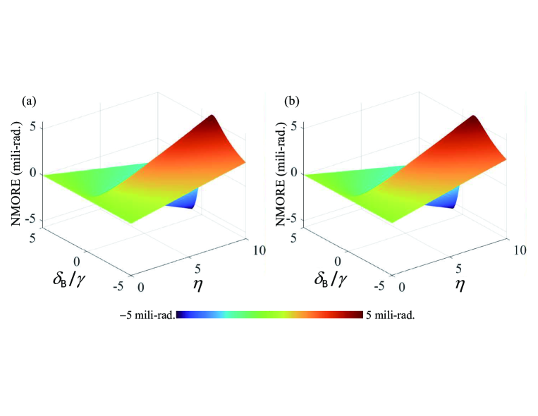
Figure 2: (a) Numerical solution by solving Eqs. (4a) and (4b) simultaneously. (b) NMORE evaluated using Eq. (6) by MATLAB. Parameters: $S_{0}=5$, $d_{2}=-5$, $\Delta_{0}=2$, $\kappa_{4}/\kappa_{2}=2$ ($\kappa_{2}=10^{5}$/cm.s), and $C_{0}=1.06$.

When the power broadening terms $\left(\frac{\Gamma_{0}S_{0}}{2}\right)$ in ${\cal M}_{m}$ ($m=1,..,4$) are neglected, we have ${\cal M}_{1}\rightarrow 1$, ${\cal M}_{2}\rightarrow e^{-2\alpha\eta}$, ${\cal M}_{3}\rightarrow 1$, and ${\cal M}_{4}\rightarrow 1$. Consequently, Eq. (6) gives

$$\Theta(\eta;d_{B})_{{}_{\rm NMORE}}\approx-\frac{\alpha d_{B}}{2(1+d_{B}^{2})}\Gamma_{0}S_{0}e^{-\alpha\eta}\eta,$$ (8)

which is the NMORE for a four-level single-probe AM with power broadening neglected but linear absorption included r15 . When the state $|4\rangle$ is neglected, $\alpha=\alpha_{2}$, $\Gamma_{0}=1/(1+d_{2}^{2})$, and we recover the NMORE of a three-level single-probe AM without power broadening. Equations (5) and (6) are the most accurate approximated analytical solution to NMORE of three and four-state systems to date. The validity and accuracy of Eqs. (5) and (6) have been thoroughly verified using a 4th order Runge-Kutta numerical differential equation solver on MATLAB, as well as a MATHEMATICA symbolic evaluation routine for broad probe power and detuning ranges r19 .

Figure 2(a) shows the NMORE of a four-state single-probe system obtained by a 4th order Runge-Kutta code that simultaneously solves Eqs. (4a) and (4b). Figure 2(b) shows the NMORE evaluated using Eq. (6) with the same parameters. The small difference validates the proposal of replacing $S_{\pm}(\eta)\rightarrow(S_{0}/2)e^{-\alpha\eta}$ in ${\cal P}_{\pm}$ and ${\cal Q}_{\pm}$. When the numerical and the approximated analytical solutions are plotted at $\eta=10$ as a function of $d_{B}$ we have found that with $C_{0}=1.05\pm 0.02$ excellent agreement between the two methods in a broad probe detuning and power regions [also see Fig. 3], a testimonial of the accuracy of Eq. (6).

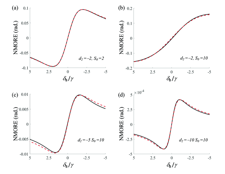
Figure 3: NMORE line profiles at $\eta=10$ by Eqs. (4a) and (4b) (black) and Eq. (6) (red). Figs. 3(a) and 3(b): $d_{2}=-2$ and probe powers are $S_{0}$=2 and 10, respectively. Here, a single amplitude adjustment constant $C_{0}=1.17$ is used for Eq. (6). Figs. 3(c) and 3(d): $S_{0}$=10 and probe detunings are $-5$ and $-10$, respectively, with $C_{0}=1.15\pm 0.02$ is used in Eq. (6).

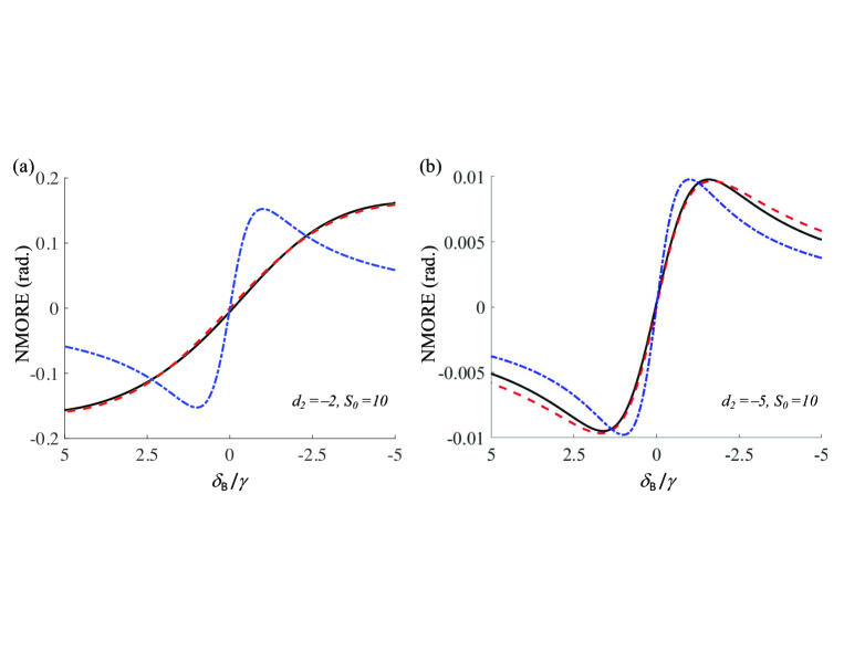
Figure 4: NMORE profiles obtained by numerical solution of Eqs. (4a) and (4b) (black), solutions from Eq. (6) (red) and Eq. (8) (blue) using $S_{0}=10$ and $\kappa_{4}/\kappa_{2}=2$. Probe detunings are (a): $d_{2}=-2$. (b): $d_{2}=-5$. For large detunings, three results are indistinguishable.

Figures 3(a)-3(d) show comparisons of numerical solutions with approximate analytical solutions for different probe powers and detunings. When $\kappa_{4}/\kappa_{2}=1$ the analytical solution achieves excellent agreement with the numerical solution in wide ranges of probe power and detuning for $C_{0}=1.00\pm 0.03$. When $\kappa_{4}/\kappa_{2}=2$, $d_{2}=-2$ we obtain remarkably accurate agreements in the probe power range of $S_{0}=$2 to 10 for a single amplitude adjustment constant of $C_{0}=1.17\pm 0.01$. For a fixed probe power of $S_{0}=10$, excellent agreements are obtained for a range of probe detuning $d_{2}$ from $-2$ to $-10$ with $C_{0}=1.15\pm 0.02$ r21 . Notice that the approximate analytical solution (red) show a slightly broader lineshape than the numerical solution (black). This is precisely because the replacement slightly overestimates the power-broadened line width.

It is quite remarkable that accurate results from Eq. (6) can be obtained in such a tight range of amplitude adjustment constant $C_{0}$ for broad ranges of laser power and detuning. Indeed, with laser power varying from $S_{0}=$2 to 10 and in the probe detuning range of $d_{2}=-2$ to $-10$, Eq. (6) yields accurate results that are all within $\pm 5\%$ of that by the full numerical calculations. Figure 4 compares the numerical solution [Eqs. (4a) and (4b), solid black], analytical solution (Eq. (6), dashed red) and the simplified solution (Eq. (8), dash-dotted blue). For small probe detuning, which is the necessary operation condition for a single-probe scheme reported in r7 , the simplified solution without power broadening does not agree with neither numerical solution nor the approximated analytical solution [Fig. (4a)]. However, when the probe detuning increases, all three methods approach the same result. We note that even though a small probe detuning r7 enhances NMORE signal amplitude, the power broadened lineshape leads to a significant reduction in magnetic field detection sensitivity (i.e., much smaller slope near zero field). With a large probe detuning, the detection sensitivity is preserved but the NMORE signal amplitude is reduced significantly [Fig. 4(b)]. The recently reported colliding-probe bi-atomic magnetometer experiments and theory r15a ; r15 overcome these issues, exhibiting excellent NMORE SNR, as well as increased field detection sensitivity at body temperature.

In conclusion, we have obtained the most accurate approximated analytical solutions to date for NMOREs of three and four-state systems with both probe absorption and power broadening. When the probe power broadening is neglected, we recover the known single-probe three and four-state system NMOREs. These general analytical solutions allow one to analyze multi-state magneto-optical rotation processes with excellent accuracy, revealing detailed effects and impacts of laser detuning, atomic hyper-fine splitting, as well as the probe power broadening on NMORE signal strength and magnetic field detection sensitivity.

Acknowledgments Claire Deng thanks Dr. Changfeng Fang (SDU) for technical assistance on MATLAB coding. LD acknowledges the financial support from SDU.

References

(1) D. Budker, W. Gawlik, D.F. Kimball, S.M. Rochester, V.V. Yashchuk, and A. Weis, ”Resonant nonlinear magneto-optical effects in atoms,” Rev. Mod. Phys. 74, 1153 (2002).
(2) A. Weis, J. Wurster, and S. I. Kanorsky, ”Quantitative interpretation of the nonlinear Faraday effect as a Hanle effect of a light-induced bi-refringence,” J. Opt. Soc. Am. B 10, 716-724 (1993).
(3) D. Budker and D.F.J. Kimball, ”Optical Magnetometry.” Cambridge University Press (2013).
(4) A.K. Zvezdin and V.A. Kotov, ”Modern Magneto-optics and Magneto-optical Materials,” Taylor & Francis Group, New York (1997).
(5) W. Gawlik and S. Pustelny, ”Nonlinear Magneto-Optical Rotation Magnetometers, High Sensitivity Magnetometers,” A. Grosz, M. J. Haji-sheikh, and S. C. Mukhopadhyay, Editors, Springer Series: Smart Sensors, Measurement and Instrumentation 19, 425-450, Springer International Publishing Switzerland 2017.
(6) M.O. Scully and M. Fleischhauer, ”High-sensitivity magnetometer based on index-enhanced media,” Phys. Rev. Lett. 69, 1360-1363 (1992).
(7) D. Budker, V. Yashchuk, and M. Zolotorev, ”Nonlinear magneto-optical effects with ultranarrow widths,” Phys. Rev. Lett. 81, 5788-5791 (1998)
(8) E.B. Aleksandrov et al., ”Laser pumping in the scheme of an Mx-magnetometer,” Optics Spectrosc. 78, 292-298 (1995).
(9) W. Happer and A.C. Tam, ”Effect of rapid spin exchange on the magnetic-resonance spectrum of alkali vapors,” Phys. Rev. A 16, 1877-1891 (1977).
(10) C.J. Erickson, D. Levron, W. Happer, S. Kadlecek, B. Chann, L.W. Anderson, T.G. Walker, ”Spin relaxation resonances due to the spin-axis interaction in dense rubidium and cesium vapors,” Phys. Rev. Lett. 85, 4237-4240 (2000).
(11) S. Kadlecek, L.W. Anderson, T.G. Walker, ”Field dependence of spin relaxation in a dense Rb vapor,” Phys. Rev. Lett. 80, 5512-5515 (1998).
(12) J.C. Allred, R.N. Lyman, T.W. Kornack, and M.V. Romalis, ”High-Sensitivity Atomic Magnetometer Unaffected by Spin-Exchange Relaxation,” Phys. Rev. Lett. 89, 130801 1-4 (2002).
(13) M.V. Balabas, T. Karaulanov, M.P. Ledbetter, and D. Budker, ”Polarized Alkali-Metal Vapor with Minute-Long Transverse Spin-Relaxation Time,” Phys. Rev. Lett. 105, 070801 1-4 (2010).
(14) A. Korver, R. Wyllie, B. Lancor, and T. G. Walker, ”Suppression of Spin-Exchange Relaxation Using Pulsed Parametric Resonance,” Phys. Rev. Lett. 111, 043002 (2013).
(15) F. Zhou, C. J. Zhu, E. W. Hagley, and L. Deng, ”Symmetry-breaking inelastic wave-mixing atomic magnetometry,” Sci. Adv. 3, e1700422 (2017).
(16) L. Deng, ”Colliding-probe bi-atomic magnetometers via energy circulation”, Photonics Research (submitted).
(17) Y.R. Shen, ”The Principles of Nonlinear Optics,” John Wiley & Sons, Chapters 9 and 10, New York 1984.
(18) This is because frequency shifts cancels out in the calculations of NMORE which is the difference between the phase of two probe components. We verified this by comparing numerical calculations with and without -dependent terms.
(19) In fact, most if not all warm vapor single-probe magnetometers fall in this category.
(20) For a 10-cm cell the probe field change is limited to only a few percent due to the single-probe-based NMORE blockade.
(21) For warm vapor experiments such as reported in Ref.r7 with sophisticated 5-layer magnetic shielding and RF modulation technique the laser is typically detuning by about =500 MHz (only about 1.5 Doppler linewidth) from states. Since Rubidium hyper-fine splitting is =820 MHz, which is about 2 Doppler linewidths, we therefore chose =2 in unit of .
(22) For instance, we first choose in Eq. (6) to obtained excellent agreement with numerical calculations for . Then, with a very narrow range of excellent agreements with numerical calculations can be obtained for the entire detuning range from to .