Sensitivity limits on the weak dipole moments of the top-quark at the Bestest Little Higgs Model

Abstract

We presented new researches for the sensitivity limits on the weak dipole moments of the top quark-$Z$ boson interactions in the context of the Bestest Little Higgs Model (BLHM). For this purpose, we derive the corresponding Feynman rules. Among the new contributions, there are those arising from the vertices of scalar bosons, vector bosons and heavy quarks contribution: $tq_{i}S_{i}$, ($S_{i}=h_{0},H_{0},A_{0},\phi^{0},\eta^{0},\sigma,H^{\pm},\phi^{\pm},\eta^{\pm}$); $tq_{i}V_{i}$, ($V_{i}=\gamma,Z,W,Z^{\prime},W^{\prime}$); and $Zq_{i}\bar{q}_{i}$ ($q_{i}=b,t,B,T,T_{5},T_{6},T^{2/3},T^{5/3}$). With these new vertices, we calculate the one-loop contributions to the weak dipole moments $a^{W}_{t}$ and $d^{W}_{t}$ of the top-quark in several scenarios. We found that with the parameters of the BLHM of $m_{A_{0}}=1000$ GeV, $m_{\eta^{0}}=100$ GeV, $F=4000$ GeV, $f=[1000,3000]$ GeV and $\tan\beta=3$, the $a^{W}_{t}$ reaches values with a sensitivity of $a^{W}_{t}=2.49\times 10^{-4}-1.26\times 10^{-5}i$, $1.26\times 10^{-4}-5.41\times 10^{-6}i$, where the main contribution comes from the scalars $h_{0}$ and $H_{0}$, which couples to the top-quark of the Standard Model and the top-quarks of the BLHM. These values seem to be out of the reach of the expected experimental sensitivity of present experiments. However, experiments on future colliders are expected to be sensitive enough to measure the AWMDM of the top-quark. Our study complements other studies at the level of one-loop with an extended scalar sector.

I Introduction

The top-quark with $m_{t}=172.76\pm 0.30$ GeV Data2020 is the most massive of all observed elementary particles in the Standard Model (SM). The large top-quark mass corresponds to a Yukawa coupling to the Higgs boson close to unity. This suggests that the top-quark may play a special role within the SM and that its precise characterization may shed light on the electroweak symmetry breaking mechanism PRL81-1998 ; PRD59-1999 . Because of the top-quark large mass, its couplings are expected to be more sensitive to new physics Beyond the SM (BSM) with respect to other particles Cao:2020npb . New physics can manifest itself in different forms. One possibility is that the new physics may lead to the appearance or a huge increase of new types of interactions like $tH^{+}b$ or anomalous Flavor Changing Neutral Current $tqg$, $tq\gamma$ and $tqZ$ ($q=u,c$) interactions. Another possibility is the modification of the SM couplings that involve $t\bar{t}\gamma$, $t\bar{t}Z$, $t\bar{t}g$ and $tWb$ vertices.

The top-quark is a key particle in various extensions BSM and is considered a laboratory for many experimental or simulation aspects in searches for new physics. In particular, the top-quark anomalous couplings to bosons in the $t\bar{t}\gamma$ and $t\bar{t}Z$ vertices, have made the top-quark one of the most attractive particles for new physics searches. In this regard, the study of the physics of the $t$-quark by the Tevatron collider at the Fermilab PLB713-2012 ; PLB693-2010 ; PRL102-2009 and the ATLAS and CMS Collaborations ATLAS-CONF-2012-126 ; PRL110-2013 ; EPJC79-2019 ; JHEP03-2020 ; Data2020 at the Large Hadron Collider (LHC) has been developed significantly in recent years and now represents a very active physics program.

One aspect of top-quark physics which is far less explored is interactions with neutral electroweak gauge bosons and the Higgs boson. The study of anomalous couplings in electroweak corrections is relatively unexplored, and therefore more detailed studies are warranted. Sensitivity to these couplings arises in hadronic collisions through the partonic subprocess $q\bar{q}\to(Z,\gamma)\to t\bar{t}$. At the LHC the $Z$ mediated process is overwhelmed by the strong production mechanism, rendering the tree level sensitivity vanishingly small. Electroweak loop corrections are another possible source of sensitivity to anomalous couplings.

Currently, little is known about anomalous couplings of the top-quark with the $Z$ boson. There are no direct measurements of these couplings; indirect measurements, using LEP and SLC data, tightly constrain only the $t\bar{t}Z$ vector and axial- vector couplings. On the other hand, the measurement of the $t\bar{t}Z$ production cross-section at the LHC ATLAS-CONF-2012-126 ; PRL110-2013 ; EPJC79-2019 ; JHEP03-2020 ; Data2020 offers a direct test of anomalous $t\bar{t}Z$ couplings. The experimental detection of non-zero Anomalous Weak Magnetic Dipole Moment (AWMDM) or Weak Electric Dipole Moment (WEDM) of heavy fermions such as $\tau$, $b$, and $t$ at the current sensitivity of the LHC, would be clear evidence of new physics BSM.

With these motivations, we carried out a study on the weak dipole moments of the quark-top in the context of the Bestest Little Higgs Model (BLHM) JHEP09-2010 . The purpose of the BLHM is to solve the hierarchy problem without fine-tuning. This is achieved through the incorporation of one-loop corrections to the Higgs boson mass through heavy top-quarks partners and heavy gauge bosons. This extension of the SM predicts the existence of new physical scalar bosons neutral and charged $h_{0},H_{0},A_{0},\phi^{0},\eta^{0},\sigma,H^{\pm},\phi^{\pm},\eta^{\pm}$, new heavy gauge bosons $Z^{\prime},W^{\prime}$ and new heavy quarks $B,T,T_{5},T_{6},T^{2/3},T^{5/3}$. At the one-loop level, the AWMDM $a^{W}_{t}$ and WEDM $d^{W}_{t}$ of the top-quark are induced via the Feynman diagrams depicted in Fig. 1, where $S_{i}$ represent scalar bosons, $V_{i}$ neutral and charged gauge bosons and $q_{i}$ heavy quarks. Therefore, among the new contributions of the model, there are those arising from the vertices of scalars bosons, vector bosons and heavy quarks contribution, that is to say, vertices of the form: $tq_{i}S_{i}$, $S_{i}=h_{0},H_{0},A_{0},\phi^{0},\eta^{0},\sigma,H^{\pm},\phi^{\pm},\eta^{\pm}$, $tq_{i}V_{i}$, $V_{i}=\gamma,Z,W,Z^{\prime},W^{\prime}$, and $Zq_{i}\bar{q}_{i}$, $q_{i}=b,t,B,T,T_{5},T_{6},T^{2/3},T^{5/3}$, respectively. With these vertices we calculate the one-loop contributions to the weak dipole moments $a^{W}_{t}$ and $d^{W}_{t}$ of the top-quark and in several scenarios with $m_{A_{0}}=1000,1500$ GeV, $m_{\eta^{0}}=100,500$ GeV, $F=[3000,6000]$ GeV, $f=[1000,3000]$ GeV and $\tan\beta=3$.

The paper is structured as follows. In Section II, we give a brief review of the BLHM. In Section III, we present the predictions of the BLHM on the weak dipole moments of the top-quark $a^{W}_{t}$ and $d^{W}_{t}$. Finally, we present our conclusions in Section IV. In Appendix A, we present the complete set of Feynman rules for the study of the weak dipole moments of the top-quark in the context of the BLHM. In Appendix B, we provide all the numerical contributions of the particles that induce the AWMDM of the top-quark.

II Brief review of the Bestest Little Higgs Model

Various extensions of the SM have been proposed in order to solve the problem of the mass hierarchy. One of the proposed extensions is the Little Higgs models (LHM) Arkani1 ; Arkani2 that employ a mechanism named collective symmetry breaking. Its main idea is to represent the SM Higgs boson as a pseudo-Nambu-Goldstone boson of an approximate global symmetry which is spontaneously broken at a scale in the TeV range. In these models, the collective symmetry breaking mechanisms is implemented in the norm sector, fermion sector and the Higgs sector, which predict new particles within the mass range of a few TeV. These new particles play the role of partners of the top-quark, of the gauge bosons and the Higgs boson, the effect of which is to generate radiative corrections for the mass of the Higgs boson, and thus cancel the divergent corrections induced by SM particles. LHM Arkani1 ; Arkani2 ; Arkani3 on the other hand already have strong constraints from electroweak precision data. These constraints typically require the new gauge bosons of LHM to be quite heavy PRD67-2003 ; PRD68-2003 . In most LHM, the top partners are heavier than the new gauge bosons, and this can lead to significant fine-tuning in the Higgs potential JHEP03-2005 .

An interesting and relatively recent model is the BLHM JHEP09-2010 overcomes these difficulties by including separate symmetry breaking scales at which the heavy gauge boson and top partners obtain their masses. This model features a custodial $SU(2)$ symmetry Schmaltz:2008vd ; Diaz:2001yz , has heavy gauge boson partner masses above the already excluded mass range, and has relatively light top partners below the upper bound from fine-tuning. The BLHM is based on two independent non-linear sigma models. With the first field $\Sigma$, the global symmetry $SO(6)_{A}\times SO(6)_{B}$ is broken to the diagonal group $SO(6)_{V}$ at the energy scale $f$, while with the second field $\Delta$, the global symmetry $SU(2)_{C}\times SU(2)_{D}$ to the diagonal subgroup $SU(2)$ to the scale $F>f$. In the first stage are generated 15 pseudo-Nambu-Goldstone bosons that are parameterized as

$$\Sigma=e^{i\Pi/f}e^{2i\Pi_{h}/f}e^{i\Pi/f},$$ (1)

where $\Pi$ and $\Pi_{h}$ are complex and antisymmetric matrices given by

$$\Pi=\left(\begin{array}[]{c c c}i(\phi_{a}T^{a}_{L}+\eta_{a}T_{R}^{a})_{4\times 4}&0&0\\ 0&0&i\sigma/\sqrt{2}\\ 0&-i\sigma/\sqrt{2}&0\end{array}\right),\hskip 28.45274pt\Pi_{h}=\frac{i}{\sqrt{2}}\left(\begin{array}[]{c c c}0_{4\times 4}&h_{1}&h_{2}\\ -h_{1}^{T}&0&0\\ -h_{2}^{T}&0&0\end{array}\right),$$ (8)

where $\phi_{a}$ and $\eta_{a}$ ($a=1,2,3$) are real triplets, $h_{1}$ and $h_{2}$ Higgs vectors as $\bf{4}^{\prime}$s of $SO(4)$, and $\sigma$ a real singlet. For Higgs fields, their explicit representation is $h_{i}^{T}=(h_{i1},h_{i2},h_{i3},h_{i4})$, while $T^{a}_{L,R}$ denote the generators of the group $SO(6)$ which are provided in JHEP09-2010 .

Regarding the second stage of spontaneous symmetry-breaking, the pseudo-Nambu-Goldstone bosons of the field $\Delta$ are parameterized as follows

$$\Delta=Fe^{2i\Pi_{d}/F},\,\,\,\,\,\Pi_{d}=\chi_{a}\frac{\tau^{a}}{2}\ \ (a=1,2,3),$$ (9)

where $\chi_{a}$ represents the Nambu-Goldstone fields and the $\tau_{a}$ correspond to the Pauli matrices, which are the generators of the SU(2) group.

II.1 The scalar sector

The BLHM Higgs fields, $h_{1}$ and $h_{2}$, form the Higgs potential that undergoes spontaneous symmetry-breaking JHEP09-2010 ; Kalyniak ; Erikson :

$$V_{Higgs}=\frac{1}{2}m_{1}^{2}h^{T}_{1}h_{1}+\frac{1}{2}m_{2}^{2}h^{T}_{2}h_{2}-B_{\mu}h^{T}_{1}h_{2}+\frac{\lambda_{0}}{2}(h^{T}_{1}h_{2})^{2}.$$ (10)

The potential reaches a minimum when $m_{1},m_{2}>0$, while the spontaneous electroweak symmetry-breaking requires that $B_{\mu}>m_{1}m_{2}$. The symmetry-breaking mechanism is implemented in the BLHM when the Higgs doublets acquire their vacuum expectation values (VEVs), $\langle h_{1}\rangle^{T}=(v_{1},0,0,0)$ and $\langle h_{2}\rangle^{T}=(v_{2},0,0,0)$. By demanding that these VEVs minimize the Higgs potential of Eq. (4), the following relations are obtained

$$v^{2}_{1}=\frac{1}{\lambda_{0}}\frac{m_{2}}{m_{1}}(B_{\mu}-m_{1}m_{2}),$$ (11)

$$v^{2}_{2}=\frac{1}{\lambda_{0}}\frac{m_{1}}{m_{2}}(B_{\mu}-m_{1}m_{2}).$$ (12)

These parameters can be expressed as follows

$$v^{2}\equiv v^{2}_{1}+v^{2}_{2}=\frac{1}{\lambda_{0}}\left(\frac{m^{2}_{1}+m^{2}_{2}}{m_{1}m_{2}}\right)\left(B_{\mu}-m_{1}m_{2}\right)\simeq\left(246\ \ \text{GeV}\right)^{2},$$ (13)

$$\text{tan}\,\beta=\frac{v_{1}}{v_{2}}=\frac{m_{2}}{m_{1}}.$$ (14)

From the diagonalization of the mass matrix for the scalar sector, three non-physical fields $G_{0}$ and $G^{\pm}$, two physical scalar fields $H^{\pm}$ and three neutral physical scalar fields $h_{0}$, $H_{0}$ and $A_{0}$ are generated Kalyniak ; PhenomenologyBLH . The lightest state, $h_{0}$, is identified as the scalar boson of the SM. The masses of these fields are given as

$$m_{G_{0}} = m_{G^{\pm}}=0,$$ (15)

$$m^{2}_{A_{0}} = m^{2}_{H^{\pm}}=m^{2}_{1}+m^{2}_{2},$$ (16)

$$m^{2}_{h_{0},H_{0}} = \frac{B_{\mu}}{\text{sin}\,2\beta}\mp\sqrt{\frac{B^{2}_{\mu}}{\text{sin}^{2}\,2\beta}-2\lambda_{0}B_{\mu}v^{2}\text{sin}\,2\beta+\lambda^{2}_{0}v^{4}\text{sin}^{2}\,2\beta}.$$ (17)

The four parameters present in the Higgs potential $m_{1},m_{2},B_{\mu}$ and $\lambda_{0}$, can be replaced by another more phenomenologically accessible set. That is, the masses of the states $h_{0}$ and $A_{0}$, the angle $\beta$ and the VEV $v$ Kalyniak :

$$B_{\mu} = \frac{1}{2}(\lambda_{0}v^{2}+m^{2}_{A_{0}})\,\text{sin}\,2\beta,$$ (18)

$$\lambda_{0} = \frac{m^{2}_{h_{0}}}{v^{2}}\Big{(}\frac{m^{2}_{h_{0}}-m^{2}_{A_{0}}}{m^{2}_{h_{0}}-m^{2}_{A_{0}}\text{sin}^{2}\,2\beta}\Big{)},$$ (19)

$$\text{tan}\,\alpha = \frac{B_{\mu}\text{cot}\,2\beta+\sqrt{(B^{2}_{\mu}/\text{sin}^{2}\,2\beta)-2\lambda_{0}B_{\mu}v^{2}\text{sin}\,2\beta+\lambda^{2}_{0}v^{4}\text{sin}^{2}\,2\beta}}{B_{\mu}-\lambda_{0}v^{2}\text{sin}\,2\beta},$$ (20)

$$m^{2}_{H_{0}} = \frac{B_{\mu}}{\text{sin}\,2\beta}+\sqrt{\frac{B^{2}_{\mu}}{\text{sin}^{2}\,2\beta}-2\lambda_{0}B_{\mu}v^{2}\text{sin}\,2\beta+\lambda^{2}_{0}v^{4}\text{sin}^{2}\,2\beta},$$ (21)

$$m^{2}_{\sigma} = (\lambda_{56}+\lambda_{65})f^{2}=2\lambda_{0}f^{2}\text{K}_{\sigma}.$$ (22)

From Eq. (22), the variables $\lambda_{56}$ and $\lambda_{65}$ represent the coefficients of the quartic potential defined in JHEP09-2010 , both variables take values different from zero to achieve the collective breaking of the symmetry and generate a quartic coupling of the Higgs boson Kalyniak . The BLHM also contains scalar triplet fields that get a contribution to their mass from the explicit symmetry breaking terms in model, as define in Ref. JHEP09-2010 , that depends on the parameter $m_{4}$.

$$m^{2}_{\phi^{0}} = \frac{16}{3}F^{2}\frac{3g^{2}_{A}g^{2}_{B}}{32\pi^{2}}\log\left(\frac{\Lambda^{2}}{m^{2}_{W^{\prime}}}\right)+m^{2}_{4}\frac{f^{4}+F^{4}}{F^{2}(f^{2}+F^{2})},$$ (23)

$$m^{2}_{\phi^{\pm}} = \frac{16}{3}F^{2}\frac{3g^{2}_{A}g^{2}_{B}}{32\pi^{2}}\log\left(\frac{\Lambda^{2}}{m^{2}_{W^{\prime}}}\right)+m^{2}_{4}\frac{f^{4}+f^{2}F^{2}+F^{4}}{F^{2}(f^{2}+F^{2})},$$ (24)

$$m^{2}_{\eta^{\pm}} = m^{2}_{4}+\frac{3f^{2}g^{2}_{Y}}{64\pi^{2}}\frac{\Lambda^{2}}{F^{2}},$$ (25)

$$m^{2}_{\eta^{0}} = m^{2}_{4}.$$ (26)

II.2 The gauge sector

In the BLHM the new gauge bosons develop masses proportional to $\sqrt{f^{2}+F^{2}}\sim F$. This makes the masses of the bosons large relative to other particles that have masses proportional to $f$. The kinetic terms of the gauge fields in the BLHM are given as follows:

$$\mathcal{L}=\frac{f^{2}}{8}\text{Tr}(D_{\mu}\Sigma^{\dagger}D^{\mu}\Sigma)+\frac{F^{2}}{4}\text{Tr}(D_{\mu}\Delta^{\dagger}D^{\mu}\Delta),$$ (27)

where

$$D_{\mu}\Sigma = \partial_{\mu}\Sigma+ig_{A}A^{a}_{1\mu}T^{a}_{L}\Sigma-ig_{B}\Sigma A^{a}_{2\mu}T^{a}_{L}+ig_{Y}B^{3}_{\mu}(T^{3}_{R}\Sigma-\Sigma T^{3}_{R}),$$ (28)

$$D_{\mu}\Delta = \partial_{\mu}\Delta+ig_{A}A^{a}_{1\mu}\frac{\tau^{a}}{2}\Delta-ig_{B}\Delta A^{a}_{2\mu}\frac{\tau^{a}}{2}.$$ (29)

$T^{a}_{L}$ are the generators of the group $SO(6)_{A}$ corresponding to the subgroup $SU(2)_{LA}$, while $T^{3}_{R}$ represents the third component of the $SO(6)_{B}$ generators corresponding to the $SU(2)_{LB}$ subgroup, these matrices are provided in JHEP09-2010 . $g_{A}$ and $A^{a}_{1\mu}$ denote the gauge coupling and field associated with the gauge bosons of $SU(2)_{LA}$. $g_{B}$ and $A^{a}_{2\mu}$ represent the gauge coupling and the field associated with $SU(2)_{LB}$, while $g_{Y}$ and $B^{3}_{\mu}$ denote the hypercharge and the field.

When $\Sigma$ and $\Delta$ get their VEVs, the gauge fields $A^{a}_{1\mu}$ and $A^{a}_{2\mu}$ are mixed to form a massless triplet $A^{a}_{0\mu}$ and a massive triplet $A^{a}_{H\mu}$,

$$A^{a}_{0\mu}=\text{cos}\,\theta_{g}A^{a}_{1\mu}+\text{sin}\,\theta_{g}A^{a}_{2\mu},\hskip 14.22636ptA^{a}_{H\mu}=\text{sin}\,\theta_{g}A^{a}_{1\mu}-\text{cos}\,\theta_{g}A^{a}_{2\mu},$$ (30)

with the mixing angles

$$s_{g}\equiv\sin\theta_{g}=\frac{g_{A}}{\sqrt{g_{A}^{2}+g_{B}^{2}}},\ \ c_{g}\equiv\cos\theta_{g}=\frac{g_{B}}{\sqrt{g_{A}^{2}+g_{B}^{2}}},$$ (31)

which are related to the electroweak gauge coupling $g$ through

$$\frac{1}{g^{2}}=\frac{1}{g^{2}_{A}}+\frac{1}{g^{2}_{B}}.$$ (32)

After the breaking of the electroweak symmetry, when the Higgs doublets, $h_{1}$ and $h_{2}$ acquire their VEVs, the masses of the gauge bosons of the BLHM are generated. In terms of the model parameters, the masses are given by

$$m^{2}_{\gamma} =0$$ , (33)

$$m^{2}_{Z} = \frac{1}{4}\left(g^{2}+g^{2}_{Y}\right)v^{2}\left(1-\frac{v^{2}}{12f^{2}}\left(2+\frac{3f^{2}}{f^{2}+F^{2}}\left(s^{2}_{g}-c^{2}_{g}\right)^{2}\right)\right),$$ (34)

$$m^{2}_{W} = \frac{1}{4}g^{2}v^{2}\left(1-\frac{v^{2}}{12f^{2}}\left(2+\frac{3f^{2}}{f^{2}+F^{2}}\left(s^{2}_{g}-c^{2}_{g}\right)^{2}\right)\right),$$ (35)

$$m^{2}_{Z^{\prime}} = m^{2}_{W^{\prime}}+\frac{g^{2}s^{2}_{W}v^{4}}{16c^{2}_{W}(f^{2}+F^{2})}\left(s^{2}_{g}-c^{2}_{g}\right)^{2},$$ (36)

$$m^{2}_{W^{\prime}} = \frac{g^{2}}{4c^{2}_{g}s^{2}_{g}}\left(f^{2}+F^{2}\right)-m^{2}_{W}.$$ (37)

The weak mixing angle is defined as

$$s_{W} \equiv\sin\theta_{W}=\frac{g_{Y}}{\sqrt{g^{2}+g^{2}_{Y}}},$$ (38)

$$c_{W} \equiv\cos\theta_{W}=\frac{g}{\sqrt{g^{2}+g^{2}_{Y}}},$$ (39)

$$x_{W} = \frac{1}{2c_{W}}s_{g}c_{g}(s^{2}_{g}-c^{2}_{g}).$$ (40)

II.3 The fermion sector

To construct the Yukawa interactions in the BLHM, the fermions must be transformed under the group $SO(6)_{A}$ or $SO(6)_{B}$. In this model, the fermion sector is divided into two parts. First, the sector of massive fermions is represented by Eq. (41). This sector includes the top and bottom quarks of the SM and a series of new heavy quarks arranged in four multiplets, $Q$, and $Q^{\prime}$ which transform under $SO(6)_{A}$, while $U^{c}$ and $U^{{}^{\prime}c}_{5}$ are transformed under the group $SO(6)_{B}$. Second, the sector of light fermions contained in Eq. (49), in this expression all the interactions of the remaining fermions of the SM with the exotic particles of the BLHM are generated.

For massive fermions, the Lagrangian that describes them is given by JHEP09-2010

$$\mathcal{L}_{t}=y_{1}fQ^{T}S\Sigma SU^{c}+y_{2}fQ^{\prime T}\Sigma U^{c}+y_{3}fQ^{T}\Sigma U^{\prime c}_{5}+y_{b}fq_{3}^{T}(-2iT^{2}_{R}\Sigma)U^{c}_{b}+H.c.,$$ (41)

where $S=\text{diag}(1,1,1,1,-1,-1)$. The multiplets are arranged as follows

$$Q^{T} = \frac{1}{\sqrt{2}}\left(\left(-Q_{a_{1}}-Q_{b_{2}}\right),i\left(Q_{a_{1}}-Q_{b_{2}}\right),\left(Q_{a_{2}}-Q_{b_{1}}\right),i\left(Q_{a_{2}}-Q_{b_{1}}\right),Q_{5},Q_{6}\right),$$ (42)

$$Q^{\prime T} = \frac{1}{\sqrt{2}}(-Q^{\prime}_{a_{1}},iQ^{\prime}_{a_{1}},Q^{\prime}_{a_{2}},iQ^{\prime}_{a_{2}},0,0),$$ (43)

$$q_{3}^{T} = \frac{1}{\sqrt{2}}(-\bar{t}_{L},i\bar{t}_{L},\bar{b}_{L},i\bar{b}_{L},0,0),$$ (44)

$$U^{cT} = \frac{1}{\sqrt{2}}\left((-U^{c}_{b_{1}}-U^{c}_{a_{2}}),i(U^{c}_{b_{1}}-U^{c}_{a_{2}}),(U^{c}_{b_{2}}-U^{c}_{a_{1}}),i(U^{c}_{b_{2}}-U^{c}_{a_{1}}),U^{c}_{5},U^{c}_{6}\right),$$ (45)

$$U^{\prime cT} = (0,0,0,0,U^{\prime c}_{5},0),$$ (46)

$$U_{b}^{cT} = (0,0,0,0,b^{c},0).$$ (47)

The explicit forms of the components of the multiplets are defined in Ref. JHEP09-2010 . For simplicity, the Yukawa couplings are assumed to be real $y_{1},y_{2},y_{3}$ $\in R$. The Yukawa coupling of the top-quark is defined as

$$y_{t}=\frac{3y_{1}y_{2}y_{3}}{\sqrt{(y^{2}_{1}+y^{2}_{2})(y^{2}_{1}+y^{2}_{3})}}=\frac{m_{t}}{v\sin\beta}.$$ (48)

For light fermions the corresponding Lagrangian is

$$\mathcal{L}_{light}=\sum_{i=1,2}y_{u}fq^{T}_{i}\Sigma u^{c}_{i}+\sum_{i=1,2}y_{d}fq^{T}_{i}(-2iT^{2}_{R}\Sigma)d^{c}_{i}+\sum_{i=1,2,3}y_{e}fl^{T}_{i}(-2iT^{2}_{R}\Sigma)e^{c}_{i}+h.c.,$$ (49)

with

$$q^{T}_{i} = \frac{1}{\sqrt{2}}(-\bar{u}_{iL},i\bar{u}_{iL},\bar{d}_{iL},i\bar{d}_{iL},0,0),$$ (50)

$$l^{T}_{i} = \frac{1}{\sqrt{2}}(-\bar{\nu}_{iL},i\bar{\nu}_{iL},\bar{e}_{iL},i\bar{e}_{iL},0,0),$$ (51)

$$u^{cT}_{i} = (0,0,0,0,u^{c}_{i},0),$$ (52)

$$d^{cT}_{i} = (0,0,0,0,d^{c}_{i},0),$$ (53)

$$e^{cT}_{i} = (0,0,0,0,e^{c}_{i},0).$$ (54)

After breaking the electroweak symmetry, the resulting mass terms are expanded by a power series up to $\frac{v^{2}}{f^{2}}$ and the mass matrices are diagonalized using perturbation theory. The fermion mass eigenstates are calculated under the assumption that $y_{2}\neq y_{3}$, otherwise the masses of $T$ and $T_{5}$ are degenerate at lowest order PhenomenologyBLH :

$$m^{2}_{t} = y^{2}_{t}v^{2}_{1},$$ (55)

$$m^{2}_{T} = (y^{2}_{1}+y^{2}_{2})f^{2}+\frac{9v^{2}_{1}y^{2}_{1}y^{2}_{2}y^{2}_{3}}{(y^{2}_{1}+y^{2}_{2})(y^{2}_{2}-y^{2}_{3})},$$ (56)

$$m^{2}_{T_{5}} = (y^{2}_{1}+y^{2}_{3})f^{2}-\frac{9v^{2}_{1}y^{2}_{1}y^{2}_{2}y^{2}_{3}}{(y^{2}_{1}+y^{2}_{3})(y^{2}_{2}-y^{2}_{3})},$$ (57)

$$m^{2}_{T_{6}} = m^{2}_{T^{2/3}_{b}}=m^{2}_{T^{5/3}_{b}}=y^{2}_{1}f^{2},$$ (58)

$$m^{2}_{B} = (y^{2}_{1}+y^{2}_{2})f^{2},$$ (59)

with $v_{1}=v\sin\beta$ y $v_{2}=v\cos\beta$.

II.4 The currents sector

In this sector the interactions of the fermions with the gauge bosons are determined. The vertices are obtained from the following Lagrangian PhenomenologyBLH ,

$$\mathcal{L} = \bar{Q}\bar{\tau}^{\mu}D_{\mu}Q+\bar{Q}^{\prime}\bar{\tau}^{\mu}D_{\mu}Q^{\prime}-U^{c\dagger}\tau^{\mu}D_{\mu}U^{c}-U^{\prime c\dagger}\tau^{\mu}D_{\mu}U^{\prime c}-U_{b}^{c\dagger}\tau^{\mu}D_{\mu}U_{b}^{c}+\sum_{i=1,2}q^{\dagger}_{i}\tau^{\mu}D_{\mu}q_{i}$$ (60)

$$+ \sum_{i=1,2,3}l^{\dagger}_{i}\tau^{\mu}D_{\mu}l_{i}-\sum_{i=1,2,3}e_{i}^{c\dagger}\tau^{\mu}D_{\mu}e^{c}_{i}-\sum_{i=1,2}u_{i}^{c\dagger}\tau^{\mu}D_{\mu}u^{c}_{i}-\sum_{i=1,2}d_{i}^{c\dagger}\tau^{\mu}D_{\mu}d^{c}_{i},$$

where $\tau^{\mu}$ and $\bar{\tau}^{\mu}$ are defined according to Spremier . The respective covariant derivatives are

$$D_{\mu}Q = \partial_{\mu}Q+\sum_{a}(ig_{A}A^{a}_{1\mu}T^{a}_{L}Q)+ig_{Y}B_{3\mu}(T^{3}_{R}+T^{+}_{X})Q,$$ (61)

$$D_{\mu}Q^{\prime} = \partial_{\mu}Q^{\prime}+\sum_{a}(ig_{A}A^{a}_{1\mu}T^{a}_{L}Q^{\prime})+ig_{Y}B_{3\mu}\left(\frac{1}{6}\right)Q^{\prime},$$ (62)

$$D_{\mu}U^{c} = \partial_{\mu}U^{c}+\sum_{a}(ig_{B}A^{a}_{2\mu}T^{a}_{L}U^{c})+ig_{Y}B_{3\mu}(T^{3}_{R}+T^{-}_{X})U^{c},$$ (63)

$$D_{\mu}U^{\prime c} = \partial_{\mu}U^{\prime c}+ig_{Y}B_{3\mu}T^{-}_{X}U^{\prime c},$$ (64)

$$D_{\mu}U_{b}^{c} = \partial_{\mu}U_{b}^{c}+ig_{Y}B_{3\mu}\left(\frac{1}{3}\right)U_{b}^{c},$$ (65)

$$D_{\mu}q_{i} = \partial_{\mu}q_{i}+\sum_{a}(ig_{A}A^{a}_{1\mu}T^{a}_{L}q_{i})+ig_{Y}B_{3\mu}(T^{3}_{R}+T^{+}_{X})q_{i},$$ (66)

$$D_{\mu}l_{i} = \partial_{\mu}l_{i}+\sum_{a}(ig_{B}A^{a}_{2\mu}T^{a}_{L}l_{i})+ig_{Y}B_{3\mu}T^{3}_{R}l_{i},$$ (67)

$$D_{\mu}e^{c}_{i} = \partial_{\mu}e_{i}^{c}+ig_{Y}B_{3\mu}T^{e}_{X}e^{c}_{i},$$ (68)

$$D_{\mu}u^{c}_{i} = \partial_{\mu}u_{i}^{c}+ig_{Y}B_{3\mu}T^{-}_{X}u^{c}_{i},$$ (69)

$$D_{\mu}d^{c}_{i} = \partial_{\mu}d_{i}^{c}+ig_{Y}B_{3\mu}T^{d}_{X}d^{c}_{i}.$$ (70)

The Feynman rules of the BLHM involved in our calculation are obtained by transforming the gauge eigenstate in terms of the mass eigenstates for the fermions, the gauge bosons, and the scalars bosons (see Appendix C of Ref. Martin:2012kqb ).

III Sensitivity limits on the AWMDM $a^{W}_{t}$ at the BLHM

The weak properties of the top-quark appear in the quantum field theory of its interaction with the $Z$ boson. In this regard, the most general Lorentz-invariant vertex function describing the interaction of a $Z$ boson with two top-quarks can be written in terms of ten form factors NPB551-1999 ; NPB812-2009 , which are functions of the kinematic invariants. In the low energy limit, these correspond to couplings that multiply dimension-four or-five operators in an effective Lagrangian, and may be complex. If the $Z$ boson couples to effectively massless fermions, the number of independent form factors is reduced to eight. In addition, if both top-quarks are on-shell, the number is further reduced to four. In this case, the $t\bar{t}Z$ vertex can be written in the form

$$ie\bar{u}(p^{\prime})\Gamma^{\mu}_{t\bar{t}Z}(q^{2})u(p) = ie\bar{u}(p^{\prime})\big{\{}\gamma^{\mu}\left[F_{V}(q^{2})-F_{A}(q^{2})\gamma^{5}\right]$$ (71)

$$+ i\sigma^{\mu\nu}q_{\nu}\left[F_{M}(q^{2})-iF_{E}(q^{2})\gamma^{5}\right]\big{\}}u(p),$$

where $e$ is the proton charge. The terms $F_{V}(0)$ and $F_{A}(0)$ in the low energy limit are the $t\bar{t}Z$ vector and axial-vector form factors in the SM, while $F_{M}(q^{2})$ and $F_{E}(q^{2})$ are associated with the form factors of the weak dipole moments. The latter appear due to quantum corrections and are a valuable tool to study the effects of new physics indirectly way, through virtual corrections of new particles predicted by extensions of the SM. Another characteristic of form factors is that they only depend on an independent dynamic variable, $q^{2}$, where $q=p-p^{\prime}$ and denotes the incoming moment of the $Z$ boson. In this work, the $Z$ boson is off-shell mass since to produce a top-quark pair the $Z$ must necessarily be off the resonance. For this case, the well-known gauge dependence problem arises and occurs when one studies the radiative corrections to fermion-pair production at colliders with center-of-mass energy beyond the mass of the $Z$ boson, that is, $\sqrt{q^{2}}>2m_{t}$ Bernabeu:1995gs . In this case, the pinch technique Papavassiliou:1993qe ; Cornwall:1989gv ; Cornwall:1981zr ; Alkofer:2000wg ; Papavassiliou:1996zn can be used to remove the gauge dependence. Our results are useful to determine the effects of new physics that could be potentially very important. With respect to form factors, $F_{M}(q^{2})$ and $F_{E}(q^{2})$, these are related to the AWMDM $a^{W}_{t}$ and the WEDM $d^{W}_{t}$:

$$F_{M}(q^{2}) = -\frac{a^{W}_{t}}{2m_{t}},$$ (72)

$$F_{E}(q^{2}) = -\frac{d^{W}_{t}}{e}.$$ (73)

It is worth mentioning that, the weak magnetic dipole form factor $F_{M}(q^{2})$ receives contributions at the one-loop level in the SM. However, there is no such contribution to the weak electric dipole form factor, $F_{E}(q^{2})$ NPB551-1999 . For this reason, we only estimate limits on the AWMDM of the top-quark.

III.1 Contribution of new scalar bosons, gauge bosons and heavy quarks to the AWMDM of the top-quark

The AWMDM of top-quark carries important information about interactions with other particles. Their small magnitude in the SM makes these couplings ideal for probing new physics interactions and for exploring the potential role of top-quark in electroweak symmetry breaking, which has yet to be elucidated. In this way, the top-quark is expected to be a window to any new physics at the TeV energy scale. In this subsection, we evaluated the AWMDM of the top-quark in the context of the BLHM. All the possible one-loop contributions to the $F_{M}(q^{2})$ and $F_{E}(q^{2})$ form factors can be classified in terms of the two classes of triangle diagrams depicted in Fig. 1. From this figure we can see that $S_{i}$, $V_{i}$ and $q_{i}$ are the particles circulating in the loop: $S_{i}$ represents the scalars $h_{0}$ (SM Higgs boson), $H_{0},A_{0},\phi^{0},\eta^{0},\sigma,H^{\pm},\phi^{\pm},\eta^{\pm}$; $V_{i}$ stands for the gauge bosons $\gamma,Z,W,Z^{\prime},W^{\prime}$; and $q_{i}$ denotes the quarks $b,t,B,T,T_{5},T_{6},T^{2/3},T^{5/3}$. To obtain the amplitude of each contribution we need to know the Feynman rules involved in the diagrams shown in Fig. 1, these vertices are provided in Appendix A.

In the unitary gauge, there are 52 diagrams that contribute to vertex $t\bar{t}Z$. We classify these contributions into two categories, which are written in the following compact form:

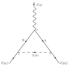
(a)

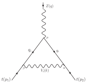
(b)

Figure 1: Feynman diagrams contributing to the AWMDM of the top-quark at one-loop. a) Scalar bosons $S_{i}=h_{0},H_{0},A_{0},\phi^{0},\eta^{0},\sigma,H^{\pm},\phi^{\pm},\eta^{\pm}$, b) Vector bosons $V_{i}=\gamma,Z,W,Z^{\prime},W^{\prime}$, and heavy quarks $q_{i}=b,t,B,T,T_{5},T_{6},T^{2/3},T^{5/3}$.

$$\mathcal{M}^{\mu}_{t}(S_{i}) = \int\frac{d^{4}k}{(2\pi)^{4}}\bar{u}(p_{2})\left(f^{*}_{S_{i}}+f^{*}_{P_{i}}\gamma^{5}\right)\left[i\frac{\not\!k+\not\!p_{2}+m_{q_{i}}}{(k+p_{2})^{2}-m^{2}_{q_{i}}}\right]\left(\gamma^{\mu}(F_{V_{i}}+F_{A_{i}}\gamma^{5})\right)$$ (74)

$$\times \left[i\frac{\not\!k+\not\!p_{1}+m_{q_{i}}}{(k+p_{1})^{2}-m^{2}_{q_{i}}}\right]\left(f_{S_{i}}+f_{P_{i}}\gamma^{5}\right)u(p_{1})\left(\frac{i}{k^{2}-m^{2}_{S_{i}}}\right),$$

$$\mathcal{M}^{\mu}_{t}(V_{i}) = \int\frac{d^{4}k}{(2\pi)^{4}}\bar{u}(p_{2})\gamma^{\alpha}\left(f^{*}_{V_{i}}+f^{*}_{A_{i}}\gamma^{5}\right)\left[i\frac{\not\!k+\not\!p_{2}+m_{q_{i}}}{(k+p_{2})^{2}-m^{2}_{q_{i}}}\right]\left(\gamma^{\mu}(F_{V_{i}}+F_{A_{i}}\gamma^{5})\right)$$ (75)

$$\times \left[i\frac{\not\!k+\not\!p_{1}+m_{q_{i}}}{(k+p_{1})^{2}-m^{2}_{q_{i}}}\right]\gamma^{\beta}\left(f_{V_{i}}+f_{A_{i}}\gamma^{5}\right)u(p_{1})\left[\frac{i}{k^{2}-m^{2}_{V_{i}}}\left(-g_{\alpha\beta}+\frac{k_{\alpha}k_{\beta}}{m^{2}_{V_{i}}}\right)\right],$$

where $f_{S_{i}},f_{P_{i}},f_{V_{i}}$ and $f_{A_{i}}$ denote the form factors of the scalars, pseudoscalar, vector and axial-vector. For the virtual photon case, the longitudinal term of the propagator in Eq. (75) is absent. For each amplitude we have to pick up only the coefficients of $\sigma^{\mu\nu}q_{\nu}$ and $\sigma^{\mu\nu}q_{\nu}\gamma^{5}$ shown in Eq. (71). Therefore, the contributions of the new physics to the AWMDM and WEDM of the top-quark are given as follows

$$a^{W}_{t}\equiv[a^{W}_{t}]^{BLHM} = [a^{W}_{t}]^{S_{i}}+[a^{W}_{t}]^{V_{i}},$$ (76)

$$d^{W}_{t}\equiv[d^{W}_{t}]^{BLHM} = [d^{W}_{t}]^{S_{i}}+[d^{W}_{t}]^{V_{i}}.$$ (77)

In the context of the BLHM, $d^{W}_{t}$ is absent so it does not receive radiative corrections at the one-loop level.

III.2 Parameters space

We consider the following input parameters: $m_{A_{0}}$, $m_{\eta_{0}}$ y $\tan\beta$. The mass of the pseudoscalar $A_{0}$, which is fixed around 1000 GeV, is in strict agreement with the most recent experimental data on searches for new scalar particles ATLAS:2020gxx . On the other hand, the free parameters $m_{4,5,6}$ JHEP09-2010 are introduced to break all the axial symmetries in the Higgs potential, giving positive masses to all scalars. Specifically, the $\eta_{0}$ scalar receives a mass equal to $m_{4}=m_{\eta_{0}}=100$ GeV, according to the BLHM, and the restriction $m_{4}\gtrsim 10$ GeV must be considered JHEP09-2010 . The following theoretical constraints on the BLHM parameters are imposed, primarily due to perturbativity requirements, such as the value of the mixing angle $\beta$, which is restricted to be

$$1<\text{tan}\ \beta<\sqrt{\frac{2+2\sqrt{\big{(}1-\frac{m^{2}_{h_{0}}}{m^{2}_{A_{0}}}\big{)}\big{(}1-\frac{m^{2}_{h_{0}}}{4\pi v^{2}}\big{)}}}{\frac{m^{2}_{h_{0}}}{m^{2}_{A_{0}}}\big{(}1+\frac{m^{2}_{A_{0}}-m^{2}_{h_{0}}}{4\pi v^{2}}\big{)}}-1}.$$ (78)

From this inequality we can extract values for the $\tan\beta$ parameter. In particular, for $m_{A_{0}}=1000$ GeV, it is obtained that $1<\tan\beta<10.45$. For our analysis we choose $\tan\beta=3$, $m_{A_{0}}=1000$ GeV, $m_{\eta_{0}}=100$ GeV and $F=4000$ GeV. Due to the characteristics of the BLHM, avoiding fine-tuning requires light exotic quarks whereas precision electroweak constraints require new heavy gauge bosons JHEP09-2010 . In this way, the energy scale $F$ was chosen to be large enough to ensure that the new gauge bosons are much heavier than the exotic quarks. Recall that the new heavy gauge bosons develop masses proportional to combination of $f$ and $F$ (see Eqs. (36) and (37)).

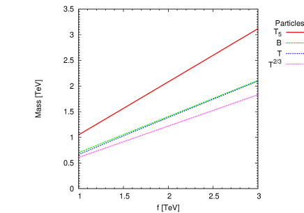
(a)

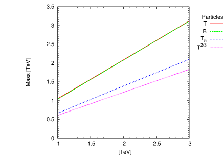
(b)

(c)

Figure 2: Behavior of particle masses as a function of the energy scale $f$ in the BLHM. a) Heavy quarks in the region $y_{2}<y_{3}$. b) Heavy quarks in the region $y_{2}>y_{3}$. c) Scalars and vector bosons.

In Fig. 2, we show the spectrum of the new particles whose masses are proportional to the energy scale $f$. As mentioned in the Subsection II.3, the analytical expressions for the mass eigenvalues, Eqs. (55) - (59), are valid only for the region $|y_{2}-y_{3}|>0$. In this way, the exotic quarks obey the following mass hierarchy in the corresponding sub-regions PhenomenologyBLH ; Godfrey:2012tf ,

$$y_{2}<y_{3},\ m_{T^{2/3}} = m_{T^{5/3}}=m_{T_{6}}<m_{T}<m_{B}<m_{T_{5}},$$ (79)

$$y_{2}>y_{3},m_{T^{2/3}} = m_{T^{5/3}}=m_{T_{6}}<m_{T_{5}}<m_{B}<m_{T}.$$ (80)

When $y_{2}<y_{3}$, the mass difference between the $T_{5}$ and $T_{6}$ quarks is large, this increases the decay modes available for the $T_{5}$ state through cascades decays to non-SM particles. While for $y_{2}>y_{3}$, the mass splitting between $T_{5}$ and $T_{6}$ is relatively small, so $T_{5}$ state decays predominantly to SM particles PhenomenologyBLH ; Godfrey:2012tf . Since the range of parameter space for this model is large, we restrict our study to two sample sub-regions of parameter space that characterize the range of mass for the new heavy quarks, for this purpose we choose: $y_{1}=0.61$, $y_{2}=0.35$, $y_{3}=0.84$ ($y_{2}<y_{3}$) and $y_{1}=0.61$, $y_{2}=0.84$, $y_{3}=0.35$ ( $y_{2}>y_{3}$). The values of the three Yukawa couplings are fixed through the top-quark mass (see Eq. (48)) and satisfy a perturbative scenario. Therefore, with these values of $y_{1,2,3}$ the masses for the heavy quarks are generated, these are provided in Eqs. (81) - (88). In the established scenarios, the lightest quarks are $T^{2/3}$, $T^{5/3}$ and $T_{6}$ as they acquire lower limits on their masses up to 610 GeV CMS:2018ubm ; CMS:2013wkd ; CDF:2009gat ; Contino:2008hi .

• Prediction with $y_{2}<y_{3}$:

  $$m_{T} = [663.3,2096.8]\ \text{GeV},$$ (81)

  $$m_{T_{5}} = [1050.1,3118.4]\ \text{GeV},$$ (82)

  $$m_{T^{2/3}} = m_{T^{5/3}}=m_{T_{6}}=[610.0,1830.0]\ \text{GeV},$$ (83)

  $$m_{B} = [703.3,2109.8]\ \text{GeV}.$$ (84)

• Prediction with $y_{2}>y_{3}$:

  $$m_{T} = [1050.1,3118.4]\ \text{GeV},$$ (85)

  $$m_{T_{5}} = [663.3,2096.8]\ \text{GeV},$$ (86)

  $$m_{T^{2/3}} = m_{T^{5/3}}=m_{T_{6}}=[610.0,1830.0]\ \text{GeV},$$ (87)

  $$m_{B} = [1038.1,3114.4]\ \text{GeV}.$$ (88)

With respect to the masses of the scalar and vector particles, in Fig. 2 (c) we observe that $\sigma$ is the heaviest scalar, while $\eta^{\pm}$ is the lightest one. The new gauge bosons $Z^{\prime}$ and $W^{\prime}$ acquire equal masses. Due to the fine-tuning constraints, the scale $f$ is varied from 1000 to 3000 GeV, thus obtaining a range of masses for each of the new quarks, scalar bosons, and vector bosons.

$$m_{\sigma} = [2108.7,6326.0]\ \text{GeV},$$ (89)

$$m_{\phi^{0}} = [722.3,975.7]\ \text{GeV},$$ (90)

$$m_{\eta^{\pm}} = [315.3,902.7]\ \text{GeV},$$ (91)

$$m_{\phi^{\pm}} = [722.5,976.7]\ \text{GeV},$$ (92)

$$m_{Z^{\prime}} = m_{W^{\prime}}=[3831.7,4225.9]\ \text{GeV}.$$ (93)

The masses of the scalars $H^{\pm}$ and $H_{0}$ do not depend on the energy scale $f$ but are calculated from the input parameters of the BLHM, $m_{A_{0}}$ and $\tan\beta$ (see Eqs. (16) and (21)).

$$m_{H^{\pm}} = m_{A_{0}},$$ (94)

$$m_{H_{0}} \approx 1010\ \text{GeV},\ \ \ \ \text{for}\ m_{A_{0}}=1000\ \text{GeV}.$$ (95)

III.3 Constraints on model parameters

The structure of the BLHM was constructed to solve some problems that occur in most Little Higgs models. The reason this model succeeds is that it is built under two separate symmetry-breaking scales, $f$ and $F>f$, at which the exotic quarks and heavy gauge bosons, respectively, obtain their masses. Thus, the gauge bosons are relatively heavy, consistent with electroweak precision measurements because masses above the already excluded mass range are generated. For the fermion sector of the model, the most stringent theoretical constraint on the masses of the exotic quarks comes from fine-tuning of the Higgs potential due to fermion loops. It is therefore important to determine realistic values of the three Yukawa couplings, $y_{1,2,3}$, and the top-quark Yukawa coupling, $y_{t}$, that evade the fine-tuning constraints. In this sense, a fit on the Yukawa coupling parameters is required. In the BLHM, the size of the fine-tuning can be computed in the following way JHEP09-2010 ; PhenomenologyBLH

$$\Psi=\frac{|\delta m^{2}_{1}|}{\lambda_{0}v^{2}\cos^{2}\beta},\ \delta m^{2}_{1}=-\frac{27f^{2}}{8\pi^{2}}\frac{y^{2}_{1}y^{2}_{2}y^{2}_{3}}{y^{2}_{2}-y^{2}_{3}}\,\text{log}\left(\frac{y^{2}_{1}+y^{2}_{2}}{y^{2}_{1}+y^{2}_{3}}\right).$$ (96)

If $\Psi\sim 1$, this indicates that there is no fine-tuning in the model. On the other hand, the top-quark Yukawa coupling is determined by

$$y_{t}=\frac{m_{t}}{v\sin\beta}=\frac{3y_{1}y_{2}y_{3}}{\sqrt{\left(y^{2}_{1}+y^{2}_{2}\right)\left(y^{2}_{1}+y^{2}_{3}\right)}},$$ (97)

where $m_{t}=172.76$ GeV is the top-quark mass, thus finding $y_{t}=0.74$. With this fixed value of $y_{t}$, we can randomize perturbative values for the $y_{1,2,3}$ parameters. In order to obtain a numerical estimate of the fine-tuning and an upper limit for the $f$ scale where the new physics does not significantly require fine-tuning, we choose the following values: $y_{1}=0.61$, $y_{2}=0.35$ and $y_{3}=0.84$, with $f<3100$ GeV. In this scenario we will carry out our analysis of the AWMDM of the top-quark, as for the $y_{2}>y_{3}$ scenario, this could be the subject of another study shortly soon EA . Finally, the gauge couplings $g_{A}$ and $g_{B}$, associated with the $SU(2)_{LA}$ and $SU(2)_{LB}$ gauge bosons, can be parametrized in a more phenomenological form in terms of a mixing angle $\theta_{g}$ and the $SU(2)_{L}$ gauge coupling: $\tan\theta_{g}=g_{A}/g_{B}$ and $g=g_{A}g_{B}/\sqrt{g^{2}_{A}+g^{2}_{B}}$. For simplicity, we can assume that $\tan\theta_{g}=1$, which implies that the gauge couplings $g_{A}$ and $g_{B}$ are equal. The $g_{A,B}$ values are generated using the restriction $g=0.6525$.

III.4 Feynman rules

In order to facilitate the phenomenological study of the weak dipole moments of the top-quark in the BLHM. We provide in Appendix A all the Feynman rules of the interaction vertices obtained in the unitary gauge. These three-point vertices refer to the couplings between gauge bosons and fermions, and scalars and fermions. The complete set of Feynman rules presented in this study was determined using perturbation theory and expanded up to $\mathcal{O}(\frac{1}{f^{2}})$.

III.5 The top-quark at the ILC

Top-quark production in the process $e^{+}e^{-}\rightarrow Z^{*}/\gamma\rightarrow t\bar{t}$ at the International Linear Collider (ILC) Behnke:2013xla ; Baer:2013cma ; Adolphsen:2013kya is a powerful tool to determine indirectly the scale of new physics. Such a machine offers several advantages over a hadron collider such as the LHC, especially in performing SM precision measurementes Baer:2013cma since it provides an experimentally clean environment without hadronic activity in the state initial, and the collision energy is accurately known. The ILC is designed to operate in phase II at a center-of-mass energy of $\sqrt{s}=500$ GeV, at this energy top-quark pairs are produced numerously well above threshold Cao:2015qta .

Thus, in order to give numerical results to $a^{W}_{t}$, we adopt the same collider parameters of the $e^{+}e^{-}$ linear collider, that is, $\sqrt{s}=\sqrt{q^{2}}=500$ GeV. Therefore, we have computed the contributions to the AWMDM $a^{W}_{t}$ of the on-shell top-quark with the $Z$ boson at the center-of-mass energy expected for the ILC. On the other hand, in this same scenario, it was obtained that the WEDM $d^{W}_{t}$ does not receive contributions to one-loop. In the SM, $d^{W}_{t}$ only receives contributions at three-loops Hollik:1998vz ; Czarnecki:1996rx .

III.6 Numerical results

To solve the integrals involved in the generic amplitudes, the Passarino-Veltman reduction scheme was implemented in the environment of the Mathematica Feyncalc Mertig:1990an and Package-X Patel:2015tea . The kinematic conditions were used in these packages, as well as the Gordon identity to eliminate the terms proportional to ($p_{1}+p_{2}$)^μ. After this, the AWMDM of the top-quark is obtained through the relation $a^{W}_{t}=-2m_{t}F_{M}(q^{2})$. In this study, we do not report the analytical expressions for $a^{W}_{t}$ because are very large expressions, for this reason, we only report our numerical results.

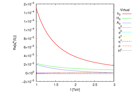
(a)

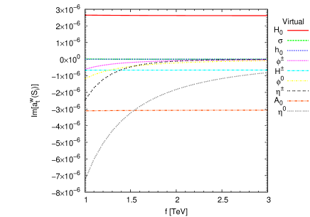
(b)

Figure 3: Individual scalar contributions to $a^{W}_{t}$ in the BLHM for fixed values of $m_{A_{0}}=1000\,\text{GeV}$, $m_{\eta^{0}}=100\,\text{GeV}$ and $F=4000\,\text{GeV}$. a) Re($a^{W}_{t}$). b) Im($a^{W}_{t}$).

From the 52 diagrams contributing to the $t\bar{t}Z$ vertex, we start by extracting the contributions to $a^{W}_{t}$ due to the different scalar bosons and vector bosons. In Figs. (3) - (4) is shown $a^{W}_{t}$ as a function of the new physics scale $f$ for the intervalo $f=[1000,3000]$ GeV. From Fig. 3 we can appreciate the individual contributions of the scalars involved, and we observe that the main contributions to the real and imaginary part of $a^{W}_{t}$ are generated by the Higgs bosons $h_{0}$ and $H_{0}$: $\text{Re}[a^{W}_{t}(h_{0})]=[1.51\times 10^{-4},1.70\times 10^{-5}]$ and $\text{Im}[a^{W}_{t}(H_{0})]=[2.65,2.62]\times 10^{-6}$. In contrast, the smallest contributions are provided by the charged scalar $H^{\pm}$ and the neutral scalar $\eta^{0}$: $\text{Re}[a^{W}_{t}(H^{\pm})]=-[2.38,2.33]\times 10^{-6}$ and $\text{Im}[a^{W}_{t}(\eta^{0})]=-[7.28\times 10^{-6},8.09\times 10^{-7}]$. With respect to the remaining scalars, these are suppressed by one or up to three orders of magnitude compared to the absolute value of the main or smallest contributions in their class. In Fig. 4, all the contributions to the AWMDM of the top-quark, coming from virtual vector particles are displayed. In this figure, the dominant contributions to $a^{W}_{t}$ are generated when the intermediate particles are the $Z$ and $W^{\prime}$ gauge bosons, that is, $\text{Re}[a^{W}_{t}(Z)]=[3.12,2.51]\times 10^{-5}$ and $\text{Im}[a^{W}_{t}(W^{\prime})]=[6.42,2.99]\times 10^{-8}$. The minor contributions acquire negative values and occur for $Z^{\prime}$ bosons: $\text{Re}[a^{W}_{t}(Z^{\prime})]=-[7.39,6.22]\times 10^{-7}$ and $\text{Im}[a^{W}_{t}(Z^{\prime})]=-[1.38\times 10^{-8},6.40\times 10^{-9}]$. For the real part of $a^{W}_{t}$, the virtual bosons $W$, $\gamma$ and $W^{\prime}$ contribute on the order of $10^{-5}$ to $10^{-8}$. While for the imaginary part, the numerical contributions of the vector bosons $\gamma$, $Z$ and $W$ are zero. Note here that the mediator particles $h_{0}$ and $Z$ are all from the SM and these provide the largest positive contributions to $\text{Re}[a^{W}_{t}]$, on the other hand, for $\text{Im}[a^{W}_{t}]$ the new exotic particles $H_{0}$ and $W^{\prime}$ are the ones that contribute significantly more than the others. In Appendix B, we present all BLHM contributions to the AWMDM in the $t\bar{t}Z$ vertex.

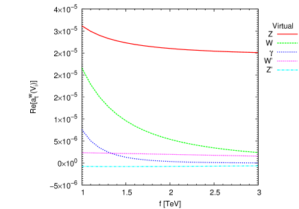
(a)

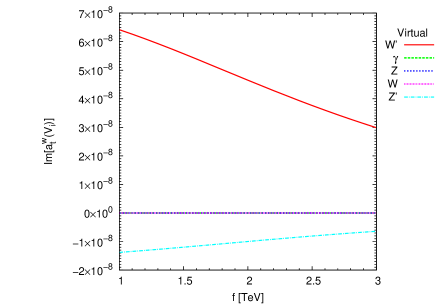
(b)

Figure 4: Individual vector contributions to $a^{W}_{t}$ in the BLHM for a fixed value of $F=4000\,\text{GeV}$. a) Re($a^{W}_{t}$). b) Im($a^{W}_{t}$).

The total contribution on the AWMDM of the top-quark involving scalar bosons, vector bosons, and exotic quarks in the loop is given in Fig. 5. In the range of analysis established for the $f$ scale, the total contribution on the AWMDM receives contributions coming mainly from two sectors: scalar and vector. Each sector arises from the sum of all scalar and vector contributions, respectively. In this manner, in Fig. 5 (a) we can appreciate the real contributions to $a^{W}_{t}$ and we find that the significant contribution to the total contribution comes from the scalar contribution, as both of which contribute in the order of magnitude of $10^{-4}$ to $10^{-5}$. On the other hand, the subdominant contribution is generated by the vectors: $\text{Re}[a^{W}_{t}(\text{vector})]\sim 10^{-5}$ for $f\in[1000,3000]$ GeV. Concerning Fig. 5 (b), the relevant contribution to the imaginary part of the AWMDM of the top arises from the scalar contribution, this contributes to the order of $10^{-5}$ to $10^{-6}$. The vector contribution is of the order of $10^{-8}$. The values of the total contribution to $a^{W}_{t}$ are listed in Table 1.

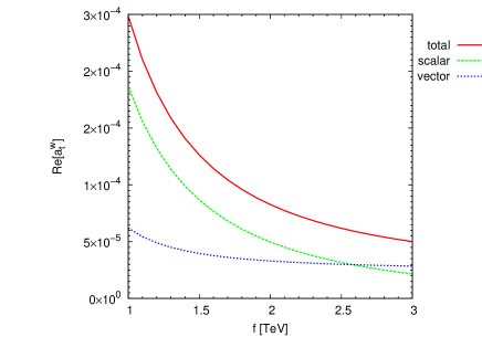
(a)

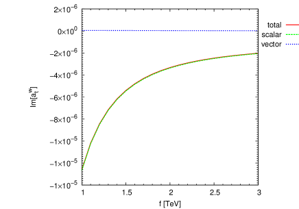
(b)

Figure 5: Scalar, vector and total contributions to $a^{W}_{t}$ in the BLHM for fixed values of $m_{A_{0}}=1000\,\text{GeV}$, $m_{\eta^{0}}=100\,\text{GeV}$ and $F=4000\,\text{GeV}$. a) Re($a^{W}_{t}$). b) Im($a^{W}_{t}$).

Since the masses of the states, $A_{0}$ and $\eta_{0}$ are input parameters of the BLHM, in order to measure the sensitivity of the AWMDM of the top-quark, we allow us to vary the masses of the mentioned states. For the pseudoscalar $A_{0}$ we have chosen the values of $m_{A_{0}}=1000,1500$ GeV, while for the neutral scalar $\eta^{0}$ we chose $m_{\eta^{0}}=100,500$ GeV. In this way, we generate the Figs. 6 and 7 that show the behavior of the real and imaginary part of $a^{W}_{t}$ when the energy scale $f$ varies from $1000$ GeV to $3000$ GeV, while fixing the other free parameters of the model. With the two fixed values of $m_{A_{0}}$, identical plots are generated as shown in Fig. 6 (a), this indicates that Re[$a^{W}_{t}$] is indifferent to the chosen values of the mass of the pseudoscalar $A_{0}$. Fig. 6 (b) shows plots with a very slight difference, since both contribute to the same order of magnitude. For the established values of $m_{\eta^{0}}$, in Fig. 7 (a) we observe that $|\text{Re}\,[a^{W}_{t}]|$ obtains more intense values when the mass of the $\eta^{0}$ scalar is small, specifically when $m_{\eta^{0}}=100$ GeV, $|\text{Re}\,[a^{W}_{t}]|\in[2.49\times 10^{-4},5.01\times 10^{-5}]$. The same pattern occurs in Fig. 7 (b), in this case $|\text{Im}\,[a^{W}_{t}]|\in[1.26\times 10^{-5},2.03\times 10^{-6}]$ for $m_{\eta^{0}}=100$ GeV. This result is to be expected since the contribution to AWMDM of the top-quark decouples as $m_{\eta^{0}}$ increases. For the different scenarios considered above, we provide the values of $a^{W}_{t}$ in Tables 1-3.

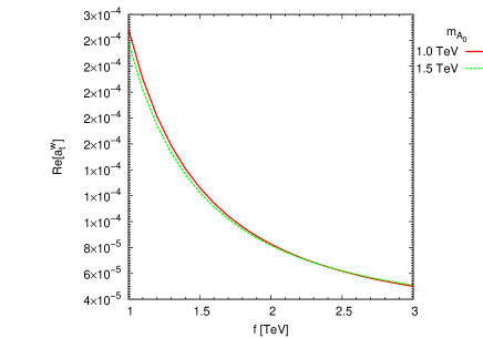
(a)

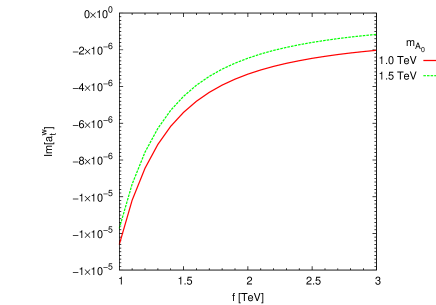
(b)

Figure 6: Total contribution to $a^{W}_{t}$ in the BLHM for different values of the mass of $A_{0}$ but fixed values of $m_{\eta^{0}}=100\,\text{GeV}$ and $F=4000\,\text{GeV}$. a) Re($a^{W}_{t}$). b) Im($a^{W}_{t}$).

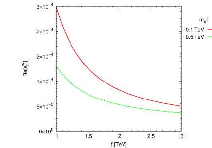
(a)

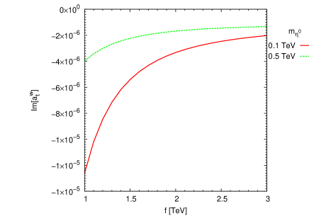
(b)

Figure 7: Total contribution to $a^{W}_{t}$ in the BLHM for different values of the mass of $\eta^{0}$ and fixed values of $m_{A_{0}}=1000\,\text{GeV}$ and $F=4000\,\text{GeV}$. a) Re($a^{W}_{t}$). b) Im($a^{W}_{t}$).

Another input parameter of the BLHM is $\tan\beta$, the values it acquires are restricted to the intervals generated according to Eq. (78). Therefore, if $m_{A_{0}}$ varies from 1000 GeV to 1500 GeV, $\tan\beta\in(1,10.45)$. For certain fixed values of $\tan\beta$, we obtain the behavior of $a^{W}_{t}$ as a function of the mass of the pseudoscalar $A_{0}$. In Fig. 8, we observe that $|\text{Re}\,[a^{W}_{t}]|$ obtains large values when $\tan\beta=3$ while $\tan\beta=6$ and $\tan\beta=10$ yield suppressed contributions to $a^{W}_{t}$. With respect to $|\text{Im}\,[a^{W}_{t}]|$, it also acquires high values when $\tan\beta=3$. According to Figs. 8 (a) and 8 (b) , it can be seen that for the different fixed values of $\tan\beta$, $|\text{Re}\,[a^{W}_{t}]|\sim 10^{-4}$ and $|\text{Im}\,[a^{W}_{t}]|\sim 10^{-5}$ are obtained.

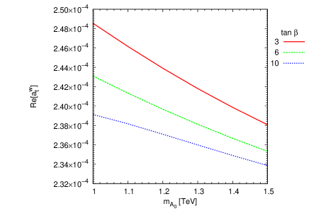
(a)

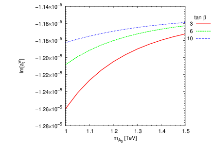
(b)

Figure 8: Total contribution to $a^{W}_{t}$ in the BLHM for different values of $\tan\beta$ and fixed values of $f=1000\,\text{GeV}$, $m_{\eta^{0}}=100\,\text{GeV}$ and $F=4000\,\text{GeV}$. a) Re($a^{W}_{t}$). b) Im($a^{W}_{t}$).

The two symmetry breaking energy scales are also free and important parameters of the BLHM, which we can vary. First, it can be seen from Fig. 9 (a) that $|\text{Re}\,[a^{W}_{t}]|$ does not essentially depend on $F$ parameter variations, while in Fig. 9 (b), $|\text{Im}\,[a^{W}_{t}]|$ does depend slightly on $F$. These plots show a variation of the $F$ parameter from $3000$ GeV to $6000$ GeV, for three distinct energy scales, i.e. $f=1,2,3$ TeV. In these figures, the main contributions to $|a^{W}_{t}|$ are generated for $f=1$ TeV, while secondary contributions arise for $f=2$ TeV. Second, Fig. 10 visualizes the behavior of $|\text{Re}\,[a^{W}_{t}]|$ and $|\text{Im}\,[a^{W}_{t}]|$ as a function of the $f$ scale. In this case, the graphs do depend on the variations of the parameter $f$. We have adopted the followings specific values for the parameter $F$, $F=4,5,6$ TeV so that the contribution to $|a^{W}_{t}]|$ is enhanced. However, there is not significant difference in the behavior of these plots. According to Eq. (96), the energy scale $f$ is also intimately related to the measure of the fine-tuning, and we observed that for $f=1$ TeV not only large contributions are generated for $|[a^{W}_{t}]|$, we also ensure the absence of fine-tuning.

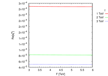
(a)

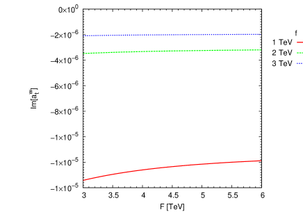
(b)

Figure 9: Total contribution to $a^{W}_{t}$ in the BLHM for different values of the energy scale $f$ with fixed values of $m_{A_{0}}=1000\,\text{GeV}$ and $m_{\eta^{0}}=100\,\text{GeV}$. a) Re($a^{W}_{t}$). b) Im($a^{W}_{t}$).

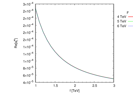
(a)

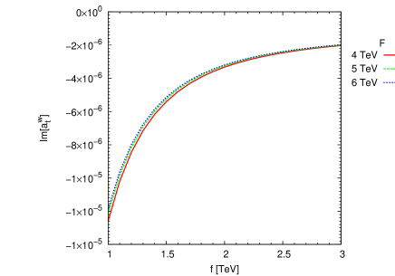
(b)

Figure 10: Total contribution to $a^{W}_{t}$ in the BLHM for different values of the energy scale $F$ with fixed values of $m_{A_{0}}=1000\,\text{GeV}$ and $m_{\eta^{0}}=100\,\text{GeV}$. a) Re($a^{W}_{t}$). b) Im($a^{W}_{t}$).

We have calculated the one-loop level contributions on the AWMDM of the top-quark in several scenarios. We found that the real and imaginary parts of $a^{W}_{t}$ is in the range $10^{-4}$ to $10^{-12}$ when the parameters $f$, $F$ and $m_{A_{0}}$ are varied in the corresponding intervals: $f=[1000,3000]$ GeV, $F=[3000,6000]$ GeV and $m_{A_{0}}=[1000,1500]$ GeV. The scalar sector provide the largest numerical contributions to $|\text{Re}\,[a^{W}_{t}]|$ and $|\text{Im}\,[a^{W}_{t}]|$. In general, $|\text{Im}\,[a^{W}_{t}]|$ is suppressed compared to $|\text{Re}\,[a^{W}_{t}]|$. In addition, we have found that our results are sensitive to changes in the value of $m_{\eta^{0}}$. The contribution to AWMDM from the top-quark decouples with large masses of the $\eta^{0}$ scalar, as shown in Fig. 7. Since our main goal in this work is to study the effect of the new particles generated in the BLHM framework, our results reported in this work on $a^{W}_{t}$ depend on the energy scales $f$ and $F$, which represent the scales of the new physics. In this scenario, we have found that the numerical values found for the AWMDM of the top-quark are comparable with the predictions of the SM or BSM. In the context of the SM, Bernabeu et al. Bernabeu:1995gs , they found that the numerical predictions for $a^{W}_{t}$ are on the order of $10^{-3}$. In Ref. Bernreuther:2005gq the one-loop level QCD contribution to the AWMDM of the top quark in the SM scenario has also been calculated, finding that $a^{W}_{t}=5.2\times 10^{-3}$ for renormalization scale $\mu=m_{t}=175$ GeV. Within the Minimal Supersymmetric Standard Model (MSSM), the contributions found for the AWMDM of the top-quark are on the order of magnitude of $10^{-4}$ Bartl:1997iq . In models with Two Higgs Doublets (2HDM), the induced effects of new scalars in the $t\bar{t}Z$ vertex loop were also investigated, obtaining $a^{W}_{t}\sim 10^{-3}$ Bernabeu:1995gs . Other studies performed in extended models that predict the existence of new $Z^{\prime}$ gauge boson, is obtained $a^{W}_{t}\in[10^{-6},10^{-10}]$ Vivian:2019zfa .

On the experimental side, the weak dipole moments of the top-quark have not yet been tested directly. There are promising project at colliders such as the LHC ATLAS:2016wgc ; Rontsch:2015una , the future ILC Behnke:2013xla ; Baer:2013cma ; Adolphsen:2013kya , the CLIC deBlas:2018mhx ; Robson:2018enq ; Roloff:2018dqu ; CLIC:2016zwp ; Abramowicz:2016zbo and the Future Circular Collider hadron-hadron (FCC-hh) Barletta:2014vea ; Koratzinos:2015fya that have as an important part of their physics program to investigate and constrain the dipole moments of the top-quark, in particular, the AWMDM. Currently, in the LHC experiment, the most hopeful avenue for studying the top-quark electroweak couplings is through the $pp\rightarrow\bar{t}tV$ ($V=Z,\gamma,H$) processes, which produces direct sensitivity without intrinsic dilution by QCD effects. In the FCC with proton-proton collisions, SM particles will also be produced in great abundance, and in this case, the study of the AWMDM can be carried out through the $pp\rightarrow\bar{t}tZ$ process. At a leptonic collider such as the ILC or CLIC, the focus of investigation will be via the $e^{+}e^{-}\rightarrow Z^{*}/\gamma\rightarrow\bar{t}t$ process which is extremely sensitive to top-quark electroweak couplings.

From the phenomenological point of view, for instance, through the production cross-section of $t\bar{t}ZZ$, limits on $a^{W}_{t}$ are estimated at $95\ \%$ C.L. corresponding to $3000$ fb^-1 of integrated luminosity at the LHC: $-0.1\leq a^{W}_{t}\leq 0.09$ Etesami:2017ufk . In this same integrated luminosity scenario, and through the $p^{Z}_{T}$ distribution in $\bar{t}tZ$ production, it is found that $-0.08\lesssim a^{W}_{t}\lesssim 0.08$ Rontsch:2015una . FCC-hh will provide collisions at a center-of-mass energy of 100 TeV, a factor 7 higher than the LHC. At this energy and with 10 000 fb^-1 of data, about $10^{8}$ $\bar{t}tZ$ events will be produced. At a rough estimate, the FCC-hh will provide improved limits to $a^{W}_{t}$ by a factor of 3 to 10 compared to the 3000 fb^-1 LHC Rontsch:2015una ; Barletta:2014vea ; Koratzinos:2015fya . Finally, at the ILC with $\sqrt{s}=500$ GeV and 500 fb^-1, the limits of $-0.02\lesssim a^{W}_{t}\lesssim 0.04$ at $95\ \%$ C.L. are expected to be reached. They are derived by exploiting the total cross-section of the top-quark pair production Rontsch:2015una . The ILC offers the possibility of extending the LHC top-quark program Baer:2013cma and is one of the most advanced proposals for an $e^{+}e^{-}$ collider. In the case of the ILC there is an improvement in the $a^{W}_{t}$ by a factor of three (through $\bar{t}tZ$ production) or four (through $\bar{t}tZZ$ production) compared to the LHC constraints. For these reasons, we believe that our results can be verified by the ILC in the future because it has the potential to reach the required level of sensitivity.

IV Conclusions

In this paper, we present a new comprehensive study on the sensitivity limits of the AWMDM of the top-quark in the context of the BLHM at the one-loop level. In our study, we have taken into account all contributions from the scalar sector, gauge sector, and heavy quarks. For which we deduced the allowed ranges of the masses of the new quarks, scalars, and vector bosons (see Eqs. (81) - (95)), as well as the corresponding Feynman rules of the BLHM expanded up to $\mathcal{O}(\frac{1}{f^{2}})$ (see Tables 4 - 17). These results are an original contribution.

The sensitivity on the AWMDM of the top-quark has been explored in the region of the parameter space allowed by the fine-tuning constraints, and measured by varying the main free parameters of the BLHM: $m_{A_{0}}$, $m_{\eta^{0}}$, $f$, $F$ and $\tan\beta$. Our results are summarized through a set of Figs. (2) - (10), Tables 1 - 3 (Sensitivity limits on the AWMDM at the BLHM) and Tables 4 - 17 (Feynman rules for the BLHM). We find that with the appropriated parameters of the BLHM it is possible to put limits on the AWMDM of the top-quark with a sensitivity of the order of $a^{W}_{t}=2.49\times 10^{-4}-1.26\times 10^{-5}i$, $1.26\times 10^{-4}-5.41\times 10^{-6}i$, where the main contribution comes from the scalars $h_{0}$ and $H_{0}$. The sensitivity limits on $a^{W}_{t}$ obtained in the context of the BLHM (see Tables 1 - 3) are competitive concerning for to the reported in Refs. Bernabeu:1995gs ; Bernreuther:2005gq ; Bartl:1997iq ; Vivian:2019zfa , and in some cases compare favorably. We should remark that our results found for $a^{W}_{t}$ fall within the phenomenological bounds provided by colliders such as LHC, FCC-hh and ILC Etesami:2017ufk ; Rontsch:2015una ; Barletta:2014vea ; Koratzinos:2015fya . Present, there are no precision experimental measurements on the AWMDM of the top-quark. However, future proposed experiments are expected to reach sensitivity to predicted values for observables in the BLHM. In addition, as this topic is worthwhile yet underexplored, theoretical, experimental and phenomenological interest is of great importance in order to motivate experimental collaborations to measure this very intriguing sector of the SM, which could give evidence of new physics BSM.

Table 1: Expected sensitivity limits on the $a^{W}_{t}$ in the context of the BLHM with $\sqrt{q^{2}}=500\ \text{GeV}$,  $\text{m}_{A_{0}}=1000\ \text{GeV}$, $\text{m}_{\eta_{0}}=100\ \text{GeV}$, $F=4000\ \text{GeV}$ and $f=1,1.5,2,2.5,3\ \text{TeV}$ are represented. All new contributions are considered, scalar bosons, vector bosons and heavy quarks.

$\sqrt{q^{2}}=500\ \text{GeV}$, $\text{m}_{A_{0}}=1000\ \text{GeV}$, $\text{m}_{\eta_{0}}=\bf{100}\ \text{GeV}$, $F=4000\ \text{GeV}$
$f\ [\text{TeV}]$	$(a^{W}_{t})^{\rm Total}$
$1_{\cdot}0$	$2_{\cdot}49\times 10^{-4}-1_{\cdot}26\times 10^{-5}\ i$
$1_{\cdot}5$	$1_{\cdot}26\times 10^{-4}-5_{\cdot}41\times 10^{-6}\ i$
$2_{\cdot}0$	$8_{\cdot}26\times 10^{-5}-3_{\cdot}33\times 10^{-6}\ i$
$2_{\cdot}5$	$6_{\cdot}18\times 10^{-5}-2_{\cdot}47\times 10^{-6}\ i$
$3_{\cdot}0$	$5_{\cdot}01\times 10^{-5}-2_{\cdot}03\times 10^{-6}\ i$

Table 2: Expected sensitivity limits on the $a^{W}_{t}$ in the context of the BLHM with $\sqrt{q^{2}}=500\ \text{GeV}$,  $\text{m}_{A_{0}}=1000\ \text{GeV}$, $\text{m}_{\eta_{0}}=500\ \text{GeV}$, $F=4000\ \text{GeV}$ and $f=1,1.5,2,2.5,3\ \text{TeV}$ are represented. All new contributions are considered, scalar bosons, vector bosons and heavy quarks.

$\sqrt{q^{2}}=500\ \text{GeV}$, $\text{m}_{A_{0}}=1000\ \text{GeV}$, $\text{m}_{\eta_{0}}=\bf{500}\ \text{GeV}$, $\ F=4000\ \text{GeV}$
$f\ [\text{TeV}]$	$(a^{W}_{t})^{\rm Total}$
$1_{\cdot}0$	$1_{\cdot}31\times 10^{-4}-3_{\cdot}99\times 10^{-6}\ i$
$1_{\cdot}5$	$7_{\cdot}40\times 10^{-5}-2_{\cdot}23\times 10^{-6}\ i$
$2_{\cdot}0$	$5_{\cdot}32\times 10^{-5}-1_{\cdot}68\times 10^{-6}\ i$
$2_{\cdot}5$	$4_{\cdot}29\times 10^{-5}-1_{\cdot}45\times 10^{-6}\ i$
$3_{\cdot}0$	$3_{\cdot}69\times 10^{-5}-1_{\cdot}33\times 10^{-6}\ i$

Table 3: Expected sensitivity limits on the $a^{W}_{t}$ in the context of the BLHM with $\sqrt{q^{2}}=500\ \text{GeV}$,  $\text{m}_{A_{0}}=1500\ \text{GeV}$, $\text{m}_{\eta_{0}}=100\ \text{GeV}$, $F=4000\ \text{GeV}$ and $f=1,1.5,2,2.5,3\ \text{TeV}$ are represented. All new contributions are considered, scalar bosons, vector bosons and heavy quarks.

$\sqrt{q^{2}}=500\ \text{GeV}$, $\text{m}_{A_{0}}=\bf{1500}\ \text{GeV}$, $\text{m}_{\eta_{0}}=100\ \text{GeV}$, $\ F=4000\ \text{GeV}$
$f\ [\text{TeV}]$	$(a^{W}_{t})^{\rm Total}$
$1_{\cdot}0$	$2_{\cdot}38\times 10^{-4}-1_{\cdot}17\times 10^{-5}\ i$
$1_{\cdot}5$	$1_{\cdot}23\times 10^{-4}-4_{\cdot}53\times 10^{-6}\ i$
$2_{\cdot}0$	$8_{\cdot}17\times 10^{-5}-2_{\cdot}46\times 10^{-6}\ i$
$2_{\cdot}5$	$6_{\cdot}20\times 10^{-5}-1_{\cdot}60\times 10^{-6}\ i$
$3_{\cdot}0$	$5_{\cdot}09\times 10^{-5}-1_{\cdot}16\times 10^{-6}\ i$

Acknowledgements

E. C. A. appreciates the post-doctoral stay. A. G. R. thank SNI and PROFEXCE (México).

Appendix A Feynman rules for the BLHM

In this appendix we present the complete set of Feynman rules for the BLHM involved in our calculation for the AWMDM of the top-quark.

It is convenient to define the following useful notation:

$$c_{\beta} = \cos\beta,$$ (98)

$$s_{\beta} = \sin\beta,$$ (99)

$$s_{\alpha} = \sin\alpha,$$ (100)

$$c_{\alpha} = \cos\alpha.$$ (101)

$$u_{i} = u,c.$$ (102)

$$d_{i} = d,s.$$ (103)

$$e_{i} = e,\mu,\tau.$$ (104)

$$\nu_{i} = \nu_{e},\nu_{\mu},\nu_{\tau}.$$ (105)

$$y_{f} = \frac{m_{f}}{v\sin\beta}\left(1-\frac{v^{2}}{3f^{2}}\right)^{-1/2}.$$ (106)

Table 4: Feynman rules for the BLHM involving the pseudoscalar $A_{0}$.

Vertex	Feynman rules
$A_{0}t\bar{t}$	$-\frac{3ic_{\beta}(P_{L}-P_{R})y_{1}y_{2}y_{3}}{\sqrt{y_{1}^{2}+y_{2}^{2}}\sqrt{y_{1}^{2}+y_{3}^{2}}}+\frac{2ic_{\beta}(P_{L}-P_{R})s_{\beta}vy_{2}\left(y_{3}^{2}-2y_{1}^{2}\right)y_{3}}{f\sqrt{y_{1}^{2}+y_{2}^{2}}\left(y_{1}^{2}+y_{3}^{2}\right)}\hfill\break+\frac{3ic_{\beta}(P_{L}-P_{R})s_{\beta}^{2}v^{2}y_{1}y_{2}\left(4y_{1}^{6}+4\left(2y_{2}^{2}+y_{3}^{2}\right)y_{1}^{4}+\left(4y_{2}^{4}+8y_{3}^{2}y_{2}^{2}-2\sqrt{y_{1}^{2}+y_{3}^{2}}\right)y_{1}^{2}+y_{2}^{2}\left(4y_{2}^{2}y_{3}^{2}+\sqrt{y_{1}^{2}+y_{3}^{2}}\right)\right)y_{3}^{3}}{2f^{2}\left(y_{1}^{2}+y_{2}^{2}\right)^{5/2}\left(y_{1}^{2}+y_{3}^{2}\right)^{5/2}}$
$A_{0}T\bar{T}$	$\frac{ic_{\beta}(P_{L}-P_{R})s_{\beta}vy_{1}^{2}\left(\left(y_{2}^{2}+2y_{3}^{2}\right)y_{1}^{4}+\left(8y_{2}^{2}y_{3}^{2}-2y_{3}^{4}\right)y_{1}^{2}-y_{2}^{2}\left(y_{2}^{4}+3y_{3}^{2}y_{2}^{2}-7y_{3}^{4}\right)\right)}{f\left(y_{1}^{2}+y_{2}^{2}\right)^{3/2}\left(y_{2}^{2}-y_{3}^{2}\right)\left(y_{1}^{2}+y_{3}^{2}\right)}$
$A_{0}T_{5}\bar{T}_{5}$	$\frac{9ic_{\beta}(P_{L}-P_{R})s_{\beta}vy_{1}^{2}y_{2}^{2}y_{3}^{2}}{f\left(y_{1}^{2}+y_{3}^{2}\right)^{3/2}\left(y_{3}^{2}-y_{2}^{2}\right)}$
$A_{0}T_{6}\bar{T}_{6}$	$\frac{ic_{\beta}(P_{R}-P_{L})s_{\beta}vy_{1}}{f}$
$A_{0}T^{2/3}\bar{T}^{2/3}$	$\frac{ic_{\beta}(P_{L}-P_{R})s_{\beta}vy_{1}\left(3y_{1}^{2}-5y_{3}^{2}\right)}{f\left(y_{1}^{2}+y_{3}^{2}\right)}$
$A_{0}b\bar{b}$	$ic_{\beta}(P_{L}-P_{R})y_{b}$
$A_{0}t\bar{T}$	$\frac{ic_{\beta}P_{R}\left(2y_{1}^{2}-y_{2}^{2}\right)y_{3}}{\sqrt{y_{1}^{2}+y_{2}^{2}}\sqrt{y_{1}^{2}+y_{3}^{2}}}+\frac{ic_{\beta}s_{\beta}vy_{1}\left(P_{L}y_{2}\left(2y_{1}^{4}+\left(2y_{2}^{2}+5y_{3}^{2}\right)y_{1}^{2}-4y_{2}^{2}y_{3}^{2}\right)-2P_{R}y_{3}\left(-y_{1}^{4}+y_{3}^{2}y_{1}^{2}+y_{2}^{4}+y_{2}^{2}y_{3}^{2}\right)\right)}{f\left(y_{1}^{2}+y_{2}^{2}\right)^{3/2}\left(y_{1}^{2}+y_{3}^{2}\right)}\hfill\break+\frac{3ic_{\beta}P_{R}s_{\beta}^{2}v^{2}y_{1}^{2}\left(4y_{1}^{6}+4\left(2y_{2}^{2}+y_{3}^{2}\right)y_{1}^{4}+\left(4y_{2}^{4}+8y_{3}^{2}y_{2}^{2}-2\sqrt{y_{1}^{2}+y_{3}^{2}}\right)y_{1}^{2}+y_{2}^{2}\left(4y_{2}^{2}y_{3}^{2}+\sqrt{y_{1}^{2}+y_{3}^{2}}\right)\right)y_{3}^{3}}{2f^{2}\left(y_{1}^{2}+y_{2}^{2}\right)^{5/2}\left(y_{2}^{2}-y_{3}^{2}\right)\left(y_{1}^{2}+y_{3}^{2}\right)^{3/2}}$
$A_{0}t\bar{T}_{5}$	$-\frac{ic_{\beta}P_{L}\left(2y_{1}^{2}-y_{3}^{2}\right)y_{2}}{\sqrt{y_{1}^{2}+y_{2}^{2}}\sqrt{y_{1}^{2}+y_{3}^{2}}}+\frac{ic_{\beta}P_{R}s_{\beta}vy_{1}y_{3}}{2f\left(y_{1}^{2}+y_{2}^{2}\right)^{2}\left(y_{1}^{2}+y_{3}^{2}\right)^{3/2}\left(y_{3}^{2}-y_{2}^{2}\right)}\hfill\break\times\bigg{(}4\left(2y_{2}^{2}+y_{3}^{2}\right)y_{1}^{6}+2\left(8y_{2}^{4}-y_{3}^{2}y_{2}^{2}+2y_{3}^{4}\right)y_{1}^{4}+2\left(y_{2}^{2}-y_{3}^{2}\right)\left(4y_{2}^{4}-4y_{3}^{2}y_{2}^{2}+\sqrt{y_{1}^{2}+y_{3}^{2}}\right)y_{1}^{2}\hfill\break-10y_{2}^{6}y_{3}^{2}-y_{2}^{4}\left(\sqrt{y_{1}^{2}+y_{3}^{2}}-4y_{3}^{4}\right)+y_{2}^{2}y_{3}^{2}\sqrt{y_{1}^{2}+y_{3}^{2}}\bigg{)}\hfill\break+\frac{3ic_{\beta}s_{\beta}^{2}v^{2}y_{1}^{2}y_{3}\left(3P_{L}y_{2}y_{3}\left(y_{1}^{2}+y_{3}^{2}\right)-2P_{R}\sqrt{y_{1}^{2}+y_{2}^{2}}\left(y_{1}^{2}-2y_{3}^{2}\right)\sqrt{y_{1}^{2}+y_{3}^{2}}\right)y_{2}^{2}}{f^{2}\sqrt{y_{1}^{2}+y_{2}^{2}}\left(y_{2}^{2}-y_{3}^{2}\right)\left(y_{1}^{2}+y_{3}^{2}\right)^{5/2}}$
$A_{0}t\bar{T}_{6}$	$\frac{2iP_{L}s_{\beta}y_{1}y_{2}}{\sqrt{y_{1}^{2}+y_{2}^{2}}}-\frac{ivP_{R}y_{1}y_{3}}{2f}\hfill\break\times\frac{\left(4y_{1}^{6}+4\left(2y_{2}^{2}+y_{3}^{2}\right)y_{1}^{4}+\left(4y_{2}^{4}+8y_{3}^{2}y_{2}^{2}-2\sqrt{y_{1}^{2}+y_{3}^{2}}\right)y_{1}^{2}+y_{2}^{2}\left(4y_{2}^{2}y_{3}^{2}+\sqrt{y_{1}^{2}+y_{3}^{2}}\right)\right)s_{\beta}^{2}+8c_{\beta}^{2}\left(y_{1}^{2}+y_{2}^{2}\right)^{2}\left(y_{1}^{2}+y_{3}^{2}\right)}{\left(y_{1}^{2}+y_{2}^{2}\right)^{2}\left(y_{1}^{2}+y_{3}^{2}\right)^{3/2}}\hfill\break+\frac{ic_{\beta}^{2}s_{\beta}y_{3}\left(3P_{L}y_{1}y_{2}y_{3}+4P_{R}\sqrt{y_{1}^{2}+y_{2}^{2}}\left(y_{3}^{2}-y_{1}^{2}\right)\right)}{f^{2}\sqrt{y_{1}^{2}+y_{2}^{2}}\left(y_{1}^{2}+y_{3}^{2}\right)}$
$A_{0}t\bar{T}^{2/3}$	$-\frac{2ic_{\beta}P_{R}y_{1}y_{3}}{\sqrt{y_{1}^{2}+y_{3}^{2}}}-\frac{ic_{\beta}s_{\beta}\left(P_{L}y_{1}y_{2}\left(4y_{1}^{2}-11y_{3}^{2}\right)+2P_{R}\sqrt{y_{1}^{2}+y_{2}^{2}}y_{3}\left(y_{1}^{2}-y_{3}^{2}\right)\right)v}{f\sqrt{y_{1}^{2}+y_{2}^{2}}\left(y_{1}^{2}+y_{3}^{2}\right)}\hfill\break-\frac{ic_{\beta}P_{R}s_{\beta}^{2}y_{1}y_{3}\left(4y_{1}^{6}+4\left(2y_{2}^{2}+y_{3}^{2}\right)y_{1}^{4}+\left(4y_{2}^{4}+8y_{3}^{2}y_{2}^{2}-2\sqrt{y_{1}^{2}+y_{3}^{2}}\right)y_{1}^{2}+y_{2}^{2}\left(4y_{2}^{2}y_{3}^{2}+\sqrt{y_{1}^{2}+y_{3}^{2}}\right)\right)v^{2}}{2f^{2}\left(y_{1}^{2}+y_{2}^{2}\right)^{2}\left(y_{1}^{2}+y_{3}^{2}\right)^{3/2}}$

Table 5: Feynman rules for the BLHM involving the scalar $h_{0}$.

Vertex	Feynman rules
$h_{0}T\bar{T}$	$\frac{c_{\alpha}s_{\beta}vy_{1}^{2}\left(\left(y_{2}^{2}+2y_{3}^{2}\right)y_{1}^{4}+\left(8y_{2}^{2}y_{3}^{2}-2y_{3}^{4}\right)y_{1}^{2}-y_{2}^{2}\left(y_{2}^{4}+3y_{3}^{2}y_{2}^{2}-7y_{3}^{4}\right)\right)}{f\left(y_{1}^{2}+y_{2}^{2}\right)^{3/2}\left(y_{2}^{2}-y_{3}^{2}\right)\left(y_{1}^{2}+y_{3}^{2}\right)}$
$h_{0}T_{5}\bar{T}_{5}$	$\frac{9c_{\alpha}s_{\beta}vy_{1}^{2}y_{2}^{2}y_{3}^{2}}{f\left(y_{1}^{2}+y_{3}^{2}\right)^{3/2}\left(y_{3}^{2}-y_{2}^{2}\right)}$
$h_{0}T_{6}\bar{T}_{6}$	$-\frac{c_{\beta}s_{\alpha}vy_{1}}{f}$
$h_{0}T^{2/3}\bar{T}^{2/3}$	$-\frac{vy_{1}\left(4c_{\alpha}s_{\beta}\left(y_{1}^{2}-y_{3}^{2}\right)+\text{c$\beta$}s_{\alpha}\left(y_{1}^{2}+y_{3}^{2}\right)\right)}{f\left(y_{1}^{2}+y_{3}^{2}\right)}$
$h_{0}t\bar{T}$	$\frac{c_{\alpha}P_{R}\left(y_{2}^{2}-2y_{1}^{2}\right)y_{3}}{\sqrt{y_{1}^{2}+y_{2}^{2}}\sqrt{y_{1}^{2}+y_{3}^{2}}}+\frac{c_{\alpha}s_{\beta}y_{1}\left(2P_{R}y_{3}\left(-y_{1}^{4}+y_{3}^{2}y_{1}^{2}+y_{2}^{4}+y_{2}^{2}y_{3}^{2}\right)+P_{L}y_{2}\left(2y_{1}^{4}+\left(2y_{2}^{2}+5y_{3}^{2}\right)y_{1}^{2}-4y_{2}^{2}y_{3}^{2}\right)\right)v}{f\left(y_{1}^{2}+y_{2}^{2}\right)^{3/2}\left(y_{1}^{2}+y_{3}^{2}\right)}$
$h_{0}t\bar{T}_{5}$	$\frac{c_{\alpha}P_{L}y_{2}\left(y_{3}^{2}-2y_{1}^{2}\right)}{\sqrt{y_{1}^{2}+y_{2}^{2}}\sqrt{y_{1}^{2}+y_{3}^{2}}}-\frac{c_{\alpha}P_{R}vs_{\beta}y_{1}y_{3}}{2f\left(y_{1}^{2}+y_{2}^{2}\right)^{2}\left(y_{1}^{2}+y_{3}^{2}\right)^{3/2}\left(y_{3}^{2}-y_{2}^{2}\right)}\bigg{(}4\left(2y_{2}^{2}+y_{3}^{2}\right)y_{1}^{6}+2\left(8y_{2}^{4}-y_{3}^{2}y_{2}^{2}+2y_{3}^{4}\right)y_{1}^{4}\hfill\break+2\left(y_{2}^{2}-y_{3}^{2}\right)\left(4y_{2}^{4}-4y_{3}^{2}y_{2}^{2}+\sqrt{y_{1}^{2}+y_{3}^{2}}\right)y_{1}^{2}-10y_{2}^{6}y_{3}^{2}-y_{2}^{4}\left(\sqrt{y_{1}^{2}+y_{3}^{2}}-4y_{3}^{4}\right)\hfill\break+y_{2}^{2}y_{3}^{2}\sqrt{y_{1}^{2}+y_{3}^{2}}\bigg{)}$
$h_{0}t\bar{T}_{6}$	$-\frac{2P_{L}s_{\alpha}y_{1}y_{2}}{\sqrt{y_{1}^{2}+y_{2}^{2}}}+\frac{vP_{R}y_{1}y_{3}}{2f\left(y_{1}^{2}+y_{3}^{2}\right)^{3/2}}\bigg{(}8c_{\alpha}c_{\beta}\left(y_{1}^{2}+y_{3}^{2}\right)\hfill\break+\frac{s_{\alpha}s_{\beta}\left(4y_{1}^{6}+4\left(2y_{2}^{2}+y_{3}^{2}\right)y_{1}^{4}+2\left(2y_{2}^{4}+4y_{3}^{2}y_{2}^{2}+\sqrt{y_{1}^{2}+y_{3}^{2}}\right)y_{1}^{2}+4y_{2}^{4}y_{3}^{2}-y_{2}^{2}\sqrt{y_{1}^{2}+y_{3}^{2}}\right)}{\left(y_{1}^{2}+y_{2}^{2}\right)^{2}}\bigg{)}-\frac{v^{2}}{3f^{2}\sqrt{y_{1}^{2}+y_{2}^{2}}\left(y_{1}^{2}+y_{3}^{2}\right)}\times\hfill\break\bigg{(}12P_{L}s_{\alpha}y_{1}y_{2}\left(y_{1}^{2}+y_{3}^{2}\right)c_{\beta}^{2}+2c_{\alpha}s_{\beta}\left(P_{L}y_{1}y_{2}\left(4y_{1}^{2}-5y_{3}^{2}\right)-3P_{R}\sqrt{y_{1}^{2}+y_{2}^{2}}y_{3}\left(y_{1}^{2}-3y_{3}^{2}\right)\right)c_{\beta}\hfill\break+s_{\alpha}s_{\beta}^{2}\left(P_{L}y_{1}y_{2}\left(4y_{1}^{2}-5y_{3}^{2}\right)+6P_{R}\sqrt{y_{1}^{2}+y_{2}^{2}}y_{3}\left(y_{1}^{2}+y_{3}^{2}\right)\right)\bigg{)}$
$h_{0}t\bar{T}^{2/3}$	$-\frac{2c_{\alpha}P_{R}y_{1}y_{3}}{\sqrt{y_{1}^{2}+y_{3}^{2}}}+\frac{\left(2c_{\beta}P_{L}s_{\alpha}y_{1}y_{2}\left(y_{1}^{2}+y_{3}^{2}\right)+c_{\alpha}s_{\beta}\left(2P_{R}\sqrt{y_{1}^{2}+y_{2}^{2}}y_{3}\left(y_{3}^{2}-y_{1}^{2}\right)+P_{L}\left(7y_{1}y_{2}y_{3}^{2}-2y_{1}^{3}y_{2}\right)\right)\right)v}{f\sqrt{y_{1}^{2}+y_{2}^{2}}\left(y_{1}^{2}+y_{3}^{2}\right)}\hfill\break-\frac{P_{R}y_{1}y_{3}v^{2}}{6f^{2}\left(y_{1}^{2}+y_{2}^{2}\right)^{2}\left(y_{1}^{2}+y_{3}^{2}\right)^{3/2}}\bigg{(}6c_{\alpha}\hfill\break\times\left(2y_{1}^{6}+2\left(2y_{2}^{2}+y_{3}^{2}\right)y_{1}^{4}+2\left(y_{2}^{4}+2y_{3}^{2}y_{2}^{2}+\sqrt{y_{1}^{2}+y_{3}^{2}}\right)y_{1}^{2}+2y_{2}^{4}y_{3}^{2}-y_{2}^{2}\sqrt{y_{1}^{2}+y_{3}^{2}}\right)s_{\beta}^{2}+c_{\beta}s_{\alpha}\Big{(}4y_{1}^{6}+4\left(2y_{2}^{2}+y_{3}^{2}\right)y_{1}^{4}+\left(4y_{2}^{4}+8y_{3}^{2}y_{2}^{2}+6\sqrt{y_{1}^{2}+y_{3}^{2}}\right)y_{1}^{2}+4y_{2}^{4}y_{3}^{2}\hfill\break-3y_{2}^{2}\sqrt{y_{1}^{2}+y_{3}^{2}}\Big{)}s_{\beta}-4c_{\alpha}c_{\beta}^{2}\left(y_{1}^{2}+y_{2}^{2}\right)^{2}\left(y_{1}^{2}+y_{3}^{2}\right)\bigg{)}$

Table 6: Feynman rules for the BLHM involving the scalar $H_{0}$.

Vertex	Feynman rules
$H_{0}t\bar{t}$	$\frac{3s_{\alpha}y_{1}y_{2}y_{3}}{\sqrt{y_{1}^{2}+y_{2}^{2}}\sqrt{y_{1}^{2}+y_{3}^{2}}}-\frac{2s_{\alpha}s_{\beta}y_{2}y_{3}\left(y_{3}^{2}-2y_{1}^{2}\right)v}{f\sqrt{y_{1}^{2}+y_{2}^{2}}\left(y_{1}^{2}+y_{3}^{2}\right)}-\frac{y_{1}y_{2}y_{3}v^{2}}{2f^{2}\left(y_{1}^{2}+y_{2}^{2}\right)^{5/2}\left(y_{1}^{2}+y_{3}^{2}\right)^{5/2}}\bigg{(}s_{\alpha}\Big{(}14y_{1}^{8}+4\left(7y_{2}^{2}+4y_{3}^{2}\right)y_{1}^{6}\hfill\break+2\left(7y_{2}^{4}+16y_{3}^{2}y_{2}^{2}+y_{3}^{4}+2\sqrt{y_{1}^{2}+y_{3}^{2}}\right)y_{1}^{4}-2\big{(}-8y_{3}^{2}y_{2}^{4}+\left(\sqrt{y_{1}^{2}+y_{3}^{2}}-2y_{3}^{4}\right)y_{2}^{2}\hfill\break+y_{3}^{2}\sqrt{y_{1}^{2}+y_{3}^{2}}\big{)}y_{1}^{2}+y_{2}^{2}y_{3}^{2}\left(2y_{2}^{2}y_{3}^{2}+\sqrt{y_{1}^{2}+y_{3}^{2}}\right)\Big{)}s_{\beta}^{2}-2c_{\alpha}c_{\beta}\left(y_{1}^{2}+y_{3}^{2}\right)\hfill\break\times\left(6y_{1}^{6}+6\left(2y_{2}^{2}+y_{3}^{2}\right)y_{1}^{4}+2\left(3y_{2}^{4}+6y_{3}^{2}y_{2}^{2}+\sqrt{y_{1}^{2}+y_{3}^{2}}\right)y_{1}^{2}+6y_{2}^{4}y_{3}^{2}-y_{2}^{2}\sqrt{y_{1}^{2}+y_{3}^{2}}\right)s_{\beta}\hfill\break+2c_{\beta}^{2}s_{\alpha}\left(y_{1}^{2}+y_{2}^{2}\right)^{2}\left(y_{1}^{2}+y_{3}^{2}\right)^{2}\bigg{)}$
$H_{0}T\bar{T}$	$-\frac{s_{\alpha}s_{\beta}vy_{1}^{2}\left(\left(y_{2}^{2}+2y_{3}^{2}\right)y_{1}^{4}+\left(8y_{2}^{2}y_{3}^{2}-2y_{3}^{4}\right)y_{1}^{2}-y_{2}^{2}\left(y_{2}^{4}+3y_{3}^{2}y_{2}^{2}-7y_{3}^{4}\right)\right)}{f\left(y_{1}^{2}+y_{2}^{2}\right)^{3/2}\left(y_{2}^{2}-y_{3}^{2}\right)\left(y_{1}^{2}+y_{3}^{2}\right)}$
$H_{0}T_{5}\bar{T}_{5}$	$-\frac{9s_{\alpha}s_{\beta}vy_{1}^{2}y_{2}^{2}y_{3}^{2}}{f\left(y_{1}^{2}+y_{3}^{2}\right)^{3/2}\left(y_{3}^{2}-y_{2}^{2}\right)}$
$H_{0}T_{6}\bar{T}_{6}$	$-\frac{c_{\alpha}c_{\beta}vy_{1}}{f}$
$H_{0}T^{2/3}\bar{T}^{2/3}$	$-\frac{vy_{1}\left(4s_{\alpha}s_{\beta}\left(y_{3}^{2}-y_{1}^{2}\right)+c_{\alpha}c_{\beta}\left(y_{1}^{2}+y_{3}^{2}\right)\right)}{f\left(y_{1}^{2}+y_{3}^{2}\right)}$
$H_{0}b\bar{b}$	$s_{\alpha}y_{b}-\frac{\left(s_{\alpha}c_{\beta}^{2}-2c_{\alpha}s_{\beta}c_{\beta}+3s_{\alpha}s_{\beta}^{2}\right)v^{2}y_{b}}{3f^{2}}$
$H_{0}t\bar{T}$	$\frac{P_{R}s_{\alpha}\left(2y_{1}^{2}-y_{2}^{2}\right)y_{3}}{\sqrt{y_{1}^{2}+y_{2}^{2}}\sqrt{y_{1}^{2}+y_{3}^{2}}}-\frac{s_{\alpha}s_{\beta}y_{1}\left(2P_{R}y_{3}\left(-y_{1}^{4}+y_{3}^{2}y_{1}^{2}+y_{2}^{4}+y_{2}^{2}y_{3}^{2}\right)+P_{L}y_{2}\left(2y_{1}^{4}+\left(2y_{2}^{2}+5y_{3}^{2}\right)y_{1}^{2}-4y_{2}^{2}y_{3}^{2}\right)\right)v}{f\left(y_{1}^{2}+y_{2}^{2}\right)^{3/2}\left(y_{1}^{2}+y_{3}^{2}\right)}\hfill\break-\frac{P_{R}y_{3}v^{2}}{6f^{2}\left(y_{1}^{2}+y_{2}^{2}\right)^{5/2}\left(y_{2}^{2}-y_{3}^{2}\right)\left(y_{1}^{2}+y_{3}^{2}\right)^{3/2}}\bigg{(}3s_{\alpha}\Big{(}4\left(2y_{2}^{2}+y_{3}^{2}\right)y_{1}^{8}+2\left(5y_{2}^{4}+11y_{3}^{2}y_{2}^{2}+2y_{3}^{4}\right)y_{1}^{6}\hfill\break+2\left(-2y_{2}^{6}+13y_{3}^{2}y_{2}^{4}+\left(7y_{3}^{4}+\sqrt{y_{1}^{2}+y_{3}^{2}}\right)y_{2}^{2}+2y_{3}^{2}\sqrt{y_{1}^{2}+y_{3}^{2}}\right)y_{1}^{4}\hfill\break+y_{2}^{4}\left(-6y_{2}^{4}+2y_{3}^{2}y_{2}^{2}+16y_{3}^{4}-3\sqrt{y_{1}^{2}+y_{3}^{2}}\right)y_{1}^{2}-y_{2}^{4}\left(y_{3}^{2}-y_{2}^{2}\Big{)}\left(\sqrt{y_{1}^{2}+y_{3}^{2}}-6y_{2}^{2}y_{3}^{2}\right)\right)s_{\beta}^{2}+c_{\alpha}c_{\beta}\left(y_{3}^{2}-y_{2}^{2}\right)\bigg{(}20y_{1}^{8}+4\left(6y_{2}^{2}+5y_{3}^{2}\right)y_{1}^{6}+6\left(-2y_{2}^{4}+4y_{3}^{2}y_{2}^{2}+\sqrt{y_{1}^{2}+y_{3}^{2}}\right)y_{1}^{4}\hfill\break-\left(16y_{2}^{6}+12y_{3}^{2}y_{2}^{4}+9\sqrt{y_{1}^{2}+y_{3}^{2}}y_{2}^{2}\right)y_{1}^{2}-16y_{2}^{6}y_{3}^{2}+3y_{2}^{4}\sqrt{y_{1}^{2}+y_{3}^{2}}\bigg{)}s_{\beta}\hfill\break+2c_{\beta}^{2}s_{\alpha}\left(2y_{1}^{2}-y_{2}^{2}\right)\left(y_{1}^{2}+y_{2}^{2}\right)^{2}\left(y_{2}^{2}-y_{3}^{2}\right)\left(y_{1}^{2}+y_{3}^{2}\right)\bigg{)}$
$H_{0}t\bar{T}_{5}$	$\frac{P_{L}s_{\alpha}y_{2}\left(2y_{1}^{2}-y_{3}^{2}\right)}{\sqrt{y_{1}^{2}+y_{2}^{2}}\sqrt{y_{1}^{2}+y_{3}^{2}}}+\frac{P_{R}vs_{\alpha}s_{\beta}y_{1}y_{3}}{2f\left(y_{1}^{2}+y_{2}^{2}\right)^{2}\left(y_{1}^{2}+y_{3}^{2}\right)^{3/2}\left(y_{3}^{2}-y_{2}^{2}\right)}\hfill\break\times\bigg{(}4\left(2y_{2}^{2}+y_{3}^{2}\right)y_{1}^{6}+2\left(8y_{2}^{4}-y_{3}^{2}y_{2}^{2}+2y_{3}^{4}\right)y_{1}^{4}+2\left(y_{2}^{2}-y_{3}^{2}\right)\left(4y_{2}^{4}-4y_{3}^{2}y_{2}^{2}+\sqrt{y_{1}^{2}+y_{3}^{2}}\right)y_{1}^{2}-10y_{2}^{6}y_{3}^{2}-y_{2}^{4}\left(\sqrt{y_{1}^{2}+y_{3}^{2}}-4y_{3}^{4}\right)+y_{2}^{2}y_{3}^{2}\sqrt{y_{1}^{2}+y_{3}^{2}}\bigg{)}+\frac{v^{2}}{3f^{2}\sqrt{y_{1}^{2}+y_{2}^{2}}\left(y_{2}^{2}-y_{3}^{2}\right)\left(y_{1}^{2}+y_{3}^{2}\right)^{5/2}}\hfill\break\times\bigg{(}3s_{\alpha}y_{3}\Big{(}2P_{R}\sqrt{y_{1}^{2}+y_{2}^{2}}\sqrt{y_{1}^{2}+y_{3}^{2}}\left(-4y_{3}^{4}+10y_{2}^{2}y_{3}^{2}+y_{1}^{2}\left(y_{2}^{2}-4y_{3}^{2}\right)\right)y_{1}^{2}\hfill\break+P_{L}y_{2}y_{3}\left(3y_{1}^{2}+y_{2}^{2}-y_{3}^{2}\right)\left(2y_{1}^{4}+y_{3}^{2}y_{1}^{2}-y_{3}^{4}\right)\Big{)}s_{\beta}^{2}+2c_{\alpha}c_{\beta}P_{L}y_{2}\left(y_{1}^{2}+y_{3}^{2}\right)^{2}\hfill\break\times\left(4y_{3}^{4}-4y_{2}^{2}y_{3}^{2}+y_{1}^{2}\left(2y_{2}^{2}-11y_{3}^{2}\right)\right)s_{\beta}+c_{\beta}^{2}P_{L}s_{\alpha}y_{2}\left(y_{2}^{2}-y_{3}^{2}\right)\left(y_{1}^{2}+y_{3}^{2}\right)^{2}\left(4y_{1}^{2}+7y_{3}^{2}\right)\bigg{)}$

Table 7: Continuation of Table 6.

Vertex	Feynman rules
$H_{0}t\bar{T}_{6}$	$-\frac{2c_{\alpha}P_{L}y_{1}y_{2}}{\sqrt{y_{1}^{2}+y_{2}^{2}}}+\frac{P_{R}vy_{1}y_{3}}{2f\left(y_{1}^{2}+y_{3}^{2}\right)^{3/2}}\hfill\break\times\left(\frac{c_{\alpha}s_{\beta}\left(4y_{1}^{6}+4\left(2y_{2}^{2}+y_{3}^{2}\right)y_{1}^{4}+2\left(2y_{2}^{4}+4y_{3}^{2}y_{2}^{2}+\sqrt{y_{1}^{2}+y_{3}^{2}}\right)y_{1}^{2}+4y_{2}^{4}y_{3}^{2}-y_{2}^{2}\sqrt{y_{1}^{2}+y_{3}^{2}}\right)}{\left(y_{1}^{2}+y_{2}^{2}\right)^{2}}-8c_{\beta}s_{\alpha}\left(y_{1}^{2}+y_{3}^{2}\right)\right)\hfill\break-\frac{v^{2}}{3f^{2}\sqrt{y_{1}^{2}+y_{2}^{2}}\left(y_{1}^{2}+y_{3}^{2}\right)}\bigg{(}2c_{\beta}s_{\alpha}s_{\beta}\left(3P_{R}\sqrt{y_{1}^{2}+y_{2}^{2}}y_{3}\left(y_{1}^{2}-3y_{3}^{2}\right)+P_{L}\left(5y_{1}y_{2}y_{3}^{2}-4y_{1}^{3}y_{2}\right)\right)+c_{\alpha}\left(12P_{L}y_{1}y_{2}\left(y_{1}^{2}+y_{3}^{2}\right)c_{\beta}^{2}+s_{\beta}^{2}\left(P_{L}y_{1}y_{2}\left(4y_{1}^{2}-5y_{3}^{2}\right)+6P_{R}\sqrt{y_{1}^{2}+y_{2}^{2}}y_{3}\left(y_{1}^{2}+y_{3}^{2}\right)\right)\right)\bigg{)}$
$H_{0}t\bar{T}^{2/3}$	$\frac{2P_{R}s_{\alpha}y_{1}y_{3}}{\sqrt{y_{1}^{2}+y_{3}^{2}}}+\frac{\left(2c_{\alpha}c_{\beta}P_{L}y_{1}y_{2}\left(y_{1}^{2}+y_{3}^{2}\right)+s_{\alpha}s_{\beta}\left(P_{L}y_{1}y_{2}\left(2y_{1}^{2}-7y_{3}^{2}\right)+2P_{R}\sqrt{y_{1}^{2}+y_{2}^{2}}y_{3}\left(y_{1}^{2}-y_{3}^{2}\right)\right)\right)v}{f\sqrt{y_{1}^{2}+y_{2}^{2}}\left(y_{1}^{2}+y_{3}^{2}\right)}\hfill\break-\frac{P_{R}y_{1}y_{3}v^{2}}{6f^{2}\left(y_{1}^{2}+y_{2}^{2}\right)^{2}\left(y_{1}^{2}+y_{3}^{2}\right)^{3/2}}\bigg{(}-6s_{\alpha}\Big{(}2y_{1}^{6}+2\left(2y_{2}^{2}+y_{3}^{2}\right)y_{1}^{4}+2\left(y_{2}^{4}+2y_{3}^{2}y_{2}^{2}+\sqrt{y_{1}^{2}+y_{3}^{2}}\right)y_{1}^{2}\hfill\break+2y_{2}^{4}y_{3}^{2}-y_{2}^{2}\sqrt{y_{1}^{2}+y_{3}^{2}}\Big{)}s_{\beta}^{2}+c_{\alpha}c_{\beta}\Big{(}4y_{1}^{6}+4\left(2y_{2}^{2}+y_{3}^{2}\right)y_{1}^{4}+\left(4y_{2}^{4}+8y_{3}^{2}y_{2}^{2}+6\sqrt{y_{1}^{2}+y_{3}^{2}}\right)y_{1}^{2}\hfill\break+4y_{2}^{4}y_{3}^{2}-3y_{2}^{2}\sqrt{y_{1}^{2}+y_{3}^{2}}\Big{)}s_{\beta}+4c_{\beta}^{2}s_{\alpha}\left(y_{1}^{2}+y_{2}^{2}\right)^{2}\left(y_{1}^{2}+y_{3}^{2}\right)\bigg{)}$

Table 8: Feynman rules for the BLHM involving the scalar $\sigma$.

Vertex	Feynman rules
$\sigma t\bar{t}$	$-\frac{3c_{\beta}vy_{1}y_{2}y_{3}}{\sqrt{2}f\sqrt{y_{1}^{2}+y_{2}^{2}}\sqrt{y_{1}^{2}+y_{3}^{2}}}+\frac{\sqrt{2}c_{\beta}s_{\beta}v^{2}y_{2}y_{3}\left(2y_{1}^{2}+5y_{3}^{2}\right)}{f^{2}\sqrt{y_{1}^{2}+y_{2}^{2}}\left(y_{1}^{2}+y_{3}^{2}\right)}$
$\sigma T\bar{T}$	$-\frac{c_{\beta}s_{\beta}v^{2}y_{1}^{2}\left(3\left(y_{2}^{2}+2y_{3}^{2}\right)y_{1}^{4}+2\left(2y_{2}^{4}+2y_{3}^{2}y_{2}^{2}+5y_{3}^{4}\right)y_{1}^{2}+y_{2}^{2}\left(y_{2}^{4}+7y_{3}^{2}y_{2}^{2}+y_{3}^{4}\right)\right)}{\sqrt{2}f^{2}\left(y_{1}^{2}+y_{2}^{2}\right)^{3/2}\left(y_{2}^{2}-y_{3}^{2}\right)\left(y_{1}^{2}+y_{3}^{2}\right)}$
$\sigma T_{5}\bar{T}_{5}$	$\frac{c_{\beta}s_{\beta}v^{2}y_{3}^{2}\left(-6y_{1}^{4}+\left(7y_{2}^{2}-4y_{3}^{2}\right)y_{1}^{2}+2y_{3}^{4}-2y_{2}^{2}y_{3}^{2}\right)}{\sqrt{2}f^{2}\left(y_{1}^{2}+y_{3}^{2}\right)^{3/2}\left(y_{3}^{2}-y_{2}^{2}\right)}$
$\sigma T_{6}\bar{T}_{6}$	$-\frac{3c_{\beta}s_{\beta}v^{2}y_{1}}{\sqrt{2}f^{2}}$
$\sigma T^{2/3}\bar{T}^{2/3}$	$-\frac{c_{\beta}s_{\beta}v^{2}y_{1}\left(y_{1}^{2}-7y_{3}^{2}\right)}{\sqrt{2}f^{2}\left(y_{1}^{2}+y_{3}^{2}\right)}$
$\sigma b\bar{b}$	$-\frac{c_{\beta}v\text{yb}}{\sqrt{2}f}$
$\sigma t\bar{T}$	$\frac{c_{\beta}P_{R}\left(y_{2}^{2}-2y_{1}^{2}\right)y_{3}v}{\sqrt{2}f\sqrt{y_{1}^{2}+y_{2}^{2}}\sqrt{y_{1}^{2}+y_{3}^{2}}}+\frac{c_{\beta}s_{\beta}y_{1}\left(2P_{R}\left(y_{1}^{2}+y_{2}^{2}\right)y_{3}\left(3y_{1}^{2}+y_{2}^{2}+5y_{3}^{2}\right)+P_{L}\left(-2y_{2}y_{1}^{4}+\left(13y_{2}y_{3}^{2}-2y_{2}^{3}\right)y_{1}^{2}+4y_{2}^{3}y_{3}^{2}\right)\right)v^{2}}{\sqrt{2}f^{2}\left(y_{1}^{2}+y_{2}^{2}\right)^{3/2}\left(y_{1}^{2}+y_{3}^{2}\right)}$
$\sigma t\bar{T}_{5}$	$\frac{c_{\beta}P_{L}vy_{2}\left(2y_{1}^{2}+5y_{3}^{2}\right)}{\sqrt{2}f\sqrt{y_{1}^{2}+y_{2}^{2}}\sqrt{y_{1}^{2}+y_{3}^{2}}}-\frac{c_{\beta}P_{R}s_{\beta}v^{2}y_{1}y_{3}}{2\sqrt{2}f^{2}}\hfill\break\times\frac{\left(12y_{3}^{2}y_{1}^{6}+6y_{3}^{2}\left(y_{2}^{2}+2y_{3}^{2}\right)y_{1}^{4}+2\left(y_{3}^{2}-y_{2}^{2}\right)\left(12y_{2}^{2}y_{3}^{2}+\sqrt{y_{1}^{2}+y_{3}^{2}}\right)y_{1}^{2}-18y_{2}^{6}y_{3}^{2}+y_{2}^{4}\left(12y_{3}^{4}+\sqrt{y_{1}^{2}+y_{3}^{2}}\right)-y_{2}^{2}y_{3}^{2}\sqrt{y_{1}^{2}+y_{3}^{2}}\right)}{\left(y_{1}^{2}+y_{2}^{2}\right)^{2}\left(y_{1}^{2}+y_{3}^{2}\right)^{3/2}\left(y_{3}^{2}-y_{2}^{2}\right)}$
$\sigma t\bar{T}_{6}$	$\frac{\sqrt{2}s_{\beta}v}{f}\left(2P_{R}y_{3}-\frac{P_{L}y_{1}y_{2}\left(y_{1}^{2}-2y_{3}^{2}\right)}{\sqrt{y_{1}^{2}+y_{2}^{2}}\left(y_{1}^{2}+y_{3}^{2}\right)}\right)+\frac{P_{R}y_{1}y_{3}v^{2}}{2\sqrt{2}f^{2}}\hfill\break\times\frac{\left(\left(4y_{1}^{6}+4\left(2y_{2}^{2}+y_{3}^{2}\right)y_{1}^{4}+2\left(2y_{2}^{4}+4y_{3}^{2}y_{2}^{2}+\sqrt{y_{1}^{2}+y_{3}^{2}}\right)y_{1}^{2}+4y_{2}^{4}y_{3}^{2}-y_{2}^{2}\sqrt{y_{1}^{2}+y_{3}^{2}}\right)s_{\beta}^{2}+8c_{\beta}^{2}\left(y_{1}^{2}+y_{2}^{2}\right)^{2}\left(y_{1}^{2}+y_{3}^{2}\right)\right)}{\left(y_{1}^{2}+y_{2}^{2}\right)^{2}\left(y_{1}^{2}+y_{3}^{2}\right)^{3/2}}$
$\sigma t\bar{T}^{2/3}$	$-\frac{\sqrt{2}c_{\beta}P_{R}vy_{1}y_{3}}{f\sqrt{y_{1}^{2}+y_{3}^{2}}}+\frac{c_{\beta}s_{\beta}v^{2}\left(2P_{R}\sqrt{y_{1}^{2}+y_{2}^{2}}y_{3}\left(y_{3}^{2}-y_{1}^{2}\right)+P_{L}y_{1}y_{2}\left(4y_{1}^{2}+19y_{3}^{2}\right)\right)}{\sqrt{2}f^{2}\sqrt{y_{1}^{2}+y_{2}^{2}}\left(y_{1}^{2}+y_{3}^{2}\right)}$

Table 9: Feynman rules for the BLHM involving the scalar $\phi^{0}$.

Vertex	Feynman rules
$\phi^{0}t\bar{t}$	$\frac{3i(P_{L}-P_{R})s_{\beta}vy_{1}y_{2}y_{3}}{2f\sqrt{y_{1}^{2}+y_{2}^{2}}\sqrt{y_{1}^{2}+y_{3}^{2}}}-\frac{i(P_{L}-P_{R})s_{\beta}^{2}v^{2}y_{2}y_{3}\left(y_{3}^{2}-2y_{1}^{2}\right)}{f^{2}\sqrt{y_{1}^{2}+y_{2}^{2}}\left(y_{1}^{2}+y_{3}^{2}\right)}$
$\phi^{0}T\bar{T}$	$\frac{i(P_{L}-P_{R})v^{2}}{2f^{2}\left(y_{1}^{2}+y_{2}^{2}\right)^{3/2}\left(y_{2}^{2}-y_{3}^{2}\right)\left(y_{1}^{2}+y_{3}^{2}\right)}\Big{(}\left(3y_{1}^{4}+2y_{2}^{2}y_{1}^{2}-y_{2}^{4}\right)\left(y_{2}^{2}-y_{3}^{2}\right)\left(y_{1}^{2}+y_{3}^{2}\right)c_{\beta}^{2}\hfill\break+s_{\beta}^{2}\left(\left(2y_{2}^{2}+y_{3}^{2}\right)y_{1}^{6}+\left(2y_{2}^{4}-y_{3}^{2}y_{2}^{2}+5y_{3}^{4}\right)y_{1}^{4}+\left(6y_{2}^{4}y_{3}^{2}-3y_{2}^{2}y_{3}^{4}\right)y_{1}^{2}+y_{2}^{4}y_{3}^{4}-y_{2}^{6}y_{3}^{2}\right)\Big{)}$
$\phi^{0}T_{5}\bar{T}_{5}$	$-\frac{9i(P_{L}-P_{R})s_{\beta}^{2}v^{2}y_{1}^{2}y_{2}^{2}y_{3}^{2}}{2f^{2}\left(y_{1}^{2}+y_{3}^{2}\right)^{3/2}\left(y_{3}^{2}-y_{2}^{2}\right)}$
$\phi^{0}T_{6}\bar{T}_{6}$	$-\frac{3ic_{\beta}^{2}(P_{L}-P_{R})v^{2}y_{1}}{2f^{2}}$
$\phi^{0}T^{2/3}\bar{T}^{2/3}$	$-\frac{i(P_{L}-P_{R})s_{\beta}^{2}v^{2}y_{1}\left(y_{1}^{2}-7y_{3}^{2}\right)}{2f^{2}\left(y_{1}^{2}+y_{3}^{2}\right)}$
$\phi^{0}b\bar{b}$	$-\frac{i(P_{L}-P_{R})s_{\beta}v\text{yb}}{2f}$
$\phi^{0}t\bar{T}$	$\frac{iP_{R}s_{\beta}\left(2y_{1}^{2}+5y_{2}^{2}\right)y_{3}v}{2f\sqrt{y_{1}^{2}+y_{2}^{2}}\sqrt{y_{1}^{2}+y_{3}^{2}}}\hfill\break+\frac{iy_{1}\left(4P_{L}y_{2}\left(y_{1}^{2}+y_{2}^{2}\right)\left(y_{1}^{2}+y_{3}^{2}\right)\text{c$\beta$}^{2}+s_{\beta}^{2}\left(2P_{R}y_{3}\left(-y_{1}^{4}+y_{3}^{2}y_{1}^{2}+y_{2}^{4}+y_{2}^{2}y_{3}^{2}\right)+P_{L}y_{2}\left(2y_{1}^{4}+\left(2y_{2}^{2}-7y_{3}^{2}\right)y_{1}^{2}+2y_{2}^{2}y_{3}^{2}\right)\right)\right)v^{2}}{2f^{2}\left(y_{1}^{2}+y_{2}^{2}\right)^{3/2}\left(y_{1}^{2}+y_{3}^{2}\right)}$
$\phi^{0}t\bar{T}_{5}$	$\frac{iP_{L}s_{\beta}y_{2}\left(2y_{1}^{2}-y_{3}^{2}\right)v}{2f\sqrt{y_{1}^{2}+y_{2}^{2}}\sqrt{y_{1}^{2}+y_{3}^{2}}}+\frac{3iP_{R}s_{\beta}^{2}y_{1}y_{3}}{4f^{2}v^{2}\left(y_{1}^{2}+y_{2}^{2}\right)^{2}\left(y_{1}^{2}+y_{3}^{2}\right)^{3/2}\left(y_{3}^{2}-y_{2}^{2}\right)}\Big{(}4y_{3}^{2}y_{1}^{6}+2\left(2y_{3}^{4}+7y_{2}^{2}y_{3}^{2}\right)y_{1}^{4}\hfill\break+\left(16y_{3}^{2}y_{2}^{4}+2\left(4y_{3}^{4}+\sqrt{y_{1}^{2}+y_{3}^{2}}\right)y_{2}^{2}-2y_{3}^{2}\sqrt{y_{1}^{2}+y_{3}^{2}}\right)y_{1}^{2}+6y_{2}^{6}y_{3}^{2}\hfill\break-y_{2}^{4}\left(\sqrt{y_{1}^{2}+y_{3}^{2}}-4y_{3}^{4}\right)+y_{2}^{2}y_{3}^{2}\sqrt{y_{1}^{2}+y_{3}^{2}}\Big{)}$
$\phi^{0}t\bar{T}_{6}$	$\frac{ic_{\beta}P_{L}vy_{1}y_{2}}{f\sqrt{y_{1}^{2}+y_{2}^{2}}}-\frac{ic_{\beta}P_{R}s_{\beta}v^{2}y_{1}y_{3}\left(4y_{1}^{6}+4\left(2y_{2}^{2}+y_{3}^{2}\right)y_{1}^{4}+2\left(2y_{2}^{4}+4y_{3}^{2}y_{2}^{2}+\sqrt{y_{1}^{2}+y_{3}^{2}}\right)y_{1}^{2}+4y_{2}^{4}y_{3}^{2}-y_{2}^{2}\sqrt{y_{1}^{2}+y_{3}^{2}}\right)}{4f^{2}\left(y_{1}^{2}+y_{2}^{2}\right)^{2}\left(y_{1}^{2}+y_{3}^{2}\right)^{3/2}}$
$\phi^{0}t\bar{T}^{2/3}$	$\frac{iP_{R}s_{\beta}vy_{1}y_{3}\left(2y_{1}^{6}+2\left(2y_{2}^{2}+y_{3}^{2}\right)y_{1}^{4}+\left(2y_{2}^{4}+4y_{3}^{2}y_{2}^{2}-2\sqrt{y_{1}^{2}+y_{3}^{2}}\right)y_{1}^{2}+y_{2}^{2}\left(2y_{2}^{2}y_{3}^{2}+\sqrt{y_{1}^{2}+y_{3}^{2}}\right)\right)}{2f\left(y_{1}^{2}+y_{2}^{2}\right)^{2}\left(y_{1}^{2}+y_{3}^{2}\right)^{3/2}}\hfill\break-\frac{iv^{2}\left(2P_{L}y_{1}y_{2}\left(y_{1}^{2}+y_{3}^{2}\right)c_{\beta}^{2}+s_{\beta}^{2}\left(2P_{R}\sqrt{y_{1}^{2}+y_{2}^{2}}y_{3}\left(y_{3}^{2}-y_{1}^{2}\right)+P_{L}\left(7y_{1}y_{2}y_{3}^{2}-2y_{1}^{3}y_{2}\right)\right)\right)}{2f^{2}\sqrt{y_{1}^{2}+y_{2}^{2}}\left(y_{1}^{2}+y_{3}^{2}\right)}$

Table 10: Feynman rules for the BLHM involving the scalars $\eta^{0}$, $H^{+}$, $\phi^{+}$ and $\eta^{+}$.

Vertex	Feynman rules
$\eta^{0}t\bar{t}$	$-\frac{3i(P_{L}-P_{R})s_{\beta}vy_{1}y_{2}y_{3}}{2f\sqrt{y_{1}^{2}+y_{2}^{2}}\sqrt{y_{1}^{2}+y_{3}^{2}}}+\frac{i(P_{L}-P_{R})s_{\beta}^{2}v^{2}y_{2}y_{3}\left(y_{3}^{2}-2y_{1}^{2}\right)}{f^{2}\sqrt{y_{1}^{2}+y_{2}^{2}}\left(y_{1}^{2}+y_{3}^{2}\right)}$
$\eta^{0}T\bar{T}$	$-\frac{i(P_{L}-P_{R})v^{2}}{2f^{2}\left(y_{1}^{2}+y_{2}^{2}\right)^{3/2}\left(y_{2}^{2}-y_{3}^{2}\right)\left(y_{1}^{2}+y_{3}^{2}\right)}\Big{(}\left(3y_{1}^{4}+2y_{2}^{2}y_{1}^{2}-y_{2}^{4}\right)\left(y_{2}^{2}-y_{3}^{2}\right)\left(y_{1}^{2}+y_{3}^{2}\right)c_{\beta}^{2}\hfill\break+s_{\beta}^{2}\left(\left(2y_{2}^{2}+y_{3}^{2}\right)y_{1}^{6}+\left(2y_{2}^{4}-y_{3}^{2}y_{2}^{2}+5y_{3}^{4}\right)y_{1}^{4}+\left(6y_{2}^{4}y_{3}^{2}-3y_{2}^{2}y_{3}^{4}\right)y_{1}^{2}+y_{2}^{4}y_{3}^{4}-y_{2}^{6}y_{3}^{2}\right)\Big{)}$
$\eta^{0}T_{5}\bar{T}_{5}$	$\frac{9i(P_{L}-P_{R})s_{\beta}^{2}v^{2}y_{1}^{2}y_{2}^{2}y_{3}^{2}}{2f^{2}\left(y_{1}^{2}+y_{3}^{2}\right)^{3/2}\left(y_{3}^{2}-y_{2}^{2}\right)}$
$\eta^{0}T_{6}\bar{T}_{6}$	$\frac{3ic_{\beta}^{2}(P_{L}-P_{R})v^{2}y_{1}}{2f^{2}}$
$\eta^{0}T^{2/3}\bar{T}^{2/3}$	$\frac{i(P_{L}-P_{R})s_{\beta}^{2}v^{2}y_{1}\left(y_{1}^{2}-7y_{3}^{2}\right)}{2f^{2}\left(y_{1}^{2}+y_{3}^{2}\right)}$
$\eta^{0}b\bar{b}$	$\frac{i(P_{L}-P_{R})s_{\beta}v\text{yb}}{2f}$
$\eta^{0}t\bar{T}$	$-\frac{iP_{R}s_{\beta}\left(2y_{1}^{2}+5y_{2}^{2}\right)y_{3}v}{2f\sqrt{y_{1}^{2}+y_{2}^{2}}\sqrt{y_{1}^{2}+y_{3}^{2}}}\hfill\break-\frac{iy_{1}\left(4P_{L}y_{2}\left(y_{1}^{2}+y_{2}^{2}\right)\left(y_{1}^{2}+y_{3}^{2}\right)\text{c$\beta$}^{2}+s_{\beta}^{2}\left(2P_{R}y_{3}\left(-y_{1}^{4}+y_{3}^{2}y_{1}^{2}+y_{2}^{4}+y_{2}^{2}y_{3}^{2}\right)+P_{L}y_{2}\left(2y_{1}^{4}+\left(2y_{2}^{2}-7y_{3}^{2}\right)y_{1}^{2}+2y_{2}^{2}y_{3}^{2}\right)\right)\right)v^{2}}{2f^{2}\left(y_{1}^{2}+y_{2}^{2}\right)^{3/2}\left(y_{1}^{2}+y_{3}^{2}\right)}$
$\eta^{0}t\bar{T}_{5}$	$-\frac{iP_{L}s_{\beta}y_{2}\left(2y_{1}^{2}-y_{3}^{2}\right)v}{2f\sqrt{y_{1}^{2}+y_{2}^{2}}\sqrt{y_{1}^{2}+y_{3}^{2}}}-\frac{3iP_{R}s_{\beta}^{2}y_{1}y_{3}v^{2}}{4f^{2}\left(y_{1}^{2}+y_{2}^{2}\right)^{2}\left(y_{1}^{2}+y_{3}^{2}\right)^{3/2}\left(y_{3}^{2}-y_{2}^{2}\right)}\Big{(}4y_{3}^{2}y_{1}^{6}+2\left(2y_{3}^{4}+7y_{2}^{2}y_{3}^{2}\right)y_{1}^{4}\hfill\break+\left(16y_{3}^{2}y_{2}^{4}+2\left(4y_{3}^{4}+\sqrt{y_{1}^{2}+y_{3}^{2}}\right)y_{2}^{2}-2y_{3}^{2}\sqrt{y_{1}^{2}+y_{3}^{2}}\right)y_{1}^{2}+6y_{2}^{6}y_{3}^{2}\hfill\break-y_{2}^{4}\left(\sqrt{y_{1}^{2}+y_{3}^{2}}-4y_{3}^{4}\right)+y_{2}^{2}y_{3}^{2}\sqrt{y_{1}^{2}+y_{3}^{2}}\Big{)}$
$\eta^{0}t\bar{T}_{6}$	$-\frac{ic_{\beta}P_{L}vy_{1}y_{2}}{f\sqrt{y_{1}^{2}+y_{2}^{2}}}+\frac{ic_{\beta}P_{R}s_{\beta}v^{2}y_{1}y_{3}\left(4y_{1}^{6}+4\left(2y_{2}^{2}+y_{3}^{2}\right)y_{1}^{4}+2\left(2y_{2}^{4}+4y_{3}^{2}y_{2}^{2}+\sqrt{y_{1}^{2}+y_{3}^{2}}\right)y_{1}^{2}+4y_{2}^{4}y_{3}^{2}-y_{2}^{2}\sqrt{y_{1}^{2}+y_{3}^{2}}\right)}{4f^{2}\left(y_{1}^{2}+y_{2}^{2}\right)^{2}\left(y_{1}^{2}+y_{3}^{2}\right)^{3/2}}$
$\eta^{0}t\bar{T}^{2/3}$	$-\frac{iP_{R}s_{\beta}vy_{1}y_{3}\left(2y_{1}^{6}+2\left(2y_{2}^{2}+y_{3}^{2}\right)y_{1}^{4}+\left(2y_{2}^{4}+4y_{3}^{2}y_{2}^{2}-2\sqrt{y_{1}^{2}+y_{3}^{2}}\right)y_{1}^{2}+y_{2}^{2}\left(2y_{2}^{2}y_{3}^{2}+\sqrt{y_{1}^{2}+y_{3}^{2}}\right)\right)}{2f\left(y_{1}^{2}+y_{2}^{2}\right)^{2}\left(y_{1}^{2}+y_{3}^{2}\right)^{3/2}}\hfill\break+\frac{iv^{2}\left(2P_{L}y_{1}y_{2}\left(y_{1}^{2}+y_{3}^{2}\right)\text{c$\beta$}^{2}+s_{\beta}^{2}\left(2P_{R}\sqrt{y_{1}^{2}+y_{2}^{2}}y_{3}\left(y_{3}^{2}-y_{1}^{2}\right)+P_{L}\left(7y_{1}y_{2}y_{3}^{2}-2y_{1}^{3}y_{2}\right)\right)\right)}{2f^{2}\sqrt{y_{1}^{2}+y_{2}^{2}}\left(y_{1}^{2}+y_{3}^{2}\right)}$
$H^{+}\bar{t}b$	$\sqrt{2}c_{\beta}P_{R}\text{yb}-\frac{3\sqrt{2}c_{\beta}P_{L}y_{1}y_{2}y_{3}}{\sqrt{y_{1}^{2}+y_{2}^{2}}\sqrt{y_{1}^{2}+y_{3}^{2}}}+\frac{2\sqrt{2}c_{\beta}P_{L}s_{\beta}vy_{2}\left(y_{3}^{2}-2y_{1}^{2}\right)y_{3}}{f\sqrt{y_{1}^{2}+y_{2}^{2}}\left(y_{1}^{2}+y_{3}^{2}\right)}$
$H^{+}\bar{T}^{5/3}t$	$\frac{2\sqrt{2}c_{\beta}P_{R}y_{1}y_{3}}{\sqrt{y_{1}^{2}+y_{3}^{2}}}+\frac{2\sqrt{2}c_{\beta}P_{R}s_{\beta}v\left(y_{1}^{2}-y_{3}^{2}\right)y_{3}}{f\left(y_{1}^{2}+y_{3}^{2}\right)}$
$H^{+}\bar{T}^{5/3}T$	$-\frac{\sqrt{2}c_{\beta}P_{R}s_{\beta}vy_{1}\left(y_{1}^{4}+\left(y_{2}^{2}+5y_{3}^{2}\right)y_{1}^{2}-y_{2}^{2}y_{3}^{2}\right)}{f\left(y_{1}^{2}+y_{2}^{2}\right)\left(y_{1}^{2}+y_{3}^{2}\right)}$
$H^{+}\bar{T}^{5/3}T_{5}$	$\frac{\sqrt{2}c_{\beta}P_{R}\left(y_{1}^{2}-y_{3}^{2}\right)}{\sqrt{y_{1}^{2}+y_{3}^{2}}}$
$H^{+}\bar{T}^{5/3}T_{6}$	$-\sqrt{2}P_{R}s_{\beta}y_{1}$
$H^{+}\bar{T}^{5/3}T^{2/3}$	$\frac{2\sqrt{2}c_{\beta}P_{R}s_{\beta}vy_{1}\left(y_{1}^{2}-3y_{3}^{2}\right)}{f\left(y_{1}^{2}+y_{3}^{2}\right)}$

Table 11: Continuation of Table 10.

Vertex	Feynman rules
$H^{-}\bar{B}t$	$\frac{\sqrt{2}\text{c$\beta$}P_{R}\left(y_{2}^{2}-2y_{1}^{2}\right)y_{3}}{\sqrt{y_{1}^{2}+y_{2}^{2}}\sqrt{y_{1}^{2}+y_{3}^{2}}}+\frac{2\sqrt{2}c_{\beta}P_{R}s_{\beta}vy_{1}\left(-y_{1}^{2}+y_{2}^{2}+y_{3}^{2}\right)y_{3}}{f\sqrt{y_{1}^{2}+y_{2}^{2}}\left(y_{1}^{2}+y_{3}^{2}\right)}$
$H^{-}\bar{B}T$	$\frac{\sqrt{2}c_{\beta}P_{R}s_{\beta}vy_{1}^{2}\left(y_{1}^{4}+5y_{3}^{2}y_{1}^{2}-y_{2}^{2}\left(y_{2}^{2}+4y_{3}^{2}\right)\right)}{f\left(y_{1}^{2}+y_{2}^{2}\right)^{3/2}\left(y_{1}^{2}+y_{3}^{2}\right)}$
$H^{-}\bar{B}T_{5}$	$\frac{\sqrt{2}c_{\beta}P_{R}y_{1}\left(-y_{1}^{2}+y_{2}^{2}+y_{3}^{2}\right)}{\sqrt{y_{1}^{2}+y_{2}^{2}}\sqrt{y_{1}^{2}+y_{3}^{2}}}$
$H^{-}\bar{B}T_{6}$	$\frac{\sqrt{2}P_{R}s_{\beta}\left(y_{1}^{2}-y_{2}^{2}\right)}{\sqrt{y_{1}^{2}+y_{2}^{2}}}$
$H^{-}\bar{B}T^{2/3}$	$-\frac{2\sqrt{2}c_{\beta}P_{R}s_{\beta}v\left(y_{1}^{4}-\left(y_{2}^{2}+3y_{3}^{2}\right)y_{1}^{2}+y_{2}^{2}y_{3}^{2}\right)}{f\sqrt{y_{1}^{2}+y_{2}^{2}}\left(y_{1}^{2}+y_{3}^{2}\right)}$
$\phi^{+}\bar{t}b$	$\frac{is_{\beta}v}{\sqrt{2}f}\left(\frac{3P_{L}y_{1}y_{2}y_{3}}{\sqrt{y_{1}^{2}+y_{2}^{2}}\sqrt{y_{1}^{2}+y_{3}^{2}}}-P_{R}\text{yb}\right)-\frac{i\sqrt{2}P_{L}s_{\beta}^{2}v^{2}y_{2}y_{3}\left(y_{3}^{2}-2y_{1}^{2}\right)}{f^{2}\sqrt{y_{1}^{2}+y_{2}^{2}}\left(y_{1}^{2}+y_{3}^{2}\right)}$
$\phi^{+}\bar{T}^{5/3}t$	$-\frac{iP_{R}s_{\beta}vy_{1}y_{3}\left(2y_{1}^{6}+2\left(2y_{2}^{2}+y_{3}^{2}\right)y_{1}^{4}+\left(2y_{2}^{4}+4y_{3}^{2}y_{2}^{2}-2\sqrt{y_{1}^{2}+y_{3}^{2}}\right)y_{1}^{2}+y_{2}^{2}\left(2y_{2}^{2}y_{3}^{2}+\sqrt{y_{1}^{2}+y_{3}^{2}}\right)\right)}{\sqrt{2}f\left(y_{1}^{2}+y_{2}^{2}\right)^{2}\left(y_{1}^{2}+y_{3}^{2}\right)^{3/2}}\hfill\break+\frac{i\sqrt{2}P_{R}s_{\beta}^{2}v^{2}y_{3}\left(y_{3}^{2}-y_{1}^{2}\right)}{f^{2}\left(y_{1}^{2}+y_{3}^{2}\right)}$
$\phi^{+}\bar{T}^{5/3}T$	$i\sqrt{2}P_{R}y_{1}-\frac{iP_{R}v^{2}y_{1}\left(3\left(y_{1}^{2}+y_{2}^{2}\right)\left(y_{1}^{2}+y_{3}^{2}\right)\text{c$\beta$}^{2}+s_{\beta}^{2}\left(y_{1}^{4}+\left(y_{2}^{2}-7y_{3}^{2}\right)y_{1}^{2}+5y_{2}^{2}y_{3}^{2}\right)\right)}{2\sqrt{2}f^{2}\left(y_{1}^{2}+y_{2}^{2}\right)\left(y_{1}^{2}+y_{3}^{2}\right)}$
$\phi^{+}\bar{T}^{5/3}T_{5}$	$\frac{iP_{R}s_{\beta}v\left(y_{3}^{4}-y_{2}^{2}y_{3}^{2}+3y_{1}^{2}\left(y_{2}^{2}+y_{3}^{2}\right)\right)}{\sqrt{2}f\sqrt{y_{1}^{2}+y_{3}^{2}}\left(y_{3}^{2}-y_{2}^{2}\right)}$
$\phi^{+}\bar{T}^{5/3}T_{6}$	$-\frac{3ic_{\beta}P_{R}vy_{1}}{\sqrt{2}f}$
$\phi^{+}\bar{T}^{5/3}T^{2/3}$	$-\frac{iP_{R}v^{2}y_{1}\left(\left(y_{1}^{2}+y_{3}^{2}\right)\text{c$\beta$}^{2}+s_{\beta}^{2}\left(5y_{1}^{2}-11y_{3}^{2}\right)\right)}{2\sqrt{2}f^{2}\left(y_{1}^{2}+y_{3}^{2}\right)}$
$\phi^{-}\bar{B}t$	$\frac{iP_{R}s_{\beta}v\left(2y_{1}^{2}+5y_{2}^{2}\right)y_{3}}{\sqrt{2}f\sqrt{y_{1}^{2}+y_{2}^{2}}\sqrt{y_{1}^{2}+y_{3}^{2}}}-\frac{i\sqrt{2}P_{R}s_{\beta}^{2}v^{2}y_{1}y_{3}\left(y_{1}^{2}-y_{2}^{2}-y_{3}^{2}\right)}{f^{2}\sqrt{y_{1}^{2}+y_{2}^{2}}\left(y_{1}^{2}+y_{3}^{2}\right)}$
$\phi^{-}\bar{B}T$	$-\frac{iP_{R}v^{2}\left(\left(3y_{1}^{4}+2y_{2}^{2}y_{1}^{2}-y_{2}^{4}\right)\left(y_{1}^{2}+y_{3}^{2}\right)c_{\beta}^{2}+s_{\beta}^{2}\left(y_{1}^{6}+\left(2y_{2}^{2}-7y_{3}^{2}\right)y_{1}^{4}+\left(y_{2}^{4}+10y_{3}^{2}y_{2}^{2}\right)y_{1}^{2}-y_{2}^{4}y_{3}^{2}\right)\right)}{2\sqrt{2}f^{2}\left(y_{1}^{2}+y_{2}^{2}\right)^{3/2}\left(y_{1}^{2}+y_{3}^{2}\right)}$
$\phi^{-}\bar{B}T_{5}$	$\frac{iP_{R}s_{\beta}vy_{1}\left(3y_{1}^{2}+5y_{2}^{2}+y_{3}^{2}\right)}{\sqrt{2}f\sqrt{y_{1}^{2}+y_{2}^{2}}\sqrt{y_{1}^{2}+y_{3}^{2}}}$
$\phi^{-}\bar{B}T_{6}$	$-\frac{ic_{\beta}P_{R}v\left(y_{1}^{2}-y_{2}^{2}\right)}{\sqrt{2}f\sqrt{y_{1}^{2}+y_{2}^{2}}}$
$\phi^{-}\bar{B}T^{2/3}$	$i\sqrt{2}P_{R}\sqrt{y_{1}^{2}+y_{2}^{2}}-\frac{iP_{R}v^{2}\left(\left(y_{1}^{2}+y_{2}^{2}\right)\left(y_{1}^{2}+y_{3}^{2}\right)\text{c$\beta$}^{2}+s_{\beta}^{2}\left(5y_{1}^{4}-\left(3y_{2}^{2}+11y_{3}^{2}\right)y_{1}^{2}+5y_{2}^{2}y_{3}^{2}\right)\right)}{2\sqrt{2}f^{2}\sqrt{y_{1}^{2}+y_{2}^{2}}\left(y_{1}^{2}+y_{3}^{2}\right)}$
$\phi^{-}\bar{b}T$	$-\frac{iP_{R}v^{2}y_{1}y_{2}\left(2\left(y_{1}^{2}+y_{2}^{2}\right)\left(y_{1}^{2}+y_{3}^{2}\right)c_{\beta}^{2}+3s_{\beta}^{2}\left(y_{2}^{2}-2y_{1}^{2}\right)y_{3}^{2}\right)}{\sqrt{2}f^{2}\left(y_{1}^{2}+y_{2}^{2}\right)^{3/2}\left(y_{1}^{2}+y_{3}^{2}\right)}$
$\phi^{-}\bar{b}T_{5}$	$-\frac{iP_{R}s_{\beta}vy_{2}\left(2y_{1}^{2}-y_{3}^{2}\right)}{\sqrt{2}f\sqrt{y_{1}^{2}+y_{2}^{2}}\sqrt{y_{1}^{2}+y_{3}^{2}}}$
$\phi^{-}\bar{b}T_{6}$	$-\frac{i\sqrt{2}c_{\beta}P_{R}vy_{1}y_{2}}{f\sqrt{y_{1}^{2}+y_{2}^{2}}}$
$\phi^{-}\bar{b}T^{2/3}$	$-\frac{2i\sqrt{2}P_{R}s_{\beta}^{2}v^{2}y_{1}y_{2}\left(y_{1}^{2}-2y_{3}^{2}\right)}{f^{2}\sqrt{y_{1}^{2}+y_{2}^{2}}\left(y_{1}^{2}+y_{3}^{2}\right)}$
$\eta^{+}b\bar{t}$	$i\left(-\frac{3P_{L}s_{\beta}vy_{2}y_{3}y_{1}^{3}}{\sqrt{2}Y_{1}Y_{2}^{3}}-\frac{3P_{L}s_{\beta}vy_{2}y_{3}^{3}y_{1}}{\sqrt{2}Y_{1}Y_{2}^{3}}+\frac{P_{R}s_{\beta}vy_{b}}{\sqrt{2}}\right)\left(\frac{1}{f}\right)$

Table 12: Feynman rules for the BLHM involving the current sector.

Vertex	Feynman rules
$\gamma\bar{T}T$	$\frac{2}{3}igs_{W}\gamma^{\mu}+\frac{2igs_{W}v^{2}}{3f^{2}}\bigg{(}c_{\beta}^{2}\gamma^{\mu}.P_{R}+\frac{y_{1}^{2}\left(4c_{\beta}^{2}\left(y_{2}^{2}-y_{3}^{2}\right)^{2}+s_{\beta}^{2}\left(2y_{2}^{2}+y_{3}^{2}\right)^{2}\right)\gamma^{\mu}.P_{L}}{\left(y_{1}^{2}+y_{2}^{2}\right)\left(y_{2}^{2}-y_{3}^{2}\right)^{2}}+\frac{s_{\beta}^{2}\left(y_{2}^{2}-2y_{1}^{2}\right)^{2}y_{3}^{2}\gamma^{\mu}.P_{R}}{\left(y_{1}^{2}+y_{2}^{2}\right)^{2}\left(y_{1}^{2}+y_{3}^{2}\right)}\bigg{)}$
$\gamma\bar{T_{5}}T_{5}$	$\frac{2}{3}igs_{W}\gamma^{\mu}+\frac{3igs_{W}s_{\beta}^{2}v^{2}y_{1}^{2}\left(\left(6y_{3}^{4}-2y_{2}^{2}y_{3}^{2}+y_{1}^{2}\left(y_{2}^{2}+2y_{3}^{2}\right)\right)\gamma^{\mu}.P_{L}-\left(y_{2}^{2}-4y_{3}^{2}\right)\left(y_{1}^{2}+y_{3}^{2}\right)\gamma^{\mu}.P_{R}\right)y_{2}^{2}}{2f^{2}\left(y_{2}^{2}-y_{3}^{2}\right)^{2}\left(y_{1}^{2}+y_{3}^{2}\right)^{2}}$
$\gamma\bar{T_{6}}T_{6}$	$\frac{2}{3}igs_{W}\gamma^{\mu}+\frac{ic_{\beta}^{2}gs_{W}\gamma^{\mu}\left(4P_{L}+P_{R}\right)v^{2}}{2f^{2}}$
$\gamma\bar{T}^{2/3}T^{2/3}$	$\frac{2}{3}igs_{W}\gamma^{\mu}+\frac{2igs_{W}s_{\beta}^{2}\gamma^{\mu}\left(P_{L}+4P_{R}\right)v^{2}}{3f^{2}}$
$\gamma\bar{T}^{5/3}T^{5/3}$	$\frac{5}{3}igs_{W}\gamma^{\mu}$
$\gamma\bar{B}B$	$-\frac{1}{3}igs_{W}\gamma^{\mu}$
$\gamma\bar{t}T$	$-\frac{igs_{W}y_{1}y_{2}\gamma^{\mu}.P_{L}}{6\left(y_{1}^{2}+y_{2}^{2}\right)}-\frac{igs_{W}s_{\beta}\left(2y_{1}^{2}-y_{2}^{2}\right)y_{3}\left(8y_{1}^{4}+8\left(y_{2}^{2}+y_{3}^{2}\right)y_{1}^{2}+8y_{2}^{2}y_{3}^{2}-3\sqrt{y_{1}^{2}+y_{3}^{2}}\right)\gamma^{\mu}.P_{R}v}{12f\left(y_{1}^{2}+y_{2}^{2}\right)^{2}\left(y_{1}^{2}+y_{3}^{2}\right)^{3/2}}\hfill\break+\frac{2igs_{W}y_{1}y_{2}\left(4\left(y_{2}^{2}-y_{3}^{2}\right)\left(y_{1}^{2}+y_{3}^{2}\right)\text{c$\beta$}^{2}+s_{\beta}^{2}\left(2y_{1}^{2}-y_{3}^{2}\right)\left(2y_{2}^{2}+y_{3}^{2}\right)\right)\gamma^{\mu}.P_{L}v^{2}}{3f^{2}\left(y_{1}^{2}+y_{2}^{2}\right)\left(y_{2}^{2}-y_{3}^{2}\right)\left(y_{1}^{2}+y_{3}^{2}\right)}$
$\gamma\bar{t}T_{5}$	$\frac{igs_{W}s_{\beta}v}{6f}\left(\frac{y_{2}\left(y_{3}^{4}-y_{2}^{2}y_{3}^{2}+y_{1}^{2}\left(2y_{2}^{2}+y_{3}^{2}\right)\right)\gamma^{\mu}.P_{L}}{\sqrt{y_{1}^{2}+y_{2}^{2}}\left(y_{2}^{2}-y_{3}^{2}\right)\left(y_{1}^{2}+y_{3}^{2}\right)}+\frac{8y_{3}\gamma^{\mu}.P_{R}}{\sqrt{y_{1}^{2}+y_{3}^{2}}}\right)\hfill\break-\frac{igs_{W}s_{\beta}^{2}v^{2}y_{1}y_{3}}{4f^{2}}\left(\frac{8}{y_{1}^{2}+y_{3}^{2}}-\frac{\left(2y_{1}^{2}-y_{2}^{2}\right)\left(y_{2}^{2}+2y_{3}^{2}\right)}{\left(y_{1}^{2}+y_{2}^{2}\right)^{2}\left(y_{1}^{2}+y_{3}^{2}\right)^{3/2}\left(y_{3}^{2}-y_{2}^{2}\right)}\right)\gamma^{\mu}.P_{R}$
$\gamma\bar{t}T_{6}$	$\frac{ic_{\beta}gs_{W}vy_{2}\gamma^{\mu}.P_{L}}{3f\sqrt{y_{1}^{2}+y_{2}^{2}}}-\frac{ic_{\beta}gs_{W}s_{\beta}v^{2}\left(2y_{1}^{2}-y_{2}^{2}\right)y_{3}\gamma^{\mu}.P_{R}}{4f^{2}\left(y_{1}^{2}+y_{2}^{2}\right)^{2}\left(y_{1}^{2}+y_{3}^{2}\right)}$
$\gamma\bar{t}T^{2/3}$	$-\frac{7igs_{W}s_{\beta}vy_{3}\gamma^{\mu}.P_{R}}{3f\sqrt{y_{1}^{2}+y_{3}^{2}}}+\frac{2igs_{W}s_{\beta}^{2}v^{2}\left(y_{2}\left(y_{3}^{2}-2y_{1}^{2}\right)\gamma^{\mu}.P_{L}+4y_{1}\sqrt{y_{1}^{2}+y_{2}^{2}}y_{3}\gamma^{\mu}.P_{R}\right)}{3f^{2}\sqrt{y_{1}^{2}+y_{2}^{2}}\left(y_{1}^{2}+y_{3}^{2}\right)}$
$\gamma\bar{b}B$	$-\frac{igs_{W}y_{1}y_{2}\gamma^{\mu}.P_{L}}{6\left(y_{1}^{2}+y_{2}^{2}\right)}$
$Z\bar{T}T$	$\frac{ig\left(3c_{W}^{2}-s_{W}^{2}\right)\gamma^{\mu}}{6c_{W}}-\frac{2igs_{W}^{2}v^{2}y_{1}^{2}\left(4c_{\beta}^{2}\left(y_{2}^{2}-y_{3}^{2}\right)^{2}+s_{\beta}^{2}\left(2y_{2}^{2}+y_{3}^{2}\right)^{2}\right)\gamma^{\mu}}{3c_{W}f^{2}\left(y_{1}^{2}+y_{2}^{2}\right)\left(y_{2}^{2}-y_{3}^{2}\right)^{2}}$
$Z\bar{T_{5}}T_{5}$	$-\frac{2igs_{W}^{2}\gamma^{\mu}}{3c_{W}}\hfill\break+\frac{3igs_{\beta}^{2}v^{2}y_{1}^{2}y_{2}^{2}\left(\left(c_{W}^{2}\left(5y_{3}^{4}-2y_{2}^{2}y_{3}^{2}+y_{1}^{2}\left(y_{2}^{2}+2y_{3}^{2}\right)\right)-s_{W}^{2}y_{3}^{4}\right)\gamma^{\mu}.P_{L}-c_{W}^{2}\left(y_{2}^{2}-4y_{3}^{2}\right)\left(y_{1}^{2}+y_{3}^{2}\right)\gamma^{\mu}.P_{R}\right)}{2c_{W}f^{2}\left(y_{2}^{2}-y_{3}^{2}\right)^{2}\left(y_{1}^{2}+y_{3}^{2}\right)^{2}}$
$Z\bar{T_{6}}T_{6}$	$-\frac{2igs_{W}^{2}\gamma^{\mu}}{3c_{W}}+\frac{ic_{W}c_{\beta}^{2}gv^{2}\gamma^{\mu}\left(4P_{L}+P_{R}\right)}{2f^{2}}$
$Z\bar{T}^{2/3}T^{2/3}$	$-\frac{ig\left(3c_{W}^{2}+7s_{W}^{2}\right)\gamma^{\mu}}{6c_{W}}-\frac{2igs_{W}^{2}s_{\beta}^{2}\gamma^{\mu}\left(P_{L}+4P_{R}\right)v^{2}}{3c_{W}f^{2}}$
$Z\bar{T}^{5/3}T^{5/3}$	$\frac{ig\left(3c_{W}^{2}-7s_{W}^{2}\right)\gamma^{\mu}}{6c_{W}}$
$Z\bar{B}B$	$-\frac{ig\left(3c_{W}^{2}+s_{W}^{2}\right)\gamma^{\mu}}{6c_{W}}$
$Z\bar{t}T$	$\frac{igy_{1}y_{2}s_{W}^{2}\gamma^{\mu}.P_{L}}{6c_{W}\left(y_{1}^{2}+y_{2}^{2}\right)}+\frac{igs_{\beta}v\left(2y_{1}^{2}-y_{2}^{2}\right)y_{3}\left(3\sqrt{y_{1}^{2}+y_{3}^{2}}c_{W}^{2}+8s_{W}^{2}\left(y_{1}^{2}+y_{2}^{2}\right)\left(y_{1}^{2}+y_{3}^{2}\right)\right)\gamma^{\mu}.P_{R}}{12c_{W}f\left(y_{1}^{2}+y_{2}^{2}\right)^{2}\left(y_{1}^{2}+y_{3}^{2}\right)^{3/2}}\hfill\break-\frac{2igv^{2}y_{1}y_{2}\left(4\left(y_{2}^{2}-y_{3}^{2}\right)\left(y_{1}^{2}+y_{3}^{2}\right)\text{c$\beta$}^{2}+s_{\beta}^{2}\left(2y_{1}^{2}-y_{3}^{2}\right)\left(2y_{2}^{2}+y_{3}^{2}\right)\right)s_{W}^{2}\gamma^{\mu}.P_{L}}{3c_{W}f^{2}\left(y_{1}^{2}+y_{2}^{2}\right)\left(y_{2}^{2}-y_{3}^{2}\right)\left(y_{1}^{2}+y_{3}^{2}\right)}$
$Z\bar{t}T_{5}$	$-\frac{igs_{\beta}v}{6c_{W}f}\Big{(}\frac{8s_{W}^{2}\gamma^{\mu}.P_{R}y_{3}^{3}}{\left(y_{1}^{2}+y_{3}^{2}\right)^{3/2}}+\frac{8s_{W}^{2}y_{1}^{2}\gamma^{\mu}.P_{R}y_{3}}{\left(y_{1}^{2}+y_{3}^{2}\right)^{3/2}}\hfill\break+\frac{\text{ y2}\left(3\left(2y_{1}^{2}-y_{3}^{2}\right)\left(y_{2}^{2}-y_{3}^{2}\right)c_{W}^{2}+s_{W}^{2}\left(4y_{3}^{4}-4y_{2}^{2}y_{3}^{2}+y_{1}^{2}\left(8y_{2}^{2}-5y_{3}^{2}\right)\right)\right)\gamma^{\mu}.P_{L}}{\sqrt{y_{1}^{2}+y_{2}^{2}}\left(y_{2}^{2}-y_{3}^{2}\right)\left(y_{1}^{2}+y_{3}^{2}\right)}\Big{)}$

Table 13: Continuation of Table 12.

Vertex	Feynman rules
$Z\bar{t}T_{6}$	$-\frac{ic_{\beta}g\left(3c_{W}^{2}+4s_{W}^{2}\right)y_{2}v\gamma^{\mu}.P_{L}}{3c_{W}f\sqrt{y_{1}^{2}+y_{2}^{2}}}-\frac{ic_{W}c_{\beta}gs_{\beta}\left(2y_{1}^{2}-y_{2}^{2}\right)y_{3}v^{2}\gamma^{\mu}.P_{R}}{4f^{2}\left(y_{1}^{2}+y_{2}^{2}\right)^{2}\left(y_{1}^{2}+y_{3}^{2}\right)}$
$Z\bar{t}T^{2/3}$	$-\frac{ig\left(3c_{W}^{2}-4s_{W}^{2}\right)s_{\beta}y_{3}v\gamma^{\mu}.P_{R}}{3c_{W}f\sqrt{y_{1}^{2}+y_{3}^{2}}}-\frac{2igs_{W}^{2}s_{\beta}^{2}v^{2}\left(y_{2}\left(y_{3}^{2}-2y_{1}^{2}\right)\gamma^{\mu}.P_{L}+4y_{1}\sqrt{y_{1}^{2}+y_{2}^{2}}y_{3}\gamma^{\mu}.P_{R}\right)}{3c_{W}f^{2}\sqrt{y_{1}^{2}+y_{2}^{2}}\left(y_{1}^{2}+y_{3}^{2}\right)}$
$Z\bar{b}B$	$\frac{igs_{W}^{2}y_{1}y_{2}\gamma^{\mu}.PL}{6c_{W}\left(y_{1}^{2}+y_{2}^{2}\right)}$
$Z^{\prime}\bar{t}t$	$\frac{1}{2}ig\gamma^{\mu}.P_{L}-\frac{igs_{\beta}^{2}v^{2}y_{3}^{2}}{8f^{2}\left(y_{1}^{2}+y_{3}^{2}\right)^{2}}\left(\frac{\left(y_{2}^{2}-2y_{1}^{2}\right)^{2}}{\left(y_{1}^{2}+y_{2}^{2}\right)^{4}}-16\left(y_{1}^{2}+y_{3}^{2}\right)\right)\gamma^{\mu}.P_{R}$
$Z^{\prime}\bar{T}T$	$\frac{1}{2}ig\gamma^{\mu}.\left(P_{L}-P_{R}\right)$
$Z^{\prime}\bar{T_{5}}T_{5}$	$\frac{3igs_{\beta}^{2}v^{2}y_{1}^{2}y_{2}^{2}\left(\left(5y_{3}^{4}-2y_{2}^{2}y_{3}^{2}+y_{1}^{2}\left(y_{2}^{2}+2y_{3}^{2}\right)\right)\gamma^{\mu}.P_{L}+\left(y_{2}^{2}-4y_{3}^{2}\right)\left(y_{1}^{2}+y_{3}^{2}\right)\gamma^{\mu}.P_{R}\right)}{2f^{2}\left(y_{2}^{2}-y_{3}^{2}\right)^{2}\left(y_{1}^{2}+y_{3}^{2}\right)^{2}}$
$Z^{\prime}\bar{T_{6}}T_{6}$	$\frac{ic_{\beta}^{2}gv^{2}\left(4\gamma^{\mu}.P_{L}-\gamma^{\mu}.P_{R}\right)}{2f^{2}}$
$Z^{\prime}\bar{T}^{2/3}T^{2/3}$	$-\frac{1}{2}ig\gamma^{\mu}.\left(P_{L}-P_{R}\right)$
$Z^{\prime}\bar{T}^{5/3}T^{5/3}$	$\frac{1}{2}ig\gamma^{\mu}.\left(P_{L}-P_{R}\right)$
$Z^{\prime}\bar{B}B$	$-\frac{1}{2}ig\gamma^{\mu}.\left(P_{L}-P_{R}\right)$
$Z^{\prime}\bar{b}b$	$-\frac{1}{2}ig\gamma^{\mu}.PL$
$Z^{\prime}\bar{t}T$	$-\frac{igs_{\beta}v\left(2y_{1}^{2}-y_{2}^{2}\right)y_{3}\gamma^{\mu}.P_{R}}{4f\left(y_{1}^{2}+y_{2}^{2}\right)^{2}\left(y_{1}^{2}+y_{3}^{2}\right)}$
$Z^{\prime}\bar{t}T_{5}$	$-\frac{igs_{\beta}vy_{2}\left(2y_{1}^{2}-y_{3}^{2}\right)\gamma^{\mu}.P_{L}}{2f\sqrt{y_{1}^{2}+y_{2}^{2}}\left(y_{1}^{2}+y_{3}^{2}\right)}+\frac{igs_{\beta}^{2}v^{2}y_{1}y_{3}}{4f^{2}}\left(\frac{8}{y_{1}^{2}+y_{3}^{2}}-\frac{\left(2y_{1}^{2}-y_{2}^{2}\right)\left(y_{2}^{2}+2y_{3}^{2}\right)}{\left(y_{1}^{2}+y_{2}^{2}\right)^{2}\left(y_{1}^{2}+y_{3}^{2}\right)^{3/2}\left(y_{3}^{2}-y_{2}^{2}\right)}\right)\gamma^{\mu}.P_{R}$
$Z^{\prime}\bar{t}T_{6}$	$-\frac{ic_{\beta}gvy_{2}\gamma^{\mu}.P_{L}}{f\sqrt{y_{1}^{2}+y_{2}^{2}}}+\frac{ic_{\beta}gs_{\beta}v^{2}\left(2y_{1}^{2}-y_{2}^{2}\right)y_{3}\gamma^{\mu}.P_{R}}{4f^{2}\left(y_{1}^{2}+y_{2}^{2}\right)^{2}\left(y_{1}^{2}+y_{3}^{2}\right)}$
$Z^{\prime}\bar{t}T^{2/3}$	$\frac{igs_{\beta}vy_{3}\gamma^{\mu}.P_{R}}{f\sqrt{y_{1}^{2}+y_{3}^{2}}}$
$W^{+}\bar{T}B$	$\frac{ig\gamma^{\mu}.P_{L}}{\sqrt{2}}$
$W^{+}\bar{T_{5}}B$	$-\frac{igs_{\beta}vy_{1}\left(2y_{2}^{2}+y_{3}^{2}\right)\gamma^{\mu}.P_{L}}{\sqrt{2}f\sqrt{y_{1}^{2}+y_{2}^{2}}\left(y_{2}^{2}-y_{3}^{2}\right)}$
$W^{+}\bar{T_{5}}b$	$-\frac{igs_{\beta}vy_{2}\left(2y_{1}^{2}-y_{3}^{2}\right)\gamma^{\mu}.P_{L}}{\sqrt{2}f\sqrt{y_{1}^{2}+y_{2}^{2}}\left(y_{1}^{2}+y_{3}^{2}\right)}$
$W^{+}\bar{T_{6}}B$	$-\frac{i\sqrt{2}c_{\beta}gvy_{1}\gamma^{\mu}.P_{L}}{f\sqrt{y_{1}^{2}+y_{2}^{2}}}$
$W^{+}\bar{T_{6}}b$	$-\frac{i\sqrt{2}c_{\beta}gvy_{2}\gamma^{\mu}.P_{L}}{f\sqrt{y_{1}^{2}+y_{2}^{2}}}$
$W^{+}\bar{T}^{5/3}T^{2/3}$	$\frac{ig\gamma^{\mu}.P_{L}}{\sqrt{2}}$
$W^{+}\bar{T}^{5/3}T_{5}$	$\frac{igs_{\beta}v\gamma^{\mu}.P_{L}}{\sqrt{2}f}$

Table 14: Continuation of Table 13.

Vertex	Feynman rules
$W^{-}\bar{T}^{2/3}T^{5/3}$	$\frac{ig\gamma^{\mu}.P_{L}}{\sqrt{2}}$
$W^{-}\bar{T}_{5}T^{5/3}$	$\frac{igvs_{\beta}\gamma^{\mu}.P_{L}}{\sqrt{2}f}$
$W^{-}\bar{B}T$	$\frac{ig\gamma^{\mu}.P_{L}}{\sqrt{2}}$
$W^{-}\bar{B}T_{5}$	$-\frac{igs_{\beta}vy_{1}\left(2y_{2}^{2}+y_{3}^{2}\right)\gamma^{\mu}.P_{L}}{\sqrt{2}f\sqrt{y_{1}^{2}+y_{2}^{2}}\left(y_{2}^{2}-y_{3}^{2}\right)}$
$W^{-}\bar{B}T_{6}$	$-\frac{i\sqrt{2}c_{\beta}gvy_{1}\gamma^{\mu}.P_{L}}{f\sqrt{y_{1}^{2}+y_{2}^{2}}}$
$W^{-}\bar{b}T_{5}$	$-\frac{igs_{\beta}vy_{2}\left(2y_{1}^{2}-y_{3}^{2}\right)\gamma^{\mu}.P_{L}}{\sqrt{2}f\sqrt{y_{1}^{2}+y_{2}^{2}}\left(y_{1}^{2}+y_{3}^{2}\right)}$
$W^{-}\bar{b}T_{6}$	$-\frac{i\sqrt{2}c_{\beta}gvy_{2}\gamma^{\mu}.P_{L}}{f\sqrt{y_{1}^{2}+y_{2}^{2}}}$
$W^{\prime+}\bar{t}b$	$\frac{ig\gamma^{\mu}.P_{L}}{\sqrt{2}}$
$W^{\prime+}\bar{T}B$	$\frac{ig\gamma^{\mu}.P_{L}}{\sqrt{2}}$
$W^{\prime+}\bar{T_{5}}B$	$-\frac{igs_{\beta}vy_{1}\left(2y_{2}^{2}+y_{3}^{2}\right)\gamma^{\mu}.P_{L}}{\sqrt{2}f\sqrt{y_{1}^{2}+y_{2}^{2}}\left(y_{2}^{2}-y_{3}^{2}\right)}$
$W^{\prime+}\bar{T_{5}}b$	$-\frac{igs_{\beta}vy_{2}\left(2y_{1}^{2}-y_{3}^{2}\right)\gamma^{\mu}.P_{L}}{\sqrt{2}f\sqrt{y_{1}^{2}+y_{2}^{2}}\left(y_{1}^{2}+y_{3}^{2}\right)}$
$W^{\prime+}\bar{T_{6}}B$	$-\frac{i\sqrt{2}c_{\beta}gvy_{1}\gamma^{\mu}.P_{L}}{f\sqrt{y_{1}^{2}+y_{2}^{2}}}$
$W^{\prime+}\bar{T_{6}}b$	$-\frac{i\sqrt{2}c_{\beta}gvy_{2}\gamma^{\mu}.P_{L}}{f\sqrt{y_{1}^{2}+y_{2}^{2}}}$
$W^{\prime+}\bar{T}^{5/3}T^{2/3}$	$\frac{ig\gamma^{\mu}.P_{L}}{\sqrt{2}}$
$W^{\prime+}\bar{T}^{5/3}T_{5}$	$\frac{igs_{\beta}v\gamma^{\mu}.P_{L}}{\sqrt{2}f}$
$W^{\prime-}\bar{T}^{2/3}T^{5/3}$	$\frac{ig\gamma^{\mu}.P_{L}}{\sqrt{2}}$
$W^{\prime-}\bar{T}_{5}T^{5/3}$	$\frac{igs_{\beta}v\gamma^{\mu}.P_{L}}{\sqrt{2}f}$
$W^{\prime-}\bar{B}T$	$\frac{ig\gamma^{\mu}.P_{L}}{\sqrt{2}}$
$W^{\prime-}\bar{B}T_{5}$	$-\frac{igs_{\beta}vy_{1}\left(2y_{2}^{2}+y_{3}^{2}\right)\gamma^{\mu}.P_{L}}{\sqrt{2}f\sqrt{y_{1}^{2}+y_{2}^{2}}\left(y_{2}^{2}-y_{3}^{2}\right)}$
$W^{\prime-}\bar{B}T_{6}$	$-\frac{i\sqrt{2}c_{\beta}gvy_{1}\gamma^{\mu}.P_{L}}{f\sqrt{y_{1}^{2}+y_{2}^{2}}}$
$W^{\prime-}\bar{b}t$	$\frac{ig\gamma^{\mu}.P_{L}}{\sqrt{2}}$
$W^{\prime-}\bar{b}T_{5}$	$-\frac{igs_{\beta}vy_{2}\left(2y_{1}^{2}-y_{3}^{2}\right)\gamma^{\mu}.P_{L}}{\sqrt{2}f\sqrt{y_{1}^{2}+y_{2}^{2}}\left(y_{1}^{2}+y_{3}^{2}\right)}$
$W^{\prime-}\bar{b}T_{6}$	$-\frac{i\sqrt{2}c_{\beta}gvy_{2}\gamma^{\mu}.P_{L}}{f\sqrt{y_{1}^{2}+y_{2}^{2}}}$

Table 15: Continuation of Table 14.

Vertex	Feynman rules
$Z^{\prime}\bar{u_{i}}u_{i}$	$\frac{1}{2}ig\gamma^{\mu}P_{L}$
$Z^{\prime}\bar{d_{i}}d_{i}$	$-\frac{1}{2}ig\gamma^{\mu}P_{L}$
$Z^{\prime}\bar{e_{i}}e_{i}$	$\frac{1}{2}ig\gamma^{\mu}P_{L}$
$Z^{\prime}\bar{\nu_{i}}\nu_{i}$	$-\frac{1}{2}ig\gamma^{\mu}P_{L}$
$W^{\prime+}\bar{u_{i}}d_{i}$	$\frac{ig}{\sqrt{2}}\gamma^{\mu}P_{L}$
$W^{\prime+}\bar{\nu_{i}}e_{i}$	$-\frac{ig}{\sqrt{2}}\gamma^{\mu}P_{L}$

Table 16: Feynman rules for BLHM involving the Yukawa sector (light fermions).

Vertex	Feynman rules
$h_{0}\bar{u}_{i}u_{i}$	$c_{\alpha}y_{u_{i}}-\frac{\left(8c_{\beta}s_{\alpha}s_{\beta}v^{2}+4c_{\alpha}\left(c_{\beta}^{2}v^{2}+3s_{\beta}^{2}v^{2}\right)\right)y_{u_{i}}}{12f^{2}}$
$h_{0}\bar{d}_{i}d_{i}$	$c_{\alpha}y_{d_{i}}-\frac{\left(8c_{\beta}s_{\alpha}s_{\beta}v^{2}+4c_{\alpha}\left(c_{\beta}^{2}v^{2}+3s_{\beta}^{2}v^{2}\right)\right)y_{d_{i}}}{12f^{2}}$
$H_{0}\bar{u}_{i}u_{i}$	$-s_{\alpha}y_{u_{i}}+\frac{\left(4s_{\alpha}\left(c_{\beta}^{2}v^{2}+3s_{\beta}^{2}v^{2}\right)-8c_{\alpha}c_{\beta}s_{\beta}v^{2}\right)y_{u_{i}}}{12f^{2}}$
$H_{0}\bar{d}_{i}d_{i}$	$-s_{\alpha}y_{d_{i}}+\frac{\left(4s_{\alpha}\left(c_{\beta}^{2}v^{2}+3s_{\beta}^{2}v^{2}\right)-8c_{\alpha}c_{\beta}s_{\beta}v^{2}\right)y_{d_{i}}}{12f^{2}}$
$A_{0}\bar{u}_{i}u_{i}$	$-ic_{\beta}y_{u_{i}}$
$A_{0}\bar{d}_{i}d_{i}$	$-ic_{\beta}y_{d_{i}}$
$\sigma\bar{u}_{i}u_{i}$	$\frac{c_{\beta}vy_{u_{i}}}{\sqrt{2}f}$
$\sigma\bar{d}_{i}d_{i}$	$\frac{c_{\beta}vy_{d_{i}}}{\sqrt{2}f}$
$\eta^{0}\bar{u}_{i}u_{i}$	$-\frac{is_{\beta}vy_{u_{i}}}{2f}$
$\eta^{0}\bar{d}_{i}d_{i}$	$-\frac{is_{\beta}vy_{d_{i}}}{2f}$
$\phi^{0}\bar{u}_{i}u_{i}$	$\frac{is_{\beta}vy_{u_{i}}}{2f}$
$\phi^{0}\bar{d}_{i}d_{i}$	$\frac{is_{\beta}vy_{d_{i}}}{2f}$
$\eta^{+}\bar{u}_{i}d_{i}$	$\frac{is_{\beta}vy_{d_{i}}}{\sqrt{2}f}P_{R}$
$\phi^{+}\bar{u}_{i}d_{i}$	$-\frac{is_{\beta}vy_{d_{i}}}{\sqrt{2}f}P_{R}$
$H^{+}\bar{u}_{i}d_{i}$	$\sqrt{2}c_{\beta}y_{d_{i}}P_{R}$

Table 17: Continuation of Table 16.

Vertex	Feynman rules
$\sigma\bar{e}_{i}e_{i}$	$\frac{c_{\beta}vy_{e_{i}}}{\sqrt{2}f}$
$h_{0}\bar{e}_{i}e_{i}$	$c_{\alpha}y_{e_{i}}-\frac{\left(16c_{\beta}s_{\alpha}s_{\beta}v^{2}+c_{\alpha}\left(8c_{\beta}^{2}v^{2}+24s_{\beta}^{2}v^{2}\right)\right)y_{e_{i}}}{24f^{2}}$
$H_{0}\bar{e}_{i}e_{i}$	$-s_{\alpha}y_{e_{i}}+\frac{\left(s_{\alpha}c_{\beta}^{2}-2c_{\alpha}s_{\beta}c_{\beta}+3s_{\alpha}s_{\beta}^{2}\right)v^{2}y_{e_{i}}}{3f^{2}}$
$A_{0}\bar{e}_{i}e_{i}$	$-ic_{\beta}y_{e_{i}}$
$\eta^{0}\bar{e}_{i}e_{i}$	$-\frac{is_{\beta}vy_{e_{i}}}{2f}$
$\phi^{0}\bar{e}_{i}e_{i}$	$\frac{is_{\beta}vy_{e_{i}}}{2f}$
$H^{+}\bar{\nu}_{i}e_{i}$	$\sqrt{2}c_{\beta}y_{e_{i}}P_{R}$
$\eta^{+}\bar{\nu}_{i}e_{i}$	$\frac{is_{\beta}vy_{e_{i}}}{\sqrt{2}f}P_{R}$
$\phi^{+}\bar{\nu}_{i}e_{i}$	$-\frac{is_{\beta}vy_{e_{i}}}{\sqrt{2}f}P_{R}$

Appendix B

As additional information, in this appendix we give a summary of the numerical contributions of particles that induce the AWMDM of the top-quark.

Table 18: Expected sensitivity limits on the $a^{W}_{t}$ in the context of the BLHM with $\sqrt{q^{2}}=500\ \text{GeV}$,  $\text{m}_{A_{0}}=1000\ \text{GeV}$, $\text{m}_{\eta_{0}}=100\ \text{GeV}$, $f=1000\ \text{GeV}$, $F=4000\ \text{GeV}$ are represented. Here, any couplings are calculated while fixing the other couplings to zero. abc denotes the different particles running in the loop of the vertex $Ztt$.

$\sqrt{q^{2}}=500\ \text{GeV}$, $\text{m}_{A_{0}}=1000\ \text{GeV}$, $\text{m}_{\eta_{0}}=100\ \text{GeV}$, $f=1000\ \text{GeV}$, $F=4000\ \text{GeV}$
Couplings abc	$\left(a^{W}_{t}\right)^{\textbf{abc}}$
$Z^{\prime}tt$	$-9_{\cdot}39\times 10^{-7}-1_{\cdot}38\times 10^{-8}\ i$
$\sigma tt$	$2_{\cdot}52\times 10^{-8}+1_{\cdot}10\times 10^{-8}\ i$
$H_{0}tt$	$3_{\cdot}69\times 10^{-6}+2_{\cdot}65\times 10^{-6}\ i$
$A_{0}tt$	$-4_{\cdot}29\times 10^{-6}-3_{\cdot}11\times 10^{-6}\ i$
$\phi^{0}tt$	$-1_{\cdot}10\times 10^{-6}-1_{\cdot}18\times 10^{-6}\ i$
$\eta^{0}tt$	$7_{\cdot}86\times 10^{-8}-7_{\cdot}28\times 10^{-6}\ i$
$W^{\prime}tt$	$2_{\cdot}33\times 10^{-6}+6_{\cdot}42\times 10^{-8}\ i$
$H^{\pm}bb$	$-2_{\cdot}36\times 10^{-6}-6_{\cdot}62\times 10^{-7}\ i$
$\phi^{\pm}bb$	$-8_{\cdot}46\times 10^{-7}-6_{\cdot}07\times 10^{-7}\ i$
$\eta^{\pm}bb$	$-1_{\cdot}12\times 10^{-6}-2_{\cdot}48\times 10^{-6}\ i$
$ZTT$	$-1_{\cdot}55\times 10^{-5}+0\ i$
$\gamma TT$	$-6_{\cdot}24\times 10^{-7}+0\ i$
$Z^{\prime}TT$	$-4_{\cdot}83\times 10^{-8}+0\ i$
$\sigma TT$	$2_{\cdot}11\times 10^{-9}+0\ i$
$h_{0}TT$	$-3_{\cdot}43\times 10^{-5}+0\ i$
$H_{0}TT$	$-1_{\cdot}81\times 10^{-6}+0i$
$A_{0}TT$	$2_{\cdot}54\times 10^{-6}+0i$
$\phi^{0}TT$	$3_{\cdot}56\times 10^{-7}+0\ i$
$\eta^{0}TT$	$6_{\cdot}17\times 10^{-7}+0\ i$
$ZT_{5}T_{5}$	$5_{\cdot}46\times 10^{-6}+0\ i$
$\gamma T_{5}T_{5}$	$4_{\cdot}50\times 10^{-7}+0\ i$

Table 19: Continuation of Table 18.

$\sqrt{q^{2}}=500\ \text{GeV}$, $\text{m}_{A_{0}}=1000\ \text{GeV}$, $\text{m}_{\eta_{0}}=100\ \text{GeV}$, $f=1000\ \text{GeV}$, $F=4000\ \text{GeV}$
$Z^{\prime}T_{5}T_{5}$	$6_{\cdot}68\times 10^{-12}+0\ i$
$\sigma T_{5}T_{5}$	$-6_{\cdot}22\times 10^{-9}+0\ i$
$h_{0}T_{5}T_{5}$	$-2_{\cdot}08\times 10^{-7}+0\ i$
$H_{0}T_{5}T_{5}$	$-1_{\cdot}33\times 10^{-8}+0\ i$
$A_{0}T_{5}T_{5}$	$1_{\cdot}23\times 10^{-8}+0\ i$
$\phi^{0}T_{5}T_{5}$	$-1_{\cdot}11\times 10^{-11}+0\ i$
$\eta^{0}T_{5}T_{5}$	$-1_{\cdot}50\times 10^{-11}+0\ i$
$ZT_{6}T_{6}$	$2_{\cdot}11\times 10^{-6}+0\ i$
$\gamma T_{6}T_{6}$	$1_{\cdot}57\times 10^{-9}+0\ i$
$Z^{\prime}T_{6}T_{6}$	$2_{\cdot}43\times 10^{-9}+0i$
$\sigma T_{6}T_{6}$	$-2_{\cdot}06\times 10^{-6}+0i$
$h_{0}T_{6}T_{6}$	$8_{\cdot}87\times 10^{-6}+0\ i$
$H_{0}T_{6}T_{6}$	$1_{\cdot}73\times 10^{-5}+0\ i$
$A_{0}T_{6}T_{6}$	$6_{\cdot}99\times 10^{-6}+0\ i$
$\phi^{0}T_{6}T_{6}$	$-2_{\cdot}99\times 10^{-9}+0\ i$
$\eta^{0}T_{6}T_{6}$	$-5_{\cdot}51\times 10^{-9}+0\ i$
$ZT^{2/3}T^{2/3}$	$3_{\cdot}91\times 10^{-5}+0\ i$
$\gamma T^{2/3}T^{2/3}$	$7_{\cdot}78\times 10^{-6}+0\ i$
$Z^{\prime}T^{2/3}T^{2/3}$	$2_{\cdot}45\times 10^{-7}+0\ i$
$\sigma T^{2/3}T^{2/3}$	$-7_{\cdot}81\times 10^{-9}+0\ i$
$h_{0}T^{2/3}T^{2/3}$	$1_{\cdot}76\times 10^{-4}+0\ i$
$H_{0}T^{2/3}T^{2/3}$	$3_{\cdot}27\times 10^{-6}+0\ i$
$A_{0}T^{2/3}T^{2/3}$	$1_{\cdot}47\times 10^{-5}+0\ i$
$\phi^{0}T^{2/3}T^{2/3}$	$-1_{\cdot}52\times 10^{-8}+0\ i$
$\eta^{0}T^{2/3}T^{2/3}$	$-2_{\cdot}79\times 10^{-8}+0i$
$WT^{5/3}T^{5/3}$	$-6_{\cdot}37\times 10^{-5}+0i$
$W^{\prime}T^{5/3}T^{5/3}$	$-8_{\cdot}63\times 10^{-8}+0\ i$
$H^{\pm}T^{5/3}T^{5/3}$	$8_{\cdot}84\times 10^{-9}+0\ i$

Table 20: Continuation of Table 19.

$\sqrt{q^{2}}=500\ \text{GeV}$, $\text{m}_{A_{0}}=1000\ \text{GeV}$, $\text{m}_{\eta_{0}}=100\ \text{GeV}$, $f=1000\ \text{GeV}$, $F=4000\ \text{GeV}$
$WBB$	$8_{\cdot}53\times 10^{-5}+0\ i$
$W^{\prime}BB$	$1_{\cdot}18\times 10^{-7}+0\ i$
$H^{\pm}BB$	$-2_{\cdot}82\times 10^{-8}+0\ i$
Total	$2_{\cdot}49\times 10^{-4}-1_{\cdot}26\times 10^{-5}\ i$

References

- (1) P. A. Zyla, et al. (Particle Data Group), Prog. Theor. Exp. Phys. 2020, 083C01 (2020).
- (2) B. A. Dobrescu and C. T. Hill, Phys. Rev. Lett. 81, 2634 (1998).
- (3) R. S. Chivukula, B. A. Dobrescu, H. Georgi and C. T. Hill, Phys. Rev. D D59, 075003 (1999).
- (4) Q. H. Cao, B. Yan, C. P. Yuan and Y. Zhang, Phys. Rev. D 102, 055010 (2020).
- (5) V. M. Abazov, et al. (D0 Collaboration), Phys. Lett. B713, 165 (2012).
- (6) V. M. Abazov, et al. (D0 Collaboration), Phys. Lett. B693, 81 (2010).
- (7) T. Aaltonen, et al. (CDF Collaboration), Phys. Rev. Lett. 102, 151801 (2009).
- (8) (ATLAS collaboration), Search for production in the three lepton final state with of TeV collision data collected by the ATLAS detector, ATLAS-CONF-2012-126.
- (9) S. Chatrchyan, et al. (CMS Collaboration), Phys. Rev. Lett. 110, 172002 (2013).
- (10) A. M. Sirunyan, et al. (CMS Collaboration), Eur. Phys. J. C79, 886 (2019).
- (11) A. M. Sirunyan, et al. (CMS Collaboration), JHEP 03, 056 (2020).
- (12) M. Schmaltz, D. Stolarski and J. Thaler, JHEP 09, 018 (2010).
- (13) N. Arkani-Hamed, A. G. Cohen and H. Georgi, Phys. Lett. B513, 232 (2001).
- (14) N. Arkani-Hamed, A. G. Cohen, E. Katz, A. E. Nelson, T. Gregoire and J. G. Wacker, JHEP 08, 021 (2002).
- (15) N. Arkani-Hamed, A. G. Cohen, E. Katz and A. E. Nelson, JHEP 07, 034 (2002).
- (16) C. Csaki, J. Hubisz, G. D. Kribs, P. Meade and J. Terning, Phys. Rev. D67, 115002 (2003).
- (17) C. Csaki, J. Hubisz, G. D. Kribs, P. Meade and J. Terning, Phys. Rev. D68, 035009 (2003).
- (18) J. A. Casas, J. R. Espinosa and I. Hidalgo, JHEP 03, 038 (2005).
- (19) M. Schmaltz and J. Thaler, JHEP 03, 137 (2009).
- (20) R. A. Diaz and R. Martinez, Rev. Mex. Fis. 47, 489 (2001).
- (21) P. Kalyniak, T. Martin and K. Moats, Phys. Rev. D91, 013010 (2015).
- (22) D. Eriksson, J. Rathsman and O. Stal, Comput. Phys. Commun. 181, 189 (2010).
- (23) K. P. Moats, Phenomenology of Little Higgs models at the Large Hadron Collider, doi:10.22215/etd/2012-09748.
- (24) S. P. Martin, Adv. Ser. Direct. High Energy Phys. 18, 1 (1998).
- (25) T. A. W. Martin, Examining extra neutral gauge bosons in non-universal models and exploring the phenomenology of the Bestest Little Higgs model at the LHC, doi:10.22215/etd/2012-09697.
- (26) W. Hollik, J. I. Illana, S. Rigolin, C. Schappacher and D. Stockinger, Nucl. Phys. B551, 3 (1999); Erratum: Nucl. Phys. B557, 407 (1999).
- (27) J. A. Aguilar-Saavedra, Nucl. Phys. B812, 181 (2009).
- (28) J. Bernabeu, D. Comelli, L. Lavoura and J. P. Silva, Phys. Rev. D53, 5222 (1996).
- (29) J. Papavassiliou and C. Parrinello, Phys. Rev. D 50, 3059-3075 (1994).
- (30) J. M. Cornwall and J. Papavassiliou, Phys. Rev. D 40, 3474 (1989).
- (31) J. M. Cornwall, Phys. Rev. D 26, 1453 (1982).
- (32) R. Alkofer and L. von Smekal, Phys. Rept. 353, 281 (2001).
- (33) J. Papavassiliou and A. Pilaftsis, Phys. Rev. D 54, 5315-5335 (1996).
- (34) G. Aad, et al. (ATLAS Collaboration), Eur. Phys. J. C81, 396 (2021).
- (35) S. Godfrey, T. Gregoire, P. Kalyniak, T. A. W. Martin and K. Moats, JHEP 04, 032 (2012).
- (36) A. M. Sirunyan, et al. (CMS Collaboration), JHEP 03, 082 (2019).
- (37) S. Chatrchyan, et al. (CMS Collaboration), Phys. Rev. Lett. 112, 171801 (2014).
- (38) T. Aaltonen, et al. (CDF Collaboration), Phys. Rev. Lett. 104, 091801 (2010).
- (39) R. Contino and G. Servant, JHEP 06, 026 (2008).
- (40) E. Cruz-Albaro and A. Gutierrez-Rodríguez, work in progress.
- (41) T. Behnke, J. E. Brau, B. Foster, J. Fuster, M. Harrison, J. M. Paterson, M. Peskin, M. Stanitzki, N. Walker and H. Yamamoto, arXiv:1306.6327 [physics.acc-ph].
- (42) H. Baer, T. Barklow, K. Fujii, Y. Gao, A. Hoang, S. Kanemura, J. List, H. E. Logan, A. Nomerotski and M. Perelstein, et al., arXiv:1306.6352 [hep-ph].
- (43) C. Adolphsen, M. Barone, B. Barish, K. Buesser, P. Burrows, J. Carwardine, J. Clark, H. Mainaud Durand, G. Dugan and E. Elsen, et al., arXiv:1306.6328 [physics.acc-ph].
- (44) Q. H. Cao and B. Yan, Phys. Rev. D 92, 094018 (2015).
- (45) W. Hollik, J. I. Illana, S. Rigolin, C. Schappacher and D. Stockinger, Nucl. Phys. B551 (1999); Erratum: Nucl. Phys. B557, 407 (1999).
- (46) A. Czarnecki and B. Krause, Acta Phys. Polon. B28, 829 (1997).
- (47) R. Mertig, M. Bohm and A. Denner, Comput. Phys. Commun. 64, 345 (1991).
- (48) H. H. Patel, Comput. Phys. Commun. 197, 276 (2015).
- (49) W. Bernreuther, R. Bonciani, T. Gehrmann, R. Heinesch, T. Leineweber, P. Mastrolia and E. Remiddi, Phys. Rev. Lett. 95, 261802 (2005).
- (50) A. Bartl, E. Christova, T. Gajdosik and W. Majerotto, Nucl. Phys. B507, 35 (1997); Erratum: Nucl. Phys. B531, 653 (1998).
- (51) B. Q. Vivian, J. I. A. Sánchez, J. Montaño Domínguez, F. I. Ramírez Zavaleta and E. S. T. Hernández, PoS LHCP2019, 066 (2019).
- (52) M. Aaboud, et al. (ATLAS Collaboration), Eur. Phys. J. C77, 40 (2017).
- (53) R. Röntsch and M. Schulze, JHEP 08, 044 (2015).
- (54) J. de Blas, R. Franceschini, F. Riva, P. Roloff, U. Schnoor, M. Spannowsky, J. D. Wells, A. Wulzer, J. Zupan and S. Alipour-Fard, et al., The CLIC Potential for New Physics, doi:10.23731/CYRM-2018-003.
- (55) A. Robson, P. N. Burrows, N. Catalan Lasheras, L. Linssen, M. Petric, D. Schulte, E. Sicking, S. Stapnes and W. Wuensch, arXiv:1812.07987 [physics.acc-ph].
- (56) P. Roloff, et al. (CLIC and CLICdp Collaborations), arXiv:1812.07986 [hep-ex].
- (57) M. J. Boland, et al. (CLIC and CLICdp Collaborations), doi:10.5170/CERN-2016-004.
- (58) H. Abramowicz, A. Abusleme, K. Afanaciev, N. A. Tehrani, C. Balázs, Y. Benhammou, M. Benoit, B. Bilki, J. J. Blaising and M. J. Boland, et al. Eur. Phys. J. C77, 475 (2017).
- (59) W. Barletta, M. Battaglia, M. Klute, M. Mangano, S. Prestemon, L. Rossi and P. Skands, Nucl. Instrum. Meth. A764, 352 (2014).
- (60) M. Koratzinos, S. Aumon, A. Bogomyagkov, M. Boscolo, C. Cook, A. Doblhammer, B. Härer, R. Tomás, E. Levichev and L. Medina Medrano, et al., doi:10.18429/JACoW-IPAC2015-TUPTY060.
- (61) S. M. Etesami, S. Khatibi and M. Mohammadi Najafabadi, Phys. Rev. D97, 075023 (2018).