Alpha-NML Universal Predictors

Abstract

Inspired by Sibson’s $\alpha$-mutual information, we introduce a new class of universal predictors that depend on a real parameter $\alpha\geq 1$. This class interpolates two well-known predictors, the mixture estimator, that includes the Laplace and the Krichevsky-Trofimov predictors, and the Normalized Maximum Likelihood (NML) estimator. We point out some advantages of this class of predictors and study its performance from two complementary viewpoints: (1) we analyze it in terms of worst-case regret, as an approximation of the optimal NML, for the class of discrete memoryless sources; (2) we discuss its optimality when the maximal Rényi divergence is considered as a regret measure, which can be interpreted operationally as a middle way between the standard average and worst-case regret measures. Finally, we study how our class of predictors relates to other generalizations of NML, such as Luckiness NML and Conditional NML.

I Introduction

Prediction refers to the general problem of estimating the next symbols of a sequence given its past, and evaluating the confidence of such an estimate. Such a problem appears in a large number of research areas, such as information theory, statistical decision theory, finance, and machine learning. Some knowledge about the probability distribution that models the sequence one wishes to predict is clearly helpful. Unfortunately, in many practical applications such knowledge is missing. If this is the case, then one may wish to say something about the future of the sequence when the true model of the source that is producing the symbols is any of the models belonging to a certain class. This problem usually goes under the name of universal prediction [1], and it found applications in a wide range of areas, such as compression [2, 3], gambling [4] and machine learning [5, 6].

Mainly due to its connection with universal compression, in order to evaluate the quality of the prediction, logarithmic loss is often used. The worst-case regret is defined as the maximum difference between the loss of the predictor $\hat{p}$ and that of any distribution $p_{\theta}$ in the class of distributions $\mathcal{P}$ under consideration. In the case of logarithmic loss, the worst-case regret is equal to the maximal Rényi divergence of order infinity, i.e.,

$$R_{\max}(\hat{p})=\max_{\theta\in\Theta}D_{\infty}(p_{\theta}\|\hat{p})$$ (1)

where $\Theta$ is the parameter space indexing the class of distributions $\mathcal{P}$.

It is well known [7] that the predictor that minimizes the worst-case regret is the Normalized Maximum Likelihood (NML) estimator, whenever it exists. Its formula is

$$\hat{p}_{\rm NML}(x^{n})=\frac{\sup_{\theta\in\Theta}p_{\theta}(x^{n})}{\int_{\mathcal{X}^{n}}\sup_{\theta\in\Theta}p_{\theta}(x^{n})\,dx^{n}}.$$ (2)

Even if it has a nice closed-form expression, in general the NML has several disadvantages, including the fact that it may not exist since the integral in the denominator in (2) may not converge, the fact that the denominator involves exponentially many terms, and the necessity of computing the maximization over the parameter space at the numerator. These limitations led researchers to look for some good alternative to the NML predictor. For the class of discrete memoryless sources over a finite alphabet $\mathcal{X}=\{1,2,\dots,m\}$, such an alternative is the Krichevsky-Trofimov estimator [8], which assigns as a probability for the next symbol $k\in\{1,2,\dots,m\}$ a value proportional to

$$\hat{p}_{\rm KT}(k|x^{n-1})\propto n_{k}+\frac{1}{2}\,,$$ (3)

where $n_{k}$ is the number of $k$’s in the past sequence $x^{n-1}$.

As opposed to NML, the KT predictor is not affected by the disadvantages listed above. Furthermore, it turns out that it achieves, for the class of discrete memoryless sources, the same asymptotic regret, up to a constant term, as the NML when $n\to\infty$ [4]. However, no similar results are proved for other classes of distributions, and also, the NML estimator performs better in general when $n$ is finite. For these reasons, the search for alternative predictors that have fewer drawbacks with respect to the NML estimator, and at the same time perform well in practical situations, is still of great importance. This was the motivation of the present work.

The contribution of this paper is the introduction of a class of predictors inspired by Sibson’s $\alpha$-mutual information, that we call $\alpha$-NML predictors. This class is parametrized by $\alpha\geq 1$ and its definition depends on the choice of a prior probability distribution over the parameter space $\Theta$. As an example, for DMS this class interpolates between the KT estimator and the NML. For $\alpha=1$, our predictor gives the same probability estimation (3) as the KT predictor. For $\alpha=2$, e.g., it assigns a probability that is proportional to

$$\hat{p}_{\alpha=2}(k|x^{n-1})\propto\sqrt{\left(n_{k}+\frac{1}{4}\right)\left(n_{k}+\frac{3}{4}\right)}\,.$$ (4)

In both cases, the probabilities are normalized in such a way that $\sum_{k=1}^{m}\hat{p}(k|x^{n-1})=1$. The general formula is given in Equation (55).

In the paper, we study the $\alpha$-NML predictors from two complementary perspectives. The first one is to look at the predictors as an approximation to the NML, which gets more accurate as $\alpha$ grows. From this perspective, we analyze their performance in terms of worst-case regret, which is the measure under which the NML is optimal, and we investigate how much we pay in terms of regret with respect to NML, and how much we gain with respect to the KT predictor, as a function of the parameter $\alpha$, when the class of discrete memoryless sources is considered. For the binary alphabet case, the performance improvement of the new predictor is illustrated numerically in Figure 1 below.

The second perspective is to investigate under which regret measure the class of $\alpha$-NML predictors is optimal. The answer to this question comes from the connection between Sibson’s $\alpha$-mutual information and Rényi divergence, and the connection between Rényi divergence and regret measures. In fact, both the average regret and the worst-case regret can be written as a maximization of a Rényi divergence – see (13) and (1). If the maximization of a Rényi divergence of any order $\alpha$ between these two extreme cases is taken as a regret measure, then we can show that $\alpha$-NML is the optimal predictor, provided that the proper prior distribution on the parameter space $\Theta$ is chosen.

Finally, we investigate the role that the prior distribution on the parameter space plays in the definition of $\alpha$-NML. In particular, we show that, depending on the choice of the prior distribution, the $\alpha$-NML class of predictors is able to interpolate also other generalizations of NML that appear in the literature, such as Luckiness NML and Conditional NML. Consequently, it is proved that $\alpha$-NML is also optimal under generalized regret measures related to Luckiness NML and Conditional NML, if the prior distribution is chosen properly.

I-A Related work

The worst-case regret and the Normalized Maximum Likelihood predictor were first studied in [7]. The Krichevsky-Trofimov predictor was introduced in [8] for binary sources, and it was generalized to general finite alphabets in [4], where its asymptotic worst-case regret is also analyzed. A summary of the properties of Sibson’s $\alpha$-mutual information can be found in [9]. The problem of maximizing Sibson’s mutual information is studied in [10], where a result similar to Theorem 3 of this paper is derived by different means. In [11], a regret based on the Rényi divergence is introduced. In the same paper, the authors show that, in the case of discrete memoryless sources with finite alphabet, the regret is equivalent to the $\alpha$-regret defined in (85). For this particular case, the authors also derive the asymptotical value of the regret as the sequence length goes to infinity. This result was used in the proof of Theorem 2 here.

I-B Overview

The remainder of the paper is organized as follows. In Section III, we introduce the class of the $\alpha$-NML predictors as a middle way between mixture predictors and NML. In Section IV, we apply $\alpha$-NML to the parametric family of discrete memoryless sources, deriving some simple closed-form formulae to compute the probabilities estimated by the predictor. In Section V, we study the performance of $\alpha$-NML for DMS in terms of worst-case regret. In Section VI, we discuss alternative regret measures connected to Rényi divergence and Sibson’s $\alpha$-mutual information, and we show the optimality of $\alpha$-NML under these measures. Finally, in Section VII, we study the connection between the $\alpha$-NML class and other generalizations of NML such as Luckiness NML and Conditional NML, which arises through the choice of proper prior distributions on the parameter space in the definition of $\alpha$-NML.

II Problem statement

The formal statement of universal prediction that we consider in this work is the following. For any $n\geq 1$, we assume that a sequence $x^{n-1}=(x_{1},x_{2},\dots,x_{n-1})$ of $n-1$ symbols from a given discrete alphabet $\mathcal{X}$ has been generated by some unknown (random or deterministic) source. Suppose that we design a predictor that, given the past symbols of the sequence, returns some numerical prediction about the next symbol $x_{n}$. This prediction may be an estimation $\hat{x}_{n}$ of next symbol itself, or it may also be something more informative, such as an estimation of the probability distribution of the next symbol. This last case carries the additional information of the confidence associated to the estimation, in terms of how probable our best guess on the next symbol is.

In order to evaluate the quality of the prediction, one uses a so-called loss function $\ell$ that maps the pair formed by the prediction and the actual symbol $x_{n}$, to a real number. When the prediction is an estimate $\hat{x}_{n}$ of the symbol itself, then one usually picks as a loss function some metric, e.g, the Hamming distance $\ell(x_{n},\hat{x}_{n})=\mathbbm{1}_{\{x_{n}\neq\hat{x}_{n}\}}$, or the squared distance $\ell(x_{n},\hat{x}_{n})=(x_{n}-\hat{x}_{n})^{2}$. In this paper, however, we focus on the case where the predictor assigns probabilities to the possible values of the next outcome $x_{n}$. In such a case, one usually chooses as a loss function some value that is inversely proportional to the estimated probability of $x_{n}$. The reason for such a choice is that, if the source generates frequently symbols to which our predictor assigned a low probability, then the measured loss is high, signaling that our predictor is bad; on the contrary, if the source generates symbols to which the predictor assigned high probability, then the loss is small.

A very popular choice, which will be the focus of this work, is the logarithmic loss. If $\hat{p}(\cdot|x_{1}^{n-1})$ is the probability distribution on the next symbol estimated by the predictor, then the associated logarithmic loss is defined as

$$\ell(\hat{p},x_{n})\triangleq\log\frac{1}{\hat{p}(x_{n}|x^{n-1})}.$$ (5)

If the quality of the predictor is measured on more than one symbol, for example the whole sequence $x^{n}$, then one can take as a performance measure the cumulative loss $L$, which is the sum of the losses of the $n$ symbols. In the case of the logarithmic loss, one has

$$L(\hat{p},x^{n}) \triangleq\sum_{i=1}^{n}\ell(\hat{p},x_{i})$$ (6)

$$=\sum_{i=1}^{n}\log\frac{1}{\hat{p}(x_{i}|x^{i-1})}$$ (7)

$$=\log\frac{1}{\hat{p}(x^{n})}$$ (8)

where $\hat{p}(x^{n})=\prod_{i=1}^{n}\hat{p}(x_{i}|x^{i-1})$ can be seen as the joint estimated probability of the entire sequence $x^{n}$.

Let us now consider a given class of distributions $\mathcal{P}=\{p_{\theta}:\theta\in\Theta\}$ indexed by a parameter set $\Theta$, and let us assume that the actual source belongs to this class, or, less strictly speaking, that this class is the one we want to compare our predictor to. Usually, $\Theta$ is a subset of $\mathbb{R}^{d}$ for some $d\geq 1$, and $\theta\in\Theta$ is the parameter vector of some parametric family, e.g., discrete memoryless sources, Markov sources of order $k$, auto-regressive sources, a certain exponential family, etc. When building a predictor for sequences of symbols, one needs a metric or criterion that measures the quality of the predictor by taking into consideration the different possible sequences $x^{n}$, as well as the possible sources of the class $\mathcal{P}$. To construct such a measure, one usually starts from the difference between the logarithmic loss of the predictor $\hat{p}$ and that of a distribution $p_{\theta}$ in $\mathcal{P}$, that is,

$$R(\hat{p},p_{\theta},x^{n}) \triangleq\log\frac{1}{\hat{p}(x^{n})}-\log\frac{1}{p_{\theta}(x^{n})}$$ (9)

$$=\log\frac{p_{\theta}(x^{n})}{\hat{p}(x^{n})},$$ (10)

which is usually called regret. Two regret measures that are generally employed to assess the quality of a predictor are the average regret

$$R_{\rm av}(\hat{p}) \triangleq\max_{\theta\in\Theta}\mathbb{E}_{\theta}\left[R(\hat{p},p_{\theta},X^{n})\right]$$ (11)

$$=\max_{\theta\in\Theta}\sum_{x^{n}\in\mathcal{X}^{n}}p_{\theta}(x^{n})\log\frac{p_{\theta_{0}}(x^{n})}{\hat{p}(x^{n})}$$ (12)

$$=\max_{\theta\in\Theta}D(p_{\theta}\|\hat{p}),$$ (13)

and the worst-case regret

$$R_{\max}(\hat{p}) \triangleq\max_{\theta\in\Theta}\max_{x^{n}\in\mathcal{X}^{n}}R(\hat{p},p_{\theta},x^{n})$$ (14)

$$=\max_{\theta\in\Theta}\max_{x^{n}\in\mathcal{X}^{n}}\log\frac{p_{\theta}(x^{n})}{\hat{p}(x^{n})}$$ (15)

$$=\max_{\theta\in\Theta}D_{\infty}(p_{\theta}\|\hat{p})$$ (16)

where $D_{\infty}(p_{\theta}\|\hat{p})$ is the Rényi divergence of order infinity. The maximization over all parameters in $\Theta$ that appears in the considered definitions of regret comes from the fact that, in the universal prediction setting, one generally considers the case where no prior knowledge on the parameters is available, that is, no source in $\mathcal{P}$ is considered a better candidate to be the true one in advance.

III The class of $\alpha$-NML predictors

The worst-case regret defined in (15) is strongly related to information-theoretic metrics, namely the well-known Rényi divergence and Sibson’s $\alpha$-mutual information. The Rényi divergence is defined for any $\alpha>0$, $\alpha\neq 1$, as

$$D_{\alpha}(P\|Q)\triangleq\frac{1}{\alpha-1}\log\sum_{x\in\mathcal{X}}P^{\alpha}(x)Q^{1-\alpha}(x)$$ (17)

where $P$ and $Q$ are any two distributions defined over a common discrete alphabet $\mathcal{X}$. The limiting case $\alpha\to 1$ gives the Kullback-Leibler divergence

$$D(P\|Q)\triangleq\sum_{x\in\mathcal{X}}P(x)\log\frac{P(x)}{Q(x)}$$ (18)

while the limit $\alpha\to\infty$ gives

$$D_{\infty}(P\|Q)\triangleq\max_{x\in\mathcal{X}}\log\frac{P(x)}{Q(x)}.$$ (19)

Sibson’s $\alpha$-mutual information $I_{\alpha}(X,Y)$ is instead defined as

$$I_{\alpha}(X,Y)\triangleq\frac{\alpha}{\alpha-1}\log\sum_{y\in\mathcal{Y}}\left\{\sum_{x\in\mathcal{X}}P(x)\,P^{\alpha}(y|x)\right\}^{1/\alpha}\,.$$ (20)

where $X$ is any random variable defined over an alphabet $\mathcal{X}$, $Y$ is any random variable defined over a discrete alphabet $\mathcal{Y}$, and $P(y|x)$ is the conditional probability of $Y=y$ given $X=x$. When $\alpha\to 1$, Sibson’s mutual information reduces to the classical mutual information defined by Shannon. In the limit $\alpha\to\infty$, instead, Sibson’s mutual information becomes

$$I_{\infty}(X,Y)\triangleq\log\sum_{y\in\mathcal{Y}}\sup_{x\in\text{supp}(X)}P(y|x).$$ (21)

The next lemma (see, e.g., [12, Thm. 37]) links the worst-case regret to the Rényi divergence and Sibson’s mutual information of order infinity.

Lemma 1

Whenever the NML predictor exists, the worst-case regret defined in (15) for any predictor $\hat{p}$ is equal to

$$R_{\max}(\hat{p})=I_{\infty}(\phi,X^{n})+D_{\infty}(\hat{p}_{\rm NML}\|\hat{p})$$ (22)

where $\phi$ is any random variable over $\Theta$ such that $\text{supp}(\phi)=\Theta$, and $X^{n}$ is a random variable over $\mathcal{X}^{n}$ such that the conditional probability of $X^{n}=x^{n}$ given $\phi=\theta$ is $p_{\theta}(x^{n})$.

Proof:

If there exist $\theta\in\Theta$ and $x^{n}\in\mathcal{X}^{n}$ such that $p_{\theta}(x^{n})>0$ and $\hat{p}(x^{n})=0$, then both $R_{\max}(\hat{p})$ and $D_{\infty}(\hat{p}_{\rm NML}\|\hat{p})$ are infinite and the lemma holds. If this is not the case, then one has

$$R_{\max}(\hat{p}) \triangleq\sup_{\theta}\max_{x^{n}}\log\frac{p_{\theta}(x^{n})}{\hat{p}(x^{n})}$$ (23)

$$=\sup_{\theta}\max_{x^{n}}\log\frac{p_{\theta}(x^{n})}{\hat{p}_{\rm NML}(x^{n})}\frac{\hat{p}_{\rm NML}(x^{n})}{\hat{p}(x^{n})}$$ (24)

$$=\max_{x^{n}}\left(\log\frac{\sup_{\theta}p_{\theta}(x^{n})}{\hat{p}_{\rm NML}(x^{n})}+\log\frac{\hat{p}_{\rm NML}(x^{n})}{\hat{p}(x^{n})}\right)$$ (25)

$$=\log\sum_{x^{n}}\sup_{\theta}p_{\theta}(x^{n})+\max_{x^{n}}\log\frac{\hat{p}_{\rm NML}(x^{n})}{\hat{p}(x^{n})}$$ (26)

$$=I_{\infty}(\phi,X^{n})+D_{\infty}(\hat{p}_{\rm NML}\|\hat{p}).$$ (27)

∎

Notice that $D_{\infty}(\hat{p}_{\rm NML}\|\hat{p})=0$ if and only if $\hat{p}_{\rm NML}(x^{n})=\hat{p}(x^{n})$ for every $x^{n}$. Therefore, Lemma 1 shows that the NML predictor is the unique minimizer of the worst-case regret, whenever it exists, and that its worst-case regret is equal to $I_{\infty}(\phi,X^{n})$.

After noticing that the denominator of the NML predictor in (2) is ${\exp I_{\infty}(\phi,X^{n})}$, it comes out as natural to generalize that predictor into a continuous class of estimators dependent on a parameter $\alpha\geq 1$, by replacing Sibson’s mutual information of order infinity with any other order $\alpha\geq 1$. This idea leads to the following definition of the $\alpha$-NML predictors.

Definition 1

For any $\alpha\geq 1$ and any probability distribution $w$ on $\Theta$, the $\alpha$-NML predictor is defined as

$$\hat{p}_{\alpha}(x^{n})\triangleq\frac{\left\{\int_{\Theta}w(\theta)\,p_{\theta}^{\alpha}(x^{n})\,d\theta\right\}^{1/\alpha}}{\sum_{\bar{x}^{n}}\left\{\int_{\Theta}w(\theta)\,p_{\theta}^{\alpha}(\bar{x}^{n})\,d\theta\right\}^{1/\alpha}}\,.$$ (28)

Note that the definition of $\alpha$-NML also depends on the class of distributions $\mathcal{P}$ and on the prior distribution $w$ on the parameter space $\Theta$. We omit this dependence to ease the notation, since it will be made clear from the context. It turns out that the $\alpha$-NML class is a continuous interpolation between the NML predictor and another very popular class of predictors. In fact, taking $\alpha=1$ gives

$$\hat{p}_{1}(x^{n})=\int_{\Theta}w(\theta)\,p_{\theta}(x^{n})\,d\theta$$ (29)

which is the well-known class of mixture estimators. When the parametric family under consideration is the class of discrete memoryless sources, one retrieves well-known estimators depending on the chosen prior $w$. For example, when $w$ is the uniform distribution, one obtains the Laplace estimator [13, 14], while the Krichevsky-Trofimov estimator is obtained when $w$ is a Dirichlet distribution with parameters $\frac{1}{2}$. The NML predictor is instead retrieved in the limit $\alpha\to\infty$, provided that for every $x^{n}\in\mathcal{X}^{n}$, $\sup_{\theta}p_{\theta}(x^{n})$ is achieved for a $\theta$ such that $w(\theta)>0$. This condition is achieved in particular for a prior $w$ such that $w(\theta)>0$ for every $\theta\in\Theta$.

A nice property of the class of $\alpha$-NML predictors is that these predictors are able to solve some of the problems that afflict the classical NML. First of all, $\alpha$-NML predictors do not require any maximization over the parameter space $\Theta$. The maximization is in fact replaced by a weighted average of the distributions $p_{\theta}$ to the power of $\alpha$. Furthermore, by choosing carefully the prior $w$ and the parameter $\alpha$, one is able to control the convergence of the integral at the denominator of (28). In this sense, the role of the prior $w$ is similar to that of the luckiness function [15, 16], an expedient that was introduced in the literature to overcome the convergence problem of the NML estimator. The most straightforward way to control the convergence with $w$ is by taking $w(\theta)>0$ only on a chosen subset of $\Theta$, but more sophisticated choices are also possible. The role of the prior $w$ is discussed more in depth in Section VII. Finally, even if the $\alpha$-NML predictors are still horizon-dependent and do not solve the issue of the sum at the denominator that was already present in the NML, tricks can be used to circumvent these problems. Furthermore, most of the tricks used to overcome these difficulties for the NML — for example by exploiting sufficient statistics for certain exponential families [17] — can also be used for $\alpha$-NML.

The idea for the introduction of $\alpha$-NML is to find an alternative general predictor that is competitive with NML. Therefore, it is interesting to analyze the $\alpha$-NML predictor mainly in terms of worst-case regret, which is the regret measure for which the NML is optimal. In addition to formula (22), which can be used for any predictor, the worst-case regret for the $\alpha$-NML predictor can also be expressed with the following formula, which highlights its dependence on Sibson’s $\alpha$-mutual information.

Lemma 2

The worst-case regret of the $\alpha$-NML predictor with prior $w$ can be written as

$$R_{\max}(\hat{p}_{\alpha})=\frac{\alpha-1}{\alpha}I_{\alpha}(\phi,X^{n})+W_{\alpha}(\mathcal{P})$$ (30)

where $I_{\alpha}(\phi,X^{n})$ is the $\alpha$-mutual information for $(\phi,X^{n})\sim w(\phi)\,p_{\phi}(X^{n})$, and

$$W_{\alpha}(\mathcal{P})\triangleq\max_{x^{n}\in\mathcal{X}^{n}}\log\frac{\sup_{\theta\in\Theta}p_{\theta}(x^{n})}{\left\{\int_{\Theta}w(\theta)\,p_{\theta}^{\alpha}(x^{n})\,d\theta\right\}^{1/\alpha}}.$$ (31)

Proof:

Starting from (15) and substituting the definition of $\alpha$-NML given by Equation (28), we have

$$R_{\max}(\hat{p}_{\alpha}) =\sup_{\theta\in\Theta}\max_{x^{n}\in\mathcal{X}^{n}}\log\frac{p_{\theta}(x^{n})}{\hat{p}_{\alpha}(x^{n})}$$ (32)

$$=\sup_{\theta\in\Theta}\max_{x^{n}\in\mathcal{X}^{n}}\log\frac{p_{\theta}(x^{n})}{\frac{\left\{\int_{\Theta}w(\theta)\,p_{\theta}^{\alpha}(x^{n})\,d\theta\right\}^{1/\alpha}}{\sum_{\bar{x}^{n}}\left\{\int_{\Theta}w(\theta)\,p_{\theta}^{\alpha}(\bar{x}^{n})\,d\theta\right\}^{1/\alpha}}}$$ (33)

$$=\log\sum_{x^{n}}\left\{\int_{\Theta}w(\theta)\,p_{\theta}^{\alpha}(x^{n})\,d\theta\right\}^{1/\alpha}+\max_{x^{n}}\frac{\sup_{\theta}p_{\theta}(x^{n})}{\left\{\int_{\Theta}w(\theta)\,p_{\theta}^{\alpha}(x^{n})\,d\theta\right\}^{1/\alpha}}$$ (34)

$$=\frac{\alpha-1}{\alpha}I_{\alpha}(\phi,X^{n})+W_{\alpha}(\mathcal{P})$$ (35)

where in the last step we used the definitions of $I_{\alpha}(\phi,X^{n})$ and $W_{\alpha}(\mathcal{P})$ in Equations (20) and (31) respectively. ∎

Since in the limit $\alpha\to\infty$ the $\alpha$-NML predictor becomes equal to the NML, it follows that $R_{\max}(\hat{p}_{\alpha})$ tends to the optimal worst-case regret $I_{\infty}(\phi,X^{n})$ when $\alpha$ goes to infinity. However, in general, it is not clear neither from (22) nor from (30) what is the behavior of $R_{\max}(\hat{p}_{\alpha})$ as a function of $\alpha$, i.e., it is not clear if the regret is monotonically decreasing with $\alpha$ or not, and this might depend on the actual class of distributions that is considered. In fact, the first term in (30) is increasing with $\alpha$, due to known properties of Sibson’s $\alpha$-mutual information [9]. However, the overall behavior of the regret is certainly not increasing with $\alpha$, since it reaches its maximum when $\alpha\to\infty$. This proves the critical role of the second term $W_{\alpha}(\mathcal{P})$ in the overall behavior of the worst-case regret. Luckily, this term can be written in a simple form for the class of discrete memoryless sources, as it is shown in the next section.

IV Discrete memoryless sources with Dirichlet prior

We now focus on the important class of discrete memoryless sources taking values in a finite but arbitrary alphabet. This class has been the focus of a large part of the literature on universal prediction and compression. The main reasons for this are that this class is the simplest non-trivial example for which one can get a sense of how a predictor behaves, and at the same time prove rigorously some results in terms of performance of a predictor compared to the optimal. The most important result on universal prediction for this class of distributions is possibly the Krichevsky-Trofimov estimator. Let the source alphabet be $\mathcal{X}=\{1,2,\dots,m\}$. Let also

$$\Theta=\left\{\bm{\theta}=(\theta_{1},\theta_{2},\dots,\theta_{m}):\sum_{i=1}^{m}\theta_{i}=1\text{ and }\theta_{i}\geq 0\text{ for every }i\right\}$$ (36)

be the parameter set. For each parameter $\bm{\theta}$ and sequence $x^{n}=(x_{1},x_{2},\dots,x_{n})\in\mathcal{X}^{n}$, the source indexed by $\bm{\theta}$ generates the sequence $x^{n}$ with probability

$$p_{\bm{\theta}}(x^{n})=\prod_{i=1}^{m}\theta_{i}^{n_{i}}\,,$$ (37)

where

$$n_{i}=\left\lvert\left\{1\leq j\leq n:x_{j}=i\right\}\right\rvert.$$ (38)

For the class of discrete memoryless sources described above, the Krichevsky-Trofimov predictor is a simple mixture estimator,

$$\hat{p}_{\rm KT}(x^{n})\triangleq\int_{\Theta}w_{\rm D}(\bm{\theta})\,p_{\bm{\theta}}(x^{n})\,d\bm{\theta}$$ (39)

where the prior distribution on the parameter space is $w_{\rm D}\sim D(\frac{1}{2},\dots,\frac{1}{2})$, i.e., the Dirichlet distribution with parameters equal to $\frac{1}{2}$,

$$w_{\rm D}(\bm{\theta})=\frac{\Gamma\left(\frac{m}{2}\right)}{\pi^{m/2}}\prod_{i=1}^{m}\frac{1}{\sqrt{\theta_{i}}}\,.$$ (40)

This estimator has arguably three major advantages.

1. Its probability estimates $\hat{p}_{\rm KT}(x^{n})$ can be computed easily in closed form. In fact, substituting the definitions of $w_{\rm D}$ and of $p_{\bm{\theta}}$ into (39) and using properties of the Gamma function $\Gamma(t)$, one is able to derive the simple formula

   $$\hat{p}_{\rm KT}(x^{n})=\frac{\Gamma\left(\frac{m}{2}\right)}{\pi^{m/2}}\frac{\prod_{i=1}^{m}\Gamma\left(n_{i}+\frac{1}{2}\right)}{\Gamma\left(n+\frac{m}{2}\right)}\,.$$ (41)

2. It is asymptotically optimal in $n$ up to a constant term, in terms of both worst-case regret $R_{\max}$ and average regret $R_{\rm av}$.

3. It is horizon independent, and simple formulae exist for the computation of the conditional probability of a new symbol given the previous ones.

Xie and Barron [4] also devised an alternative predictor by modifying the prior distribution on the parameter space. With this modification, their predictor is shown to be asymptotically optimal — i.e., it has the correct dependence on $n$ like the KT estimator, and also the correct constant term, — but it has two disadvantages: its prior distribution $w$ depends on $n$, and the predictor is horizon dependent. In any case, both this predictor and the Krichevsky-Trofimov have guarantees of optimality only when $n\to\infty$, and are strictly worse than the optimal NML predictor when $n$ is finite. Therefore, it is of practical interest to find a predictor that can be computed with simple closed-form formulae, that can be computed efficiently (in polynomial time with $n$), and that performs better than the above-mentioned predictors for finite-length sequences. It turns out that the $\alpha$-NML predictor presented in Section III satisfies the mentioned requirements, when the class of discrete memoryless sources is considered and the Dirichlet distribution $D(\frac{1}{2},\dots,\frac{1}{2})$ is chosen as the prior distribution $w$ on the parameter space.

It is important to notice that other prior distributions could also be considered. In this work, we focus on the Dirichlet prior distribution mainly for two reasons: (1) it makes easier to compare our predictor to the Krichevsky-Trofimov; (2) it is easier to handle mathematically and to get closed-form formulas for the estimated probabilities. Furthermore, the Dirichlet distribution $D(\frac{1}{2},\dots,\frac{1}{2})$ is the so-called Jeffreys’ prior distribution [19] for the class of discrete memoryless sources. It is known that a mixture predictor with prior distribution equal to Jeffrey’s prior has an asymptotically optimal regret, for exponential families of distributions and for most sequences $x^{n}$ in $\mathcal{X}^{n}$ (see, e.g., [15, Section 8.1] and references therein, for a more precise account of these results). Nevertheless, it is likely that other prior distributions would improve the performance of the predictor, at the cost of additional complexity of implementation.

In the case of the Dirichlet distribution $w_{D}$ as in (40), the $\alpha$-NML predictor takes the form

$$\hat{p}_{\alpha}(x^{n})=\frac{1}{Z_{n}(\alpha)}\left\{\int_{\Theta}\prod_{i=1}^{m}\theta_{i}^{\alpha n_{i}-\frac{1}{2}}\,d\bm{\theta}\right\}^{1/\alpha}\,,$$ (42)

where $Z_{n}(\alpha)$ is a normalization constant equal to

$$Z_{n}(\alpha)\triangleq\sum_{x^{n}}\left\{\int_{\Theta}\prod_{i=1}^{m}\theta_{i}^{\alpha n_{i}-\frac{1}{2}}\,d\bm{\theta}\right\}^{1/\alpha}\,.$$ (43)

The integral on the right is known in the literature as the multivariate Beta function, and it can be written in closed-form as

$$\int_{\Theta}\prod_{i=1}^{m}\theta_{i}^{\alpha n_{i}-\frac{1}{2}}\,d\bm{\theta}=\frac{\prod_{i=1}^{m}\Gamma\left(\alpha n_{i}+\frac{1}{2}\right)}{\Gamma\left(\alpha n+\frac{m}{2}\right)}\,,$$ (44)

so that the probability estimates given by the $\alpha$-NML predictor can be written as

$$\hat{p}_{\alpha}(x^{n})=\frac{1}{Z_{n}(\alpha)}\left\{\frac{\prod_{i=1}^{m}\Gamma\left(\alpha n_{i}+\frac{1}{2}\right)}{\Gamma\left(\alpha n+\frac{m}{2}\right)}\right\}^{1/\alpha}$$ (45)

where

$$Z_{n}(\alpha)=\sum_{x^{n}}\left\{\frac{\prod_{i=1}^{m}\Gamma\left(\alpha n_{i}+\frac{1}{2}\right)}{\Gamma\left(\alpha n+\frac{m}{2}\right)}\right\}^{1/\alpha}\,.$$ (46)

We now want to briefly discuss the computational complexity of $\alpha$-NML. Notice that in principle the sum that appears in $Z_{n}(\alpha)$ contains an exponential number of terms in $n$, which may be of concern from a computational point of view. However, it can be seen that the actual terms in the sum only depend on the number of symbols $\bm{n}=(n_{1},n_{2},\dots,n_{m})$. Therefore, one can group equal terms together to get

$$Z_{n}(\alpha)=\sum_{\bm{n}}\binom{n}{n_{1},\dots,n_{m}}\left\{\frac{\prod_{i=1}^{m}\Gamma\left(\alpha n_{i}+\frac{1}{2}\right)}{\Gamma\left(\alpha n+\frac{m}{2}\right)}\right\}^{1/\alpha}\,.$$ (47)

Written in this way, the sum contains only a polynomial number of terms, since the number of different vectors $\bm{n}$ is upper-bounded by $(n+1)^{m-1}$. In particular, when the alphabet is binary — i.e., when $m=2$, — the number of terms is linear in $n$. Furthermore, the computation of the multinomial coefficients is also not a problem, since they can be computed recursively from the previous ones with a constant number of operations.

Finally, the Gamma terms in (45) and (46) can also be computed efficiently, when $\alpha\geq 1$ is restricted to be an integer. In such a case, one can use the recurrence formula for the Gamma function

$$\Gamma(z+1)=z\Gamma(z)$$ (48)

to compute each of the Gamma terms in the two formulae, e.g.,

$$\Gamma\left(\alpha n_{i}+\frac{1}{2}\right)=\left(\alpha n_{i}-\frac{1}{2}\right)\left(\alpha n_{i}-\frac{3}{2}\right)\cdots\frac{3}{2}\cdot\frac{1}{2}\cdot\sqrt{\pi}\,,$$ (49)

where we used the well-known fact that $\Gamma\left(\frac{1}{2}\right)=\sqrt{\pi}$. Similar computations can be used to calculate the denominator term $\Gamma\left(\alpha n+\frac{m}{2}\right)$. As one can see, the number of operations required for each term of the sum in (46) is linear in $\alpha n$. Therefore, for any positive integer $\alpha$, the number of operations required to compute $Z_{n}(\alpha)$ and $\hat{p}_{\alpha}(x^{n})$ is polynomial in $n$ and linear in $\alpha$. As we will see later on, a small value of $\alpha$ is already enough to improve significantly the worst-case regret of the $\alpha$-NML predictor, and to get close to the optimal regret achieved by the NML.

When $\alpha$ is a positive integer, one can also derive simple formulae for the conditional probability of the next symbol when a sequence of length $n-1$ is already given. Consider the setting where a fixed sequence $x^{n-1}\in\mathcal{X}^{n-1}$ has been revealed, and we want to estimate the conditional probability of symbol $k\in\mathcal{X}$ given $x^{n-1}$, where $\mathcal{X}=\{1,2,\dots,m\}$. As an intermediate step, let us compute the ratio $\hat{p}_{\alpha}(x^{n-1},k)/\hat{p}_{\alpha}(x^{n-1})$.

$$\frac{\hat{p}_{\alpha}(x^{n-1},k)}{\hat{p}_{\alpha}(x^{n-1})} =\frac{\frac{1}{Z_{n}(\alpha)}\left\{\frac{\Gamma(\alpha(n_{k}+1)+\frac{1}{2})\prod_{i\neq k}\Gamma(\alpha n_{i}+\frac{1}{2})}{\Gamma(\alpha n+\frac{m}{2})}\right\}^{\frac{1}{\alpha}}}{\frac{1}{Z_{n-1}(\alpha)}\left\{\frac{\Gamma(\alpha n_{k}+\frac{1}{2})\prod_{i\neq k}\Gamma(\alpha n_{i}+\frac{1}{2})}{\Gamma(\alpha(n-1)+\frac{m}{2})}\right\}^{\frac{1}{\alpha}}}$$ (50)

$$=\frac{Z_{n-1}(\alpha)}{Z_{n}(\alpha)}\left\{\frac{\Gamma(\alpha n_{k}+\alpha+\frac{1}{2})\Gamma(\alpha n-\alpha+\frac{m}{2})}{\Gamma(\alpha n_{k}+\frac{1}{2})\Gamma(\alpha n+\frac{m}{2})}\right\}^{\frac{1}{\alpha}}$$ (51)

$$=\frac{Z_{n-1}(\alpha)}{Z_{n}(\alpha)}\left\{\prod_{j=0}^{\alpha-1}\frac{\alpha n_{k}+\frac{1}{2}+j}{\alpha n-\alpha+\frac{m}{2}+j}\right\}^{\frac{1}{\alpha}},$$ (52)

where in the last step we used (48) recursively. Finally, we can obtain the conditional probability of $k$ given $x^{n-1}$ as

$$\hat{p}_{\alpha}(k|x^{n-1}) \triangleq\frac{\hat{p}_{\alpha}(x^{n-1},k)}{\sum_{i=1}^{m}\hat{p}_{\alpha}(x^{n-1},i)}$$ (53)

$$=\frac{\frac{\hat{p}_{\alpha}(x^{n-1},k)}{\hat{p}_{\alpha}(x^{n-1})}}{\sum_{i=1}^{m}\frac{\hat{p}_{\alpha}(x^{n-1},i)}{\hat{p}_{\alpha}(x^{n-1})}}$$ (54)

$$=\frac{\prod_{j=0}^{\alpha-1}(\alpha n_{k}+\frac{1}{2}+j)^{1/\alpha}}{\sum_{i=1}^{m}\prod_{j=0}^{\alpha-1}(\alpha n_{i}+\frac{1}{2}+j)^{1/\alpha}}$$ (55)

for any $k\in\mathcal{X}$. As one can see from (55), the computational complexity of each of these probabilities is linear in $\alpha$ and $m$ and does not depend on $n$. For $\alpha=1$, one obtains the known formula for the conditional probabilities of the Krichevsky-Trofimov estimator

$$\hat{p}_{\rm KT}(k|x^{n-1})=\frac{n_{k}+\frac{1}{2}}{n+\frac{m}{2}-1}.$$ (56)

while, e.g., for $\alpha=2$, one gets the formula mentioned in the Introduction in Equation (4).

V Worst-case regret for DMS

We now want to discuss the performance of $\alpha$-NML in terms of worst-case regret, with the primary objective of analyzing how much the regret of $\alpha$-NML improves upon that of the Krichevsky-Trofimov estimator, and how it compares to the optimal NML. In order to do this, we start by finding the asymptotical value of the worst-case regret for $\alpha$-NML, starting from formula (30). This formula has two major advantages in the discrete memoryless case. First, the asymptotics of the $\alpha$-mutual information term, which would be in general hard to study, can actually be computed using known results in the literature, once one recognizes the optimality of the Dirichlet prior. Second, the maximization over sequences in $\mathcal{X}^{n}$ in the $W_{\alpha}(\mathcal{P})$ term, that would be complicated to evaluate in general, can be resolved explicitly for this particular class of distributions.

Theorem 1

For the class of discrete memoryless sources, the $W_{\alpha}(\mathcal{P})$ term defined in (31) is equal to

$$W_{\alpha}(\mathcal{P})=\frac{1}{\alpha}\log\frac{\Gamma(\alpha n+\frac{m}{2})}{\Gamma(\alpha n+\frac{1}{2})}+\frac{1}{2\alpha}\log\pi-\frac{1}{\alpha}\Gamma\left(\frac{m}{2}\right)\,.$$ (57)

Proof:

For the discrete memoryless sources case, one can rewrite (31) as

$$W_{\alpha}(\mathcal{P}) =\max_{\bm{n}}\log\frac{\max_{\bm{\theta}}\prod_{i=1}^{m}\theta_{i}^{n_{i}}}{\left\{\frac{\Gamma(\frac{m}{2})}{\pi^{m/2}}\frac{\prod_{i=1}^{m}\Gamma(\alpha n_{i}+\frac{1}{2})}{\Gamma(\alpha n+\frac{m}{2})}\right\}^{1/\alpha}}$$ (58)

$$=\max_{\bm{n}}\log\frac{\prod_{i=1}^{m}(\frac{n_{i}}{n})^{n_{i}}}{\left\{\frac{\Gamma(\frac{m}{2})}{\pi^{m/2}}\frac{\prod_{i=1}^{m}\Gamma(\alpha n_{i}+\frac{1}{2})}{\Gamma(\alpha n+\frac{m}{2})}\right\}^{1/\alpha}}$$ (59)

$$=\frac{1}{\alpha}\log\frac{\pi^{m/2}\,\Gamma(\alpha n+\frac{m}{2})}{\Gamma(\frac{m}{2})}-n\log n$$

$$\hskip 70.0001pt+\max_{\bm{n}}\sum_{i=1}^{m}\left(n_{i}\log n_{i}-\frac{1}{\alpha}\log\Gamma\left(\alpha n_{i}+\frac{1}{2}\right)\right)$$ (60)

where the maximization is over vectors $\bm{n}=(n_{1},n_{2},\dots,n_{m})$ with integer entries such that $\sum_{i=1}^{m}n_{i}=n$ and $n_{i}\geq 0$ for every $i$. Notice that to prove the theorem, it suffices to show that the quantity

$$\sum_{i=1}^{m}\left(n_{i}\log n_{i}-\frac{1}{\alpha}\log\Gamma\left(\alpha n_{i}+\frac{1}{2}\right)\right)$$ (61)

is maximized for $n_{m}=n$ and $n_{i}=0$ for every $i\neq m$, for every $n\geq 1$ and $m\geq 2$. We prove this by induction on $m$. For $m=2$, let $t=\frac{n_{1}}{n}$, $0\leq t\leq 1$. Then, we wish to prove that the function

$$f(t)=nt\log(nt)-\frac{1}{\alpha}\log\Gamma\left(\alpha nt+\frac{1}{2}\right)\\ +n(1-t)\log(n(1-t))-\frac{1}{\alpha}\log\Gamma\left(\alpha n(1-t)+\frac{1}{2}\right)$$ (62)

is maximized at $t=1$ for $0\leq t\leq 1$. Notice that $f(t)$ is symmetrical around $t=\frac{1}{2}$. Hence, it suffices to prove that $f(t)$ is convex for $0\leq t\leq 1$, and to prove this it is enough to show that

$$g(t)=nt\log(nt)-\frac{1}{\alpha}\log\Gamma\left(\alpha nt+\frac{1}{2}\right)$$ (63)

is convex for $0\leq t\leq 1$. Notice that

$$g^{\prime}(t) =n\log(nt)+n-n\,\psi\left(\alpha nt+\frac{1}{2}\right)$$ (64)

$$=n-n\log\alpha+n\log(\alpha nt)-n\,\psi\left(\alpha nt+\frac{1}{2}\right)$$ (65)

$$=n-n\log\alpha+n\,h(\alpha nt)$$ (66)

where $\psi(x)=\frac{d}{dx}\log\Gamma(x)$ is the digamma function, and

$$h(x)=\log(x)-\psi\left(x+\frac{1}{2}\right)\,.$$ (67)

By [20, Theorem 4.2], it follows that $h^{\prime}(x)\geq 0$ for every $x\geq 0$. Therefore, one has

$$g^{\prime\prime}(t)=\alpha n^{2}h^{\prime}(\alpha nt)\geq 0$$ (68)

for every $0\leq t\leq 1$, i.e., $g(t)$ is convex. Hence, $f(t)$ is maximized at $t=1$, and the case $m=2$ is proved. Assume now that the case $m=k$ is true, i.e., that (61) is maximized for $n_{k}=n$ and $n_{i}=0$ for $i\neq k$, for every $n\geq 1$. Consider the case $m=k+1$. For every $\bm{n}=(n_{1},n_{2},\dots,n_{k+1})$, one has

$$\sum_{i=1}^{m}\bigg{(}n_{i}\log n_{i}- \frac{1}{\alpha}\log\Gamma\left(\alpha n_{i}+\frac{1}{2}\right)\bigg{)}$$ (69)

$$=\sum_{i=1}^{k}\left(n_{i}\log n_{i}-\frac{1}{\alpha}\log\Gamma\left(\alpha n_{i}+\frac{1}{2}\right)\right)$$

$$\hskip 90.00014pt+n_{k+1}\log n_{k+1}-\frac{1}{\alpha}\log\Gamma\bigg{(}\alpha n_{k+1}+\frac{1}{2}\bigg{)}$$ (70)

$$\leq-\sum_{i=1}^{k-1}\frac{1}{\alpha}\log\Gamma\bigg{(}\frac{1}{2}\bigg{)}+(n-n_{k+1})\log(n-n_{k+1})$$

$$\hskip 40.00006pt-\frac{1}{\alpha}\log\Gamma\bigg{(}\alpha(n-n_{k+1})+\frac{1}{2}\bigg{)}+n_{k+1}\log n_{k+1}$$

$$\hskip 150.00023pt-\frac{1}{\alpha}\log\Gamma\bigg{(}\alpha n_{k+1}+\frac{1}{2}\bigg{)}$$ (71)

$$\leq-\sum_{i=1}^{k}\frac{1}{\alpha}\log\Gamma\bigg{(}\frac{1}{2}\bigg{)}+n\log n-\frac{1}{\alpha}\log\Gamma\bigg{(}\alpha n+\frac{1}{2}\bigg{)}\,,$$ (72)

where the first inequality follows from the case $m=k$, and the second inequality follows from the case $m=2$. Thus, (72) shows that (69) is maximized for $n_{k+1}=n$, as desired. Hence, the case $m=k+1$ is proved, and the theorem follows.

∎

With the help of this result, we can prove the asymptotics of the worst-case regret for the $\alpha$-NML estimator.

Theorem 2

The worst-case regret of the $\alpha$-NML predictor is equal to

$$R_{\max}(\hat{p}_{\alpha})=\frac{m-1}{2}\log\frac{n}{2}+\frac{1}{2}\log\pi-\log\Gamma\left(\frac{m}{2}\right)+\frac{m-1}{2\alpha}\log 2+o(1)$$ (73)

where $o(1)\to 0$ as $n\to\infty$.

Proof:

We start from Equation (30). The asymptotics of the $\alpha$-mutual information term indirectly follows from the proof of Theorem 2 in [11]. In fact, the theorem states that

$$\sup_{w\in\mathcal{P}(\Theta)}I_{\alpha}(\phi,X^{n})=\frac{m-1}{2}\log\frac{n}{2}+\frac{1}{2}\log\pi-\log\Gamma\left(\frac{m}{2}\right)-\frac{m-1}{2(\alpha-1)}\log\alpha+o(1)\,,$$ (74)

from which it follows that

$$I_{\alpha}(\phi,X^{n})\leq\frac{m-1}{2}\log\frac{n}{2}+\frac{1}{2}\log\pi-\log\Gamma\left(\frac{m}{2}\right)-\frac{m-1}{2(\alpha-1)}\log\alpha+o(1)$$ (75)

for $(\phi,X^{n})\sim w(\phi)\,p_{\theta}(X^{n})$ and $w$ taken as the Dirichlet distribution $\mathrm{Dir}(1/2,\dots,1/2)$. However, again in [11], from Equation (80) onwards they also prove that

$$I_{\alpha}(\phi,X^{n})\geq\frac{m-1}{2}\log\frac{n}{2}+\frac{1}{2}\log\pi-\log\Gamma\left(\frac{m}{2}\right)-\frac{m-1}{2(\alpha-1)}\log\alpha+o(1)\,.$$ (76)

Therefore, equations (75) and (76) show that

$$I_{\alpha}(\phi,X^{n})=\frac{m-1}{2}\log\frac{n}{2}+\frac{1}{2}\log\pi-\log\Gamma\left(\frac{m}{2}\right)-\frac{m-1}{2(\alpha-1)}\log\alpha+o(1)\,.$$ (77)

We are now left with the $W_{\alpha}(\mathcal{P})$ term. Starting from (57), we want to find the asymptotics of the first logarithm, which is the only term dependent on $n$. From [21] we have that

$$\lim_{t\to\infty}t^{b-a}\frac{\Gamma(t+a)}{\Gamma(t+b)}=1$$ (78)

for all real numbers $a$ and $b$. Therefore, we also have

$$\lim_{n\to\infty}\bigg{[}\log\frac{\Gamma(\alpha n+\frac{m}{2})}{\Gamma(\alpha n+\frac{1}{2})}-\frac{m-1}{2} \log(\alpha n)\bigg{]}$$ (79)

$$=\lim_{n\to\infty}\log\left[(\alpha n)^{\frac{1}{2}-\frac{m}{2}}\frac{\Gamma(\alpha n+\frac{m}{2})}{\Gamma(\alpha n+\frac{1}{2})}\right]=0\,,$$ (80)

or equivalently,

$$\log\frac{\Gamma(\alpha n+\frac{m}{2})}{\Gamma(\alpha n+\frac{1}{2})}=\frac{m-1}{2}\log(\alpha n)+o(1)\,.$$ (81)

Plugging this into (57) gives

$$W_{\alpha}(\mathcal{P})=\frac{m-1}{2\alpha}\log(\alpha n)+\frac{1}{2\alpha}\log\pi-\frac{1}{\alpha}\Gamma\left(\frac{m}{2}\right)+o(1)\,.$$ (82)

Finally, plugging this and (77) into (30) leads to (73). ∎

From (73) it can be seen that the asymptotic behavior of the worst-case regret of $\alpha$-NML has the same dependence on $n$ for every $\alpha\geq 1$, while the terms that do not depend on $n$ strictly decrease as $\alpha$ increases. Therefore, the $\alpha$-NML has an asymptotic advantage with respect to the Krichevsky-Trofimov estimator only in the constant term. However, for finite length, computer evaluation of the worst-case regret show that the advantage of $\alpha$-NML over the KT estimator is larger. For example, Figure 1 shows some of these results for binary alphabet. Since asymptotically the difference of the regret of the $\alpha$-NML (and in particular the Krichevsky-Trofimov estimator) and that of the NML is a constant, one expects the percentage of increase of the regret to tend to zero as $n$ goes to infinity, for every $\alpha$. However, as one can see from Figure 1, this decrease appears to be very slow, an additional indication that the (almost) optimality of the Krichevsky-Trofimov estimator in terms of worst-case regret is only asymptotical, while for finite-length sequences the difference is actually substantial. However, precise analysis of finite-length regret remains difficult.

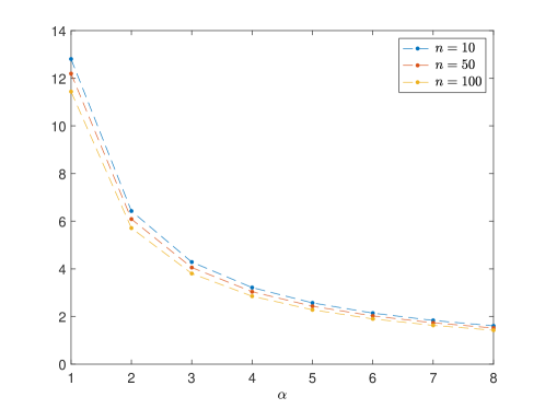
Figure 1: Percentage of increase of $R_{\max}(\hat{p}_{\alpha})$ with respect to the optimal value $R_{\max}(\hat{p}_{\rm NML})$, as a function of $\alpha$, for binary sequences of length $n=10,50,100$ and integer values of $\alpha$. The value at $\alpha=1$ corresponds to the regret of the Krichevsky-Trofimov estimator.

VI $\alpha$-NML, $\alpha$-divergence, and average $\alpha$-regret

In the previous section we showed how $\alpha$-NML improves over the Krichevsky-Trofimov estimator in terms of performance under the worst-case regret measure defined in (15), namely,

$$R_{\max}(\hat{p})=\sup_{\theta\in\Theta}\max_{x^{n}\in\mathcal{X}^{n}}\log\frac{p_{\theta}(x^{n})}{\hat{p}(x^{n})}=\sup_{\theta\in\Theta}D_{\infty}(p_{\theta}\|\hat{p}).$$ (83)

where the last equality follows from the definition of $D_{\infty}(P\|Q)$ in (19). However, for any $n$, the $\alpha$-NML still performs worse than the NML in that context, for any $\alpha<\infty$, since the NML is proven to be optimal under such a regret measure. Furthermore, it is known and it has been proved several times in different contexts (see [1] and references therein) that, under certain conditions, a mixture predictor of the form (29) is optimal under the average regret measure already defined in (12), that is,

$$R_{\rm av}(\hat{p})\triangleq\sup_{\theta\in\Theta}\mathbb{E}_{\theta}\left[\log\frac{p_{\theta}(X^{n})}{\hat{p}(X^{n})}\right]=\sup_{\theta\in\Theta}D(p_{\theta}\|\hat{p})$$ (84)

for a proper choice of the prior distribution $w(\theta)$ in (29).

Since the $\alpha$-NML predictor is an interpolation between the mixture predictor and the NML, it is natural to ask whether the $\alpha$-NML is actually optimal under some meaningful regret measure. An answer to this question comes once again from the connection between $\alpha$-NML, Sibson’s $\alpha$-mutual information, and Rényi’s $\alpha$-divergence. In fact, consider the following regret measure, defined for any $\alpha\geq 1$:

$$R_{\alpha}(\hat{p})\triangleq\sup_{\theta\in\Theta}D_{\alpha}(p_{\theta}\|\hat{p})=\sup_{\theta\in\Theta}\frac{1}{\alpha-1}\log\sum_{x^{n}\in\mathcal{X}^{n}}p_{\theta}(x^{n})\left(\frac{p_{\theta}(x^{n})}{\hat{p}(x^{n})}\right)^{\alpha-1}$$ (85)

which we call $\alpha$-regret. It follows from the definition that this measure interpolates between the average regret (84) and the worst-case regret (83), since

$$\lim_{\alpha\to 1}R_{\alpha}(\hat{p})=R_{\rm av}(\hat{p})$$ (86)

$$\lim_{\alpha\to\infty}R_{\alpha}(\hat{p})=R_{\max}(\hat{p}).$$ (87)

We first prove that, under certain conditions, $\alpha$-NML is an optimal predictor under this regret measure, when the prior $w(\theta)$ in Definition 1 is chosen properly. A similar result with a different proof is shown in [10], where the problem of the maximization of Sibson’s $\alpha$-mutual information is investigated.

Theorem 3

Assume that there exists a probability distribution $w^{*}$ on $\Theta$ such that

$$I_{\alpha}(w^{*},p_{\theta})=\sup_{w}I_{\alpha}(w,p_{\theta}).$$ (88)

Then, the $\alpha$-NML defined in (28) with prior $w^{*}$, i.e.,

$$\hat{p}_{\alpha}(x^{n})=\frac{\left\{\int_{\Theta}w^{*}(\theta)p_{\theta}^{\alpha}(x^{n})\,d\theta\right\}^{1/\alpha}}{\sum_{x^{n}}\left\{\int_{\Theta}w^{*}(\theta)p_{\theta}^{\alpha}(x^{n})\,d\theta\right\}^{1/\alpha}},$$ (89)

minimizes $R_{\alpha}(\hat{p})$ over all probability distributions on $\mathcal{X}^{n}$.

Proof:

The case for $\alpha=1$ is well known and was first proved by Gallager in [22]. We prove the theorem for $\alpha>1$, following an idea similar to Gallager’s. Let $C_{\alpha}\triangleq\sup_{w}I_{\alpha}(w,p_{\theta})$. We want to prove that

$$D_{\alpha}(p_{\theta}\|\hat{p}_{\alpha})\leq C_{\alpha}$$ (90)

for every $\theta\in\Theta$. By contradiction, suppose that there exists $\bar{\theta}\in\Theta$ such that

$$D_{\alpha}(p_{\bar{\theta}}\|\hat{p}_{\alpha})>C_{\alpha}.$$ (91)

For any $0\leq t\leq 1$, define the probability distribution

$$w^{*}_{\bar{\theta},t}=(1-t)w^{*}+t\delta_{\bar{\theta}}$$ (92)

where $\delta_{\bar{\theta}}$ is the singular distribution centered on $\bar{\theta}$. Then, we have

$$f(t)\triangleq(\alpha-1)I_{\alpha}(w^{*}_{\bar{\theta},t},p_{\theta})=\alpha\log\sum_{x^{n}}\left\{tp_{\bar{\theta}}^{\alpha}(x^{n})+(1-t)\int_{\Theta}w^{*}(\theta)p_{\theta}^{\alpha}(x^{n})\,d\theta\right\}^{1/\alpha}.$$ (93)

By the assumption that $w^{*}$ is the maximizer of $I_{\alpha}(w,p_{\theta})$, $f(t)$ is maximized at $t=0$. Taking the derivative of $f(t)$ with respect to $t$ gives

$$f^{\prime}(t)=\frac{\sum_{x^{n}}\left(p_{\bar{\theta}}^{\alpha}(x^{n})-\int_{\Theta}w^{*}(\theta)p_{\theta}^{\alpha}(x^{n})d\theta\right)\left\{\int_{\Theta}w^{*}(\theta)p_{\theta}^{\alpha}(x^{n})d\theta\right\}^{\frac{1-\alpha}{\alpha}}}{\sum_{x^{n}}\left\{tp_{\bar{\theta}}^{\alpha}(x^{n})+(1-t)\int_{\Theta}w^{*}(\theta)p_{\theta}^{\alpha}(x^{n})d\theta\right\}^{1/\alpha}}$$ (94)

Evaluating this derivative in $\lambda=0$ gives

$$f^{\prime}(0) =\frac{\sum_{x^{n}}p_{\bar{\theta}}^{\alpha}(x^{n})\left\{\int_{\Theta}w^{*}(\theta)p_{\theta}^{\alpha}(x^{n})d\theta\right\}^{\frac{1-\alpha}{\alpha}}}{\sum_{x^{n}}\left\{\int_{\Theta}w^{*}(\theta)p_{\theta}^{\alpha}(x^{n})d\theta\right\}^{1/\alpha}}-1$$ (95)

$$=\exp\big{\{}(\alpha-1)(D_{\alpha}(p_{\theta}\|\hat{p}_{\alpha})-C_{\alpha})\big{\}}-1>0.$$ (96)

This contradicts the fact that $f(t)$ is maximized at $t=0$, so we proved that $D_{\alpha}(p_{\theta}\|\hat{p}_{\alpha})\leq C_{\alpha}$ for every $\theta$. Hence,

$$R_{\alpha}(\hat{p}_{\alpha})=\max_{\theta}D_{\alpha}(p_{\theta}\|\hat{p}_{\alpha})\leq C_{\alpha}.$$ (97)

However, it is known [11] that $\min_{\hat{p}}R_{\alpha}(\hat{p})=C_{\alpha}$, which proves that $\hat{p}_{\alpha}$ with prior $w^{*}$ is indeed a minimizer of $R_{\alpha}(\hat{p})$. ∎

For the case of discrete memoryless sources, the asymptotical value of the minimal $\alpha$-regret for large $n$ was derived in [11], and its value is precisely that given in Equation (74). Since we proved that $\alpha$-NML is the optimal predictor under this regret measure, it follows that Equation (74) also gives the asymptotic $\alpha$-regret of $\alpha$-NML for the DMS case. Notice that the asymptotic difference between the $\alpha$-regret and the worst-case regret for $\alpha$-NML is exactly equal to the $W_{\alpha}(\mathcal{P})$ term in Equation (57).

It is worthwhile to give an “operational” interpretation of the regret measure defined in (85). The best setting under which this can be done is universal compression. A major reason for using the logarithmic loss as a regret measure in universal prediction problems comes from the connection that arises between prediction and compression (i.e., source coding) when this loss is used. Consider the following compression problem. Suppose that a source $S_{\theta}$ generates sequences of $n$ symbols from an alphabet $\mathcal{X}$ according to a distribution $p_{\theta}$ on $\mathcal{X}^{n}$, for some parameter $\theta\in\Theta$. A classical variable-length coding problem is to find a uniquely decodable code for the symbols in $\mathcal{X}^{n}$ that minimizes the expected length

$$L_{\mathrm{av},\theta}\triangleq\mathbb{E}_{\theta}[\ell(X^{n})]=\sum_{x^{n}\in\mathcal{X}^{n}}p_{\theta}(x^{n})\,\ell(x^{n})$$ (98)

where $\ell(x^{n})$ is the length of the codeword associated to the sequence $x^{n}$, and $X^{n}$ is distributed according to $p_{\theta}$. It is well known that the code that minimizes this quantity is any code that associates to the sequence $x^{n}$ a codeword with length $\ell(x^{n})=\log\frac{1}{p_{\theta}(x^{n})}$ (the penalty introduced when this number is not an integer turns out to be asymptotically negligible, so we omit this detail here). With such a choice, the average codeword length reaches its minimum, which is equal to the entropy of the source $H(X^{n})$.

Consider now the case where the source $S_{\theta}$ is not known in advance, and the only information that we have is that the true source parameter belongs to $\Theta$. The problem is now to design one single code for sequences in $\mathcal{X}^{n}$ that performs well for any source $S_{\theta}$ with parameter $\theta\in\Theta$. We can formulate the question as follows: if we construct our unique code in such a way that the length of the codewords is chosen to be equal to $\ell(x^{n})=\log\frac{1}{\hat{p}(x^{n})}$, what is the best distribution $\hat{p}$ that we can choose? In order to answer this question, we need to define under which metric we measure the goodness of a candidate $\hat{p}$. The chosen metric determines how much weight we give to each sequence $x^{n}$. One can then maximize this measure over all sources in $\Theta$ to get a measure that consider the worst possible source in the class.

For a fixed source $S_{\theta}$, using the optimal code (in the expected length sense described above) on a given sequence $x^{n}$ would produce a codeword of length $\log\frac{1}{p_{\theta}(x^{n})}$. Using a code constructed according to $\hat{p}$ would instead produce a codeword of length $\log\frac{1}{\hat{p}(x^{n})}$. Thus, for the sequence $x^{n}$ the difference in used bits with respect to the optimal code designed specifically for the given source is $\log\frac{1}{\hat{p}(x^{n})}-\log\frac{1}{p_{\theta}(x^{n})}=\log\frac{p_{\theta}(x^{n})}{\hat{p}(x^{n})}$. Therefore, it is natural to associate to each $x^{n}$ a cost/regret equal to $R_{\theta}(\hat{p},x^{n})=\log\frac{p_{\theta}(x^{n})}{\hat{p}(x^{n})}$, i.e., the difference in bits when encoding such a sequence. The next step is to decide how much weight to give to each sequence $x^{n}$ with respect to the others. The two approaches that we discussed before are the following.

• Giving weight to each sequence $x^{n}$ according to its probability. With this choice we obtain the average regret:

  $$R_{\mathrm{av},\theta}(\hat{p})\triangleq\mathbb{E}_{\theta}\left[\log\frac{p_{\theta}(X^{n})}{\hat{p}(X^{n})}\right]=\sum_{x^{n}}p_{\theta}(x^{n})\log\frac{p_{\theta}(x^{n})}{\hat{p}(x^{n})}=D(p_{\theta}\|\hat{p}).$$ (99)

• Considering only the sequence $x^{n}$ with the highest cost/regret. In this case we get the worst-case regret:

  $$R_{\max,\theta}(\hat{p})\triangleq\max_{x^{n}}\log\frac{p_{\theta}(x^{n})}{\hat{p}(x^{n})}=D_{\infty}(p_{\theta},\hat{p}).$$ (100)

Essentially, in the first case we are measuring the goodness of the code in terms of how many bits we waste on average, while in the second case we consider how many bits we waste in the worst case. The two measures (99) and (100) can be recognized as two extreme cases. The former averages the sequences according to their probability, without taking into account the amount of wasted bits each sequence carries. The latter considers exclusively the sequence that wastes the most number of bits, without considering how probable it is for this sequence to actually occur. A natural interpolation between these two cases is given by the Rényi divergence $D_{\alpha}(p_{\theta}\|\hat{p})$, for $1<\alpha<\infty$, since this measure takes into account all the sequences according to their probability, and at the same time gives some additional penalty to sequences with large regret. In fact, one can rewrite this measure as

$$R_{\lambda,\theta}(\hat{p})\triangleq D_{1+\lambda}(p_{\theta}\|\hat{p})=\frac{1}{\lambda}\log\sum_{x^{n}}p_{\theta}(x^{n})\exp\left(\lambda\log\frac{p_{\theta}(x^{n})}{\hat{p}(x^{n})}\right).$$ (101)

This measure is an exponential average of the regrets: the larger the value assigned to the parameter $\lambda$, the more importance is given to the number of wasted bits for each sequence $x^{n}$. It is worth noting that the exponential dependency introduced here has the same flavor as the codeword length measure that Campbell studied in [23]. However, notice that the two measures are very different. In fact, in [23] Campbell was looking for the optimal code that minimizes an alternative measure in which an exponential dependency on the codeword lengths $\ell(x^{n})$ is introduced, instead of the usual expected codeword length defined in Equation (98). In our case, instead, we are still considering the optimal code with respect to the classical expected codeword length, and the exponential dependency is on the difference in bits that the designed code uses with respect to the optimal one (in the usual expected codeword length sense). Finally, maximizing the three regret measures (99), (100) and (101) over all possible sources gives back the definitions of $R_{\rm av}(\hat{p})$, $R_{\max}(\hat{p})$ and $R_{\alpha}(\hat{p})$ seen before, where the parameter $\alpha$ in (85) and $\lambda$ in (101) are related by the equation $\alpha=1+\lambda$.

VII The role of the prior $w$ and connection to other generalizations of NML

The previous sections already made clear that the choice of the prior distribution $w$ in (28) in defining the $\alpha$-NML distribution is of fundamental importance. For example, the choice of a Dirichlet prior in (42) is what makes $\alpha$-NML almost optimal for the case of discrete memoryless sources, and the choice of the correct prior is necessary for the optimality of $\alpha$-NML under the $\alpha$-regret (85). When we discussed in Section III that the $\alpha$-NML interpolates the mixture predictors (29) and the NML (2), we assumed $w$ to be fixed and independent of $\alpha$. It turns out that if one chooses $w$ carefully as a function of $\alpha$, the $\alpha$-NML can also approximate other predictors related to the NML, which have been investigated, for example, in [15, 16].

The first predictor that we discuss is the so-called Luckiness NML [15, Section 11.3]. Let $\pi$ be a probability distribution on $\Theta$ called luckiness function: it models how confident one is that a given $\theta\in\Theta$ is the true parameter of the source. The Luckiness NML is defined as

$$\hat{p}_{\rm LNML}(x^{n})=\frac{\sup_{\theta\in\Theta}\pi(\theta)p_{\theta}(x^{n})}{\sum_{\bar{x}^{n}\in\mathcal{X}^{n}}\sup_{\theta\in\Theta}\pi(\theta)p_{\theta}(\bar{x}^{n})}.$$ (102)

It is the predictor that minimizes a regret measure realted to the worst-case regret (15), the worst-case luckiness regret, which is defined as

$$R_{\max}(\pi,\hat{p})=\max_{\theta\in\Theta}\max_{x^{n}}\frac{\pi(\theta)p_{\theta}(x^{n})}{\hat{p}(x^{n})}.$$ (103)

Notice that in [15], the author provides two different definitions of Luckiness NML. The one considered here is the one that goes under the name Luckiness NML-2 in [15]. Notice, however, that the same author points out in the more recent paper [16] that the definition that we consider here is indeed the most sensible of the two, and the one that has received more attention in the literature so far.

Another reasonable, more Bayesian, approach to define a regret measure that takes into account the luckiness $\pi(\theta)$ of a given parameter is to consider the expectation over the parameters in $\Theta$ according to $\pi$, and then the expectation over sequences distributed according to $p_{\theta}$. The result is what we may call average luckiness regret, which is formally defined as

$$R_{\rm av}(\pi,\hat{p})=\mathbb{E}_{\theta\sim\pi}\left[\mathbb{E}_{X^{n}\sim p_{\theta}}\left[\log\frac{p_{\theta}(X^{n})}{\hat{p}(X^{n})}\right]\right].$$ (104)

It is easy to prove that the predictor minimizing this regret is a mixture predictor whose weighting function is $\pi$.

Theorem 4

For a given luckiness function $\pi$, the unique predictor $\hat{p}$ that minimizes the average luckiness regret defined in (104) is

$$\hat{p}(x^{n})=\int_{\Theta}\pi(\theta)p_{\theta}(x^{n})d\theta$$ (105)

Proof:

Let $\hat{p}_{\pi}(x^{n})$ be the predictor in (105). Then, for any predictor $\hat{p}$, we can write

$$R_{\rm av}(\pi,\hat{p}) =\mathbb{E}_{\theta\sim\pi}\left[\mathbb{E}_{X^{n}\sim p_{\theta}}\left[\log\frac{p_{\theta}(X^{n})}{\hat{p}(X^{n})}\right]\right]$$ (106)

$$=\mathbb{E}_{\theta\sim\pi}\left[\mathbb{E}_{X^{n}\sim p_{\theta}}\left[\log\frac{p_{\theta}(X^{n})}{\hat{p}_{\pi}(X^{n})}+\log\frac{\hat{p}_{\pi}(X^{n})}{\hat{p}(X^{n})}\right]\right]$$ (107)

$$=R_{\rm av}(\pi,\hat{p}_{\pi})+\mathbb{E}_{\theta\sim\pi}\left[\mathbb{E}_{X^{n}\sim p_{\theta}}\left[\log\frac{\hat{p}_{\pi}(X^{n})}{\hat{p}(X^{n})}\right]\right]$$ (108)

$$=R_{\rm av}(\pi,\hat{p}_{\pi})+D(\hat{p}_{\pi}\|\hat{p})$$ (109)

where in the last step we used the definition of the Kullback-Leibler divergence (18). The theorem follows from the fact that the KL divergence is always non-negative, and it is equal to zero if and only if $\hat{p}_{\pi}=\hat{p}$. ∎

A possible interpolation between the luckiness NML defined in (102) and the mixture predictor in (105) is again given by $\alpha$-NML of Equation (28), if one chooses the proper prior distribution $w$. In fact, for any given $\alpha\geq 1$, one can take the tilted prior distribution

$$w(\theta)=\frac{\pi(\theta)^{\alpha}}{\int_{\Theta}\pi(\theta)^{\alpha}d\theta}$$ (110)

provided that the integral in the denominator converges. With such a choice of prior, the $\alpha$-NML becomes

$$\hat{p}_{\alpha}(x^{n}) =\frac{\left\{\int_{\Theta}w(\theta)\,p_{\theta}^{\alpha}(x^{n})\,d\theta\right\}^{1/\alpha}}{\sum_{x^{n}}\left\{\int_{\Theta}w(\theta)\,p_{\theta}^{\alpha}(x^{n})\,d\theta\right\}^{1/\alpha}}$$ (111)

$$=\frac{\left\{\int_{\Theta}(\pi(\theta)\,p_{\theta}(x^{n}))^{\alpha}\,d\theta\right\}^{1/\alpha}}{\sum_{x^{n}}\left\{\int_{\Theta}(\pi(\theta)\,p_{\theta}(x^{n}))^{\alpha}\,d\theta\right\}^{1/\alpha}}.$$ (112)

For convenience, we can call this predictor luckiness $\alpha$-NML. However, it is important to note that this predictor is not something different from the already defined $\alpha$-NML. In fact, it is simply a particular instance of that same predictor, where one chooses a particular prior distribution $w$ – in this case, it is the one in Equation (110). In this sense, the $\alpha$-NML is able to link the standard NML and the luckiness NML under the same, more general, object. By taking $\alpha=1$, one retrieves the mixture predictor in (105), while in the limit $\alpha\to\infty$, one gets the luckiness NML that is defined in (102).

Similarly to the case of the $\alpha$-regret of Equation (85), there also exists an interpolation between the worst-case luckiness regret in (103) and the average luckiness regret in (104) for which the luckiness $\alpha$-NML is the optimal predictor. In fact, consider the luckiness regret defined for any $\alpha\geq 1$ by

$$R_{\alpha}(\pi,\hat{p})=\frac{1}{\alpha-1}\log\mathbb{E}_{\theta\sim\pi_{\alpha}}\left[\mathbb{E}_{X^{n}\sim p_{\theta}}\left[\left(\frac{p_{\theta}(X^{n})}{\hat{p}(X^{n})}\right)^{\alpha-1}\right]\right]$$ (113)

where

$$\pi_{\alpha}(\theta)=\frac{\pi(\theta)^{\alpha}}{\int_{\Theta}\pi(\bar{\theta})^{\alpha}d\bar{\theta}}.$$ (114)

Notice that the exponent of $\alpha$ inside the expectation is the same as in (85), as well as the normalization factor $\frac{1}{\alpha-1}\log$ in front. However, there is an important difference on how the interpolation between the average and the worst-case is handled in the two cases. The interpolation of $R_{\alpha}$ in the standard case acts only on how the sequences $x^{n}$ are considered, since in both (83) and (84) there is a maximization over $\theta$. In the luckiness case, instead, the interpolation also occurs on how the parameters in $\Theta$ are counted. In fact, in the worst-case luckiness regret (103) there is a maximization over $\theta$, while in the average luckiness regret (104) there is an expectation according to $\pi$. The way this interpolation is handled in (113) is through an expectation over a tilted version of the luckiness function $\pi$, which equals $\pi$ when $\alpha=1$, and it assigns probability one to the maximal $\theta$ when $\alpha\to\infty$. The optimal predictor for the luckiness $\alpha$-regret is the luckiness $\alpha$-NML.

Theorem 5

For any given $\alpha\geq 1$ and any given luckiness function $\pi$ over $\Theta$, the luckiness $\alpha$-NML defined in (112) with prior distribution $w$ taken as in (110), minimizes $R_{\alpha}(\pi,\hat{p})$ over all probability distributions on $\mathcal{X}^{n}$, under the assumption that the prior distribution converges, i.e., if

$$\int_{\Theta}\pi(\theta)^{\alpha}d\theta<\infty.$$ (115)

Proof:

Notice that one can rewrite (113) as

$$R_{\alpha}(\pi,\hat{p})=D_{\alpha}(\pi_{\alpha}\times p_{\theta}\|\pi_{\alpha}\times\hat{p})$$ (116)

where we used the definition of Rényi divergence as in Equation (17). Thanks to [9, Equation (32)], it follows that the minimum regret over all predictors $\hat{p}$ satisfies

$$\min_{\hat{p}}R_{\alpha}(\pi,\hat{p})=\min_{\hat{p}}D_{\alpha}(\pi_{\alpha}\times p_{\theta}\|\pi_{\alpha}\times\hat{p})=I_{\alpha}(\pi_{\alpha},p_{\theta}).$$ (117)

Furthermore, one can check by substituting the definition of luckiness $\alpha$-NML (112) with prior $\pi_{\alpha}$ into (113), that the regret of the luckiness $\alpha$-NML is equal to

$$R_{\alpha}(\pi,\hat{p}_{\alpha})=I_{\alpha}(\pi_{\alpha},p_{\theta}).$$ (118)

From (117) and (118) it follows that the luckiness $\alpha$-NML minimizes the regret. ∎

Alternatively, one could define a different average luckiness regret measure such as

$$\tilde{R}_{\rm av}(\pi,\hat{p})=\max_{\theta\in\Theta}\mathbb{E}_{X^{n}\sim p_{\theta}}\left[\log\frac{\pi(\theta)p_{\theta}(X^{n})}{\hat{p}(X^{n})}\right].$$ (119)

Then, a simple interpolation between this regret and (103) is

$$R_{\alpha}(\pi,\hat{p})=\sup_{\theta\in\Theta}\frac{1}{\alpha-1}\log\mathbb{E}_{X^{n}\sim p_{\theta}}\left[\left(\frac{\pi(\theta)p_{\theta}(X^{n})}{\hat{p}(X^{n})}\right)^{\alpha-1}\right]$$ (120)

which is strongly related to the $\alpha$-regret in Equation (85). In fact, one can prove a result similar to Theorem 3 for this regret measure. In this context, it can be used to show that there exists a distribution $w^{*}(\theta)$ on $\Theta$ such that the $\alpha$-NML defined in (28), with prior equal to

$$w(\theta)=\frac{w^{*}(\theta)\pi^{\alpha}(\theta)}{\int_{\Theta}w^{*}(\bar{\theta})\pi^{\alpha}(\bar{\theta})d\bar{\theta}}$$ (121)

is the predictor that minimizes (120).

An important, particular case of the Luckiness NML studied above is the Conditional NML. Its definition follows directly from that of Luckiness NML as in (102), where the luckiness function $\pi(\theta)$ is taken to be equal to

$$\pi(\theta)=\frac{p_{\theta}(\bm{x}_{0})}{\int_{\Theta}p_{\bar{\theta}}(\bm{x}_{0})d\bar{\theta}}$$ (122)

for some fixed sequence $\bm{x}_{0}\in\mathcal{X}^{m}$, for some $m\geq 1$. This distribution can be interpreted as a posterior distribution over the parameter space $\Theta$ given the sequence $\bm{x}_{0}$, with the prior over $\Theta$ being uniform. The sequence $\bm{x}_{0}$ is understood to be a sequence previously generated by the source, so that we design our predictor conditioned on this already-known sequence. Since the Conditional NML is a special case of Luckiness NML, all the results obtained above for the luckiness $\alpha$-NML can be derived also for this particular case, where $\pi(\theta)$ is taken as in (122).

VIII Conclusion

In this paper, we introduced a new class of general predictors dependent on a real parameter $\alpha\geq 1$, with the objective of finding alternative predictors with good finite-length performance compared to the optimal NML, avoiding at the same time some of the impractical drawbacks of the latter. The idea for this class of predictors comes from the connection that exists between the worst-case regret achieved by the NML predictor, and Sibson’s $\alpha$-mutual information. Furthermore, we showed that for the popular family of discrete memoryless sources, one is able to derive some simple formulas to compute the probabilities estimated by the new class of predictors, when the parameter $\alpha$ is a positive integer. Furthermore, from a complementary point of view, we proved the optimality of $\alpha$-NML under some alternative regret measures linked to Rényi divergence and Sibson’s $\alpha$-mutual information that interpolate between the well-known average and worst-case regret. Finally, we analyzed the role of the prior distribution $w$ on the parameter space in the definition of $\alpha$-NML, and how proper choices of this prior connect $\alpha$-NML to other generalizations of NML such as Luckiness NML and Conditional NML.

References

- [1] N. Merhav and M. Feder, “Universal prediction,” IEEE Trans. Inf. Theory, vol. 44, no. 6, pp. 2124–2147, 1998.
- [2] J. Ziv and A. Lempel, “A universal algorithm for sequential data compression,” IEEE Trans. Inf. Theory, vol. 23, no. 3, pp. 337–343, 1977.
- [3] F. Willems, Y. Shtarkov, and T. Tjalkens, “The context-tree weighting method: basic properties,” IEEE Trans. Inf. Theory, vol. 41, no. 3, pp. 653–664, 1995.
- [4] Q. Xie and A. Barron, “Asymptotic minimax regret for data compression, gambling, and prediction,” IEEE Trans. Inf. Theory, vol. 46, no. 2, pp. 431–445, 2000.
- [5] Y. Fogel and M. Feder, “Universal learning of individual data,” in Proc. 2019 IEEE Int. Symp. Inf. Theory (ISIT), 2019, pp. 2289–2293.
- [6] F. E. Rosas, P. A. M. Mediano, and M. Gastpar, “Learning, compression, and leakage: Minimising classification error via meta-universal compression principles,” in Proc. 2020 IEEE Inf. Theory Workshop (ITW), 2021.
- [7] Y. M. Shtarkov, “Universal sequential coding of single messages,” Problems Inform. Transmission, vol. 23, no. 3, pp. 175–186, 1987.
- [8] R. Krichevsky and V. Trofimov, “The performance of universal encoding,” IEEE Trans. Inf. Theory, vol. 27, no. 2, pp. 199–207, 1981.
- [9] S. Verdú, “-mutual information,” in Proc. 2015 IEEE Inf. Theory Appl. Workshop (ITA), 2015.
- [10] C. Cai and S. Verdú, “Conditional Rényi divergence saddlepoint and the maximization of -mutual information,” Entropy, vol. 21, no. 10, 2019.
- [11] S. Yagli, Y. Altuğ, and S. Verdú, “Minimax Rényi redundancy,” IEEE Trans. Inf. Theory, vol. 64, no. 5, pp. 3715–3733, 2018.
- [12] T. van Erven and P. Harremoës, “Rényi divergence and Kullback-Leibler divergence,” IEEE Trans. Inf. Theory, vol. 60, no. 7, pp. 3797–3820, 2014.
- [13] L. Davisson, “Universal noiseless coding,” IEEE Trans. Inf. Theory, vol. 19, no. 6, pp. 783–795, 1973.
- [14] J. Rissanen, “Complexity of strings in the class of Markov sources,” IEEE Trans. Inf. Theory, vol. 32, no. 4, pp. 526–532, 1986.
- [15] P. D. Grünwald, The minimum description length principle. Cambridge, MA: MIT Press, 2007.
- [16] P. Grünwald and T. Roos, “Minimum description length revisited,” International Journal of Mathematics for Industry, vol. 11, no. 01, 2019.
- [17] A. Barron, T. Roos, and K. Watanabe, “Bayesian properties of normalized maximum likelihood and its fast computation,” in Proc. 2014 IEEE Int. Symp. Inf. Theory (ISIT), 2014, pp. 1667–1671.
- [18] N. Cesa-Bianchi and G. Lugosi, Prediction, learning, and games. Cambridge, United Kingdom: Cambridge University Press, 2006.
- [19] H. Jeffreys, “An invariant form for the prior probability in estimation problems,” Proceedings of the Royal Society A, vol. 186, pp. 453–461, 1946.
- [20] H. Alzer and C. Berg, “Some classes of completely monotonic functions, II,” The Ramanujan Journal, vol. 11, no. 2, pp. 225–248, 2006.
- [21] M. Abramowitz and I. A. Stegun, Handbook of mathematical functions with formulas, graphs, and mathematical tables. Gaithersburg, MD: National Bureau of Standards, 1970.
- [22] R. G. Gallager, “Source coding with side information and universal coding.” [Online]. Available: https://web.mit.edu/gallager/www/papers/paper5.pdf
- [23] L. Campbell, “A coding theorem and Rényi’s entropy,” Information and Control, vol. 8, no. 4, pp. 423–429, 1965.