Take the $A$-Metric: Interpretations of Some Known Solutions of Einstein’s Vacuum Field Equations

Laboratory of Photonics, Physics Unit, Tampere University, FI-33720 Finland *email: charles.robson@tuni.fi

In this work, we present a new interpretation of the only static vacuum solution of Einstein’s field equations with planar symmetry, the Taub solution. This solution is a member of the $AIII$ class of metrics, along with the type D Kasner solution. Various interpretations of these solutions have been put forward previously in the literature, however, some of these interpretations have suspect features and are not generally considered physical. Using a simple mathematical analysis, we show that a novel interpretation of the Taub solution is possible and that it naturally emerges from the radial, near-singularity limit of negative-mass Schwarzschild spacetime. A new, more transparent derivation is also given showing that the type D Kasner metric can be interpreted as a region of spacetime deep within a positive-mass Schwarzschild black hole. The dual nature of this class of $A$-metrics is thereby demonstrated.

Keywords: General relativity; Einstein’s vacuum field equations; Schwarzschild metric; negative mass; Kasner solution; Taub solution.

1 Introduction

Over the previous century, a vast number of solutions of Einstein’s field equations have been discovered [1, 2, 3, 4, 5, 6, 7]. During this same period, however, a much smaller number of agreed-upon physical interpretations of these solutions have been established [8, 9, 10, 11, 12]. Some spacetime solutions have clear interpretations: there is a consensus, for example, that certain metrics describe black holes, gravitational waves, and cosmologies, but other solutions have much more mysterious origins – some can be interpreted as describing local regions of realistic spacetimes, some indeed have multiple feasible readings, and others currently have none at all [8]. Dealing with the protean nature of solutions, a by-product of the general covariance of the field equations, can require subtle methods such as obscure coordinate transformations [13].

Hidden within the structure of general relativity, there are doubtless undiscovered solutions describing novel spacetime configurations with relevance and importance today. It is nevertheless arguable that the immediate task is to interpret those solutions that have already been found through many years of great effort [1, 8, 2]. It is a pressing task then, as it has been since the early days of general relativity, to find reasonable and useful interpretations of all its solutions and to reassess those with doubtful features.

In this paper, we make a contribution to this task by presenting a new interpretation of a class of solutions known as the $AIII$-metrics [8, 2]. Previous explanations of the physics described by these solutions contain questionable properties, including fine-tuned parameters [8]. We argue that our new interpretation is by far the most natural yet suggested, relating as it does to a local region of the Schwarzschild solution with finite mass parameter. Our result is found using only simple mathematical analysis.

The $AIII$-metrics are a subclass of the more general $A$-metrics family, the latter classified by Ehlers and Kundt in 1962 [2]. Each subclass of the $A$-metrics family is characterised by a 2-space curvature parameter. Depending on the choice of this parameter, one finds the well-known Schwarzschild solution ($AI$), a solution with a negative-Gaussian-curvature hypersurface ($AII$), capable of describing the gravitational field produced by a tachyon [14], or the $AIII$-metrics; in this paper, we focus purely on the final subclass, as the different interpretations and geometrical features present (including a curvature singularity) in these vacuum solutions make them an interesting topic of study.

As has been previously stated [8], “most solutions of Einstein’s equations may have no satisfactory interpretation as global models of realistic physical situations at all. On the other hand, locally, many may reasonably represent particular regions of realistic space-times”. Consistent with this point of view, it is local spacetime regions that are the focus of this paper.

In Sec. 2, we present our results reinterpreting the $AIII$-metrics as local regions of Schwarzschild spacetime. Sec. 3 contains a critical survey of previous readings of the $AIII$-metrics, putting forward the case that ours is the most natural, avoiding as it does characteristics that render other interpretations unphysical or obscure. Sec. 4 contains a summary of the paper. Several appendices contain useful coordinate transformations, a discussion of how the Kasner metric relates to the physics inside a black hole, and a description of the geometry connected with our results.

2 Results

The family of vacuum spacetimes known as the $A$-metrics will be the focus of this work and is given by [2, 8]

$$ds^{2}=-\left(\epsilon-\frac{2M}{r}\right)dt^{2}+\left(\epsilon-\frac{2M}{r}\right)^{-1}dr^{2}+r^{2}\frac{2d\zeta d\bar{\zeta}}{\left(1+\epsilon\zeta\bar{\zeta}/2\right)^{2}}.$$ (1)

These are a rich and intriguing generalisation of the Schwarzschild solution, describing different spacetimes depending on the value of parameter $\epsilon$ (which can be $+1$, $-1$ or $0$); fixing the value of $\epsilon$ determines the Gaussian curvature of the hypersurface on which $t$ and $r$ are constant. Setting $\epsilon=1$ produces the $AI$-metric, i.e. the Schwarzschild solution. $M$ is an arbitrary, continuous parameter and $\bar{\zeta}$ is the complex conjugate of $\zeta$. Relevant coordinate ranges will be discussed below.

In this paper, we restrict our attention to the AIII-metrics, which emerge setting $\epsilon=0$ in Eq. (1). Performing the coordinate transformation $\zeta=\rho\mathrm{exp}(i\phi)/\sqrt{2}$ with $\phi\in[0,2\pi)$ then gives

$$ds^{2}=\frac{2M}{r}dt^{2}-\frac{r}{2M}dr^{2}+r^{2}\left(d\rho^{2}+\rho^{2}d\phi^{2}\right).$$ (2)

Due to the curvature singularity at $r=0$, it is appropriate to constrain the value of the coordinate as $r>0$. The line element (2) has been interpreted in various different ways in the literature, as will be discussed in detail in Sec. 3.

When $M$ is positive and finite, Eq. (2) describes the polar spacetime deep within a Schwarzschild black hole of finite positive mass. What has not been noted before, is that when $M$ is negative and finite, metric (2) describes the small-$r$, polar region of negative-finite-mass Schwarzschild spacetime. By “polar spacetime” we mean that the spacetime is restricted to $\theta\ll 1$, where $\theta$ is the polar angle of the Schwarzschild coordinate system (see below), and “deep within” a Schwarzschild black hole denotes $r\ll 2M$, where $r$ is the radial Schwarzschild coordinate. Note that the negative-mass case has no event horizon and by “small-$r$” we signify $r\ll 2|M|$, with $2|M|$ the characteristic length scale of the system. As there is no horizon for the negative-mass Schwarzschild spacetime, it contains a naked singularity; for a discussion of the physical feasibility of this configuration, see Ref. [15] and references therein. For the rest of this paper, we refer to the zone $\theta\ll 1$, $r\ll 2|M|$ as the deep-radial region.

New derivations supporting the above statements are now given. Starting from the Schwarzschild solution with $M>0$ [5],

$$ds^{2}=-\left(1-\frac{2M}{r}\right)dt^{2}+\left(1-\frac{2M}{r}\right)^{-1}dr^{2}+r^{2}\left(d\theta^{2}+\mathrm{sin}^{2}\theta d\phi^{2}\right),$$ (3)

and taking the limits $r\ll 2M$ and $\theta\ll 1$, one can see that the term $1-2M/r$ can be approximated by $-2M/r$ and that $\mathrm{sin}^{2}\theta\approx\theta^{2}+\mathcal{O}(\theta^{4})$. Because $\theta\ll 1$, we discard the $\mathcal{O}(\theta^{4})$ term in the Taylor series of $\mathrm{sin}^{2}\theta$, leading to the metric

$$ds^{2}\approx\frac{2M}{r}dt^{2}-\frac{r}{2M}dr^{2}+r^{2}\left(d\theta^{2}+\theta^{2}d\phi^{2}\right),\hskip 14.22636ptM>0.$$ (4)

In general relativity, the coordinates have no intrinsic physical meaning and must be interpreted [3]. We are therefore free to interpret $\theta$ in Eq. (4) as a dimensionless radial coordinate, which, together with azimuth $\phi$, defines a two-dimensional polar coordinate system. This coordinate reinterpretation after taking the limits $r\ll 2M$ and $\theta\ll 1$ above is natural, as the line element section $d\theta^{2}+\theta^{2}d\phi^{2}$ from (4) is intrinsically flat. A relabelling $\theta\rightarrow\rho$ in (4) yields the $AIII$-metric (2) with $M>0$. The $t$ coordinate spans the real line.

In case the reinterpretation of coordinates above seems obscure, all we have done is to approximate the surface of a two-sphere as locally Euclidean (when $\theta\ll 1$ holds). We are free to do this as the two-sphere $S^{2}$ is a manifold and so, by definition, locally “looks like” $\mathbb{R}^{2}$ [5]. If one chose to, one could “sew together” these pieces which locally resemble $\mathbb{R}^{2}$ in order to reconstruct $S^{2}$ [4]. Each of us unconsciously makes this approximation every day – the Earth appears locally flat as one walks on its surface even though it is of course globally (roughly) spherical.

An important point concerning the $\theta\ll 1$ constraint is that it does not pick out any special pole in Schwarzschild spacetime, thereby breaking the solution’s spherical symmetry [16]. The choice of the origin of the $\theta$ coordinate is arbitrary (in other words, there is no “north pole” of a Schwarzschild black hole) and fixing $\theta\ll 1$ simply restricts the geometry to a thin cone of the spacetime, centred around any radial line. The additional constraint $r\ll 2M$ then “places” this cone behind the horizon. Note that the coordinate $r$ is timelike in the deep-radial region for $M>0$ and this must be kept in mind when visualising the spacetime. See Appendix A for details.

The $AIII$-metric with $M>0$ can thus be interpreted as a local description of Schwarzschild spacetime in the limits $r\ll 2M$ and $\theta\ll 1$, using a simple approximation.

The preceding analysis held for $M>0$. In the case of the Schwarzschild solution with negative mass $M<0$, the metric can be written as

$$ds^{2}=-\left(1+\frac{2|M|}{r}\right)dt^{2}+\left(1+\frac{2|M|}{r}\right)^{-1}dr^{2}+r^{2}\left(d\theta^{2}+\mathrm{sin}^{2}\theta d\phi^{2}\right).$$ (5)

Taking the limits $r\ll 2|M|$ and $\theta\ll 1$, the term $1+2|M|/r$ can be approximated by $2|M|/r$, giving

$$ds^{2}\approx-\frac{2|M|}{r}dt^{2}+\frac{r}{2|M|}dr^{2}+r^{2}\left(d\theta^{2}+\theta^{2}d\phi^{2}\right).$$ (6)

Substituting $M=-|M|$ into metric (6) and relabelling $\theta\rightarrow\rho$ as before then yields

$$ds^{2}\approx\frac{2M}{r}dt^{2}-\frac{r}{2M}dr^{2}+r^{2}\left(d\rho^{2}+\rho^{2}d\phi^{2}\right),\hskip 14.22636ptM<0.$$ (7)

Metrics (4) and (7) are therefore just the positive- and negative-“mass” branches of the $AIII$-metrics (2). The coordinate domain of $\phi$ is the same throughout: $\phi\in[0,2\pi)$. Of course, due to the domain constraints introduced, in Eq. (2) the upper limit of the $\rho$ coordinate must be restricted to a small, finite number $\rho_{0}$, i.e. $\rho\in[0,\rho{{}_{0}}\ll 1]$, and the $r$ coordinate has to obey $0<r\ll 2|M|$.

Another way to compare geometries is via the use of curvature invariants. The following scalar invariants, defined using the metric tensor, are equal for both the ($M>0$) $AIII$- and Schwarzschild metrics: the Ricci scalar ($R=0$) and Kretschmann scalar ($K=48M^{2}/r^{6}$) [5, 18]. Another invariant, the Karlhede scalar $K_{2}$ [19, 20], differs globally over $r$: for Schwarzschild spacetime, $K_{2}=720M^{2}(r-2M)/r^{9}$, whereas for the $AIII$ class of solutions, $K_{2}=-1440M^{3}/r^{9}$. It is clear however that in the limit $r\ll 2M$ the Karlhede scalars approximately match, as expected. The matching becomes closer as the singularity is approached. This argument can be easily adapted to the $M<0$ case, showing a matching there too.

3 Discussion

There exist in the literature several different interpretations of the $AIII$-metrics, with various properties. We introduce and discuss them in this section, comparing them critically with ours.

Applying a simple coordinate transformation to the $AIII$-metric (2) for the case $M>0$ demonstrates that it is the type D vacuum Kasner solution [8] (for more details on this metric, and the vacuum Bianchi I class of solutions to which it belongs, see Refs. [21, 23, 13, 22]). This solution can be interpreted as a description of a certain anisotropic cosmology beginning with a (spacelike) big bang-type singularity [8]. This “cosmological picture” (as we refer to it from here on) does not clash with the interpretation of the Kasner solution as a description of the deep-radial region of a Schwarzschild black hole. Both are valid, as we now show.

Performing the aforementioned coordinate transformation (see Appendix B for details) on the $M>0$ $AIII$-metric (2) yields the line element

$$ds^{2}=-d\tau^{2}+\tau^{-2/3}dz^{2}+\tau^{4/3}(dx^{2}+dy^{2}).$$ (8)

The cosmological picture asserts that the type D vacuum Kasner solution describes a spacetime originating in a spacelike singularity at the origin $\tau=0$ [equivalent to $r=0$ in Eq. (2)]. The coordinate origin $r=0$ is also a spacelike singularity in Schwarzschild spacetime, hence both interpretations account for this feature. The fact that the coordinate $t$ is spacelike and $r$ is timelike for the $AIII$-metric (2) with $M>0$ is interpreted in the cosmological picture by treating $r$ as related to a global time coordinate [i.e. $\tau$ in Eq. (8)] characterising the evolution of the spacetime, and by taking $t$ as proportional to a spatial dimension [i.e. $z$ in Eq. (8)]. The deep-radial interpretation also explains these features, as the Schwarzschild coordinates $t$ and $r$ are spacelike and timelike, respectively, behind the horizon.

In the cosmological picture, the vacuum spacetime (after its “big bang” at $\tau=0$) expands uniformly in two directions whilst contracting in the remaining spatial dimension. As was shown in Sec. 2, the deep-radial region of Schwarzschild spacetime can be approximated by a flat disk for $(t,r)=$constant. If one looks at the geometry of this disk, one can see how it matches the geometry in the cosmological picture, supplying a parallel viewpoint. Let us focus our attention on one piece of metric (4), specifically

$$ds^{2}\big{|}_{\left(\theta,\phi\right)}=r^{2}\left(d\theta^{2}+\theta^{2}d\phi^{2}\right),$$ (9)

where the notation $ds^{2}\big{|}_{\left(\theta,\phi\right)}$ denotes the $\left(\theta,\phi\right)$ sector of the line element. Our approximation demands $\theta\ll 1$, so we restrict the coordinate $\theta$ to the range $\theta\in[0,\theta_{0}]$, where $\theta_{0}\ll 1$. As mentioned earlier, the symbol $\theta$ is open to interpretation, as are all coordinates in general relativity, and the part of the metric (9) in brackets defines a flat disk of radius $\theta_{0}$, spanned by dimensionless radial coordinate $\theta$ and azimuthal coordinate $\phi$. As can be read directly from (9), the dimensionless disk grows with coordinate $r$. This “growth” of the disk follows directly from conical geometry (see Appendix A).

It is instructive to compare the Penrose diagram of the type D Kasner solution with that of the inside of a Schwarzschild black hole, as they show the same near-singularity structure. The condition $r\ll 2M$ for the Schwarzschild spacetime is equivalent to $\tau\ll 4M/3$ in Kasner coordinate, therefore, the small-$\tau$ sector of the Kasner Penrose diagram (see left side of Figure 1) matches the $r\ll 2M$ sector of the Schwarzschild Penrose diagram; in a similar way, the conformal diagram of the Taub solution (right side of Figure 1) for small-$\tilde{z}$ matches that of negative-mass Schwarzschild for $r\ll 2|M|$ [8].

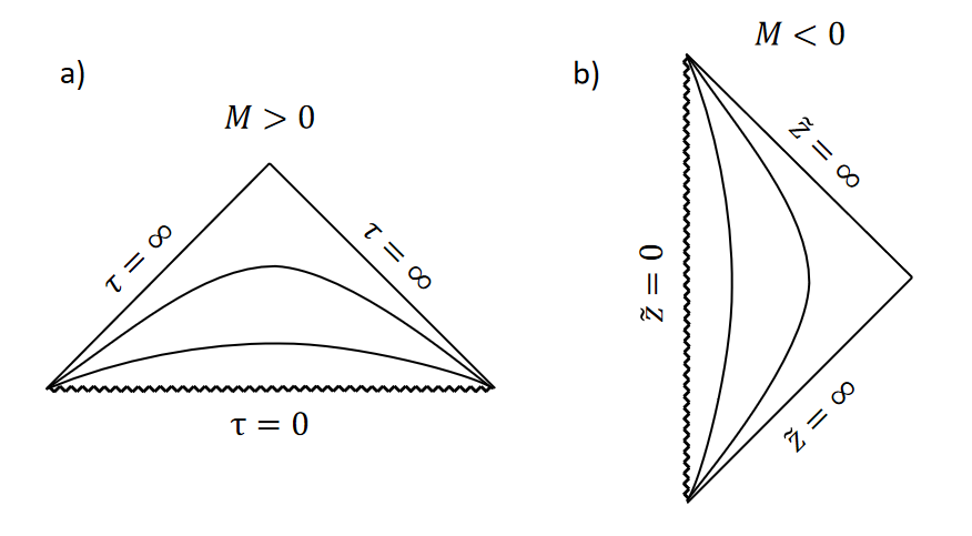
Figure 1: Conformal (Penrose) diagrams for the $AIII$ metrics: a) Kasner solution; b) Taub solution.

This provides an example of an interesting feature of general relativity, namely that a single metric can describe apparently unrelated physical phenomena: in this case, both the birth and expansion of a universe and the spacetime deep within a black hole. To reiterate, the cosmological picture and the deep-radial Schwarzschild interpretation of the ($M>0$) $AIII$-metric (2) are both valid and not mutually exclusive.

Let us now discuss the case of negative parameter, $M<0$. A simple coordinate transformation (see Appendix C) shows that metric (7) is in fact the Taub solution, the only static vacuum solution with planar symmetry [8, 30, 31]; this solution has a timelike singularity at $r=0$.

There have been numerous attempts to physically interpret the $AIII$-metric for $M<0$ [Eq. (7)], but, as stated in Ref. [8], “a totally satisfactory interpretation of this simple static metric has still not been found”. One of the reasons for this past difficulty may have been a too-strong focus on obtaining a global interpretation of the solution, which is problematic due to its planar symmetry. Our approach is local in nature.

Previously-published suggestions include one arguing that the origin at $r=0$ describes a static infinite plane source that repels timelike geodesics [17, 10, 32]. Another is that this spacetime is a description of the external region sourced by an infinite line of fixed negative gravitational mass per unit length [8]; yet another interpretation is that the spacetime describes the exterior region of a semi-infinite rod source, again with a specific, fixed negative mass density [33]. A reading of the metric as modelling the field due to a null particle [34] has also been published but has been argued to be incorrect [35, 33].

Our new interpretation removes all need for unusual sources (except for negative mass) and fine-tuned parameters, and in addition it explains the behaviour of test particles (timelike geodesics) and null rays as they approach the singularity. The behaviour of geodesics in the Taub spacetime has been studied by Bedran et al. [17]. They found that massive particles cannot reach the singularity, independent of initial conditions, but that massless particles can attain the singularity when falling perpendicular to the plane of symmetry. The behaviour of geodesics in negative-mass Schwarzschild spacetime has also previously been studied [36, 37], demonstrating the same qualitative behaviour: test particles are repulsed from the singularity but a radially-infalling ray of light can reach it in finite time. The consistent behaviour of geodesics in both Taub and negative-mass Schwarzschild spacetimes is not a coincidence, as the former describes a local region of the latter.

Our interpretation also explains a hitherto mysterious feature of the behaviour of test particles in Taub spacetime, pointed out by Bonnor [10]: the proper distance between two test particles decreases as the singularity is approached. There is no apparent reason for this if the singular source were a plane, however, our new interpretation resolves this: as the $r=0$ singularity is approached, two neighbouring paths will indeed begin to coalesce for negative-mass Schwarzschild spacetime, as the “Taub plane” itself (the base of the cone in Appendix A) shrinks.

Another piece of evidence against a negative-mass planar source seeding Taub spacetime, noted previously [8, 10], is that general relativity does not seem to predict a corresponding positive-mass planar source, making the negative-mass source suspect. Our interpretation resolves this apparent discrepancy, as both positive- and negative-mass sources are provided by the $M>0$ and $M<0$ Schwarzschild solutions, respectively. This pleasing symmetry in our new reading of the $AIII$-metrics illuminates the previously-noted “dual” nature [17] of the Taub and Kasner solutions.

As has been pointed out by other authors, the Kasner and Taub solutions also emerge from infinite-mass limits of Schwarzschild spacetime [17, 2, 34, 39, 7, 38]. A simple proof of this fact was given in Ref. [38], which we reproduce here. The following solution of Einstein’s field equations,

$$ds^{2}=-\left(K-\frac{2M}{r}\right)dt^{2}+\left(K-\frac{2M}{r}\right)^{-1}dr^{2}+r^{2}\left(d\widetilde{\theta}^{2}+\mathrm{cos}^{2}\left(\sqrt{K}\widetilde{\theta}\right)d\phi^{2}\right),$$ (10)

has a limit to Schwarzschild spacetime when $K\rightarrow 1$ and a limit to Taub (Kasner) spacetime when $K\rightarrow 0$ and $M<0$ ($M>0$). The symbol $K$ now represents a parameter taking an arbitrary value and no longer denotes the Kretschmann invariant as it did in Sec. 2. Using the coordinate transformations

$$R\equiv r/\sqrt{K},\qquad T\equiv t\sqrt{K},\qquad\overline{\theta}\equiv\widetilde{\theta}\sqrt{K},\qquad\overline{\phi}\equiv\phi\sqrt{K},$$ (11)

metric (10) becomes

$$ds^{2}=-\left(1-\frac{2\widetilde{M}}{R}\right)dT^{2}+\left(1-\frac{2\widetilde{M}}{R}\right)^{-1}dR^{2}+R^{2}\left(d\overline{\theta}^{2}+\mathrm{cos}^{2}\overline{\theta}d\overline{\phi}^{2}\right),$$ (12)

which is the Schwarzschild solution with mass parameter $\widetilde{M}=M/(K^{3/2})$. As is clear in these new coordinates, for positive $M$, the limit $K\rightarrow 0$ corresponds to the limit $\widetilde{M}\rightarrow\infty$. For negative $M$, the limit $K\rightarrow 0$ corresponds to $\widetilde{M}\rightarrow-\infty$.

We argue that the deep-radial interpretations of the Kasner and Taub metrics are considerably more natural than the ones suggested by the above limits, as the former avoid the pathologies of infinite positive or negative mass, which are evidently unphysical.

In the future, it is hoped that other simple physical pictures for solutions to Einstein’s field equations may be found, using local techniques such as ours when global descriptions are lacking. It would be interesting to investigate whether local approaches are also useful in finding new interpretations of other $A$-metrics and of generalisations thereof with multiple parameters.

4 Conclusions

We have put forward a new interpretation of a member of the $AIII$ class of metrics, namely the plane symmetric static Taub solution. A new, more transparent derivation of the relationship between the region deep within a Schwarzschild black hole and the type D Kasner solution is also presented, highlighting the “duality” between Kasner and Taub solutions. These solutions to Einstein’s field equations in vacuum have been known for decades, however, for the Taub case, a natural, agreed-upon physical description has been lacking. We show that, depending on the sign of parameter $M$ (the only parameter in the solution), the $AIII$-metrics describe either a local region deep inside a Schwarzschild black hole or a sector of negative-mass Schwarzschild spacetime. These simple, dual descriptions are compared critically with previously published ones.

Acknowledgments: The authors wish to thank Kexin Wang for his help with the figures.

Appendix A: Illustration of the geometries

If one fixes the variables $t$ and $r$ in metric (4) to constants, $t=t_{0}$ and $r=r_{0}$, the line element reduces to

$$ds^{2}={r_{0}}^{2}\left(d\theta^{2}+\theta^{2}d\phi^{2}\right).$$ (13)

We now show that this is a simple example of conical geometry, with the first fundamental form (13) describing the base of a cone for small apex angle, thereby proving our assertion in the main text that $\theta$ can be treated as a dimensionless radial coordinate after enforcing the constraint $\theta\ll 1$, and making the geometry easier to visualise.

A right circular cone can fit into a spherical coordinate system as shown in Figure 2; the Schwarzschild coordinates $\theta$ and $r$ coincide with the apex angle and the height of the cone, respectively. The azimuthal angle $\phi$ is both the standard Schwarzschild azimuth and that defining the polar angle of the disk/base of the cone. We denote the slant height and radius of the cone by $l$ and $\alpha$, respectively.

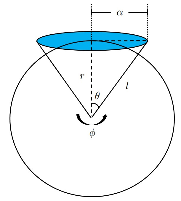
Figure 2: A schematic of a cone embedded into a sphere, illustrating the approximation of a small region of a two-sphere as a flat disk. The relative size of the disk (blue) has been exaggerated for clarity.

Constraining the apex angle of the cone to be small, $\theta\ll 1$, the following relations hold: $\mathrm{tan}\theta=\alpha/r$ (in general) and $\mathrm{tan}\theta\approx\theta$, together giving $\alpha\approx r\theta$. Fixing $r=r_{0}$, one also has $\alpha\approx r_{0}\theta$ and $d\alpha\approx r_{0}d\theta$. The line element describing the base of the cone is then $ds^{2}=d\alpha^{2}+\alpha^{2}d\phi^{2}\approx r_{0}^{2}\left(d\theta^{2}+\theta^{2}d\phi^{2}\right)$, which is precisely (13).

For parameter range $M>0$, this geometry is physically interpreted in the cosmological picture [8] as a spacetime originating in a big bang (the apex of the cylinder), expanding uniformly in the $x$ and $y$ directions (covering the cylinder’s base), and contracting in $z$ (this “fourth” dimension cannot be shown in our schematic); remember that $r$ is timelike in this case, where Figure 2 represents a cosmology. For $M<0$, $r$ is spacelike.

Appendix B: Coordinate transformation to the type D Kasner solution and spaghettification

The coordinate transformation putting Eq. (2) in the form of Eq. (8), i.e. demonstrating that the $M>0$ $AIII$-metric is in fact the type D Kasner vacuum solution, is as follows [8]:

$$t\equiv\left(\frac{3}{4M}\right)^{1/3}z,\qquad r\equiv\left(\frac{9M}{2}\right)^{1/3}\tau^{2/3},\qquad\rho e^{i\phi}\equiv\left(\frac{2}{9M}\right)^{1/3}\left(x+iy\right).$$ (14)

Note that the labelling after the transformation reflects more plainly the nature (timelike or spacelike) of the coordinates.

The specific form of the above coordinate transformation sheds much light on the interpretation of the Kasner metric as a region of the Schwarzschild solution. The radial transformation, i.e. $r\equiv\left(9M/2\right)^{1/3}\tau^{2/3}$, is also precisely the relation between the radial coordinate of an observer falling into a Schwarzschild black hole and the proper countdown time $\tau$ until they reach the singularity $r=0$ [3, 16]. (The observer is assumed to fall inwards with purely radial motion and to begin the fall at a large distance from the black hole.) The countdown time $\tau$ is defined as the proper time at which the singularity will be reached minus the proper time measured by the infalling observer. As the time $\tau$ ticks down in metric (8) (i.e. as $r=0$ is approached), the spacetime can be seen to extend along $z$ and contract circumferentially in $x$ and $y$ at the rate known for an infalling “spaghettified” observer (see p. 862 of Ref. [3]).

The cosmological picture discussed in the main text is in a sense the time-reversal of the deep-radial interpretation, as the big bang and growth of a universe in the cosmological picture is, once the “direction” of coordinate $\tau$ is inverted, the spacetime experienced by an observer falling towards the singularity of a black hole.

Appendix C: Coordinate transformation to the Taub solution

The coordinates of metric (7) can be transformed as [8]

$$t\equiv|M|^{-1/3}\ \tilde{t},\qquad r\equiv 2|M|^{1/3}\ \tilde{z}^{1/2},\qquad\rho e^{i\phi}\equiv\frac{1}{2}|M|^{-1/3}\left(\tilde{x}+i\tilde{y}\right),$$ (15)

yielding

$$ds^{2}=\tilde{z}^{-1/2}\left(-d\tilde{t}^{2}+d\tilde{z}^{2}\right)+\tilde{z}\left(d\tilde{x}^{2}+d\tilde{y}^{2}\right),$$ (16)

the Taub solution, the only plane-symmetric static vacuum solution of Einstein’s field equations.

References

- [1] Stephani, H.; Kramer, D.; MacCallum, M.; Hoenselaers, C.; Herlt, E. Exact Solutions of Einstein’s Field Equations, 2nd ed.; Cambridge University Press: Cambridge, UK, 2003.
- [2] Ehlers, J.; Kundt, W. Exact solutions of the gravitational field equations, in Gravitation: an introduction to current research, ed. Witten, L.; Wiley: London, UK, 1962.
- [3] Misner, C. W.; Thorne, K. S.; Wheeler, J. A. Gravitation; W. H. Freeman and Company: San Francisco, USA, 1973.
- [4] Wald, R. M. General Relativity; University of Chicago Press: Chicago, USA, 1984.
- [5] Carroll, S. M. Spacetime and Geometry; Addison Wesley: San Francisco, USA, 2004.
- [6] Petrov, A. Z. Einstein Spaces; Pergamon Press: Oxford, UK, 1969.
- [7] Belinski, V.; Verdaguer, E. Gravitational Solitons; Cambridge University Press: Cambridge, UK, 2001.
- [8] Griffiths, J. B.; Podolský, J. Exact Space-Times in Einstein’s General Relativity; Cambridge University Press: Cambridge, UK, 2009.
- [9] Bonnor, W. B.; Martins, M. A. P. The interpretation of some static vacuum metrics. Class. Quantum Grav. 1991, 8, 727–738.
- [10] Bonnor, W. B. Physical Interpretation of Vacuum Solutions of Einstein’s Equations. Part I. Time-independent Solutions Gen. Relativ. Gravit. 1992, 24, 551–574.
- [11] Bonnor, W. B.; Griffiths, J. B.; MacCallum, M. A. H. Physical Interpretation of Vacuum Solutions of Einstein’s Equations. Part II. Time-dependent solutions Gen. Relativ. Gravit. 1994, 26, 687–729.
- [12] Zhang, H.; Noh, H.; Zhu, Z. A new class of plane symmetric solution. Phys. Lett. B 2008, 663, 291–296.
- [13] Harvey, A. Will the Real Kasner Metric Please Stand Up. Gen. Relativ. Gravit. 1990, 22, 1433–1445.
- [14] Peres, A. Gravitational field of a tachyon. Phys. Lett. A 1970, 31, 361–362.
- [15] Gleiser, R. J.; Dotti, G. Instability of the negative mass Schwarzschild naked singularity. Class. Quantum Grav. 2006, 23, 5063–5077.
- [16] Lambourne, R. J. A. Relativity, Gravitation and Cosmology; Cambridge University Press: Cambridge, UK, 2010.
- [17] Bedran, M. L.; Calvo, M. O.; Paiva, F. M.; Damio Soares, I. Taub’s plane-symmetric vacuum spacetime reexamined. Phys. Rev. D 1997, 55, 3431–3439.
- [18] Cherubini, C.; Bini, D.; Capozziello, S.; Ruffini, R. Second order scalar invariants of the Riemann tensor: applications to black hole spacetimes. Int. J. Mod. Phys. D. 2002, 11, 827–841.
- [19] Karlhede, A.; Lindström, U.; Åman, J. E. A Note on a Local Effect at the Schwarzschild Sphere Gen. Relativ. Gravit. 1982, 14, 569–571.
- [20] Ong, Y. C. Evolution of Black Holes in Anti-de Sitter Spacetime and the Firewall Controversy; Springer: Heidelberg, Germany, 2016.
- [21] Kasner, E. Geometrical Theorems on Einstein’s Cosmological Equations. Am. J. Math. 1921, 43, 217–221.
- [22] Ellis, G. F. R.; MacCallum, M. A. H. A Class of Homogeneous Cosmological Models. Commun. math. Phys. 1969, 12, 108–141.
- [23] Kasner, E. Solutions of the Einstein Equations Involving Functions of Only One Variable. Trans. Am. Math. Soc. 1925, 27, 155–162.
- [24] Frolov, V. P.; Novikov, I. D. Black Hole Physics: Basic Concepts and New Developments; Kluwer Academic Publishers: Dordrecht, the Netherlands, 1998.
- [25] Frolov, V. P.; Zelnikov, A. Introduction to Black Hole Physics; Oxford University Press: Oxford, UK, 2011.
- [26] Hiscock, W. A.; Larson, S. L.; Anderson, P. R. Semiclassical effects in black hole interiors. Phys. Rev. D 1997, 56, 3571–3581.
- [27] Choptuik, M. W.; Lehner, L.; Pretorius, F. Probing Strong-Field Gravity Through Numerical Simulations, in General Relativity and Gravitation: A Centennial Perspective, eds. Ashtekar, A.; Berger, B. K.; Isenberg, J.; MacCallum, M.; Cambridge University Press: Cambridge, UK, 2015.
- [28] Matyjasek, J. Quantum fields in Bianchi type I spacetimes: The Kasner metric. Phys. Rev. D 2018, 98, 104054.
- [29] Aichelburg, P. C. High Symmetry Fields and the Homogeneous Field in General Relativity. J. Math. Phys. 1970, 11, 1330–1335.
- [30] Taub, A. H. Empty space-times admitting a three-parameter group of motions. Ann. Math. 1951, 53, 472–490.
- [31] Taub, A. H. Plane-symmetric similarity solutions for self-gravitating fluids, in General Relativity: Papers in Honour of J. L. Synge, ed. O’Raifeartaigh, L.; Clarendon Press: Oxford, UK, 1972.
- [32] Horský, J. The gravitational field of planes in general relativity. Czech. J. Phys. B 1968, 18, 569–583.
- [33] Bonnor, W. B. The physical interpretation of a certain static vacuum space-time. Wiss. Z. Friedrich-Schiller-Univ. Jena Nat. wiss. Reihe 1990, 39, 25–29.
- [34] Robinson, I.; Trautman, A. Some spherical gravitational waves in general relativity. Proc. R. Soc. Lond. A. 1962, 265, 463–473.
- [35] Bonnor, W. B. On a Robinson-Trautman solution of Einstein’s equations. Phys. Lett. 1970, 31A, 269.
- [36] Bonnor, W. B. Negative Mass in General Relativity. Gen. Relativ. Gravit. 1989, 21, 1143–1157.
- [37] Miller, B. D. Negative-mass lagging cores of the big bang. Astrophys. J. 1976, 208, 275–285.
- [38] Horský, J.; Novotný, J. On the analogy between the plane and the spherical solutions of Einstein equations in the vacuum. Czech. J. Phys. B 1982, 32, 1321–1324.
- [39] Geroch, R. Limits of Spacetimes. Commun. math. Phys. 1969, 13, 180–193.