Banyan: A Scoped Dataflow Engine for Graph Query Service

Abstract.

Graph query services (GQS) are widely used today to interactively answer graph traversal queries on large-scale graph data. Existing graph query engines focus largely on optimizing the latency of a single query. This ignores significant challenges posed by GQS, including fine-grained control and scheduling during query execution, as well as performance isolation and load balancing in various levels from across user to intra-query. To tackle these control and scheduling challenges, we propose a novel scoped dataflow for modeling graph traversal queries, which explicitly exposes concurrent execution and control of any subquery to the finest granularity. We implemented Banyan, an engine based on the scoped dataflow model for GQS. Banyan focuses on scaling up the performance on a single machine, and provides the ability to easily scale out. Extensive experiments on multiple benchmarks show that Banyan improves performance by up to three orders of magnitude over state-of-the-art graph query engines, while providing performance isolation and load balancing.

1. Introduction

Graph query service (GQS) is widely used in many Internet applications ranging from search engines, recommendation systems, to financial risk management. The global GQS market is estimated to reach $2.9$ billion USD by 2024, with an annual growth rate of $22.2\%$ (GraphDB Annual Growth, [n.d.]). In these applications, data are represented as large-scale graphs such as knowledge graphs and social networks, and the explorations on the data are usually expressed as graph traversal queries. GQS serves these large-scale graphs for interactive query access, allowing many users to submit concurrent graph traversal queries and obtain results in real-time.

Previous graph query engines (Zhao and Han, 2010; Yan et al., 2016; Sakr et al., 2012; Shao et al., 2013; Neo4j, 2021b; Janusgraph, 2021a) mainly focus on optimizing the query latency from the perspective of computation efficiency, i.e., traversing more vertices/edges in a time unit. However, we observe that optimizing for computational efficiency alone is not sufficient to achieve short query latency. A multi-tenant GQS needs to address two key goals to fulfill stringent latency requirements: (O1) fine-grained control and scheduling, as well as (O2) performance isolation and load balancing during the query execution.

	Neo4j	JanusGraph	Timely	GAIA	Banyan
O1-1: Control on Subquery Traversal	✗	✗	✗	✓	✓
O1-2: Subquery-level Scheduling Policy	✗	query-level only	✗	query-level only	✓
O2: Subquery-level Isolation	✗	✗	✗	✗	✓

Table 1. Comparing graph query engines on O1 and O2. TigerGraph (TigerGraph, 2021) is not open-sourced and thus not listed.

Fine-Grained Control and Scheduling (O1). A graph query usually performs many traversals starting from different source vertices in the graph. We observe two key techniques that can reduce query latencies, and in turn boost the system throughput: (O1-1) concurrently executing these traversals, and controlling them at a fine granularity; (O1-2) carefully choosing the traversal strategy.

Example 0 (A Graph Traversal Query in Gremlin).

⬇

g.V(123).repeat(out(‘knows’))

.until(out(‘worksAt’).is(eq(‘XYZ’)))

.or().loops().is(gt(5)))

.where(in(‘tweets’).out(‘hasTag’).is(eq(‘#ABC’)))

.limit(20)

Example 1.1 shows a graph traversal query intended to find 20 users who are within the 5-hop neighborhood of user $123$, work at company ‘XYZ’, and have tweeted with hashtag ‘#ABC’. When executing this query, we need to start a traversal for every user entering the where subquery. This traversal can be canceled immediately if any tweet of the user is found to have the desired hashtag, without needing to check all of that user’s tweets. Clearly, canceling this traversal should not affect the traversals for other users. More importantly, it should not be blocked by other traversals, e.g., by someone who tweets a lot but not with hashtag ‘#ABC’. This implies that a GQS needs to support concurrent execution as well as fine-grained control of subquery traversals (O1-1).

Eagerly checking the hashtags tweeted by one user requires a DFS scheduling policy for the where subquery. The same scheduling policy holds within one loop iteration in the repeat subquery, as we would like to eagerly check if a neighbor works at company ‘XYZ’. However, it would be preferable to use BFS when scheduling across loop iterations of the repeat subquery. This is because we do not want to blindly explore all neighbors within 5 hops if 20 candidates can be found in a much smaller neighborhood. This implies that GQS systems need to support customized traversal policies in subqueries (O1-2).

Performance Isolation and Load Balancing (O2). It is challenging to fulfill the stringent latency requirement in a production environment. Due to the intrinsic skewness in graph data, graph traversal queries can vary dramatically in terms of the amount of computation. Therefore, GQS should be capable of enforcing performance isolation across queries to guarantee the latency SLO. In addition, as illustrated in Example 1.1, for better performance, the isolation granularity needs to be as small as subquery-level traversals. Existing graph databases (Neo4j, 2021b; Neptune, 2021a; Janusgraph, 2021a) map concurrent queries to system threads and rely on the operating system for scheduling. This mechanism does not expose the internal query complexity and thus cannot support subquery-level isolation. The skewness in graph data can lead to dynamic workload skewness at run time, requiring GQS to provide dynamic load balancing.

Table 1 compares existing graph query engines on their supports for O1 and O2. Many graph query engines (Neo4j, 2021a; Mellbin and Åkerlund, 2017; Chen et al., 2019; Qian et al., 2021; Shi et al., 2016; TigerGraph, 2021) use the dataflow model to execute graph traversal queries in languages such as Cypher (Cypher, 2021), Gremlin (Tinkerpop, 2021) and GSQL (TigerGraph, 2021). Existing dataflow models either a) support only static topologies (e.g., Timely (Murray et al., 2013) and GAIA (Qian et al., 2021)) or b) can only dynamically spawn tasks at coarse granularity (e.g., CIEL (Murray et al., 2011)). Specifically, Timely and GAIA attach a metadata (timestamp in Timely and context in GAIA) in every message to identify which subquery traversal it belongs to, but then these systems process messages belonging to different traversals of a subquery in the same static execution pipeline determined at compile time. Without physically isolating the execution of traversals inside a subquery, these systems cannot efficiently support both O1 and O2. Achieving these goals requires flexibly controlling and scheduling the fine-grained subquery traversals spawned dynamically during query execution. We expand more in Section 2 to discuss the limitations of existing dataflow models, and evaluate this issue with experiments in Section 5.

In this paper, we propose a novel scoped dataflow to model graph traversal queries, which supports fine-grained control and scheduling during query execution. The scoped dataflow model introduces a key concept called scope. A scope marks a subgraph in the dataflow, which corresponds to a subquery. The scope can be dynamically replicated at runtime into physically isolated scope instances which correspond to independent traversals of the subquery. Scope instances can be concurrently executed and independently controlled. This way, traversals of a subquery can time-share the CPU and be independently canceled without blocking or affecting each other. Furthermore, a scope allows users to customize the scheduling policy between and inside scope instances, supporting diverse scheduling policies for different parts of a query.

We build the Banyan engine for a multi-tenant GQS, based on an efficient distributed implementation of scoped dataflow. Banyan parallelizes a scoped dataflow into a physical plan of operators, and cooperatively schedules these operators on executors pinned on physical cores. On each executor, Banyan dynamically creates and terminates operators to instantiate and cancel scope instances. Banyan manages operators hierarchically as an operator tree: operators are scheduled recursively by their parent scope operators. This hierarchy allows customized scheduling within each scope, and provides performance isolation both across queries and within a single query. Banyan partitions the graph into fine-grained tablets and distributes tablets across executors. To handle workload skewness, Banyan dynamically migrates tablets along with the operators accessing them between executors for load balancing. In summary, the contributions of this paper include:

1. We propose the scoped dataflow model, which introduces a novel scope construct to a dataflow. The scope explicitly exposes the concurrent execution and control of subgraphs in a dataflow to the finest granularity (Section 3).

2. We build Banyan, an engine for GQS based on a distributed implementation of the scoped dataflow model. Banyan can leverage the many-core parallelism in a modern server, and can easily scale out to a distributed cluster (Section 4).

3. We conduct extensive evaluations of Banyan on popular benchmarks. The results show that Banyan has 1-3 orders of magnitude performance improvement over the state-of-the-art graph query engines and provides performance isolation and load balancing.

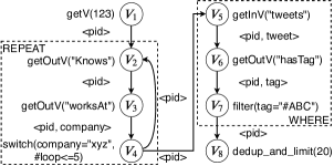
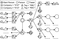
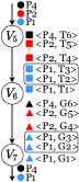
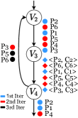
Figure 1. (a) The logical dataflow for Example 1.1. (b) An example data graph. (c)(d) Execution pipelines of the where and repeat subquery of the topo-static dataflow model in Figure 1, respectively. The execution pipelines depict snippets of all messages generated during query execution at the operators.

2. Limitations of Existing Dataflow Models

In the dataflow model, a graph traversal query is represented as a directed graph of operators as vertices, where each operator sends and receives messages along directed edges. Figure 1 presents a typical logical dataflow for Example 1.1, where the repeat subquery is translated into vertices $v_{2}$, $v_{3}$ and $v_{4}$, the where subquery is translated into vertices $v_{5}$, $v_{6}$ and $v_{7}$. Other dataflow models such as Timely (Murray et al., 2013) and GAIA (Qian et al., 2021) share the same main structure demonstrated in Figure 1. A common characteristic of these dataflow models is that their topologies are fixed at compile time. We refer to such dataflow models as topo-static dataflows in the following discussions. Next, we use Example 1.1 on the data graph in Figure 1 to illustrate the limitations of using topo-static dataflows in a GQS.

Control on Concurrent Traversals (O1-1). A graph query usually has subqueries that can launch many independent traversals starting from different vertices in the graph. E.g., each sub-tree rooted at $P_{1}$, $P_{2}$, $P_{4}$ and so on in Figure 1 are independent traversals of the where subquery. Figure 1 demonstrates an example execution pipeline of the where subquery in the topo-static dataflow model in Figure 1, where messages of different traversals (marked in different colors) are mixed in the dataflow and sequentially processed. Although the traversal of $P_{1}$ can be immediately terminated when $V_{7}$ detects $G_{1}$, other messages in the traversal of $P_{1}$ (messages in black rectangles) cannot be trivially canceled: To cancel a specific traversal, one has to annotate each message with extra metadata about which traversal it belongs to, and filter messages by their metadata at operator $V_{5}$-$V_{7}$. GAIA cancels subquery traversals in this way. Alternatively, simply isolating the traversals using different threads will not work. A large number of concurrent traversals can lead to an exploded number of threads, where the context switch overhead will set a hard bottleneck on the system performance. This impact becomes even worse in a multi-tenant environment.

Diverse Scheduling Policies (O1-2). Inside a graph query, different subqueries often have very diverse scheduling preferences. Consider the repeat subquery. Instead of blindly exploring all the 5-hop neighbors, we prefer to gradually expand the exploration radius, as closer neighbors (e.g., $P_{1}$ and $P_{2}$ in the first hop) are more likely to work at the same company with the start person. This corresponds to completing the traversals of earlier iterations first, i.e., in a BFS manner. Meanwhile, inside an iteration we prefer to finish checking if a neighbor is a match before the next, i.e., scheduling operators $V_{2}$-$V_{4}$ in a DFS manner. However, as depicted in Figure 1, in the topo-static dataflow model, messages of different iterations are mixed and may be disordered due to parallel execution, e.g., $P_{4}$ and $P_{5}$ are processed before $P_{1}$ in $V_{3}$. To enforce inter-iteration BFS, one has to annotate each message with its belonging iteration, and sort every incoming message according to this metadata in $V_{2}$-$V_{4}$, incurring much overhead. As far as we know, no existing graph query engine allows configuring subquery-level scheduling policies.

Performance Isolation (O2). In a GQS, the scales of traversals could vary drastically between queries. Even with the same query, different inputs could lead to traversals of very different scales. E.g., on the LDBC benchmark (LDBC Benchmark, 2021), we observed up to three orders of magnitude difference in query latency for the same query with different starting persons. In addition, performance isolation is necessary for concurrent traversals inside subqueries to prevent a traversal with heavy computation from indefinitely blocking other traversals. E.g., in Figure 1 the traversal of $P_{2}$ (messages in red), who tweeted a lot without hashtag #ABC, blocks the traversal of $P_{4}$ (messages in black), even if $P_{4}$ can pass the predicate. This requires the execution framework to provide performance isolation in various granularities, from the level of inter-user in a multi-tenant environment, to the level of inter-traversal within a subquery.

3. Scoped Dataflow

Scoped dataflow is a new computational model that extends the existing dataflow model, with the ability to explicitly expose concurrent execution and control of subgraphs in a dataflow to the finest granularity. In this section, we define the structure of scoped dataflow, introduce the programming model, and demonstrate scoped dataflow can tackle the problems in Sec 2.

3.1. Computation Model

Similar to the traditional dataflow model, a scoped dataflow is also based on a directed graph $G(V,E)$. Vertices in $V$ send and receive messages along directed edges in $E$. The scoped dataflow introduces a new construct named scope. Formally, a scope is a sub-structure of the scoped dataflow $G(V,E)$, and has two system-provided vertices: an ingress vertex and an egress vertex. All the input messages entering a scope pass through its ingress vertex, and all the edges leaving a scope pass through its egress vertex. Inside a scope $S$, vertices which are neither the ingress nor egress of $S$ are referred to as internal vertices of $S$. An internal vertex of $S$ can belong to an inner scope of $S$. If $G(V,E)$ is cyclic, every cycle in $G(V,E)$ must be contained entirely within a scope $S$, and the backward edge must be from a vertex $v$ in $S$, to the ingress vertex of $S$. Since the edges leaving a scope must pass through its egress vertex, $v$ cannot be in any inner scope of $S$. We categorize scopes into two types: a scope without backward edges is called a branch scope, and a scope with backward edges is called a loop scope. Figure 2 shows an example loop scope. Scopes can be well-nested. The nesting level of a scope is called its depth. The depth of a top-level scope is $1$.

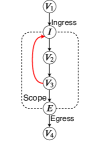
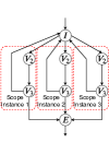
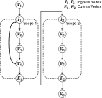
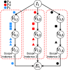
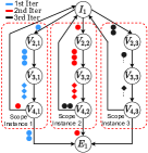
Figure 2. (a) An example loop scope, and (b) an example of its instantiation. (c) The scoped dataflow for Example 1.1, and an instantiation of its (d) branch scope and (e) loop scope.

A scope marks a region inside a dataflow: the dataflow subgraph inside a scope can be dynamically replicated at runtime to create new subgraph instances, isolating the processing of different input data entering the scope. The newly instantiated dataflow subgraph of a scope is called a scope instance. The states of vertices in different scope instances are independent. In a scope $S$, scope instances are instantiated as follows:

• Every inner vertex of $S$ and every edge connecting these inner vertices are copied in the new instance. Note that, the ingress/egress vertices of any inner scopes contained in $S$ are also counted as $S$’s inner vertices. The state of each copied stateful vertex is initialized as the default value.

• Every edge connecting $S$’s ingress/egress vertex and an inner vertex, including backward edges, is copied by replacing the inner vertex with its corresponding copy in the new instance.

Figure 2 shows an example of instantiated scoped dataflow with three scope instances for Figure 2.

For a scoped dataflow $G(V,E)$, we denote its instantiated scoped dataflow as $\tilde{G}(\tilde{V},\tilde{E})$. In $\tilde{G}$, each vertex (resp. edge) in a scope instance can be uniquely identified by the corresponding $v$ (resp. $e$) in $G$, and a scope tag $t$ of the containing scope instance. The scope tag is in the following format:

$$ScopeTag:\langle s_{1},\cdots,s_{d}\rangle\in\mathbb{N}^{d}$$

where an element $s_{k}$ denotes the $s_{k}$-th scope instance in a scope of depth $k$. The vertex (resp. edge) in $\tilde{G}$ identified by $v$ (resp. $e$) and the scope tag $t$ is denoted by $\tilde{v}_{t}$ (resp. $\tilde{e}_{t}$). Vertices and edges not in any scope have an empty scope tag $\langle\rangle$.

Programming Model. In a scoped dataflow, every message bears the scope tag of the edge it passes through. Every vertex implements the following APIs:

$$v.\text{{ReceiveMessage}}(msg:Message,e:Edge,t:ScopeTag)$$

$$v.\text{{OnCompletion}}(t:ScopeTag)$$

A vertex may invoke two system-provided methods in the context of the above callbacks:

$$this.\text{{SendMessage}}(msg:Message,e:Edge,t:ScopeTag)$$

$$this.\text{{NotifyCompletion}}(t:ScopeTag)$$

Users write their logics according to the scoped dataflow $G$, while at runtime the logics are executed by $\tilde{G}$. For instance, $v.$ReceiveMessage(msg, $e$, $t$) defines the logics how $\tilde{v}_{t}$ processes a message received along $\tilde{e}_{t}$. $v.\text{{OnCompletion}}(t)$ defines the logics executed when vertex $\tilde{v}_{t}$ has no more input, e.g., an aggregate operator emits the final aggregation results when it sees all the inputs. $\text{{SendMessage}}(msg,e,t)$ sends a message along with edge $\tilde{e}_{t}$. $\text{{NotifyCompletion}}(t)$ can be called if an operator would like to terminate processing proactively, e.g., a limit operator terminates once it generates enough outputs.

Scope Instantiation. In a scope, the ingress vertex instantiates scope instances and routes the messages entering this scope to different scope instances. The egress vertex manages the termination of scope instances inside a scope. Scope instances can be terminated independently of each other. The ingress and egress vertices only act on the scope tags of messages passing through. In specific, for each message $msg$ passing through:

• The ingress vertex routes $msg$ to a destination scope instance $SI$ and sets the scope tag of $msg$ to that of $SI$. If $SI$ does not exist, the ingress vertex instantiates it.

• The egress vertex removes the last element in the scope tag of $msg$. When OnCompletion($t$) is called in the egress, it terminates the scope instance with scope tag $t$.

Branch and loop scopes have different behaviors on how messages are mapped to scope instances. In a branch scope, every input message triggers the instantiation of a new scope instance. Whereas in a loop scope, messages from edges entering the scope with scope tag $\langle s_{1},\cdots,s_{d}\rangle$ are routed to the scope instance with scope tag $\langle s_{1},\cdots,s_{d},1\rangle$; messages from backward edges with scope tag $\langle s_{1},\cdots,s_{d},s_{d+1}\rangle$ are routed to scope instance with scope tag $\langle s_{1},\cdots,s_{d},s_{d+1}+1\rangle$. A configurable threshold, Max_SI, can be set to constrain the maximal number of concurrent scope instances in a scope.

Scope Scheduling. Scoped dataflow supports customizing scheduling policies for scopes. The scheduling policy of a scope can be decoupled into two parts: inter-scope-instances (inter-SI) policy and intra-scope-instance (intra-SI) policy. The inter-SI policy specifies the scheduling priorities of scope instances inside a scope. The intra-SI policy specifies the scheduling priorities of inner vertices (an inner scope as a whole is treated as a virtual inner vertex) inside a scope instance. Users can customize the scheduling policies with the below comparators:

$$bool~{}\text{{InterSI\_Comparator}}(t_{1}:ScopeTag,t_{2}:ScopeTag)$$

$$bool~{}\text{{IntraSI\_Comparator}}(v_{1}:VertexID,v_{2}:VertexID)$$

The inter-SI comparator decides the priorities of scope instances. The intra-SI comparator decides the priorities of inner vertices in the same scope in $G(V,E)$.

For any two vertices $\tilde{u_{t_{1}}}$ and $\tilde{v_{t_{2}}}$ in $\tilde{G}$, their scheduling orders are decided iteratively according to the following rules. Without loss of generality, we denote the depths of $t_{1}$ and $t_{2}$ as $d_{1}$ and $d_{2}$, and assume $d_{1}\leq d_{2}$. We use $anc_{d}(\tilde{v_{t}})$ to denote the ancestor scope instance of $\tilde{v_{t}}$ at depth $d$.

• We start comparing the ancestor scope instances of $\tilde{u_{t_{1}}}$ and $\tilde{v_{t_{2}}}$ from depth $1$ to depth $d_{1}$.

• At depth $d$, if $anc_{d}(\tilde{u_{t_{1}}})$ and $anc_{d}(\tilde{v_{t_{2}}})$ are the same, we proceed to depth $d+1$.

• At depth $d$, if $anc_{d}(\tilde{u_{t_{1}}})$ and $anc_{d}(\tilde{v_{t_{2}}})$ are different scope instances of the same scope $S$, the priority is determined by calling the inter-SI comparator of $S$ on the scope tags of $anc_{d}(\tilde{u_{t_{1}}})$ and $anc_{d}(\tilde{v_{t_{2}}})$.

• At depth $d$, if $anc_{d}(\tilde{u_{t_{1}}})$ and $anc_{d}(\tilde{v_{t_{2}}})$ belong to different scopes in a common parent scope $S$, the priority is determined by calling the intra-SI comparator of $S$ on the scopes of $anc_{d}(\tilde{u_{t_{1}}})$ and $anc_{d}(\tilde{v_{t_{2}}})$.

3.2. Progress Tracking

To correctly invoke $\text{{OnCompletion}}(t)$ for vertices, a scoped dataflow needs to track the processing progress of its vertices, i.e., when a vertex is guaranteed to have received all its inputs. The scoped dataflow model adopts an EOS-based progress tracking mechanism similar to the Chandy-Lamport algorithm (Chandy and Lamport, 1985). After ingesting all the external inputs, the runtime automatically inserts an EOS message to the dataflow. EOS messages are propagated through the dataflow graph to facilitate the progress tracking. Once a vertex receives EOS messages from all its incoming edges, it calls $\text{{OnCompletion}}(t)$, and then emits an EOS message in all its outgoing edges.

However, as a scoped dataflow can dynamically instantiate scope instances and may contain cycles, we extend the aforementioned EOS-based progress tracking mechanism in order to support the scoped dataflow.

Hierarchical Progress Tracking. We track progress hierarchically in a scoped dataflow, i.e., progress tracking inside and outside a scope are conducted separately. Progress tracking outside a scope $S$ simply treats $S$ as a virtual vertex, denoted $v_{S}$. The runtime conducts progress tracking on the dataflow subgraph inside a scope $S$ to decide the completion of $v_{S}$, which completes when the ingress vertex of $S$ receives EOS from all its input edges, and all the scope instances inside $S$ have completed. Once $v_{S}$ reaches completion, the egress vertex of $S$ emits EOS along all its outgoing edges.

Tracking inside a Scope. Next, we explain how the progress tracking is done inside the branch and loop scope, respectively.

In a branch scope, the runtime propagates EOS in each scope instance to track their progress independently. An ingress vertex reaches completion when it has received EOS from all its incoming edges. After completion, the ingress vertex sends the largest scope instance ID it has spawned to the egress vertex of the same scope. The egress decides the number of scope instances according to this ID. When the egress vertex has tracked that all the scope instances in this scope have completed, it reaches completion and emits EOS to the outgoing edges.

Progress tracking of loop scopes is extended from that of the branch scopes. To decide when the loop iteration reaches completion, the ingress vertex tracks the scope tags of data and EOS messages received from the backward edges. If an ingress vertex only receives EOS but no data messages for a specific scope instance, the ingress vertex can infer that this scope instance is the last loop iteration. This way, the ingress vertex can infer the number of spawned scope instances. With this information, the egress vertex tracks the progress of scope instances in the same way as the branch scope. This process is guaranteed to be able to stop due to the simple fact that if you remove the ingress vertex inside a loop scope (note that the ingress vertex only forwards messages) and directly connect the edges according to the forwarding behavior of the ingress vertex, the instantiated scope dataflow is a DAG without cycles.

3.3. Scoped Dataflow in Action

In this section, we discuss the applicability of scopes, followed by an example explaining how the scoped dataflow model can be used to solve the challenges discussed in Section 2.

Applicability of Scopes. The scoped dataflow model is designed to facilitate fine-grained control on subquery traversals and enforce scope-level customization of scheduling policies. In general, scopes can benefit graph queries with:

• Where subqueries which can be early canceled. As the instantiation of scope instance brings overhead (see E2 in Section 5.3). For where subqueries which cannot be early canceled, scopes should be turned off.

• Loop subqueries that can find matches more quickly following certain exploration strategy (e.g., BFS or DFS).

Note that, the benefit of scope is query/data-dependent (see E2 in Section 5.3). The best plan should be determined by the query compiler, which is beyond the scope of this paper.

Example 0 (Implementation of vertex $V_{7}$ in Figure 2).

⬇

class V7Filter:Vertex {

void ReceiveMessage(msg:Message, e:Edge, t:ScopeTag) {

if (msg.GetTag() == "#ABC") {

SendMessage(msg.getPersonId(), out_e, t);

NotifyCompletion(t);}

}

void OnCompletion(t:Tag) { }

}

Example 0 (Implementations of the inter-SI BFS and intra-SI DFS policies).

⬇

bool InterSI_BFS:InterSI_Comparator(t_1:ScopeTag, t_2:ScopeTag) {

return LexicalOrderCompare(t_1, t_2);

}

bool IntraSI_DFS:IntraSI_Comparator(v_1:VertexID, v_2:VertexID) {

return v_1 < v_2;

}

Examples of Scopes. Figure 2 shows the scoped dataflow for Example 1.1. Figure 2 zooms in the where subquery of Figure 2, and demonstrates instantiations of scope $2$. Traversals triggered by different users entering the where subquery are mapped to different scope instances, which can be executed concurrently and controlled independently. This way, a user (e.g., the blue one) who posts many tweets without the specified tag will not block the exploration of other users (e.g., the red and black ones) entering the where subquery.

Example 3.1 shows the implementation of the filter vertex $v_{7}$ in Figure 2, which enables early cancellation: On receiving a message $msg$, if the tag in $msg$ is a match, the vertex notifies the completion of itself by calling $\text{{NotifyCompletion}}(t)$ to trigger its cancellation. As a scope instance can be terminated independently, when a match (the red message marked in black box entering $v_{7,2}$) is found, the corresponding scope instance ($v_{5,2},v_{6,2},v_{7,2}$) can be canceled without impacting the other scope instances.

The scheduling policies of scopes can be flexibly configured to fulfill the diverse scheduling preferences of different parts in a graph query. Figure 2 shows that iterations of the repeat subquery in Figure 2 are mapped into different scope instances of the loop scope. We configure a BFS inter-SI scheduling policy such that the blue scope instance (the first iteration) is executed first, then the red one (the second iteration), and the black one (the third iteration) as the last. Meanwhile, by enforcing a DFS intra-SI policy, vertices inside the blue scope instance are scheduled in the order of $\tilde{v}_{4,1}$, $\tilde{v}_{3,1}$ and $\tilde{v}_{2,1}$. Implementations of the inter-SI BFS and intra-SI DFS policy are presented in Example 3.2.

4. Building Banyan on Scoped Dataflow

We build Banyan, an engine for GQS based on a distributed implementation of the scoped dataflow model. Banyan is designed to efficiently leverage the many-core parallelism in a modern server, and agilely balance the workloads across cores. Banyan can also easily scale out to a distributed cluster.

The overall system architecture of Banyan is presented in Figure 3. A Banyan cluster consists of a group of worker nodes, each of which manages multiple executors. An executor exclusively runs in a system thread pinned in a physical core, and is in charge of a partition of the graph data. Vertices in a scoped dataflow are parallelized into operators, and are mapped to executors. Executors communicate with each other through message queues inside the worker node and through TCP connections across worker nodes. In a worker node, executors schedule their own operators and are scheduled by the worker scheduler. The worker scheduler is responsible for balancing the workloads across executors in a worker node.

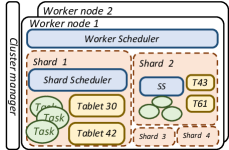
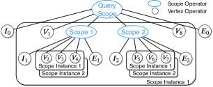
Figure 3. (a) The system architecture of Banyan. (b) An operator tree mapped from the dataflow in Figure 2 in an executor.

4.1. Parallelizing A Scoped Dataflow

Banyan parallelizes a dataflow $G$ into a physical plan of operators in a data-parallel manner. Every vertex in $G$ is parallelized into a set of operators, each encapsulating the processing logic of this vertex. Each edge in $G$ has a partitioning function controlling the data exchange between the operators. In the physical plan, the vertices in $G$ are replaced with the corresponding set of operators, and the edges in $G$ are replaced with a set of edges connecting these operators. At runtime, when we instantiate a scope in $G$ into scoped instances, every scope instance inherits the physical plan of the scope. That is, every scope instance has a complete copy of the corresponding operators and edges of its scope.

Banyan partitions the graph into tablets distributed across executors. A tablet contains an exclusive set of graph vertices and all their in/out edges, along with their properties. We refer to vertices in $G$ that need to access graph data as graph-accessing vertices. To exploit data locality, a graph-accessing vertex is parallelized into as many operators as the number of tablets, and are mapped to the executors hosting the tablets.

This mechanism fits well with the NUMA architecture. As graph-accessing operations are often highly random, by collocating each graph-accessing operator and the corresponding tablet in one executor, we can utilize the low-latency intra-node random memory access in NUMA servers (Zhang et al., 2015). Messages passing across executors are batched to utilize the high bandwidth of sequential memory access across NUMA nodes.

4.2. Executor Internals

In Banyan, executors are single-threaded and each one is pinned in a physical core. Executors schedule their operators cooperatively, allowing Banyan to concurrently process a large number of operators without facing the bottleneck caused by context switch. Cooperative scheduling is based on an asynchronous task-based programming interface. E.g., an operator blocked by an asynchronous I/O operation automatically yields CPU, and the corresponding executor schedules another operator ready for execution. This way, Banyan can overlap CPU computation with networking and I/O, and thus improve the resource utilization.

Scope Operator. The key difference between the scoped dataflow and the traditional dataflow is the introduction of the scope abstraction. To facilitate the scope-based scheduling in Banyan (see Section 3.1), we deliberately introduce scope operators to manage the creation, termination and scheduling for all the operators of a scope. In specific, on every executor containing operators of a scope $S$, we create a scope operator managing all the local operators of $S$ in this executor. The scope operator of $S$ is also managed by the scope operator of $S$’s parent scope (if existed). Therefore, all the operators in an executor can be managed as a forest of operator trees. In each tree, the leaf nodes are operators of vertices and the non-leaf nodes are the scope operators. The operators in an executor are scheduled hierarchically: (1) The executor schedules the root scope operators of queries. (2) When a scope operator of scope $S$ is scheduled, it further schedules its child (scope) operators following $S$’s inter-SI and intra-SI scheduling policies.

Banyan enforces the performance isolation guarantee in each single executor. We take scope operator as the basic unit of resource allocation: resources allocated to scopes operators at the same depth are isolated, and an operator can only consume the resources allocated to its parent scope operator. Once being scheduled, an operator is assigned a quota CPU time by its parent, which constrains the maximum amount of CPU time this operator can use at this round of scheduling, and yields immediately after using up its quota. The vertex operator updates its quota after processing a message, and thus will not occupy an executor for a long time.

By modeling different queries or tenants as the top-level scopes, Banyan can naturally support performance isolation across queries or users. Figure 3 shows the operator tree mapped from the scoped dataflow in Figure 2.

4.3. Hierarchical Operator Management

In this subsection, we introduce how operators are addressed, created and terminated in Banyan.

Operator Addressing. In Banyan, each operator has a unique address, encoding the path from the executor to this operator in the operator tree. The address consists of three parts:

$$\left\langle exec\_id,~{}~{}~{}~{}(sop\_id_{1},s_{1}),\cdots,(sop\_id_{d},s_{d}),~{}~{}~{}~{}op\_id\right\rangle$$

where $exec\_id$ identifies the hosting executor of the operator; $op\_id$ represents the ID of the operator; $(sop\_id_{1},s_{1}),\cdots,(sop\_id_{d},s_{d})$ denotes the chain of ancestor scope operators ($sop\_id_{k}$) and the corresponding scope instance IDs ($s_{k}$). Actually, $\langle s_{1},\cdots,s_{d}\rangle$ is the scope tag of the operator.

To facilitate hierarchical scheduling, each scope operator maintains a directory of its child operators as a prefix tree, using the addresses of child operators as the keys and the pointers to these operators as the values. In the prefix tree, the operators of a scope instance are naturally grouped together as they share the same prefix in their addresses, and thus can be quickly located.

Operator Creation and Termination. Banyan is event-driven, it dynamically creates operators on request. More specifically, sending a message to a non-existing operator triggers the creation of this operator and all its non-existing ancestor scope operators. A scope operator provides a system-level API TerminateScope(scope_instance_id) to terminate a scope instance, i.e., all the operators in this scope instance. Terminating a scope operator will terminate all managed scope instances in cascade. Messages sent to terminated operators are ignored. Banyan recycles objects used for operators through memory management to avoid excessive memory allocations.

4.4. Parallelizing Progress Tracking

In the mechanism of hierarchical progress tracking in Section 3.2, tracking inside a scope requires the ingress vertex to notify the egress vertex of the total number of instantiated scope instances. When the ingress and egress vertices of a scope are parallelized, a single ingress operator may not be aware of all the scope instances in this scope.

To tackle this problem, in a branch scope, each ingress operator broadcasts to all the egress operators the largest ID of scope instances it has instantiated, and each egress operator takes the maximum among these IDs as the total number of scope instances to be tracked. In the case of loop scopes, every time an ingress operator only sees the EOS messages but no data message from a specific loop iteration, it broadcasts to all the egress operators the ID of the corresponding scope instance. If an egress operator receives a specific scope instance ID from all the ingress instances, it can conclude that this ID is the number of scope instances in this scope.

To reduce the number of operators created for a scoped dataflow, Banyan skips creating operators that only receive EOS messages in their entire lifetime. Instead, it handles EOS messages sent to these operators in their parent scope operator. EOS messages sent to non-existing operators are buffered in their parent scope operator. If the operator is created later, these buffered EOS messages are inserted into their mailboxes. Otherwise, the parent scope operator emits EOS messages on behalf of the non-existing child operator after receiving all the corresponding EOS messages.

4.5. Load Balancing

Many realistic graphs are often scale-free, which may lead to a skewed workload distribution among different tablets. And this skewness changes dynamically, as the graph accessing patterns of the incoming queries continuously change. In graph queries, graph-accessing operations are often the most costly part during the execution. To facilitate load balancing between executors, we deliberately partition the graph into more tablets, and migrate tablets together with their graph-accessing operators across executors. Upon migrating a tablet between hosts, we do not migrate the operators at execution (as graph traversal queries are usually short-lived), but only redirect the incoming queries.

5. Evaluations

In this section, we evaluate the performance of Banyan in the following aspects:

• (E1) We study the overall performance of Banyan by comparing single-query latency with state-of-the-art graph query engines (Section 5.2).

• (E2) We study the effects and overheads of scopes on query performance, by comparing the scoped dataflow with the Timely dataflow model (Section 5.3).

• (E3) We study how well Banyan can scale up in a many-core server and scale out in a distributed cluster (Section 5.4).

• (E4) We study how well Banyan can enforce performance isolation and load balancing (Section 5.5).

5.1. Experiment Setup

Benchmarks. We use two benchmarks in the experiments: the LDBC Social Network Benchmark (Angles et al., 2020; LDBC Benchmark, 2021) and the Complex Query(CQ) benchmark.

LDBC is a popular benchmark of graph traversal queries. We selected $12$ queries ($IC_{1}$ - $IC_{12}$) from the $14$ Interactive Complex Read queries in the LDBC benchmark, and exclude all the Analysis ($BI_{1}$-$BI_{25}$), Short Read ($IS_{1}$-$IS_{7}$), and Update queries ($IU_{1}$-$IU_{8}$). $IC_{13}$ and $IC_{14}$ are excluded as they both have shortest-path subqueries, which are typical graph analytics queries. We use two LDBC datasets with scale factor $1$ and $100$, denoted as LDBC-1 and LDBC-100. Table 2 shows the statistics of these two datasets. For each query on both datasets we use the LDBC generator to generate $50$ parameters.

Dataset	# Vertices	# Edges	CSV Size
LDBC-1	$3,181,364$	$17,299,165$	$882$M
LDBC-100	$282,637,871$	$1,777,459,239$	$88$G

Table 2. Dataset Statistics

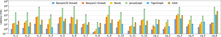
Figure 4. (a) The single-query performance of Banyan, Neo4j, JanusGraph, TigerGraph and GAIA on a single machine with 32 cores. (b) The single-query performance of Banyan, TigerGraph and GAIA in a 4-node cluster (each node has 8 cores).

Real-world service scenarios (e.g. search engines) often select the top-k results from a limited size of recalled candidates to guarantee interactive response. This is different from the query patterns in LDBC (all LDBC queries require sorting the entire results). To better study the effects of scopes, we compose the CQ benchmark with $6$ queries ($CQ_{1}$ - $CQ_{6}$) by adjusting the LDBC queries (e.g., removing the sort operator) based on the two LDBC datasets. Each CQ query has $10$ parameters generated by the LDBC benchmark for both datasets. The CQ queries are presented in Appendix A.

System Configurations. All the experiments are conducted on a cluster (up to $8$ machines) where each machine has $755$G memory and $2$ Intel Xeon Platinum 8269CY CPUs (each with $26$ physical cores and $52$ hyper-threads).

We choose four baseline systems from the most popular or latest graph databases/engines: two single-machine ones—Neo4j $4.1.1$ (Neo4j, 2021b) and JanusGraph $0.5.0$ (Janusgraph, 2021a), as well as two distributed ones—TigerGraph $3.1.0$ (TigerGraph, 2021) and GAIA (Qian et al., 2021). We also compare scoped dataflow with Timely dataflow (Murray et al., 2013) to study the effects of scopes on query performance. For a fair comparison, we implement queries in the Timely dataflow model using Banyan with scopes turned off.

Unless explicitly explained, all the experiments are conducted in a container which has $32$ cores and $700$G memory. We configure a cache size (if available) large enough to store the entire datasets. We build the same set of indexes for all systems, i.e., a primary index on vertex ID for each type of vertices. In graph databases, we execute queries without transactions or as read-only transactions to minimize the transaction overhead. Configurations of the baseline systems are as follows:

• Neo4j 4.1.1. We use $32$ worker threads and turn on query cache.

• JanusGraph 0.5.0. We use BerkeleyJE $7.5.11$ (Oracle Berkeley DB, 2017) as the storage.

• TigerGraph 3.1.0. The distributed query mode is used in the distributed experiments. TigerGraph requires installing a query before execution, and the installation takes much more time (more than $1$ min on average) than query execution. We exclude the installation time in the reported results.

• GAIA. GAIA is only experimented on a subset of the LDBC and CQ queries, as it does not support $IC_{4}$, $IC_{10}$, $CQ_{2}$, $CQ_{4}$ and $CQ_{5}$ . The number of workers is set to $32$ such that GAIA can use all the cores.

• Banyan. We use a C++ version of the backend storage used by JanusGraph (BerkeleyDB $18.1.32$ (Oracle Berkeley DB, 2021)), and directly import the databases exported from JanusGraph. For each dataset, Banyan randomly partitions the graph into $64$ tablets. We rely on the load balancing mechanism to uniformly distribute tablets on executors. We apply loop scope on all the repeat subqueries and branch scope on where subqueries whose branches can be early canceled. Unless otherwise specified, we use $32$ executors for query execution.

Experiment Methodology. To flexibly control query submission, we extend the standard LDBC client to allow specifying the number of concurrent queries ($W$) a client can submit. Unless explicitly specified in E3 and E4, we use $W=1$ throughout the experiments. As LDBC/CQ queries are templates, unless otherwise specified, we follow the LDBC benchmark convention and for each query report the average latency of all the generated parameters. Throughout this section, for each data point we run the corresponding experiment $10$ times to warm up the system, and collect the results from the following $10$ runs. We report the minimum, maximum, and average values of the $10$ results in the figures. Queries run longer than $60$ seconds are marked as timeout.

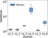
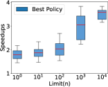
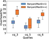
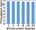
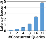
Figure 5. (a) The per-parameter latency speedups of scoped dataflow compared to Timely. (b) The per-parameter latency speedups of the best-case scheduling policy compared to the FIFO policy. (c) The overheads of scope instantiation when MAX_SI is set to 1 and unlimited. The (d) throughput and (e) latency of Banyan under different numbers of concurrent queries.

5.2. Overall System Performance

In this section, we study the performance of Banyan by comparing its single-query latencies on both the LDBC and CQ benchmarks with baseline systems.

Single-machine. In this experiment, we use the LDBC-1 dataset so that baselines like JanusGraph can finish most queries before timeout. The results are depicted in Figure 4.

On the LDBC queries, Banyan has $5$X to three orders of magnitude latency improvement over all the baseline systems except for TigerGraph. Banyan outperforms TigerGraph by up to $14$X for $10$ out of the $12$ LDBC queries (including all the large queries), and is slightly slower on $IC_{3}$ and $IC_{6}$ (both are small queries). As TigerGraph is not open-sourced, we cannot analyze how the query installation helps in speeding up query execution. This demonstrates that Banyan can well utilize the many-core parallelism.

On the CQ queries which can benefit more from the scoped dataflow, the advantage of Banyan further widens, e.g., up to $130$X and $726$X faster than TigerGraph and GAIA, respectively. This improvement is led by the fine-grained control and scheduling enabled by scoped dataflow: (1) subquery traversals (where subqueries in $CQ_{3}$, $CQ_{4}$, $CQ_{5}$ and $CQ_{6}$) can be early canceled, and (2) customized scope-level scheduling policies (e.g., DFS in the loop of $CQ_{1}$ and BFS in the loop of $CQ_{2}$) can trigger the (sub-)query cancellation earlier. Note that GAIA’s support for traversal-level early cancellation is less efficient. GAIA mixes messages with different ‘contexts’ in the same execution pipeline. Canceling a specific traversal requires filtering all messages with the corresponding context at each operator inside a scope. This inefficiency is especially reflected by the performance of GAIA on $CQ_{1}$ and $CQ_{6}$. Differently, Banyan can directly drop scope instances along with all related messages. Besides, GAIA cannot configure scope-level scheduling policies, which influences its performance on $CQ_{3}$ and $CQ_{6}$.

Note that JanusGraph and Neo4j cannot parallelize queries whose traversal starts from a single vertex. To make a fair comparison, we also present the single-thread performance of Banyan, which outperforms both systems on all queries.

Distributed. For the distributed experiment, we use the LDBC-100 dataset and a cluster of $4$ worker nodes each hosting a container of $8$ cores. We compare only the distributed baseline systems. The results are presented in Figure 4. Banyan outperforms TigerGraph by $5$X to $40$X on the LDBC benchmark, and $2$X to three orders of magnitude on the CQ benchmark. These results are consistent with the single-machine experiment, as the benefits of efficiently utilizing hardware parallelism and the scoped dataflow are still tenable in the distributed environment. Banyan is faster than GAIA on most of the LDBC queries and all the CQ queries, except for three small queries ($IC_{2}$, $IC_{7}$ and $IC_{8}$). This is because the graph partitioning in Banyan can incur some overhead due to message passing between executors.

5.3. Benchmark on Scoped Dataflow

In this section, we use the CQ benchmark on the LDBC-100 dataset to study: (1) the effects of scoped dataflow, (2) the effects of scheduling policy and (3) the overhead of scope instantiation. We run each query with ten different parameters, compute the speedup(overhead) between different competitors on each parameter, and report the boxplot of all the per-parameter speedups(overheads) for each query.

Effects of Scoped Dataflow. We report the boxplots of speedups brought by scopes by comparing scoped dataflow against Timely in Figure 5. Note that, the Timely versions of queries are implemented using Banyan with scopes turned off to make a fair comparison. We can see the effects of scoped dataflow are:

• Query-dependent. E.g., the scoped dataflow brings $1.3$X to $36$X latency improvement compared to Timely on average. In particular, the speedup of scoped dataflow on $CQ_{1}$ is relatively small, as $CQ_{1}$ has no subquery which can be early canceled, and the speedup comes from customizing the scope-level scheduling policy, i.e., using DFS to prioritize the loop iteration which generates the final outputs. On the other hand, as $CQ_{4}$ contains a where subquery nested with a loop subquery, canceling a where traversal can save a huge amount of computation.

• Data-dependent. The speedup of scoped dataflow varies on different parameters, e.g., $14$X to $86$X on $CQ_{4}$. This is because different traversals of the where subquery in $CQ_{4}$ have very different computation cost.

Clearly, the optimal scoped dataflow plan should be determined by a query compiler according to the query structure and data statistics.

Effects of Scheduling Policy. In this experiment, we select $CQ_{6}$ (see Appendix  A) and compare the latency of $CQ_{6}$ in Banyan between two cases: (1) the best-policy case where the intra-SI policy of the query and the where subquery are both set to DFS, and (2) the FIFO case where all the scheduling policies are set to FIFO in the query. We also vary $n$ in $CQ_{6}$’s limit(n) clause from $1$ to $10^{4}$. Figure 5 shows the boxplots of speedups brought by best-policy over FIFO. We can see that best-policy outperforms FIFO in all the settings. By increasing the value of $n$ from $1$ to $10^{4}$, the speedups of best-policy widen from $1.8$X to $3.5$X. This is because FIFO can result in more wasted traversals which have no contribution to the final outputs, and this wastage becomes worse with the increasing number of total traversals. Similar effects can be observed in other CQ queries and thus omitted. This experiment shows that customized scheduling policy is necessary for graph queries.

Overhead of Scope Instantiation. To quantify the overhead of scope instantiation, we turn off early cancellation in Banyan, use purely FIFO for scheduling, and compare its single query latencies with Timely. We experiment on $CQ_{3}$, $CQ_{5}$ and $CQ_{6}$, as these queries contains where subqueries that can instantiate a large number of scope instances. We remove the limit clause in these queries to make sure that both Banyan and Timely perform the same amount of traversals. We report the boxplots of overheads caused by scope instantiation in Figure 5.

We can see that without limiting MAX_SI, Banyan is on average $25\%$ slower than Timely, as Banyan suffers from extra scheduling overheads among SIs and a high memory pressure in this case. While, setting MAX_SI in Banyan to $1$ shrinks the performance differences to $13\%$. Note that, MAX_SI is an executor-local configuration. With $32$ executors running in parallel, setting MAX_SI to $1$ allows Banyan to instantiate at most $32$ concurrent SIs of a scope, which is enough to saturate the multi-core parallelism. This experiment shows that the overhead of scope instantiation is limited compared with the benefits of scopes as shown in the first experiment of E2.

5.4. Scalability of Banyan

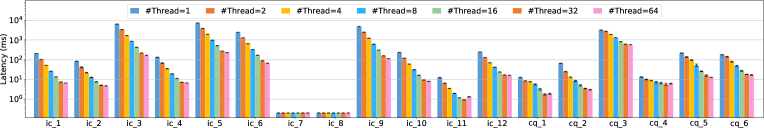
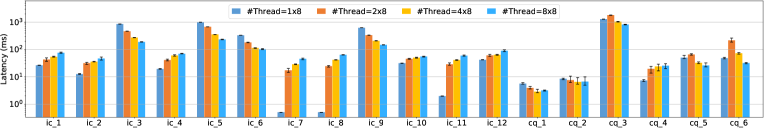
Figure 6. (a) The scale-up performance of Banyan with increasing number of executors on a single machine. (b) The scale-out performance of Banyan with increasing number of worker nodes in the cluster.

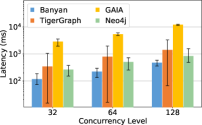
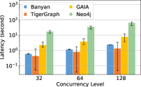
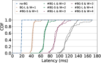
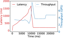
Figure 7. The latency of Banyan, TigerGraph, GAIA and Neo4j under different concurrent workloads: (a) the latency of small queries and (b) the latency of large queries. (c) The latency CDF of the foreground query under different background workloads. (d) The throughput and latency of Banyan before and after load balancing.

Next we conduct experiments to evaluate the scalability of Banyan from three perspectives: (1) the scale-up performance on a many-core machine, (2) the scale-out performance in a cluster, and (3) the throughput and latency when scaling the number of concurrent queries. We use both the CQ and LDBC benchmarks with the LDBC-100 dataset in this experiment.

Scale-Up. In this experiment, we use a single container and vary the number of cores from $1$ to $64$. We report the query latency of Banyan in Figure 6. We can see that the query latency scales almost linearly up to $32$ cores. This is because the architecture of Banyan can efficiently parallelize a query dataflow into fine-grained operators and evenly distribute them across executors. The performance improvement of Banyan stagnates when scaling up from 32 cores to 64. This is because per-executor workload becomes too small to fully utilize allocated computation resources. On the other hand, the hyper-threading has a negative impact on the cache locality when the $64$ logical cores share $52$ physical cores.

Scale-Out. In Figure 6, we study the scale-out performance of Banyan. We use a container of $8$ cores as the worker node, and increase the number of worker nodes from $1$ to $8$. We can observe that by increasing the number of worker nodes, the latencies of large queries (e.g., $IC_{3}$, $IC_{5}$, $IC_{6}$ and $IC_{9}$) decrease in a nearly linear manner. This shows that the scoped dataflow can be well parallelized in a distributed environment, saturating the hardware parallelism. For small queries (e.g., $IC_{1}$, $IC_{2}$, $IC_{10}$, $IC_{11}$ and $CQ_{4}$) with limited computation to distribute, increasing the number of worker nodes results in slightly worse query latency due to the network communication cost. Note that we randomly partition the graph data in Banyan, which is not optimized to reduce inter-machine communication. As graph partitioning is orthogonal to our work, we believe adopting advanced graph partitioning (Hendrickson and Kolda, 2000) can further improve the scale-out performance of Banyan.

Scalability with Concurrent Queries. In this experiment, we use $IC_{6}$ with a fixed parameter to isolate the latency difference caused by different queries and parameters. We vary the submission concurrency $W$ of the client from $1$ to $32$, and report the throughput and latency of Banyan in Figure 5 and 5. As shown in Figure 5, by increasing the number of concurrent queries, Banyan can provide a stable throughput (less than 2% throughput decrease when $W=32$). The query latency is increasing linearly with more concurrent queries executing in the system (Figure 5), which clearly shows that Banyan can fairly time slice the CPU time among concurrent queries, but incur little overhead when running more queries at the same time. We can observe similar results on other queries.

5.5. Performance Isolation & Load Balancing

In this subsection, we study whether Banyan can enforce performance isolation and load balancing. In the following experiments we use a fixed parameter for each selected query as the effects of performance isolation and load balancing are query/parameter-independent.

Performance Isolation. We conduct two experiments to study performance isolation in Banyan.

In the first experiment, we compare the performance isolation in Banyan, Neo4j, TigerGraph and GAIA using the LDBC benchmark with dataset LDBC-1. In Figure 7 and 7 we simulate a mixed workload of large queries (using $IC_{9}$) and small queries (using $IC_{1}$), and vary the submission concurrency $W$ from $32$ to $128$.

For different $W$, Banyan provides on average $2$X-$23$X better query latencies for small queries compared with all the baselines (Figure 7), and $3$X-$30$X performance boost on large queries compared with GAIA and Neo4j (Figure 7). TigerGraph runs $50\%$ faster than $Banyan{}$ on the large queries, but sacrifices its performance on small queries (on average $3.3$X worse than Banyan). Banyan also achieves a much more stable latency performance than TigerGraph. In Figure 7, when $W$ is set to $128$, the latency of TigerGraph fluctuates on small queries at a range of nearly $3000$ms ($2$X of its average). In comparison, the latency of Banyan only fluctuates within $50$ms ($10\%$ of its average). This shows that the hierarchical scheduling in scoped dataflow can guarantee performance isolation between queries.

In the second experiment, we conduct a controlled experiment on how background workload impacts a foreground query. We generate a background workload of different types of queries using the LDBC-100 dataset, i.e., of purely large queries ($IC_{9}$) or purely small queries($IC_{10}$), and vary the concurrency $W$ from $1$ to $4$. While the background queries are executing, we submit a small foreground query ($IC_{1}$) and collect its latency using another client with $W=1$. For each background configuration, we submit the foreground query for $100$ times and plot the CDF of the query latency in Figure 7. We also plot the foreground latency without any background workload (No-BG) as a baseline reference. We can see that when $W$ is fixed, the latency of the foreground query is quite stable. Changing the background workload from small queries (BG-S) to large queries (BG-L) has negligible impact on the latency of the foreground query. E.g., the $95\%$ percentile latency of the foreground query is only increased by $3.5\%$ (resp. $9.5\%$) for $W=1$ (resp. $W=4$). This experiment shows that Banyan can enforce performance isolation so that large queries will not block small queries even when executed concurrently.

Load Balancing. We simulate a scenario with skewed workload to evaluate Banyan’s load balancing mechanism. In specific, we distribute the $64$ tablets of LDBC-100 dataset among $8$ executors in a skewed manner: evenly distributing $48$ tablets on $4$ executors and the rest on the others. We repeatedly submit $IC_{6}$ every $270$ms. At $t_{1}$ (around $9,000$ms), we re-balance the distribution of tablets such that each executor has $8$ tablets. At $t_{2}$ (around $17,000$ms), we set the submission interval to $210$ms. The latency and throughput are reported in Figure 7. We can see the query latency continuously increases when the workload is skewed. After the re-balance ($t_{1}$), the query latency immediately drops, and restores to a stable level (around $200$ms) after $3000$ms. The throughput first bursts as Banyan is clearing the buffered work. After increasing the input rate at $t_{2}$, the throughput increases to nearly $1.3X$ of the initial throughput, while the latency remains stable.

6. Related Work

Graph Databases and Graph Engines Neo4j (Neo4j, 2021b), Neptune (Neptune, 2021a), TinkerPop (Tinkerpop, 2021) and JanusGraph (Janusgraph, 2021a) are single-machine graph databases. TinkerPop, JanusGraph and Neptune only utilize multiple threads for inter-query parallelization (Janusgraph, 2021b; Tinkerpopo, 2021; Neptune, 2021b). Neo4j supports intra-query parallelization, but can only parallelize top-level traversals starting from different vertices. On the contrary, Banyan can parallelize fine-grained subquery-level traversals. Distributed graph databases such as TigerGraph (TigerGraph, 2021), DGraph (DGraph, 2021) and OrientDB (OrientDB, 2021) are mainly optimized for OLTP queries with both read and write operations. Differently, Banyan focuses on answering read-only graph traversal queries in a GQS. Grasper (Chen et al., 2019) proposes the Expert model to support adaptive operator parallelization. However, Grasper uses the same set of experts for concurrent queries, and thus cannot support fine-grained control and enforce performance isolation both inside and across queries as Banyan does. GAIA (Qian et al., 2021) introduces a virtual scope abstraction to facilitate data dependency tracking in graph queries, so that the Gremlin queries with nested subqueries can be correctly parallelized. Note that their scope is a logical concept used in compilation to annotate subquery traversals, and is different from our scoped dataflow. GAIA compiles Gremlin queries into topo-static dataflows, and thus suffer the limitations discussed in Section 2. Horton (Sarwat et al., 2012) and Horton+ (Sarwat et al., 2013) focus on static query plan optimization and are orthogonal to Banyan.

G-SPARQL (Sakr et al., 2012), Trinity.RDF (Zeng et al., 2013) and Wukong (Shi et al., 2016) target for SPARQL queries. G-SPARQL (Sakr et al., 2012) uses a hybrid query execution engine that can push parts of the query plan into the relational database. Trinity.RDF (Zeng et al., 2013) utilizes graph exploration to answer SPARQL queries. Wukong (Shi et al., 2016) supports concurrent execution with sub-query support. The subquery in Wukong (Shi et al., 2016) is generated statically and is of coarser granularity than scope instances, and thus cannot support goal O1 (see Section 2) required by a GQS.

Graph processing systems like Pregel (Malewicz et al., 2010), PowerGraph (Low et al., 2012; Gonzalez et al., 2012) and GraphX (Gonzalez et al., 2014) focus on graph analysis workload, whereas Banyan focuses on interactive graph traversal queries.

Dataflow Engines. Dataflow systems such as (Apache Hadoop, 2021; Apache Spark, 2021; Isard et al., 2007) adopt BSP paradigm, and do not support cycles in the dataflow. Flink (Apache Flink, 2021) supports cyclic dataflow but requires barrier synchronization between loop iterations. Naiad (Murray et al., 2013) proposes the Timely dataflow model for iterative and incremental computations, and cannot support branch scopes for where subqueries as Banyan does. All the above dataflows are topo-static dataflow models. Cilk (Blumofe et al., 1995) and CIEL (Murray et al., 2011) support dynamic modification of the dataflow, but at the level of coarse-grained tasks. This design may incur huge overhead to control nimble tasks like scope instances in scoped dataflow. Whiz (Grandl et al., 2021), Dandelion (Rossbach et al., 2013) and Optimus (Ke et al., 2013) can modify execution plans dynamically, whereas their target workloads have no requirement on nimble, hierarchical management of computational resources as a GQS does. Compared to existing dataflow models, the key difference of the scoped dataflow model is the introduction of the scope construct. A scope can dynamically replicate its containing dataflow subgraph at run time, creating a separate execution pipeline for different input data. This mechanism allows concurrent execution and independent control on the replicated execution pipelines. The scope construct also provides a new way to support loops in dataflow, allowing users to control the scheduling policy in cyclic computation.

Quickstep (Patel et al., 2018) and Morsel (Leis et al., 2014) decompose a query into some fine-grained tasks, and schedule tasks among multiple cores using a centralized flat task scheduler. While Banyan adopts a similar parallelization mechanism for graph-accessing operators, we adopt a novel hierarchical scheduling framework to recursively schedule operators by their parent scope operators. This allows Banyan to support performance isolation and customized scheduling policy in nimble granularities.

Actor-based Systems. Actor-based frameoworks (Orleans, 2021; Akka, 2021; Bykov et al., 2011) use actors as the basic computation primitives to build distributed and concurrent systems. Orleans (Orleans, 2021; Bykov et al., 2011) provides a virtual actor mechanism where actors are automatically instantiated when receiving a message, and reclaimed by the system when being unused. The mechanism of operator activation in Banyan is similar to the virtual actor mechanism in Orleans. The difference is that the lifetime of an operator in Banyanis determined by the dataflow semantics, and managed by its parent scope operator. Parent actors in Akka (Akka, 2021) manage the creation and termination of the actors they spawned. Different from Akka, the scope operator in Banyan is also a scheduler for its child operators. Furthermore, these systems mainly focus on the low-level programming framework, but do not have a high-level dataflow computation model as Banyan does.

7. Conclusions and Future Work

We present a novel scoped dataflow model, and a new engine named Banyan built on top of it for GQS. Scoped dataflow is targeted at solving the need for sophisticated fine-grained control and scheduling in order to fulfill stringent query latency and performance isolation in a GQS. We demonstrate through Banyan that the new dataflow model can be efficiently parallelized, showing its scale-up ability on modern many-core architectures and scale-out ability in a cluster. The comparison with the state-of-the-art graph query engines shows Banyan can provide at most $3$ orders of magnitude query latency improvement, very stable system throughput and performance isolation.

Besides graph queries, the scoped dataflow model can also be applied to general service scenarios that involve complex processing pipelines and require delicate control of the pipeline execution. As the forthcoming work, we plan to generalize the scoped dataflow model and provide a high-level declarative language on top to help users compose processing pipelines.

Appendix A Complex Queries

Complex Query 1.

⬇

g.V(person_id)

.repeat(__.out(‘knows’)).times(5)

.dedup().limit(n)

$CQ_{1}$: Given a start Person, find Persons that the start Person is connected to by exactly 5 steps via the knows relationship. Return n distinct Person IDs.

Complex Query 2.

⬇

g.V(person_id)

.sideEffect(out(‘workAt’)

.store(‘companies’))

.repeat(__.out(‘knows’))

.times(5)

.emit(__.out(‘workAt’)

.where(within(‘companies’))

.count().is(gt(0)))

.dedup().limit(n)

$CQ_{2}$: Given a start Person, find Persons that the start Peson is connected to by at most 5 steps via the knows relationship. Only Persons that workAt the same Company with the start Person are considered. Return n distinct Person IDs.

Complex Query 3.

⬇

g.V(person_id)

.out(‘knows’).union(identity(), out(‘knows’))

.dedup()

.where(__.in(‘hasCreator’).out(‘hasTag’)

.out(‘hasType’).values(‘name’)

.filter{it.get().contains(‘Country’)})

.order().by().limit(n)

$CQ_{3}$: Given a start Person, find Persons that are his/her friends and friends of friends. Only consider Persons that have created Messages with an attached Tag of TagClass ‘Country’. Sort the Persons by their IDs and return the top-n Person IDs.

Complex Query 4.

⬇

g.V(person_id)

.sideEffect(out(‘workAt’)

.store(‘companies’))

.out(‘knows’)

.where(__.repeat(__.out(‘knows’))

.times(4)

.emit(__.out(‘workAt’)

.where(within(‘companies’))

.count().is(gt(0)))

.dedup().count().is(gt(0)))

.limit(n)

$CQ_{4}$: Given a start Person, find Persons that are his/her friends. Only Persons that meet the following constraints are considered: for each S_Person in Persons, find S_Persons that S_Person is connected to by at most 4 steps via the knows relationship; If any Person in S_Persons workAt the same Company as the start Person, S_Person is selected as a candidate result. Return n distinct Person IDs.

Complex Query 5.

⬇

g.V(person_id)

.sideEffect(out(‘workAt’)

.store(‘companies’))

.repeat(__.out(‘knows’))

.times(5)

.emit(__.out(‘workAt’)

.where(within(‘companies’))

.count().is(gt(0)))

.dedup()

.where(__.in(‘hasCreator’).out(‘hasTag’)

.out(‘hasType’).values(‘name’)

.filter{it.get().contains(‘Country’)})

.limit(n)

$CQ_{5}$: Given a start Person, find Persons that the start Person is connected to by at most 5 steps via the knows relationship and workAt the same Company with the start Person. Only consider Persons that have created Messages with an attached Tag of TagClass ‘Country’. Return n distinct Person IDs.

Complex Query 6.

⬇

g.V(person_id)

.repeat(__.out(‘knows’)

.where(__.in(‘hasCreator’)

.out(‘hasTag’).out(‘hasType’)

.values(‘name’)

.filter{it.get()

.contains(‘Country’)}))

.times(5).dedup().limit(n)

$CQ_{6}$: Given a start Person, find Persons that the start Person is connected to by exactly 5 steps via the knows relationship. Only Persons that meet the following constraints are considered: for each S_Person in Persons, if every I_Person in the path from the start Person to S_Person has created Messages with an attached Tag of TagClass ‘Country’, S_Person is selected as a candidate result. Return n distinct Person IDs.

References

- (1)
- Akka (2021) Akka 2021. Akka. http://akka.io//.
- Angles et al. (2020) Renzo Angles, János Benjamin Antal, et al. 2020. The LDBC Social Network Benchmark. CoRR abs/2001.02299 (2020). arXiv:2001.02299 http://arxiv.org/abs/2001.02299
- Apache Flink (2021) Apache Flink 2021. Apache Flink. https://flink.apache.org/.
- Apache Hadoop (2021) Apache Hadoop 2021. Apache Hadoop. https://github.com/apache/hadoop.
- Apache Spark (2021) Apache Spark 2021. Apache Spark. https://spark.apache.org/.
- Blumofe et al. (1995) Robert D Blumofe, Christopher F Joerg, Bradley C Kuszmaul, Charles E Leiserson, Keith H Randall, and Yuli Zhou. 1995. Cilk: An efficient multithreaded runtime system. ACM SigPlan Notices 30, 8 (1995), 207–216.
- Bykov et al. (2011) Sergey Bykov, Alan Geller, Gabriel Kliot, James R Larus, Ravi Pandya, and Jorgen Thelin. 2011. Orleans: cloud computing for everyone. In Proceedings of the 2nd ACM Symposium on Cloud Computing. ACM, 16.
- Chandy and Lamport (1985) K. Mani Chandy and Leslie Lamport. 1985. Distributed Snapshots: Determining Global States of Distributed Systems. ACM Trans. Comput. Syst. (1985).
- Chen et al. (2019) Hongzhi Chen, Changji Li, Juncheng Fang, Chenghuan Huang, James Cheng, Jian Zhang, Yifan Hou, and Xiao Yan. 2019. Grasper: A High Performance Distributed System for OLAP on Property Graphs. In Proceedings of the ACM Symposium on Cloud Computing. 87–100.
- Cypher (2021) Cypher 2021. Cypher Query Language. Retrieved Dec 20, 2021 from https://neo4j.com/developer/cypher/
- DGraph (2021) DGraph 2021. DGraph: Not everything can fit in rows and columns. https://dgraph.io//.
- Gonzalez et al. (2012) Joseph E Gonzalez, Yucheng Low, Haijie Gu, Danny Bickson, and Carlos Guestrin. 2012. Powergraph: Distributed graph-parallel computation on natural graphs. In Presented as part of the 10th USENIX Symposium on Operating Systems Design and Implementation (OSDI’12). 17–30.
- Gonzalez et al. (2014) Joseph E Gonzalez, Reynold S Xin, Ankur Dave, Daniel Crankshaw, Michael J Franklin, and Ion Stoica. 2014. Graphx: Graph processing in a distributed dataflow framework. In 11th USENIX Symposium on Operating Systems Design and Implementation (OSDI’14). 599–613.
- Grandl et al. (2021) Robert Grandl, Arjun Singhvi, Raajay Viswanathan, and Aditya Akella. 2021. Whiz: Data-Driven Analytics Execution. In 18th USENIX Symposium on Networked Systems Design and Implementation (NSDI 21). 407–423.
- GraphDB Annual Growth ([n.d.]) GraphDB Annual Growth [n.d.]. Graph Database Market Size, Share and Global Market Forecast to 2024. https://www.marketsandmarkets.com/Market-Reports/graph-database-market-126230231.html.
- Hendrickson and Kolda (2000) Bruce Hendrickson and Tamara G Kolda. 2000. Graph partitioning models for parallel computing. Parallel computing 26, 12 (2000), 1519–1534.
- Isard et al. (2007) Michael Isard, Mihai Budiu, Yuan Yu, Andrew Birrell, and Dennis Fetterly. 2007. Dryad: distributed data-parallel programs from sequential building blocks. In Proceedings of the 2nd ACM SIGOPS/EuroSys European Conference on Computer Systems 2007. 59–72.
- Janusgraph (2021a) Janusgraph 2021a. JanusGraph: Distributed, open source, massively scalable graph database. https://janusgraph.org//.
- Janusgraph (2021b) Janusgraph 2021b. JanusGraph Transactions. https://docs.janusgraph.org/basics/transactions/.
- Ke et al. (2013) Qifa Ke, Michael Isard, and Yuan Yu. 2013. Optimus: A Dynamic Rewriting Framework for Data-Parallel Execution Plans. In Proceedings of the 8th ACM European Conference on Computer Systems (Prague, Czech Republic) (EuroSys ’13). Association for Computing Machinery, New York, NY, USA, 15–28. https://doi.org/10.1145/2465351.2465354
- LDBC Benchmark (2021) LDBC Benchmark 2021. LDBC. http://ldbcouncil.org.
- Leis et al. (2014) Viktor Leis, Peter Boncz, Alfons Kemper, and Thomas Neumann. 2014. Morsel-Driven Parallelism: A NUMA-Aware Query Evaluation Framework for the Many-Core Age (SIGMOD ’14). Association for Computing Machinery, New York, NY, USA, 743–754.
- Low et al. (2012) Yucheng Low, Danny Bickson, Joseph Gonzalez, Carlos Guestrin, Aapo Kyrola, and Joseph M. Hellerstein. 2012. Distributed GraphLab: A Framework for Machine Learning and Data Mining in the Cloud. Proc. VLDB Endow. 5, 8 (April 2012), 716–727. https://doi.org/10.14778/2212351.2212354
- Malewicz et al. (2010) Grzegorz Malewicz, Matthew H Austern, Aart JC Bik, James C Dehnert, Ilan Horn, Naty Leiser, and Grzegorz Czajkowski. 2010. Pregel: a system for large-scale graph processing. In Proceedings of the 2010 ACM SIGMOD International Conference on Management of data. 135–146.
- Mellbin and Åkerlund (2017) Ragnar Mellbin and Felix Åkerlund. 2017. Multi-threaded execution of Cypher queries. https://lup.lub.lu.se/student-papers/record/8926892/file/8926896.pdf. (2017). Technical Report.
- Murray et al. (2013) Derek G Murray, Frank McSherry, Rebecca Isaacs, Michael Isard, Paul Barham, and Martín Abadi. 2013. Naiad: a timely dataflow system. In Proceedings of the Twenty-Fourth ACM Symposium on Operating Systems Principles. 439–455.
- Murray et al. (2011) Derek G Murray, Malte Schwarzkopf, Christopher Smowton, Steven Smith, Anil Madhavapeddy, and Steven Hand. 2011. Ciel: a universal execution engine for distributed data-flow computing. In Proc. 8th ACM/USENIX Symposium on Networked Systems Design and Implementation. 113–126.
- Neo4j (2021a) Neo4j 2021a. Neo4j Execution Plans. https://neo4j.com/docs/developer-manual/3.0/cypher/execution-plans/.
- Neo4j (2021b) Neo4j 2021b. Neo4j: The Fastest Path To Graph Success. https://neo4j.com//.
- Neptune (2021a) Neptune 2021a. AWS Neptune. https://aws.amazon.com/neptune/.
- Neptune (2021b) Neptune 2021b. Query queuing in Amazon Neptune. https://docs.aws.amazon.com/neptune/latest/userguide/access-graph-queuing.html.
- Oracle Berkeley DB (2017) Oracle Berkeley DB 2017. BerkeleyJE 7.5.11. Retrieved Dec 20, 2021 from https://docs.oracle.com/cd/E17277_02/html/index.html
- Oracle Berkeley DB (2021) Oracle Berkeley DB 2021. BerkeleyDB 18.1.32. https://www.oracle.com/database/technologies/related/berkeleydb-downloads.html.
- OrientDB (2021) OrientDB 2021. OrientDB. https://www.orientdb.org.
- Orleans (2021) Orleans 2021. Microsoft Orleans. https://dotnet.github.io/orleans/.
- Patel et al. (2018) Jignesh M. Patel, Harshad Deshmukh, Jianqiao Zhu, Navneet Potti, Zuyu Zhang, Marc Spehlmann, Hakan Memisoglu, and Saket Saurabh. 2018. Quickstep: A Data Platform Based on the Scaling-up Approach. Proc. VLDB Endow. 11, 6 (Feb. 2018), 663–676.
- Qian et al. (2021) Zhengping Qian, Chenqiang Min, et al. 2021. GAIA: A System for Interactive Analysis on Distributed Graphs Using a High-Level Language. In 18th USENIX Symposium on Networked Systems Design and Implementation (NSDI 21). USENIX Association.
- Rossbach et al. (2013) Christopher J. Rossbach, Yuan Yu, Jon Currey, Jean-Philippe Martin, and Dennis Fetterly. 2013. Dandelion: A Compiler and Runtime for Heterogeneous Systems. In Proceedings of the Twenty-Fourth ACM Symposium on Operating Systems Principles (Farminton, Pennsylvania) (SOSP ’13). Association for Computing Machinery, New York, NY, USA, 49–68. https://doi.org/10.1145/2517349.2522715
- Sakr et al. (2012) Sherif Sakr, Sameh Elnikety, and Yuxiong He. 2012. G-SPARQL: a hybrid engine for querying large attributed graphs. In Proceedings of the 21st ACM international conference on Information and knowledge management. ACM, 335–344.
- Sarwat et al. (2012) Mohamed Sarwat, Sameh Elnikety, Yuxiong He, and Gabriel Kliot. 2012. Horton: Online query execution engine for large distributed graphs. In 2012 IEEE 28th International Conference on Data Engineering. IEEE, 1289–1292.
- Sarwat et al. (2013) Mohamed Sarwat, Sameh Elnikety, Yuxiong He, and Mohamed F Mokbel. 2013. Horton+: A distributed system for processing declarative reachability queries over partitioned graphs. Proceedings of the VLDB Endowment 6, 14 (2013), 1918–1929.
- Shao et al. (2013) Bin Shao, Haixun Wang, and Yatao Li. 2013. Trinity: A distributed graph engine on a memory cloud. In Proceedings of the 2013 ACM SIGMOD International Conference on Management of Data. ACM, 505–516.
- Shi et al. (2016) Jiaxin Shi, Youyang Yao, Rong Chen, Haibo Chen, and Feifei Li. 2016. Fast and concurrent RDF queries with RDMA-based distributed graph exploration. In 12th USENIX Symposium on Operating Systems Design and Implementation (OSDI 16). 317–332.
- TigerGraph (2021) TigerGraph 2021. TigerGraph 3.1.0. https://www.tigergraph.com.
- Tinkerpop (2021) Tinkerpop 2021. Apache Tinkerpop. http://tinkerpop.apache.org/.
- Tinkerpopo (2021) Tinkerpopo 2021. Tinkerpopo Threaded Transactions. Retrieved Dec 20, 2021 from http://tinkerpop.apache.org/docs/current/reference/#_threaded_transactions
- Yan et al. (2016) Da Yan, James Cheng, M Tamer Özsu, Fan Yang, Yi Lu, John Lui, Qizhen Zhang, and Wilfred Ng. 2016. A general-purpose query-centric framework for querying big graphs. Proceedings of the VLDB Endowment 9, 7 (2016), 564–575.
- Zeng et al. (2013) Kai Zeng, Jiacheng Yang, Haixun Wang, Bin Shao, and Zhongyuan Wang. 2013. A distributed graph engine for web scale RDF data. Proceedings of the VLDB Endowment 6, 4 (2013), 265–276.
- Zhang et al. (2015) Kaiyuan Zhang, Rong Chen, and Haibo Chen. 2015. NUMA-Aware Graph-Structured Analytics. SIGPLAN Not. (2015).
- Zhao and Han (2010) Peixiang Zhao and Jiawei Han. 2010. On graph query optimization in large networks. Proceedings of the VLDB Endowment 3, 1-2 (2010), 340–351.