Random Features for High-Dimensional Nonlocal Mean-Field Games

Abstract

We propose an efficient solution approach for high-dimensional nonlocal mean-field game (MFG) systems based on the Monte Carlo approximation of interaction kernels via random features. We avoid costly space-discretizations of interaction terms in the state-space by passing to the feature-space. This approach allows for a seamless mean-field extension of virtually any single-agent trajectory optimization algorithm. Here, we extend the direct transcription approach in optimal control to the mean-field setting. We demonstrate the efficiency of our method by solving MFG problems in high-dimensional spaces which were previously out of reach for conventional non-deep-learning techniques.

1 Introduction

We propose a computational framework for solving mean-field game (MFG) systems of the form

$$\begin{cases}-\partial\phi(t,x)+H(t,x,\nabla\phi(t,x))=\int_{{\mathbb{R}}^{d}}K(x,y)d\rho(t,y)~{}\text{in}~{}(0,T)\times{\mathbb{R}}^{d},\\ \partial_{t}\rho(t,x)-\nabla\cdot\left(\rho(t,x)\nabla_{p}H(t,x,\nabla\phi(t,x))\right)=0~{}\text{in}~{}(0,T)\times{\mathbb{R}}^{d},\\ \rho(0,x)=\rho_{0}(x),\quad\phi(T,x)=\psi(x)~{}\text{in}~{}{\mathbb{R}}^{d},\end{cases}$$ (1)

based on random features from kernel machines. The partial differential equation (PDE) above describes an equilibrium configuration of a noncooperative differential game with a continuum of agents. An individual agent faces a cost

$$\phi(t,x)=\inf_{z(t)=x}\int_{t}^{T}\left\{L(s,z(s),\dot{z}(s))+\int_{\mathbb{R}^{d}}K(z(s),y)d\rho(s,y)\right\}ds+\psi(z(T)),$$ (2)

where the Lagrangian (running cost) $L$ and the Hamiltonian $H$ are related by the Legendre transform:

$$\begin{split}L(t,x,v)=&\sup_{p\in{\mathbb{R}}^{d}}\{-v\cdot p-H(t,x,p)\},\\ H(t,x,p)=&\sup_{v\in{\mathbb{R}}^{d}}\{-v\cdot p-L(t,x,v)\}.\end{split}$$ (3)

Furthermore, $\rho(t,\cdot)$ represents the distribution of all agents in the state-space at time $t$, and the term

$$f(x,\rho(t,\cdot))=\int_{{\mathbb{R}}^{d}}K(x,y)d\rho(t,y)$$ (4)

models the influence of the population on an individual agent. Finally, $\psi$ in 2 represents the terminal cost paid by agents at terminal time $T$, and $\rho_{0}$ is the initial distribution of the population. Note that 4 assumes a nonlocal interaction of an individual agent with the population. If, for instance, we had

$$f(x,\rho(t,\cdot))=c~{}\rho(t,x)^{\kappa}\quad\text{or}\quad f(x,\rho(t,\cdot))=c~{}\log\rho(t,x)$$

then the interaction would be local. In this paper, we only consider nonlocal interactions in 4.

In an equilibrium, individual agents cannot unilaterally improve their costs based on their belief about the state-space distribution of the population. This Nash equilibrium principle leads to the Hamilton-Jacobi-Bellman (HJB) PDE in 1. Furthermore, the evolution of the state-space distribution of the population corresponding to their optimal actions must coincide with their belief about population distribution. This consistency principle leads to the continuity equation in 1.

The MFG framework, introduced by M. Huang, P. Caines, R. Malhamé [1, 2] and P.-L. Lions, J.-M. Lasry [3, 4, 5], is currently an active field with applications in economics [6, 7, 8, 9], finance [10, 11, 12, 7], industrial engineering [13, 14, 15], swarm robotics [16, 17, 18, 19], epidemic modelling [20, 21] and data science [22, 23, 24]. For comprehensive exposition of MFG systems we refer to [5, 25, 26] for nonlocal couplings, [27, 28, 26] for local couplings, [29, 30] for a probabilistic approach, [31] for infinite-dimensional control approach, [32, 33] for the master equation, and [34] for the control on the acceleration. For the mathematical analysis of 1 we refer to [5, 25, 26].

In this paper, we develop a computational method for 1 based on kernel expansion framework introduced in [35, 36, 37, 38]. The key idea is to build an approximation

$$K(x,y)\approx K_{r}(x,y)=\sum_{i,j=1}^{r}k_{ij}\zeta_{i}(x)\zeta_{j}(y),$$ (5)

where $\{\zeta_{i}\}_{i=1}^{r}$ and $(k_{ij})$ are suitably chosen basis functions and expansions coefficients, and consider an approximate system

$$\begin{cases}-\partial_{t}\phi(t,x)+H(t,x,\nabla\phi(t,x))=\int_{{\mathbb{R}}^{d}}K_{r}(x,y)d\rho(t,y)~{}\text{in}~{}(0,T)\times{\mathbb{R}}^{d},\\ \partial_{t}\rho(t,x)-\nabla\cdot\left(\rho(t,x)\nabla_{p}H(t,x,\nabla\phi(t,x))\right)=0~{}\text{in}~{}(0,T)\times{\mathbb{R}}^{d},\\ \rho(0,x)=\rho_{0}(x),\quad\phi(T,x)=\psi(x)~{}\text{in}~{}{\mathbb{R}}^{d}.\end{cases}$$ (6)

The structure of $K_{r}$ allows for an efficient discretization of the interaction term $\int_{\mathbb{R}^{d}}K_{r}(x,y)d\rho(t,y)$ in the feature space. Indeed, introducing unknown coefficients $a(t)=(a_{1}(t),a_{2}(t),\cdots,a_{r}(t))$ we can rewrite 6 as

$$0={\mathbf{K}}^{-1}a(t)-\frac{\delta}{\delta a(t)}\int_{{\mathbb{R}}^{d}}\phi_{a}(0,x)d\rho_{0}(x),$$ (7)

where ${\mathbf{K}}=(k_{ij})_{i,j=1}^{r}$, and $\phi_{a}$ is the viscosity solution of

$$\begin{cases}-\partial_{t}\phi(t,x)+H(t,x,\nabla\phi(t,x))=\sum_{i=1}^{r}a_{i}(t)\zeta_{i}(x)~{}\text{in}~{}(0,T)\times{\mathbb{R}}^{d},\\ \phi(T,x)=\psi(x)~{}\text{in}~{}{\mathbb{R}}^{d}.\end{cases}$$ (8)

We provide a formal derivation of the equivalence between 6 and 7 in the Appendix and refer to [36] for more details. When ${\mathbf{K}}$ is symmetric, 7 reduces to an optimization problem

$$\inf_{a}\frac{1}{2}\int_{0}^{T}\sum_{i,j=1}^{r}({\mathbf{K}}^{-1})_{ij}a_{i}(t)a_{j}(t)dt-\int_{{\mathbb{R}}^{d}}\phi_{a}(0,x)d\rho_{0}(x).$$ (9)

The key advantage in our approach is that $(a_{i})$ contain all information about the population interaction, and there is no need for a costly space discretization of $f$ in 4. Indeed, the approximation in 5 yields an approximation of the interaction operator

$$\int_{{\mathbb{R}}^{d}}K(x,y)d\rho(t,y)\approx\int_{{\mathbb{R}}^{d}}K_{r}(x,y)d\rho(t,y)=\sum_{i=1}^{r}\zeta_{i}(x)\underbrace{\sum_{j=1}^{r}k_{ij}\int_{{\mathbb{R}}^{d}}\zeta_{j}(y)d\rho(t,y)}_{a_{i}(t)}$$

that is independent of the space-discretization. Moreover, for fixed $r$, the computational cost of calculating the approximate interaction term in space-time is $O(r^{2}N_{t}+2rN_{x}N_{t})$, where $N_{t}$ is the time-discretization, and $N_{x}$ is the space-discretization or number of trajectories or agents in the Lagrangian setting. In contrast, direct calculation of the interaction term yields an $O(N_{x}^{2}N_{t})$ computational cost. This dimension reduction provides a significant computational gain when $r$ is moderate.

There is a complete flexibility in the choice of basis functions $\{\zeta_{i}\}$. In [36], the authors considered problems in periodic domains and used classical trigonometric polynomials. Furthermore, in [37, 38] the authors drew connections with kernel methods in machine learning and used polynomial and quasi-polynomial features for $\{\zeta_{i}\}$.

Our key contribution is to build on the connection with kernel methods in machine learning and construct $\{\zeta_{i}\}$ using random features [39]. The advantage of using random features for a suitable class of kernels is the simplicity and speed of the generation of basis functions, including in high dimensions. Moreover, ${\mathbf{K}}$ in 5 reduces to an identity matrix which renders extremely simple update rules for $(a_{i})$ in iterative solvers of 7 and 9.

We demonstrate the efficiency of our approach by solving crowd-motion-type MFG problems in up to $d=100$ dimensions. To the best of our knowledge, this is the first instance such high-dimensional MFG are solved without deep learning techniques. Our algorithm is inspired by the primal-dual algorithm in [36], except that here we use random features instead of trigonometric polynomials. The primal step consists of trajectory optimization, whereas the dual step updates nonlocal variables $(a_{i})$. Modeling nonlocal interactions by $(a_{i})$ decouples primal updates for the agents, which would not be possible using a direct discretization of the interaction term. Hence, one can take advantage of parallelization techniques within primal updates. We refer to Section 4 for more details.

For related work on numerical methods for nonlocal MFG we refer to [40, 41, 42, 43] for game theoretic approach, [44, 45, 46, 47] for semi-Lagrangian schemes, [48] for deep learning approach, and [49] for a multiscale method. In all of these methods the nonlocal terms are discretized directly in the state-space. Somewhat related work is [50] where the authors approximate the solutions in reproducing kernel Hilbert spaces (RKHS) and Fourier spaces. The critical difference is that we use features to approximate the interaction terms, not the solutions. Finally, for a comprehensive exposition of numerical methods for other types of MFG systems we refer to [26].

The rest of the paper is organized as follows. In Section 2 we present the kernel expansion framework. Next, in Section 3, we show how to construct basis functions based on random features. Section 4 contains the description of our algorithm. Finally, we present numerical results in Section 5. We provide an implementation written in the Julia language [51].

2 The method of coefficients

One can adapt the results in [36] to the non-periodic setting relying on the analysis in [25] and prove the following theorem.

Theorem 2.1.

A pair $(\phi,\rho)$ is a solution for the MFG 6 if and only if there exist $a=(a_{1},a_{2},\cdots,a_{r})\in C([0,T];\mathbb{R}^{r})$ such that 7 holds. Moreover, when ${\mathbf{K}}$ is symmetric, 7 reduces to 9. Finally, when ${\mathbf{K}}$ is positive-definite 9 is a convex program.

Next, we need a formula to calculate the gradient of the objective function in 9. Again, adapting results in [36] to the non-periodic setting one can prove the following theorem.

Theorem 2.2.

The functional $a\mapsto\int_{{\mathbb{R}}^{d}}\phi_{a}(0,x)d\rho_{0}(x)$ is convex and Fréchet differentiable everywhere. Moreover,

$$\frac{\delta}{\delta a_{i}(t)}\int_{{\mathbb{R}}^{d}}\phi_{a}(0,x)d\rho_{0}(x)=\int_{{\mathbb{R}}^{d}}\zeta_{i}(z_{x,a}(t))d\rho_{0}(x),$$ (10)

where $z_{x,a}$ is an optimal trajectory for the optimal control problem

$$\phi_{a}(t,x)=\inf_{z(t)=x}\int_{t}^{T}\left\{L(s,z(s),\dot{z}(s))+\sum_{i=1}^{r}a_{i}(s)\zeta_{i}(z(s))\right\}ds+\psi(z(T)).$$ (11)

We do not specify precise assumptions on the data in these previous theorems and refer to [36, 25] for more details since the theoretical analysis of 1 and 6 is out of the scope of the current paper. Nevertheless, these theorems are valid for typical choices such as

$$L(t,x,v)=\frac{v^{\top}Rv}{2}+Q(t,x),$$

where $R$ is a positive-definite matrix, $K,\psi,Q$ are smooth and bounded below, and $\rho_{0}$ is a compactly supported absolutely continuous probability measure with bounded a density. In particular, $z_{a,x}$ is unique for Lebesgue a.e. $x$, and one can choose $z_{a,x}$ in such a way that $(t,x)\mapsto z_{a,x}(t)$ is Borel measurable.

Utilizing the value-function representation 11 of $\phi_{a}$, we obtain the following saddle-point formluation of 9:

$$\begin{split}&\inf_{a}\sup_{z_{x}:z_{x}(0)=x}\frac{1}{2}\int_{0}^{T}\sum_{i,j=1}^{r}({\mathbf{K}}^{-1})_{ij}a_{i}(t)a_{j}(t)dt\\ &-\int_{{\mathbb{R}}^{d}}\left[\int_{0}^{T}\left\{L(s,z_{x}(s),\dot{z}_{x}(s))+\sum_{i=1}^{r}a_{i}(s)\zeta_{i}(z_{x}(s))\right\}ds+\psi(z_{x}(T))\right]d\rho_{0}(x)\end{split}$$ (12)

This saddle-point formulation is the basis of our algorithm in Section 4.

3 Random Features

Random features is a simple yet powerful technique to approximate translation invariant positive definite kernels [39]. The foundation of the method is Bochner’s theorem from harmonic analysis.

Theorem 3.1 (Bochner [52]).

A continuous symmetric shift-invariant kernel $K(x,y)=K(x-y)$ on $\mathbb{R}^{d}$ is positive definite if and only if $K(\cdot)$ is the Fourier transform of a non-negative measure.

Thus, if $K(x-y)$ is a continuous symmetric positive definite kernel there exists a probability distribution $p$ such that

$$\begin{split}K(x-y)=&K(0)~{}\int_{{\mathbb{R}}^{d}}e^{i\omega\cdot(x-y)}p(\omega)d\omega\\ =&K(0)~{}\mathbb{E}_{\omega\sim p}\left[\cos(\omega\cdot x)\cos(\omega\cdot y)+\sin(\omega\cdot x)\sin(\omega\cdot y)\right].\end{split}$$ (13)

Hence, we can approximate $K(x-y)$ by sampling $\{\omega_{j}\}$ iid from $p$:

$$K(x-y)\approx K_{r}(x-y)=\sum_{j=1}^{r/2}\left[\zeta_{j}^{c}(x)\zeta_{j}^{c}(y)+\zeta_{j}^{s}(x)\zeta_{j}^{s}(y)\right],$$ (14)

where

$$\zeta_{j}^{c}(x)=\sqrt{\frac{2K(0)}{r}}\cos(\omega_{j}\cdot x),\quad\zeta_{j}^{s}(x)=\sqrt{\frac{2K(0)}{r}}\sin(\omega_{j}\cdot x).$$ (15)

Note that this approximation is also shift-invariant, which is a significant advantage for crowd-motion type models where agents interact through their relative positions in the state space. Furthermore, ${\mathbf{K}}$ in 5 is the identity matrix, which leads to simple update rules for nonlocal variables $a_{1},a_{2},\cdots,a_{r}$: see Section 4.

The approximation above is viable if one can efficiently sample from $p$. In this paper, we consider Gaussian no-collision repulsive kernels similar to those in [53, 54]:

$$K(x-y)=\mu\exp\left(-\frac{\|x-y\|^{2}}{2\sigma^{2}}\right).$$ (16)

In this case, one can easily sample from $p$ because it is a Gaussian normal distribution:

$$p(\omega)=\frac{\sigma^{d}}{(2\pi)^{\frac{d}{2}}}\exp\left(-\frac{\sigma^{2}\|\omega\|^{2}}{2}\right).$$ (17)

4 Trajectory Generation

Here, we propose a primal-dual algorithm inspired by [36] to solve 12. Note that the $\sup$ part of 12 is a classical optimal control or trajectory optimization problem where the dual variable $a=(a_{i})$ acts as a parameter. Thus, we successively optimize trajectories and update the dual variable.

While there exist many trajectory optimization methods for 12 [55, 56, 57, 54, 58, 54], we use the direct transcription approach for simplicity [59]. The direct transcription approximates the solution to 12 by discretizing the trajectories over time using, for instance, Euler’s Method for the ODE and a midpoint rule to discretize the time integral. Consider a uniform time discretization $0=t_{1}<t_{2}<\ldots<t_{N}=T$, and denote the discretized states by $\mathbf{z}=(z(t_{1}),z(t_{2}),\ldots,z(t_{N}))$ and the discretized dual variables by $\mathbf{a}_{i}=(a_{i}(t_{1}),a_{i}(t_{2}),\ldots,a_{i}(t_{N}))$. The direct transcription approach solves the discretized problem given by

$$\begin{split}&\inf_{\mathbf{a}}\sup_{\mathbf{v}}\frac{1}{2}\sum_{l=1}^{N}h\sum_{i,j=1}^{r}({\mathbf{K}}^{-1})_{ij}\mathbf{a}_{i}[l]\mathbf{a}_{j}[l]\\ &-\frac{1}{M}\sum_{m=1}^{M}\left[\sum_{l=1}^{N}h\left[L(t_{l},\mathbf{z}^{{\mathbf{v}}}_{x_{m}}[l],\mathbf{v}_{x_{m}}[l])+\sum_{i=1}^{r}\mathbf{a}_{i}[l]\zeta_{i}(\mathbf{z}^{{\mathbf{v}}}_{x_{m}}[l])\right]+\psi(\mathbf{z}^{{\mathbf{v}}}_{x_{m}}[N])\right],\end{split}$$ (18)

where ${\mathbf{v}}$ is the discretized control, and

$${\mathbf{z}}^{{\mathbf{v}}}_{x_{m}}[l+1]=\mathbf{z}^{\mathbf{v}}_{x_{m}}[l]+h\mathbf{v}_{x_{m}}[l],\quad\mathbf{z}^{\mathbf{v}}_{x_{m}}[1]=x_{m},\quad 1\leq l\leq N-1.$$

Thus, $\mathbf{z}^{{\mathbf{v}}}_{x_{m}}[l]$ is the value of $z(t_{l})$ for the initial condition $x_{m}$ and control $v=\dot{z}$. Here, $x_{1},x_{2},\ldots,x_{m}$ are samples of initial conditions drawn from $\rho_{0}$. The inner sup problem occurs over the discretized controls

$$\mathbf{v}=\begin{bmatrix}\mathbf{v}_{x_{1}}[1]&\mathbf{v}_{x_{1}}[2]&\ldots&\mathbf{v}_{x_{1}}[N]\\ \mathbf{v}_{x_{2}}[1]&\mathbf{v}_{x_{2}}[2]&\ldots&\mathbf{v}_{x_{2}}[N]\\ \vdots\\ \mathbf{v}_{x_{M}}[1]&\mathbf{v}_{x_{M}}[2]&\ldots&\mathbf{v}_{x_{M}}[N]\end{bmatrix},$$ (19)

where each row represents the controls for the trajectory defined by initial condition $x_{m}$. The outer inf problem occurs over the discretized coefficients

$$\mathbf{a}=\begin{bmatrix}\mathbf{a}_{1}[1]&\mathbf{a}_{1}[2]&\ldots&\mathbf{a}_{1}[N]\\ \mathbf{a}_{2}[1]&\mathbf{a}_{2}[2]&\ldots&\mathbf{a}_{2}[N]\\ \vdots\\ \mathbf{a}_{r}[1]&\mathbf{a}_{r}[2]&\ldots&\mathbf{a}_{r}[N]\end{bmatrix}.$$ (20)

Indeed, any optimization algorithm can be used to solve this problem. While we used an Euler discretization of the dynamics, any other method could also be used, e.g., RK4. As in [36], we use a version of primal-dual hybrid gradient (PDHG) algorithm [60] to approximate the solution to 18. Denoting by

$$\begin{split}&\mathcal{L}({\mathbf{a}},{\mathbf{v}})=\frac{1}{2}\sum_{l=1}^{N}h\sum_{i,j=1}^{r}({\mathbf{K}}^{-1})_{ij}\mathbf{a}_{i}[l]\mathbf{a}_{j}[l]\\ &-\frac{1}{M}\sum_{m=1}^{M}\left[\sum_{l=1}^{N}h\left[L(s,\mathbf{z}_{x_{m}}[l],\mathbf{v}_{x_{m}}[l])+\sum_{i=1}^{r}\mathbf{a}_{i}^{(k)}[l]\zeta_{i}(\mathbf{z}_{x_{m}}[l])\right]+\psi(\mathbf{z}_{x_{m}}[N])\right],\end{split}$$

18 reduces to

$$\inf_{{\mathbf{a}}}\sup_{{\mathbf{v}}}\mathcal{L}({\mathbf{a}},{\mathbf{v}}),$$

and the algorithm successively performs the updates

$$\begin{split}&\mathbf{v}^{(k+1)}=\mathbf{v}^{(k)}+h_{v}~{}\nabla_{{\mathbf{v}}}\mathcal{L}({\mathbf{a}}^{k},{\mathbf{v}}),\\ &\overline{{\mathbf{v}}}^{(k+1)}=2{\mathbf{v}}^{(k+1)}-{\mathbf{v}}^{(k)},\\ &\mathbf{a}^{(k+1)}=\operatorname*{arg\,min}_{{\mathbf{a}}}\mathcal{L}({\mathbf{a}},\overline{{\mathbf{v}}}^{(k+1)})+\frac{\|{\mathbf{a}}-{\mathbf{a}}^{k}\|^{2}}{2h_{a}},\end{split}$$ (21)

where $h_{v},h_{a}>0$ are suitably chosen time-steps, and $({\mathbf{a}}^{(0)},{\mathbf{v}}^{(0)})$ are chosen randomly.

Remark 4.1.

In the original PDHG of Chambolle and Pock [60] the coupling between ${\mathbf{a}},{\mathbf{v}}$ is bilinear, $\mathcal{L}$ is concave in ${\mathbf{v}}$, and the gradient ascent step in ${\mathbf{v}}$ is replaced by a proximal step. Despite these differences, 21 has a reliable performance.

The gradient ascent step in ${\mathbf{v}}$ is implemented via back-propagation, whereas the proximal step in ${\mathbf{a}}$ admits a closed-form solution

$$\begin{split}&\mathbf{a}^{(k+1)}[l]=(\mathbf{I}-h_{a}\mathbf{K}^{-1})\mathbf{a}^{(k)}[l]+\frac{h_{a}}{M}\begin{bmatrix}\sum_{m=1}^{M}\zeta_{1}(\mathbf{z}^{\overline{{{\mathbf{v}}}}^{k+1}}_{x_{m}}[l])\\ \sum_{m=1}^{M}\zeta_{2}(\mathbf{z}^{\overline{{{\mathbf{v}}}}^{k+1}}_{x_{m}}[l])\\ \vdots\\ \sum_{m=1}^{M}\zeta_{r}(\mathbf{z}^{\overline{{{\mathbf{v}}}}^{k+1}}_{x_{m}}[l])\end{bmatrix},\quad 1\leq l\leq N.\end{split}$$

Note that for $m\neq m^{\prime}$ the updates of ${\mathbf{v}}_{x_{m}}$ and ${\mathbf{v}}_{x_{m^{\prime}}}$ are decoupled within the ${\mathbf{v}}$ update because the coupling variable ${\mathbf{a}}$ is fixed within this update. Furthermore, the random-features approximation yields ${\mathbf{K}}=\operatorname{Id}$, which leads to extremely simple proximal updates for ${\mathbf{a}}$:

$${\mathbf{a}}^{(k+1)}_{i}[l]=(1-h_{a}){\mathbf{a}}^{(k)}_{i}[l]+h_{a}\frac{\sum_{m=1}^{M}\zeta_{i}(\mathbf{z}^{\overline{{{\mathbf{v}}}}^{k+1}}_{x_{m}}[l])}{M},\quad 1\leq l\leq N.$$

5 Numerical Experiments

We discuss several numerical examples to demonstrate the efficiency and robustness of our algorithm. The experiments are organized in three groups, A, B, and C, which are presented in Sections 5.1, 5.2, and 5.3, respectively. In experiments A and B we consider high-dimensional problems with low-dimensional interactions - this setting is realistic in the physical setting, e.g., controlling swarm UAVs, since it is often the case that one may have a high-dimensional state/control but the interaction only occurs in the spatial dimensions. In experiment C we consider high-dimensional problems with high-dimensional interactions. The experiments are performed in $d=2,50,100$ dimensions with a fixed time horizon $T=1$.

5.1 Experiment A

We assume that agents are initially distributed according to a mixture of eight Gaussian distributions centered at the vertices of a regular planar octagon. More precisely, we suppose that

$$\rho_{0}(x)\propto\sum^{8}_{j=1}\exp{\left(-\frac{\|x-y_{i}\|^{2}}{2\cdot 0.1^{2}}\right)}$$ (22)

where

$$y_{j}=\left(\cos\left(\frac{2\pi j}{8}\right),\>\sin\left(\frac{2\pi j}{8}\right),0,\cdots,0\right)\in\mathbb{R}^{d},\quad 1\leq j\leq 8.$$

Furthermore, we assume that the interaction kernel has the form

$$K(x-y)=\mu\exp\left(-\frac{\|x^{\prime}-y^{\prime}\|^{2}}{2\sigma^{2}}\right),\quad x,y\in\mathbb{R}^{d},$$ (23)

where $x^{\prime}=(x_{1},x_{2})\in\mathbb{R}^{2}$ for $x=(x_{1},x_{2},\cdots,x_{d})\in\mathbb{R}^{d}$. Such kernels are repulsive, where $\mu$ is the repulsion intensity, and $\sigma$ is the repulsion radius. Thus, larger $\mu$ leads to more crowd averse agents. Furthermore, the smaller $\sigma$ the more sensitive are the agents to their immediate neighbors. Hence, $\sigma$ can also be interpreted as a safety radius for collision-avoidance applications [53, 54]. For experiments in A we take $\mu=10$, and $\sigma=0.2,1.25$.

The random-features approximation of $K$ is given by

$$K(x-y)\approx K_{r}(x-y)=\sum_{j=1}^{r/2}\left[\zeta_{j}^{c}(x^{\prime})\zeta_{j}^{c}(y^{\prime})+\zeta_{j}^{s}(x^{\prime})\zeta_{j}^{s}(y^{\prime})\right],$$

where

$$\zeta_{j}^{c}(x^{\prime})=\sqrt{\frac{2\mu}{r}}\cos(\omega^{\prime}_{j}\cdot x^{\prime}),\quad\zeta_{j}^{s}(x^{\prime})=\sqrt{\frac{2\mu}{r}}\sin(\omega^{\prime}_{j}\cdot x^{\prime}),\quad x^{\prime}\in\mathbb{R}^{2},$$

and $\{\omega^{\prime}_{j}\}_{j=1}^{r/2}\subset\mathbb{R}^{2}$ are drawn randomly from

$$p(\omega^{\prime})=\frac{\sigma^{2}}{2\pi}\exp\left(-\frac{\sigma^{2}\|\omega^{\prime}\|^{2}}{2}\right),\quad\omega^{\prime}\in\mathbb{R}^{2}.$$

We plot the convergence of approximate kernels to the true one in Figures 1(a) and 2(a) for $\sigma=0.2$ and $\sigma=1.25$, respectively. This is done by comparing the values generated by the true and approximate kernels $K(x^{\prime},0)=K(x^{\prime}-0)$, $K_{r}(x^{\prime},0)=K_{r}(x^{\prime}-0)$ in $l^{\infty}$ and $l^{2}$ norms for $x^{\prime}$ on a 2-dimensional grid centred at the origin. Further, in Figures 1(b), 1(c) and Figures 2(b), 2(c), we visually compare the approximation to the true kernel on this grid. In experiments A, we choose $r=512$ for both values of $\sigma$.

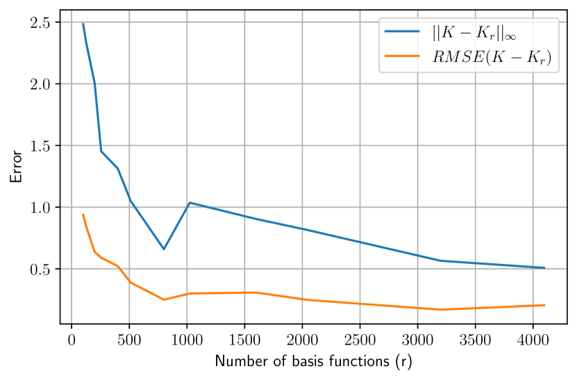
(a) Convergence of errors.

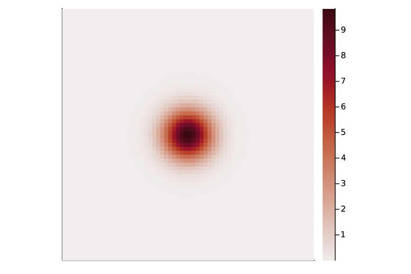
(b) True Kernel

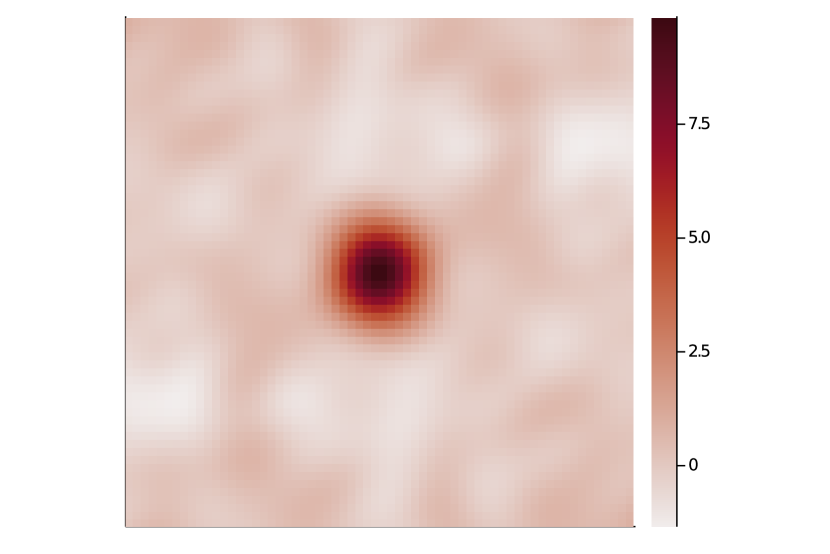
(c) Approximate kernel with
$r=512$ features.

Figure 1: Kernel approximation for $\sigma=0.2,\mu=10.0$.

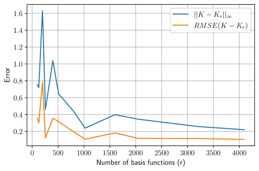
(a) Convergence of errors

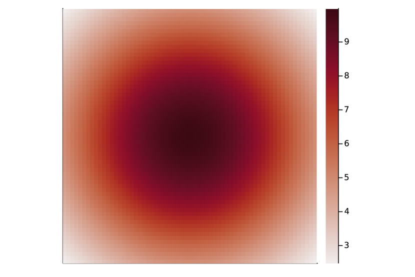
(b) True Kernel

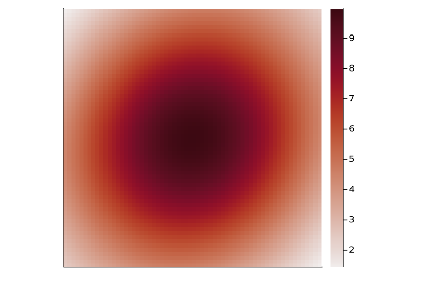
(c) Approximate kernel with
$r=512$ features.

Figure 2: Kernel approximation for $\sigma=1.25,\mu=10.0$.

We take the Lagrangian and terminal cost functions

$$L(t,x,v)=\frac{\|v\|^{2}}{2},\quad\psi(x)=10\|x-x_{\text{target}}\|^{2},\quad(t,x,v)\in(0,1)\times\mathbb{R}^{d}\times\mathbb{R}^{d},$$

where $x_{\text{target}}=0$. This choice corresponds to a model where crowd-averse agents travel from initial positions towards a target location, $x_{\text{target}}$. Finally, we sample $M=256$ initial positions from $\rho_{0}$.

In Figure 3 we plot the projections of agents’ trajectories on the first two dimensions when the repulsion radius is $\sigma=0.2$ and $d=2,50,100$. Analogously, we plot the agents trajectories for $\sigma=1.25$ and $d=2,50,100$ in Figure 4. Note that trajectories split more when $\sigma=0.2$, which corresponds to the case when agents are more sensitive to their immediate neighbors. Additionally, note that the terminal cost function enforces agents to reach the destination $x_{\text{target}}=0$. The 3D trajectories are plotted in Figure 5.

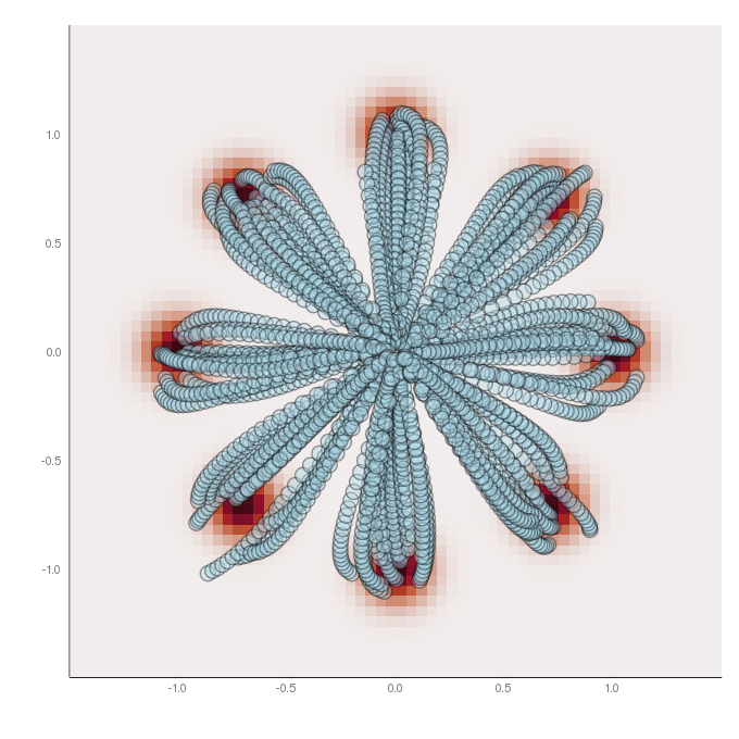
(a) $d=2,\sigma=0.2$.

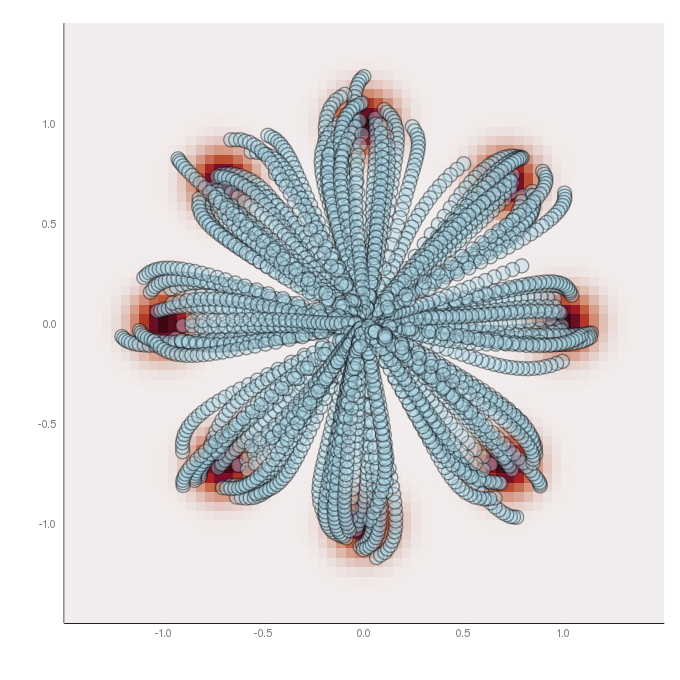
(b) $d=50,\sigma=0.2$.

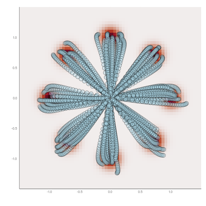
(c) $d=100,\sigma=0.2$.

Figure 3: Agents’ trajectories in experiments A for $\sigma=0.2$ plotted on the first two dimensions. Agents move from 8 Gaussian distributions (colored red) to the target point ($0,0$). Each plot shows the trajectories solved in different dimensions: (a) $d=2$, (b) $d=50$, (c) $d=100$.

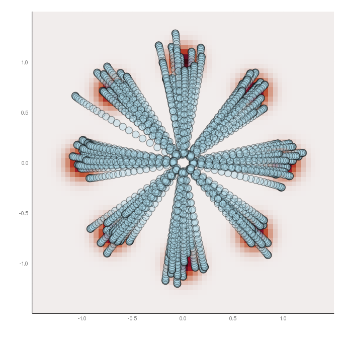
$d=2,\sigma=1.25$.

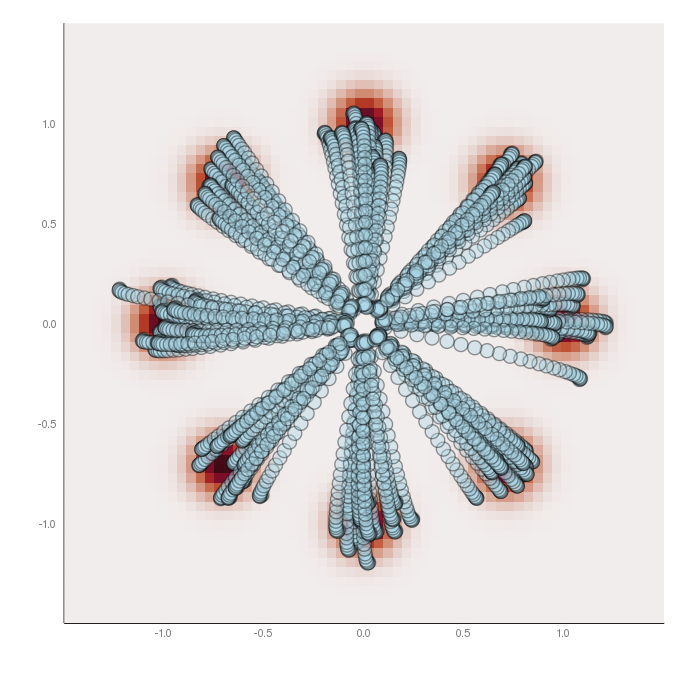
(a) $d=50,\sigma=1.25$.

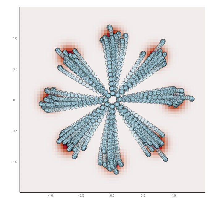
(b) $d=100,\sigma=1.25$.

Figure 4: Agents’ trajectories in experiments A for $\sigma=1.25$ plotted on the first two dimensions. Agents move from 8 Gaussian distributions (colored red) to the target point ($0,0$). Each plot shows the trajectories solved in different dimensions: (a) $d=2$, (b) $d=50$, (c) $d=100$.

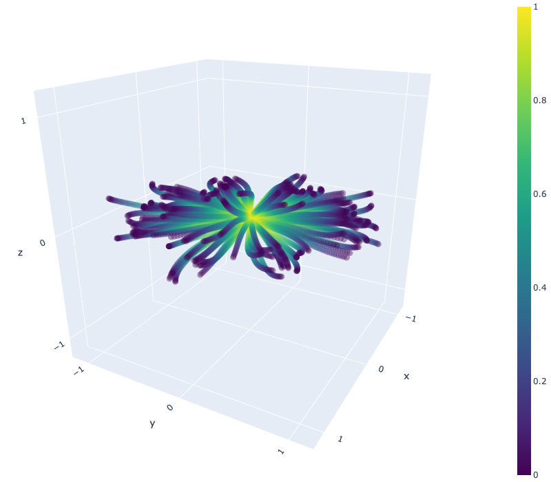
(a) 3D view.

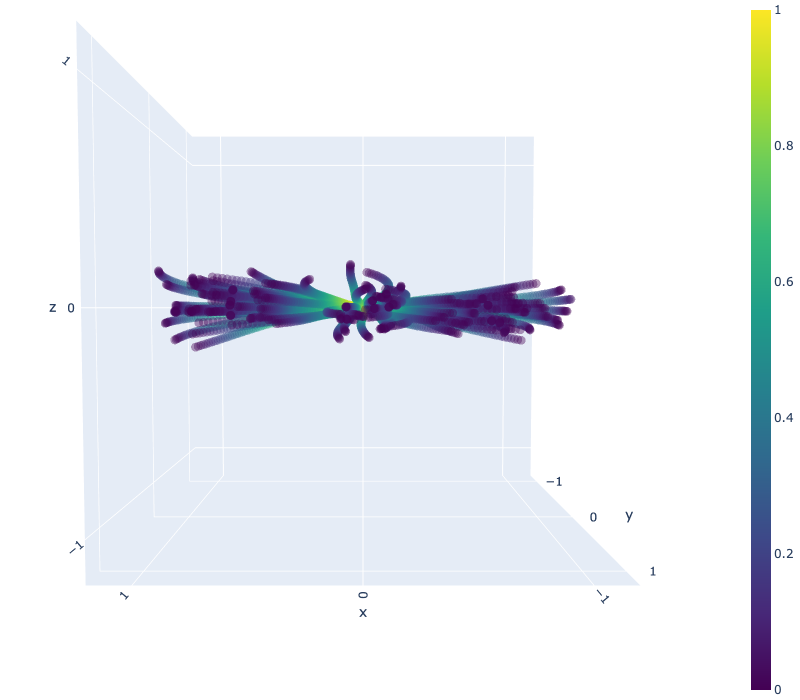
(b) XZ view.

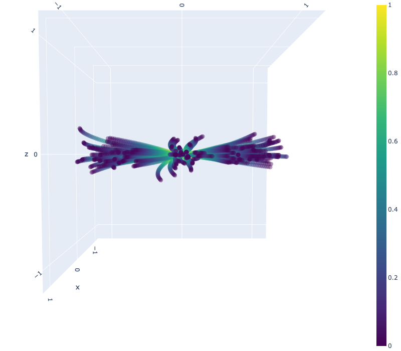
(c) YZ view.

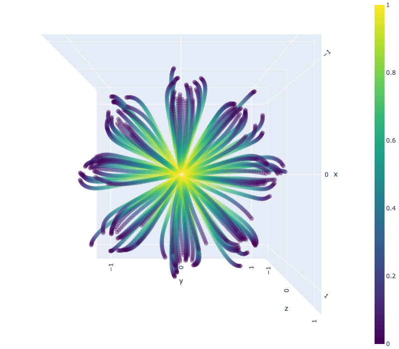
(d) Top view.

Figure 5: 3D plots of agents’ trajectories in experiments A with low-dimensional interactions (the first two dimensions) for $d=50$, ${\sigma}=0.2$. The plots show the first three dimensions of the trajectories. Each agent starts from $t=0$ (colored blue) to $t=1$ (colored yellow). The plots are from four different viewpoints. (a): 3D view, (b), (c): side views (XZ view and YZ view), (d): top view (XY view). The interactions of agents are only across the first two dimensions. Thus, while the agents spread in XY axis (see (d) for the top view), they move to the target point almost linearly in other axis (see (b) and (c) for the side views).

In Table 1 we report the population running cost

$$\frac{h}{M}\sum_{m=1}^{M}\sum_{l=1}^{N}L(s,{\mathbf{z}}_{x_{m}}[l],{\mathbf{v}}_{x_{m}}[l]),$$

interaction cost

$$h\sum_{l=1}^{N}\frac{1}{2M^{2}}\sum_{m,m^{\prime}=1}^{M}K_{r}({\mathbf{z}}_{x_{m}}[l],{\mathbf{z}}_{x_{m^{\prime}}}[l])=\frac{h}{2M^{2}}\sum_{l=1}^{N}\left(\sum_{i=1}^{r}\zeta_{i}({\mathbf{z}}_{x_{m}}[l])\right)^{2},$$

terminal cost

$$\frac{1}{M}\sum_{m=1}^{M}\psi(\mathbf{z}_{x_{m}}[N]),$$

and the total cost at the equilibrium.

$d$	$\sigma$	Running	Interaction	Terminal	Total
2	0.2	0.526	0.465	0.0108	1.10
2	1.25	0.621	3.57	0.00997	4.29
50	0.2	0.754	0.454	0.0116	1.32
50	1.25	0.825	3.58	0.0109	4.51
100	0.2	0.992	0.533	0.0140	1.67
100	1.25	1.11	3.26	0.0139	4.51

Table 1: Running, interaction, terminal, and total costs in experiments A.

5.2 Experiment B

In this set of experiments we assume that agents are initially distributed according to

$$\rho_{0}(x)\propto\exp\left(-\frac{\|x-x_{\text{initial}}\|^{2}}{2\cdot 0.2^{2}}\right),\quad x\in\mathbb{R}^{d},$$

where $x_{\text{initial}}=(0,1,0,\cdots,0)\in\mathbb{R}^{d}$. Furthermore, we assume that the Lagrangian and terminal cost functions are

$$\begin{split}L(t,x,v)=&\frac{\|v\|^{2}}{4}+5\max\left(x^{\prime\top}\begin{bmatrix}1&0\\ 0&-5\end{bmatrix}x^{\prime},0\right),\quad\psi(x)=10\|x-x_{\text{target}}\|^{2},\end{split}$$

for $(t,x,v)\in(0,1)\times\mathbb{R}^{d}\times\mathbb{R}^{d}$, where $x_{\text{target}}=(0,-1,0,\cdots,0)$.

As before, we consider low-dimensional interactions with a kernel of the form 23. We take $\mu=50$ and $\sigma=1$. The approximation error and the approximate kernel for $r=512$ are plotted in Figure 6. As before, the plots are generated by evaluating the true kernel and the approximate kernel at points on a 2-dimensional grid.

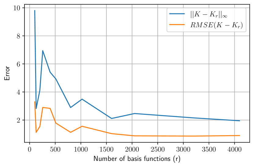
(a) Convergence of errors.

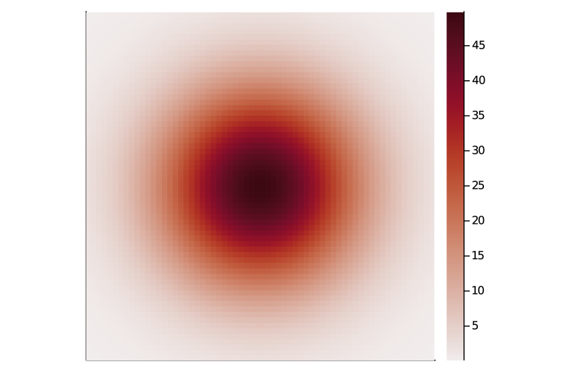
(b) True Kernel

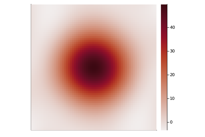
(c) Approximate kernel with
$r=512$ features.

Figure 6: Kernel approximation for $\sigma=1.0,\mu=50.0$.

Thus, in experiments B we model a crowd-averse population that travels from around an initial point, $x_{\text{initial}}$, to a target point, $x_{\text{target}}$, avoiding wedge shaped obstacles. The projections of agents’ trajectories on the first two dimensions are plotted in Figure 7.

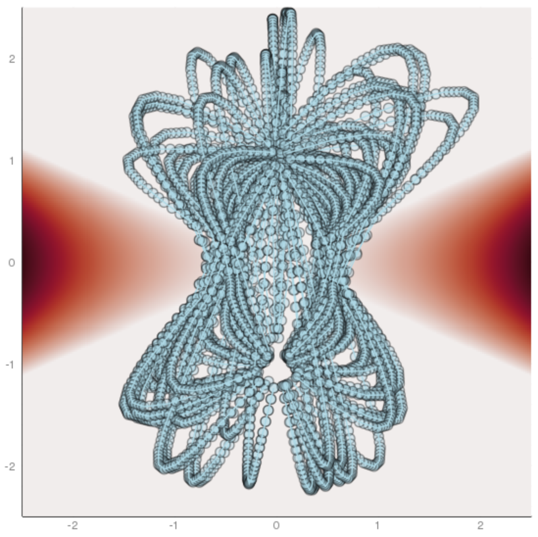
(a) $d=2$.

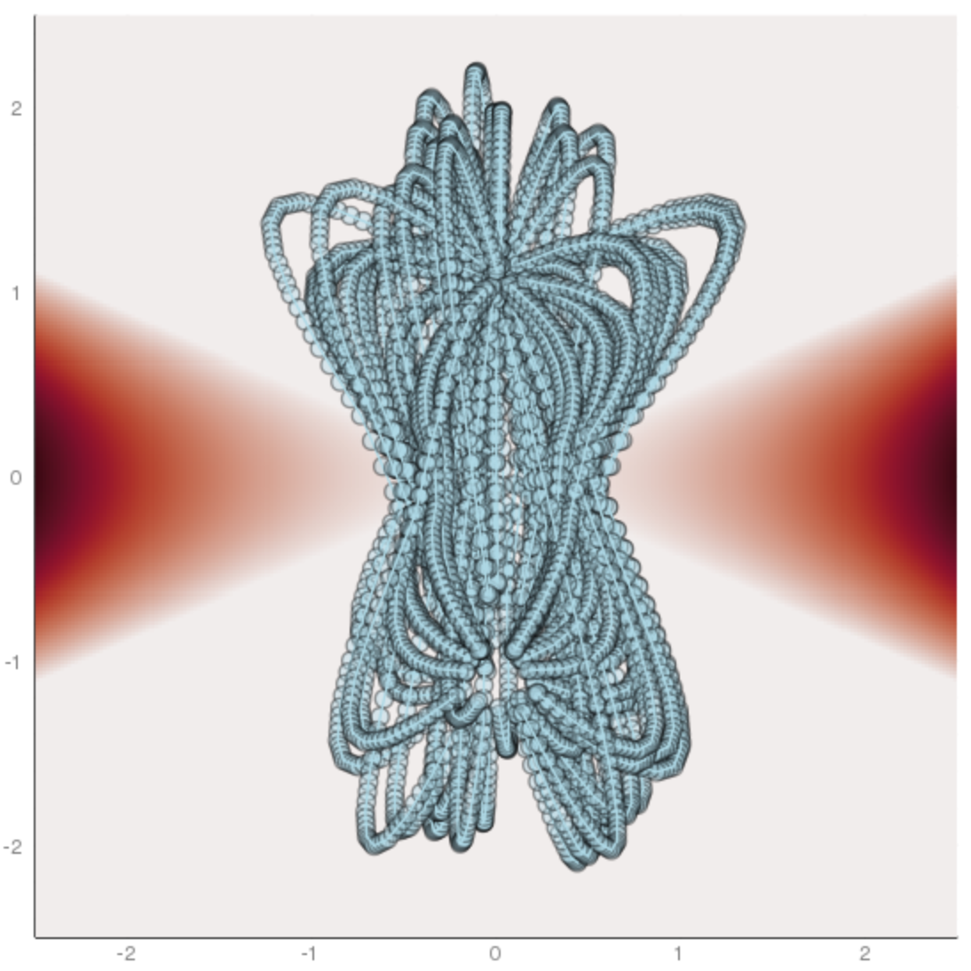
(b) $d=50$.

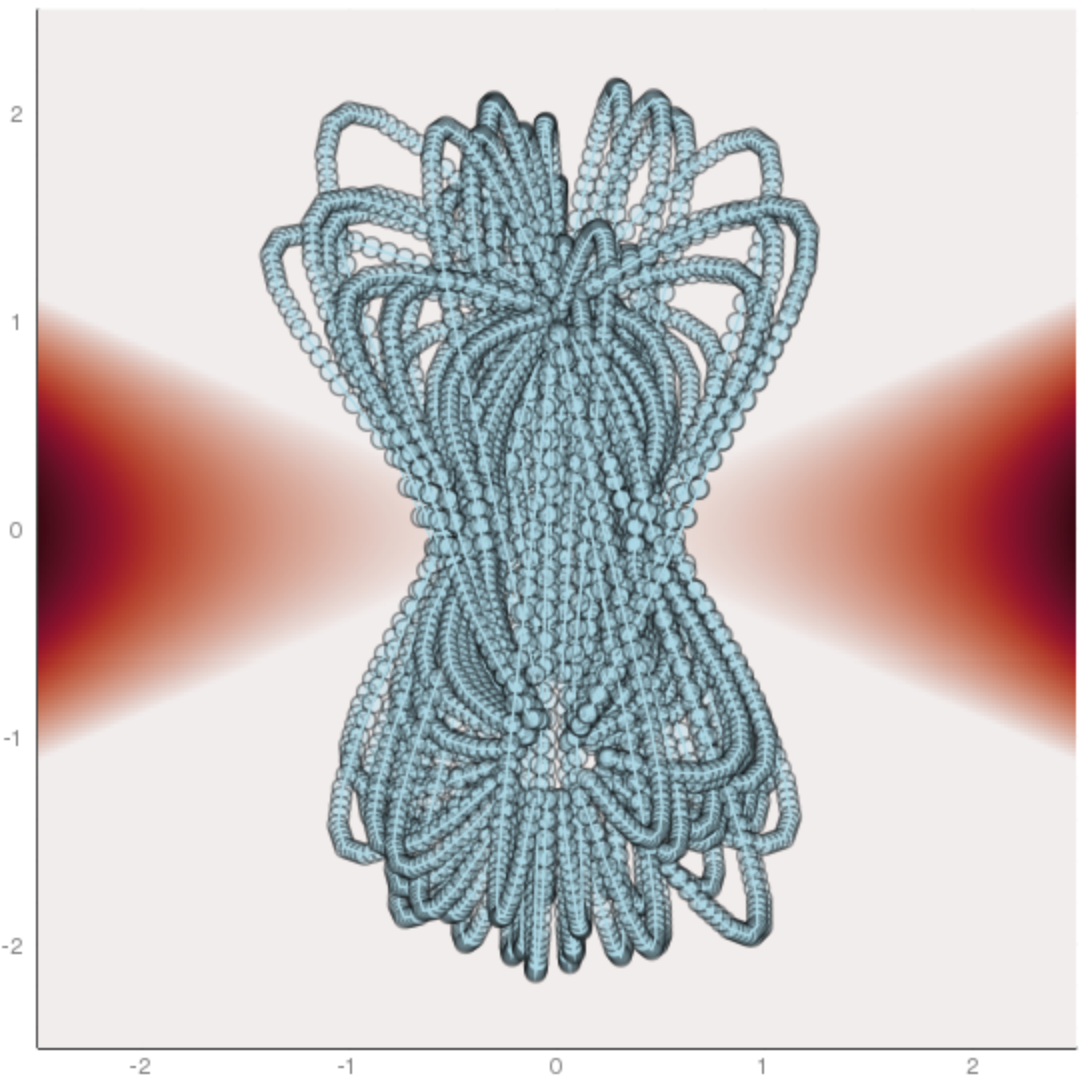
(c) $d=100$.

Figure 7: Agents’ trajectories in experiments B plotted on the first two dimensions. Agents move from the initial distribution (near $(0,1)$) to the target point ($0,-1$) while avoiding the obstacle (colored red). Each plot shows the trajectories solved in different dimensions: (a) $d=2$, (b) $d=50$, (c) $d=100$.

Note that the trajectories split at close to the initial and target points, demonstrating the crowd-averse behavior of the agents. On the other hand, obstacles force the agents to converge at the bottleneck.

We plot the 3D trajectories in Figure 8 and report running, interaction, terminal, and total costs in Table 2.

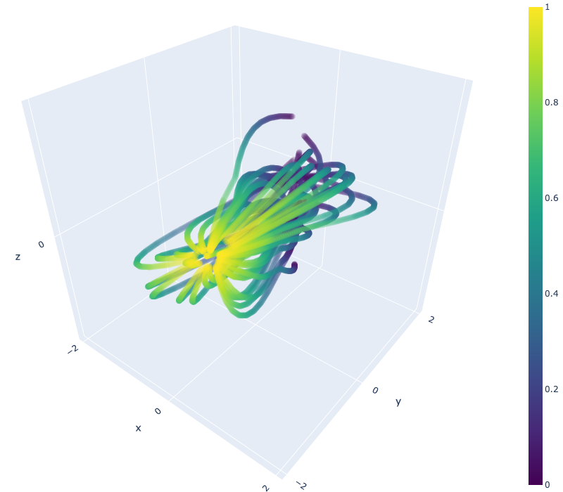
(a) 3D view.

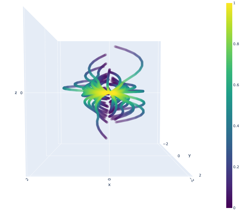
(b) XZ view.

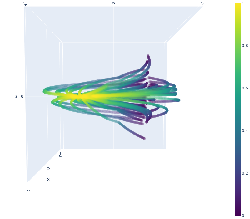
(c) YZ view.

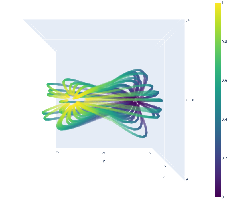
(d) Top view.

Figure 8: 3D plots of Agents’ trajectories with low-dimensional interactions in experiments B for $d=50$. The plots show the first three dimensions of the trajectories. Each agent starts from $t=0$ (colored blue) to $t=1$ (colored yellow) while avoiding the obstacle (see Figure 7). The plots are from four different viewpoints. (a): 3D view (the target point is at the lower-left side of the plot and the initial distributions are at the top-right side of the plot), (b), (c): side views (XZ view and YZ view), (d): top view (XY view). The interactions of agents are only across the first two dimensions. Thus, while the agents spread in XY axis (see (d) for the top view), they move to the target point almost linearly in other axis (see (c) for the side view).

$d$	Running	Interaction	Terminal	Total
2	3.72	12.2	0.388	16.3
50	2.63	15.4	0.533	18.6
100	2.86	14.8	0.567	18.3

Table 2: Running, interaction, terminal, and total costs in experiments B.

5.3 Experiment C

In experiments A, B we consider high-dimensional problems with low-dimensional interactions. Here, we perform experiments similar to A but with full-dimensional interactions to demonstrate the efficiency of our method for higher-dimensional interactions as well.

Thus, we assume that we are in the same setup as in A with the only difference that $K$ is a full-dimensional interaction 16 with $\sigma=\hat{\sigma}\cdot\sqrt{d/2}$, and $\mu=10$ and $\mu=1$ for $\hat{\sigma}=0.2$ and $\hat{\sigma}=1.25$, respectively. Here, $\hat{\sigma}$ is a dimensionless repulsion radius. Indeed, since for $\rho_{0}$ in 22 the variance of constituent Gaussians is the same across dimensions, the average distance between agents scales with a factor $\sqrt{d}$ near the centers of these Gaussians. Hence, if we used the same repulsion radius across all dimensions, the effective interaction would be different, and it would be hard to interpret the results. By fixing a repulsion radius $\hat{\sigma}$ for $d=2$ and scaling it accordingly we make sure that the effective interaction is the same across all dimensions, and we should obtain similar equilibrium behavior.

The results for $\hat{\sigma}=0.2$ and $\hat{\sigma}=1.25$ are plotted in Figures 9 and 10, respectively.

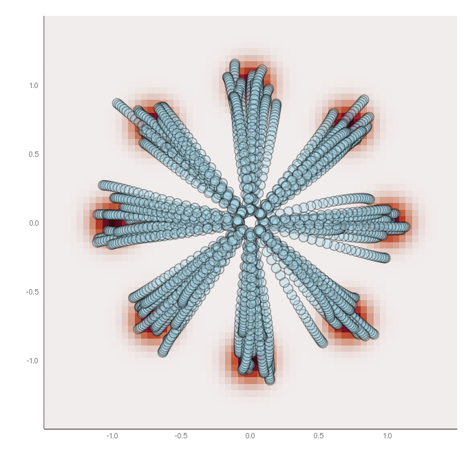
(a) $d=50,\mu=10,\hat{\sigma}=0.2$.

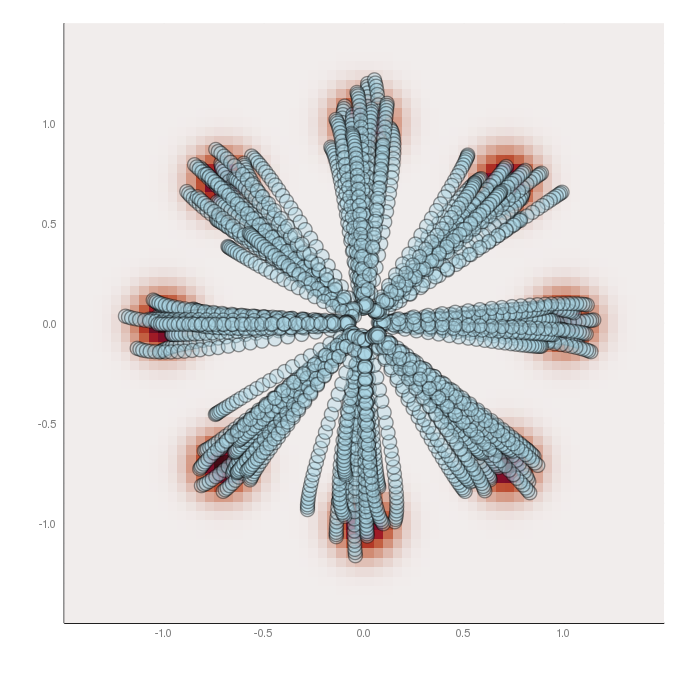
(b) $d=100,\mu=10,\hat{\sigma}=0.2$.

Figure 9: Agents’ trajectories in experiments C for $\hat{\sigma}=0.2$ plotted on the first two dimensions. Agents move from 8 Gaussian distributions (colored red) to the target point ($0,0$). Each plot shows the trajectories solved in different dimensions: (a) $d=50$, (b) $d=100$.

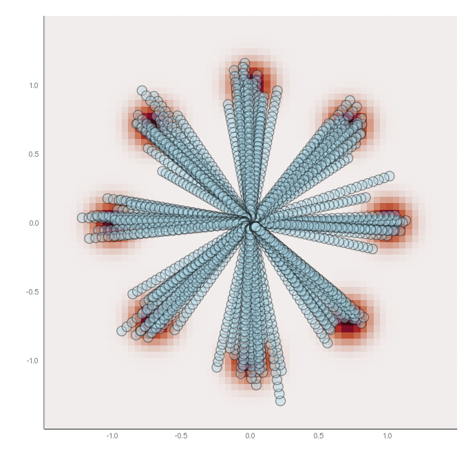
(a) $d=50,\mu=1,\hat{\sigma}=1.25$.

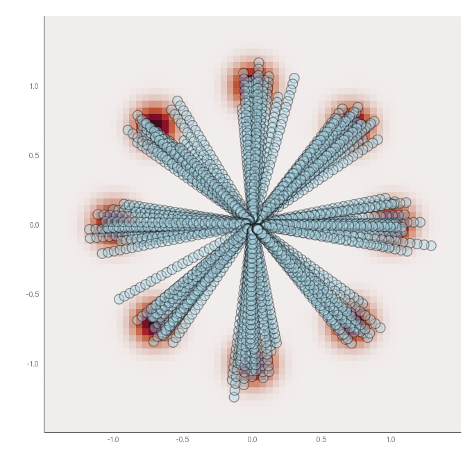
(b) $d=100,\mu=1,\hat{\sigma}=1.25$.

Figure 10: Agents’ trajectories in experiments C for $\hat{\sigma}=1.25$ plotted on the first two dimensions. Agents move from 8 Gaussian distributions (colored red) to the target point ($0,0$). Each plot shows the trajectories solved in different dimensions: (a) $d=50$, (b) $d=100$.

Note that the trajectories are almost straight lines when $\hat{\sigma}=1.25$. In Figures 11, 12, 13 we plot the original and approximate kernels to explain this phenomenon. More specifically, in Figures 11(a) and 12(a) we plot $K(x,0)$ and $K_{r}(x,0)$ along a random direction so that $|x|\leq 2.5$. Furthermore, in Figures 11(b) and 12(b) we plot the decay of the approximation error $K(x,\mu_{c})-K_{r}(x,\mu_{c})$ in $l^{\infty}$ and $l^{2}$ norms for $x$ sampled according to $\rho_{0}$, where $\mu_{c}$ is the center of one of the eight constituent Gaussians of $\rho_{0}$. Finally, we superimpose Figures 11(a) and 12(a) in Figure 13.

As we can see in Figures 12(a) and 13, the interaction kernel is almost flat for $\hat{\sigma}=1.25$ within the support of $\rho_{0}$. Hence, the interaction cost is approximately the same for all agents, which effectively decouples the agents leading to individual control problems with a purely quadratic cost. In the latter case, optimal trajectories are straight lines as follows from the Hopf-Lax theory [61, Section 3.3].

We plot the 3D trajectories in Figure 14 and report running, interaction, terminal, and total costs in Table 3.

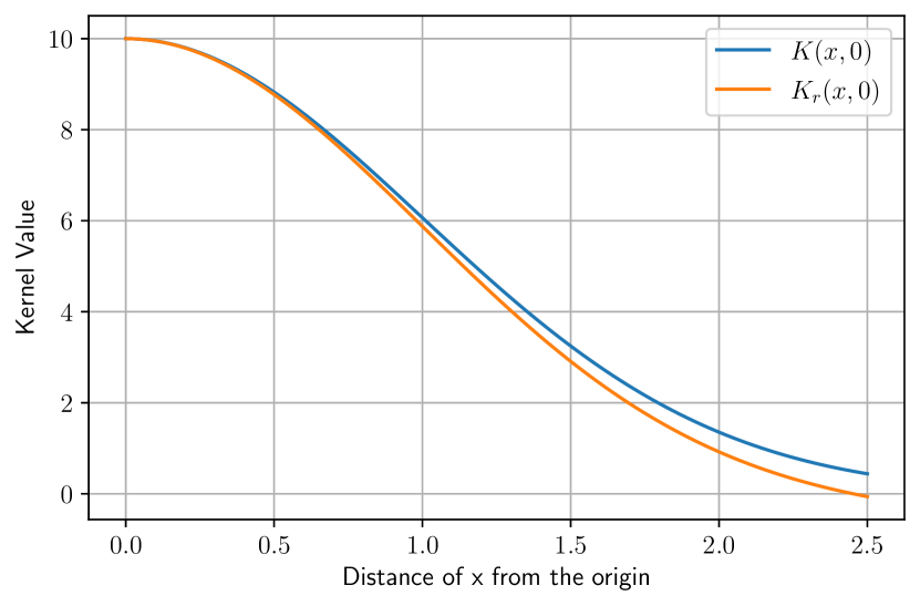
(a) Kernel values along a random direction $r=512$

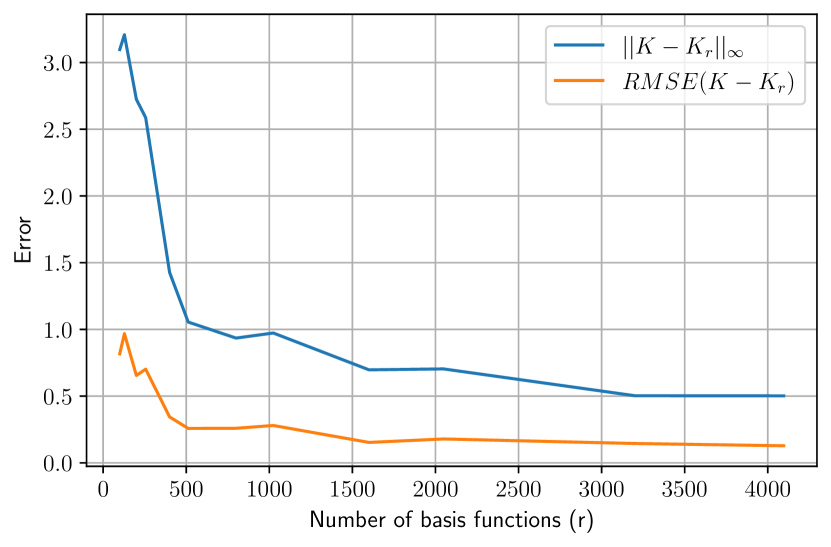
(b) Convergence of errors

Figure 11: Kernel approximation for $d=50,\hat{\sigma}=0.2,\mu=10.0$.

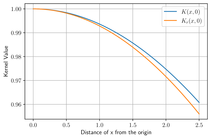
(a) Kernel values along a random direction $r=512$

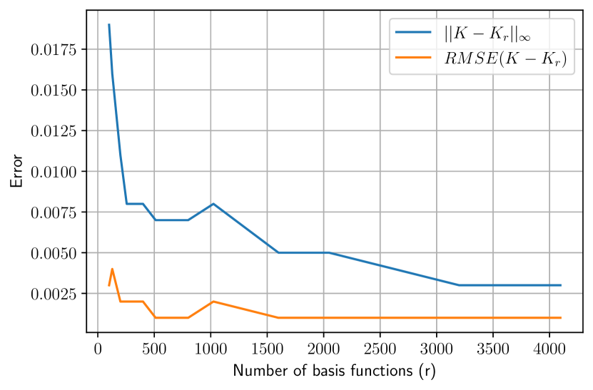
(b) Convergence of errors

Figure 12: Kernel approximation for $d=100,\hat{\sigma}=1.25,\mu=1.0$.

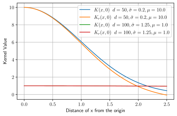
Figure 13: Kernel values along a random ray for $r=512,\hat{\sigma}=0.2,1.25$

$d$	$\hat{\sigma}$	$\mu$	running	interaction	terminal	total
50	0.2	10	1.05	1.96	0.0192	3.20
50	1.25	1	0.674	0.492	0.00340	1.20
100	0.2	10	1.21	2.59	0.0177	3.97
100	1.25	1	0.912	0.495	0.00458	1.45

Table 3: Running, interaction, terminal, and total costs in experiments C.

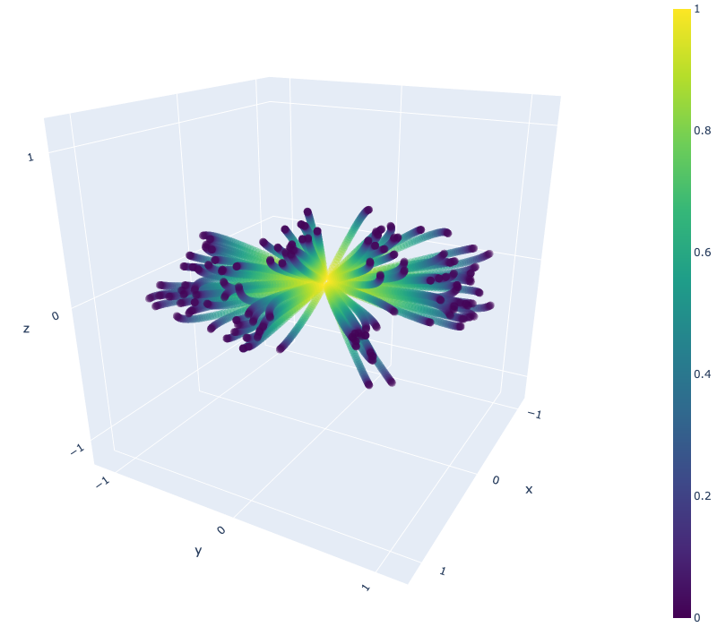
(a) 3D view.

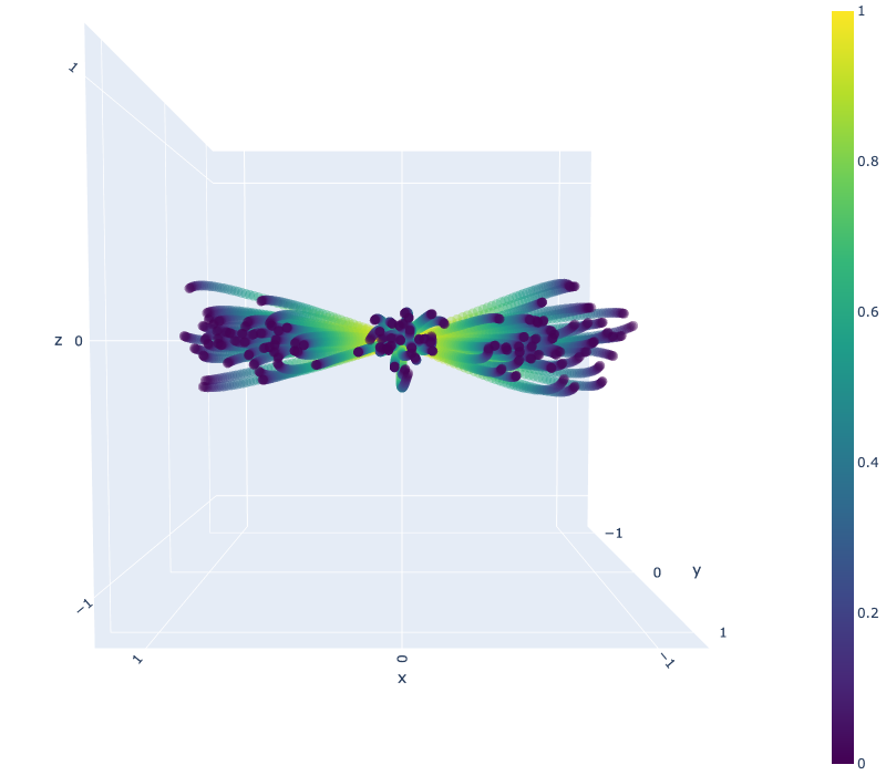
(b) XZ view.

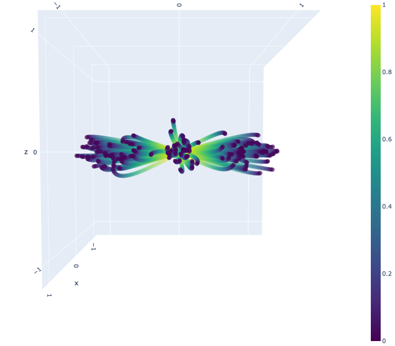
(c) YZ view.

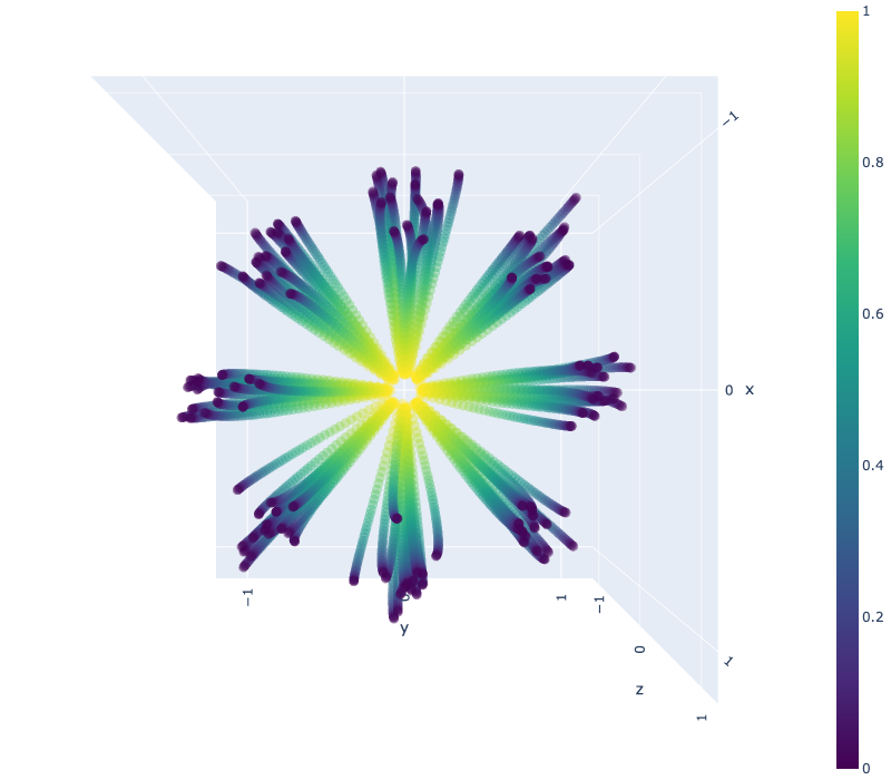
(d) Top view.

Figure 14: 3D plots of Agents’ trajectories in experiments C with full-dimensional interactions for $d=50$, $\hat{\sigma}=0.2$. The plots show the first three dimensions of the trajectories. Each agent starts from $t=0$ (colored blue) to $t=1$ (colored yellow). The plots are from four different viewpoints. (a): 3D view, (b), (c): side views (XZ view and YZ view), (d): top view (XY view). Because of full-dimensional interactions, the spread of agents’ trajectories can be observed from every viewpoints.

6 Conclusion

We propose an efficient solution approach for high-dimensional nonlocal MFG systems utilizing random-feature expansions of interaction kernels. We thus bypass the costly state space discretizations of interaction terms and allow for straightforward extensions of virtually any single-agent trajectory optimization algorithm to the mean-field setting. As an example, we extend the direct transcription approach in optimal control to the mean-field setting. Our numerical results demonstrate the efficiency of our method by solving MFG problems in up to a hundred-dimensional state space. To the best of our knowledge, this is the first instance of solving such high-dimensional problems with non-deep-learning techniques.

Future work involves the extension of our method to affine controls arising in, e.g., quadrotors [62], as well as alternative trajectory generation methods that involve deep learning [57, 48].

Compact feature space representations of interaction kernels are also valuable for inverse problems. In a forthcoming paper [63], we recover the interaction kernel from data by postulating its feature space expansion.

Furthermore, note that feature space expansions of the kernel are not related to the mean-field idealization. Thus, we plan to investigate applications of our method to possibly heterogeneous multi-agent problems where the number of agents is not large enough for the mean-field approximation to be valid [53, 54].

Finally, an interesting and challenging question is the convergence analysis of the primal-dual algorithm 21 described in Section 4. We anticipate analysis methods developed in [41] to be useful for this question.

Appendix

Derivation of 7.

Assume that $v(t,x)$ is a smooth vector field. For every $x\in\mathbb{R}^{d}$ denote by $z_{x}(t)$ the solution of the ODE

$$\dot{z}_{x}(t)=v(t,z_{x}(t)),\quad z_{x}(0)=x.$$ (24)

If agents are distributed according to $\rho_{0}$ at time $t=0$ and follow the flow in 24, their distribution, $\rho(t,x)$, satisfies the continuity equation

$$\partial_{t}\rho(t,x)+\nabla\cdot\left(\rho(t,x)v(t,x)\right)=0,\quad\rho(0,x)=\rho_{0}(x).$$

Now assume that $\phi_{a}$ is the solution of 8. From the optimal control theory we have that

$$\begin{split}&\int_{\mathbb{R}^{d}}\phi_{a}(0,x)d\rho_{0}(x)\\ \leq&\int_{\mathbb{R}^{d}}\left[\int_{0}^{T}\left\{L(t,z_{x}(t),v(t,z_{x}(t)))+\sum_{i=1}^{r}a_{i}(t)\zeta_{i}(z_{x}(t))\right\}dt+\psi(z_{x}(T))\right]d\rho_{0}(x)\\ =&\int_{\mathbb{R}^{d}}\int_{0}^{T}\left\{L(t,x,v(t,x))+\sum_{i=1}^{r}a_{i}(t)\zeta_{i}(x)\right\}dtd\rho(t,x)+\int_{\mathbb{R}^{d}}\psi(x)d\rho(T,x),\end{split}$$

where equality holds for $(\rho,v)=(\rho_{a},v_{a})$ given by

$$\begin{split}&v_{a}(t,x)=-\nabla_{p}H(t,x,\nabla\phi_{a}(t,x))\\ &\partial_{t}\rho_{a}(t,x)-\nabla\cdot\left(\rho_{a}(t,x)\nabla_{p}H(t,x,\nabla\phi_{a}(t,x))\right)=0,\quad\rho_{a}(0,x)=\rho_{0}(x).\end{split}$$ (25)

Summarizing, we obtain that

$$\begin{split}\int_{\mathbb{R}^{d}}\phi_{a}(0,x)d\rho_{0}(x)=&\inf_{\begin{subarray}{c}\partial_{t}\rho+\nabla\cdot(\rho v)=0\\ \rho(0,x)=\rho_{0}(x)\end{subarray}}\int_{\mathbb{R}^{d}}\int_{0}^{T}L(t,x,v(t,x))dtd\rho(t,x)\\ &+\int_{\mathbb{R}^{d}}\int_{0}^{T}\sum_{i=1}^{r}a_{i}(t)\zeta_{i}(x)\rho(t,x)dtdx+\int_{\mathbb{R}^{d}}\psi(x)d\rho(T,x),\end{split}$$ (26)

where the equality holds for $(\rho,v)=(\rho_{a},v_{a})$ in 25. Applying perturbation analysis for optimization problems [64, Proposition 4.12] we obtain

$$\frac{\delta}{\delta a_{i}(t)}\int_{R^{d}}\phi_{a}(0,x)d\rho_{0}(x)=\int_{\mathbb{R}^{d}}\zeta_{i}(x)d\rho_{a}(t,x)=\int_{\mathbb{R}^{d}}\zeta_{i}(z_{x,a}(t))d\rho_{0}(x),$$ (27)

where $z_{x,a}$ is the solution of 24 for the optimal control $v=v_{a}$.

Now we are in the position for proving the equivalence between 6 and 7. We have that

$$\int_{\mathbb{R}^{d}}K_{r}(x,y)d\rho(t,y)=\sum_{i=1}^{r}a_{i}(t)\zeta_{i}(x),$$ (28)

where

$$a_{i}(t)=\sum_{j=1}^{r}k_{ij}\int_{\mathbb{R}^{d}}\zeta_{j}(y)d\rho(t,y).$$ (29)

Therefore, $(\phi,\rho)$ solve 6 if and only if $(\phi,\rho)=(\phi_{a},\rho_{a})$ for $a$ satisfying 29. Furthermore, 27 yields that 29 is precisely equivalent to

$$a(t)={\mathbf{K}}\frac{\delta}{\delta a(t)}\int_{R^{d}}\phi_{a}(0,x)d\rho_{0}(x)$$

which leads to 7. ∎

References

-
[1]
M. Huang, R. P. Malhamé, P. E. Caines,
Large population
stochastic dynamic games: closed-loop McKean-Vlasov systems and the
Nash certainty equivalence principle, Commun. Inf. Syst. 6 (3) (2006)
221–251.
URL http://projecteuclid.org/euclid.cis/1183728987 -
[2]
M. Huang, P. E. Caines, R. P. Malhamé,
Large-population cost-coupled
LQG problems with nonuniform agents: individual-mass behavior and
decentralized -Nash equilibria, IEEE Trans. Automat. Control
52 (9) (2007) 1560–1571.
doi:10.1109/TAC.2007.904450.
URL https://doi.org/10.1109/TAC.2007.904450 -
[3]
J.-M. Lasry, P.-L. Lions,
Jeux à champ moyen. I.
Le cas stationnaire, C. R. Math. Acad. Sci. Paris 343 (9) (2006) 619–625.
doi:10.1016/j.crma.2006.09.019.
URL https://doi.org/10.1016/j.crma.2006.09.019 -
[4]
J.-M. Lasry, P.-L. Lions,
Jeux à champ moyen. II.
Horizon fini et contrôle optimal, C. R. Math. Acad. Sci. Paris
343 (10) (2006) 679–684.
doi:10.1016/j.crma.2006.09.018.
URL https://doi.org/10.1016/j.crma.2006.09.018 -
[5]
J.-M. Lasry, P.-L. Lions, Mean
field games, Jpn. J. Math. 2 (1) (2007) 229–260.
doi:10.1007/s11537-007-0657-8.
URL https://doi.org/10.1007/s11537-007-0657-8 -
[6]
Y. Achdou, F. J. Buera, J.-M. Lasry, P.-L. Lions, B. Moll,
Partial differential equation
models in macroeconomics, Philos. Trans. R. Soc. Lond. Ser. A Math. Phys.
Eng. Sci. 372 (2028) (2014) 20130397, 19.
doi:10.1098/rsta.2013.0397.
URL https://doi.org/10.1098/rsta.2013.0397 -
[7]
Y. Achdou, J. Han, J.-M. Lasry, P.-L. Lions, B. Moll,
Income and wealth distribution in
macroeconomics: A continuous-time approach, Working Paper 23732, National
Bureau of Economic Research (August 2017).
doi:10.3386/w23732.
URL http://www.nber.org/papers/w23732 - [8] O. Guéant, J.-M. Lasry, P.-L. Lions, Mean field games and applications, in: Paris-Princeton lectures on mathematical finance 2010, Springer, 2011, pp. 205–266.
- [9] D. A. Gomes, L. Nurbekyan, E. A. Pimentel, Economic models and mean-field games theory, IMPA Mathematical Publications, Instituto Nacional de Matemática Pura e Aplicada (IMPA), Rio de Janeiro, 2015.
- [10] D. Firoozi, P. E. Caines, An optimal execution problem in finance targeting the market trading speed: An mfg formulation, in: 2017 IEEE 56th Annual Conference on Decision and Control (CDC), 2017, pp. 7–14.
-
[11]
P. Cardaliaguet, C.-A. Lehalle,
Mean field game of controls
and an application to trade crowding, Math. Financ. Econ. 12 (3) (2018)
335–363.
doi:10.1007/s11579-017-0206-z.
URL https://doi.org/10.1007/s11579-017-0206-z - [12] P. Casgrain, S. Jaimungal, Algorithmic trading in competitive markets with mean field games, SIAM News 52 (2).
- [13] A. De Paola, V. Trovato, D. Angeli, G. Strbac, A mean field game approach for distributed control of thermostatic loads acting in simultaneous energy-frequency response markets, IEEE Transactions on Smart Grid 10 (6) (2019) 5987–5999. doi:10.1109/TSG.2019.2895247.
-
[14]
A. C. Kizilkale, R. Salhab, R. P. Malhamé,
An
integral control formulation of mean field game based large scale
coordination of loads in smart grids, Automatica 100 (2019) 312 – 322.
doi:https://doi.org/10.1016/j.automatica.2018.11.029.
URL http://www.sciencedirect.com/science/article/pii/S0005109818305612 - [15] D. A. Gomes, J. Saúde, A mean-field game approach to price formation in electricity markets, arXiv:1807.07088.
- [16] Z. Liu, B. Wu, H. Lin, A mean field game approach to swarming robots control, in: 2018 Annual American Control Conference (ACC), IEEE, 2018, pp. 4293–4298.
- [17] K. Elamvazhuthi, S. Berman, Mean-field models in swarm robotics: a survey, Bioinspiration & Biomimetics 15 (1) (2019) 015001.
- [18] Y. Kang, S. Liu, H. Zhang, W. Li, Z. Han, S. Osher, H. V. Poor, Joint sensing task assignment and collision-free trajectory optimization for mobile vehicle networks using mean-field games, IEEE Internet of Things Journal 8 (10) (2021) 8488–8503. doi:10.1109/JIOT.2020.3047739.
- [19] Y. Kang, S. Liu, H. Zhang, Z. Han, S. Osher, H. V. Poor, Task selection and route planning for mobile crowd sensing using multi-population mean-field games, in: ICC 2021 - IEEE International Conference on Communications, 2021, pp. 1–6. doi:10.1109/ICC42927.2021.9500261.
- [20] W. Lee, S. Liu, H. Tembine, S. Osher, Controlling propagation of epidemics via mean-field games, UCLA CAM preprint:20-19.
- [21] S. L. Chang, M. Piraveenan, P. Pattison, M. Prokopenko, Game theoretic modelling of infectious disease dynamics and intervention methods: a review, Journal of Biological Dynamics 14 (1) (2020) 57–89.
- [22] E. Weinan, J. Han, Q. Li, A mean-field optimal control formulation of deep learning, Research in the Mathematical Sciences 6 (1) (2019) 10.
- [23] X. Guo, A. Hu, R. Xu, J. Zhang, Learning mean-field games, in: Advances in Neural Information Processing Systems, 2019, pp. 4967–4977.
- [24] R. Carmona, M. Laurière, Z. Tan, Linear-quadratic mean-field reinforcement learning: convergence of policy gradient methods, arXiv:1910.04295.
- [25] P. Cardaliaguet, Notes on mean field games, https://www.ceremade.dauphine.fr/ cardaliaguet/ (2013).
-
[26]
Y. Achdou, P. Cardaliaguet, F. Delarue, A. Porretta, F. Santambrogio,
Mean field games, Vol. 2281
of Lecture Notes in Mathematics, Springer, Cham; Centro Internazionale
Matematico Estivo (C.I.M.E.), Florence, [2020] ©2020, edited by
Pierre Cardaliaguet and Alessio Porretta, Fondazione CIME/CIME Foundation
Subseries.
doi:10.1007/978-3-030-59837-2.
URL https://doi.org/10.1007/978-3-030-59837-2 -
[27]
D. A. Gomes, E. A. Pimentel, V. Voskanyan,
Regularity theory for
mean-field game systems, SpringerBriefs in Mathematics, Springer, [Cham],
2016.
doi:10.1007/978-3-319-38934-9.
URL https://doi.org/10.1007/978-3-319-38934-9 - [28] A. Cesaroni, M. Cirant, Introduction to variational methods for viscous ergodic mean-field games with local coupling, in: Contemporary research in elliptic PDEs and related topics, Vol. 33 of Springer INdAM Ser., Springer, Cham, 2019, pp. 221–246.
- [29] R. Carmona, F. Delarue, Probabilistic theory of mean field games with applications. I, Vol. 83 of Probability Theory and Stochastic Modelling, Springer, Cham, 2018, mean field FBSDEs, control, and games.
- [30] R. Carmona, F. Delarue, Probabilistic theory of mean field games with applications. II, Vol. 84 of Probability Theory and Stochastic Modelling, Springer, Cham, 2018, mean field games with common noise and master equations.
-
[31]
A. Bensoussan, J. Frehse, P. Yam,
Mean field games and mean
field type control theory, SpringerBriefs in Mathematics, Springer, New
York, 2013.
doi:10.1007/978-1-4614-8508-7.
URL https://doi.org/10.1007/978-1-4614-8508-7 -
[32]
P. Cardaliaguet, F. Delarue, J.-M. Lasry, P.-L. Lions,
The master equation and the
convergence problem in mean field games, Vol. 201 of Annals of Mathematics
Studies, Princeton University Press, Princeton, NJ, 2019.
doi:10.2307/j.ctvckq7qf.
URL https://doi.org/10.2307/j.ctvckq7qf - [33] W. Gangbo, A. R. Mészáros, C. Mou, J. Zhang, Mean field games master equations with non-separable hamiltonians and displacement monotonicity (2021). arXiv:2101.12362.
-
[34]
Y. Achdou, P. Mannucci, C. Marchi, N. Tchou,
Deterministic mean
field games with control on the acceleration and state constraints: extended
version, working paper or preprint (Nov. 2021).
URL https://hal.archives-ouvertes.fr/hal-03408825 -
[35]
L. Nurbekyan, One-dimensional,
non-local, first-order stationary mean-field games with congestion: a
Fourier approach, Discrete Contin. Dyn. Syst. Ser. S 11 (5) (2018)
963–990.
doi:10.3934/dcdss.2018057.
URL https://doi.org/10.3934/dcdss.2018057 -
[36]
L. Nurbekyan, J. Saúde, Fourier
approximation methods for first-order nonlocal mean-field games, Port. Math.
75 (3-4) (2018) 367–396.
doi:10.4171/PM/2023.
URL https://doi.org/10.4171/PM/2023 -
[37]
S. Liu, M. Jacobs, W. Li, L. Nurbekyan, S. J. Osher,
Computational methods for
first-order nonlocal mean field games with applications, SIAM Journal on
Numerical Analysis 59 (5) (2021) 2639–2668.
arXiv:https://doi.org/10.1137/20M1334668, doi:10.1137/20M1334668.
URL https://doi.org/10.1137/20M1334668 - [38] S. Liu, L. Nurbekyan, Splitting methods for a class of non-potential mean field games, Journal of Dynamics & Games 8 (4) (2021) 467–486.
- [39] A. Rahimi, B. Recht, Random features for large-scale kernel machines, in: NIPS 2007, 2007, pp. 1177–1184.
-
[40]
P. Cardaliaguet, S. Hadikhanloo,
Learning in mean field games: the
fictitious play, ESAIM Control Optim. Calc. Var. 23 (2) (2017) 569–591.
doi:10.1051/cocv/2016004.
URL https://doi.org/10.1051/cocv/2016004 - [41] S. Hadikhanloo, Learning in anonymous nonatomic games with applications to first-order mean field games, arXiv: Optimization and Control.
-
[42]
S. Hadikhanloo, F. J. Silva,
Finite mean field games:
fictitious play and convergence to a first order continuous mean field game,
J. Math. Pures Appl. (9) 132 (2019) 369–397.
doi:10.1016/j.matpur.2019.02.006.
URL https://doi.org/10.1016/j.matpur.2019.02.006 - [43] J. F. Bonnans, P. Lavigne, L. Pfeiffer, Generalized conditional gradient and learning in potential mean field games (2021). arXiv:2109.05785.
-
[44]
F. Camilli, F. Silva, A
semi-discrete approximation for a first order mean field game problem, Netw.
Heterog. Media 7 (2) (2012) 263–277.
doi:10.3934/nhm.2012.7.263.
URL https://doi.org/10.3934/nhm.2012.7.263 -
[45]
E. Carlini, F. J. Silva, A fully
discrete semi-Lagrangian scheme for a first order mean field game problem,
SIAM J. Numer. Anal. 52 (1) (2014) 45–67.
doi:10.1137/120902987.
URL https://doi.org/10.1137/120902987 -
[46]
E. Carlini, F. J. Silva, A
semi-Lagrangian scheme for a degenerate second order mean field game
system, Discrete Contin. Dyn. Syst. 35 (9) (2015) 4269–4292.
doi:10.3934/dcds.2015.35.4269.
URL https://doi.org/10.3934/dcds.2015.35.4269 -
[47]
E. Carlini, F. J. Silva, On the
discretization of some nonlinear fokker–planck–kolmogorov equations and
applications, SIAM Journal on Numerical Analysis 56 (4) (2018) 2148–2177.
arXiv:https://doi.org/10.1137/17M1143022, doi:10.1137/17M1143022.
URL https://doi.org/10.1137/17M1143022 - [48] A. T. Lin, S. W. Fung, W. Li, L. Nurbekyan, S. J. Osher, Alternating the population and control neural networks to solve high-dimensional stochastic mean-field games, Proceedings of the National Academy of Sciences 118 (31).
-
[49]
H. Li, Y. Fan, L. Ying,
A
simple multiscale method for mean field games, Journal of Computational
Physics 439 (2021) 110385.
doi:https://doi.org/10.1016/j.jcp.2021.110385.
URL https://www.sciencedirect.com/science/article/pii/S0021999121002801 - [50] C. Mou, X. Yang, C. Zhou, Numerical methods for mean field games based on gaussian processes and fourier features (2021). arXiv:2112.05414.
-
[51]
J. Bezanson, A. Edelman, S. Karpinski, V. B. Shah,
Julia: A fresh approach to numerical
computing, SIAM review 59 (1) (2017) 65–98.
URL https://doi.org/10.1137/141000671 - [52] W. Rudin, Fourier analysis on groups, Vol. 121967, Wiley Online Library, 1962.
- [53] D. Onken, L. Nurbekyan, X. Li, S. W. Fung, S. Osher, L. Ruthotto, A neural network approach applied to multi-agent optimal control, in: 2021 European Control Conference (ECC), 2021, pp. 1036–1041.
- [54] D. Onken, L. Nurbekyan, X. Li, S. W. Fung, S. Osher, L. Ruthotto, A neural network approach for high-dimensional optimal control, arXiv preprint arXiv:2104.03270.
- [55] T. Nakamura-Zimmerer, Q. Gong, W. Kang, Adaptive deep learning for high-dimensional hamilton-jacobi-bellman equations, arXiv preprint arXiv:1907.05317.
- [56] C. Parkinson, D. Arnold, A. L. Bertozzi, S. Osher, A model for optimal human navigation with stochastic effects, arXiv:2005.03615.
- [57] L. Ruthotto, S. J. Osher, W. Li, L. Nurbekyan, S. W. Fung, A machine learning framework for solving high-dimensional mean field game and mean field control problems, Proceedings of the National Academy of Sciences 117 (17) (2020) 9183–9193.
- [58] D. Onken, S. Wu Fung, X. Li, L. Ruthotto, Ot-flow: Fast and accurate continuous normalizing flows via optimal transport, in: Proceedings of the AAAI Conference on Artificial Intelligence, Vol. 35, 2021.
- [59] P. J. Enright, B. A. Conway, Discrete approximations to optimal trajectories using direct transcription and nonlinear programming, Journal of Guidance, Control, and Dynamics 15 (4) (1992) 994–1002.
-
[60]
A. Chambolle, T. Pock, A
first-order primal-dual algorithm for convex problems with applications to
imaging, J. Math. Imaging Vision 40 (1) (2011) 120–145.
doi:10.1007/s10851-010-0251-1.
URL https://doi.org/10.1007/s10851-010-0251-1 - [61] L. C. Evans, Partial differential equations, Vol. 19 of Graduate Studies in Mathematics, American Mathematical Society, Providence, RI, 1998.
- [62] L. R. G. Carrillo, A. E. D. López, R. Lozano, C. Pégard, Modeling the quad-rotor mini-rotorcraft, in: Quad Rotorcraft Control, Springer, 2013, pp. 23–34.
- [63] Y. T. Chow, S. W. Fung, S. Liu, L. Nurbekyan, S. Osher, A numerical algorithm for inverse problem from partial boundary measurement arising from mean field game problem, arXiv preprint arXiv:2204.04851.
- [64] J. F. Bonnans, A. Shapiro, Perturbation analysis of optimization problems, Springer Series in Operations Research, Springer-Verlag, New York, 2000.