P3H-22-019, TTP22-012
The width difference in $B\!-\!\bar{B}\,$ mixing at order $\alpha_{s}$ and beyond

Abstract

We complete the calculation of the element $\Gamma_{12}^{q}$ of the decay matrix in $B_{q}-\bar{B}_{q}$ mixing, $q=d,s$, to order $\alpha_{s}$ in the leading power of the Heavy Quark Expansion. To this end we compute one- and two-loop contributions involving two four-quark penguin operators. Furthermore, we present two-loop QCD corrections involving a chromomagnetic operator and either a current-current or four-quark penguin operator. Such contributions are of order $\alpha_{s}^{2}$, i.e. next-to-next-to-leading-order. We also present one-loop and two-loop results involving two chromomagnetic operators which are formally of next-to-next-to-leading and next-to-next-to-next-to-leading-order, respectively. With our new corrections we obtain the Standard-Model prediction $\Delta\Gamma_{s}/\Delta M_{s}=(5.20\pm 0.69)\cdot 10^{-3}$ if $\Gamma_{12}^{s}$ is expressed in terms of the $\overline{\rm MS}$ b-quark mass, while we find $\Delta\Gamma_{s}/\Delta M_{s}=(4.70\pm 0.96)\cdot 10^{-3}$ instead for the use of the pole mass.

1 Introduction

The description of $B_{q}\!-\!\bar{B}{}_{q}\,$ mixing, where $q=d$ or $s$, involves two hermitian $2\times 2$ matrices, the mass matrix $M$ and the decay matrix $\Gamma$. Their off-diagonal elements $M_{12}^{q}$ and $\Gamma_{12}^{q}$ enter the observables related to $B_{q}\!-\!\bar{B}{}_{q}\,$ mixing, namely

$$\Delta M_{q} = M_{H}^{q}-M_{L}^{q}\,,$$

$$\Delta\Gamma_{q} = \Gamma_{L}^{q}-\Gamma_{H}^{q}\,,$$ (1)

$$\mbox{and~{}~{}}a_{\rm fs}^{q} = \mbox{Im}\frac{\Gamma_{12}^{q}}{M_{12}^{q}}\,.$$ (2)

Here $M_{L,H}$ and $\Gamma_{L,H}$ denote the masses and widths of the two eigenstates found by diagonalizing $M-i\Gamma/2$. The mass difference $\Delta M_{q}$ and the width difference $\Delta\Gamma_{q}$ are related to $M_{12}^{q}$ and $\Gamma_{12}^{q}$ as

$$\Delta M_{q} \simeq 2|M_{12}^{q}|,\qquad\qquad\frac{\Delta\Gamma_{q}}{\Delta M_{q}}\;=\;-\mbox{Re}\frac{\Gamma_{12}^{q}}{M_{12}^{q}}\,.$$ (3)

In the Standard Model (SM) the phase between $-\Gamma_{12}^{q}$ and $M_{12}^{q}$ is small, so that the CP asymmetry in flavor-specific decays, $a_{\rm fs}^{q}$, is much smaller than $\Delta\Gamma_{q}/\Delta M_{q}$ and further $\Delta\Gamma_{q}\simeq 2|\Gamma_{12}^{q}|$.

All results calculated in this paper equally apply to the $B_{s}$ and $B_{d}$ systems. For definiteness, we quote all formulae for the case of $B_{s}\!-\!\bar{B}{}_{s}\,$ mixing, the generalization to $B_{d}\!-\!\bar{B}{}_{d}\,$ mixing is found by replacing the elements $V_{qs}$, $q=u,c,t$, of the Cabibbo-Kobayashi-Maskawa (CKM) matrix by $V_{qd}$.

Currently, better theory predictions are needed for the case of $B_{s}\!-\!\bar{B}{}_{s}\,$ mixing to be competitive with the precise experimental values

$$\Delta M^{\rm exp}_{s} = (17.7656\pm 0.0057)\;\mbox{ps${}^{-1}\qquad$\cite[cite]{[\@@bibref{}{LHCb:2021moh}{}{}]}}\,,$$

$$\Delta\Gamma^{\rm exp}_{s} = (0.082\pm 0.005)\;\mbox{ps}^{-1}\qquad\hskip 15.00002pt\mbox{\cite[cite]{[\@@bibref{}{hfag}{}{}]}}\,,$$ (4)

where the quoted number for $\Delta\Gamma^{\rm exp}_{s}$ is derived from data of LHCb [3], CMS [4], ATLAS [5], CDF [6], and DØ [7].

$M_{12}^{s}$ probes virtual contributions of very heavy particles, while $\Gamma_{12}^{s}$ is mainly sensitive to new physics mediated by particles with masses below the electroweak scale. Nevertheless, a better theory prediction of $|\Gamma_{12}^{s}|$ also helps to quantify new physics in $M_{12}^{s}$: Both $\Delta M_{s}$ and $\Delta\Gamma_{s}$ are proportional to $|V_{ts}|^{2}$, where $V_{ts}$ is an element of the CKM matrix. $|V_{ts}|$ is calculated from (and is essentially identical to) $|V_{cb}|$ extracted from measured $b\to c\ell\nu$, $\ell=e,\mu$, branching ratios. The unfortunate discrepancy between the values for $|V_{cb}|$ found from inclusive and exclusive decays inflicts an uncertainty of order 15% on the predicted $\Delta M_{s}$. Now $V_{ts}$ cancels from $\Delta\Gamma_{s}/\Delta M_{s}$ in Eq. (3), so that the SM prediction of this ratio is not affected by the $V_{cb}$ controversy.

In this paper we address $\Gamma_{12}^{s}$ at leading order of the heavy-quark expansion (“leading power”), which expresses $\Gamma_{12}^{s}$ as a series in powers of $\Lambda_{\rm QCD}/m_{b}$. At this order one encounters only two physical $\Delta B=2$ operators, whose hadronic matrix elements have been calculated with high precision with lattice QCD [8]. These matrix elements are multiplied with Wilson coefficients which are calculated in perturbative QCD. The insufficient accuracy of the Wilson coefficients dominates the uncertainty of the SM prediction of $\Delta\Gamma_{q}$ [9, 10, 11, 12, 13, 14, 15], which exceeds the experimental error in Eq. (4). The perturbative calculation of power corrections to $\Gamma_{12}^{s}$ has been carried out to order $\alpha_{s}^{0}$ [16] and first lattice results for the associated hadronic matrix elements are also available [17].

The $|\Delta B|=1$ Hamiltonian $\mathcal{H}_{\textrm{eff}}^{|\Delta B|=1}$ comprises current-current operators with large coefficients $C_{1,2}$ and the four-quark penguin operators whose coefficients $C_{3-6}$ are small, with magnitudes well below 0.1, at the scale $\mu_{1}={\cal O}(m_{b})$ at which they enter $\Gamma_{12}^{s}$. At order $\alpha_{s}^{0}$, $\Gamma_{12}^{s}$ is composed of one-loop contributions proportional to $C_{j}C_{k}$ with $j,k\leq 6$. $\mathcal{H}_{\textrm{eff}}^{|\Delta B|=1}$ further involves the chromomagnetic penguin operator with coefficient $C_{8}\sim-0.16$, whose leading contribution is of order $\alpha_{s}$ and enters $\Gamma_{12}^{s}$ as products $C_{8}C_{k}$ with $k\leq 6$ . In Refs. [9, 10, 11, 12, 13, 14] the small coefficients $C_{3-6}$ have been formally treated as ${\cal O}(\alpha_{s})$. With this counting the one-loop terms with $C_{1,2}C_{3-6}$ contribute to next-to-leading order (NLO) and those involving two factors of $C_{3-6}$ are already part of the next-to-next-to-leading order (NNLO). First steps towards NNLO accuracy have been done in Refs. [13, 14] by calculating contribution proportional to the number of active quark flavors, i.e. loop diagrams with a closed fermion line.

As in Ref. [15] we use the conventional notion of “NLO” and “NNLO” in this paper and treat $C_{3-6}$ on the same footing as $C_{1,2}$. With this counting the NLO prediction of $\Gamma_{12}^{s}$ requires the calculation of the yet unknown two-loop contributions with one or two four-quark penguin operators. In this paper present several two-loop calculations, namely:

• penguin contributions proportional to the product of two $C_{3-6}$ coefficients. This contribution completes the prediction of $\Gamma_{12}^{s}$ to order $\alpha_{s}$, which is NLO in the above-mentioned conventional power counting. The corresponding one-loop corrections have been computed in Ref. [16]. Two-loop contributions with one current-current and one four-quark penguin operator have been calculated in Ref. [15].

• the contribution proportional to the product of $C_{8}$ and one of $C_{1-6}$. The calculated one-loop and two-loop terms contribute to NLO and NNLO, respectively. The piece of the one-loop correction proportional to the number $N_{f}$ of active quark flavors (stemming from diagrams with closed quark loops) has been computed in Ref. [14].

• the contribution proportional to $C_{8}^{2}$. Here the one-loop contribution is already of NNLO and not yet available in the literature, except for the $\alpha_{s}^{2}N_{f}$ part [14]. We further provide results for the two-loop term which is N³LO.

As in Ref. [15] we use the CMM basis [18] for the $|\Delta B|=1$ operators and calculate the two-loop QCD corrections as an expansion in

$$z = \frac{m_{c}^{2}}{m_{b}^{2}}$$ (5)

up to linear order.

The paper is organized as follows: In the next Section we briefly discuss the operator bases of the $|\Delta B|=1$ and $|\Delta B|=2$ theories. Afterwards, in Section 3 we provide some details of our calculation and in particular describe the matching procedure for the case of dimensionally regularized infra-red singularities. Analytic result for all new matching coefficients are listed in Section 4 and we present our numerical result for $\Delta\Gamma_{s}$ in Section 5. Section 6 contains our conclusions. In the Appendix we provide results for the renormalization constants relevant for the operator mixing in the $|\Delta B|=2$ theory.

2 Operator bases

The framework of our calculation is identical to the one used in Ref. [15] and thus in the following we repeat only the essential formulae needed to compute the width difference. The new contributions considered in this paper require an extension of the $|\Delta B|=2$ operator basis which is discussed in more detail.

For the effective $|\Delta B|=1$ theory we use the weak Hamiltonian

$$\mathcal{H}_{\textrm{eff}}^{|\Delta B|=1} = \frac{4G_{F}}{\sqrt{2}}\left[-\,\lambda^{s}_{t}\Big{(}\sum_{i=1}^{6}C_{i}Q_{i}+C_{8}Q_{8}\Big{)}-\lambda^{s}_{u}\sum_{i=1}^{2}C_{i}(Q_{i}-Q_{i}^{u})\right.$$ (6)

$$\phantom{\frac{4G_{F}}{\sqrt{2}}\Big{[}}\left.+\,V_{us}^{\ast}V_{cb}\,\sum_{i=1}^{2}C_{i}Q_{i}^{cu}+V_{cs}^{\ast}V_{ub}\,\sum_{i=1}^{2}C_{i}Q_{i}^{uc}\right]+\mbox{h.c.}\,,$$

where explicit expressions for the (physical and evanescent) operators can be found in Ref. [18]. $Q_{1},Q_{1}^{{(u,cu,uc)}},Q_{2}$ and $Q_{2}^{{(u,cu,uc)}}$ are current-current and $Q_{3},\ldots,Q_{6}$ are four-quark penguin operators. $Q_{8}$ is the chromomagnetic penguin operator. In Eq. (6) we have introduced the quantities $\lambda^{s}_{a}=V_{as}^{\ast}V_{ab}$, $a=u,c,t,$ which contain the CKM matrix elements. Furthermore, we have used $\lambda^{s}_{t}=-\lambda^{s}_{c}-\lambda^{s}_{u}$ and $G_{F}$ is the Fermi constant. Our two-loop calculations involve one-loop diagrams with counterterms to the physical operators in Eq. (6) and these counterterms comprise both physical and evanescent operators.

As mentioned in the Introduction, we specify our discussion to $b\to s$ decays relevant for $B_{s}\!-\!\bar{B}{}_{s}\,$ mixing. The corresponding expressions for $B_{d}\!-\!\bar{B}{}_{d}\,$ mixing are obtained by replacing $V_{as}$ with $V_{ad}$. Using the optical theorem we can relate $\Gamma_{12}^{s}$ to the $\bar{B}_{s}\to B_{s}$ forward scattering amplitude:

$$\Gamma_{12}^{s} = \frac{1}{2M_{B_{s}}}\,\mbox{Abs}\langle B_{s}|i\int{\rm d}^{4}x\,\,T\,\,{\cal H}_{\rm eff}^{\Delta B=1}(x){\cal H}_{\rm eff}^{\Delta B=1}(0)|\bar{B}_{s}\rangle\,,$$ (7)

where “Abs” stands for the absorptive part and $T$ is the time ordering operator. Note that $\Gamma_{12}^{s}$ encodes the information of the inclusive decay rate into final states common to $B_{s}$ and $\bar{B}_{s}$. Following Ref. [9] we decompose $\Gamma_{12}^{s}$ as

$$\Gamma_{12}^{s} = -(\lambda_{c}^{s})^{2}\Gamma^{cc}_{12}-2\lambda_{c}^{s}\lambda_{u}^{s}\Gamma_{12}^{uc}-(\lambda_{u}^{s})^{2}\Gamma^{uu}_{12}\,.$$ (8)

Let us now discuss the effective $|\Delta B|=2$ theory. To leading power in $1/m_{b}$ it is convenient to introduce the following four operators

$$Q = \bar{s}_{i}\gamma^{\mu}\,(1-\gamma^{5})\,b_{i}\;\bar{s}_{j}\gamma_{\mu}\,(1-\gamma^{5})\,b_{j}\,,$$

$$\widetilde{Q} = \bar{s}_{i}\gamma^{\mu}\,(1-\gamma^{5})\,b_{j}\;\bar{s}_{j}\gamma_{\mu}\,(1-\gamma^{5})\,b_{i}\,,$$

$$\widetilde{Q}_{S} = \bar{s}_{i}\,(1+\gamma^{5})\,b_{j}\;\bar{s}_{j}\,(1+\gamma^{5})\,b_{i}\,$$

$$Q_{S} = \bar{s}_{i}\,(1+\gamma^{5})\,b_{i}\;\bar{s}_{j}\,(1+\gamma^{5})\,b_{j}\,,$$ (9)

where $i,j$ are color indices. In four space-time dimensions there are only two independent operators which we choose as $Q$ and $\widetilde{Q}_{S}$ since we have (for $D=4$) $Q=\widetilde{Q}$ and

$$Q_{S} = -{\alpha_{1}}\widetilde{Q}_{S}-\frac{1}{2}{\alpha_{2}}Q+R_{0}\,,$$ (10)

where $R_{0}$ describes $1/m_{b}$-suppressed contributions to $\Gamma_{12}^{s}$ [16]. $\alpha_{1,2}$ are QCD correction factors which ensure that the $\overline{\rm MS}$ renormalized matrix element $\langle R_{0}\rangle$ has the desired power suppression [9, 12].

Using the Heavy Quark Expansion (HQE) it is thus possible to write $\Gamma_{12}^{ab}$ in Eq. (8) as

$$\Gamma_{12}^{ab} = \frac{G_{F}^{2}m_{b}^{2}}{24\pi M_{B_{s}}}\left[H^{ab}(z)\langle B_{s}|Q|\bar{B}_{s}\rangle+\widetilde{H}^{ab}_{S}(z)\langle B_{s}|\widetilde{Q}_{S}|\bar{B}_{s}\rangle\right]+\ldots\,$$ (11)

with $z=(m_{c}^{\rm pole}/m_{b}^{\rm pole})^{2}$ and the ellipses denoting higher-order terms in $\Lambda_{\rm QCD}/m_{b}$. Here $z$ is defined in terms of pole quark masses. Later we will trade $z$ for the ratio of $\overline{\rm MS}$ masses which leads to a better behavior of the perturbative series. $H^{ab}$ and $\widetilde{H}^{ab}_{S}$ are ultra-violet and infra-red finite matching coefficients which we decompose as follows

$$H{}^{ab}(z) = H^{(c)\,{ab}}(z)+H^{({c}p)\,{ab}}(z)+H^{(p)\,{ab}}(z)\,,$$

$$\widetilde{H}_{S}^{ab}(z) = \widetilde{H}_{S}^{(c)\,{ab}}(z)+\widetilde{H}_{S}^{({c}p)\,{ab}}(z)+\widetilde{H}_{S}^{(p)\,{ab}}(z)\,,$$ (12)

where the superscript “(c)” denotes the contributions with two current-current operators $Q_{1,2}$ or $Q_{1,2}^{(u,cu,uc)}$, “(cp)” refers to those with one operator $Q_{1,2}$ or $Q_{1,2}^{(u,cu,uc)}$ and one (four-quark or chromomagnetic) penguin operator $Q_{3-6,8}$ and “(p)” labels the terms involving two penguin operators. In this paper we present new contributions to $H^{(p)\,{ab}}$ and $\widetilde{H}_{S}^{(p)\,{ab}}(z)$ up to two-loop order.

At intermediate steps (i.e. in $D=4-2\epsilon$ dimensions) of our calculation it is convenient to use all four operators of Eq. (9) together with evanescent operators with two or three Dirac matrix structures given by [9, 19]

$$E_{1}^{(1)} = \widetilde{Q}-Q\,,$$

$$E_{2}^{(1)} = \bar{s}_{i}\gamma^{\mu}\gamma^{\nu}\gamma^{\rho}\,{(1-\gamma_{5})}\,{b}_{j}\;\bar{s}_{j}\gamma_{\mu}\gamma_{\nu}\gamma_{\rho}\,{(1-\gamma_{5})}\,{b}_{i}-(16-4\epsilon)\widetilde{Q}\,,$$

$$E_{3}^{(1)} = \bar{s}_{i}\gamma^{\mu}\gamma^{\nu}\gamma^{\rho}\,{(1-\gamma_{5})}\,{b}_{i}\;\bar{s}_{j}\gamma_{\mu}\gamma_{\nu}\gamma_{\rho}\,{(1-\gamma_{5})}\,{b}_{j}-(16-4\epsilon)Q\,,$$

$$E_{4}^{(1)} = \bar{s}_{i}\gamma^{\mu}\gamma^{\nu}\,{(1+\gamma_{5})}\,{b}_{j}\;\bar{s}_{j}\gamma_{\nu}\gamma_{\mu}\,{(1+\gamma_{5})}\,{b}_{i}+(8-8\epsilon)Q_{s}\,,$$

$$E_{5}^{(1)} = \bar{s}_{i}\gamma^{\mu}\gamma^{\nu}\,{(1+\gamma_{5})}\,{b}_{i}\;\bar{s}_{j}\gamma_{\nu}\gamma_{\mu}\,{(1+\gamma_{5})}\,{b}_{j}+(8-8\epsilon)\widetilde{Q}_{s}\,.$$ (13)

The ${\cal O}(\epsilon)$ parts in Eq. (13) are chosen such that the Fierz symmetry of the renormalized $|\Delta B|=2$ amplitudes extends to $D$ dimensions [20] and ${\cal O}(\epsilon^{2})$ terms, which are important for a three-loop (NNLO) calculation, have been omitted. Furthermore, we remark that the five evanescent operators in Eq. (13) are needed in order to determine the renormalization constants responsible for the operator mixing in the $|\Delta B|=2$ theory, see Appendix A.

Contribution			Maximal number of $\gamma$ matrices needed
			for the two-loop calculation
$Q_{1,2}$	$\times$	$Q_{1,2}$	$5\times 5$
$Q_{1,2}$	$\times$	$Q_{3-6}$	$5\times 5$
$Q_{3-6}$	$\times$	$Q_{3-6}$	$9\times 9$
$Q_{1,2}$	$\times$	$Q_{8}$	$3\times 3$
$Q_{3,6}$	$\times$	$Q_{8}$	$7\times 7$
$Q_{8}$	$\times$	$Q_{8}$	$5\times 5$

Table 1: Maximal number of $\gamma$ matrices which appear in the calculation of two-loop corrections to the various contributions involving current-current and penguin operators.

 

In our calculation we encounter further evanescent $|\Delta B|=2$ operators, since in intermediate steps Dirac structures with up to nine different $\gamma$ matrices can appear. In Tab. 1 we list the maximal number of $\gamma$ matrices for each pair of $|\Delta B|=1$ operators. It is easily obtained by inspecting the corresponding one-loop diagrams with one physical and one evanescent operator from Eqs. (9) and (13), respectively, or two-loop diagrams with two physical operators. We define the additional evanescent operators as

$$E_{1}^{(2)} = \bar{s}_{i}\gamma^{\mu_{1}}\ldots\gamma^{\mu_{5}}\,{(1-\gamma_{5})}\,{b}_{j}\;\bar{s}_{j}\gamma_{\mu_{1}}\ldots\gamma_{\mu_{5}}\,{(1-\gamma_{5})}\,{b}_{i}-(256+{e}_{1}^{(2)}\epsilon)\tilde{Q}\,,$$

$$E_{2}^{(2)} = \bar{s}_{i}\gamma^{\mu_{1}}\ldots\gamma^{\mu_{5}}\,{(1-\gamma_{5})}\,{b}_{i}\;\bar{s}_{j}\gamma_{\mu_{1}}\ldots\gamma_{\mu_{5}}\,{(1-\gamma_{5})}\,{b}_{j}-(256+{e}_{2}^{(2)}\epsilon)Q\,,$$

$$E_{3}^{(2)} = \bar{s}_{i}\gamma^{\mu_{1}}\ldots\gamma^{\mu_{4}}\,{(1+\gamma_{5})}\,{b}_{i}\;\bar{s}_{j}\gamma_{\mu_{1}}\ldots\gamma_{\mu_{4}}\,{(1+\gamma_{5})}\,{b}_{j}-(128+{e}_{3,1}^{(2)}\epsilon)\tilde{Q}_{S}$$

$$\mbox{}-(128+{e}_{3,2}^{(2)}\epsilon)Q_{S}\,,$$

$$E_{4}^{(2)} = \bar{s}_{i}\gamma^{\mu_{1}}\ldots\gamma^{\mu_{4}}\,{(1+\gamma_{5})}\,{b}_{j}\;\bar{s}_{j}\gamma_{\mu_{1}}\ldots\gamma_{\mu_{4}}\,{(1+\gamma_{5})}\,{b}_{i}-(128+{e}_{4,1}^{(2)}\epsilon)\tilde{Q}_{S}$$

$$\mbox{}-(128+{e}_{4,2}^{(2)}\epsilon)Q_{S}\,,$$

$$E_{1}^{(3)} = \bar{s}_{i}\gamma^{\mu_{1}}\ldots\gamma^{\mu_{7}}\,{(1-\gamma_{5})}\,{b}_{j}\;\bar{s}_{j}\gamma_{\mu_{1}}\ldots\gamma_{\mu_{7}}\,{(1-\gamma_{5})}\,{b}_{i}-(4096+{e}_{1}^{(3)}\epsilon)\tilde{Q},$$

$$E_{2}^{(3)} = \bar{s}_{i}\gamma^{\mu_{1}}\ldots\gamma^{\mu_{7}}\,{(1-\gamma_{5})}\,{b}_{i}\;\bar{s}_{j}\gamma_{\mu_{1}}\ldots\gamma_{\mu_{7}}\,{(1-\gamma_{5})}\,{b}_{j}-(4096+{e}_{2}^{(3)}\epsilon)Q,$$

$$E_{3}^{(3)} = \bar{s}_{i}\gamma^{\mu_{1}}\ldots\gamma^{\mu_{6}}\,{(1+\gamma_{5})}\,{b}_{i}\;\bar{s}_{j}\gamma_{\mu_{1}}\ldots\gamma_{\mu_{6}}\,{(1+\gamma_{5})}\,{b}_{j}-(2048+{e}_{3,1}^{(3)}\epsilon)\tilde{Q}_{S}$$

$$\mbox{}-(2048+{e}_{3,2}^{(3)}\epsilon)Q_{S},$$

$$E_{4}^{(3)} = \bar{s}_{i}\gamma^{\mu_{1}}\ldots\gamma^{\mu_{6}}\,{(1+\gamma_{5})}\,{b}_{j}\;\bar{s}_{j}\gamma_{\mu_{1}}\ldots\gamma_{\mu_{6}}\,{(1+\gamma_{5})}\,{b}_{i}-(2048+{e}_{4,1}^{(3)}\epsilon)\tilde{Q}_{S}$$

$$\mbox{}-(2048+{e}_{4,2}^{(3)}\epsilon)Q_{S}\,,$$

$$E_{1}^{(4)} = \bar{s}_{i}\gamma^{\mu_{1}}\ldots\gamma^{\mu_{9}}\,{(1-\gamma_{5})}\,{b}_{j}\;\bar{s}_{j}\gamma_{\mu_{1}}\ldots\gamma_{\mu_{9}}\,{(1-\gamma_{5})}\,{b}_{i}-(65536+{e}_{1}^{(4)}\epsilon)\tilde{Q},$$

$$E_{2}^{(4)} = \bar{s}_{i}\gamma^{\mu_{1}}\ldots\gamma^{\mu_{9}}\,{(1-\gamma_{5})}\,{b}_{i}\;\bar{s}_{j}\gamma_{\mu_{1}}\ldots\gamma_{\mu_{9}}\,{(1-\gamma_{5})}\,{b}_{j}-(65536+{e}_{2}^{(4)}\epsilon)Q,$$

$$E_{3}^{(4)} = \bar{s}_{i}\gamma^{\mu_{1}}\ldots\gamma^{\mu_{8}}\,{(1+\gamma_{5})}\,{b}_{i}\;\bar{s}_{j}\gamma_{\mu_{1}}\ldots\gamma_{\mu_{8}}\,{(1+\gamma_{5})}\,{b}_{j}-(32768+{e}_{3,1}^{(4)}\epsilon)\tilde{Q}_{S}$$

$$\mbox{}-(32768+{e}_{3,2}^{(4)}\epsilon)Q_{S},$$

$$E_{4}^{(4)} = \bar{s}_{i}\gamma^{\mu_{1}}\ldots\gamma^{\mu_{8}}\,{(1+\gamma_{5})}\,{b}_{j}\;\bar{s}_{j}\gamma_{\mu_{1}}\ldots\gamma_{\mu_{8}}\,{(1+\gamma_{5})}\,{b}_{i}-(32768+{e}_{4,1}^{(4)}\epsilon)\tilde{Q}_{S}$$ (14)

$$\mbox{}-(32768+{e}_{4,2}^{(4)}\epsilon)Q_{S}\,,$$

where for our calculation the values of ${e}_{j}^{(k)}$,${e}_{j,l}^{(k)}$, which parametrize the ${\cal O}(\epsilon)$ terms in the definition of the evanescent operators are irrelevant since the operators in Eq. (14) do not appear in one-loop counterterm contributions. These numbers, however, become important at NNLO to fully specify the renormalization scheme at this order.

3 Calculation and Matching

The setup which we use for our calculation has already been described in Ref. [15]. For convenience of the reader we repeat the essential steps and stress the differences in the following.

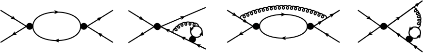
Figure 1: Sample Feynman diagrams contributing to Eq. (7) to the orders considered in this paper. From top to bottom they contribute to the $Q_{3-6}\times Q_{3-6}$, $Q_{1,2}\times Q_{8}$, $Q_{3,6}\times Q_{8}$, and $Q_{8}\times Q_{8}$ pieces of ${\cal H}_{\rm eff}^{\Delta B=1}(x){\cal H}_{\rm eff}^{\Delta B=1}(0)$ in Eq. (7), with the blobs denoting the corresponding current-current or penguin operators.

 

Figure 1 shows typical one- and two-loop Feynman diagrams for the new contributions considered in this paper. The displayed diagrams correspond to the $|\Delta B|=1$ side of the matching equation. In addition, one needs the one-loop diagrams with a gluon dressing the $\Delta B=2$ operators $Q$ and $\tilde{Q}_{S}$ to determine the desired Wilson coefficients $H^{ab}$ and $\widetilde{H}^{ab}_{S}$ in Eqs. (11) and (12). We perform the calculation for a generic QCD gauge parameter which drops out in the final result for each matching coefficient and thereby provides a non-trivial check of our calculation. The counterterms to the $\Delta B=1$ operators and the gauge coupling $g_{s}$ in the Feynman diagrams exemplified in Fig. 1 are all evaluated at the renormalization scale $\mu_{1}$. Conversely, operators and couplings on the $|\Delta B|=2$ side are evaluated at the scale $\mu_{2}$. The unphysical $\mu_{1}$ dependence of $H^{ab}(z)$ and $\widetilde{H}_{S}^{ab}(z)$ diminishes order-by-order in perturbation theory and can be used to assess the accuracy of the calculated result. The $\mu_{2}$ dependence of $H^{ab}(z)$ and $\widetilde{H}_{S}^{ab}(z)$, however, cancels with the $\mu_{2}$ dependence of the hadronic matrix element, which enters the lattice-continuum matching. For calculational convenience we first choose $\mu_{1}=\mu_{2}$ and implement the separation $\mu_{1}\not=\mu_{2}$ with the help of renormalization group techniques.

We pursue two different approaches to treat the four-quark amplitudes. The first one is based on tensor integrals combined with various manipulations of the Dirac structures and relies on FeynCalc [21, 22, 23] and Fermat [24]. The so-obtained formulae are then exported to FORM [25].

For the contribution $Q_{3-6}\times Q_{3-6}$ routines are needed which can handle tensor integrals up to rank 6. The second approach is based on projectors (see Appendix of Ref. [15]) which allows taking traces. Thus, one only has to deal with scalar expressions. However, one needs to calculate products of two traces with up to 18 $\gamma$ matrices in each trace. We find that both approaches lead to the same expressions for the amplitude with two $\Delta B=1$ operators once the latter is expressed in terms of tree-level $\Delta B=2$ matrix elements.

For the reduction of the $\Delta B=1$ amplitude we use FIRE [26] with symmetries from LiteRed [27, 28] and obtain four two-loop master integrals. Their evaluation as an expansion in $\epsilon$ is straightforward.

The amplitudes in the $|\Delta B|=1$ and $|\Delta B|=2$ theories contain both ultra-violet and infra-red singularities. The former are cured with parameter, quark field, and operator renormalization. We use the one-loop counterterms for $\alpha_{s}$ in the $\overline{\rm MS}$ scheme and renormalize the charm quark in the one-loop expression in the on-shell (or pole) scheme. The renormalization of the bottom quark, which we also renormalize on-shell, is only needed for the contributions involving $Q_{8}$. We also perform the renormalization of the external quark fields in the $\overline{\rm MS}$ scheme. The counterterms needed for the renormalization of the $\Delta B=1$ operator mixing can be taken from the literature [29]. The renormalization constants of the $\Delta B=2$ part are given in Appendix A.

In order to regulate the infra-red singularities two possibilities come to mind: One can either introduce a (small) gluon mass, $m_{g}$, or instead use dimensional regularization.

The choice $m_{g}\not=0$ is conceptually simpler and has the advantage that after renormalization the $\Delta B=1$ and $\Delta B=2$ amplitudes are separately finite and one can take the limit $D\to 4$, which eliminates all evanescent operators before matching the two theories. Furthermore, it is possible to use four-dimensional relations in order to arrive at a minimal operator basis. However, a finite gluon mass breaks gauge invariance and thus, in general, additional counterterms have to be introduced for its restoration. In our application the two-loop $\Delta B=1$ amplitudes with four-quark operators do not involve three-gluon vertices, and thus it is safe to regulate the infra-red divergences with $m_{g}\not=0$. However, at three-loop level this is not the case. Furthermore, the two-loop corrections with two $Q_{8}$ operators also contain infra-red divergences in the non-abelian part.

Regulating the infra-red divergences dimensionally using the same regulator $\epsilon$ as for the ultra-violet divergences has the advantage that the loop integrals are simpler. However, the matching has to be performed with divergent quantities in $D\not=4$ dimensions. As a consequence lower-order corrections have to be computed to higher order in $\epsilon$, meaning that also the evanescent operators have to be taken into account.

In our calculation we proceeded as follows: We have computed the contributions $Q_{1-6}\times Q_{1-6}$ and $Q_{1-2}\times Q_{8}$ both for $m_{g}\not=0$ and $m_{g}=0$ and have obtained identical results for the matching coefficients, which provides sufficient confidence that the conceptually more involved approach where the infra-red divergences are regularized dimensionally is understood. Thus, the calculation of the $Q_{3-6}\times Q_{8}$ and $Q_{8}\times Q_{8}$ have only been performed for $m_{g}=0$.

In the following we provide some details to the matching procedure. In this context we also refer to Ref. [30] where the contribution $Q_{1,2}\times Q_{1,2}$ is discussed. We introduce the $|\Delta B|=1$ and $|\Delta B|=2$ amplitude in a schematic way as

$${\cal A}^{\Delta B=1} = A_{Q}\langle Q\rangle^{0}+A_{E}\langle{E}\rangle^{0}\,,$$

$${\cal A}^{\Delta B=2} = H_{Q}B_{QQ}\langle Q\rangle^{0}+H_{E}B_{EQ}\langle Q\rangle^{0}+H_{Q}B_{QE}\langle{E}\rangle^{0}+H_{E}B_{EE}\langle{E}\rangle^{0}\,,$$ (15)

where the $H_{X}$, $A_{X}$ and $B_{XY}$ have an expansion both in $\alpha_{s}$ and $\epsilon$ with $B_{QQ}=B_{EE}=1$ and $B_{EQ}=B_{QE}=0$ at LO. $\langle\cdot\rangle^{0}$ denote tree-level matrix elements. Starting from two-loop order $A_{X}$ and $B_{XY}$ contain infrared $1/\epsilon$ poles. The presence of these poles force us to calculate the LO coefficients $H_{X}$ to order $\epsilon$ in order to obtain the correct finite $\epsilon^{0}$ piece on the right-hand side of Eq. (15). Thus, the desired finite matching coefficients $H_{X}$ have the following expansion in $\alpha_{s}$ and $\epsilon$:

$$H_{Q} = \sum_{i,j\geq 0}H_{Q}^{(i,j)}\epsilon^{j}\left(\frac{\alpha_{s}}{4\pi}\right)^{i}\,,$$ (16)

and analogously for $H_{E}$. In general, several physical (“$Q$”) and evanescent (“$E$”) operators are present; for simplicity we condense the notation to only one operator for in each case.

We start the matching at LO, which corresponds to a one-loop calculation of $A_{Q}$ and $A_{E}$. For $B_{XY}$ we use the tree-level expressions. Both ${\cal A}^{\Delta B=1}$ and ${\cal A}^{\Delta B=2}$ are finite and from the comparison of both amplitudes we obtain results for $H_{Q}^{(0,0)}$, $H_{Q}^{(0,1)}$, $H_{E}^{(0,0)}$ and $H_{E}^{(0,1)}$.

At NLO we observe that after using the result for $H_{Q}^{(0,0)}$ and $H_{E}^{(0,0)}$ the difference ${\cal A}^{\Delta B=1}-{\cal A}^{\Delta B=2}$ is finite, which constitutes an important consistency check. In a next step we concentrate on the part of ${\cal A}^{\Delta B=1}-{\cal A}^{\Delta B=2}$ proportional to $\langle Q\rangle^{0}$, which contains $H_{Q}^{(1,0)}$ as the desired finite coefficient. $H_{Q}^{(1,0)}$ can thus be determined by requiring the $\langle Q\rangle^{0}$ part of ${\cal A}^{\Delta B=1}-{\cal A}^{\Delta B=2}$ to vanish.

For definiteness, we now consider the LO expression of the $Q_{3-6}\times Q_{3-6}$ contribution, where for simplicity we set the matching coefficients $C_{4},C_{5}$ and $C_{6}$ to zero and display only the terms proportional to $C_{3}^{2}$. Then the LO $\Delta B=1$ amplitude including terms of ${\cal O}(\epsilon)$ is given by

$$\mathcal{A}^{\Delta B=1} =C_{3}^{2}\biggl{[}\left(14\langle Q\rangle^{(0)}-25\left\langle\tilde{Q}_{S}\right\rangle^{(0)}+27\left\langle R_{0}\right\rangle^{(0)}-\frac{1}{8}\left\langle{E}_{3}^{(1)}\right\rangle^{(0)}-\frac{1}{4}\left\langle{E}_{5}^{(1)}\right\rangle^{(0)}\right)$$

$$+\epsilon\left(\frac{131}{6}\langle Q\rangle^{(0)}-\frac{125}{3}\left\langle\tilde{Q}_{S}\right\rangle^{(0)}+43\left\langle R_{0}\right\rangle^{(0)}-\frac{1}{3}\left\langle{E}_{3}^{(1)}\right\rangle^{(0)}-\frac{5}{12}\left\langle{E}_{5}^{(1)}\right\rangle^{(0)}\right)$$

$$+\epsilon\left(28\langle Q\rangle^{(0)}-50\left\langle\tilde{Q}_{S}\right\rangle^{(0)}+54\left\langle R_{0}\right\rangle^{(0)}-\frac{1}{4}\left\langle{E}_{3}^{(1)}\right\rangle^{(0)}-\frac{1}{2}\left\langle{E}_{5}^{(1)}\right\rangle^{(0)}\right)\log\left(\frac{{\mu_{1}}}{m_{b}}\right)$$

$$+\epsilon\left(18\langle Q\rangle^{(0)}-36\left\langle\tilde{Q}_{S}\right\rangle^{(0)}+36\left\langle R_{0}\right\rangle^{(0)}\right)z+{\,{\cal O}(z^{2})+{\cal O}(\epsilon^{2})}\biggr{]}\,,$$ (17)

where we set the number of colors to $N_{c}=3$. At the same order the $\Delta B=2$ amplitude reads

$$\mathcal{A}^{\Delta B=2} =H_{Q}\langle Q\rangle^{(0)}+H_{\tilde{Q}_{S}}\left\langle\tilde{Q}_{S}\right\rangle^{(0)}+H_{R_{0}}\left\langle R_{0}\right\rangle^{(0)}+H_{{E}_{1}^{(1)}}\left\langle{E}_{1}^{(1)}\right\rangle^{(0)}+H_{{E}_{2}^{(1)}}\left\langle{E}_{2}^{(1)}\right\rangle^{(0)}$$

$$+H_{{E}_{3}^{(1)}}\left\langle{E}_{3}^{(1)}\right\rangle^{(0)}+H_{{E}_{4}^{(1)}}\left\langle{E}_{4}^{(1)}\right\rangle^{(0)}+H_{{E}_{5}^{(1)}}\left\langle{E}_{5}^{(1)}\right\rangle^{(0)}+\sum_{i=2}^{3}\sum_{j=1}^{4}H_{E^{(i)}_{j}}\left\langle{E}_{j}^{(i)}\right\rangle{}^{(0)}\,,$$ (18)

and from the matching procedure we obtain

$$H_{Q}^{(0,0)} =14C_{3}^{2},$$

$$H_{Q}^{(0,1)} =\frac{1}{6}C_{3}^{2}\left(168\log\left(\frac{\mu_{1}}{m_{b}}\right)+108z+131\right)\,,$$

$$H_{\tilde{Q}_{S}}^{(0,0)} =-25C_{3}^{2}\,,$$

$$H_{\tilde{Q}_{S}}^{(0,1)} =-\frac{1}{3}C_{3}^{2}\left(150\log\left(\frac{\mu_{1}}{m_{b}}\right)+108z+125\right)\,,$$

$$H_{R_{0}}^{(0,0)} =27C_{3}^{2}\,,$$

$$H_{R_{0}}^{(0,1)} =C_{3}^{2}\left(54\log\left(\frac{\mu_{1}}{m_{b}}\right)+36z+43\right),$$

$$H_{{E}_{3}}^{(0,0)} =-\frac{C_{3}^{2}}{8}\,,$$

$$H_{{E}_{3}}^{(0,1)} =-\frac{1}{12}C_{3}^{2}\left(3\log\left(\frac{\mu_{1}}{m_{b}}\right)+4\right)\,,$$

$$H_{{E}_{5}}^{(0,0)} =-\frac{C_{3}^{2}}{4}\,,$$

$$H_{{E}_{5}}^{(0,1)} =-\frac{1}{12}C_{3}^{2}\left(6\log\left(\frac{\mu_{1}}{m_{b}}\right)+5\right)\,,$$ (19)

with all other $H_{E}^{(0,0)}$ and $H_{E}^{(0,1)}$ being zero. In the next step we consider both amplitudes at NLO up to $\mathcal{O}(\epsilon^{0})$. Upon inserting the above values for $H_{Q}^{(0,0)}$, $H_{Q}^{(0,1)}$, $H_{E}^{(0,0)}$ and $H_{E}^{(0,1)}$ we observe an explicit cancellation of all $1/\epsilon$ poles multiplying $C_{3}^{2}$ which allows us to take the limit $D\to 4$. We also find the coefficients independent of the gauge parameter.

The presence of $R_{0}$ in Eqs. (17) to (19) requires some explanation: For $D=4$ one has $\langle R_{0}\rangle^{(0)}={\cal O}(\Lambda_{\rm QCD}/m_{b})$ (and at NLO and beyond $\langle R_{0}\rangle={\cal O}(\Lambda_{\rm QCD}/m_{b})$ is ensured by a finite renormalization). To derive this result one employs four-dimensional Dirac algebra (such as using the Fierz identity from [16]) and for $D\neq 4$ the definition of $R_{0}$ in Eq. (10) thus includes an evanescent piece. One may write

$$R_{0} = R_{0}^{\rm phys}+E_{R_{0}}$$ (20)

with $\langle R_{0}^{\rm phys}\rangle={\cal O}(\Lambda_{\rm QCD}/m_{b})$, while the evanescent piece $\langle E_{R_{0}}\rangle$ scales as $m_{b}^{0}$. Clearly, if one uses a gluon mass as infra-red regulator, this subtlety does not occur, because the matching is done in $D=4$ dimensions. In our case of dimensional infra-red regularization, however, $E_{R_{0}}$ must be included in the LO matching just as any other evanescent operator. If we were interested in the $C_{3}^{2}$ contributions to the $1/m_{b}$-suppressed part (which is beyond the scope of this paper), we would have to provide different coefficients for the physical operator $R_{0}^{\rm phys}$ and the unphysical $E_{R_{0}}$. For our choice of external states, namely zero momenta $p_{s}$ for the light strange quarks, we cannot determine the coefficient of $R_{0}^{\rm phys}$, because $\langle R_{0}^{\rm phys}\rangle^{(0)}=0$ for $p_{s}=0$. Therefore, the coefficients $H_{R_{0}}^{(0,0)}$ and $H_{R_{0}}^{(0,1)}$ in Eq. (19) are to be understood as the coefficients of $E_{R_{0}}$.

The ${\cal O}(\epsilon)$ terms of the coefficients of evanescent operators, i.e. $H_{{E}_{3}}^{(0,1)}$, $H_{{E}_{5}}^{(0,1)}$, and $H_{R_{0}}^{(0,1)}$ are not needed for the NLO calculation presented in this paper. However, they will be relevant at NNLO and beyond.

4 Analytic results

In this Section we present analytic results for the new contributions to $H^{(p)\,{ab}}$ and $\widetilde{H}_{S}^{(p)\,{ab}}$ introduced in Eq. (12). For this purpose it is convenient to decompose these quantities according to the $|\Delta B|=1$ matching coefficients as follows

$$H^{(p)\,{ab}}(z) = {\sum_{\begin{subarray}{c}i,j=3,\ldots,6,8\\ i\geq j\end{subarray}}}C_{i}C_{j}\,p_{ij}^{ab}(z)\,,$$

$$\widetilde{H}_{S}^{(p)\,{ab}}(z) = {\sum_{\begin{subarray}{c}i,j=3,\ldots,6,8\\ i\geq j\end{subarray}}}C_{i}C_{j}\,p_{ij}^{S,ab}(z)\,,$$ (21)

and to write the perturbative expansion of the coefficients

$$p_{ij}^{ab}(z) = p_{ij}^{ab,(0)}(z)+\frac{\alpha_{s}(\mu_{1})}{4\pi}p_{ij}^{ab,(1)}(z)+{\cal O}(\alpha_{s}^{2})\,,$$ (22)

(and analogously for $p_{ij}^{S,ab}$) where $p_{ij}^{ab,(0)}$ refers to one-loop and $p_{ij}^{ab,(1)}$ to two-loop contributions. We define the strong coupling constant with five active quark flavors at the renormalization scale $\mu_{1}$, i.e. we have $\alpha_{s}{(\mu_{1})}\equiv\alpha_{s}^{(5)}(\mu_{1})$. Both the charm and bottom quark masses are defined in the on-shell scheme. Furthermore, we fix the number of colors to $N_{c}=3$. Computer-readable expressions for all results for generic $N_{c}$ can be downloaded from [31].

4.1 Four-quark penguin operators

We start with the $Q_{3-6}\times Q_{3-6}$ contribution. Both at one- and two-loop order, which contribute to LO and NLO, respectively, the “$cc$”, “$uc$” and “$uu$” contributions agree, because penguin operators come with the CKM factor $-\lambda_{t}^{s}=\lambda_{c}^{s}+\lambda_{u}^{s}$:

$$p_{ij}^{cc,(0)}(z) =p_{ij}^{uc,(0)}(z)=p_{ij}^{uu,(0)}(z)\,,$$

$$p_{ij}^{S,cc,(0)}(z) =p_{ij}^{S,uc,(0)}(z)=p_{ij}^{S,uu,(0)}(z)\,,$$

$$p_{ij}^{cc,(1)}(z) =p_{ij}^{uc,(1)}(z)=p_{ij}^{uu,(1)}(z)\,,$$

$$p_{ij}^{S,cc,(1)}(z) =p_{ij}^{S,uc,(1)}(z)=p_{ij}^{S,uu,(1)}(z)\,.$$ (23)

At one-loop order exact results are available [16], which we repeat for convenience

$$p_{33}^{cc,(0)}(z) = \sqrt{1-4z}\left(3N_{V}+6N_{V}z\right)+\left(2+3N_{L}\right),$$

$$p_{34}^{cc,(0)}(z) = 7/3,$$

$$p_{35}^{cc,(0)}(z) = \sqrt{1-4z}\left(60N_{V}+120N_{V}z\right)+\left(64+60N_{L}\right),$$

$$p_{36}^{cc,(0)}(z) = \frac{112}{3},$$

$$p_{44}^{cc,(0)}(z) = \sqrt{1-4z}\left(\frac{5N_{V}}{12}+\frac{5N_{V}z}{6}\right)+\left(\frac{13}{72}+\frac{5N_{L}}{12}\right),$$

$$p_{45}^{cc,(0)}(z) = \frac{112}{3},$$

$$p_{46}^{cc,(0)}(z) = \sqrt{1-4z}\left(\frac{25N_{V}}{3}+\frac{50N_{V}z}{3}\right)+\left(\frac{52}{9}+\frac{25N_{L}}{3}\right),$$

$$p_{55}^{cc,(0)}(z) = \sqrt{1-4z}\left(408N_{V}-480N_{V}z\right)+\left(512+408N_{L}\right),$$

$$p_{56}^{cc,(0)}(z) = \frac{1792}{3},$$

$$p_{66}^{cc,(0)}(z) = \sqrt{1-4z}\left(\frac{170N_{V}}{3}+\frac{124N_{V}z}{3}\right)+\left(\frac{416}{9}+\frac{170N_{L}}{3}\right),$$

$$p_{33}^{S,cc,(0)}(z) = \sqrt{1-4z}\left(-6N_{V}-12N_{V}z\right)+\left(-1-6N_{L}\right),$$

$$p_{34}^{S,cc,(0)}(z) = -\frac{8}{3},$$

$$p_{35}^{S,cc,(0)}(z) = \sqrt{1-4z}\left(-120N_{V}-240N_{V}z\right)+\left(-32-120N_{L}\right),$$

$$p_{36}^{S,cc,(0)}(z) = -\frac{128}{3},$$

$$p_{44}^{S,cc,(0)}(z) = \sqrt{1-4z}\left(\frac{2N_{V}}{3}+\frac{4N_{V}z}{3}\right)+\left(-\frac{7}{9}+\frac{2N_{L}}{3}\right),$$

$$p_{45}^{S,cc,(0)}(z) = -\frac{128}{3},$$

$$p_{46}^{S,cc,(0)}(z) = \sqrt{1-4z}\left(\frac{40N_{V}}{3}+\frac{80N_{V}z}{3}\right)+\left(-\frac{224}{9}+\frac{40N_{L}}{3}\right),$$

$$p_{55}^{S,cc,(0)}(z) = \sqrt{1-4z}\left(-816N_{V}-1632N_{V}z\right)+\left(-256-816N_{L}\right),$$

$$p_{56}^{S,cc,(0)}(z) = -\frac{2048}{3},$$

$$p_{66}^{S,cc,(0)}(z) = \sqrt{1-4z}\left(\frac{272N_{V}}{3}+\frac{544N_{V}z}{3}\right)+\left(-\frac{1792}{9}+\frac{272N_{L}}{3}\right)\,.$$ (24)

The symbols $N_{L}$ and $N_{V}$ label closed fermion loops with mass $0$ and $m_{c}$, respectively. In the numerical evaluation we set $N_{L}=3$ and $N_{V}=1$.

The two-loop results are new. Their expansions up to linear order in $z$ are given by

$$p_{33}^{cc,(1)}(z) =-\frac{154}{9}L_{1}+\frac{16}{3}L_{2}+14N_{L}L_{2}+14N_{V}L_{2}+90N_{V}z$$

$$-\frac{1166}{27}+\frac{71N_{L}}{3}+\frac{71N_{V}}{3}+\frac{5\pi}{3\sqrt{3}}-\frac{5\pi^{2}}{3},$$ (25)

$$p_{34}^{cc,(1)}(z) =-\frac{151}{54}L_{1}-\frac{14}{9}N_{H}L_{1}-\frac{8}{3}N_{L}L_{1}-\frac{8}{3}N_{V}L_{1}+\frac{74}{9}L_{2}-\frac{10N_{V}z}{3}$$

$$+\frac{317}{324}-\frac{5\pi}{9\sqrt{3}}-\frac{10\pi^{2}}{9}+N_{L}\left(-\frac{379}{18}+\frac{5\pi}{3\sqrt{3}}\right)+N_{V}\left(-\frac{379}{18}+\frac{5\pi}{3\sqrt{3}}\right)$$

$$+N_{H}\left(-\frac{85}{27}+\frac{5\pi}{3\sqrt{3}}\right),$$ (26)

$$p_{35}^{cc,(1)}(z) =-\frac{4928}{9}L_{1}+\frac{512}{3}L_{2}+280N_{L}L_{2}+280N_{V}L_{2}+1800N_{V}z$$

$$-\frac{34240}{27}+\frac{1420N_{L}}{3}+\frac{1420N_{V}}{3}+\frac{160\pi}{3\sqrt{3}}-\frac{160\pi^{2}}{3},$$ (27)

$$p_{36}^{cc,(1)}(z) =-\frac{1208}{27}L_{1}-\frac{140}{9}N_{H}L_{1}-\frac{314}{3}N_{L}L_{1}-\frac{314}{3}N_{V}L_{1}+144N_{V}zL_{1}$$

$$+\frac{1184}{9}L_{2}+\frac{440N_{V}z}{3}-\frac{13876}{81}-\frac{80\pi}{9\sqrt{3}}-\frac{160\pi^{2}}{9}+N_{L}\left(-\frac{3215}{9}+\frac{50\pi}{3\sqrt{3}}\right)$$

$$+N_{V}\left(-\frac{3215}{9}+\frac{50\pi}{3\sqrt{3}}\right)+N_{H}\left(-\frac{598}{27}+\frac{50\pi}{3\sqrt{3}}\right),$$ (28)

$$p_{44}^{cc,(1)}(z) =-\frac{187}{81}L_{1}-\frac{13}{54}N_{H}L_{1}+\frac{133}{36}N_{L}L_{1}-\frac{5}{9}N_{H}N_{L}L_{1}-\frac{5}{9}N_{L}^{2}L_{1}+\frac{133}{36}N_{V}L_{1}$$

$$-\frac{5}{9}N_{H}N_{V}L_{1}-\frac{10}{9}N_{L}N_{V}L_{1}-\frac{5}{9}N_{V}^{2}L_{1}+\frac{151}{108}L_{2}-\frac{1}{18}N_{L}L_{2}-\frac{1}{18}N_{V}L_{2}$$

$$+\left[-\frac{10}{3}N_{L}N_{V}-\frac{10N_{V}^{2}}{3}+N_{V}\left(\frac{803}{36}-\frac{5\pi^{2}}{3}\right)\right]z-\frac{1466}{243}-\frac{25N_{L}^{2}}{27}$$

$$-\frac{50N_{L}N_{V}}{27}-\frac{25N_{V}^{2}}{27}+\frac{5\pi}{108\sqrt{3}}+\frac{25\pi^{2}}{108}+N_{H}\left(\frac{85}{162}-\frac{5\pi}{18\sqrt{3}}\right)$$

$$+N_{H}N_{L}\left(-\frac{85}{27}+\frac{5\pi}{3\sqrt{3}}\right)+N_{H}N_{V}\left(-\frac{85}{27}+\frac{5\pi}{3\sqrt{3}}\right)$$

$$+N_{L}\left(\frac{233}{27}-\frac{5\pi}{18\sqrt{3}}-\frac{5\pi^{2}}{6}\right)+N_{V}\left(\frac{233}{27}-\frac{5\pi}{18\sqrt{3}}-\frac{5\pi^{2}}{6}\right),$$ (29)

$$p_{45}^{cc,(1)}(z) =-\frac{1208}{27}L_{1}-\frac{224}{9}N_{H}L_{1}-\frac{362}{3}N_{L}L_{1}-\frac{362}{3}N_{V}L_{1}+576N_{V}zL_{1}$$

$$+\frac{1184}{9}L_{2}+\frac{3836N_{V}z}{3}+\frac{11234}{81}-\frac{80\pi}{9\sqrt{3}}-\frac{160\pi^{2}}{9}$$

$$+N_{L}\left(-\frac{3754}{9}+\frac{80\pi}{3\sqrt{3}}\right)+N_{V}\left(-\frac{3754}{9}+\frac{80\pi}{3\sqrt{3}}\right)+N_{H}\left(-\frac{1360}{27}+\frac{80\pi}{3\sqrt{3}}\right),$$ (30)

$$p_{46}^{cc,(1)}(z) =-\frac{5984}{81}L_{1}-\frac{169}{27}N_{H}L_{1}+\frac{437}{9}N_{L}L_{1}-\frac{100}{9}N_{H}N_{L}L_{1}-\frac{100}{9}N_{L}^{2}L_{1}$$

$$+\frac{437}{9}N_{V}L_{1}-\frac{100}{9}N_{H}N_{V}L_{1}-\frac{200}{9}N_{L}N_{V}L_{1}-\frac{100}{9}N_{V}^{2}L_{1}+60N_{V}zL_{1}$$

$$+\frac{1208}{27}L_{2}-\frac{10}{9}N_{L}L_{2}-\frac{10}{9}N_{V}L_{2}$$

$$+\left[-\frac{200}{3}N_{L}N_{V}-\frac{200N_{V}^{2}}{3}+N_{V}\left(\frac{4855}{9}-\frac{100\pi^{2}}{3}\right)\right]z$$

$$-\frac{58213}{243}-\frac{410N_{L}^{2}}{27}-\frac{820N_{L}N_{V}}{27}-\frac{410N_{V}^{2}}{27}+\frac{40\pi}{27\sqrt{3}}+\frac{200\pi^{2}}{27}$$

$$+N_{H}N_{L}\left(-\frac{1610}{27}+\frac{100\pi}{3\sqrt{3}}\right)+N_{H}N_{V}\left(-\frac{1610}{27}+\frac{100\pi}{3\sqrt{3}}\right)$$

$$+N_{H}\left(\frac{1222}{81}-\frac{65\pi}{9\sqrt{3}}\right)+N_{L}\left(\frac{3374}{27}-\frac{65\pi}{9\sqrt{3}}-\frac{50\pi^{2}}{3}\right)$$

$$+N_{V}\left(\frac{3374}{27}-\frac{65\pi}{9\sqrt{3}}-\frac{50\pi^{2}}{3}\right),$$ (31)

$$p_{55}^{cc,(1)}(z) =-\frac{39424}{9}L_{1}+\frac{4096}{3}L_{2}+1904N_{L}L_{2}+1904N_{V}L_{2}-2592N_{V}zL_{2}$$

$$-z\left(33120N_{V}+10368N_{V}\log(z)\right)-\frac{249344}{27}+\frac{16568N_{L}}{3}+\frac{16568N_{V}}{3}$$

$$+\frac{1280\pi}{3\sqrt{3}}-\frac{1280\pi^{2}}{3},$$ (32)

$$p_{56}^{cc,(1)}(z) =-\frac{19328}{27}L_{1}-\frac{2240}{9}N_{H}L_{1}-\frac{5960}{3}N_{L}L_{1}-\frac{5960}{3}N_{V}L_{1}$$

$$+7200N_{V}zL_{1}+\frac{18944}{9}L_{2}+\frac{74000N_{V}z}{3}-\frac{62560}{81}-\frac{1280\pi}{9\sqrt{3}}-\frac{2560\pi^{2}}{9}$$

$$+N_{L}\left(-\frac{60064}{9}+\frac{800\pi}{3\sqrt{3}}\right)+N_{V}\left(-\frac{60064}{9}+\frac{800\pi}{3\sqrt{3}}\right)$$

$$+N_{H}\left(-\frac{9568}{27}+\frac{800\pi}{3\sqrt{3}}\right),$$ (33)

$$p_{66}^{cc,(1)}(z) =-\frac{47872}{81}L_{1}-\frac{1040}{27}N_{H}L_{1}+\frac{2260}{9}N_{L}L_{1}-\frac{500}{9}N_{H}N_{L}L_{1}-\frac{500}{9}N_{L}^{2}L_{1}$$

$$+\frac{2260}{9}N_{V}L_{1}-\frac{500}{9}N_{H}N_{V}L_{1}-\frac{1000}{9}N_{L}N_{V}L_{1}-\frac{500}{9}N_{V}^{2}L_{1}-48N_{V}zL_{1}$$

$$+\frac{9664}{27}L_{2}-\frac{68}{9}N_{L}L_{2}-\frac{68}{9}N_{V}L_{2}-144N_{V}zL_{2}$$

$$+{\left[-\frac{1000}{3}N_{L}N_{V}-\frac{1000N_{V}^{2}}{3}+N_{V}\left(\frac{24290}{9}-\frac{248\pi^{2}}{3}\right)-576N_{V}\log(z)\right]z}$$

$$-\frac{556112}{243}-\frac{1600N_{L}^{2}}{27}-\frac{3200N_{L}N_{V}}{27}-\frac{1600N_{V}^{2}}{27}+\frac{320\pi}{27\sqrt{3}}+\frac{1600\pi^{2}}{27}$$

$$+N_{H}N_{L}\left(-\frac{7600}{27}+\frac{500\pi}{3\sqrt{3}}\right)+N_{H}N_{V}\left(-\frac{7600}{27}+\frac{500\pi}{3\sqrt{3}}\right)$$

$$+N_{H}\left(\frac{8672}{81}-\frac{400\pi}{9\sqrt{3}}\right)+N_{L}\left(\frac{1148}{3}-\frac{400\pi}{9\sqrt{3}}-\frac{340\pi^{2}}{3}\right)$$

$$+N_{V}\left(\frac{1148}{3}-\frac{400\pi}{9\sqrt{3}}-\frac{340\pi^{2}}{3}\right),$$ (34)

$$p_{33}^{S,cc,(1)}(z) =\frac{176}{9}L_{1}-\frac{8}{3}L_{2}-16N_{L}L_{2}-16N_{V}L_{2}-432N_{V}z$$

$$+\frac{1684}{27}-\frac{64N_{L}}{3}-\frac{64N_{V}}{3}+\frac{8\pi}{3\sqrt{3}}-\frac{8\pi^{2}}{3},$$ (35)

$$p_{34}^{S,cc,(1)}(z) =\frac{220}{27}L_{1}+\frac{16}{9}N_{H}L_{1}-\frac{64}{9}L_{2}-\frac{16N_{V}z}{3}+\frac{2042}{81}-\frac{8\pi}{9\sqrt{3}}-\frac{16\pi^{2}}{9}$$

$$+N_{H}\left(-\frac{136}{27}+\frac{8\pi}{3\sqrt{3}}\right)+N_{L}\left(\frac{52}{9}+\frac{8\pi}{3\sqrt{3}}\right)+N_{V}\left(\frac{52}{9}+\frac{8\pi}{3\sqrt{3}}\right),$$ (36)

$$p_{35}^{S,cc,(1)}(z) =\frac{5632}{9}L_{1}-\frac{256}{3}L_{2}-320N_{L}L_{2}-320N_{V}L_{2}-8640N_{V}z$$

$$+\frac{55808}{27}-\frac{1280N_{L}}{3}-\frac{1280N_{V}}{3}+\frac{256\pi}{3\sqrt{3}}-\frac{256\pi^{2}}{3},$$ (37)

$$p_{36}^{S,cc,(1)}(z) =\left(\frac{3520}{27}L_{1}+\frac{160}{9}N_{H}L_{1}+48N_{L}L_{1}+48N_{V}L_{1}-\frac{1024}{9}L_{2}\right)$$

$$-\frac{160N_{V}z}{3}+\frac{47264}{81}-\frac{128\pi}{9\sqrt{3}}-\frac{256\pi^{2}}{9}+N_{H}\left(-\frac{1648}{27}+\frac{80\pi}{3\sqrt{3}}\right)$$

$$+N_{L}\left(\frac{1288}{9}+\frac{80\pi}{3\sqrt{3}}\right)+N_{V}\left(\frac{1288}{9}+\frac{80\pi}{3\sqrt{3}}\right),$$ (38)

$$p_{44}^{S,cc,(1)}(z) =\frac{8}{81}L_{1}+\frac{28}{27}N_{H}L_{1}+\frac{22}{3}N_{L}L_{1}-\frac{8}{9}N_{H}N_{L}L_{1}-\frac{8}{9}N_{L}^{2}L_{1}+\frac{22}{3}N_{V}L_{1}$$

$$-\frac{8}{9}N_{H}N_{V}L_{1}-\frac{16}{9}N_{L}N_{V}L_{1}-\frac{8}{9}N_{V}^{2}L_{1}-\frac{56}{27}L_{2}+\frac{16}{9}N_{L}L_{2}+\frac{16}{9}N_{V}L_{2}$$

$$+\left[-\frac{16}{3}N_{L}N_{V}-\frac{16N_{V}^{2}}{3}+N_{V}\left(\frac{422}{9}-\frac{8\pi^{2}}{3}\right)\right]z$$

$$+\frac{394}{243}-\frac{40N_{L}^{2}}{27}-\frac{80N_{L}N_{V}}{27}-\frac{40N_{V}^{2}}{27}+\frac{2\pi}{27\sqrt{3}}+\frac{10\pi^{2}}{27}$$

$$+N_{H}\left(\frac{68}{81}-\frac{4\pi}{9\sqrt{3}}\right)+N_{H}N_{L}\left(-\frac{136}{27}+\frac{8\pi}{3\sqrt{3}}\right)+N_{H}N_{V}\left(-\frac{136}{27}+\frac{8\pi}{3\sqrt{3}}\right)$$

$$+N_{L}\left(\frac{452}{27}-\frac{4\pi}{9\sqrt{3}}-\frac{4\pi^{2}}{3}\right)+N_{V}\left(\frac{452}{27}-\frac{4\pi}{9\sqrt{3}}-\frac{4\pi^{2}}{3}\right),$$ (39)

$$p_{45}^{S,cc,(1)}(z) =\frac{3520}{27}L_{1}+\frac{256}{9}N_{H}L_{1}+48N_{L}L_{1}+48N_{V}L_{1}-\frac{1024}{9}L_{2}+\frac{608N_{V}z}{3}$$

$$+\frac{26960}{81}-\frac{128\pi}{9\sqrt{3}}-\frac{256\pi^{2}}{9}+N_{H}\left(-\frac{2176}{27}+\frac{128\pi}{3\sqrt{3}}\right)$$

$$+N_{L}\left(\frac{1232}{9}+\frac{128\pi}{3\sqrt{3}}\right)+N_{V}\left(\frac{1232}{9}+\frac{128\pi}{3\sqrt{3}}\right),$$ (40)

$$p_{46}^{S,cc,(1)}(z) =\frac{256}{81}L_{1}+\frac{728}{27}N_{H}L_{1}+\frac{344}{3}N_{L}L_{1}-\frac{160}{9}N_{H}N_{L}L_{1}-\frac{160}{9}N_{L}^{2}L_{1}$$

$$+\frac{344}{3}N_{V}L_{1}-\frac{160}{9}N_{H}N_{V}L_{1}-\frac{320}{9}N_{L}N_{V}L_{1}-\frac{160}{9}N_{V}^{2}L_{1}-\frac{1792}{27}L_{2}$$

$$+\frac{320}{9}N_{L}L_{2}+\frac{320}{9}N_{V}L_{2}+\biggl{[}-\frac{320}{3}N_{L}N_{V}-\frac{320N_{V}^{2}}{3}$$

$$+N_{V}\left(\frac{7408}{9}-\frac{160\pi^{2}}{3}\right)\biggr{]}z+\frac{42680}{243}-\frac{656N_{L}^{2}}{27}-\frac{1312N_{L}N_{V}}{27}$$

$$-\frac{656N_{V}^{2}}{27}+\frac{64\pi}{27\sqrt{3}}+\frac{320\pi^{2}}{27}+N_{H}\left(\frac{1264}{81}-\frac{104\pi}{9\sqrt{3}}\right)$$

$$+N_{H}N_{L}\left(-\frac{2576}{27}+\frac{160\pi}{3\sqrt{3}}\right)+N_{H}N_{V}\left(-\frac{2576}{27}+\frac{160\pi}{3\sqrt{3}}\right)$$

$$+N_{L}\left(\frac{7328}{27}-\frac{104\pi}{9\sqrt{3}}-\frac{80\pi^{2}}{3}\right)+N_{V}\left(\frac{7328}{27}-\frac{104\pi}{9\sqrt{3}}-\frac{80\pi^{2}}{3}\right),$$ (41)

$$p_{55}^{S,cc,(1)}(z) =\frac{45056}{9}L_{1}-\frac{2048}{3}L_{2}-2176N_{L}L_{2}-2176N_{V}L_{2}-58752N_{V}z$$

$$+\frac{461824}{27}-\frac{22528N_{L}}{3}-\frac{22528N_{V}}{3}+\frac{2048\pi}{3\sqrt{3}}-\frac{2048\pi^{2}}{3},$$ (42)

$$p_{56}^{S,cc,(1)}(z) =\frac{56320}{27}L_{1}+\frac{2560}{9}N_{H}L_{1}+960N_{L}L_{1}+960N_{V}L_{1}-\frac{16384}{9}L_{2}$$

$$+\frac{6080N_{V}z}{3}+\frac{664832}{81}-\frac{2048\pi}{9\sqrt{3}}-\frac{4096\pi^{2}}{9}+N_{H}\left(-\frac{26368}{27}+\frac{1280\pi}{3\sqrt{3}}\right)$$

$$+N_{L}\left(\frac{25472}{9}+\frac{1280\pi}{3\sqrt{3}}\right)+N_{V}\left(\frac{25472}{9}+\frac{1280\pi}{3\sqrt{3}}\right),$$ (43)

$$p_{66}^{S,cc,(1)}(z) =\frac{2048}{81}L_{1}+\frac{4480}{27}N_{H}L_{1}+\frac{1888}{3}N_{L}L_{1}-\frac{800}{9}N_{H}N_{L}L_{1}-\frac{800}{9}N_{L}^{2}L_{1}$$

$$+\frac{1888}{3}N_{V}L_{1}-\frac{800}{9}N_{H}N_{V}L_{1}-\frac{1600}{9}N_{L}N_{V}L_{1}-\frac{800}{9}N_{V}^{2}L_{1}-\frac{14336}{27}L_{2}$$

$$+\frac{2176}{9}N_{L}L_{2}+\frac{2176}{9}N_{V}L_{2}+\biggl{[}-\frac{1600}{3}N_{L}N_{V}-\frac{1600N_{V}^{2}}{3}$$

$$+N_{V}\left(\frac{42896}{9}-\frac{1088\pi^{2}}{3}\right)\biggr{]}z+\frac{582016}{243}-\frac{2560N_{L}^{2}}{27}-\frac{5120N_{L}N_{V}}{27}$$

$$-\frac{2560N_{V}^{2}}{27}+\frac{512\pi}{27\sqrt{3}}+\frac{2560\pi^{2}}{27}+N_{H}\left(\frac{2816}{81}-\frac{640\pi}{9\sqrt{3}}\right)$$

$$+N_{H}N_{L}\left(-\frac{12160}{27}+\frac{800\pi}{3\sqrt{3}}\right)+N_{H}N_{V}\left(-\frac{12160}{27}+\frac{800\pi}{3\sqrt{3}}\right)$$

$$+N_{L}\left(960-\frac{640\pi}{9\sqrt{3}}-\frac{544\pi^{2}}{3}\right)+N_{V}\left(960-\frac{640\pi}{9\sqrt{3}}-\frac{544\pi^{2}}{3}\right).$$ (44)

Here $N_{H}=1$ labels closed fermion loops with mass $m_{b}$ and

$$L_{1}\,=\,\log\frac{\mu_{1}^{2}}{m_{b}^{2}}, \qquad\qquad L_{2}\,=\,\log\frac{\mu_{2}^{2}}{m_{b}^{2}}.$$ (45)

As a novel feature compared to the NLO calculation with two current-current operators [9], the penguin operator contributions involve Feynman diagrams with an FCNC $b\to s$ self-energy in an external leg, cf. Fig. 1. Owing to $p_{b}^{2}=m_{b}^{2}\neq p_{s}^{2}=0$ these diagrams contribute to the result in the same way as all other diagrams [32]. Indeed, we find that their omission would lead to a divergent result.

4.2 Chromomagnetic and four-quark operators

In this subsection we present results for all contributions involving one chromomagnetic and one of the four-quark operators $Q_{1},\ldots,Q_{6}$. Here the one- and two-loop corrections correspond to NLO and NNLO contributions.

We start with $Q_{1,2}\times Q_{8}$ where the (exact) one-loop result is given by [9]

$$p_{18}^{cc,(0)}(z) =\sqrt{1-4z}\left(\frac{5}{18}+\frac{5z}{9}\right)\,,$$

$$p_{28}^{cc,(0)}(z) =\sqrt{1-4z}\left(-\frac{5}{3}-\frac{10z}{3}\right)\,,$$

$$p_{18}^{{S},cc,(0)}(z) =\sqrt{1-4z}\left(\frac{4}{9}+\frac{8z}{9}\right)\,,$$

$$p_{28}^{{S},cc,(0)}(z) =\left(-\frac{8}{3}-\frac{16z}{3}\right)\sqrt{1-4z}\,.$$ (46)

The results for $p_{i8}^{uu}$ and $p_{i8}^{S,uu}$ are obtained from $p_{i8}^{cc}$ and $p_{i8}^{S,cc}$ for $z=0$. For $p_{ij}^{uc}$ and $p_{ij}^{S,uc}$ we have

$$p^{uc,(0)}_{i8}(z) =\frac{p^{cc,(0)}_{i8}(z)+p^{uu,(0)}_{i8}}{2}\,,$$

$$p^{S,uc,(0)}_{i8}(z) =\frac{p^{S,cc,(0)}_{i8}(z)+p^{S,uu,(0)}_{i8}}{2}\,.$$ (47)

At two-loop order the results are new. The “$cc$” contribution is given by

$$p_{18}^{cc,(1)}(z) =\left(\frac{343}{81}-\frac{5N_{H}}{27}-\frac{10N_{L}}{27}-\frac{10N_{V}}{27}\right)L_{1}-\frac{1}{27}L_{2}$$

$$+\left(\frac{2915}{54}-\frac{10N_{L}}{9}-\frac{20N_{V}}{9}-\frac{10\pi^{2}}{9}\right)z+\frac{1235}{486}-\frac{35N_{L}}{81}-\frac{35N_{V}}{81}$$

$$-\frac{5\pi}{54\sqrt{3}}-\frac{5\pi^{2}}{9}+N_{H}\left(-\frac{85}{81}+\frac{5\pi}{9\sqrt{3}}\right),$$

$$p_{28}^{cc,(1)}(z) =\left(-\frac{281}{27}+\frac{10N_{H}}{9}+\frac{20N_{L}}{9}+\frac{20N_{V}}{9}\right)L_{1}+\frac{2}{9}L_{2}$$

$$+\left(-\frac{1133}{9}+\frac{20N_{L}}{3}+\frac{40N_{V}}{3}+\frac{20\pi^{2}}{3}\right)z-\frac{4475}{81}+\frac{70N_{L}}{27}+\frac{70N_{V}}{27}$$

$$+\frac{5\pi}{9\sqrt{3}}+\frac{10\pi^{2}}{3}+N_{H}\left(\frac{170}{27}-\frac{10\pi}{3\sqrt{3}}\right)\,,$$

$$p_{18}^{S,cc,(1)}(z) =\left(\frac{664}{81}-\frac{8N_{H}}{27}-\frac{16N_{L}}{27}-\frac{16N_{V}}{27}\right)L_{1}+\frac{32}{27}L_{2}$$

$$+\left(\frac{1432}{27}-\frac{16N_{L}}{9}-\frac{32N_{V}}{9}-\frac{16\pi^{2}}{9}\right)z+\frac{4660}{243}-\frac{56N_{L}}{81}-\frac{56N_{V}}{81}$$

$$-\frac{4\pi}{27\sqrt{3}}-\frac{8\pi^{2}}{9}+N_{H}\left(-\frac{136}{81}+\frac{8\pi}{9\sqrt{3}}\right),$$

$$p_{28}^{S,cc,(1)}(z) =\left(-\frac{680}{27}+\frac{16N_{H}}{9}+\frac{32N_{L}}{9}+\frac{32N_{V}}{9}\right)L_{1}-\frac{64}{9}L_{2}$$

$$+\left(-\frac{1568}{9}+\frac{32N_{L}}{3}+\frac{64N_{V}}{3}+\frac{32\pi^{2}}{3}\right)z-\frac{6728}{81}+\frac{112N_{L}}{27}+\frac{112N_{V}}{27}$$

$$+\frac{8\pi}{9\sqrt{3}}+\frac{16\pi^{2}}{3}+N_{H}\left(\frac{272}{27}-\frac{16\pi}{3\sqrt{3}}\right)\,.$$ (48)

Note that the $(uu)$ contribution is not simply obtained by taking the limit $z\to 0$ in the expressions of Eq. (48) since there are charm quark loops not connected to the external operators. We thus have

$$p_{18}^{uu,(1)}(z) = p_{18}^{cc,(1)}(z)\Big{|}_{z\to 0}-\frac{10N_{V}}{9}z\,,$$

$$p_{28}^{uu,(1)}(z) = p_{28}^{cc,(1)}(z)\Big{|}_{z\to 0}+\frac{20N_{V}}{3}z\,,$$

$$p_{18}^{S,uu,(1)}(z) = p_{18}^{S,cc,(1)}(z)\Big{|}_{z\to 0}-\frac{16N_{V}}{9}z\,,$$

$$p_{28}^{S,uu,(1)}(z) = p_{28}^{S,cc,(1)}(z)\Big{|}_{z\to 0}+\frac{32N_{V}}{3}z\,.$$ (49)

For the $uc$ contributions we find

$$p^{uc,(1)}_{i8}(z) =\frac{p^{cc,(1)}_{i8}(z)+p^{uu,(1)}_{i8}(z)}{2}\,,$$

$$p^{S,uc,(1)}_{i8}(z) =\frac{p^{S,cc,(1)}_{i8}(z)+p^{S,uu,(1)}_{i8}(z)}{2}\,.$$ (50)

For the contribution $Q_{3-6}\times Q_{8}$ we observe that both at one- and two-loop order we obtain the same results for the “$cc$”, “$uu$” and “$uc$” contributions and thus we have

$$p_{ij}^{cc,(0)}(z) = p_{ij}^{uc,(0)}(z)=p_{ij}^{uu,(0)}(z)\,,$$

$$p_{ij}^{S,cc,(0)}(z) = p_{ij}^{S,uc,(0)}(z)=p_{ij}^{S,uu,(0)}(z)\,,$$

$$p_{ij}^{cc,(1)}(z) = p_{ij}^{uc,(1)}(z)=p_{ij}^{uu,(1)}(z)\,,$$

$$p_{ij}^{S,cc,(1)}(z) = p_{ij}^{S,uc,(1)}(z)=p_{ij}^{S,uu,(1)}(z)\,.$$ (51)

The one-loop results are exact in $z$ and read

$$p_{38}^{cc,(0)}(z) =-\frac{32}{3},$$

$$p_{48}^{cc,(0)}(z) =\sqrt{1-4z}\left(-\frac{5N_{V}}{3}-\frac{10N_{V}z}{3}\right)+\left(-\frac{49}{18}-\frac{5N_{L}}{3}\right),$$

$$p_{58}^{cc,(0)}(z) =-\frac{512}{3},$$

$$p_{68}^{cc,(0)}(z) =\sqrt{1-4z}\left(-\frac{50N_{V}}{3}-\frac{100N_{V}z}{3}\right)+\left(-\frac{392}{9}-\frac{50N_{L}}{3}\right),$$

$$p_{38}^{S,cc,(0)}(z) =\frac{64}{3},$$

$$p_{48}^{S,cc,(0)}(z) =\sqrt{1-4z}\left(-\frac{8N_{V}}{3}-\frac{16N_{V}z}{3}\right)+\left(\frac{76}{9}-\frac{8N_{L}}{3}\right),$$

$$p_{58}^{S,cc,(0)}(z) =\frac{1024}{3},$$

$$p_{68}^{S,cc,(0)}(z) =\sqrt{1-4z}\left(-\frac{80N_{V}}{3}-\frac{160N_{V}z}{3}\right)+\left(\frac{1216}{9}-\frac{80N_{L}}{3}\right)\,.$$ (52)

At two-loop order our results read

$$p_{38}^{cc,(1)}(z) =-\frac{1285}{27}L_{1}+\frac{64}{9}N_{H}L_{1}+\frac{28}{3}N_{L}L_{1}+\frac{28}{3}N_{V}L_{1}-\frac{448}{9}L_{2}-\frac{196N_{V}z}{3}$$

$$-\frac{30707}{81}+\frac{193\pi}{18\sqrt{3}}+\frac{25\pi^{2}}{6}+N_{H}\left(\frac{170}{27}-\frac{10\pi}{3\sqrt{3}}\right)+N_{L}\left(\frac{361}{9}-\frac{10\pi}{3\sqrt{3}}\right)$$

$$+N_{V}\left(\frac{361}{9}-\frac{10\pi}{3\sqrt{3}}\right),$$ (53)

$$p_{48}^{cc,(1)}(z) =-\frac{1469}{162}L_{1}+\frac{98}{27}N_{H}L_{1}-\frac{799}{54}N_{L}L_{1}+\frac{20}{9}N_{H}N_{L}L_{1}+\frac{20}{9}N_{L}^{2}L_{1}$$

$$-\frac{799}{54}N_{V}L_{1}+\frac{20}{9}N_{H}N_{V}L_{1}+\frac{40}{9}N_{L}N_{V}L_{1}+\frac{20}{9}N_{V}^{2}L_{1}-\frac{451}{27}L_{2}+\frac{2}{9}N_{L}L_{2}$$

$$+\frac{2}{9}N_{V}L_{2}+\left[\frac{40N_{L}N_{V}}{3}+\frac{40N_{V}^{2}}{3}+N_{V}\left(-188+\frac{20\pi^{2}}{3}\right)\right]z-\frac{41707}{486}$$

$$+\frac{100N_{L}^{2}}{27}+\frac{200N_{L}N_{V}}{27}+\frac{100N_{V}^{2}}{27}-\frac{841\pi}{108\sqrt{3}}+\frac{17\pi^{2}}{36}+N_{H}N_{L}\left(\frac{340}{27}-\frac{20\pi}{3\sqrt{3}}\right)$$

$$+N_{H}N_{V}\left(\frac{340}{27}-\frac{20\pi}{3\sqrt{3}}\right)+N_{H}\left(-\frac{3695}{162}+\frac{395\pi}{36\sqrt{3}}+\frac{5\pi^{2}}{18}\right)$$

$$+N_{L}\left(-\frac{3605}{81}+\frac{10\pi}{9\sqrt{3}}+\frac{10\pi^{2}}{3}\right)+N_{V}\left(-\frac{3605}{81}+\frac{10\pi}{9\sqrt{3}}+\frac{10\pi^{2}}{3}\right),$$ (54)

$$p_{58}^{cc,(1)}(z) =-\frac{20560}{27}L_{1}+\frac{1024}{9}N_{H}L_{1}+\frac{628}{3}N_{L}L_{1}+\frac{628}{3}N_{V}L_{1}-\frac{7168}{9}L_{2}-\frac{760N_{V}z}{3}$$

$$-\frac{540206}{81}+\frac{1940\pi}{9\sqrt{3}}+\frac{578\pi^{2}}{9}+N_{L}\left(\frac{3476}{9}-\frac{160\pi}{3\sqrt{3}}\right)+N_{V}\left(\frac{3476}{9}-\frac{160\pi}{3\sqrt{3}}\right)$$

$$+N_{H}\left(-\frac{5056}{27}-\frac{16\pi}{3\sqrt{3}}+\frac{64\pi^{2}}{3}\right),$$ (55)

$$p_{68}^{cc,(1)}(z) =-\frac{11752}{81}L_{1}+\frac{1274}{27}N_{H}L_{1}-\frac{3086}{27}N_{L}L_{1}+\frac{200}{9}N_{H}N_{L}L_{1}+\frac{200}{9}N_{L}^{2}L_{1}$$

$$-\frac{3086}{27}N_{V}L_{1}+\frac{200}{9}N_{H}N_{V}L_{1}+\frac{400}{9}N_{L}N_{V}L_{1}+\frac{200}{9}N_{V}^{2}L_{1}-\frac{7216}{27}L_{2}$$

$$+\frac{20}{9}N_{L}L_{2}+\frac{20}{9}N_{V}L_{2}+\left[\frac{400N_{L}N_{V}}{3}+\frac{400N_{V}^{2}}{3}+N_{V}\left(-\frac{5822}{3}+\frac{200\pi^{2}}{3}\right)\right]z$$

$$-\frac{249917}{243}+\frac{820N_{L}^{2}}{27}+\frac{1640N_{L}N_{V}}{27}+\frac{820N_{V}^{2}}{27}-\frac{970\pi}{27\sqrt{3}}+\frac{71\pi^{2}}{27}$$

$$+N_{H}N_{L}\left(\frac{3220}{27}-\frac{200\pi}{3\sqrt{3}}\right)+N_{H}N_{V}\left(\frac{3220}{27}-\frac{200\pi}{3\sqrt{3}}\right)$$

$$+N_{H}\left(-\frac{22297}{81}+\frac{1130\pi}{9\sqrt{3}}+\frac{10\pi^{2}}{3}\right)+N_{L}\left(-\frac{32654}{81}+\frac{130\pi}{9\sqrt{3}}+\frac{100\pi^{2}}{3}\right)$$

$$+N_{V}\left(-\frac{32654}{81}+\frac{130\pi}{9\sqrt{3}}+\frac{100\pi^{2}}{3}\right),$$ (56)

$$p_{38}^{S,cc,(1)}(z) =\frac{1976}{27}L_{1}-\frac{128}{9}N_{H}L_{1}-\frac{32}{3}N_{L}L_{1}-\frac{32}{3}N_{V}L_{1}+\frac{512}{9}L_{2}+\frac{608N_{V}z}{3}$$

$$+\frac{27160}{81}+\frac{188\pi}{9\sqrt{3}}-\frac{596\pi^{2}}{27}+N_{L}\left(-\frac{152}{9}-\frac{16\pi}{3\sqrt{3}}\right)+N_{V}\left(-\frac{152}{9}-\frac{16\pi}{3\sqrt{3}}\right)$$

$$+N_{H}\left(\frac{272}{27}-\frac{16\pi}{3\sqrt{3}}\right),$$ (57)

$$p_{48}^{S,cc,(1)}(z) =\frac{3548}{81}L_{1}-\frac{304}{27}N_{H}L_{1}-\frac{1100}{27}N_{L}L_{1}+\frac{32}{9}N_{H}N_{L}L_{1}+\frac{32}{9}N_{L}^{2}L_{1}$$

$$-\frac{1100}{27}N_{V}L_{1}+\frac{32}{9}N_{H}N_{V}L_{1}+\frac{64}{9}N_{L}N_{V}L_{1}+\frac{32}{9}N_{V}^{2}L_{1}+\frac{608}{27}L_{2}$$

$$-\frac{64}{9}N_{L}L_{2}-\frac{64}{9}N_{V}L_{2}+\left[\frac{64N_{L}N_{V}}{3}+\frac{64N_{V}^{2}}{3}+N_{V}\left(-128+\frac{32\pi^{2}}{3}\right)\right]z$$

$$+\frac{38584}{243}+\frac{160N_{L}^{2}}{27}+\frac{320N_{L}N_{V}}{27}+\frac{160N_{V}^{2}}{27}-\frac{634\pi}{27\sqrt{3}}-\frac{674\pi^{2}}{81}$$

$$+N_{H}N_{L}\left(\frac{544}{27}-\frac{32\pi}{3\sqrt{3}}\right)+N_{H}N_{V}\left(\frac{544}{27}-\frac{32\pi}{3\sqrt{3}}\right)$$

$$+N_{H}\left(-\frac{2956}{81}+\frac{158\pi}{9\sqrt{3}}+\frac{4\pi^{2}}{9}\right)+N_{L}\left(-\frac{9944}{81}+\frac{16\pi}{9\sqrt{3}}+\frac{16\pi^{2}}{3}\right)$$

$$+N_{V}\left(-\frac{9944}{81}+\frac{16\pi}{9\sqrt{3}}+\frac{16\pi^{2}}{3}\right),$$ (58)

$$p_{58}^{S,cc,(1)}(z) =\left(\frac{31616}{27}L_{1}-\frac{2048}{9}N_{H}L_{1}-\frac{224}{3}N_{L}L_{1}-\frac{224}{3}N_{V}L_{1}+\frac{8192}{9}L_{2}\right)$$

$$+\frac{11456N_{V}z}{3}+\frac{502864}{81}+\frac{2720\pi}{9\sqrt{3}}-\frac{9488\pi^{2}}{27}+N_{L}\left(-\frac{2656}{9}-\frac{256\pi}{3\sqrt{3}}\right)$$

$$+N_{V}\left(-\frac{2656}{9}-\frac{256\pi}{3\sqrt{3}}\right)+N_{H}\left(\frac{4352}{27}-\frac{544\pi}{3\sqrt{3}}+\frac{64\pi^{2}}{3}\right),$$ (59)

$$p_{68}^{S,cc,(1)}(z) =\frac{56768}{81}L_{1}-\frac{3952}{27}N_{H}L_{1}-\frac{10928}{27}N_{L}L_{1}+\frac{320}{9}N_{H}N_{L}L_{1}+\frac{320}{9}N_{L}^{2}L_{1}$$

$$-\frac{10928}{27}N_{V}L_{1}+\frac{320}{9}N_{H}N_{V}L_{1}+\frac{640}{9}N_{L}N_{V}L_{1}+\frac{320}{9}N_{V}^{2}L_{1}+\frac{9728}{27}L_{2}$$

$$-\frac{640}{9}N_{L}L_{2}-\frac{640}{9}N_{V}L_{2}+\biggl{[}\frac{640N_{L}N_{V}}{3}+\frac{640N_{V}^{2}}{3}+N_{V}\left(-\frac{2720}{3}+\frac{320\pi^{2}}{3}\right)\biggr{]}z$$

$$+\frac{458776}{243}+\frac{1312N_{L}^{2}}{27}+\frac{2624N_{L}N_{V}}{27}+\frac{1312N_{V}^{2}}{27}-\frac{4816\pi}{27\sqrt{3}}-\frac{11672\pi^{2}}{81}$$

$$+N_{H}N_{L}\left(\frac{5152}{27}-\frac{320\pi}{3\sqrt{3}}\right)+N_{H}N_{V}\left(\frac{5152}{27}-\frac{320\pi}{3\sqrt{3}}\right)$$

$$+N_{H}\left(-\frac{27640}{81}+\frac{1808\pi}{9\sqrt{3}}\right)+N_{L}\left(-\frac{97808}{81}+\frac{208\pi}{9\sqrt{3}}+\frac{160\pi^{2}}{3}\right)$$

$$+N_{V}\left(-\frac{97808}{81}+\frac{208\pi}{9\sqrt{3}}+\frac{160\pi^{2}}{3}\right),$$ (60)

4.3 Two chromomagnetic operators

Finally, we come to the $Q_{8}\times Q_{8}$ contribution, where the one-loop corrections are already of NNLO. The one-loop result, for which only the $N_{f}$-piece has been known in the literature, is given by

$$p_{88}^{cc,(0)}(z) =p_{88}^{uc,(0)}(z)=p_{88}^{uu,(0)}(z)=-\frac{133}{18}+\frac{5N_{L}}{3}+\sqrt{1-4z}\left(\frac{5}{3}N_{V}+\frac{10}{3}N_{V}z\right)\,,$$

$$p_{88}^{S,cc,(0)}(z) =p_{88}^{S,uc,(0)}(z)=p_{88}^{S,uu,(0)}(z)=-\frac{164}{9}+\frac{8N_{L}}{3}+\sqrt{1-4z}\left(\frac{8}{3}N_{V}+\frac{16}{3}N_{V}z\right)\,.$$ (61)

At two-loop order we have

$$p_{88}^{cc,(1)} =p_{88}^{uc,(1)}=p_{88}^{uu,(1)}\,,$$

$$p_{88}^{S,cc,(1)}(z) =p_{88}^{S,uc,(1)}(z)=p_{88}^{S,uu,(1)}(z)\,,$$ (62)

with

$$p_{88}^{cc,(1)} =\biggl{(}-\frac{2527}{27}+\frac{266N_{H}}{27}+\frac{836N_{L}}{27}-\frac{20N_{H}N_{L}}{9}-\frac{20N_{L}^{2}}{9}+\frac{836N_{V}}{27}-\frac{20N_{H}N_{V}}{9}$$

$$-\frac{40N_{L}N_{V}}{9}-\frac{20N_{V}^{2}}{9}\biggr{)}L_{1}+\left(\frac{257}{27}-\frac{2N_{L}}{9}-\frac{2N_{V}}{9}\right)L_{2}+\biggl{[}-\frac{40}{3}N_{L}N_{V}$$

$$-\frac{40N_{V}^{2}}{3}+N_{V}\left(\frac{853}{9}-\frac{20\pi^{2}}{3}\right)\biggr{]}z-\frac{156295}{486}-\frac{100N_{L}^{2}}{27}-\frac{200N_{L}N_{V}}{27}-\frac{100N_{V}^{2}}{27}$$

$$+\frac{277\pi}{18\sqrt{3}}+\frac{167\pi^{2}}{27}+N_{H}N_{L}\left(-\frac{340}{27}+\frac{20\pi}{3\sqrt{3}}\right)+N_{H}N_{V}\left(-\frac{340}{27}+\frac{20\pi}{3\sqrt{3}}\right)$$

$$+N_{L}\left(\frac{8632}{81}-\frac{10\pi}{9\sqrt{3}}-\frac{10\pi^{2}}{3}\right)+N_{V}\left(\frac{8632}{81}-\frac{10\pi}{9\sqrt{3}}-\frac{10\pi^{2}}{3}\right)$$

$$+N_{H}\left(\frac{1175}{27}-\frac{125\pi}{6\sqrt{3}}-\frac{5\pi^{2}}{9}\right),$$ (63)

$$p_{88}^{S,cc,(1)} =\biggl{(}-\frac{6232}{27}+\frac{656N_{H}}{27}+\frac{1568N_{L}}{27}-\frac{32N_{H}N_{L}}{9}-\frac{32N_{L}^{2}}{9}+\frac{1568N_{V}}{27}-\frac{32N_{H}N_{V}}{9}$$

$$-\frac{64N_{L}N_{V}}{9}-\frac{32N_{V}^{2}}{9}\biggr{)}L_{1}+\left(-\frac{1312}{27}+\frac{64N_{L}}{9}+\frac{64N_{V}}{9}\right)L_{2}$$

$$+\left[-\frac{64}{3}N_{L}N_{V}-\frac{64N_{V}^{2}}{3}+N_{V}\left(\frac{616}{9}-\frac{32\pi^{2}}{3}\right)\right]z-\frac{222200}{243}-\frac{160N_{L}^{2}}{27}$$

$$-\frac{320N_{L}N_{V}}{27}-\frac{160N_{V}^{2}}{27}+\frac{140\pi}{3\sqrt{3}}+\frac{1828\pi^{2}}{81}+N_{H}N_{L}\left(-\frac{544}{27}+\frac{32\pi}{3\sqrt{3}}\right)$$

$$+N_{H}N_{V}\left(-\frac{544}{27}+\frac{32\pi}{3\sqrt{3}}\right)+N_{L}\left(\frac{15856}{81}-\frac{16\pi}{9\sqrt{3}}-\frac{16\pi^{2}}{3}\right)$$

$$+N_{V}\left(\frac{15856}{81}-\frac{16\pi}{9\sqrt{3}}-\frac{16\pi^{2}}{3}\right)+N_{H}\left(\frac{1880}{27}-\frac{100\pi}{3\sqrt{3}}-\frac{8\pi^{2}}{9}\right)\,.$$ (64)

5 Numerical results

In this section we present the numerical effect of the new corrections to $\Delta\Gamma_{s}$ and $a_{\rm fs}^{s}$. We start with discussing the relative size of the contributions from the various operators and consider afterwards the ratio $\Delta\Gamma_{s}/\Delta M_{s}$, from which $|V_{ts}|$ and the ballpark of the hadronic uncertainties cancel. Finally, we use the measured result for $\Delta M_{s}$ and present updated results for $\Delta\Gamma_{s}$ in two different renormalization schemes. We also present updated results for $a_{\rm fs}^{s}$.

The calculations described in the previous sections and the analytic results presented in Section 4 use the $\overline{\rm MS}$ scheme for the strong coupling constant and the operator mixing and the on-shell scheme for the charm and bottom quark masses. It is well known that the latter choice leads to large perturbative corrections. Thus, we choose as our default renormalization scheme the one where all parameters are defined in the $\overline{\rm MS}$ scheme. It is obtained with the help of the one-loop relations between the on-shell and $\overline{\rm MS}$ charm and bottom quark masses. We define a second renormalization scheme where the overall factor $m_{b}^{2}$ (see, e.g., Eq. (11)) is defined in the on-shell scheme, but $H^{ab}$ and $\tilde{H}_{S}^{ab}$ depend on the quark masses in the $\overline{\rm MS}$ scheme. In the following we refer to this scheme as the “pole” scheme [13, 14]. Note that after each scheme change, which adds $z$-exact expressions to the two-loop term, we re-expand the latter in $z$ up to linear order to be consistent with our genuine two-loop calculation.

$\alpha_{s}(M_{Z})$	=	$0.1179\pm 0.001$	[33]
$m_{c}(3~{}\mbox{GeV})$	=	$0.993\pm 0.008$ GeV	[34]
$m_{b}(m_{b})$	=	$4.163\pm 0.016$ GeV	[34]
$m_{t}^{\rm pole}$	=	$172.9\pm 0.4$ GeV	[33]
$M_{B_{s}}$	=	$5366.88$ MeV	[33]
$B_{B_{s}}$	=	$0.813\pm 0.034$	[8]
$\tilde{B}^{\prime}_{S,B_{s}}$	=	$1.31\pm 0.09$	[8]
$f_{B_{s}}$	=	$0.2307\pm 0.0013$ GeV	[35]

Table 2: Input parameters for the numerical analysis. From the charm and bottom quark mass one obtains $\bar{z}=0.04974\pm 0.00092$. The quoted $m_{t}^{\rm pole}$ corresponds to $m_{t}(m_{t})=(163.1\pm 0.4)\,\,\mbox{GeV}$ in the $\overline{\rm MS}$ scheme. We use the values for $B_{B_{s}}=B_{B_{s}}(\mu_{2})$ and $\tilde{B}^{\prime}_{S,B_{s}}=\tilde{B}^{\prime}_{S,B_{s}}(\mu_{2})$ with $\mu_{2}=m_{b}^{\rm pole}=4.56\,\,\mbox{GeV}$.

 

For convenience, we summarize in Tab. 2 the input parameters needed for our numerical analysis. In addition we have (see Ref. [14])

$$\frac{\lambda^{s}_{u}}{\lambda^{s}_{t}} = -(0.00865\pm 0.00042)+(0.01832\pm 0.00039)i\,.$$ (65)

From $m_{b}(m_{b})$ we obtain $m_{b}^{\rm pole}=4.56$ GeV using the one-loop conversion formula. $B_{B_{s}}$ and $\tilde{B}^{\prime}_{S,B_{s}}$ parametrize the matrix elements of $Q$ and $\tilde{Q}_{S}$ as

$$\bra{B_{s}}Q(\mu_{2})\ket{\overline{B}_{s}} = \frac{8}{3}M^{2}_{B_{s}}\,f^{2}_{B_{s}}B_{B_{s}}(\mu_{2}),$$

$$\bra{B_{s}}\tilde{Q}_{S}(\mu_{2})\ket{\overline{B}_{s}} = \frac{1}{3}M^{2}_{B_{s}}\,f^{2}_{B_{s}}\tilde{B}_{S,B_{s}}^{\prime}(\mu_{2}).$$ (66)

For the matrix elements of the $1/m_{b}$ suppressed corrections we have

$$\braket{B_{s}}{R_{0}}{\bar{B}_{s}} =-(0.43\pm 0.17)f_{B_{s}}^{2}M_{B_{s}}^{2}\,,$$

$$\braket{B_{s}}{R_{1}}{\bar{B}_{s}} =(0.07\pm 0.00)f_{B_{s}}^{2}M_{B_{s}}^{2}\,,$$

$$\braket{B_{s}}{\tilde{R}_{1}}{\bar{B}_{s}} =(0.04\pm 0.00)f_{B_{s}}^{2}M_{B_{s}}^{2}\,,$$

$$\braket{B_{s}}{R_{2}}{\bar{B}_{s}} =-(0.18\pm 0.07)f_{B_{s}}^{2}M_{B_{s}}^{2}\,,$$

$$\braket{B_{s}}{\tilde{R}_{2}}{\bar{B}_{s}} =(0.18\pm 0.07)f_{B_{s}}^{2}M_{B_{s}}^{2}\,,$$

$$\braket{B_{s}}{R_{3}}{\bar{B}_{s}} =(0.38\pm 0.13)f_{B_{s}}^{2}M_{B_{s}}^{2}\,,$$

$$\braket{B_{s}}{\tilde{R}_{3}}{\bar{B}_{s}} =(0.29\pm 0.10)f_{B_{s}}^{2}M_{B_{s}}^{2}\,.$$ (67)

The results for $\braket{B_{s}}{R_{2}}{\bar{B}_{s}}$, $\braket{B_{s}}{\tilde{R}_{2}}{\bar{B}_{s}}$, $\braket{B_{s}}{R_{3}}{\bar{B}_{s}}$, and $\braket{B_{s}}{\tilde{R}_{3}}{\bar{B}_{s}}$ can be found in Ref. [17] and we extract the remaining three matrix elements from [8]. For $\braket{B_{s}}{R_{1}}{\bar{B}_{s}}$ and $\braket{B_{s}}{\tilde{R}_{1}}{\bar{B}_{s}}$ the ratio of the bottom and strange quark masses is needed ${m_{b}(\mu)/m_{s}(\mu)}=52.55\pm 0.55$ [36].

Let us next discuss our choices for the various renormalization schemes. We fix the high scale in the $\Delta B=1$ theory to $\mu_{0}=165~{}\mbox{GeV}\approx 2m_{W}\approx m_{t}(m_{t})$. Since $\mu_{2}$ is closely connected to the lattice results for $B_{B_{q}}$, $\tilde{B}^{\prime}_{S,B_{s}}$ and the $1/m_{b}$ matrix elements of Eq. (67), we fix it to $\mu_{2}=m_{b}^{\rm pole}$. For $\mu_{1}$ we choose $m_{b}(m_{b})$ and $m_{b}^{\rm pole}$ in the $\overline{\rm MS}$ and pole renormalization scheme, respectively. Furthermore, there are the renormalization scales $\mu_{c}$ and $\mu_{b}$ of the charm and bottom quark masses, which in principle can be varied independently. However, choosing $\mu_{c}=\mu_{b}$ avoids potentially large logarithms $z\log z$ [37] which is why our default choice is $\mu_{c}=\mu_{b}=m_{b}(m_{b})$. That is, instead of $z=(m_{c}^{\rm pole}/m_{b}^{\rm pole})^{2}$ we use

$$\bar{z} = \frac{m_{c}^{2}(\mu_{b})}{m_{b}^{2}(\mu_{b})}$$

as in [37, 11, 12, 13, 14, 15]. This means that the coefficients $p_{ij}^{ab,(1)}(z)$ and $p_{ij}^{S,ab,(1)}(z)$ must be replaced by $\bar{p}_{ij}^{ab,(1)}({\bar{z}})$ and $\bar{p}_{ij}^{S,ab,(1)}(\bar{z})$, respectively, as defined in Eq. (32) of Ref. [15].

Contribution $X$			$r_{X}$ ($\overline{\rm MS}$)	$r_{X}$ (pole)
$Q_{1,2}$	$\times$	$Q_{1,2}$	133 (145, $-$12.0)%	141 (190, $-$49.2) %	(LO,NLO)
$Q_{1,2}$	$\times$	$Q_{3-6}$	$-$9.55 ($-$9.02, $-$0.53)%	$-$9.82 ($-$11.5, 1.63)%	(LO,NLO)
$Q_{3-6}$	$\times$	$Q_{3-6}$	1.67 (1.32, 0.35)%	1.74 (1.60, 0.14)%	(LO,NLO)
$Q_{1,2}$	$\times$	$Q_{8}$	1.01 (0.78, 0.23)%	1.09 (0.98, 0.11)%	(NLO,NNLO)
$Q_{3,6}$	$\times$	$Q_{8}$	$-$0.33 ($-$0.21, $-$0.12)%	$-$0.36 ($-$0.26, $-$0.09)%	(NLO,NNLO)
$Q_{8}$	$\times$	$Q_{8}$	$-$0.33 ($-$0.20, $-$0.12) $10^{-2}$ %	$-$0.36 ($-$0.25, $-$0.11) $10^{-2}$ %	(NNLO,N3LO)

Table 3: Relative contributions in percent in the $\overline{\rm MS}$ and pole schemes. The breakdown into one- and two-loop contributions is shown inside the round brackets. In the last column we mention the corresponding perturbative order.

 

In Tab. 3 we show the relative size of the individual contributions to $\Delta\Gamma_{s}$ both in the $\overline{\rm MS}$ and pole scheme. They are defined as

$$r_{X} = \frac{\Delta\Gamma_{s}^{X}}{\Delta\Gamma_{s}}\,,$$ (68)

with $X\in\{Q_{1,2}\times Q_{1,2},Q_{1,2}\times Q_{3-6},Q_{3-6}\times Q_{3-6},\ldots\}$. Power-suppressed $1/m_{b}$ corrections are only included in the denominator of Eq. (68) but not in the numerator. In both renormalization schemes the dominant contribution is given by the $Q_{1,2}\times Q_{1,2}$, followed about a $7\%$ contribution from $Q_{1,2}\times Q_{3-6}$. The remaining terms contribute at the 1% level or below. Note that these contributions are necessary to obtain complete NLO and NNLO corrections. It is interesting to note that the QCD corrections to $Q_{1,2}\times Q_{1,2}$ amount only to 9% in the $\overline{\rm MS}$ scheme but to more than 30% in the pole scheme. Also for the contribution $Q_{1,2}\times Q_{3-6}$ the QCD corrections are about a factor of three larger in the pole scheme whereas for $Q_{3-6}\times Q_{3-6}$ the situation is vice versa. For the contributions involving $Q_{8}$ the QCD corrections in the $\overline{\rm MS}$ scheme amount to up to about 50% of the leading order term, though their absolute contribution is small.

Let us next consider $\Delta\Gamma_{s}/\Delta M_{s}$. We use Eq. (3) with $\Gamma_{12}^{s}$ from Eq. (7) and $M_{12}^{s}$ from Ref. [38] where two-loop QCD corrections have been computed. In the two renormalization schemes our results read

$$\frac{\Delta\Gamma_{s}}{\Delta M_{s}} = (4.70{}^{+0.32}_{-0.70}{}_{\rm scale}\pm 0.12_{B\tilde{B}_{S}}\pm 0.80_{1/m_{b}}\pm 0.05_{\textrm{input}})\times 10^{-3}\quad(\textrm{pole})\,,$$

$$\frac{\Delta\Gamma_{s}}{\Delta M_{s}} = (5.20{}^{+0.01}_{-0.16}{}_{\rm scale}\pm 0.12_{B\tilde{B}_{S}}\pm 0.67_{1/m_{b}}\pm 0.06_{\textrm{input}})\times 10^{-3}\quad(\overline{\textrm{MS}})\,,$$ (69)

where the subscripts indicate the source of the uncertainties: “scale” denotes the uncertainties from the variation of $\mu_{1}$, “$B\tilde{B}_{S}$” those from the leading order bag parameters and “input” refers to the variation of $\alpha_{s}(m_{Z})$, $m_{b}(m_{b})$, $m_{c}(3\textrm{ GeV})$, $m_{t}^{\rm pole}$ and the CKM parameters in Eq. (65). The uncertainties from the matrix elements of the power-suppressed corrections in Eq. (67) are denoted by “$1/m_{b}$”. Adding the uncertainties in quadrature (and symmetrising the scale uncertainty) yields the numbers quoted in the abstract.

The largest uncertainty is induced by the power-suppressed $1/m_{b}$ corrections. It is obtained by combining the uncertainties from the seven matrix elements of Eq. (67) in quadrature taking into account the 100% correlation of $\braket{B_{s}}{R_{2}}{\bar{B}_{s}}$ and $\braket{B_{s}}{\tilde{R}_{2}}{\bar{B}_{s}}$. Next, there is the renormalization scale uncertainty, which we use to estimate the contribution from unknown higher order corrections. We obtain the numbers in Eq. (69) by varying $\mu_{1}$ between $2.5\textrm{ GeV}$ and $10.0\textrm{ GeV}$ while keeping $\mu_{2}$, $\mu_{c}$ and $\mu_{b}$ at their default values. A simultaneous variation of $\mu_{1}=\mu_{b}=\mu_{c}$ leads to significant larger scale uncertainties, which is expected, because the anomalous dimension of the quark mass is large and appears in the coefficient of $\log(\mu_{b}/m_{b})$.

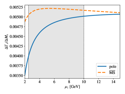
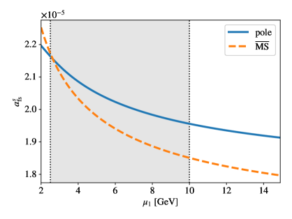
(a)	(b)

Figure 2: $\Delta\Gamma_{s}/\Delta M_{s}$ and $a^{s}_{\rm fs}$ as a function of $\mu_{1}$ for the $\overline{\rm MS}$ (dashed orange) and pole (solid blue) renormalization schemes. The gray area shows the range of $\mu_{1}$ used to obtain the renormalization scale uncertainties quoted in Eqs. (69) and (70).

 

The last three uncertainties in Eq. (69) are correlated between the two schemes. The scale dependence is plotted in Fig. 2(a) and leads to the asymmetric uncertainties quoted in Eq. (69). The difference between the central values found in the pole and $\overline{\rm MS}$ schemes is around 11%, i.e. of the expected size of an NNLO correction.

We proceed in a similar way for $a_{\rm fs}^{s}$. We use Eq. (2) and obtain

$$a_{\rm fs}^{s} = (2.07{}^{+0.10}_{-0.11}{}_{\rm scale}\pm 0.01_{B\tilde{B}_{S}}\pm 0.06_{1/m_{b}}\pm 0.06_{\textrm{input}})\times 10^{-5}\quad(\textrm{pole})\,,$$

$$a_{\rm fs}^{s} = (2.02{}^{{+0.15}}_{-0.17}{}_{\rm scale}\pm 0.01_{B\tilde{B}_{S}}\pm 0.05_{1/m_{b}}\pm 0.06_{\textrm{input}})\times 10^{-5}\quad(\overline{\textrm{MS}})\,.$$ (70)

In Fig. 2(b) we show the dependence on $\mu_{1}$ for the two renormalization schemes. Here the interval in the pole scheme is completely contained in the one from the $\overline{\rm MS}$ scheme.

The predictions in Eqs. (69) and (70) are consistent with those of Ref. [14], but the central values for $\Delta\Gamma_{s}/\Delta M_{s}$ in Eq. (69) are larger in both schemes. In Ref. [14] only partial NLO corrections to the $Q_{1,2}\times Q_{3-6}$ contribution and no $Q_{3-6}\times Q_{3-6}$ or NNLO $Q_{8}$ terms have been included. Inspecting the sources of the differences in detail, we find that almost 2/3 of these stem from the new contributions presented in Ref. [15] and this paper. The remainder is due to terms, which are formally of higher order in $\alpha_{s}$. Interestingly, the $\mu_{1}$ dependence of $\Delta\Gamma_{s}/\Delta M_{s}$ is much smaller in Eq. (69) compared to Ref. [14], while the situation is vice versa for $a_{\rm fs}^{s}$. We trace this feature back to the use of $\alpha_{s}(\mu_{1})$ versus $\alpha_{s}(\mu_{2})$ in certain NLO terms, both of which are allowed choices in the considered order. In view of this observation and the fact that the intervals from the scale uncertainty of $\Delta\Gamma_{s}/\Delta M_{s}$ in both schemes barely overlap, we conclude that the $\mu_{1}$ dependence is not always a good estimate of the size of the unknown higher-order corrections.

In a next step we can use the experimental result for $\Delta M_{s}$ [33],

$$\Delta M_{s}^{\rm exp} = 17.7656\pm 0.0057~{}\mbox{ps}^{-1}\,,$$ (71)

and obtain for $\Delta\Gamma_{s}$ in the two renormalization schemes

$$\Delta\Gamma_{s}^{\rm pole} = (0.083^{+0.005}_{-0.012}{}_{\rm scale}\pm 0.002_{B\tilde{B}_{S}}\pm 0.014_{1/m_{b}}\pm 0.001_{\textrm{input}})~{}\mbox{ps}^{-1}\,,$$

$$\Delta\Gamma_{s}^{\overline{\rm MS}} = (0.092^{+0.0002}_{{-0.003}}{}_{\rm scale}\pm 0.002_{B\tilde{B}_{S}}\pm 0.012_{1/m_{b}}\pm 0.001_{\textrm{input}})~{}\mbox{ps}^{-1}\,.$$ (72)

Comparing our prediction with the experimental value in Eq. (4) we see that both the “pole” and $\overline{\rm MS}$ results are consistent with the measured value, but the central value of the former is closer to the experimental result. One needs a better perturbative precision (which will bring the “pole” and $\overline{\rm MS}$ results closer to each other and reduce the scale uncertainty) and more precise lattice results for the matrix elements of the $1/m_{b}$-suppressed operators to quantify new-physics contributions to $\Delta\Gamma_{s}/\Delta M_{s}$.

The value for $\Delta\Gamma_{s}/\Delta M_{s}$ quoted in Eq. (69) also applies to $\Delta\Gamma_{d}/\Delta M_{d}$ for two reasons: First, while the CKM-suppressed contribution to $\Delta\Gamma_{d}/\Delta M_{d}$ is a priori expected to be relevant due to $|\lambda^{d}_{u}/\lambda^{d}_{t}|\gg|\lambda^{s}_{u}/\lambda^{s}_{t}|$, it merely contributes at the percent level because of a numerical cancellation in the sum of $uc$ and $uu$ contributions [11]. Second, the non-perturbative calculations of the $B_{s}$ and $B_{d}$ hadronic matrix elements agree well within their error bars. As a result the central values for $\Delta\Gamma_{d}/\Delta M_{d}$ and $\Delta\Gamma_{s}/\Delta M_{s}$ agree within a few percent (see e.g. [14]) and the difference is much smaller than the uncertainty in Eq. (69). We find

$$\Delta\Gamma_{d}^{\rm pole} \simeq \frac{\Delta\Gamma_{s}}{\Delta M_{s}}\Big{|}_{\rm pole}\Delta M_{d}^{\rm exp}$$

$$= ({0.00238}^{+0.00016}_{-0.00036}{}_{\rm scale}\pm 0.00006_{B\tilde{B}_{S}}\pm 0.00040_{1/m_{b}}\pm 0.00003_{\textrm{input}})~{}\mbox{ps}^{-1}\,,$$

$$\Delta\Gamma_{d}^{\overline{\rm MS}} \simeq \frac{\Delta\Gamma_{s}}{\Delta M_{s}}\Big{|}_{\rm\overline{\rm MS}}\Delta M_{d}^{\rm exp}$$ (73)

$$= (0.00264^{+0.00001}_{-0.00008}{}_{\rm scale}\pm 0.00006_{B\tilde{B}_{S}}\pm 0.00034_{1/m_{b}}\pm 0.00003_{\textrm{input}})~{}\mbox{ps}^{-1}\,.$$

where $\Delta M_{d}^{\rm exp}=(0.5065\pm 0.0019)\,\mbox{ps}^{-1}$ [2] has been used.

6 Conclusions

In this paper we have completed the calculation of the NLO contributions to the decay matrix element $\Gamma_{12}^{q}$ appearing in $B_{q}\!-\!\bar{B}{}_{q}\,$ mixing. These new contributions involve two-loop diagrams with two four-quark penguin operators. We have further calculated two-loop contributions with one or two copies of the chromomagnetic penguin operators, which belong to NNLO or N³LO, respectively. All results are obtained as an expansion to first order in $z=m_{c}^{2}/m_{b}^{2}$, except for the one-loop $Q_{8}\times Q_{8}$ contribution for which our result has the exact $z$-dependence. With our new results the theoretical uncertainties associated with the penguin sector are under full control and way below the experimental error of the width difference $\Delta\Gamma_{s}\simeq 2|\Gamma_{12}^{s}|$ in Eq. (4). We present updated predictions for $\Delta\Gamma_{s}$ and $\Delta\Gamma_{d}$ and the CP asymmetry in flavor-specific $B_{s}$ decays, $a^{s}_{\rm fs}$. For the width differences we find the predictions in the pole and $\overline{\rm MS}$ schemes to differ by 11%, which invigorates the need for a full NNLO calculation of the contributions from current-current operators.

We provide the newly obtained matching coefficients in a computer readable format with full dependence on the number of colors $N_{c}$. In the same way we present the renormalization matrix $Z_{ij}$ of the $\Delta B=2$ operators including the submatrices governing the mixing of evanescent operators with physical operators and among each other.

Appendix A Renormalization constants

In this Appendix we describe the computation of the renormalization constants required for the operator mixing in the $|\Delta B|=2$ theory and provide explicit results relevant for the two-loop calculations presented in the main part of this paper. Let us mention that all relevant renormalization constants for the $|\Delta B|=1$ theory can be found in Ref. [29].

For the computation of renormalization constants in the $\overline{\rm MS}$ scheme we can choose the external momenta and particle masses such, that the amplitude $b+\bar{s}\to\bar{b}+s$ is infra-red finite. This is possible since $\overline{\rm MS}$ renormalization constants do not depend on kinematic invariants and masses. In our case it is convenient to set all external momenta to zero and introduce a common mass for the strange and bottom quark. The gluon remains massless. This leads to one-loop vacuum integrals.

We work in a basis with physical operators $Q$, $\widetilde{Q}_{S}$ (c.f. Eq. (9)) and $R_{0}$ and the corresponding evanescent operators $E_{1}^{(1)},\ldots,E_{5}^{(1)}$ from Eq. (13). We have to introduce further evanescent operators, which contains the Dirac structures present in the $\Delta B=1$ amplitude. As can be seen from Tab. 1 the contribution $Q_{3-6}\times Q_{3-6}$ has the largest number of $\gamma$ matrices and requires that the evanescent operators $E_{i}^{(4)}$ (see Eq. (14)) are taken into account in the computation of the amplitude. The same evanescent operators are also needed for the computation of the renormalization constants. In analogy to the amplitude calculation, also for the renormalization constants the ${\cal O}(\epsilon)$ terms $e_{i,j}$ defined in Eq. (14) are only needed for $E_{i}^{(1)}$.

We can write the matrix of renormalization constants as a $20\times 20$ matrix which is naturally decomposed into four sub-matrices

$$Z_{\Delta B=2} = \left(\begin{array}[]{cc}Z_{QQ}&Z_{QE}\\ Z_{EQ}&Z_{EE}\end{array}\right)\,,$$ (76)

where $Z_{QQ}$, $Z_{QE}$, $Z_{EQ}$ and $Z_{EE}$ have the dimension $3\times 3$, $3\times 17$, $17\times 3$ and $17\times 17$, respectively. We define $Z_{\Delta B=2}$ via the renormalization of the coefficient functions as follows

$$\vec{C}^{\rm bare} = Z_{\Delta B=2}^{T}\vec{C}^{\rm ren}\,,$$ (77)

where $\vec{C}^{\rm bare}$ and $\vec{C}^{\rm ren}$ are 20-dimensional vectors of the bare and renormalized $|\Delta B|=2$ coefficient functions, respectively. The perturbative expansion of the sub-matrices is introduced as

$$Z_{QQ} = 1+\frac{\alpha_{s}}{4\pi}\frac{1}{\epsilon}Z_{QQ}^{(1,1)}\,,$$

$$Z_{QE} = \frac{\alpha_{s}}{4\pi}\frac{1}{\epsilon}Z_{QE}^{(1,1)}\,,$$

$$Z_{EE} = 1+\frac{\alpha_{s}}{4\pi}\frac{1}{\epsilon}Z_{EE}^{(1,1)}\,,$$

$$Z_{EQ} = \frac{\alpha_{s}}{4\pi}Z_{EQ}^{(1,0)}\,,$$ (78)

where the first superscript denotes the order in $\alpha_{s}$ and the second one the order in $1/\epsilon$. Note that at one-loop order the matrix $Z_{EQ}$ only contains finite contributions.

In order to determine the matrix elements of $Z_{\Delta B=2}$ we compute the amplitude $b+\bar{s}\to\bar{b}+s$ in the kinematics described above, take into account the field renormalization of the external quarks in the $\overline{\rm MS}$ scheme and require that the remaining poles in $\epsilon$, which are all of ultra-violet nature, are absorbed by the operator mixing via $Z_{\Delta B=2}$. This condition fixes all matrix elements but the ones in $Z_{EQ}$. The latter are fixed by the requirement that the contributions of evanescent operators vanish in $D=4$ dimensions [39, 20]. Note that to our order we do not have to renormalize the common strange and bottom quark mass.

An important check of our calculation is the locality of the extracted renormalization constants. Furthermore, we perform the calculation for general QCD gauge parameter and observe that the matrix $Z_{\Delta B=2}$ is independent of $\xi$.

In the following we present explicit results for the one-loop corrections to $Z_{QQ}$, $Z_{QE}$ and $Z_{EE}$. For $N_{c}=3$ we have

$$Z_{QQ}^{(1,1)} =\left(\begin{array}[]{ccc}2&0&0\\ -\frac{4}{3}&\frac{8}{3}&\frac{8}{3}\\ 2&8&-2\\ \end{array}\right)\,,$$ (82)

$$Z_{QE}^{(1,1)} =\left(\begin{array}[]{ccccccccccccccccc}3&\frac{1}{2}&-\frac{1}{6}&0&0&0&0&0&0&0&0&0&0&0&0&0&0\\ 0&0&0&-\frac{7}{12}&-\frac{1}{4}&0&0&0&0&0&0&0&0&0&0&0&0\\ \frac{3}{2}&\frac{1}{4}&-\frac{1}{12}&-\frac{13}{12}&-\frac{1}{12}&0&0&0&0&0&0&0&0&0&0&0&0\\ \end{array}\right)\,,$$ (86)

where the entries “$\ast$” are not needed for our calculation.

The (finite) matrix $Z_{EQ}^{(1,0)}$ depends on the ${\cal O}(\epsilon)$ terms of the evanescent operators, $e^{(i)}_{j}$ and $e^{(i)}_{j,k}$. It is given by

$$Z_{EQ}^{(1,0)} = \begin{pmatrix}Z_{EQ,1}^{(1,0)}&Z_{EQ,2}^{(1,0)}&Z_{EQ,3}^{(1,0)}\end{pmatrix}\,,$$ (88)

where

$$Z_{EQ,1}^{(1,0)} =\left(\begin{array}[]{c}0\\ \frac{7}{12}e_{1}^{(2)}+\frac{1}{4}e_{2}^{(2)}+\frac{464}{3}\\ \frac{1}{2}e_{1}^{(2)}-\frac{1}{6}e_{2}^{(2)}-\frac{16}{3}\\ \frac{1}{8}e_{3,2}^{(2)}+\frac{7}{24}e_{4,2}^{(2)}+84\\ -\frac{1}{12}e_{3,2}^{(2)}+\frac{1}{4}e_{4,2}^{(2)}+44\\ \frac{35}{3}e_{1}^{(2)}+\frac{7}{12}e_{1}^{(3)}-9e_{2}^{\ (2)}+\frac{1}{4}e_{2}^{(3)}+\frac{17920}{3}\\ 3e_{1}^{(2)}+\frac{1}{2}e_{1}^{(3)}-\frac{73}{3}e_{2}^{\ (2)}-\frac{1}{6}e_{2}^{(3)}-\frac{14336}{3}\\ \frac{4}{3}e_{3,1}^{(2)}+\frac{4}{3}e_{3,2}^{(2)}+e_{4,2}^{\ (2)}+\frac{1}{12}e_{3,2}^{(3)}-\frac{1}{4}e_{4,2}^{(3)}+64\\ 2e_{3,2}^{(2)}-\frac{1}{8}e_{3,2}^{(3)}+\frac{4}{3}e_{4,1}^{\ (2)}-\frac{5}{3}e_{4,2}^{(2)}-\frac{7}{24}e_{4,2}^{(3)}-1728\\ -672e_{1}^{(2)}+\frac{179}{3}e_{1}^{(3)}+\frac{7}{12}e_{1}^{(4)}+224\ e_{2}^{(2)}-25e_{2}^{(3)}+\frac{1}{4}e_{2}^{(4)}+\frac{901120}{3}\\ -224e_{1}^{(2)}+19e_{1}^{(3)}+\frac{1}{2}e_{1}^{(4)}+672e_{2}^{(2)}-\ \frac{217}{3}e_{2}^{(3)}-\frac{1}{6}e_{2}^{(4)}-\frac{843776}{3}\\ -360e_{3,2}^{(2)}+\frac{58}{3}e_{3,2}^{(3)}+\frac{1}{12}\ e_{3,2}^{(4)}+120e_{4,2}^{(2)}+\frac{4}{3}e_{3,1}^{(3)}-5\ e_{4,2}^{(3)}-\frac{1}{4}e_{4,2}^{(4)}+24064\\ -120e_{3,2}^{(2)}+8e_{3,2}^{(3)}-\frac{1}{8}e_{3,2}^{(4)}+360\ e_{4,2}^{(2)}+\frac{4}{3}e_{4,1}^{(3)}-\frac{59}{3}e_{4,2}^{\ (3)}-\frac{7}{24}e_{4,2}^{(4)}-44544\\ \ast\\ \ast\\ \ast\\ \ast\\ \end{array}\right),$$ (106)

$$Z_{EQ,2}^{(1,0)} =\left(\begin{array}[]{c}0\\ 0\\ 0\\ -\frac{1}{4}e_{3,1}^{(2)}+\frac{1}{4}e_{3,2}^{(2)}-\frac{7}{12}e_{4,1}^{(2)}+\frac{7}{12}e_{4,2}^{(2)}+32\\ \frac{1}{6}e_{3,1}^{(2)}-\frac{1}{6}e_{3,2}^{(2)}-\frac{1}{2}e_{4,1}^{(2)}+\frac{1}{2}e_{4,2}^{(2)}+32\\ 0\\ 0\\ -10e_{3,1}^{(2)}-\frac{1}{6}e_{3,1}^{(3)}+2e_{3,2}^{(2)}-2e_{4,1}^{(2)}+2e_{4,2}^{(2)}+\frac{1}{6}e_{3,2}^{(3)}+\frac{1}{2}e_{4,1}^{(3)}-\frac{1}{2}e_{4,2}^{(3)}-1536\\ -4e_{3,1}^{(2)}+\frac{1}{4}e_{3,1}^{(3)}+4e_{3,2}^{(2)}-4e_{4,1}^{(2)}-4e_{4,2}^{(2)}-\frac{1}{4}e_{3,2}^{(3)}+\frac{7}{12}e_{4,1}^{(3)}-\frac{7}{12}e_{4,2}^{(3)}-1536\\ 0\\ 0\\ 720e_{3,1}^{(2)}-46e_{3,1}^{(3)}-\frac{1}{6}e_{3,1}^{(4)}-720e_{3,2}^{(2)}-240e_{4,1}^{(2)}+240e_{4,2}^{(2)}+38e_{3,2}^{(3)}+10e_{4,1}^{(3)}-10e_{4,2}^{(3)}+\frac{1}{6}e_{3,2}^{(4)}+\frac{1}{2}e_{4,1}^{(4)}-\frac{1}{2}e_{4,2}^{(4)}-12288\\ 240e_{3,1}^{(2)}-16e_{3,1}^{(3)}+\frac{1}{4}e_{3,1}^{(4)}-240e_{3,2}^{(2)}-720e_{4,1}^{(2)}+720e_{4,2}^{(2)}+16e_{3,2}^{(3)}+32e_{4,1}^{(3)}-40e_{4,2}^{(3)}-\frac{1}{4}e_{3,2}^{(4)}+\frac{7}{12}e_{4,1}^{(4)}-\frac{7}{12}e_{4,2}^{(4)}-12288\\ \ast\\ \ast\\ \ast\\ \ast\\ \end{array}\right),$$ (124)

$$Z_{EQ,3}^{(1,0)} =\left(\begin{array}[]{c}0\\ 0\\ 0\\ -\frac{1}{4}e_{3,2}^{(2)}-\frac{7}{12}e_{4,2}^{(2)}-168\\ \frac{1}{6}e_{3,2}^{(2)}-\frac{1}{2}e_{4,2}^{(2)}-88\\ 0\\ 0\\ -\frac{8}{3}e_{3,1}^{(2)}-\frac{8}{3}e_{3,2}^{(2)}-2e_{4,2}^{(2)}-\frac{1}{6}e_{3,2}^{(3)}+\frac{1}{2}e_{4,2}^{(3)}-128\\ -4e_{3,2}^{(2)}+\frac{1}{4}e_{3,2}^{(3)}-\frac{8}{3}e_{4,1}^{(2)}+\frac{10}{3}e_{4,2}^{(2)}+\frac{7}{12}e_{4,2}^{(3)}+3456\\ 0\\ 0\\ 720e_{3,2}^{(2)}-\frac{116}{3}e_{3,2}^{(3)}-\frac{1}{6}e_{3,2}^{(4)}-240e_{4,2}^{(2)}-\frac{8}{3}e_{3,1}^{(3)}+10e_{4,2}^{(3)}+\frac{1}{2}e_{4,2}^{(4)}-48128\\ 240e_{3,2}^{(2)}-16e_{3,2}^{(3)}+\frac{1}{4}e_{3,2}^{(4)}-720e_{4,2}^{(2)}-\frac{8}{3}e_{4,1}^{(3)}+\frac{118}{3}e_{4,2}^{(3)}+\frac{7}{12}e_{4,2}^{(4)}+89088\\ \ast\\ \ast\\ \ast\\ \ast\\ \end{array}\right).$$ (142)

References

- [1] R. Aaij et al. [LHCb], Precise determination of the - oscillation frequency, [arXiv:2104.04421 [hep-ex]].
-
[2]
Heavy Flavor Averaging Group (HFLAV),
https://hflav-eos.web.cern.ch/hflav-eos/osc/PDG_2020/\# DMS - [3] R. Aaij et al. [LHCb], Neutral B-meson mixing from full lattice QCD at the physical point, Eur. Phys. J. C 79 (2019) no.8, 706 [erratum: Eur. Phys. J. C 80 (2020) no.7, 601] [arXiv:1906.08356 [hep-ex]].
- [4] A. M. Sirunyan et al. [CMS], Measurement of the -violating phase in the B J(1020) K+K- channel in proton-proton collisions at 13 TeV, Phys. Lett. B 816 (2021), 136188, doi:10.1016/j.physletb.2021.136188 [arXiv:2007.02434 [hep-ex]].
- [5] G. Aad et al. [ATLAS], Measurement of the -violating phase in decays in ATLAS at 13 TeV, Eur. Phys. J. C 81 (2021) no.4, 342 doi:10.1140/epjc/s10052-021-09011-0 [arXiv:2001.07115 [hep-ex]].
- [6] T. Aaltonen et al. [CDF], Measurement of the Bottom-Strange Meson Mixing Phase in the Full CDF Data Set, Phys. Rev. Lett. 109 (2012), 171802, doi:10.1103/PhysRevLett.109.171802 [arXiv:1208.2967 [hep-ex]].
- [7] V. M. Abazov et al. [D0], Measurement of the CP-violating phase using the flavor-tagged decay in 8 fb-1 of collisions, Phys. Rev. D 85 (2012), 032006, doi:10.1103/PhysRevD.85.032006 [arXiv:1109.3166 [hep-ex]].
- [8] R. J. Dowdall, C. T. H. Davies, R. R. Horgan, G. P. Lepage, C. J. Monahan, J. Shigemitsu and M. Wingate, Neutral B-meson mixing from full lattice QCD at the physical point, Phys. Rev. D 100 (2019) no.9, 094508 [arXiv:1907.01025 [hep-lat]].
- [9] M. Beneke, G. Buchalla, C. Greub, A. Lenz and U. Nierste, Next-to-Leading Order QCD Corrections to the Lifetime Difference of Mesons, Phys. Lett. B 459 (1999), 631-640 [arXiv:hep-ph/9808385 [hep-ph]].
- [10] M. Ciuchini, E. Franco, V. Lubicz, F. Mescia and C. Tarantino, Lifetime Differences and CP Violation Parameters of Neutral B Mesons at the Next-to-Leading Order in QCD, JHEP 08 (2003), 031 [arXiv:hep-ph/0308029 [hep-ph]].
- [11] M. Beneke, G. Buchalla, A. Lenz and U. Nierste, CP asymmetry in flavour-specific B decays beyond leading logarithms, Phys. Lett. B 576 (2003), 173-183 [arXiv:hep-ph/0307344 [hep-ph]].
- [12] A. Lenz and U. Nierste, Theoretical update of – mixing, JHEP 06 (2007), 072 [arXiv:hep-ph/0612167 [hep-ph]].
- [13] H. M. Asatrian, A. Hovhannisyan, U. Nierste and A. Yeghiazaryan, Towards next-to-next-to-leading-log accuracy for the width difference in the –: fermionic contributions to order and , JHEP 10 (2017), 191 [arXiv:1709.02160 [hep-ph]].
- [14] H. M. Asatrian, H. H. Asatryan, A. Hovhannisyan, U. Nierste, S. Tumasyan and A. Yeghiazaryan, Penguin contribution to the width difference and asymmetry in - mixing at order , Phys. Rev. D 102 (2020) no.3, 033007 doi:10.1103/PhysRevD.102.033007 [arXiv:2006.13227 [hep-ph]].
- [15] M. Gerlach, U. Nierste, V. Shtabovenko and M. Steinhauser, Two-loop QCD penguin contribution to the width difference in – mixing,” JHEP 07 (2021), 043 doi:10.1007/JHEP07(2021)043 [arXiv:2106.05979 [hep-ph]].
- [16] M. Beneke, G. Buchalla and I. Dunietz, Width Difference in the – System, Phys. Rev. D 54 (1996), 4419-4431 [erratum: Phys. Rev. D 83 (2011), 119902] doi:10.1103/PhysRevD.54.4419 [arXiv:hep-ph/9605259 [hep-ph]].
- [17] C. T. H. Davies et al. [HPQCD], Lattice QCD matrix elements for the – width difference beyond leading order, Phys. Rev. Lett. 124 (2020) no.8, 082001 [arXiv:1910.00970 [hep-lat]].
- [18] K. G. Chetyrkin, M. Misiak and M. Munz, nonleptonic effective Hamiltonian in a simpler scheme, Nucl. Phys. B 520 (1998), 279-297 [arXiv:hep-ph/9711280 [hep-ph]].
- [19] M. Gorbahn, S. Jager, U. Nierste and S. Trine, The supersymmetric Higgs sector and – mixing for large , Phys. Rev. D 84 (2011), 034030 doi:10.1103/PhysRevD.84.034030 [arXiv:0901.2065 [hep-ph]].
- [20] S. Herrlich and U. Nierste, Evanescent operators, scheme dependences and double insertions, Nucl. Phys. B 455 (1995), 39-58 doi:10.1016/0550-3213(95)00474-7 [arXiv:hep-ph/9412375 [hep-ph]].
- [21] R. Mertig, M. Bohm and A. Denner, FEYN CALC: Computer algebraic calculation of Feynman amplitudes, Comput. Phys. Commun. 64 (1991) 345-359 doi:10.1016/0010-4655(91)90130-D.
- [22] V. Shtabovenko, R. Mertig and F. Orellana, New Developments in FeynCalc 9.0, Comput. Phys. Commun. 207 (2016), 432-444 doi:10.1016/j.cpc.2016.06.008 [arXiv:1601.01167 [hep-ph]].
- [23] V. Shtabovenko, R. Mertig and F. Orellana, FeynCalc 9.3: New features and improvements, Comput. Phys. Commun. 256 (2020), 107478 doi:10.1016/j.cpc.2020.107478 [arXiv:2001.04407 [hep-ph]].
-
[24]
R. H. Lewis, Computer Algebra System Fermat,
http://www.bway.net/~lewis. - [25] J. Kuipers, T. Ueda, J. A. M. Vermaseren and J. Vollinga, FORM version 4.0, Comput. Phys. Commun. 184 (2013), 1453-1467 [arXiv:1203.6543 [cs.SC]].
- [26] A. V. Smirnov and F. S. Chuharev, FIRE6: Feynman Integral REduction with Modular Arithmetic, Comput. Phys. Commun. 247 (2020), 106877 doi:10.1016/j.cpc.2019.106877 [arXiv:1901.07808 [hep-ph]].
- [27] R. N. Lee, Presenting LiteRed: a tool for the Loop InTEgrals REDuction, [arXiv:1212.2685 [hep-ph]].
- [28] R. N. Lee, LiteRed 1.4: a powerful tool for reduction of multiloop integrals, J. Phys. Conf. Ser. 523 (2014), 012059 doi:10.1088/1742-6596/523/1/012059 [arXiv:1310.1145 [hep-ph]].
- [29] P. Gambino, M. Gorbahn and U. Haisch, Anomalous dimension matrix for radiative and rare semileptonic B decays up to three loops, Nucl. Phys. B 673 (2003), 238-262 doi:10.1016/j.nuclphysb.2003.09.024 [arXiv:hep-ph/0306079 [hep-ph]].
- [30] M. Ciuchini, E. Franco, V. Lubicz and F. Mescia, Next-to-leading order QCD corrections to spectator effects in lifetimes of beauty hadrons, Nucl. Phys. B 625 (2002), 211-238 doi:10.1016/S0550-3213(02)00006-8 [arXiv:hep-ph/0110375 [hep-ph]].
-
[31]
https://www.ttp.kit.edu/preprints/2022/ttp22-012/. - [32] H. E. Logan and U. Nierste, in a two Higgs doublet model, Nucl. Phys. B 586 (2000), 39-55 doi:10.1016/S0550-3213(00)00417-X [arXiv:hep-ph/0004139 [hep-ph]].
- [33] P. A. Zyla et al. [Particle Data Group], PTEP 2020 (2020) no.8, 083C01.
- [34] K. G. Chetyrkin, J. H. Kuhn, A. Maier, P. Maierhofer, P. Marquard, M. Steinhauser and C. Sturm, Addendum to “Charm and bottom quark masses: An update”, Phys. Rev. D 96 (2017) no.11, 116007 doi:10.1103/PhysRevD.96.116007 [arXiv:1710.04249 [hep-ph]].
- [35] A. Bazavov, C. Bernard, N. Brown, C. Detar, A. X. El-Khadra, E. Gámiz, S. Gottlieb, U. M. Heller, J. Komijani and A. S. Kronfeld, et al. - and -meson leptonic decay constants from four-flavor lattice QCD, Phys. Rev. D 98 (2018) no.7, 074512 doi:10.1103/PhysRevD.98.074512 [arXiv:1712.09262 [hep-lat]].
- [36] B. Chakraborty, C. T. H. Davies, B. Galloway, P. Knecht, J. Koponen, G. C. Donald, R. J. Dowdall, G. P. Lepage and C. McNeile, High-precision quark masses and QCD coupling from lattice QCD, Phys. Rev. D 91 (2015) no.5, 054508 doi:10.1103/PhysRevD.91.054508 [arXiv:1408.4169 [hep-lat]].
- [37] M. Beneke, G. Buchalla, C. Greub, A. Lenz and U. Nierste, The Lifetime Difference Beyond Leading Logarithms, Nucl. Phys. B 639 (2002), 389-407 doi:10.1016/S0550-3213(02)00561-8 [arXiv:hep-ph/0202106 [hep-ph]].
- [38] A. J. Buras, M. Jamin and P. H. Weisz, Leading and Next-to-leading QCD Corrections to Parameter and – Mixing in the Presence of a Heavy Top Quark, Nucl. Phys. B 347 (1990), 491-536 doi:10.1016/0550-3213(90)90373-L.
- [39] A. J. Buras and P. H. Weisz, QCD Nonleading Corrections to Weak Decays in Dimensional Regularization and ’t Hooft-Veltman Schemes, Nucl. Phys. B 333 (1990), 66-99 doi:10.1016/0550-3213(90)90223-Z.