Conformally curved initial data for charged, spinning black hole binaries on arbitrary orbits

Abstract

We present a method to construct conformally curved initial data for charged black hole binaries with spin on arbitrary orbits. We generalize the superposed Kerr-Schild, extended conformal thin sandwich construction from [Lovelace et al., Phys. Rev. D 78, 084017 (2008)] to use Kerr-Newman metrics for the superposed black holes and to solve the electromagnetic constraint equations. We implement the construction in the pseudospectral code SGRID. The code thus provides a complementary and completely independent excision-based construction, compared to the existing charged black hole initial data constructed using the puncture method [Bozzola and Paschalidis, Phys. Rev. D 99, 104044 (2019)]. It also provides an independent implementation (with some small changes) of the Lovelace et al. vacuum construction. We construct initial data for different configurations of orbiting binaries, e.g., with black holes that are highly charged or rapidly spinning (90 and 80 percent of the extremal values, respectively, for this initial test, though the code should be able to produce data with even higher values of these parameters using higher resolutions), as well as for generic spinning, charged black holes. We carry out exploratory evolutions with the finite difference, moving punctures codes BAM (in the vacuum case) and HAD (for head-on collisions including charge), filling inside the excision surfaces. In the charged case, evolutions of these initial data provide a proxy for binary black hole waveforms in modified theories of gravity. Moreover, the generalization of the construction to Einstein-Maxwell-dilaton theory should be straightforward.

I Introduction

Gravitational wave (GW) observations of compact binary mergers, primarily binary black holes (e.g., Abbott et al. (2019a, 2021a, 2021b)), have made it possible to test general relativity (GR) in the strong-field, high velocity regime where GR is most likely to break down (see Abbott et al. (2019b, 2021c, 2021d) for results of such tests carried out by the LIGO-Virgo collaboration). However, these tests are all null tests of one sort or another, and one would ideally want to compare the predictions of GR for the coalescence of compact binaries with the predictions of a suite of well-motivated alternative theories (in particular, Chua and Vallisneri (2020) discusses some of the problems encountered with certain null tests). To carry out such comparisons, one needs to construct high-accuracy waveform models in alternative theories, just as have been constructed in GR. At present, constraints on alternative theories using binary black hole observations have been restricted to using model waveforms constructed with only low-order post-Newtonian (PN) calculations in the alternative theories Perkins et al. (2021); Wang et al. (2021).

Numerical relativity simulations of the late inspiral and merger in alternative theories will be a key ingredient in constructing such waveform models, just as in GR. However, such simulations come with several challenges. Many of these modified theories either do not have a known well-posed initial value formulation (making them unsuitable for numerical evolution) or lack a construction of constraint-satisfying initial data for compact binaries. While significant progress has been made towards finding a well-posed formulation for Einstein-scalar-Gauss-Bonnet, Lovelock, and Horndeski theories at weak coupling Kovács and Reall (2020a, b) and their subsequent numerical evolution East and Ripley (2021a, b); Figueras and França (2021), most approaches to simulating binary black holes in modified theories of gravity depend on an order reduction method Okounkova et al. (2020, 2019); Okounkova (2020); Witek et al. (2019); Silva et al. (2021). Such approaches compute the effects of modified theories as perturbations to the GR solution, which leads to a secular drift between the true solution and the perturbative solution Okounkova et al. (2020); Okounkova (2020), though there are proposals for methods to remove this drift Gálvez Ghersi and Stein (2021). There are also approaches that modify the equations to make the theories well-posed Cayuso and Lehner (2020), but not yet any evolutions of binary black holes with such approaches.

For theories that do have a known well-posed initial value formulation, evolutions of binary black hole mergers have been carried out using approximate initial data. Examples include a study Hirschmann et al. (2018) in Einstein-Maxwell-dilaton theory Gibbons and Maeda (1988) and evolutions in scalar-tensor theories of gravity Berti et al. (2013); Healy et al. (2012) where, in the absence of externally imposed scalar field dynamics, binary black holes in scalar-tensor theory have the same dynamics as those in vacuum GR.

Here we consider charged binary black holes in Einstein-Maxwell theory. This provides a well-posed framework that mimics some of the features of binary black hole mergers in modified theories. Additionally, various modified theories besides Einstein-Maxwell-dilaton theory also contain vector fields with a Maxwell-like kinetic term (see, e.g., Will (2014)), so this is a first step to performing simulations in those theories. The specific features of Einstein-Maxwell theory that mimic some of the effects seen in modified theories are modified or additional PN terms in the dynamics of the binary (see, e.g., Khalil et al. (2018)) and differences in the spectrum of quasinormal modes for the final black hole (see, e.g., Dias et al. (2015, 2021); Carullo et al. (2021)). Both of these effects are directly encoded in the binary’s GW signal. In particular, charged binary black holes with unequal charge-to-mass ratios emit dipole radiation (see, e.g., Khalil et al. (2018)), a common feature in several modified theories of gravity, e.g., scalar Gauss-Bonnet (sGB) gravity Shiralilou et al. (2022) and scalar-tensor theories of gravity Sennett et al. (2016). Binary black holes emit dipole radiation due to a charge in sGB gravity, as well, though there it is a scalar charge, as opposed to the $\rm{U}(1)$ charge we consider here. Binary black holes in scalar-tensor theories do not emit dipole radiation, but systems with matter will in general emit scalar dipole radiation in those theories. Nevertheless, the leading PN effect of the dipole radiation on the binary’s dynamics will have the same frequency dependence in all cases, viz., a $-1$PN order contribution to the orbital phasing and thus to the phase of the GW signal (in the case where the dipole radiation can be treated as a perturbation to the dominant quadrupole radiation—see, e.g., Khalil et al. (2018)).

From an observational perspective, the LIGO-Virgo analyses (e.g., Abbott et al. (2019b, 2021c, 2021d)) currently test for the presence of such an additional $-1$PN term in the phase. In the absence of dipole radiation (which is the case for charged binary black holes with equal charge-to-mass ratio and the same sign of charge) the deviations from vacuum GR will only occur at $1\text{PN}$ order and above (since the $0\text{PN}$ modifications are degenerate with a rescaling of the binary’s masses, as discussed in, e.g., Cardoso et al. (2016)). This is similar to some modified theories, e.g., dynamical Chern-Simons theory, where the deviations from GR start at $2\text{PN}$ Yagi et al. (2012). Many of the other LIGO-Virgo tests of general relativity check (explicitly or implicitly) for such deviations in higher-order PN coefficients. Additionally, a recent analysis Carullo et al. (2021) checks for the presence of charge in the ringdown waveforms, but finds that one can only place very weak constraints using the ringdown phase alone due to correlations between the charge and spin parameters.

Charged binary black hole waveforms, therefore, provide a proxy for BBH waveforms from modified theories of GR that would allow us to test the sensitivity of current LIGO-Virgo tests of GR to completely consistent, parameterized deviations from GR (see Johnson-McDaniel et al. (2022) for an initial study using phenomenological waveforms). Since the charge can be varied freely up to the extremal limit, this allows for significant deviations from vacuum GR. Further, one can use the waveforms from numerical simulations of charged binary black holes to create a waveform model that one can use to analyze gravitational wave data. Such a waveform model would likely also have significant input from PN calculations Khalil et al. (2018); Julié (2018) and black hole perturbation theory computations of quasinormal modes Dias et al. (2015, 2021); Carullo et al. (2021), and possibly also from black hole perturbation theory/self-force calculations of waveforms in the extreme mass-ratio limit (see Zhu and Osburn (2018); Burton and Osburn (2020); Torres and Dolan (2020) for work in this direction involving charge). Such a model would allow one to constrain the charges of observed black holes. Such an analysis has already been carried out for low-mass, inspiral-dominated signals in Gupta et al. (2021) using a simple waveform model created by combining a vacuum GR model with the known, still relatively low-order PN contributions from the charges from Khalil et al. (2018). There is also a study of GW150914 using numerical relativity waveforms of charged binary black holes and simple data analysis arguments in Bozzola and Paschalidis (2021a) (see also further data analysis calculations with these waveforms in Bozzola and Paschalidis (2021b)).

A full waveform model tuned to numerical relativity simulations would also allow one to constrain the charges of high-mass binaries, as well as firming up the constraints obtained with the simple waveform model presented in Gupta et al. (2021). While astrophysical black holes are expected to have negligible electric charges (as reviewed in Cardoso et al. (2016)), they could have nonnegligible magnetic charges if magnetic monopoles exist (as discussed in Liebling and Palenzuela (2016); Preskill (1984)). Additionally, black holes could attain a significant charge in the scenario where the black holes are charged under a dark electromagnetic field, e.g., the minicharged dark matter scenario considered in Cardoso et al. (2016). As a first step towards constructing such waveform models, we construct initial data for spinning, charged binary black holes in orbit. Numerical relativity simulations of charged binary black hole mergers also provide the mapping from the initial masses, spins, and charges to the final mass and spin, and better knowledge of this mapping, particularly for close-to-extreme charges, will improve the modeling of possible gamma-ray backgrounds from mergers of charged primordial black holes Kritos and Silk (2021).

Several previous studies have investigated the dynamics of charged black holes in full numerical relativity. Zilhão et al. Zilhao et al. (2012); Zilhão et al. (2014) performed simulations of head-on collisions of nonspinning charged black holes from rest, using either analytic equal charge-to-mass ratio initial data or a simple numerical initial data construction to obtain opposite charge-to-mass ratios. Liebling et al. Liebling and Palenzuela (2016) carried out evolutions for weakly charged (electric and magnetic) black holes on quasicircular orbits starting from approximate initial data. Most notably, Bozzola and Paschalidis Bozzola and Paschalidis (2019) constructed conformally flat, puncture initial data for multiple charged black holes with linear and angular momenta using the conformal transverse traceless approach, and subsequently evolved a set of nonspinning binary black holes with small to moderate charges on quasicircular orbits in Bozzola and Paschalidis (2021a, b) and, more recently, head-on collisions of boosted, charged black holes in Bozzola (2022).

We take a different approach to solving for charged binary black hole initial data. Specifically, we construct conformally curved excision initial data by extending the approach developed by Lovelace et al. in Lovelace et al. (2008) to include charge. The approach is based on the Extended Conformal Thin-Sandwich formalism York (1999); Pfeiffer and York (2003) and uses the superposition of two boosted Kerr black holes in Kerr-Schild coordinates (weighted by attenuation functions) for the conformal metric. Compared to the conformal transverse traceless construction, this approach has several advantages (at least in the uncharged case). For example it allows for higher spins Lovelace et al. (2008), less junk radiation Lovelace (2009), and better control over the physics through the boundary conditions at the excision surfaces. For our case, we replace the Kerr black holes by Kerr-Newman black holes and solve for the final electric field by solving for a correction to the superposed electric field (given by a scalar potential) to satisfy the divergence constraint. We use a simple boundary condition for the scalar potential on the excision surfaces that allows us to fix the charges of the black holes. We compute the magnetic field from the superposed vector potentials so that it satisfies the divergence constraint by construction.

In this paper, we generate excision based initial data for both highly charged and highly spinning binaries using the pseudospectral initial data solver SGRID Tichy (2009); Dietrich et al. (2015), and perform exploratory evolutions of the initial data in some cases with both the BAM Brügmann et al. (2008) and HAD Liebling et al. (2020) evolution codes. Both of these codes use finite differences and moving punctures for evolution, but they use different algorithms to fill inside the excision surfaces, and only HAD can evolve the charged case.

In Sec. II, we first review the construction from Lovelace et al. (2008) and then give its extension to the charged case. In Sec. III, we discuss the details of our numerical implementation. We then show examples of our initial data construction and exploratory evolutions using BAM and HAD in Sec. IV. We conclude in Sec. V. In Appendix A, we give expressions for a Kerr-Newman black hole in Kerr-Schild form, while in Appendices B and C, we give details of the black hole filling algorithms used in BAM and HAD, respectively. We use lowercase Latin letters to denote spatial indices and Greek letters for spacetime indices. We reserve the index $A$ to label the black holes. Finally, we use geometric units $(G=c=1)$ and Gaussian units for the electromagnetic field throughout the paper.

II Initial Data Formalism

To compute constraint satisfying initial data on a Cauchy hypersurface, one needs to solve the Hamiltonian and momentum constraints for the geometry and the electomagnetic constraint equations. With standard decompositions, these constraints constitute a set of coupled, nonlinear, second order differential equations for a given set of freely specifiable variables, and this set has to be supplemented with appropriate boundary conditions; see, e.g., Baumgarte and Shapiro (2003) for an introduction to the gravitational constraint equations. There are several approaches to solving this problem, each with a different decomposition of the gravitational constraint equations and a corresponding unique group of freely specifiable variables (see, e.g., Cook (2000); Tichy (2017) for reviews). Different decompositions can result in different initial data, e.g., with different amounts of junk radiation Cook (2000); Alcubierre (2008) that could lead to different physical parameters of the binary. We now review one such decomposition, the Extended Conformal Thin Sandwich formalism, which forms the basis of our initial data construction.

II.1 The Extended Conformal Thin Sandwich Formalism

The Extended Conformal Thin Sandwich (XCTS) formalism York (1999); Pfeiffer and York (2003) is an alternative approach to the transverse-traceless construction Bowen and York (1980) for calculating initial data. In contrast to the transverse-traceless construction, it allows for some degree of control over the time evolution of the initial data. As is standard, this construction begins by splitting the spatial metric $\gamma_{ij}$ into a conformal factor $\psi$ and the conformally related metric $\tilde{\gamma}_{ij}$, and then splitting the extrinsic curvature $K_{ij}$ into its trace $K$ and a traceless part $A_{ij}$, giving

$$\gamma_{ij} ={}\psi^{4}\tilde{\gamma}_{ij},$$ (1a)

$$K_{ij} ={}A_{ij}+\dfrac{1}{3}\gamma_{ij}K.$$ (1b)

In the XCTS formalism, we are allowed to freely specify $\{\tilde{\gamma}_{ij},K\}$ together with their time derivatives $\{\tilde{u}_{ij},\partial_{t}K\}$. We then solve for $\{\gamma_{ij},K_{ij}\}$ in terms of $\psi$, the shift vector $\beta_{i}$, and the lapse $\alpha$ multiplied by the conformal factor ($\alpha\psi$), respectively.

II.1.1 XCTS equations

For a given choice of freely specifiable variables, the Hamiltonian and momentum constraint equations decompose into a set of coupled elliptic equations for $\psi,\alpha\psi$, and $\beta_{i}$ given by

$$\tilde{\nabla}_{j}\tilde{\nabla}^{j}\psi-\dfrac{1}{8}\tilde{R}\psi-\dfrac{1}{12}K^{2}\psi^{5}+\dfrac{1}{8}\psi^{-7}\tilde{A}^{ij}\tilde{A}_{ij} =-2\pi\psi^{5}\rho,$$ (2a)

$$\tilde{\nabla}_{j}\left[\dfrac{\psi^{7}}{2(\alpha\psi)}\left(\tilde{L}\beta\right)^{ij}\right]-\dfrac{2}{3}\psi^{6}\tilde{\nabla}^{i}K-\tilde{\nabla}_{j}\left[\dfrac{\psi^{7}}{2(\alpha\psi)}\tilde{u}^{ij}\right] =8\pi\psi^{10}J^{i},$$ (2b)

$$\tilde{\nabla}_{j}\tilde{\nabla}^{j}(\alpha\psi)-(\alpha\psi)\left[\dfrac{\tilde{R}}{8}+\dfrac{5}{12}K^{2}\psi^{4}+\dfrac{7}{8}\psi^{-8}\tilde{A}^{ij}\tilde{A}_{ij}\right]+\psi^{5}(\partial_{t}K-\beta^{k}\partial_{k}K) =(\alpha\psi)\left[2\pi\psi^{4}(\rho+2\sigma)\right],$$ (2c)

where

$$(\tilde{L}\beta)_{ij}:=\tilde{\nabla}_{i}\beta_{j}+\tilde{\nabla}_{j}\beta_{i}-\dfrac{2}{3}\tilde{\gamma}_{ij}\tilde{\nabla}_{k}\beta^{k},$$ (3a)

$$\tilde{A}^{ij}=\psi^{10}A^{ij}=\dfrac{\psi^{7}}{2(\alpha\psi)}\left[(\tilde{L}\beta)^{ij}-\tilde{u}^{ij}\right].$$ (3b)

In these equations, the terms decorated with a tilde are associated with the conformal metric. Thus, $\tilde{\nabla}_{j}$ and $\tilde{R}$ are the covariant derivative and Ricci scalar associated with $\tilde{\gamma}_{ij}$, respectively. We also have electric ($E_{i}$) and magnetic ($B_{i}$) fields due to the presence of charged black holes, so the expressions for energy density $\rho$, the momentum density $J^{i}$, and the trace of the stress tensor as measured by an Eulerian observer $\sigma$ are given by Alcubierre et al. (2009)

$$\rho={} \dfrac{1}{8\pi}\left(E^{i}E_{i}+B^{i}B_{i}\right)=\sigma,$$ (4a)

$$J^{i}={} \dfrac{1}{4\pi}(\mathbf{E}\times\mathbf{B})^{i},$$ (4b)

where

$$(\mathbf{E}\times\mathbf{B})^{i}=\dfrac{1}{\sqrt{\gamma}}\,\epsilon_{F}^{ikl}E_{k}B_{l}$$ (5)

is the curved-space version of the cross product. Here $\gamma$ is the determinant of $\gamma_{ij}$ and $\epsilon_{F}^{ikl}=\epsilon^{F}_{ikl}$ is the flat space Levi-Civita symbol taking values in $\{0,\pm 1\}$. Here, and in the rest of the paper, we raise and lower indices of the physical fields, e.g., $E_{i}$ and $B_{i}$, using the physical metric. For the conformally related variables, we use the conformal metric to raise and lower indices. We use boldface letters to denote three-dimensional vector quantities.

II.1.2 Choice of freely specifiable variables

Given the XCTS equations (2), the next step is to make a choice for the freely specifiable variables $\{\tilde{\gamma}_{ij},K\}$ and $\{\tilde{u}_{ij},\partial_{t}K\}$. For $\tilde{\gamma}_{ij}$ and $K$, we closely follow the construction by Lovelace et al. Lovelace et al. (2008), and superpose two boosted, spinning Kerr-Newman black holes in Kerr-Schild coordinates (see Appendix A for the complete expressions) weighted by Gaussian attenuation functions centered around each black hole. Specifically, we set

$$\tilde{\gamma}_{ij}={} f_{ij}+\sum_{A=1}^{2}e^{-r_{A}^{2}/w_{A}^{2}}(\gamma^{A}_{ij}-f_{ij}),$$ (6a)

$$K={} \sum_{A=1}^{2}e^{-r_{A}^{2}/w_{A}^{2}}K_{A}.$$ (6b)

Here $\gamma^{A}_{ij}$ and $K_{A}$ are the spatial metric and the trace of the extrinsic curvature of black hole $A$ where $A\in\{1,2\}$, and $f_{ij}$ is the flat space spatial metric. Further, $r_{A}$ and $w_{A}$ are the coordinate distance from the center of each black hole and the freely specifiable attenuation weight for that black hole, respectively. The free parameters $w_{A}$ allow one to control the extent of influence of each black hole on the other. In particular, these attenuation functions limit significant deviations from maximal slicing assumption ($K=0$) and conformal flatness to the regions surrounding each black hole. The choice of $w_{A}$ affects the amount of junk radiation, and can thus be adjusted to minimize the junk radiation, as mentioned in Lovelace (2009). We discuss our choices for these weights in Sec. IV.

We set the freely specifiable time derivatives, i.e., $\{\tilde{u}_{ij},\partial_{t}K\}$, to zero, again as in Lovelace et al. (2008). For binary black holes in quasicircular orbit, or for eccentric orbits at apoapsis, this is a reasonable approximation, since we can expect the system to be in quasi-equilibrium in an instantaneously corotating frame. For highly boosted head-on collisions, however, this approximation will break down with increasing boost, and we can no longer set these quantities to zero while still obtaining accurate initial data. We will return to this point in Sec. IV.

II.1.3 Boundary Conditions

The final components of our initial data construction for the geometry are the boundary conditions we need to impose on the domain boundaries. Our numerical grid has two boundaries (discussed further in Sec. III.1). The outer boundary is located at spatial infinity ($i_{0}$) and the inner boundaries are the excision surfaces $(\mathcal{S}_{A})$ for the two black holes. At spatial infinity, we again follow Lovelace et al. (2008) and set

$$\psi={} 1\quad\text{at}~{}i_{0},$$ (7a)

$$\alpha\psi={} 1\quad\text{at}~{}i_{0}.$$ (7b)

These equations ensure that our spatial metric is asymptotically flat. For $\beta^{i}$, we follow Ossokine et al. (2015) but remove the corotation and expansion terms ($\mathbf{\Omega_{0}}\times\mathbf{r}$ and $\dot{a}_{0}r^{i}$) from the corresponding expression, and set

$$\beta^{k}=v_{0}^{k}\quad\text{at}~{}i_{0}.$$ (8)

Here $v_{0}^{i}$ is a velocity parameter used to drive the Arnowitt-Deser-Misner (ADM) linear momentum to zero in our initial data (see Sec. III.3). The corotation and expansion terms diverge at spatial infinity, and thus cause problems in our numerical setup with a compactified grid. We introduced auxiliary variables to handle the diverging terms analytically, but were still unable to get our initial data solver to converge when including these terms in the outer boundary conditions. Instead, we transfer the corotation and expansion terms usually included in the outer boundary condition to the inner boundary condition on $\beta^{i}$. This transferral leads to equivalent initial data in the conformally flat case, as shown for the corotation term in Pfeiffer et al. (2007) but is not equivalent in the conformally curved case. However, we find that our modified boundary conditions for the shift also leads to orbiting black holes.

Concretely, we set

$$\beta^{i} =\alpha s^{i}-\Omega_{r}^{k}\xi^{i}_{~{}(k)}-[\mathbf{\Omega}_{0}\times(\mathbf{r}-\mathbf{r}_{\text{CM}})]^{i}$$

$$\quad-\dot{a}_{0}(\mathbf{r}-\mathbf{r}_{\text{CM}})^{i}\quad\text{on}~{}\mathcal{S}_{A}.$$ (9)

Here, we use the Euclidean cross product. Further, $s^{i}$ is the outward-pointing normal to the excision surface, $\Omega_{r}^{k}$ is a free parameter (similar to $v_{0}^{i}$) used to control the magnitude of the spin of each black hole as in, e.g., Lovelace et al. (2008), and $\xi^{i}_{~{}(k)}$ are approximate rotational Killing vectors on $\mathcal{S}_{A}$. Additionally, $\mathbf{r}$ and $\mathbf{r}_{\text{CM}}$ correspond to the coordinate position vector and the position of the Newtonian center of mass of the binary, respectively. Finally, $\mathbf{\Omega}_{0}$ and $\dot{a}_{0}$ correspond to the orbital and radial velocity of the binary, which are adjusted iteratively after evolving the initial data to reduce the eccentricity of the binary. We discuss our eccentricity reduction procedure in Sec. IV.2. Here $\Omega_{r}^{k}$ and $\xi^{i}_{~{}(k)}$ are in general different for the two black holes, but we omit the $A$ label on them, for notational simplicity.

We take $\xi^{i}_{~{}(k)}$ to be the rotational Killing vectors in flat space, i.e.,

$$\xi^{i}_{~{}(k)}=\epsilon^{F}_{ikl}\left(\mathbf{r}-\mathbf{r}_{\text{BH}}\right)^{l},$$ (10)

the same choice used to measure black hole spins in BAM Lages (2010), where $\mathbf{r}_{\text{BH}}$ is the coordinate location of the center of each black hole (again omitting the $A$ label). Additionally, these flat space rotational Killing vectors lead to spin measurements that agree well with PN predictions for nutation Owen et al. (2019). Thus, the more involved approximate Killing vector constructions in Cook and Whiting (2007); Lovelace et al. (2008) may not necessarily lead to better initial data. In particular, it is likely most useful for waveform modeling purposes to have spin measurements that agree well with the PN definitions. However, it would likely be worthwhile to consider the boost-fixed version of the flat space rotational Killing vectors introduced in Owen et al. (2019).

For the rest of the inner boundary conditions, we follow Lovelace et al. (2008) and set

$$\tilde{s}^{k}\partial_{k}\psi =-\dfrac{\psi^{3}}{8\alpha}\tilde{s}^{i}\tilde{s}^{j}(\tilde{L}\beta)_{ij}-\dfrac{\psi}{4}\tilde{h}^{ij}\tilde{\nabla}_{i}\tilde{s}_{j}+\dfrac{1}{6}K\psi^{3}\quad\text{on}~{}\mathcal{S},$$ (11a)

$$\alpha\psi =1+\sum_{A=1}^{2}e^{-r_{A}^{2}/w_{A}^{2}}(\alpha^{A}-1)\quad\text{on}~{}\mathcal{S},$$ (11b)

where $\tilde{s}^{i}$ and $\tilde{h}_{ij}$ are the conformally-rescaled surface normal and the conformal 2-metric on $\mathcal{S}:=\mathcal{S}_{1}\cup\mathcal{S}_{2}$, respectively. (Here we just refer to $\mathcal{S}$, since these boundary conditions do not have anything specific to a given excision surface.) Specifically,

$$h_{ij}=\gamma_{ij}-s_{i}s_{j}=\psi^{4}(\tilde{\gamma}_{ij}-\tilde{s}_{i}\tilde{s}_{j})=\psi^{4}\tilde{h}_{ij}.$$ (12)

This inner boundary condition on the conformal factor ensures that the excision surfaces coincide with the apparent horizons, while the condition on the lapse is a gauge choice that ensures that the time coordinate near each black hole is close to that of the corresponding Kerr-Schild spacetime.

II.2 Solving the electromagnetic constraint equations

For binary black hole spacetimes with electric charge, we will have nonzero electric and (in general) magnetic fields. These electromagnetic (EM) fields, like the geometric quantities in the previous section, cannot be freely specified on the Cauchy surface and need to satisfy the EM constraint equations

$$\nabla_{i}E^{i}={} 4\pi\mathbf{\rho_{\mathrm{EM}}},$$ (13a)

$$\nabla_{i}B^{i}={} 0.$$ (13b)

(See Alcubierre et al. (2009) for the $3+1$ decomposition of the Einstein-Maxwell equations.) Here $\rho_{\mathrm{EM}}$ is the charge density as measured by an Eulerian observer and $\nabla_{i}$ is the covariant derivative compatible with the physical metric $\gamma_{ij}$. Similar to the XCTS equations, we choose a particular decomposition of these equations, which uniquely determines the degrees of freedom we solve for and the choice of freely specifiable variables.

To solve for the electric field, we start by introducing a correction to the background (superposed) electric field $(E_{\text{sp}})^{i}$ in the form of a gradient of a scalar potential $\phi$, giving

$$E^{i}=\left(E_{\text{sp}}\right)^{i}+\nabla^{i}\phi.$$ (14)

We then insert Eq. (14) in Eq. (13a) with $\rho_{\text{EM}}=0$ (since we assume the charge to be contained inside our excision surfaces) to get an elliptic equation for $\phi$

$$\nabla_{j}\nabla^{j}\phi=-\nabla_{i}(E_{\text{sp}})^{i}.$$ (15)

To solve Eq. (13b) for the magnetic field, we use an ansatz that satisfies the magnetic divergence constraint by construction, as described below.

II.2.1 Choice of freely specifiable variables

We are free to choose the background field $(E_{\text{sp}})^{i}$ in Eq. (14). We set it to be the weighted superposition of the electric field of the two individual black holes.

$$(E_{\text{sp}})^{i}=\sum_{A=1}^{2}e^{-r_{A}^{2}/w_{A}^{2}}E^{i}_{A},$$ (16)

and solve for $\phi$ to construct $E^{i}$ using Eq. (14). See Appendix A for expressions for the EM fields of a Kerr-Newman black hole in Kerr-Schild coordinates.

To find a magnetic field configuration that satisfies the constraints, we superpose the magnetic vector potentials $\mathcal{A}^{i}_{A}$ of the two black holes in the same manner as we superpose the electric fields

$$(\mathcal{A}_{\text{sp}})^{i}=\sum_{A=1}^{2}e^{-r_{A}^{2}/w_{A}^{2}}\mathcal{A}_{A}^{i},$$ (17)

and compute the magnetic field as in Alcubierre et al. (2009), giving

$$B^{i}=\dfrac{1}{\sqrt{\gamma}}\,\epsilon_{F}^{ikl}\partial_{k}(\mathcal{A}_{\text{sp}})_{l}.$$ (18)

Since the divergence of a curl is zero, Eq. (18) automatically satisfies Eq. (13b). Thus, we do not explicitly solve for the magnetic field, though the magnetic field of the final solution is affected by the rest of the solution through the contribution of the conformal factor to $\gamma$.

II.2.2 Boundary conditions

We want the potential $\phi$ to approach a constant at infinity for our isolated binary, so at the outer boundary we set

$$\phi=\text{const}\quad\text{at}~{}i_{0}.$$ (19)

The specification of this constant is a gauge choice and we choose it to be zero. On the inner boundaries, we impose a Neumann boundary condition to control the charge of the black hole. Specifically, we scale the superposed electric field $E_{\text{sp}}$ on $\mathcal{S}$ to obtain the desired charge on each black hole. We set

$$s^{i}\partial_{i}\phi=\left(\dfrac{Q_{\text{d},A}}{Q_{\text{sp},A}}-1\right)\,s^{i}(E_{\text{sp}})_{i}\quad\text{on}~{}\mathcal{S}_{A}.$$ (20)

In the above equation, $Q_{\text{d},A}$ is the desired charge on the black hole (i.e., the same charge used to compute the background Kerr-Newman metric for that hole), and $Q_{\text{sp},A}$ is the charge on each black hole computed using the superposed electric field on each excision surface, i.e.,

$$Q_{\text{sp},A}=\dfrac{1}{4\pi}\oint_{\mathcal{S}_{A}}(E_{\text{sp}})^{i}\sqrt{h}\,dS_{i},$$ (21)

where $h$ is the determinant of $h_{ij}$ [which is given in Eq. (12)], and $dS_{i}$ corresponds to the directed surface area element on the excision surface. To compute the charge for a black hole with the final solved electric field $E^{i}$, we replace $(E_{\text{sp}})^{i}$ with $E^{i}$ in Eq. (21).

This construction will not work if the desired charge is nonzero and the superposed field leads to zero charge (or a much smaller charge than the desired one). However, this sort of situation seems unlikely to occur in practice, and we have not encountered it in our numerical investigations. Nevertheless, this is a relatively simple construction to fix the charge. There is likely a better way to set boundary conditions on the electric field that is more in line with the isolated horizon boundary conditions used for the geometry. We leave investigating such conditions for future work.

In particular, the obvious requirement on the electric and magnetic fields at the horizon from the requirement that the excision surface be an isolated horizon (in fact, just a non-expanding horizon) does not translate into a condition on the normal derivative of $\phi$. Specifically (see, e.g., Ashtekar et al. (2000); Ashtekar and Krishnan (2004)) the relation

$${}^{(4)}R_{\mu\nu}l^{\mu}p^{\nu}=0$$ (22)

is satisfied on the apparent horizon for any $p^{\nu}$ tangent to the horizon. Here ${}^{(4)}R_{\mu\nu}$ is the $4$-dimensional Ricci tensor, and $l^{\mu}$ is the outward-pointing null normal to the horizon. In our Einstein-Maxwell case, Eq. (22) implies $F_{\mu\nu}l^{\mu}p^{\nu}=0$ (see Sec. II C in Ashtekar et al. (2000)). Thus, from the expression for $F_{\mu\nu}$ in terms of the electric and magnetic fields (see Sec. II in Alcubierre et al. (2009)), we have

$$[E_{i}^{\parallel}+(\mathbf{s}\times\mathbf{B})_{i}]\,p^{i}=0.$$ (23)

Here the cross product is the curved-space one from Eq. (5) and $E_{i}^{\parallel}:=E_{i}-s_{i}s^{j}E_{j}$ is the projection of $E_{i}$ perpendicular to the unit normal to the horizon, $s^{i}$. Thus, Eq. (22) implies that

$$E_{i}^{\parallel}=-(\mathbf{s}\times\mathbf{B})_{i}\quad\text{on}~{}\mathcal{S}_{A}.$$ (24)

In Sec. IV, we discuss how well this condition is satisfied with our construction.

III Numerical Method

To construct initial data, we solve Eqs. (2) and (15), together with the boundary conditions (8), (II.1.3), (11), and (20) using the pseudospectral code SGRID Dietrich et al. (2015); Tichy (2009). We use a Newton-Raphson scheme together with an iterative generalized minimal residual solver with a block Jacobi preconditioner to solve the linearized equations during each Newton step (see Chap. 4 in Reifenberger (2013) for details of the implementation). In the following sections, we first describe our numerical grid and then discuss how we compute the ADM mass and linear and angular momentum of the initial data as well as the quasilocal mass and spin of the black holes in our initial data solver.

III.1 Surface Fitting Coordinates

We use the compactified $(A_{\text{Ans}},B_{\text{Ans}},\varphi)$ coordinates introduced by Ansorg Ansorg (2007) to cover all of space outside the two excision regions with two computational domains (see Fig. 1). The coordinates $A_{\text{Ans}}$ and $B_{\text{Ans}}$ take values between 0 and 1, and $\varphi$ corresponds to the azimuthal angle around the $x$-axis. $A_{\text{Ans}}=0$ corresponds to the excision surface $\mathcal{S}_{A}$ in each computational domain, and spatial infinity $i_{0}$ corresponds to the point $(A_{\text{Ans}}=1,B_{\text{Ans}}=0)$ on the grid; see, e.g., Chapter 5.2 of Reifenberger (2013). At the interface between the two domains and on the $x$-axis, we impose regularity conditions; see Tichy (2009); Reifenberger (2013). For the spectral expansions, we use a Fourier basis in the $\phi$ coordinate and Chebyshev bases in both $A_{\text{Ans}}$ and $B_{\text{Ans}}$ coordinates.

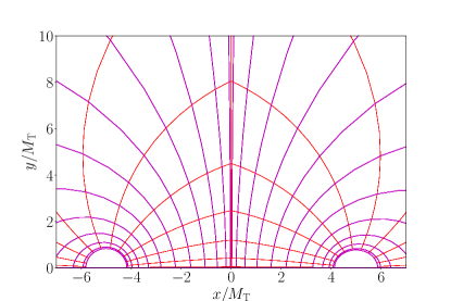
Figure 1: The $\phi=0$ slice in the coordinates we use for the binary black hole configuration qc-sp7cp5 (see Table 1). The black holes are centered at $x=\pm 5M_{\text{T}}$, where $M_{\text{T}}$ is the total mass of the superposed black holes. Lines of constant $A_{\text{Ans}}$ and $B_{\text{Ans}}$ are shown using purple and red, respectively. The excision surfaces are ellipsoids located at $A_{\text{Ans}}=0$. The grid is separated into two computational subdomains that meet along the $yz$-plane (seen here only as the line $x=0$).

As in Lovelace et al. (2008), we impose boundary conditions on the excision surface such that the excision surface coincides with the apparent horizon of each black hole in the solved binary black hole initial data. We thus set the excision surface around each black hole such that it coincides with the event horizon of the boosted Kerr-Newman black hole used in the superposed metric. We do this by numerically solving for a freely specifiable function $\sigma_{A}(B_{\text{Ans}},\varphi)$ that appears in the coordinate transformation between Cartesian coordinates $(x,y,z)$ and Ansorg coordinates $(A_{\text{Ans}},B_{\text{Ans}},\varphi)$. Specifically, we solve for $\sigma_{A}$ such that the horizon equation

$$\dfrac{\|\,\mathbf{r}_{\mathcal{S}}-(\hat{\bm{\chi}}\cdot\mathbf{r}_{\mathcal{S}})\,\hat{\bm{\chi}}\,\|^{2}}{r_{+}^{2}+M^{2}\chi^{2}}+\dfrac{(\hat{\bm{\chi}}\cdot\mathbf{r}_{\mathcal{S}})^{2}}{r_{+}^{2}}=1,$$ (25)

is satisfied on each excision surface. Here, $\mathbf{r}_{\mathcal{S}}$ is the coordinate vector pointing from the black hole center to a point on the excision surface (located at $A_{\text{Ans}}=0$). For a black hole hole with nonzero velocity, we apply the appropriate Lorentz transformation to $\mathbf{r}_{\mathcal{S}}$ to account for the length contraction of the horizon due to the boost. Further, $M$, $\chi$, and $\hat{\bm{\chi}}$ represent the black hole’s mass, the magnitude of its dimensionless spin, and the unit vector along the spin axis, respectively. Additionally, $r_{+}$ is the radius of the outer horizon of a Kerr-Newman black hole given by

$$r_{+}=M+M\sqrt{1-\chi^{2}-\mathcal{Q}^{2}},$$ (26)

where $\mathcal{Q}:=Q/M$, and $Q$ is the charge of the Kerr-Newman black hole.

III.2 Computing diagnostics

In order to characterize our initial datasets and control our initial data parameters, we compute the ADM mass and linear and angular momenta of the initial data. We also compute quasilocal measures of the mass and spin of each individual black hole.

To compute the ADM mass, we follow Marronetti et al. (2007) in obtaining a more numerically accurate expression by writing the original surface integral at infinity as the sum of a volume integral and surface integrals over the excision surfaces and removing the second derivatives of the conformal factor using the Hamiltonian constraint. We correct the expressions from that paper for a flipped pair of indices in the integrand of the surface integral and generalize to the conformally curved case; cf. the original versions of the expressions in Yo et al. (2002). In addition, we also incorporate the source terms arising from the Hamiltonian constraint to obtain

$$\begin{split}M_{\rm ADM}&=\dfrac{1}{16\pi}\int_{\mathcal{V}}\biggl{[}(1-\psi)~{}\tilde{R}+\tilde{\Gamma}^{k}~{}\tilde{\Gamma}^{i}_{~{}ki}-\tilde{\Gamma}^{ikj}\tilde{\Gamma}_{kij}+\psi^{-7}\tilde{A}^{jk}\tilde{A}_{jk}+\psi^{5}\left(16\pi\rho-\dfrac{2}{3}K^{2}\right)\biggr{]}\sqrt{\tilde{\gamma}}~{}dV\\ &\quad+\dfrac{1}{16\pi}\sum_{A=1}^{2}\oint_{\mathcal{S}_{A}}\psi^{4}(\tilde{\Gamma}^{k}-\tilde{\Gamma}^{ik}_{~{}~{}~{}i}-8~{}\tilde{\nabla}^{k}\psi)\sqrt{\tilde{h}}~{}dS_{k},\end{split}$$ (27)

where $\tilde{R}$ and $\tilde{\Gamma}^{i}_{jk}$ are the Ricci scalar and Christoffel symbols computed using the conformal metric and $\tilde{\Gamma}^{i}:=\tilde{\gamma}^{jl}\tilde{\Gamma}^{i}{}_{jl}$. Additionally, $\mathcal{V}$ is the region outside the excision surfaces and $dV$ is the volume element in flat space.

To compute the ADM linear and angular momentum, we follow Ossokine et al. (2015), adding the relevant source terms due to the presence of the EM fields to get

$$P^{i}_{\rm ADM} =\frac{1}{8\pi}\sum_{A=1}^{2}\oint_{\mathcal{S}_{A}}P^{ij}\,dS_{j}-\frac{1}{8\pi}\int_{\mathcal{V}}G^{i}\,dV,$$ (28a)

$$J^{z}_{\rm ADM} =\frac{1}{8\pi}\sum_{A=1}^{2}\oint_{\mathcal{S}_{A}}(xP^{yj}-yP^{xj})\,dS_{j}$$ (28b)

$$\quad-\frac{1}{8\pi}\int_{\mathcal{V}}(xG^{y}-yG^{x})\,dV,$$

where $J^{x}_{\rm ADM}$ and $J^{y}_{\rm ADM}$ are obtained by cyclic permutations of $(x,y,z)$ in the above equation, and

$$P^{ij} :=\psi^{10}(K^{ij}-K\psi^{-4}\tilde{\gamma}^{ij}),$$ (29a)

$$G^{i} :=\tilde{\Gamma}^{i}_{jk}P^{jk}+\tilde{\Gamma}^{j}_{jk}P^{ik}-2\tilde{\gamma}_{jk}P^{jk}\tilde{\gamma}^{il}\partial_{l}(\ln\psi)-8\pi J^{i}.$$ (29b)

As in Ossokine et al. (2015), we apply a rolloff to the volume integrands at large radii in Eqs. (28) to reduce the contributions from numerical noise in the regions near infinity where the integrand is small and the volume element is large. Specifically we set

$$G^{i}_{\text{rolloff}}=\begin{cases}G^{i}&\text{if $r\leq R_{c}$}\\ (R_{c}^{2}/r^{2})~{}G^{i}&\text{if $r>R_{c}$},\end{cases}$$ (30)

where $r$ is the coordinate distance from the origin, and $R_{c}$ is the roll-off radius. We apply the same roll-off to the volume integrand in Eq. (27). We set $R_{c}=500M_{\text{T}}$, where $M_{\text{T}}$ is the sum of the masses of the two superposed Kerr-Newman black holes.

We also compute the quasilocal mass and spin of the black holes in the standard way, through integrals over the excision surfaces, with just a small generalization to the charged case. Specifically, we compute the irreducible mass of the horizon

$$M_{\text{irr}}=\sqrt{\frac{\mathcal{H}}{16\pi}},$$ (31)

where $\mathcal{H}$ is the area of the horizon. We also compute the angular momentum of the horizon $\mathcal{J}^{k}$ using the standard isolated horizon integral Schnetter et al. (2006) with the contribution from the EM fields as in Ashtekar et al. (2001), giving

$$\mathcal{J}^{k}=\frac{1}{8\pi}\oint_{\mathcal{S}_{\text{A}}}[K_{ij}+2(\mathcal{A}_{\rm sp})_{i}E_{j}]\,\xi^{i}_{~{}(k)}\sqrt{h}\,dS^{j},$$ (32)

where $(\mathcal{A}_{\rm sp})_{i}$ is given by Eq. (17) and $\xi^{i}_{~{}(k)}$ are the flat space Killing vectors defined in Eq. (10). The sign of the EM term is opposite the one given in Ashtekar et al. (2001), since we found that this gives the correct result for an isolated Kerr-Newman black hole. We presume that this is due to a difference in sign convention, particularly since Bozzola and Paschalidis (2019, 2021b) use the same sign as Ashtekar et al. (2001), but have not been able to find the exact source of this difference. We then compute the horizon mass, often known as the Christodoulou-Ruffini mass, $M_{\text{Chr}}$ Christodoulou and Ruffini (1971), using

$$M_{\text{Chr}}^{2}=\left(M_{\text{irr}}+\frac{Q^{2}}{4M_{\text{irr}}}\right)^{2}+\frac{\mathcal{J}^{2}}{4M_{\text{irr}}^{2}},$$ (33)

where $\mathcal{J}$ the magnitude of the angular momentum given by Eq. (32), and $Q$ is the horizon charge given by Eq. (21) (computed using the solved electric field). In Sec. IV, we use the sum of the Christodoulou masses, denoted $M_{\rm{T},\rm{C}}$, which gives the total mass of the binary at infinity.

III.3 Controlling BH spin and ADM linear momentum

In Sec. II.1.3, we introduced two parameters in the boundary conditions, $v_{0}^{i}$ in Eq. (8) and $\Omega_{r}^{i}$ in Eq. (II.1.3), which we use to control the ADM linear momentum and the black hole spins, respectively. We discuss how we set them here. As in Ossokine et al. (2015), we iteratively set $v_{0}^{i}$ in Eq. (8) to drive the ADM linear momentum to zero. However, we use a simpler iterative procedure, setting

$$v_{0,n+1}^{i}=v_{0,n}^{i}-\frac{P_{\text{ADM},n}^{i}}{M_{\text{T}}},$$ (34)

where $n$ indexes the Newton iterations. We start the iteration from $v_{0,0}^{i}=0$.

We similarly drive the dimensionless spins to their desired values (those of the superposed Kerr-Newman metrics) by adjusting $\Omega_{r}^{i}$ using a simple iteration inspired by the form of the Kerr-Newman horizon angular velocity Newman and Adamo (2014). We start with the angular velocity of the Kerr-Newman spacetime used in the superposition

$$\Omega_{r,0}^{i}=\frac{\mathcal{J}^{i}_{\text{KN}}}{4M_{\text{Chr, KN}}M_{\text{irr, KN}}^{2}},$$ (35)

where $M_{\text{irr, KN}}$, $M_{\text{Chr, KN}}$, and $\mathcal{J}^{i}_{\text{KN}}$ are the irreducible mass, horizon mass (i.e., Kerr-Newman mass parameter), and angular momentum of each superposed black hole, respectively. We then iteratively update $\Omega_{r}^{i}$ using

$$\Omega_{r,n+1}^{i}=\Omega_{r,n}^{i}+\frac{M_{\text{Chr},n}^{2}\chi^{i}_{\text{KN}}-\mathcal{J}_{n}^{i}}{4M_{\text{Chr},n}M_{\text{irr},n}^{2}},$$ (36)

where, as in Eq. (34), $n$ indexes the Newton iterations. Thus, e.g., $\mathcal{J}_{n}^{i}$ is the horizon angular momentum recomputed after the $n^{\text{th}}$ iteration on the excision surface under consideration. Additionally, $\chi^{i}_{\text{KN}}:=\mathcal{J}_{\text{KN}}^{i}/M_{\text{Chr, KN}}^{2}$ is the dimensionless spin vector of the corresponding Kerr-Newman metric used in the superposition.

IV Results

We now discuss the initial data we constructed to test the code, particularly its convergence with resolution, and the exploratory evolutions we performed. We summarize the cases we consider in Tables 1 and 2.

Name	$q$	$\mathcal{Q}_{1}$	$\mathcal{Q}_{2}$	$\bm{\chi}_{1}$	$\bm{\chi}_{2}$	$M_{\text{T}}\Omega_{0}$	$d/M_{\text{T}}$	$\dot{a}_{0}$	$\zeta$	Evol
qc-sp5	1	0	$0$	(0, 0, 0.50)	(0, 0, 0.50)	0.01941	10	$\hphantom{-}0.006531$	0.5	BAM
qc-hs	1.16	0	$0$	(0, 0, 0.69)	(0, 0, 0.79)	0.02848	16	$0$	1.25	–
qc-hc	1.16	0.97	$-0.97$	(0, 0, 0)	(0, 0, 0)	0.02848	10	$0$	2	–
qc-mc	1.16	0.59	$-0.45$	(0, 0, 0)	(0, 0, 0)	0.02848	10	$0$	2	–
qc-sp7cp5	1.16	0.56	$-0.43$	(0, 0.69, 0)	(0.47, 0, 0)	0.02848	10	$0$	2	–

Table 1: Summary of the parameters of the initial data sets for orbiting binaries (“qc” for “quasicircular”), also indicating the case for which we performed a test evolution with BAM. Here $\mathcal{Q}_{A}$ and $\bm{\chi}_{A}$ are the dimensionless charge and spin on black hole $A$, respectively. Additionally, $q$, $\Omega_{0}$, and $\dot{a}_{0}$ correspond to the mass ratio, angular velocity, and radial velocity of the binary, respectively. Finally, $d$ is the separation between the two black holes and $\zeta$ is the attenuation width parameter defined in Eq. (37). We set the velocity of each black hole using the Newtonian expression in terms of $\Omega_{0}$ and $d$.

Name	$\mathcal{Q}_{1}=\mathcal{Q}_{2}$	$v$	Evol
ho-v0q0	0.0	0.0	HAD, BAM
ho-v0qp1	0.1	0.0	HAD
ho-v0qp3	0.3	0.0	HAD
ho-v0qp5	0.5	0.0	HAD
ho-vp1q0	0.0	0.1	HAD
ho-vp3q0	0.0	0.3	HAD

Table 2: Summary of the parameters of the initial data sets for head-on collisions (abbreviation “ho” ) of equal-mass, equal-charge, nonspinning binaries we constructed and performed test evolutions of with HAD and BAM. Here, $v$ is the magnitude of the velocity of each black hole. We set $d=10M_{\text{T}}$ and $\zeta=2$ for all configurations listed here and set $\dot{a}_{0}=-v/d$ for the head-on collisions.

IV.1 Initial Data

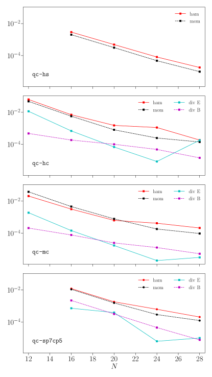
Figure 2: Convergence of the constraint residuals for four different binary configurations, a highly spinning case (qc-hs), highly charged (qc-hc) and moderately charged (qc-mc) cases, and a more generic charged and spinning case (qc-sp7cp5). In all cases, we show the Hamiltonian and momentum constraints (“ham” and “mom”), and for the charged cases, we also show the electric and magnetic constraints (“div E” and “div B”). The horizontal axis gives the number of points used for each coordinate ($N$) and the vertical axis shows the $L^{2}$ norm of the physical constraints over the entire computational grid (scaled by the total volume of the computational grid). Hence, we scale the $L^{2}$ norm by the square of the total Christodoulou mass $M_{\rm{T},\rm{C}}$. For the momentum constraint, this includes the Euclidean vector norm on the components of the constraint. For $N=12$, the initial data solver does not converge for qc-hs and qc-sp7cp5, since the larger gradients near the horizon from significant spin require more resolution to reach the convergent regime.

To test the convergence of our initial data solver, we consider four representative orbiting configurations: two nonspinning cases with high (qc-hc) and moderate (qc-mc) charge, one uncharged case with reasonably high spins (qc-hs), and finally, a more generic precessing binary with moderate charges and spins (qc-sp7cp5). We choose opposite signs for the charges in the charged cases to increase the asymmetry and thus provide a more stringent test of the solver. We use the same number of points ($N$) in the $A_{\text{Ans}},B_{\text{Ans}}$, and $\phi$ directions for each configuration, and set

$$w_{A}=\zeta\dfrac{M_{A}}{M_{1}+M_{2}}d,$$ (37)

for the attenuation weights in Eqs. (6), (16), and (17). Here, $\zeta$ is a dimensionless free parameter and $d$ is the coordinate distance between centers of the two black holes. We set $\Omega_{0}$ and $\dot{a}$ in Eq. (II.1.3) by performing iterative eccentricity reduction. For the other initial data sets, we set $\Omega_{0}$ using the PN expression in Mroué and Pfeiffer (2012) for qc-sp5, and set $\dot{a}=0$. As we discuss later, we do not expect these settings to give low-eccentricity initial data, so we do not attempt to include the effects of the charge. In Fig. 2 we show the convergence of the geometric (Hamiltonian and momentum) and EM constraint residuals for all the four cases. We find the expected exponential (spectral) convergence at low resolutions, but find slower convergence at higher resolution.

In particular, for the geometric constraints, we see spectral convergence only up to $N=20$ for the highly charged case (qc-hc). For the highly spinning case (qc-hs), the convergence is exponential up to $N=28$. For the binary with more generic parameters (qc-sp7cp5), the rate of convergence is better than for the highly charged case (possibly due to the fact that the more generic system is less extreme), but the Hamiltonian constraint shows subexponential decay after $N=20$. While this looks similar to the subexponential convergence found for the construction without attenuation functions in Lovelace (2009), the cause of the slower than expected convergence in our case must be due to a different cause: We use attenuation functions when superposing both the metric and the electromagnetic fields, which ensures that they fall off rapidly at infinity, so there is no possibility for the logarithmic term in the solution that caused the subexponential convergence in Lovelace (2009). In fact, we do not even have the co-rotation term in the outer boundary condition for the shift that leads to that logarithmic term in the Hamiltonian constraint when combined with the $1/r$ falloff of the conformal metric without attenuation functions. One other possible cause that we can exclude is the adjustments to $v_{0}$ and $\Omega^{i}_{r}$ that we perform during the Newton iterations. We disabled these iterations but found no improvement in the speed of convergence. For the EM constraints, we see spectral convergence for electromagnetic constraints up to $N=24$ for all the configurations except for qc-sp7cp5 at $N=20$. The rate of exponential decay, however, is much slower for the magnetic constraint than for the electric constraint.

Figure 3: The electric (top panel) and magnetic (bottom panel) fields (multiplied by $M_{\rm{T},\rm{C}}$) at the grid points around the two black holes in the $xy$-plane for qc-sp7cp5. The arrows represent the unit vectors of the projection of the field into the $xy$-plane. The magnitude of the projection is shown by the color scheme. The black hole on the left (right) has its spin aligned along the $x$- ($y$-) axis giving rise to two magnetic dipole moments aligned with the two spin axes.

We also illustrate the solved electric and magnetic fields for the qc-sp7cp5 case, with its oppositely charged, spinning black holes, in Fig. 3. As one would expect, we observe an overall electric dipole moment aligned along the axis joining the two black holes, and a magnetic dipole for each black hole aligned with its spin axis. Further, the magnetic field due to the orbital motion of the black holes (not visible in the figure, since it is perpendicular to the plane plotted and thus projected out) is consistent with the magnetic field around two charges with different signs moving in opposite directions. Unsurprisingly, we find the largest corrections to the unsolved superposed electric and magnetic fields near each black hole.

Finally, we check how well the isolated horizon condition on the EM fields at the horizon [Eq. (23)] is satisfied in our initial data. We do this by computing the $L^{2}$ norm of the residual over the horizon, as well as the version with the sign reversed, for comparison. Specifically, we define

$$Z^{\pm}_{i} :=E_{i}^{\parallel}\pm(s\times B)_{i},$$ (38a)

$$\text{EB}_{\text{res},\pm}^{2} :=\oint_{\mathcal{S}_{\text{A}}}\gamma^{ij}Z^{\pm}_{i}Z^{\pm}_{j}\,\sqrt{h}\,s^{k}dS_{k},$$ (38b)

where $\text{EB}_{\text{res},+}/\text{EB}_{\text{res},-}$ gives a dimensionless measure of how well the relation is satisfied on each excision surface. We found the ratio to be the lowest (0.04) for the larger black hole in qc-sp7cp5 and the largest (0.09) for the smaller black hole in qc-mc. Additionally, in the nonspinning cases, we found this ratio to depend on the asymmetry of the magnitude of the two dimensionless charges. Hence, even though the black holes in qc-mc have smaller charges than in qc-hc, we find the deviations from the isolated horizon condition to be larger for qc-mc which has the largest dimensionless charge ratio among the charged, nonspinning configurations.

IV.2 Exploratory Evolutions

We performed test evolutions of vacuum data initial data using the BAM code Brügmann et al. (2008). For the charged case, we used the HAD code Liebling et al. (2020) to evolve head-on collisions of charged black holes. Both of these codes, however, are designed to evolve puncture initial data, and hence require black hole filling to evolve our excision initial data (see, e.g., Brown et al. (2009)). We used BHfiller (described in Sec. 3.2 of Reifenberger (2013)) to fill inside the excision surfaces in BAM. We had to generalize the filling algorithm slightly to account for our nonspherical excision surfaces (see Appendix B). HAD uses a different approach to filling, described in Appendix C.

IV.2.1 Uncharged binary black holes in orbit

For the uncharged case, we evolved an equal-mass, equal-aligned-spin quasicircular binary inspiral in orbit (qc-sp5, with dimensionless spins of $0.5$ in the direction of the orbital angular momentum) using BAM with the BSSN formulation of the equations and the standard puncture gauge. For this initial test, we used $16$ points in each direction to construct the initial data using SGRID. For the evolution, we use seven refinement levels with three moving levels and four fixed levels. Each refinement level has half the grid spacing of the previous one with a minimum grid spacing of $0.0625M_{\text{T}}$. The outer boundary of the computational domain is at $\sim 250M_{\text{T}}$. We use fourth-order spatial finite differencing and fourth-order integration in time, with a Courant factor of $0.25$. We extract the gravitational waves at a radius of $r_{\text{ext}}=50M_{\text{T}}$.

We reduced the eccentricity by adjusting $\Omega_{0}$ and $\dot{a}$ using the iterative method in Pfeiffer et al. (2007), where we measure the eccentricity using the puncture tracks. We found that the eccentricity one obtains from the post-Newtonian values for $\Omega_{0}$ and $\dot{a}_{0}$ given in Mroué and Pfeiffer (2012) is large enough that the iterative method does not reduce the eccentricity when starting from those values. We thus adjusted those parameters by hand until the eccentricity was small enough that the iterative method produced further reductions of the eccentricity. We obtained an eccentricity of about $0.06$, which is relatively large, compared to the eccentricities needed for waveform modeling (e.g., the eccentricities of $\sim 10^{-3}$ achieved for some of the simulations produced in Husa et al. (2016)). While we could have carried out further iterations of the eccentricity reduction procedure, we chose not to for this initial test. In particular, the unusual nature of the eccentricity reduced setup we obtained, where the coordinate separation between the punctures increases before decreasing when the data are evolved, deserves more careful investigation.

In Figs. 4 and 5, we show the real part of the quadrupolar ($l=m=2$) mode of the Weyl scalar $\psi_{4}$, and the puncture tracks for the last $\sim 8$ orbits before merger, respectively, for qc-sp5, to illustrate that they are qualitatively as expected. As is clear from the nearly overlapping puncture tracks, the binary still has a relatively large eccentricity (consistent with the value of $\sim 0.06$ obtained above). An important consideration when constructing initial data is how much the properties of the binary (e.g., black hole spin) change during early states of the evolution, as the system relaxes and emits junk radiation. We observed that the dimensionless spins settle to $0.49$ (compared to the desired value of $0.5$) after the first $900M_{\rm{T,C}}$ during which the system relaxes by emitting junk radiation. The relative error between the computed and desired spins decreases through the first $900M_{\rm{T,C}}$ and is $\sim 6\%$ at its maximum.

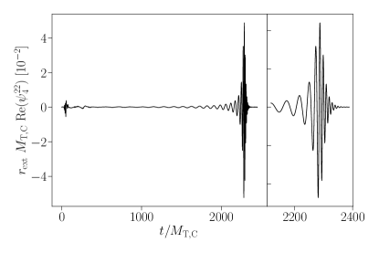
Figure 4: The real part of the $l=m=2$ mode of the Weyl scalar $\psi_{4}$ from the uncharged, quasicircular, aligned-spin evolution qc-sp5. The left panel shows the complete waveform, and the right panel shows the waveform around the merger.

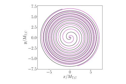
Figure 5: Puncture tracks of the two black holes for the qc-sp5 evolution. The tracks show approximately 8 orbits before merger and demonstrate the nonnegligible eccentricity of $\sim 0.06$.

IV.2.2 Head-on collisions of charged binary black holes

We now consider head-on collisions of charged black holes. Unfortunately, we were unable to produce evolutions of orbiting binaries with HAD, even when evolving a vacuum case for which the BAM evolution orbited. The evolutions of orbiting initial data with HAD initially resemble quasi-circular orbits, but quickly the trajectory of the black holes becomes nearly head-on. This failure to orbit may be due to the method of filling the excised interior developed in HAD for this project, described in Appendix C. In particular, even though Brown et al. (2009) showed that the constraint violations from the filling do not propagate outside the horizon in BSSN, the finite difference stencils extend inside the horizon and thus the filling affects the evolution through the derivatives of the fields. In fact, Brown et al. (2009) finds that one needs the filling to extend out to a coordinate radius at most $0.4$ times the horizon radius in order for the filling not to affect the evolution (though the isotropic coordinate system of their initial data is rather different from our Kerr-Schild one). However, for our initial data construction, the apparent horizon coincides with the excision surface, and so it is necessary to fill all the way to the apparent horizon. It thus might be worthwhile to extend the construction to allow for the excision surface to be inside the apparent horizon by using negative expansion boundary conditions, as in Varma et al. (2018).

For our tests of charged, head-on collisions, we evolved equal-mass, equal-charge, nonspinning binaries, as well as some uncharged, boosted head-on collisions (see Table 2 for an overview of these cases). The charged cases allow us to compare with previous numerical work Zilhao et al. (2012); Zilhão et al. (2014). In particular as discussed below, analytical scalings found in their work agree well with our results.

We used a resolution of $(18,18,12)$ points in the $A_{\text{Ans}},B_{\text{Ans}}$, and $\phi$ directions to generate the initial data in SGRID. The HAD evolutions used four refinement levels and each refinement level has half the grid spacing of the previous one, with a minimum grid spacing of $0.0891M_{\text{T}}$. The outer boundary of the computational domain is at $\sim 72M_{\text{T}}$. We used fourth-order spatial finite differencing and third-order integration in time with a Courant factor of $0.25$. We extract gravitational and electromagnetic waves at $r_{\text{ext}}=50M_{\rm{T}}$. For the electromagnetic emission, we compute the scalar function $\Phi_{2}$ that contains the transverse radiative degrees of freedom of the electric field, in the asymptotic limit Newman and Penrose (1962). The details of the evolution system (BSSN with the standard puncture gauge plus constraint damping for the EM equations) and code are described in Hirschmann et al. (2018) which evolved binary black holes in Einstein-Maxwell-dilaton theory. For these evolutions we simply set the dilaton coupling parameter $\alpha$ to zero.

In Fig. 6, we compare the quadrupolar mode of $\psi_{4}$ between HAD and BAM evolutions for a head-on collision of two uncharged black holes starting from rest. Both waveforms are extracted at $r_{\text{ext}}=50M_{\text{T}}$. Note that while the junk radiation profiles show some differences, the merger section of the waveform is in good agreement. While we have not attempted to quantify the error budgets of the two simulations, we anticipate that the differences seen are well within the combined error budget, particularly since these are not particularly high resolution simulations and have rather small GW extraction radii.

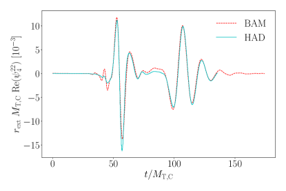
Figure 6: A comparison of the real part of the $l=m=2$ mode of $\psi_{4}$ from the head-on collision of two uncharged black holes starting from rest (ho-v0q0) evolved using HAD and BAM. The waveforms are not aligned in any way.

In Fig. 7, we show the $l=2,m=0$ mode of gravitational and electromagnetic radiation from the head-on collisions of binary black holes for various charge-to-mass ratios, including the $\mathcal{B}:=1-\mathcal{Q}^{2}$ Newtonian scaling that Zilhao et al. (2012) found to account for most of the amplitude’s dependence on the charge. In Zilhao et al. (2012) the authors place the black holes on the $z$-axis, whereas in our setup, we place them on the $x$-axis. Thus, to make a direct comparison with Zilhao et al. (2012), we transformed our waveforms to place the black holes along the $z$-axis using the quaternionic package Boyle (2017, 2016). We find that the waveforms from our evolutions satisfy the scalings found in Zilhao et al. (2012) for the merger-ringdown portion of the waveform with reasonable accuracy, though with larger differences than in Zilhao et al. (2012). Specifically, Zilhao et al. (2012) found differences of at most $2\%$ compared to the scaling for charges up to $98\%$ of maximal. In our simulations, however, we found the differences to be larger (up to $\sim 3\%$) for charges up to $50\%$ of maximal, though our evolutions are preliminary, and we did not attempt to assess convergence, in addition to the issues with the effects of the filling mentioned previously.

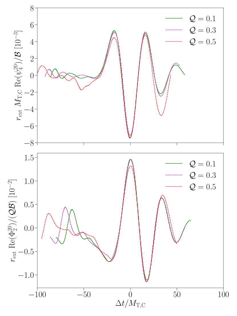
Figure 7: The $l=2,m=0$ mode (in the rotated frame with the black holes on the $z$-axis) of $\psi_{4}$ (top panel) and $\Phi_{2}$ (bottom panel) aligned at merger using the peak of the amplitude of the real part of the waveform. These waveforms correspond to head-on collisions of equal-mass, nonspinning charged black holes evolved using HAD for different charge to mass ratios, i.e., ho-v0qp1, ho-v0qp3, and ho-v0qp5.

IV.2.3 Head-on collisions of boosted uncharged binary black holes

We also considered head-on collisions of uncharged black holes boosted towards each other with velocity parameters of $0.1$ and $0.3$, as well as an unboosted case, for comparison. In the boosted cases, the assumption that the system is in quasi-equilibrium breaks down, and hence our choice of setting $u_{ij}=0$ becomes increasingly inaccurate for larger initial velocities. However, we still find that increasing the initial velocity decreases the time to merger, so we present these results as a further example of the code’s ability to generate initial data for generic binaries.

To quantify the effects of the boost, we consider the time to merger for each of the simulations ($t_{\rm{sim}}$), which we compare with the Newtonian estimate ($t_{\rm{m}}$), as in the charged case considered above. To compute the merger time from the simulations, we use the time it takes for each black hole to reach the origin, using the minimum of the lapse as a proxy for the location of the black hole. To compute the Newtonian estimate for the merger time, we use energy conservation. Specifically, we generalized the calculation done in Zilhao et al. (2012) to include boosts. For two black holes each with mass $M/2$ and charge $Q/2$ placed initially at $x=\pm d/2$ with initial velocities of $v_{0}$, conservation of energy implies

$$M\dot{x}^{2}-\dfrac{M^{2}\mathcal{B}}{4x}=Mv_{0}^{2}-\dfrac{M^{2}\mathcal{B}}{2d},$$ (39)

where $x$ is the position of one of the black holes and the overdot denotes a time derivative. Rearranging and integrating both sides, we get

$$t_{\text{m}}=\dfrac{\mathcal{B}M}{\mathcal{Z}^{3}}\left[\dfrac{\pi}{2}-\arctan\left(\dfrac{2v_{0}}{\mathcal{Z}}\right)\right]-\dfrac{2v_{0}d}{\mathcal{Z}^{2}},$$ (40)

where

$$\mathcal{Z}:=\sqrt{\dfrac{\mathcal{B}M}{d}-4v_{0}^{2}},$$ (41)

where we evaluate the arctangent on the right-hand side of the branch cut (so its real part is $\pi/2$) for the cases where $\mathcal{Z}$ is imaginary, which ensures the result is always real. For the unboosted case (ho-v0q0), we find the time from the simulation, $t_{\rm{sim}}$, to be larger than $t_{\rm{m}}$ with a relative error $\sim 18\%$. For the boosted cases, similar to the charged case, we scale both $t_{\rm{sim}}$ and $t_{\rm{m}}$ by the corresponding computation for the unboosted case and denote these scaled values by $\tilde{t}_{\rm{m}}$ and $\tilde{t}_{\rm{sim}}$, respectively. We find $\tilde{t}_{\rm{sim}}$ to be larger than $\tilde{t}_{\rm{m}}$ for both ho-vp1q0 and h0-vp3q0, and the relative error between them to be $\sim 57\%$ for ho-vp1q0, and $\sim 103\%$ for h0-vp3q0.

There could be several reasons behind these large discrepancies for both charged and uncharged, boosted cases. In particular, our method to infer the collision time from the numerical evolutions likely overestimates the merger time compared, e.g., to using the first appearance of a common apparent horizon to determine the merger time, as was done in Zilhao et al. (2012). Additionally, for the boosted cases, as mentioned before, we use the quasi-equilibrium approximation ($u_{ij}=0$) beyond its regime of validity. This, in addition to the issues with filling the black holes described earlier and the effects of junk radiation, can result in the black holes in the simulation having different initial velocities than those used in the construction of the initial data.

As a rough check, we estimated the initial velocities of the black holes using the location of the black hole and finite differencing. We started at $13.5M_{\rm{T},\rm{C}}$ to be after the initial transients and considered a time span of $7M_{\rm{T},\rm{C}}$, chosen by eye so that a constant velocity given by the finite difference gives a good approximation to the time dependence of the black holes’ positions. We found the initial velocities to be $0.087$ and $0.130$ for ho-vp1q0 and h0-vp3q0, respectively. For h0-v0q0, we found the computed velocity to be zero, in agreement with the velocity used in the computation of the initial data. Using these velocities in the merger time calculation reduced the computed merger time as well as the relative error between $\tilde{t}_{\rm{m}}$ and $\tilde{t}_{\rm{sim}}$ to $\sim 23\%$ and $\sim 74\%$ for h0-vp1q0 and h0-vp3q0, respectively.

V Summary and Future Work

In this paper, we constructed initial data for spinning, charged, orbiting binary black holes by extending the superposed Kerr-Schild construction for vacuum binary black hole initial data presented in Lovelace (2009). In contrast to previous work Bozzola and Paschalidis (2019) which constructed conformally flat puncture initial data, our construction gives conformally curved initial data with excision. Our approach—in addition to providing a completely independent method to construct charged binary black hole initial data—offers several advantages over the approach used in Bozzola and Paschalidis (2019), e.g., better control over the physics through the boundary conditions at the excision surface and the ability to construct binary initial data with larger spin, above the Bowen-York limit. It also provides a complementary implementation of the original vacuum construction in Lovelace (2009) with a different numerical setup and a slightly different choice of boundary conditions. Specifically, we transfer the corotation and expansion terms from the outer to the inner boundary condition for the shift.

We tested our initial data construction for several cases including binaries with highly charged black holes and black holes with both charge and spin. We performed convergence tests and found our initial data implementation gives exponential convergence for low resolutions, but slower convergence for higher resolutions. We also carried out exploratory evolutions of charged and uncharged initial data using two different evolution codes (BAM in the uncharged case and HAD with both charged and uncharged data). Here we evolved a quasicircular uncharged binary without charge with BAM, but were unable to obtain an orbiting evolution with HAD even in the uncharged case, which we attribute to the differences in filling inside the excision surfaces in the two codes. Thus, in the charged case, we considered head-on collisions with different charge-to-mass ratios and found that our numerical results are consistent with the simple (Newtonian) analytic scalings presented in Zilhao et al. (2012). Our estimates of the time of collapse for boosted, head-on collisions differed significantly from a similar Newtonian estimate. However, a number of factors particular to these results might explain such differences, and the collapse time decreased with increasing initial velocity as would be expected.

There are several improvements one could make to our initial data construction. For example, it would be useful to understand and mitigate the loss of exponential convergence at higher resolutions, especially for binaries with large charge. This might require conformally rescaling the EM quantities as was done in Alcubierre et al. (2009); Bozzola and Paschalidis (2019), and careful handling of the regularity conditions at the computational domain boundaries, where the gradients of electric constraint violations are the largest. In order to generate waveforms for gravitational wave data analysis, we might need a better initial guess for the eccentricity reduction procedure that does not lead to the unusual eccentricity reduced solution we obtained here. We will also need to resolve the outstanding issues with black hole filling in HAD. In particular, it would be worth exploring if setting the excision surface to be inside the apparent horizon, as in Varma et al. (2018), mitigates the issues we encountered while evolving our excision initial data using puncture methods.

As discussed in Sec. I, one goal is to use our initial data to compute low-eccentricity charged binary black hole waveforms that are sufficiently accurate for data analysis applications. Such waveforms will allow us to check how sensitive current LIGO-Virgo tests Abbott et al. (2021c, d) are to completely consistent, parameterized deviations from GR. To evolve our charged initial data, another possibility—in addition to HAD—would be the LEAN code Sperhake (2007); Zilhão et al. (2014); Zilhao et al. (2012) which would allow us to compute the quasilocal mass, charge, and spin of black holes during evolution.

Our construction can also be extended to construct initial data for binary black holes in Einstein-Maxwell-dilaton theory. In general, this would require superposing numerically constructed single black hole solutions for spinning black holes Kleihaus et al. (2003, 2004), but analytical solutions are known for black holes without spin and for spinning black holes with specific values of the coupling parameter Frolov et al. (1987), so an initial implementation could focus on these simpler cases. There are no additional constraint equations to solve for the dilaton field, just additional source terms in the Hamiltonian and momentum constraints. However, one might ultimately want to generalize the construction to also allow the dilaton field to be adjusted as part of the solve, to obtain a better approximation to quasiequilibrium. Evolutions with such initial data would improve upon the existing work by Hirschmann et al. Hirschmann et al. (2018) using approximate initial data, and also allow for comparisons with analytical work Khalil et al. (2018); Julié (2018).

Appendix A Kerr-Newman black hole in Kerr-Schild form

In Sec. II, we discuss the superposition of Kerr-Newman metrics for the choice of freely specifiable variables. Here, we give the relevant expressions for completeness. In the $3+1$ setting, the spatial metric and extrinsic curvature for a stationary Kerr-Newman black hole in Kerr-Schild coordinates are given by Debney et al. (1969); Newman and Adamo (2014)

$$\gamma_{ij} = f_{ij}+2Hl_{i}l_{j},$$ (42a)

$$K_{ij} = \dfrac{1}{2\alpha}\left(\nabla_{i}\beta_{j}+\nabla_{j}\beta_{i}-\partial_{t}\gamma_{ij}\right),$$ (42b)

where the lapse $\alpha$ and the shift $\beta_{i}$ are given by

$$\alpha=\dfrac{1}{\sqrt{1+2Hl_{0}^{2}}},\qquad\beta_{i}=2Hl_{0}l_{i},$$ (43)

writing these in a form that makes it easy to compute their boosted form, following Bonning et al. (2003). In the above equations, the metric function $H$ and the null vector $l_{\mu}\doteq\{l_{0},l_{i}\}$ are given by

$$H={} \dfrac{Mr^{3}-(Qr)^{2}/2}{r^{4}+\left(\mathbf{a}\cdot\mathbf{x}\right)^{2}},$$ (44a)

$$l_{\mu}\doteq{} \Big{\{}1,\dfrac{r\left[\mathbf{x}-\left(\mathbf{\hat{a}}\cdot\mathbf{x}\right)\mathbf{\hat{a}}\right]-\left(\mathbf{a}\times\mathbf{x}\right)}{r^{2}+a^{2}}+\dfrac{\left(\mathbf{\hat{a}}\cdot\mathbf{x}\right)\mathbf{\hat{a}}}{r}\Big{\}},$$ (44b)

where $\mathbf{x}\doteq\{x,y,z\}$ is the three dimensional coordinate vector, $\mathbf{a}=a\,\hat{\mathbf{a}}$ is the angular momentum per unit mass, and $M$ and $Q$ are the mass and charge of the black hole, respectively. Here we use $\doteq$ to denote that we are giving the components of a vector. The parameter $r$ is given by

$$r^{2} =\dfrac{1}{2}(\rho^{2}-a^{2})+\sqrt{\dfrac{1}{4}\left(\rho^{2}-a^{2}\right)^{2}+\left(\mathbf{a}\cdot\mathbf{x}\right)^{2}},$$ (45a)

$$\rho^{2} =x^{2}+y^{2}+z^{2}.$$ (45b)

Note that in Eq. (44b) and in Eq. (A) below, we use the Euclidean cross product. To compute the electric and magnetic fields for a Kerr-Newman black hole, we use the four-potential Newman and Adamo (2014)

$$A_{\mu}\doteq-\dfrac{Qr^{3}}{r^{4}+\left(\mathbf{a}\cdot\mathbf{x}\right)^{2}}{} \Big{\{}1,\dfrac{r\left[\mathbf{x}-\left(\hat{\mathbf{a}}\cdot\mathbf{x}\right)\hat{\mathbf{a}}\right]-\mathbf{a}\times\mathbf{x}}{r^{2}+a^{2}}$$

$$+\dfrac{\left(\hat{\mathbf{a}}\cdot\mathbf{x}\right)\hat{\mathbf{a}}}{r}\Big{\}},$$ (46)

and compute the electric and magnetic field using Alcubierre et al. (2009)

$$E^{\mu}:=-n_{\nu}F^{\nu\mu},\quad B^{\mu}:=-n_{\nu}{}^{*}F^{\nu\mu},$$ (47)

where $n_{\mu}\doteq\left\{\alpha,0,0,0\right\}$ is the four velocity of an Eulerian observer, and $F_{\mu\nu}$ and ${}^{*}F^{\mu\nu}$ are the Faraday tensor and its dual

$$F_{\mu\nu}=\partial_{\mu}A_{\nu}-\partial_{\nu}A_{\mu},\quad{}^{*}F^{\mu\nu}:=-\dfrac{1}{2}\epsilon^{\mu\nu\eta\gamma}F_{\eta\gamma}.$$ (48)

Here $\epsilon^{\mu\nu\eta\gamma}$ is the curved-space Levi-Civita symbol, such that $\epsilon^{0123}=-1/\sqrt{-g}$, where $g$ is the determinant of the full 4-dimensional spacetime metric.

For a boosted Kerr-Newman black hole, we first compute $H$ and the vector quantities $U_{\mu}\in\{l_{\mu},n_{\mu},A_{\mu}\}$ in the boosted coordinates $\bar{x}_{\alpha}$, given by

$$x^{\beta}=\Lambda^{\beta}_{~{}~{}\alpha}\,\bar{x}^{\alpha},$$ (49)

where $x^{\alpha}$ are the inertial (grid) coordinates and $\Lambda^{\beta}_{~{}~{}\alpha}$ is the Lorentz transformation matrix relating the two frames, and then apply the Lorentz transformation to the vectors themselves, i.e.,

$$H(x^{\alpha})={} \bar{H}\bigl{(}[\Lambda^{-1}]^{\beta}_{~{}~{}\alpha}\,x^{\alpha}\bigr{)},$$ (50a)

$$U_{\delta}(x^{\alpha})={} \Lambda^{\gamma}_{~{}~{}\delta}\,\bar{U}_{\gamma}\bigl{(}[\Lambda^{-1}]^{\beta}_{~{}~{}\alpha}\,x^{\alpha}\bigr{)},$$ (50b)

where barred quantities correspond to the boosted frame. We then use Eqs. (42), (43), (47), and (48) to compute the relevant quantities for the boosted black hole.

Appendix B Filling inside excision surfaces in BAM

To fill inside the excision surfaces in BAM, we modified the original BHFiller algorithm (see Chapter 3.2 in Reifenberger (2013) for details) that fills inside spherical excision surfaces to allow for our excision surfaces that are deformed by the black holes’ spin and boosts. Specifically, we first transform from the grid coordinates to coordinates in which the excision surfaces are spherical, then perform the interpolation using BHFiller, and finally transform back to grid coordinates.

The coordinate transformation to coordinates in which the excision surfaces are spherical is a simple linear one and is performed in two steps, first removing the Lorentz contraction due to the boost and then removing the deformation due to the spin. These transformations are both of the form

$$\mathbf{x}\to w_{\perp}\mathbf{x}+(w_{\parallel}-w_{\perp})(\mathbf{x}\cdot\hat{\mathbf{k}})\,\hat{\mathbf{k}},$$ (51)

where the parameters $w_{\parallel}$ and $w_{\perp}$ set the amount of deformation parallel and perpendicular to the symmetry axis given by the unit vector $\hat{\mathbf{k}}$. Specifically, for the Lorentz boost, with velocity $\mathbf{v}$ (and magnitude $v$), one takes $w_{\parallel}=1/\sqrt{1-v^{2}}$, $w_{\perp}=1$, and $\hat{\mathbf{k}}=\hat{\mathbf{v}}$. For the spin deformation, with angular momentum per unit mass of the black hole $\mathbf{a}$ (and magnitude $a$), one takes $w_{\parallel}=1$, $w_{\perp}=r_{+}/\sqrt{r_{+}^{2}+a^{2}}$, and $\hat{\mathbf{k}}=\hat{\mathbf{a}}$, where $r_{+}$ is the coordinate radius of the Kerr outer horizon, given (for Kerr-Newman) in Eq. (26). (Here we only consider Kerr because BAM only evolves the vacuum case.) The inverse transformations are given by using the reciprocals of $w_{\parallel}$ and $w_{\perp}$.

Appendix C Filling inside excision surfaces in HAD

To fill the black hole interiors in HAD, we use an approach seeking to approximate the BHFiller method described in Reifenberger (2013). Using the mask provided by SGRID, we fill only those points flagged as “excised” to avoid throwing away any information from the initial data solver. In particular, the filling algorithm uses four passes through the domain. The first three passes each correspond to one of the coordinate directions ($x$, $y$, and $z$) during which each interior point is updated with a sweep from each side of the hole. For a black hole centered at $(x_{c},y_{c},z_{c})$, the sweep starts at small $x$ and fixed $y$ and $z$. When an excised point is first encountered, the value of the field $u$ at the last un-excised point, $u(x_{0},y,z)$ together with a backward difference estimate of the derivative $\Delta u/\Delta x$ are used to extrapolate points as the sweep proceeds towards $x_{c}$. Similar sweeps in the $y$ and $z$ directions follow as

$${}^{1}u(x,y,z)={} u(x_{0},y,z)+\left(x-x_{0}\right)\frac{\Delta u}{\Delta x}\left(\frac{x-x_{c}}{r_{A}}\right)^{2},$$ (52a)

$${}^{2}u(x,y,z)={} {}^{1}u(x,y_{0},z)+\left(y-y_{0}\right)\frac{\Delta u}{\Delta y}\left(\frac{y-y_{c}}{r_{A}}\right)^{2},$$ (52b)

$${}^{3}u(x,y,z)={} {}^{2}u(x,y,z_{0})+\left(z-z_{0}\right)\frac{\Delta u}{\Delta z}\left(\frac{z-z_{c}}{r_{A}}\right)^{2}.$$ (52c)

This expression is for excision surface $A$; recall that $r_{A}$ is the coordinate distance from the center of that excision surface. These passes serve to approximate the linear extrapolation from the exterior to the center of the black hole along the radial direction. The final pass

$${}^{4}u(x,y,z)=\Gamma\;{}^{3}u(x,y,z)+\left(1-\Gamma\right)u(x_{c},y_{c},z_{c}),$$ (53)

interpolates the extrapolated value with a prescribed central value for the field. This last step is described in Reifenberger (2013) which gives both the form of the interpolating function $\Gamma$ as a function of distance from the center of the black hole and the central values for each of the fields filled. For the electric and magnetic field components, we set the central value to zero.

References

- Abbott et al. (2019a) B. P. Abbott et al. (LIGO Scientific Collaboration and Virgo Collaboration), Phys. Rev. X 9, 031040 (2019a), arXiv:1811.12907 [astro-ph.HE] .
- Abbott et al. (2021a) R. Abbott et al. (LIGO Scientific Collaboration and Virgo Collaboration), Phys. Rev. X 11, 021053 (2021a), arXiv:2010.14527 [gr-qc] .
- Abbott et al. (2021b) R. Abbott et al. (LIGO Scientific Collaboration, Virgo Collaboration, and KAGRA Collaboration), (2021b), arXiv:2111.03606 [gr-qc] .
- Abbott et al. (2019b) B. P. Abbott et al. (LIGO Scientific Collaboration and Virgo Collaboration), Phys. Rev. Lett. 123, 011102 (2019b), arXiv:1811.00364 [gr-qc] .
- Abbott et al. (2021c) R. Abbott et al. (LIGO Scientific Collaboration and Virgo Collaboration), Phys. Rev. D 103, 122002 (2021c), arXiv:2010.14529 [gr-qc] .
- Abbott et al. (2021d) R. Abbott et al. (LIGO Scientific Collaboration, Virgo Collaboration, and KAGRA Collaboration), (2021d), arXiv:2112.06861 [gr-qc] .
- Chua and Vallisneri (2020) A. J. K. Chua and M. Vallisneri, (2020), arXiv:2006.08918 [gr-qc] .
- Perkins et al. (2021) S. E. Perkins, R. Nair, H. O. Silva, and N. Yunes, Phys. Rev. D 104, 024060 (2021), arXiv:2104.11189 [gr-qc] .
- Wang et al. (2021) H.-T. Wang, S.-P. Tang, P.-C. Li, M.-Z. Han, and Y.-Z. Fan, Phys. Rev. D 104, 024015 (2021), arXiv:2104.07590 [gr-qc] .
- Kovács and Reall (2020a) A. D. Kovács and H. S. Reall, Phys. Rev. Lett. 124, 221101 (2020a), arXiv:2003.04327 [gr-qc] .
- Kovács and Reall (2020b) A. D. Kovács and H. S. Reall, Phys. Rev. D 101, 124003 (2020b), arXiv:2003.08398 [gr-qc] .
- East and Ripley (2021a) W. E. East and J. L. Ripley, Phys. Rev. D 103, 044040 (2021a), arXiv:2011.03547 [gr-qc] .
- East and Ripley (2021b) W. E. East and J. L. Ripley, Phys. Rev. Lett. 127, 101102 (2021b), arXiv:2105.08571 [gr-qc] .
- Figueras and França (2021) P. Figueras and T. França, (2021), arXiv:2112.15529 [gr-qc] .
- Okounkova et al. (2020) M. Okounkova, L. C. Stein, J. Moxon, M. A. Scheel, and S. A. Teukolsky, Phys. Rev. D 101, 104016 (2020), arXiv:1911.02588 [gr-qc] .
- Okounkova et al. (2019) M. Okounkova, L. C. Stein, M. A. Scheel, and S. A. Teukolsky, Phys. Rev. D 100, 104026 (2019), arXiv:1906.08789 [gr-qc] .
- Okounkova (2020) M. Okounkova, Phys. Rev. D 102, 084046 (2020), arXiv:2001.03571 [gr-qc] .
- Witek et al. (2019) H. Witek, L. Gualtieri, P. Pani, and T. P. Sotiriou, Phys. Rev. D 99, 064035 (2019), arXiv:1810.05177 [gr-qc] .
- Silva et al. (2021) H. O. Silva, H. Witek, M. Elley, and N. Yunes, Phys. Rev. Lett. 127, 031101 (2021), arXiv:2012.10436 [gr-qc] .
- Gálvez Ghersi and Stein (2021) J. T. Gálvez Ghersi and L. C. Stein, Phys. Rev. E 104, 034219 (2021), arXiv:2106.08410 [hep-th] .
- Cayuso and Lehner (2020) R. Cayuso and L. Lehner, Phys. Rev. D 102, 084008 (2020), arXiv:2005.13720 [gr-qc] .
- Hirschmann et al. (2018) E. W. Hirschmann, L. Lehner, S. L. Liebling, and C. Palenzuela, Phys. Rev. D 97, 064032 (2018), arXiv:1706.09875 [gr-qc] .
- Gibbons and Maeda (1988) G. W. Gibbons and K.-i. Maeda, Nucl. Phys. B298, 741 (1988).
- Berti et al. (2013) E. Berti, V. Cardoso, L. Gualtieri, M. Horbatsch, and U. Sperhake, Phys. Rev. D 87, 124020 (2013), arXiv:1304.2836 [gr-qc] .
- Healy et al. (2012) J. Healy, T. Bode, R. Haas, E. Pazos, P. Laguna, D. Shoemaker, and N. Yunes, Classical Quantum Gravity 29, 232002 (2012), arXiv:1112.3928 [gr-qc] .
- Will (2014) C. M. Will, Living Rev. Relativity 17, 4 (2014), arXiv:1403.7377 [gr-qc] .
- Khalil et al. (2018) M. Khalil, N. Sennett, J. Steinhoff, J. Vines, and A. Buonanno, Phys. Rev. D 98, 104010 (2018), arXiv:1809.03109 [gr-qc] .
- Dias et al. (2015) Ó. J. C. Dias, M. Godazgar, and J. E. Santos, Phys. Rev. Lett. 114, 151101 (2015), arXiv:1501.04625 [gr-qc] .
- Dias et al. (2021) Ó. J. C. Dias, M. Godazgar, J. E. Santos, G. Carullo, W. Del Pozzo, and D. Laghi, (2021), arXiv:2109.13949 [gr-qc] .
- Carullo et al. (2021) G. Carullo, D. Laghi, N. K. Johnson-McDaniel, W. Del Pozzo, Ó. J. C. Dias, M. Godazgar, and J. E. Santos, (2021), arXiv:2109.13961 [gr-qc] .
- Shiralilou et al. (2022) B. Shiralilou, T. Hinderer, S. M. Nissanke, N. Ortiz, and H. Witek, Classical Quantum Gravity 39, 035002 (2022), arXiv:2105.13972 [gr-qc] .
- Sennett et al. (2016) N. Sennett, S. Marsat, and A. Buonanno, Phys. Rev. D 94, 084003 (2016), arXiv:1607.01420 [gr-qc] .
- Cardoso et al. (2016) V. Cardoso, C. F. B. Macedo, P. Pani, and V. Ferrari, J. Cosmol. Astropart. Phys. 05, 054 (2016), 04, E01 (2020), arXiv:1604.07845 [hep-ph] .
- Yagi et al. (2012) K. Yagi, L. C. Stein, N. Yunes, and T. Tanaka, Phys. Rev. D 85, 064022 (2012), 93, 029902(E) (2016), arXiv:1110.5950 [gr-qc] .
- Johnson-McDaniel et al. (2022) N. K. Johnson-McDaniel, A. Ghosh, S. Ghonge, M. Saleem, N. V. Krishnendu, and J. A. Clark, Phys. Rev. D 105, 044020 (2022), arXiv:2109.06988 [gr-qc] .
- Julié (2018) F.-L. Julié, J. Cosmol. Astropart. Phys. 10, 033 (2018), arXiv:1809.05041 [gr-qc] .
- Zhu and Osburn (2018) R. Zhu and T. Osburn, Phys. Rev. D 97, 104058 (2018), arXiv:1802.00836 [gr-qc] .
- Burton and Osburn (2020) J. Y. J. Burton and T. Osburn, Phys. Rev. D 102, 104030 (2020), arXiv:2010.12984 [gr-qc] .
- Torres and Dolan (2020) T. Torres and S. R. Dolan, (2020), arXiv:2008.12703 [gr-qc] .
- Gupta et al. (2021) P. K. Gupta, T. F. M. Spieksma, P. T. H. Pang, G. Koekoek, and C. Van Den Broeck, Phys. Rev. D 104, 063041 (2021), arXiv:2107.12111 [gr-qc] .
- Bozzola and Paschalidis (2021a) G. Bozzola and V. Paschalidis, Phys. Rev. Lett. 126, 041103 (2021a), arXiv:2006.15764 [gr-qc] .
- Bozzola and Paschalidis (2021b) G. Bozzola and V. Paschalidis, Phys. Rev. D 104, 044004 (2021b), arXiv:2104.06978 [gr-qc] .
- Liebling and Palenzuela (2016) S. L. Liebling and C. Palenzuela, Phys. Rev. D 94, 064046 (2016), arXiv:1607.02140 [gr-qc] .
- Preskill (1984) J. Preskill, Ann. Rev. Nucl. Part. Sci. 34, 461 (1984).
- Kritos and Silk (2021) K. Kritos and J. Silk, (2021), arXiv:2109.09769 [gr-qc] .
- Zilhao et al. (2012) M. Zilhao, V. Cardoso, C. Herdeiro, L. Lehner, and U. Sperhake, Phys. Rev. D 85, 124062 (2012), arXiv:1205.1063 [gr-qc] .
- Zilhão et al. (2014) M. Zilhão, V. Cardoso, C. Herdeiro, L. Lehner, and U. Sperhake, Phys. Rev. D 89, 044008 (2014), arXiv:1311.6483 [gr-qc] .
- Bozzola and Paschalidis (2019) G. Bozzola and V. Paschalidis, Phys. Rev. D 99, 104044 (2019), arXiv:1903.01036 [gr-qc] .
- Bozzola (2022) G. Bozzola, Phys. Rev. Lett. 128, 071101 (2022), arXiv:2202.05310 [gr-qc] .
- Lovelace et al. (2008) G. Lovelace, R. Owen, H. P. Pfeiffer, and T. Chu, Phys. Rev. D 78, 084017 (2008), arXiv:0805.4192 [gr-qc] .
- Varma et al. (2018) V. Varma, M. A. Scheel, and H. P. Pfeiffer, Phys. Rev. D 98, 104011 (2018), arXiv:1808.08228 [gr-qc] .
- Ma et al. (2021) S. Ma, M. Giesler, M. A. Scheel, and V. Varma, Phys. Rev. D 103, 084029 (2021), arXiv:2102.06618 [gr-qc] .
- Chen et al. (2021) Y. Chen, N. Deppe, L. E. Kidder, and S. A. Teukolsky, Phys. Rev. D 104, 084046 (2021), arXiv:2108.02331 [gr-qc] .
- York (1999) J. W. York, Jr., Phys. Rev. Lett. 82, 1350 (1999), arXiv:gr-qc/9810051 .
- Pfeiffer and York (2003) H. P. Pfeiffer and J. W. York, Jr., Phys. Rev. D 67, 044022 (2003), arXiv:gr-qc/0207095 .
- Lovelace (2009) G. Lovelace, Classical Quantum Gravity 26, 114002 (2009), arXiv:0812.3132 [gr-qc] .
- Tichy (2009) W. Tichy, Classical Quantum Gravity 26, 175018 (2009), arXiv:0908.0620 [gr-qc] .
- Dietrich et al. (2015) T. Dietrich, N. Moldenhauer, N. K. Johnson-McDaniel, S. Bernuzzi, C. M. Markakis, B. Brügmann, and W. Tichy, Phys. Rev. D 92, 124007 (2015), arXiv:1507.07100 [gr-qc] .
- Brügmann et al. (2008) B. Brügmann, J. A. González, M. Hannam, S. Husa, U. Sperhake, and W. Tichy, Phys. Rev. D 77, 024027 (2008), arXiv:gr-qc/0610128 .
- Liebling et al. (2020) S. L. Liebling, C. Palenzuela, and L. Lehner, Classical Quantum Gravity 37, 135006 (2020), arXiv:2002.07554 [gr-qc] .
- Baumgarte and Shapiro (2003) T. W. Baumgarte and S. L. Shapiro, Phys. Rep. 376, 41 (2003), arXiv:gr-qc/0211028 .
- Cook (2000) G. B. Cook, Living Rev. Relativity 3, 5 (2000), arXiv:gr-qc/0007085 .
- Tichy (2017) W. Tichy, Rep. Prog. Phys. 80, 026901 (2017), arXiv:1610.03805 [gr-qc] .
- Alcubierre (2008) M. Alcubierre, Introduction to 3+1 Numerical Relativity (Oxford University Press, New York, 2008).
- Bowen and York (1980) J. M. Bowen and J. W. York, Jr., Phys. Rev. D 21, 2047 (1980).
- Alcubierre et al. (2009) M. Alcubierre, J. C. Degollado, and M. Salgado, Phys. Rev. D 80, 104022 (2009), arXiv:0907.1151 [gr-qc] .
- Ossokine et al. (2015) S. Ossokine, F. Foucart, H. P. Pfeiffer, M. Boyle, and B. Szilágyi, Classical Quantum Gravity 32, 245010 (2015), arXiv:1506.01689 [gr-qc] .
- Pfeiffer et al. (2007) H. P. Pfeiffer, D. A. Brown, L. E. Kidder, L. Lindblom, G. Lovelace, and M. A. Scheel, Classical Quantum Gravity 24, S59 (2007), arXiv:gr-qc/0702106 .
- Lages (2010) N. Lages, Apparent Horizons and Marginally Trapped Surfaces in Numerical General Relativity, Ph.D. thesis, Friedrich-Schiller-Universität Jena (2010).
- Owen et al. (2019) R. Owen, A. S. Fox, J. A. Freiberg, and T. P. Jacques, Phys. Rev. D 99, 084031 (2019), arXiv:1708.07325 [gr-qc] .
- Cook and Whiting (2007) G. B. Cook and B. F. Whiting, Phys. Rev. D 76, 041501 (2007), arXiv:0706.0199 [gr-qc] .
- East (2018) W. E. East, Phys. Rev. Lett. 121, 131104 (2018), arXiv:1807.00043 [gr-qc] .
- Ashtekar et al. (2000) A. Ashtekar, S. Fairhurst, and B. Krishnan, Phys. Rev. D 62, 104025 (2000), arXiv:gr-qc/0005083 .
- Ashtekar and Krishnan (2004) A. Ashtekar and B. Krishnan, Living Rev. Relativity 7, 10 (2004), arXiv:gr-qc/0407042 .
- Reifenberger (2013) G. C. Reifenberger, Binary Black Hole Mergers: Alternatives to Standard Puncture Initial Data and the Impact on Gravitational Waveforms, Ph.D. thesis, Florida Atlantic University (2013).
- Ansorg (2007) M. Ansorg, Classical Quantum Gravity 24, S1 (2007), arXiv:gr-qc/0612081 .
- Marronetti et al. (2007) P. Marronetti, W. Tichy, B. Brügmann, J. González, M. Hannam, S. Husa, and U. Sperhake, Classical Quantum Gravity 24, S43 (2007), arXiv:gr-qc/0701123 .
- Yo et al. (2002) H.-J. Yo, T. W. Baumgarte, and S. L. Shapiro, Phys. Rev. D 66, 084026 (2002), arXiv:gr-qc/0209066 .
- Schnetter et al. (2006) E. Schnetter, B. Krishnan, and F. Beyer, Phys. Rev. D 74, 024028 (2006), arXiv:gr-qc/0604015 .
- Ashtekar et al. (2001) A. Ashtekar, C. Beetle, and J. Lewandowski, Phys. Rev. D 64, 044016 (2001), arXiv:gr-qc/0103026 .
- Christodoulou and Ruffini (1971) D. Christodoulou and R. Ruffini, Phys. Rev. D 4, 3552 (1971).
- Newman and Adamo (2014) E. T. Newman and T. Adamo, Scholarpedia 9, 31791 (2014), revision #144839.
- Mroué and Pfeiffer (2012) A. H. Mroué and H. P. Pfeiffer, (2012), arXiv:1210.2958 [gr-qc] .
- Brown et al. (2009) J. D. Brown, P. Diener, O. Sarbach, E. Schnetter, and M. Tiglio, Phys. Rev. D 79, 044023 (2009), arXiv:0809.3533 [gr-qc] .
- Husa et al. (2016) S. Husa, S. Khan, M. Hannam, M. Pürrer, F. Ohme, X. Jiménez Forteza, and A. Bohé, Phys. Rev. D 93, 044006 (2016), arXiv:1508.07250 [gr-qc] .
- Newman and Penrose (1962) E. Newman and R. Penrose, J. Math. Phys. (N.Y.) 3, 566 (1962).
- Boyle (2017) M. Boyle, “Quaternionic package,” (2017), https://github.com/moble/quaternionic.
- Boyle (2016) M. Boyle, J. Math. Phys. (N.Y.) 57, 092504 (2016), arXiv:1604.08140 [gr-qc] .
- Sperhake (2007) U. Sperhake, Phys. Rev. D 76, 104015 (2007), arXiv:gr-qc/0606079 .
- Kleihaus et al. (2003) B. Kleihaus, J. Kunz, and F. Navarro-Lérida, Phys. Rev. Lett. 90, 171101 (2003), arXiv:hep-th/0210197 .
- Kleihaus et al. (2004) B. Kleihaus, J. Kunz, and F. Navarro-Lérida, Phys. Rev. D 69, 081501 (2004), arXiv:gr-qc/0309082 .
- Frolov et al. (1987) V. P. Frolov, A. I. Zelnikov, and U. Bleyer, Ann. Phys. (N.Y.) 44, 371 (1987).
- Debney et al. (1969) G. C. Debney, R. P. Kerr, and A. Schild, J. Math. Phys. (N.Y.) 10, 1842 (1969).
- Bonning et al. (2003) E. Bonning, P. Marronetti, D. Neilsen, and R. Matzner, Phys. Rev. D 68, 044019 (2003), arXiv:gr-qc/0305071 .