Numerical reconstruction from the Fourier transform on the ball using prolate spheroidal wave functions

Abstract

We implement numerically formulas of [Isaev, Novikov, arXiv:2107.07882] for finding a compactly supported function $v$ on ${\mathbb{R}}^{d}$, $d\geq 1$, from its Fourier transform $\mathcal{F}[v]$ given within the ball $B_{r}$. For the one-dimensional case, these formulas are based on the theory of prolate spheroidal wave functions, which arise, in particular, in the singular value decomposition of the aforementioned band-limited Fourier transform for $d=1$. In multidimensions, these formulas also include inversion of the Radon transform. In particular, we give numerical examples of super-resolution, that is, recovering details beyond the diffraction limit.
Keywords: ill-posed inverse problems, band-limited Fourier transform, prolate spheroidal wave functions, Radon transform, super-resolution
AMS subject classification: 42A38, 35R30, 49K40

1 Introduction

We consider the Fourier transform $\mathcal{F}$ defined by the formula

$$\mathcal{F}[v](p)=\hat{v}(p):=\lower 0.6458pt\hbox{\large$\textstyle\frac{1}{(2\pi)^{d}}$}\int\limits_{\mathbb{R}^{d}}e^{ipq}v(q)dq,\qquad p\in\mathbb{R}^{d},$$ (1.1)

where $v$ is a complex-valued test function on ${\mathbb{R}}^{d}$, $d\geq 1$.

For any $\rho>0$, let

$$B_{\rho}:=\left\{q\in\mathbb{R}^{d}:|q|<\rho\right\}.$$ (1.2)

We consider the following problem.

Problem 1.1.

Find $v\in\mathcal{L}^{2}({\mathbb{R}}^{d})$, where $supp\,v\subset B_{\sigma}$, from $\hat{v}=\mathcal{F}[v]$ given on the ball $B_{r}$ (possibly with some noise), for fixed $r,\sigma>0$.

Problem 1.1 arises in different areas such as Fourier analysis, linearised inverse scattering and image processing, and has been extensively studied in the literature. Solving Problem 1.1 is complicated considerably by the fact that it is ill-posed in  the sense of Hadamard (for example, when the noisy data is taken from $\mathcal{L}^{2}(B_{r})$) and, moreover, it is exponentially unstable. Nevertheless, there exist several techniques to approach this problem theoretically and numerically. For more background on Problem 1.1 see, for example, [3, 7, 8, 9, 14, 15, 16, 18, 20] and references therein. In addition, for general background on ill-posed inverse problems see [23, 11].

The conventional approach for solving Problem 1.1 is based on the following approximation

$$v\approx v_{\rm naive}:=\mathcal{F}^{-1}\left[w\right]\text{ on }B_{\sigma},$$ (1.3)

where $\mathcal{F}^{-1}$ is the standard inverse Fourier transform and $w$ is such that $w|_{B_{r}}$ coincides with the data of Problem 1.1 and $w|_{{\mathbb{R}}^{d}\setminus B_{r}}\equiv 0$. Formula (1.3) leads to a stable and accurate reconstruction for sufficiently large $r$. However, it has the well-known diffraction limit: small details (especially less than $\pi/r$) are blurred. A new approach for super-resolution in comparison with the resolution of (1.3) was recently suggested in [16]; see also [14, Section 6.3]. In the present work, we study numerically the approach of [16] and demonstrate its efficiency.

For convenience, we consider the scaling of $v$ with respect to the size of its support:

$$v_{\sigma}(q):=v(\sigma q),\qquad q\in{\mathbb{R}}^{d}.$$ (1.4)

Note that $\operatorname{supp}\,v_{\sigma}\subset B_{1}$. Let

$$c:=r\sigma.$$ (1.5)

Then, the data in Problem 1.1 (for the case without noise) can be presented as follows:

$$\hat{v}(rx)=\lower 0.6458pt\hbox{\large$\textstyle\frac{\sigma}{2\pi}$}\mathcal{F}_{c}\left[v_{\sigma}\right](x),\qquad\text{for $d=1$},$$ (1.6)

$$\hat{v}(rx\theta)=\left(\lower 0.6458pt\hbox{\large$\textstyle\frac{\sigma}{2\pi}$}\right)^{d}\mathcal{F}_{c}\left[\mathcal{R}_{\theta}[v_{\sigma}]\right](x),\qquad\text{for $d\geq 2$,}$$ (1.7)

where $x\in[-1,1]$, $\theta\in\mathbb{S}^{d-1}$; see [16, Theorem 1.1 and Section 4.1]. Here, the operators $\mathcal{F}_{c}$ and $\mathcal{R}_{\theta}$ are defined by

$$\mathcal{F}_{c}[f](x) :=\int_{-1}^{1}e^{icxy}f(y)dy,\qquad x\in[-1,1],$$ (1.8)

$$\mathcal{R}_{\theta}[u](y) :=\int_{q\in{\mathbb{R}}^{d}\,:\,q\theta=y}u(q)dq,\qquad y\in{\mathbb{R}},$$ (1.9)

where $f$ is a test function on $[-1,1]$ and $u$ is a test function on ${\mathbb{R}}^{d}$.

Recall that $\mathcal{R}_{\theta}[u]\equiv\mathcal{R}[u](\cdot,\theta)$, where $\mathcal{R}_{\theta}$ is defined by (1.9) and $\mathcal{R}$ is the classical Radon transform; see, for example, [19] and references therein. In fact, presentation (1.7) follows from the projection theorem of the Radon transform theory.

The operator $\mathcal{F}_{c}$ defined by (1.8) is a variant of band-limited Fourier transform. This operator is one of the key objects of the theory of prolate spheroidal wave functions (PSWFs); see, for example, [22, 16, 24, 6, 25] and references therein. In particular, the operator $\mathcal{F}_{c}$ has the following singular value decomposition in $\mathcal{L}^{2}([-1,1])$:

$$\mathcal{F}_{c}[f](x)=\sum_{j\in{\mathbb{N}}}\mu_{j,c}\psi_{j,c}(x)\int_{-1}^{1}\psi_{j,c}(y)f(y)dy,$$ (1.10)

where $(\psi_{j,c})_{j\in{\mathbb{N}}}$ are the prolate spheroidal wave functions (PSWFs) and the eigenvalues $\{\mu_{j,c}\}_{j\in{\mathbb{N}}}$ satisfy $0<|\mu_{j+1,c}|<|\mu_{j,c}|$ for all $j\in{\mathbb{N}}$. Here and throughout the paper, we set ${\mathbb{N}}:=\{0,1,2\ldots\}$.

The approach for solving Problem 1.1 suggested in [16] is based on presentations (1.6), (1.7), inversion of $\mathcal{F}_{c}$, and inversion of $\mathcal{R}$. The inversion of $\mathcal{R}$ is given using standard results of the Radon transform theory. The inversion of $\mathcal{F}_{c}$ is given using the singular value decomposition (1.10). In the framework of this approach, the operator $\mathcal{F}_{c}^{-1}$ is approximated by the finite-rank operator $\mathcal{F}_{n,c}^{-1}$ (see (2.4) for precise definition), where $n$ is the rank. In fact, the number $n$ is a regularisation parameter and its choice is crucial for both theoretical results and numerical applications.

We test different principles for choosing $n$, including residual minimisation and the Morozov discrepancy principle. One of the most interesting points of our numerical results lies in examples of super-resolution, that is, recovering details of size less than $\pi/r$, where $r$ is the band-limiting radius of Problem 1.1. We also obtain a better reconstruction in the sense of $\mathcal{L}^{2}$-norm than the conventional reconstruction based on formula (1.3).

The paper is structured as follows. In Section 2.1, we recall the aforementioned reconstruction formulas of [16]. In Section 2.2, we discuss numerical principles for choosing the regularisation parameter $n$. Numerical examples are presented in Section 3.

2 Reconstruction for Problem 1.1

In this section, we present the main points of our numerical approach to Problem 1.1. Namely, we recall the reconstruction formulas from [16] in Section 2.1 and suggest their possible regularisations in Section 2.2.

2.1 Reconstruction formulas from [16]

Recall the definitions of $v_{\sigma}$ and $c$ from (1.4) and (1.5). For the case without noise, the following reconstruction formulas for Problem 1.1 hold; see [16, Theorem 1.1, Remark 1.2, and formula (1.3)].

• For $d=1$, we have

  $$v_{\sigma}=\lower 0.6458pt\hbox{\large$\textstyle\frac{2\pi}{\sigma}$}\mathcal{F}_{c}^{-1}[\hat{v}_{r}],$$ (2.1)

  where

  $$\hat{v}_{r}(x)=\hat{v}(rx),\qquad x\in[-1,1].$$

• For $d\geq 2$, we have

  $$v_{\sigma}=\left(\lower 0.6458pt\hbox{\large$\textstyle\frac{2\pi}{\sigma}$}\right)^{d}\mathcal{R}^{-1}[f_{r,\sigma}],$$ (2.2)

  where $\mathcal{R}^{-1}$ is a standard inversion of the Radon transform $\mathcal{R}$, and

  $$f_{r,\sigma}(y,\theta) :=\begin{cases}\mathcal{F}_{c}^{-1}[\hat{v}_{r,\theta}](y),&\text{if }y\in[-1,1]\\ 0,&\text{otherwise},\end{cases}$$

  $$\hat{v}_{r,\theta}(x) :=\hat{v}(rx\theta),\qquad x\in[-1,1],\ \theta\in\mathbb{S}^{d-1}.$$

In the above, the inverse transform $\mathcal{F}_{c}^{-1}$ is given by

$$\mathcal{F}_{c}^{-1}[g](y)=\sum_{j\in{\mathbb{N}}}\lower 0.6458pt\hbox{\large$\textstyle\frac{1}{\mu_{j,c}}$}\psi_{j,c}(y)\int_{-1}^{1}\psi_{j,c}(x)g(x)dx,$$ (2.3)

where $g$ is a test function from the range of $\mathcal{F}_{c}$ acting on $\mathcal{L}^{2}([-1,1])$.

For the case of noisy data in Problem 1.1, the operator $\mathcal{F}_{c}^{-1}$ is approximated by the finite rank operator $\mathcal{F}_{n,c}^{-1}$ defined by

$$\mathcal{F}_{n,c}^{-1}[g](y):=\sum_{j=0}^{n}\lower 0.6458pt\hbox{\large$\textstyle\frac{1}{\mu_{j,c}}$}\psi_{j,c}(y)\int_{-1}^{1}\psi_{j,c}(x)g(x)dx.$$ (2.4)

The operator $\mathcal{F}_{n,c}^{-1}$ is correctly defined on $\mathcal{L}^{2}([-1,1])$ for any $n\in{\mathbb{N}}$. In addition, $\mathcal{F}_{n,c}^{-1}[g]$ is the quasi-solution in the sense of Ivanov of the equation $\mathcal{F}_{c}[f]=g\in\mathcal{L}^{2}([-1,1])$ on the span of the first $n+1$ functions $(\psi_{j,c})_{j\leq n}$.

The rank $n$ of the operator $\mathcal{F}_{n,c}^{-1}$ is a regularisation parameter. The optimal choice of $n$ depends, in particular, on the relative noise level $\delta$ in the data $w\approx\hat{v}|_{B_{r}}$ of Problem 1.1. In [16], the pure mathematical choice of $n=n^{*}_{\alpha,\delta}$ is as follows:

$$n^{*}_{\alpha,\delta}:=\left\lfloor 3+\tau\lower 0.6458pt\hbox{\large$\textstyle\frac{ec}{4}$}\right\rfloor,$$ (2.5)

where $\lfloor\cdot\rfloor$ denotes the floor function and $\tau=\tau(c,\alpha,\delta)\geq 1$ is the solution of the equation

$$\tau\log\tau=\lower 0.6458pt\hbox{\large$\textstyle\frac{4}{ec}$}\alpha\log(\delta^{-1}).$$

Here, $\delta\in(0,1)$ is defined using $\mathcal{L}^{2}$-norm for $d=1$ and a weighted $\mathcal{L}^{2}$-norm for $d\geq 2$, and $\alpha\in(0,1)$ is a parameter in the related stability estimate for the reconstruction via formulas (1.4), (2.1), (2.2), and (2.4); see [16, Theorem 1.4] for details.

In the next section, we discuss numerical principles for chosing the regularisation parameter $n$.

2.2 Numerical implementation

In this section we describe the numerical implementation of formulas (1.4), (2.1), (2.2). We replace $\mathcal{F}_{c}^{-1}$ with the finite rank operator $\mathcal{F}_{n,c}^{-1}$ defined by (2.4). For implementing $\mathcal{R}^{-1}$, we use the filtered back projection (FBP) algorithm, see, for example, [19, Chapter 5].

The key point of our reconstruction is choosing the regularisation parameter $n$ in (2.4). The first interesting option is $n=n_{0}$, where

$$n_{0}:=\left\lfloor\lower 0.6458pt\hbox{\large$\textstyle\frac{2c}{\pi}$}\right\rfloor.$$ (2.6)

This choice is motivated by the following well-known formula; see, for example, [16, formulas (2.3) and (2.4)]:

$$\left\lfloor\frac{2c}{\pi}\right\rfloor-1\leq\Big{|}\{n\in{\mathbb{N}}\,:\,|\mu_{n,c}|\geq\sqrt{\pi/c}\}\Big{|}\leq\left\lceil\frac{2c}{\pi}\right\rceil+1.$$ (2.7)

In the above, $\lfloor\cdot\rfloor$ and $\lceil\cdot\rceil$ denote the floor and the ceiling functions, respectively, and $|\cdot|$ is the number of elements in a set. In fact, $|\mu_{n,c}|$ gets very small soon after $n$ exceeds $n_{0}$ and further decays super-geometrically as $n$ grows; see, for example, [24, 5, 6, 17]. In addition, for all our numerical examples, we observed that $\mathcal{F}_{n,c}^{-1}$ with $n=n_{0}$ leads to a reconstruction that behaves similarly to (1.3).

The choice $n=n_{0}$ can be also intuitively explained using approximation of $\mathcal{F}_{c}^{-1}$ with the inverse Fourier series. Indeed, we have that, for $x\in[-1,1]$,

$$\mathcal{F}_{c}^{-1}[g](x) =\pi\sum_{k=-\infty}^{\infty}e^{-i\pi kx}\hat{f}(\pi k)$$

$$\approx\pi\sum_{k\,:\,\pi k\in[-c,c]}e^{-i\pi kx}\hat{f}(\pi k)=\lower 0.6458pt\hbox{\large$\textstyle\frac{1}{2}$}\sum_{k\,:\,\pi k\in[-c,c]}e^{-i\pi kx}g(\pi k/c),$$

where $g=\mathcal{F}_{c}[f]$ and the truncation of the series corresponds to the known values $\{\hat{f}(\pi k)\}$ from $g$ given on $[-1,1]$. Observe that $n_{0}$ almost coincides with the number of terms in the truncated series above, that is, the number of harmonics of the form $e^{-i\pi kx}$ periodic with respect to $x\in[-1,1]$ such that $\pi k\in[-c,c]$.

Note that our implementations rely on approximations $\{\tilde{\mu}_{j,c}\}_{j\in{\mathbb{N}}}$ of the eigenvalues $\{\mu_{j,c}\}_{j\in{\mathbb{N}}}$, approximations $\{\tilde{\psi}_{j,c}\}_{j\in{\mathbb{N}}}$ of the PSWFs $\{\psi_{j,c}\}_{j\in{\mathbb{N}}}$, and methods of computing integrals (the numbers of grid points, for example). For consistency, we use the tilde notation for numerical implementation of all objects and operators of our reconstruction; for example, $\tilde{\mathcal{F}}_{n,c}^{-1}$ and $\tilde{\mathcal{R}}^{-1}$ correspond to $\mathcal{F}_{n,c}^{-1}$ and $\mathcal{R}^{-1}$, respectively.

The quality of numerical implementations restricts how large $n$ could be. A very rapid decay of $|\mu_{j,c}|$ for large $j>n_{0}$ leads to that dividing by $\mu_{j,c}$ in (2.4) quickly becomes numerically intractable. Our trust criteria is

$$n\leq\tilde{n}_{\varepsilon}:=\max\{j\in{\mathbb{N}}\,:\,\varepsilon_{j}\leq\varepsilon\},$$ (2.8)

where $\varepsilon$ is a fixed small positive number and

$$\varepsilon_{j}:=\left(\sum_{\ell=0}^{j}\int_{-1}^{1}\left|\frac{\tilde{\mathcal{F}}_{c}[\tilde{\psi}_{\ell,c}](x)}{\tilde{\mu}_{\ell,c}}-\tilde{\psi}_{\ell,c}(x)\right|^{2}dx\right)^{1/2}$$ (2.9)

The integration and arithmetic operations in (2.9) are considered as their numerical realisations.

In order to choose $n$ optimally within the window

$$n_{0}\leq n\leq\tilde{n}_{\varepsilon},$$ (2.10)

we rely on the following two well-known numerical principles. Let $\tilde{\mathcal{F}}$ denote the numerical implementation of the Fourier transform $\mathcal{F}$ (as explained above) and $\tilde{\varPhi}_{n}[w]$ denote the numerical reconstruction for Problem 1.1 from the data $w\approx\hat{v}|_{B_{r}}$ via formulas (1.4), (2.1), (2.2), and (2.4). The residual minimisation principle suggests $n=n^{*}$, where

$$n^{*}:=\operatorname{arg}\min_{n_{0}\leq n\leq\tilde{n}_{\varepsilon}}\|\tilde{\mathcal{F}}[\tilde{\varPhi}_{n}[w]]-w\|_{\mathcal{L}^{2}(B_{r})}.$$ (2.11)

The Morozov discrepancy principle suggests $n=n^{*}_{\varDelta}$, where

$$n^{*}_{\varDelta}:=\operatorname{arg}\min_{n_{0}\leq n\leq\tilde{n}_{\varepsilon}}\left|\|\tilde{\mathcal{F}}[\tilde{\varPhi}_{n}[w]]-w\|_{\mathcal{L}^{2}(B_{r})}-\varDelta\right|$$ (2.12)

and $\varDelta>0$ is a priori bound on the $\mathcal{L}^{2}$ noise level of the data $w$ in Problem 1.1, that is,

$$\|w-\hat{v}\|_{\mathcal{L}^{2}(B_{r})}\leq\varDelta.$$ (2.13)

Finally, to measure the quality of numerical reconstructions, we introduce the following convenient notation for relative errors:

$$\mathfrak{E}(u,u_{0}):=\frac{\|u-u_{0}\|_{\mathcal{L}^{2}(B)}}{\|u_{0}\|_{\mathcal{L}^{2}(B)}},$$ (2.14)

where $B=B_{\sigma}$ for the case of spatial domain, $B=B_{r}$ for the case of Fourier domain, and the $\mathcal{L}^{2}$-norm is computed using numerical integration.

3 Examples

For our examples, we use the values $\sigma=1$ and $c=r=10$. We consider the cases $d=1$ and $d=2$. Our numerical implementations rely on the values of $v|_{B_{\sigma}}$ and $\hat{v}|_{B_{r}}$ on the uniform circumscribed grids of $N^{d}$ points. The approximate PSWFs $\{\tilde{\psi}_{j,c}\}_{j\geq 0}$ are computed using the software of [1]. Then, we find the approximate eigenvalues $\{\tilde{\mu}_{j,c}\}_{j\geq 0}$ using the relation $\mathcal{F}_{c}[\psi_{j,c}]=\mu_{j,c}\psi_{j,c}$.

Table 1 shows approximations of $\{\tilde{\mu}_{j,c}\}$ for $j$ up to $18$ needed for our computations. Note that $n_{0}=\lfloor 2c/\pi\rfloor=6$ and $\sqrt{\pi/c}\approx 0.560$ and the values $|\tilde{\mu}_{j,c}|$ are in accordance with inequality (2.7).

Table 1: Eigenvalues $\{\mu_{j,c}\}$ for $c=10$ and $j=0,\ldots,18$

$j$	0	1	2	3	4	5	6	7	8	9	10
$(i)^{-j}\mu_{j,c}$	0.793	0.793	0.793	0.792	0.782	0.720	0.526	0.266	0.097	0.029	0.007

$j$	11	12	13	14	15	16	17	18
$(i)^{-j}\mu_{j,c}$	0.002	$3.7\cdot 10^{-4}$	$7.1\cdot 10^{-5}$	$1.3\cdot 10^{-5}$	$2.2\cdot 10^{-6}$	$3.4\cdot 10^{-7}$	$5.0\cdot 10^{-8}$	$6.9\cdot 10^{-9}$

Figure 1 shows the corresponding values of $\varepsilon_{j}$ in the logarithmic scale for $N=129$ and $N=2049$ that we use for our trust criteria (2.8). Clearly, the numerical calculations involving PSWFs become unreliable when $n>12$ for $N=129$ and when $n>17$ for $N=2049$.

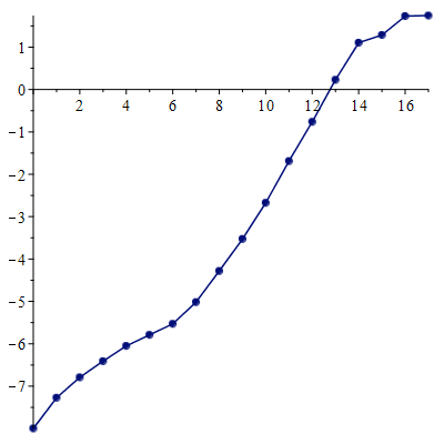
(a)

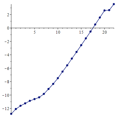
(b)

Figure 1: The plots of $\log_{10}(\varepsilon_{j})$ for (a) $N=129$ and (b) $N=2049$.

The following figures (Figures 2– 8) illustrate the reconstruction of Section 2. The preimages $v$ considered in the present paper are rather simple: the sum of characteristic functions of two or three disjoint objects at distance significantly less than $\pi/r\approx 0.314$. Most importantly, for all given examples, a proper choice of the regularisation parameter $n$ leads to super-resolution, that is in this case, allowing to separate the two objects of the preimage. We also obtain smaller relative errors $\mathfrak{E}$ in $\mathcal{L}^{2}$-norm than the naive reconstruction based on formula (1.3) in both Fourier domain and spatial domain; see (2.14) for the definition of $\mathfrak{E}$.

In this section, we abbreviate the notation $\tilde{\varPhi}_{n}[w]$ used in (2.11) and (2.12) as follows:

$$\tilde{v}_{n}:=\tilde{\varPhi}_{n}[w].$$ (3.1)

Recall that $w\approx\mathcal{F}[v]|_{B_{r}}$ is the data of Problem 1.1 and $\tilde{\varPhi}_{n}[\cdot]$ denotes the numerical PSWF reconstruction via formulas (1.4), (2.1), (2.2), and (2.4).

Figure 2 shows our PSWF reconstructions $\tilde{v}_{n}$ with $n=n^{*}$ defined by (2.11) from noiseless data $w$, in comparison with preimage $v$ and naive Fourier inversion $\tilde{v}_{\rm naive}$, for $d=1$, $N=129$, and $N=2049$. More precisely, the aforementioned data $w$ are noiseless on the uniform grid of $N$ points on $B_{r}$ in the Fourier domain. The most interesting point is that the reconstruction $\tilde{v}_{n}$ with $n$ taken according to the residual minimisation ($n=n^{*}$) achieve super-resolution. Indeed, the two parts of $v$ are sufficiently distinguished by $\tilde{v}_{n}$ even though the distance between the two parts is $\pi/(2r)$. The naive reconstruction $\tilde{v}_{\rm naive}$ obscures completely the presence of the two parts.

Note that even for noiseless data there still remains ”discretisation noise” which gets smaller when $N$ grows. For the example of Figure 2, it is $0.88\%$ for $N=129$ and $0.06\%$ for $N=2049$. Interestingly, the theoretical suggestion $n=n^{*}_{\alpha,\delta}$ of (2.5) is close to the residual minimisation choice $n^{*}$. Namely, $n^{*}_{\alpha,\delta}=12$ for $N=129$ and $n^{*}_{\alpha,\delta}=14$ for $N=129$, where $\alpha=0.75$ and $\delta$ corresponds to the ”discretisation noise” level.

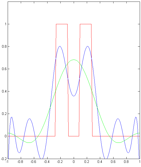
(a)

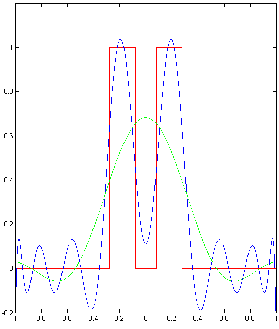
(b)

Figure 2: Reconstruction $\tilde{v}_{n}$(dark blue) using the residual minimisation from noiseless data $w$, in comparison with preimage $v$(red) and naive Fourier inversion $\tilde{v}_{\rm naive}$(green) for $d=1$. (a) $N=129$ and $n=n^{*}=12$. The relative errors: $\mathfrak{E}(\tilde{v}_{n},v)\approx 0.57$, $\mathfrak{E}(\tilde{v}_{\rm naive},v)\approx 0.71$ and $\mathfrak{E}(\tilde{\mathcal{F}}[\tilde{v}_{n}],w)\approx 4\cdot 10^{-3}$, $\mathfrak{E}(\tilde{\mathcal{F}}[\tilde{v}_{\rm naive}],w)\approx 5\cdot 10^{-2}$. (b) $N=2049$ and $n=n^{*}=16$. The relative errors: $\mathfrak{E}(\tilde{v}_{n},v)\approx 0.39$, $\mathfrak{E}(\tilde{v}_{\rm naive},v)\approx 0.67$ and $\mathfrak{E}(\tilde{\mathcal{F}}[\tilde{v}_{n}],w)\approx 4.9\cdot 10^{-9}$, $\mathfrak{E}(\tilde{\mathcal{F}}[\tilde{v}_{\rm naive}],w)\approx 5\cdot 10^{-2}$.

Figure 3 shows our PSWF reconstructions $\tilde{v}_{n}$ with $n=n_{0}$ and $n=\tilde{n}_{\varepsilon}+1$, where $n_{0}$ is defined by (2.6) and $\tilde{n}_{\varepsilon}$ is defined by (2.8) with $\varepsilon=1$, and all other parameters are the same as in Figure 2(b). Figure 3(a) demonstrates the general phenomenon that our reconstruction $\tilde{v}_{n}$ with $n=n_{0}$ behaves similarly to the naive reconstruction $\tilde{v}_{\rm naive}$. Figure 3(b) demonstrates that reconstruction $\tilde{v}_{n}$ quickly becomes unreliable after the trust criteria (2.8) is violated.

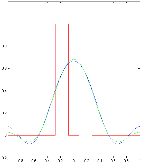
(a)

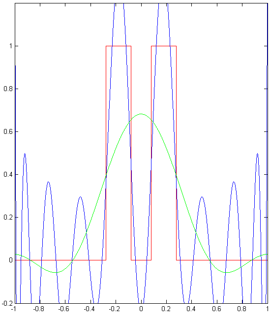
(b)

Figure 3: Reconstruction $\tilde{v}_{n}$(dark blue) from noiseless data $w$ in comparison with preimage $v$(red) and naive Fourier inversion $\tilde{v}_{\rm naive}$(green) for $d=1$ and $N=2049$: (a) $n=n_{0}=6$, (b) $n=\tilde{n}_{\varepsilon}+1=18$.

Figure 4 shows our PSWF reconstructions $\tilde{v}_{n}$ from the noisy data $w\approx\hat{v}|_{B_{r}}$ with $1.36\%$ of $\mathcal{L}^{2}$ random noise for $d=1$, $N=129$, and $n\in\left\{n^{*},n^{*}_{\varDelta},\frac{1}{2}(n^{*}+n^{*}_{\varDelta})\right\}$, where $n^{*}$, $n^{*}_{\varDelta}$ are defined by (2.11), (2.12) and $\varDelta=0.0136\|\hat{v}\|_{\mathcal{L}^{2}(B_{r})}.$ In this example, the best reconstruction in the spatial domain is achieved when $n=\frac{1}{2}(n^{*}+n^{*}_{\varDelta})$. Figure 4(c) illustrates the well-known fact that residual minimisation ($n=n^{*}$) may yield explosion in the reconstruction from noisy data. On the other hand, Morozov’s discrepancy principle ($n=n^{*}_{\varDelta}$) leads to a stable reconstruction, but, in our example, it fails to achieve super-resolution; see Figure 4(a).

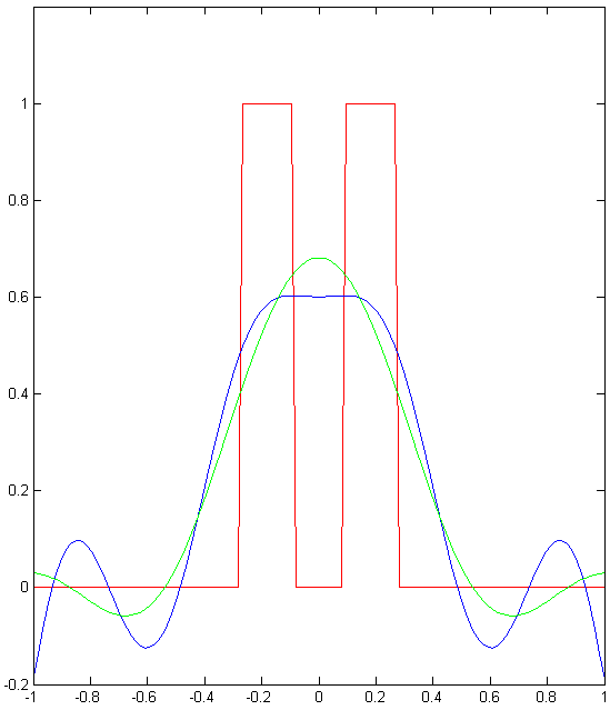
(a)

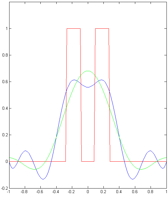
(b)

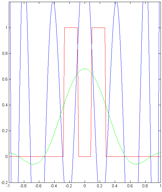
(c)

Figure 4: Reconstruction $\tilde{v}_{n}$ (dark blue) from noisy data $w$ with $1.36\%$ of $\mathcal{L}^{2}$ random noise for $d=1$ and $N=129$. The preimage $v$ and naive Fourier inversion $\tilde{v}_{\rm naive}$ are displayed similar to Figure 2. (a) The Morozov discrepancy choice $n=n_{\varDelta}^{*}=8$. The relative errors: $\mathfrak{E}(\tilde{v}_{n},v)\approx 0.69$ and $\mathfrak{E}(\tilde{\mathcal{F}}[\tilde{v}_{n}],w)\approx 0.0131$. (b) The optimal choice $n=\frac{1}{2}(n_{\varDelta}^{*}+n^{*})=10$ (best reconstruction in the spatial domain). The relative errors: $\mathfrak{E}(\tilde{v}_{n},v)\approx 0.66$ and $\mathfrak{E}(\tilde{\mathcal{F}}[\tilde{v}_{n}],w)\approx 0.0130$. (c) The residual minimisation choice $n=n^{*}=12$. The relative errors: $\mathfrak{E}(\tilde{v}_{n},v)\approx 2.62$, and $\mathfrak{E}(\tilde{\mathcal{F}}[\tilde{v}_{n}],w)\approx 0.0129$.

Figure 5 and Figure 6 show our PSWF reconstruction $\tilde{v}_{n}$ with $n=n^{*}$ defined by (2.11) from noiseless data $w$, in comparison with preimage $v$ and naive Fourier inversion $\tilde{v}_{\rm naive}$ for $d=2$ and $N=129$. In addition, we implement $\mathcal{R}^{-1}$ using the filtered back projection (FBP) algorithm with the angle step of $2.5^{\circ}$. Similarly to the one-dimensional example of Figure 2, the reconstruction $\tilde{v}_{n}$ with $n$ taken according to the residual minimisation ($n=n^{*}$) achieves super-resolution. Indeed, the distances between the three square parts of $v$ are significantly less than $\pi/r$: two bottom squares are at the distance $0.1$, while the top square and any of the bottom squares are at the distance $0.05$. Nevertheless, the three parts of $v$ are sufficiently distinguished by $\tilde{v}_{n}$. The naive reconstruction $\tilde{v}_{\rm naive}$ obscures completely the presence of the three parts.

Figure 5: Reconstruction $\tilde{v}_{n}$(middle) using the residual minimisation from noiseless data $w$ in comparison with preimage $v$(left) and naive Fourier inversion $\tilde{v}_{\rm naive}$(right) for $d=2$, $N=129$, $n=n^{*}=9$. The relative errors: $\mathfrak{E}(\tilde{v}_{n},v)\approx 0.54$, $\mathfrak{E}(\tilde{v}_{\rm naive},v)\approx 0.60$ and $\mathfrak{E}(\tilde{\mathcal{F}}[\tilde{v}_{n}],w)\approx 0.09$, $\mathfrak{E}(\tilde{\mathcal{F}}[\tilde{v}_{\rm naive}],w)\approx 0.11$.

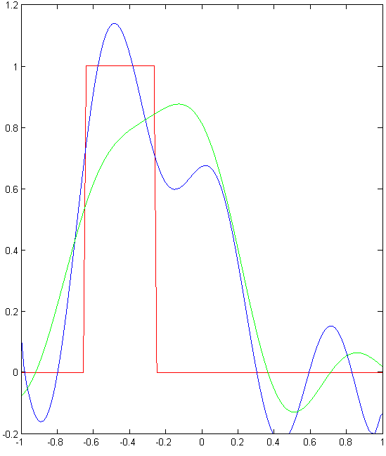
(a)

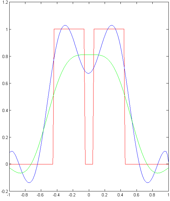
(b)

Figure 6: Cross-sections of reconstruction $\tilde{v}_{n}$(dark blue) of Figure 5, in comparison with preimage $v$(red) and naive Fourier inversion $\tilde{v}_{\rm naive}$(green): (a) along the $y$-axis ($x=0$); (b) along the $x$-axis ($y=0$).

Figure 8 shows our PSWF reconstruction $\tilde{v}_{n}$ with $n=n^{*}$ defined by (2.11) from noisy data $w\approx\hat{v}|_{B_{r}}$ with $21\%$ of $\mathcal{L}^{2}$ random noise in comparison with preimage $v$ and naive Fourier inversion $\tilde{v}_{\rm naive}$ for $d=2$ and $N=129$. In addition, Figure 7 illustrates the noiseless data $\hat{v}|_{B_{r}}$ and the noisy data $w$. In contrast to the one-dimensional example of Figure 4, the reconstruction $\tilde{v}_{n}$ with $n$ taken according to the residual minimisation ($n=n^{*}$) works as well as for the noiseless case shown in Figure 5. Most importantly, this reconstruction $\tilde{v}_{n}$ is rather stable and gives super-resolution even for a considerable level of noise.

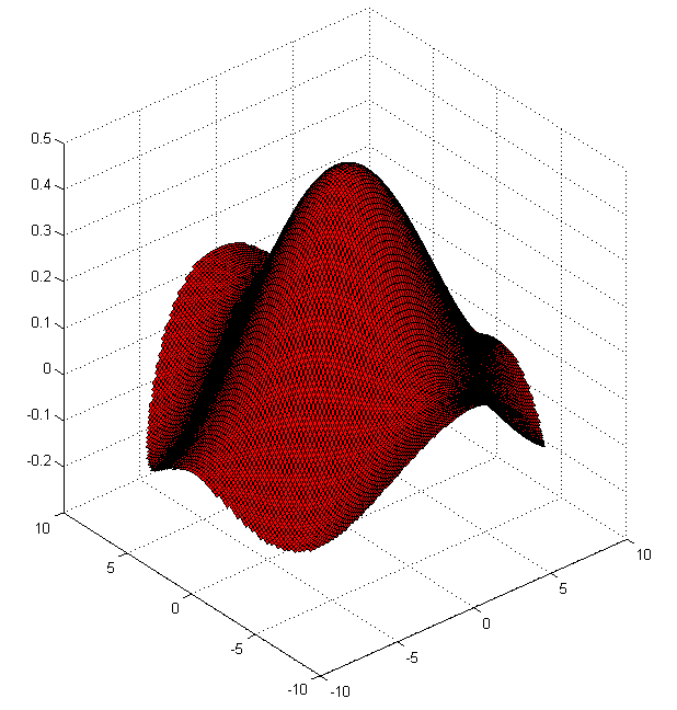
(a)

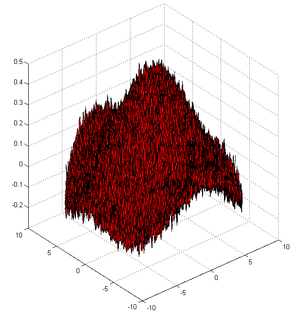
(b)

Figure 7: The noisy data $w$ with $21\%$ of random $\mathcal{L}^{2}$ noise in comparison with the noiseless data $\hat{v}|_{B_{r}}$ for the preimage $v$ displayed left on Figure 5 : (a) the real part of $\hat{v}|_{B_{r}}$; (b) the real part of $w\approx\hat{v}|_{B_{r}}$.

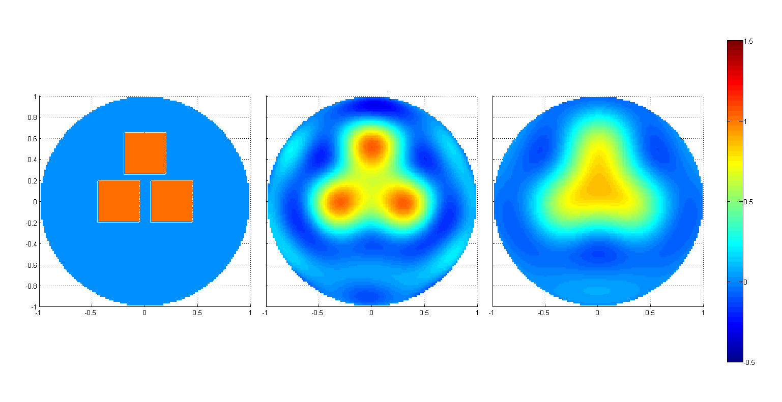
Figure 8: Reconstruction $\tilde{v}_{n}$(middle) using the residual minimisation from thenoisy data displayed on Figure 7(b) in comparison with preimage $v$(left) and naive Fourier inversion $\tilde{v}_{\rm naive}$(right) for $d=2$, $N=129$, $n=n^{*}=8$. The relative errors: $\mathfrak{E}(\tilde{v}_{n},v)\approx 0.55$, $\mathfrak{E}(\tilde{v}_{\rm naive},v)\approx 0.60$ and $\mathfrak{E}(\tilde{\mathcal{F}}[\tilde{v}_{n}],w)\approx 0.23$, $\mathfrak{E}(\tilde{\mathcal{F}}[\tilde{v}_{\rm naive}],w)\approx 0.24$.

4 Conclusion

We implemented numerically formulas of [16] for finding a compactly supported function $v$ on ${\mathbb{R}}^{d}$, $d\geq 1$, from its Fourier transform $\mathcal{F}[v]$ given within the ball $B_{r}$ (that is, for Problem 1.1). Our approach is based on theoretical and numerical results on the prolate spheroidal wave functions, the Radon transform, and regularisation methods. The present work demonstrates the numerical efficiency of this approach to Problem 1.1 in its general setting; including the following points.

• In spite of the exponential instability of the problem, we achieved super-resolution even for noisy data by appropriate choice of the regularisation parameter $n$. In particular, for $d\geq 2$, the approach works well even for a considerable level of random noise.

• Our reconstruction (with appropriate choice of $n$) gives smaller errors in $\mathcal{L}^{2}$-norm (in both Fourier domain and spatial domain) than the conventional reconstruction based on formula (1.3).

• Our reconstruction with $n=n_{0}:=\left\lfloor\lower 0.6458pt\hbox{\large$\textstyle\frac{2c}{\pi}$}\right\rfloor$ behaves similarly to the conventional reconstruction based on formula (1.3). In our examples, taking $n$ larger than $n_{0}$ gives better results.

We expect that similar numerical behaviour (in particular, super-resolution) is also possible for monochromatic inverse scattering (considered, for example, in [2, 4, 10, 12, 13, 21]) and for other generalisations of Problem 1.1.

5 Acknowledgements

The work was initiated in the framework of the internship of G.V. Sabinin at the Centre de Mathématique Appliquées of Ecole Polytechnique under the supervision of R.G. Novikov in August-October 2021.

References

- [1] R. Adelman, N.A. Gumerov, R. Duraiswami, Software for computing the spheroidal wave functions using arbitrary precision arithmetic, arXiv:1408.0074.
- [2] N.V. Alexeenko, V.A. Burov, O.D. Rumyantseva, Solution of the three-dimensional acoustical inverse scattering problem. The modified Novikov algorithm, Acoustical Physics 54(3) (2008), 407–419.
- [3] N. Alibaud, P. Maréchal, Y. Saesor, A variational approach to the inversion of truncated Fourier operators. Inverse Problems, 25(4) (2009), 045002.
- [4] V.A. Burov, N.V. Alekseenko, O.D. Rumyantseva, Multifrequency generalization of the Novikov algorithm for the two-dimensional inverse scattering problem, Acoustical Physics 55(6) (2009), 843–856.
- [5] A. Bonami, A. Karoui, Uniform bounds of prolate spheroidal wave functions and eigenvalues decay, Comptes Rendus de l’Académie des Sciences, Series I, 352(3) (2014), 229–234.
- [6] A. Bonami, A. Karoui, Spectral decay of time and frequency limiting operator, Applied and Computational Harmonic Analysis 42(1) (2017), 1–20.
- [7] G. Beylkin, L. Monzón, Nonlinear inversion of a band-limited Fourier transform, Applied and Computational Harmonic Analysis, 27(3) (2009), 351–366.
- [8] E. J. Candès, C. Fernandez-Granda, Towards a mathematical theory of super-resolution, Communications on Pure and Applied Mathematics, 67 (2014), 906–956.
- [9] R.W. Gerchberg, Superresolution through error energy reduction, Optica Acta: International Journal of Optics, 21(9) (1974), 709–720.
- [10] P. Hähner, T. Hohage, New stability estimates for the inverse acoustic inhomogeneous medium problem and applications, SIAM Journal on Mathematical Analysis, 33(3) (2001), 670–685.
- [11] H.A. Hasanov, V.G. Romanov, Introduction to inverse problems for differential equations. Second edition, Springer (2021), 515 pp.
- [12] T. Hohage, F. Weidling, Variational source conditions and stability estimates for inverse electromagnetic medium scattering problems, Inverse Problems and Imaging, 11(1) (2017), 203–220.
- [13] M. Isaev, R.G. Novikov, New global stability estimates for monochromatic inverse acoustic scattering, SIAM Journal on Mathematical Analysis, 45(3) (2013), 1495–1504.
- [14] M. Isaev, R.G. Novikov, Hölder-logarithmic stability in Fourier synthesis, Inverse Problems 36(12) (2020), 125003.
- [15] M. Isaev, R.G. Novikov, Stability estimates for reconstruction from the Fourier transform on the ball, Journal of Inverse and Ill-posed Problems, 29(3) (2021), 421–433.
- [16] M. Isaev, R.G. Novikov Reconstruction from the Fourier transform on the ball via prolate spheroidal wave functions, arXiv:2107.07882.
- [17] S. Karnik, J. Romberg, M. A. Davenport, Improved bounds for the eigenvalues of prolate spheroidal wave functions and discrete prolate spheroidal sequences. Applied and Computational Harmonic Analysis 55(1) (2021), 97–128.
- [18] A. Lannes, S. Roques, M.-J. Casanove, Stabilized reconstruction in signal and image processing: I. partial deconvolution and spectral extrapolation with limited field. Journal of modern Optics, 34(2) (1987), 161–226.
- [19] F. Natterer, The Mathematics of Computerized Tomography. Society for Industrial Mathematics, (2001), 184 pp.
- [20] A. Papoulis, A new algorithm in spectral analysis and band-limited extrapolation. IEEE Transactions on Circuits and Systems, 22(9) (1975), 735–742.
- [21] A.S. Shurup, Numerical comparison of iterative and functional-analytic algorithms for inverse acoustic scattering, Eurasian Journal of Mathematical and Computer Applications 10(1) (2022); e-preprint arXiv:2201.04542.
- [22] D. Slepian, Some comments on Fourier analysis, uncertainty and modeling, SIAM Review, 25(3) (1983), 379–393.
- [23] A.N. Tikhonov, V. Y. Arsenin, Solutions of ill-posed problems. Washington : New York : Winston ; distributed solely by Halsted Press, (1977), 258 p.
- [24] L. L. Wang, Analysis of spectral approximations using prolate spheroidal wave functions. Mathematics of Computation 79 (2010), no. 270, 807–827.
- [25] H. Xiao, V. Rokhlin, N. Yarvin, Prolate spheroidal wavefunctions, quadrature and interpolation. Inverse Problems 17(4) (2001), 805–838.