Distinguishing two dark matter component particles at $e^{+}e^{-}$ colliders

Abstract

We investigate ways of identifying two kinds of dark matter (DM) component particles at high-energy colliders. The strategy is to notice and distinguish double-peaks(humps) in the missing energy/transverse energy distribution. The relative advantage of looking for missing energy is pointed out, in view of the fact that the longitudinal component of the momentum imbalance becomes an added input. It thus turns out that an electron-positron collider is better suited for discovering a two-component DM scenario, so long as both of the components are kinematically accessible. This and a number of associated conclusions are established, using for illustration a scenario including a scalar and a spin-1/2 particle. We also formulate a set of measurable quantities which quantify the distinguishability of the two humps, defined in terms of double-Gaussian fits to the missing energy distribution. The efficacy of these variables in various regions of the parameter space is discussed, using the aforesaid model as illustration.

1 Introduction

Evidence for dark matter (DM) has accumulated from different astrophysical observations like rotation curves of galaxies Rubin:1970zza ; Zwicky:1937zza , gravitational lensing effects around bullet clusters Hayashi:2006kw , and cosmological observations like the anisotropy of cosmic microwave background radiation (CMBR) Hu:2001bc in WMAP Hinshaw:2012aka ; Spergel:2006hy or PLANCK Planck:2018vyg data. Observations further suggest that DM constitutes a large portion $(\simeq 24\%)$ of the energy budget of the universe, often expressed in terms of relic density $\Omega h^{2}\simeq 0.12$ Planck:2018vyg , where $\Omega={\rho}/{\rho_{c}}$ represents the cosmological density with $\rho$ being the DM density, $\rho_{c}$ the critical density and $h$ represents Hubble expansion rate in units of 100 km/s/Mpc. However, direct evidence of DM in reproducible terrestrial observations is yet to be found. We are thus still unable to confirm whether DM consists of elementary particles of the weakly or feebly interacting types. All one can say with certainty is that neutrinos cannot be the dominant components of DM, and thus physics beyond the standard model (SM) have to be there if particle DM exists.

Two major classes of ideas, both of which can account for correct relic density, are often discussed. The first category consists of weakly interacting massive particle (WIMP) scenarios where the DM particles were in thermal and chemical equilibrium in early universe, and have frozen out when their annihilation rate dropped below the Hubble expansion rate Bertone:2004pz ; Roszkowski:2017nbc ; Kolb:1990vq . In the second category, one can have feebly interacting massive particles (FIMP)Hall:2009bx which do not thermalise with the cosmic bath, and are presumably produced from the decay or scattering of some massive particles in thermal bath. We shall be concerned here with WIMPs, since they are the likeliest one to be detected in collider experiments which constitute the theme of this paper.

It is of course possible to have more than one DM components simultaneously, and this is the possibility we are concerned with. While many of the existing multicomponent DM studies are in the context of WIMPs Aoki:2012ub ; Liu:2011aa ; Cao:2007fy ; Bhattacharya:2013hva ; Esch:2014jpa ; Karam:2016rsz ; Ahmed:2017dbb ; Poulin:2018kap ; Aoki:2018gjf ; YaserAyazi:2018lrv ; Aoki:2017eqn ; Biswas:2013nn ; Bhattacharya:2016ysw ; Bhattacharya:2017fid ; Barman:2018esi ; Bhattacharya:2018cgx ; Bhattacharya:2019fgs ; Borah:2019aeq ; Chakraborti:2018lso ; Chakraborti:2018aae ; Bhattacharya:2018cqu ; Yaguna:2021rds ; Belanger:2021lwd ; VanLoi:2021dzv ; Yaguna:2021vhb ; DiazSaez:2021pfw ; Chakrabarty:2021kmr ; Nam:2020twn ; Betancur:2020fdl ; Nanda:2019nqy ; Bhattacharya:2019tqq ; Elahi:2019jeo ; Herrero-Garcia:2018lga ; Das:2022oyx , scenarios with more than one DM types have also been studied Bhattacharya:2021rwh ; DuttaBanik:2016jzv ; Choi:2021yps . Direct search experiments XENON:2018voc ; PandaX-4T:2021bab might probe two component WIMP frameworks via observation of a kink in the recoil energy spectrum Herrero-Garcia:2017vrl ; Herrero-Garcia:2018qnz . We devote the present discussion to the collider detectability and distinguishability of two DM components, both of whom are of the WIMP type. However, studies on collider searches are relatively fewer Hernandez-Sanchez:2020aop ; Konar:2009qr . Here we develop some criteria for the discrimination of two peaks in missing energy distributions, in an illustrative scenario where the DM components are pair-produced in cascades, along with the same kinds of visible particles.

More specifically, we consider cases where the two DM components belong to two separate ‘dark sectors’. The initial hard scattering pair-produces members of either sector, and each of these members initiate a decay chain culminating in the DM candidate of either kind. The visible particles produced alongside happen in our examples to be multileptons. Our purpose is to maximise the visibility of the two peaks, via discriminants based on their heights, separation and spreads.

We also emphasize that the main principle(s), on which our suggested method of analysis is based, do not depend on the model used here for illustration. Certain features of the model are course best suited for substantial production of the two kinds of DM particles, and the decay chains that occur here simplify and facilitate what we wish to demonstrate. More complicated avenues of DM production are of course within our horizon, but the points we make here serve as leitmotifs in any analysis.

We establish further that an electron-positron collider is in most cases better suited for thus discerning the two DM components, as compared to hadronic machines. The main reason, as we shall show, is that in electron-positron collisions, the full kinematic information, especially that on longitudinal components of momenta (including missing momenta) can be utilised. In addition, it helps the suppression of standard model (SM) backgrounds. The option of using polarised beams, too, can be of advantage.

On the whole, the essential points developed and established in this study are:

• A two-component WIMP scenario which leads to the same final state via two different kinds of cascade, can lead to double-peaks (bumps) in kinematic distributions such as missing energy.

• An $e^{+}e^{-}$ machine having the requisite kinematic reach is advantageous in this respect, since (a) it makes use of the longitudinal components of missing momenta, and (b) beam polarization can reduce backgrounds.

• A set of measurable quantities, formulated by us for this specific purpose, are useful in making the double-peaking behaviour prominent.

The paper is organised as follows. We first discuss WIMP signal at colliders in section 2 including some general aspects of kinematics in both single-and two-component DM scenarios. In section 3 we discuss the model chosen for illustration, followed by the selection of benchmark points in section 4. Section 5 contains a discussion of the signal from two-component dark sector vis-a-vis SM backgrounds, while in section 6 we analyse the predicted results in detail. Some proposed criteria for distinguishing the peaks are exemplified in section 7. We summarise and conclude in section 8. In Appendix A-E, we include some details that are omitted in the main text.

2 WIMP signal at colliders

WIMPS are produced at colliders either via electroweak hard scattering processes or in weak decays of other particles. But no component of currently designed collider detectors is equipped to register their presence. Their smoking gun signatures, therefore, result from energy/momentum imbalance in the final state, rising above SM backgrounds as well as the imbalance due to mis measurement. Such imbalance can be quantified in terms of the following kinematic variables:

• Missing Transverse Energy or MET ($\not{E}_{T}$), defined as:

  $$\not{E}_{T}=-\sqrt{(\sum_{\ell,j,\gamma}p_{x})^{2}+(\sum_{\ell,j,\gamma}p_{y})^{2}};$$ (1)

  where the sum runs over all visible objects that include leptons ($\ell$), photons ($\gamma$), jets ($j$), and also unclustered components.

• Missing Energy or ME ($\not{E}$) with respect to the centre-of-mass (CM) energy ($\sqrt{s}$), defined as:

  $$\not{E}=\sqrt{s}-\sum_{\ell,j,\gamma}E_{\rm vis}\,;$$ (2)

  where the sum runs over visible objects like $\ell,j,\gamma$ and unclustered components.

• Missing Mass or MM ($\not{M}$), defined as:

  $$\not{M}^{2}=\left(\sum_{i}p_{i}-\sum_{f}p_{f}\right)^{2}\,,$$ (3)

  which requires the knowledge of initial state four momenta ($p_{i}$) and final state ones ($p_{f}$), where $f$ runs over all the visible particles. For mono-photon process $e^{+}e^{-}\to\chi\bar{\chi}\gamma$, where $\chi(\bar{\chi})$ are DM, $\not{M}^{2}=s-2\sqrt{s}E_{\gamma}$. Here, $E_{\gamma}$ is the energy of the outgoing photon.

$\not{E}$ and $\not{M}$ are measurable in $e^{+}e^{-}$ (or $\mu^{+}\mu^{-}$) machines while hadron colliders can only measure $\not{E_{T}}$. The scalar sum of transverse momentum, sometimes referred as Effective mass ($H_{T}$) is another variable of interest for hadron colliders. $\not{E}$ or $\not{E_{T}}$ are reconstructible from the energies and momenta of visible particles, against which the DM particle(s) recoil. The resulting signals can be

$\bullet$ mono-X + $\not{E}~{}(\not{E_{T}}$), where X is a jet, a photon, a weak boson or a Higgs, or,
$\bullet$ $n$-leptons + $m$-jets + $p$ photons + $\not{E}~{}(\not{E_{T}}$)

The mono-X signature usually arises when two DM particles are produced directly via either a portal to dark sector Liew:2016oon ; Kahlhoefer:2017dnp ; Boveia:2018yeb or effective operators Abercrombie:2015wmb ; Abdallah:2015ter ; Barman:2021hhg . The kinematic observables at our disposal in such a case are the four-momentum of particle X and $\not{E_{T}}/\not{E}/\not{M}$. Among them, as we shall show from a general argument below, $\not{E}$ (whenever measurable) is likely to contain the best usable information for discriminating between two unequal-mass DM particles, both of which are produced at a collider. The longitudinal component of the momentum imbalance makes the all-important difference.

The second class of final states, namely, multi-jet/multi-lepton channels usually arises when a pair of heavy particles (usually members of the dark sector, described here as ‘Heavier Dark Sector Particles’ (HDSP)) are produced. Each of them further decays into a DM together with jets and leptons in the final state. Obviously such an event topology, with a greater multitude of visible particles, will have richer kinematics. For example, the kinematics is governed here by both the HDSP and DM masses, a phenomenon which we discuss below in detail. The resulting features of the final state play an important role in differentiating the contributions from different DM components in event distributions.

Our aim here is to investigate the correlation between $\not{E_{T}},~{}\not{E}~{}\rm{or}~{}\not{M}$ with DM mass and the mass of the HDSP, in cases where two kinds of DM particles are produced via HDSP cascades. Peaks/bumps in the distributions can be treated as tell-tale signature of multi-component DM framework, when the different bumps are distinguishable. We systematically address the issues to suggest some distinction criteria. But before we discuss some relevant features of kinematic observables for both one-and two-component WIMP scenarios.

2.1 Aspects of kinematics

We focus on multilepton/multijet final states in a scenario where the DM particles are produced at the end of decay chains in $e^{-}e^{+}$ collisions. Parameters that play decisive roles in shaping $\not{E_{T}},~{}\not{E}~{}\rm{or}~{}\not{M}$ distributions are, (a) the mass of the DM particle ($m_{\rm DM}$), and (b) its mass difference with the HDSP ($\Delta m$).

2.1.1 Single-component DM

Let us first consider a single DM with mass $m_{\rm DM}$ and an HDSP with $m_{\rm HD}=m_{\rm DM}+\Delta m$, which decays to DM with one/or more massless SM fermions. For simplicity, we assume the HDSPs are pair-produced nearly at rest, in which case, the lab frame in an $e^{+}e^{-}$ machine can be identified, approximately at least, with the rest frame of the HDSP.

The maximum $\not{E_{T}}$ is obtained when both DMs are moving in the same direction. Then (see Appendix A for details),

$$\not{E_{T}}^{max}\simeq\Delta m\left(1+r\right)\,;$$ (4)

where $r=\frac{m_{\rm DM}}{m_{\rm HD}}$ is the ratio of the DM and HDSP masses. Clearly $\not{E_{T}}^{max}$ depends on both $\Delta m$ and $m_{\rm DM}$. In order to verify that we plot $\not{E_{T}}$ distribution in Fig. 1 for inert scalar doublet model (to be discussed in detail in Sec. 3), where singly-charged scalar HDSPs are pair-produced, followed by decays to DM with on/off-shell $W^{\pm}$ bosons. The CM energy is chosen $\sqrt{s}=500(1000)$ GeV, as necessary to pair produce the HDSPs on-shell. In the plot on the left panel, we fix $r=5$ and choose different $\Delta m=\{48,98\}$ GeV, while on the right plot we fix $\Delta m=140$ GeV and choose different values of $m_{\rm DM}=\{100,350\}$ GeV. From the left plot, we see that the end-point shifts significantly towards higher value of $\not{E_{T}}$ with the increase of $\Delta m$. More importantly, the peak of the $\not{E_{T}}$ distribution also shifts to higher values with larger $\Delta m$. The plot on the right-hand side show a relatively weaker dependence on $m_{\rm DM}$. This establishes that $\not{E_{T}}$ distribution has a more pronounced dependence on $\Delta m$ than on $m_{\rm DM}$.

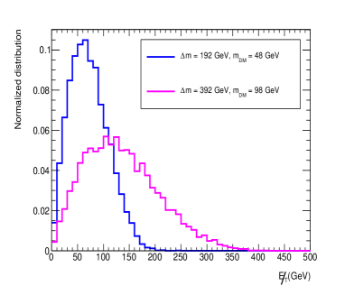
(a)

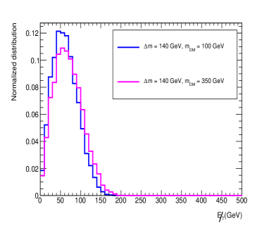
(b)

Figure 1: Normalized $\not{E_{T}}$ distribution at $e^{+}e^{-}$ collider with (a) fixed $r$, different $\Delta m$, and (b) with fixed $\Delta m$, different $m_{\rm DM}$ (see figure insets for details). We consider pair production of the singly charged scalar HDSP of an inert scalar doublet, which further decays to DM in association with on/off shell $W^{\pm}$ bosons at $\sqrt{s}=500(1000)$ GeV, as necessary to pair produce the HDSPs on-shell.

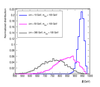
(a)

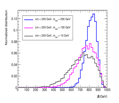
(b)

Figure 2: Normalised $\not{E}$ distribution at $e^{+}e^{-}$ collider with (a) fixed DM mass, different $\Delta m$ and with (b) fixed $\Delta m$, different DM mass (see figure insets for details). We consider pair production of singly charged scalar HDSP of an inert scalar doublet, which further decays to DM in association with on/off shell $W^{\pm}$ bosons at $\sqrt{s}=1000$ GeV.

We examine $\not{E}$ distribution next and compare with $\not{E_{T}}$ distribution. Following, ${E}_{\rm DM}=\sqrt{{|\vec{p}|^{2}_{\text{ DM}}}+m_{\rm DM}^{2}}$, an event with DM pair cascading from HDSP pair production yields,

$$\not{E}=\sqrt{{|\vec{p}_{1}|^{2}_{\text{ DM}}}+m_{\rm DM}^{2}}+\sqrt{{|\vec{p}_{2}|^{2}_{\text{ DM}}}+m_{\rm DM}^{2}}\,.$$ (5)

In order to illustrate the more noticeable presence of $m_{\rm DM}$ in $\not{E}$ distribution, as evinced from Eq. 5 , we present such distributions for different values of $\Delta m$ in Fig. 2(a), where $m_{\rm DM}$ is kept fixed. Fig. 2(b) shows similar plots with the roles of $\Delta m$ and $m_{\rm DM}$ reversed. The $\not{E}$ spectrum peak shifts to the left side with larger $\Delta m$. In Fig. 2(b), too, the $\not{E}$ distribution gets sharper with the peaks shifting to larger values with larger $m_{\rm DM}$. On the whole, the $\not{E}$ distribution, if available, is comparably sensitive to both $m_{\rm DM}$ and $\Delta m$, while $\not{E_{T}}$ is sensitive primarily to $\Delta m$. We thus conclude that an $e^{+}e^{-}$ collider is more effective in distinguishing DM components with different masses, as compared to a hadronic machine, provided that both DM components are within the kinematic reach of such a collider. $\not{M}$ distribution turns rather similar to $\not{E}$ distributions, and does not offer much advantage in our context. $\not{M}$ distributions and their comparison with $\not{E}$ are provided in Appendix A.

2.1.2 Two-component DM

We now extend the study to the two-component scenario. While the details of a two component DM model will be taken up in Section 3, here we focus on a simple situation having two scalar DM particles with masses $m_{\rm DM_{1}},m_{\rm DM_{2}}$ and mass splitting with the corresponding HDSP as ${\Delta m}_{1}~{}{\rm and}~{}{\Delta m}_{2}$ respectively. As previous, pair production of singly charged HDSPs and subsequent decay to the respective DM components with leptonically decaying on/off-shell $W^{\pm}$ is considered. Subsequent $\not{E}$ and $\not{E_{T}}$ distributions for different choices of $m_{\rm DM}$ and $\Delta m$ are studied:

• ${\Delta m}_{1}\approx{\Delta m}_{2}$ and $m_{\rm DM_{1}}<m_{\rm DM_{2}}$

  In this case, the $\not{E_{T}}$ distribution for both dark sectors is expected to merge since ${\Delta m}_{1}\approx{\Delta m}_{2}$, whereas the $\not{E}$ distributions are expected to show a double peak, owing to the dependence of $\not{E}$ on the DM mass with $m_{\rm DM_{1}}<m_{\rm DM_{2}}$. We can see this feature in Fig. 3. We assume the production cross-sections for the HDSP pairs to be equal for both the cases.

  

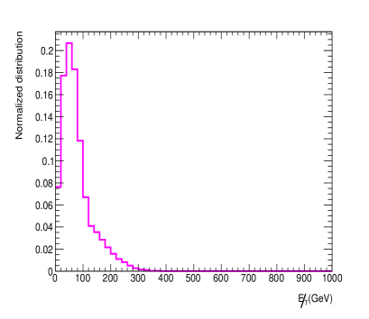
  (a)

  

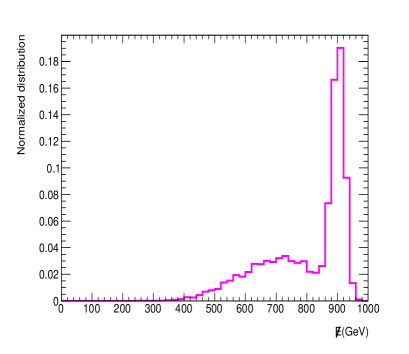
  (b)

  Figure 3: Normalized (a) $\not{E_{T}}$ and (b) $\not{E}$ distribution for two component scalar DM scenario with $\{m_{\rm DM_{1}},m_{\rm DM_{2}},{\Delta m}_{1},{\Delta m}_{2}\}=\{50,390,100,100\}$ GeV where HDSP pair production and subsequent decay chain is chosen as in Fig. 2 (see text). The production cross-sections for both the HDSP pairs are assumed equal at $\sqrt{s}=1000$ GeV.

• ${\Delta m}_{1}<{\Delta m}_{2}$ and $m_{\rm DM_{1}}\approx m_{\rm DM_{2}}$

  We consider next a scenario characterized by different mass splittings but similar DM masses. As an example, we chose $m_{\rm DM_{1}}=m_{\rm DM_{2}}=100$ GeV, ${\Delta m}_{1}=10$ GeV and ${\Delta m}_{2}=380$ GeV. Corresponding $\not{E_{T}}$ and $\not{E}$ distributions are shown in Fig. 4. The production cross-section for the lighter HDSP pair is assumed to be 50% of that of the heavier HDSP. Here the $\not{E_{T}}$ distribution shows a double-peak nature unlike the previous case, (see Fig. 4(a)), while $\not{E}$ distribution produces a better distinction where the second peak is even more prominent and well separated, see Fig. 4(b).

  

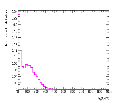
  (a)

  

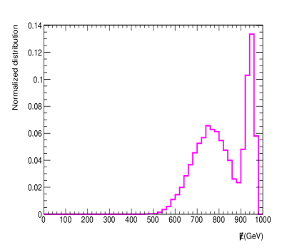
  (b)

  Figure 4: Same as Fig. 3, with $\{m_{\rm DM_{1}},m_{\rm DM_{2}},{\Delta m}_{1},{\Delta m}_{2}\}=\{100,100,10,380\}$ GeV. The production cross-section of the lighter HDSP pair is assumed half of that for the heavier HDSP pair at $\sqrt{s}=1000$ GeV.

• ${\Delta m}_{1}<{\Delta m}_{2}$ and $m_{\rm DM_{1}}<m_{\rm DM_{2}}$

  In Fig. 5 we depict a situation where both DM mass and splitting with the corresponding HDSPs are different, following a hierarchy ${\Delta m}_{1}<{\Delta m}_{2}$ and $m_{\rm DM_{1}}<m_{\rm DM_{2}}$ (see caption for model inputs). We see that the $\not{E_{T}}$ distributions (on the left) for each DM component are almost overlapping and thus show a single peak. On the other hand, $\not{E}$ distribution (on the right) shows the presence of two peaks coming from two different dark sectors. Thus, the difference in $\Delta m$ may not show up in $\not{E_{T}}$ in such cases, while $\not{E}$ still highlights it.

  

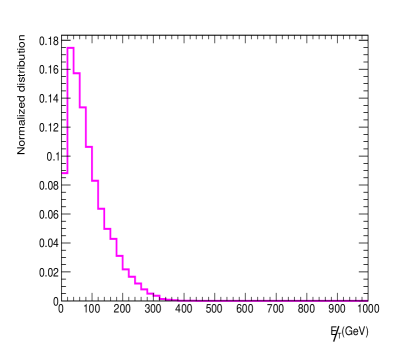
  (a)

  

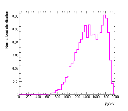
  (b)

  Figure 5: Same as Fig. 3, with $\{m_{\rm DM_{1}},m_{\rm DM_{2}},{\Delta m}_{1},{\Delta m}_{2}\}=\{50,700,100,200\}$ GeV. The production cross-sections for the heavier HDSP is assumed to be one quarter of that of the lighter ones at $\sqrt{s}=2000$ GeV.

• ${\Delta m}_{1}<{\Delta m}_{2}$ and $m_{\rm DM_{1}}>m_{\rm DM_{2}}$

  Finally we explore the possibility where the hierarchy in the DM masses is opposite to that of the mass splittings with the corresponding HDSPs as shown in Fig. 6. Again $\not{E}$ distribution (Fig. 6 (b)) shows a clear two-peak behaviour while the $\not{E_{T}}$ (Fig. 6 (a)) distribution shows a mere distortion. Note that the peak on the right side in Fig. 6 (b) corresponds to $m_{\rm DM_{1}}$, the higher DM mass.

  

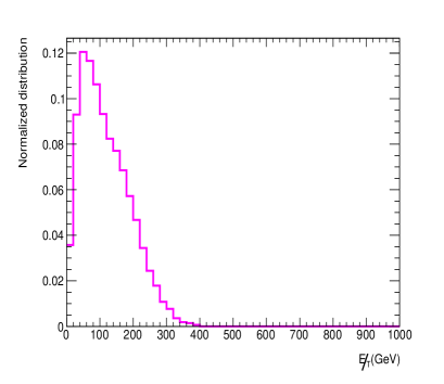
  (a)

  

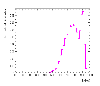
  (b)

  Figure 6: Same as Fig. 3, with $\{m_{\rm DM_{1}},m_{\rm DM_{2}},{\Delta m}_{1},{\Delta m}_{2}\}=\{390,50,100,400\}$ GeV. The production cross-sections for the heavier HDSP is taken to be one-quarter of that of the lighter ones at $\sqrt{s}=1000$ GeV.

It is clear from the preceding discussion that multipartite DM scenario can show up in terms of double peak in $\not{E}$ and/or $\not{E_{T}}$ distributions . However, $\not{E}$ is more useful as it is more sensitive to $m_{\rm DM}$ than $\not{E_{T}}$, in both the limits, $m_{\rm DM}>>\Delta m$ and $\Delta m>>m_{\rm DM}$. Complete knowledge of the total centre-of-mass energy of each collision and the very possibility of having $\not{E}$ distribution can therefore be advantageous for $e^{+}e^{-}$ collider over LHC where one has to resort to $\not{E_{T}}$, so long as DM particle productions are sufficiently copious and kinematically allowed.

So far we have discussed mainly the relative positions of the peaks. The larger is the splitting between $m_{\rm DM_{1}}$ and $m_{\rm DM_{2}}$, or ${\Delta m}_{1}$ and ${\Delta m}_{2}$, the better is the separation between the two peaks in $\not{E}$ distribution and easier it is to hint for two component DM. However, another important factor is the relative heights of the peaks, which are determined by the cross-section of the process. Two peaks of comparable size are more amenable to distinction, provided that their separation is adequate. Assuming for simplicity that the HDSPs decay into the DM candidate via a single channel with 100% branching ratio, we can estimate the size of the peaks from the pair production cross-section of the respective HDSPs. Now, HDSP production depends on its mass and thus on the parameters $m_{\rm DM}$ and $\Delta m$ (following $m_{\rm HD}=m_{\rm DM}+\Delta m$), both of which are also crucially involved in segregating the peaks in resultant $\not{E}$ (or $\not{E_{T}}$) distribution. The cross-section depends further on the model; whether the HDSPs are scalar, fermion or vector boson and what mediators contribute to the production process. We will refer to these features quantitatively when we encounter the model. We must note here that HDSP production cross-section diminishes with larger $m_{\rm DM}$ and $\Delta m$, so whichever component is heavier contributes with a smaller cross-section at least kinematically. So, the suitable scenario for discriminating DM components occurs when we do not lose cross-section significantly due to kinematics. This is better addressed if one dark sector is fermionic, while the other is scalar, as the fermion production cross-section is larger than that of a scalar with similar mass. We therefore consider HDSPs in the form of singly charged scalars ($\phi^{\pm}$) and singly charged fermions ($\psi^{\pm}$) and their subsequent decays to respective DM components at $e^{+}e^{-}$ collider. We shall examine in specific how they can yield distinguishable peaks in $\not{E}$ ($\not{E_{T}}$) distributions with comparable cross-sections after satisfying cosmological constraints, in context of an illustrative model, which we elaborate next.

3 A model with two DM components

We illustrate our numerical results in terms of a model which consists of two dark sectors having two stable DM candidates: $(i)$ Scalar DM (SDM), as the lightest neutral state of an inert scalar doublet $\Phi^{T}_{i}=\left(\begin{matrix}\phi^{+}&&\frac{\phi^{0}+iA^{0}}{\sqrt{2}}\end{matrix}\right)$ and $(ii)$ Fermion DM (FDM), the lightest neutral state that arises from an admixture of a vectorlike fermion doublet $\Psi^{T}=\left(\begin{matrix}\psi&&\psi^{-}\end{matrix}\right)$ and a right handed (RH) fermion singlet $\chi_{R}$. Stability of both DM components is ensured by additional ${\mathcal{Z}_{2}\otimes\mathcal{Z}^{\prime}_{2}}$ symmetry, where the inert scalar doublet transforms under $\mathcal{Z}_{2}$, while the fermion fields transform under a different discrete symmetry, namely, $\mathcal{Z}^{\prime}_{2}$. The quantum numbers of additional fields are shown in the Table 1. The minimal renormalizable Lagrangian for this model then reads,

$$\mathcal{L}\supset\mathcal{L}^{\rm SDM}+\mathcal{L}^{\rm FDM}.$$ (6)

Fields		$\underbrace{SU(3)_{C}\otimes SU(2)_{L}\otimes U(1)_{Y}}$ $\otimes\underbrace{\mathcal{Z}_{2}\otimes\mathcal{Z}^{\prime}_{2}}$
SDM	$\Phi=\left(\begin{matrix}\phi^{+}\\ \frac{1}{\sqrt{2}}(\phi^{0}+iA^{0})\end{matrix}\right)$	1            2          1           -     +
FDM	$\Psi_{L,R}=\left(\begin{matrix}\psi\\ \psi^{-}\end{matrix}\right)_{L,R}$	1            2          -1          +     -
	$\chi_{{}_{R}}$	1            1          0          +     -

Table 1: Charge assignment of the BSM fields under the gauge group $\mathcal{G}\equiv\mathcal{G}_{\rm SM}\otimes\mathcal{G}_{\rm DM}$ in the toy scenario. Here $\mathcal{G}_{\rm SM}\equiv SU(3)_{C}\otimes SU(2)_{L}\otimes U(1)_{Y}$ and $\mathcal{G}_{\rm DM}\equiv\mathcal{Z}_{2}\otimes\mathcal{Z}^{\prime}_{2}$.

The Lagrangian for the SDM sector, having inert scalar doublet $\Phi$ can be written as :

$$\mathcal{L}^{\rm SDM} = \Big{|}\Big{(}\partial^{\mu}-ig_{2}\frac{\sigma^{a}}{2}{W^{a}}^{\mu}-ig_{1}\frac{Y}{2}B^{\mu}\Big{)}{\Phi}\Big{|}^{2}-V(\Phi,H)\,;$$

$$V(\Phi,H) = \mu_{\Phi}^{2}(\Phi^{\dagger}\Phi)+\lambda_{\Phi}(\Phi^{\dagger}\Phi)^{2}+\lambda_{1}(H^{\dagger}H)(\Phi^{\dagger}\Phi)+\lambda_{2}(H^{\dagger}\Phi)(\Phi^{\dagger}H)+\frac{\lambda_{3}}{2}[(H^{\dagger}\Phi)^{2}+h.c.]~{}\,.$$

Note that we assume $\mu_{\Phi}^{2}>0$ which keep vacuum extension value (vev) $\langle\Phi\rangle=0$ and ensure $\mathcal{Z}_{2}$ remains unbroken. $H$ represents SM Higgs isodoublet. After Electroweak Symmetry Breaking (EWSB), the SM Higgs acquires non zero vev, $\langle H\rangle=v~{}(246~{}{\rm GeV})$ and generates physical states in the form of CP even state $\phi^{0}$ (mass $m_{\phi^{0}}$), CP-odd state $A^{0}$ (mass $m_{A^{0}}$) and charged scalar states $\phi^{\pm}$ (mass $m_{\phi^{\pm}}$) with adequate mass splitting between them. Using minimization conditions of the scalar potential $V(H,\Phi)$ along different field directions and the definitions of physical states, one can obtain the following relations between the mass eigenvalues and parameters involved in the scalar potential (for details, see Dolle:2009fn ; Bhattacharya:2019fgs ):

$$\mu_{H}^{2}~{}=~{}\frac{m_{h}^{2}}{2},~{}~{}~{}~{}\mu_{\Phi}^{2}~{}=~{}m_{\phi^{0}}^{2}-\lambda_{L}v^{2},~{}~{}\lambda_{1}~{}=~{}2\lambda_{L}-\frac{2}{v^{2}}(m_{\phi^{0}}^{2}-m_{\phi^{\pm}}^{2})~{},$$

$$\lambda_{2}~{}=~{}\frac{1}{v^{2}}(m_{\phi^{0}}^{2}+m_{A^{0}}^{2}-2m_{\phi^{\pm}}^{2})~{}~{}{\rm{and}}~{}\lambda_{3}~{}=~{}\frac{1}{v^{2}}(m_{\phi^{0}}^{2}-m_{A^{0}}^{2})~{}~{};$$ (8)

where $\lambda_{L}=\frac{1}{2}(\lambda_{1}+\lambda_{2}+\lambda_{3})$ and $m_{h}$ represents the mass of SM-like neutral scalar found at LHC with $m_{h}=125.09$ GeV. In our analysis we consider the mass hierarchy: $m_{\phi^{0}}<m_{A^{0}},m_{\phi^{\pm}}$ and hence the lightest neutral state $\phi^{0}$ with mass $m_{\phi^{0}}$ is a viable DM candidate. The parameters relevant for DM phenomenology from SDM sector are given by:

$$\{m_{\rm DM_{1}},~{}\Delta m_{1},~{}\lambda_{L}\}.$$ (9)

Here $m_{\rm DM_{1}}=m_{\phi^{0}},~{}\Delta m_{1}=m_{\phi^{\pm}}-m_{\phi^{0}}\simeq m_{A^{0}}-m_{\phi^{0}}$, assuming $m_{\phi^{\pm}}\simeq m_{A^{0}}$, which does not alter subsequent DM phenomenology or collider analysis significantly.

Let us now turn to FDM sector. The minimal renormalizable Lagrangian for FDM having one vector-like doublet ($\Psi$) and one right-handed singlet ($\chi_{R}$) reads Dutta:2020xwn :

$$\mathcal{L}^{\rm FDM} = \overline{\Psi}_{L(R)}~{}[i\gamma^{\mu}(\partial_{\mu}-ig_{2}\frac{\sigma^{a}}{2}W_{\mu}^{a}-ig_{1}\frac{Y^{\prime}}{2}B_{\mu})]~{}\Psi_{L(R)}+\overline{\chi_{{}_{R}}}~{}(i\gamma^{\mu}\partial_{\mu})~{}\chi_{{}_{R}}$$ (10)

$$- m_{\psi}\overline{\Psi}\Psi-\Big{(}\frac{1}{2}m_{\chi}\overline{\chi_{{}_{R}}}(\chi_{{}_{R}})^{c}+h.c\Big{)}-\frac{Y}{\sqrt{2}}\Big{(}~{}\overline{\Psi_{L}}~{}\widetilde{H}{\chi_{R}}+~{}\overline{\Psi_{R}}~{}\widetilde{H}{\chi_{R}}^{c}+h.c\Big{)}\,;$$

where $\Psi_{L(R)}=P_{L(R)}\Psi;~{}P_{L/R}=\frac{1}{2}(1\mp\gamma_{5})$. After EWSB, the neutral component of the doublet $\Psi$ mixes with the neutral singlet $\chi_{R}$ via the Yukawa coupling $Y$. The resulting mass matrix in the basis of $({\psi_{R}}^{c},\psi_{L},{\chi_{{}_{R}}}^{c})^{T}$ is given by:

$$\mathcal{M}=\left(\begin{array}[]{ccc}0&m_{\psi}&\frac{Yv}{2}\\ m_{\psi}&0&\frac{Yv}{2}\\ \frac{Yv}{2}&\frac{Yv}{2}&m_{\chi}\\ \end{array}\right)\,,$$ (11)

where $v=\langle H\rangle~{}(246~{}{\rm GeV})$ is the vacuum expectation value (vev) of the SM Higgs. Upon diagonalisation by a unitary matrix, the mass eigenvalues of the physical states are:

$$m_{\psi_{{}_{1}}} = m_{\chi}\cos^{2}\theta+m_{\psi}\sin^{2}\theta-\frac{Yv}{\sqrt{2}}\sin 2\theta,$$

$$m_{\psi_{{}_{2}}} = m_{\psi},$$ (12)

$$m_{\psi_{{}_{3}}} = m_{\psi}\cos^{2}\theta+m_{\chi}\sin^{2}\theta+\frac{Yv}{\sqrt{2}}\sin 2\theta,$$

$$m_{\psi^{\pm}} = m_{\psi}~{};$$

where $\theta$ denotes singlet-doublet mixing angle; in terms of model parameters, it is given by:

$$\tan 2\theta=\frac{Yv}{\sqrt{2}(m_{\psi}-m_{\chi})}\,.$$ (13)

For $Yv/\sqrt{2}<m_{\chi}\ll m_{\psi}$, $m_{\psi_{{}_{3}}}>m_{\psi_{{}_{2}}}(\equiv m_{\psi^{\pm}})>m_{\psi_{{}_{1}}}$ makes $\psi_{{}_{1}}$ the DM. Note here all the neutral states, $\psi_{1,2,3}$ are Majorana fermions. The phenomenology of FDM mainly depends on the following independent parameters:

$$\{m_{\rm DM_{2}},~{}\Delta m_{2},~{}\sin\theta\}\,;$$ (14)

where $m_{\rm DM_{2}}=m_{\psi_{1}},\Delta m_{2}=m_{\psi^{\pm}}-m_{\psi_{1}}=m_{\psi_{2}}-m_{\psi_{1}}$. In terms of these parameters,

$$Y = \frac{\sqrt{2}~{}\Delta m_{2}~{}\sin 2\theta}{v}\,,$$

$$m_{\psi} = m_{\psi_{1}}\sin^{2}\theta+m_{\psi_{3}}\cos^{2}\theta\,,$$ (15)

$$m_{\chi} = m_{\psi_{1}}\cos^{2}\theta+m_{\psi_{3}}\sin^{2}\theta.$$

The dependence of $Y$ on $\Delta m_{2}$ as well as $\theta$ plays an important role in the consequent FDM phenomenology. We note further that the two dark sectors have no renormalizable interaction term, so that DM-DM conversions occur mainly via Higgs portal coupling.

3.1 Constraints on the model parameters

The parameters of the model are subject to the following constraints, which we abide by:

• A stable vacuum at the electroweak scale Kannike:2012pe ; Chakrabortty:2013mha is ensured by,

  $$\lambda_{H},\,\lambda_{\Phi}>0\,;~{}\lambda_{1}+2\sqrt{\lambda_{H}\lambda_{\Phi}}>0\,;~{}\lambda_{1}+\lambda_{2}-|\lambda_{3}|+2\sqrt{\lambda_{H}\lambda_{\Phi}}>0\,.$$ (16)

• Perturbativity at the electroweak scale requires,

  $$|\lambda_{H}|<{4\pi}~{};~{}~{}|\lambda_{\Phi}|<{4\pi}~{};~{}|\lambda_{1,2,3}|<{4\pi}~{}~{}{\rm and}~{}~{}|Y|<\sqrt{4\pi}~{}.$$ (17)

• Limits on the masses from non-observation of the BSM particles at collider search, the most significant of those here are $m_{\chi^{\pm}}>102.7$ GeV LEP and $m_{\phi^{\pm}}>70$ GeV Pierce:2007ut .

• The requirement that the two DM components $\phi^{0}$ and $\psi_{1}$ saturate the relic-density according to the Planck data Planck:2018vyg at $2\sigma$ level,

  $$\Omega_{\rm DM}h^{2}=\Omega_{\rm DM_{1}}h^{2}+\Omega_{\rm DM_{2}}h^{2}=\Omega_{\phi^{0}}h^{2}+\Omega_{\psi_{1}}h^{2}\equiv 0.12\pm 0.001.$$ (18)

• Limit on spin independent DM-nucleon cross-section from non-observation of WIMP in direct search experiments, the latest being XENON-1T, at $2\sigma$ level XENON:2018voc ; PandaX-4T:2021bab provides

  $$\sigma^{SI}_{\rm{min}}\lesssim 10^{-47}~{}{\rm{cm}^{2}}.$$ (19)

We focus mainly on the DM constraints and demonstrate the allowed parameter space of the model, which in turn provides some characteristic benchmark points that is taken up for subsequent collider analysis.

Dark matter constraints The most important constraint comes from the DM relic density, where individual densities ($\Omega_{\rm DM_{i}}(i=1,2)$) add to the total observed relic as dictated by PLANCK data Planck:2018vyg . We may further recall that relic (over/under) abundance of a particular WIMP is inversely proportional to the thermal average of its annihilation cross-section to visible sector particles as well as to other DMs,

$$\Omega_{\rm DM_{i}}\sim\frac{1}{\langle\sigma v\rangle_{i}}\,.$$ (20)

Now, one may assume that the DM number density of any component around the earth is proportional to the share of that component in the total relic density. In such a situation, the upper limit on the scattering cross-section of the $i$th DM component ($\sigma_{i}^{\rm{eff}}$) with the detector nucleon for direct search is related to $\sigma_{i}$, the cross-section if the corresponding component were the sole WIMP DM constituent, by the fraction of relic density with which it is present in a two component set up, following Bhattacharya:2016ysw ,

$$\sigma_{i}^{\rm{eff}}={\frac{\Omega_{\rm{DM_{i}}}}{\Omega_{\rm{DM}}}}\sigma_{i}\,.$$ (21)

Thus the direct search limit on a DM component is different from the case where it is the only WIMP candidate. Since any WIMP is subject to both the limits from relic density and direct search, it is useful to note two more points. First, the tension between the limit on the cross-section in direct searches and the relic density limit is relaxed in scenarios where the dark sector permits co-annihilation, as occurs for both the SDM and FDM components of our illustrative model. Secondly, the right-chiral fermion $\chi_{R}$ in FDM has no Z-coupling (having $Q=Y=0$), its mixing with $\psi_{0}$ suppresses the Z-induced contribution to the elastic scattering and relieves the pressure from direct search limits. Annihilation, co-annihilation and conversion processes for both DM components of the model are mentioned in Appendix B.

In order to find the consistent DM parameter space, we implement the model in Feynrules Degrande:2011ua and in MicrOmegas Belanger:2018ccd to perform a numerical scan on the relevant parameters in the following range:

$$30~{}\leq m_{\phi^{0}}\leq 600~{}{\rm GeV},~{}1~{}\leq\Delta m_{1}\leq 500~{}{\rm GeV},~{}0.01~{}\leq\lambda_{L}\leq 0.1,$$

$$30\leq~{}m_{\psi_{1}}\leq 600~{}\rm GeV,~{}1~{}\leq\Delta m_{2}\leq 500~{}{\rm GeV},~{}0.01~{}\leq\sin\theta\leq 0.3~{}.$$ (22)

We present in Fig. 7, the allowed region of the model in the planes of (a) $m_{\rm DM_{1}}-\Delta m_{1}$ and (b) $m_{\rm DM_{2}}-\Delta m_{2}$. Red points satisfy relic density and the blue points satisfy additionally the direct search bound from XENON1T. It is seen that for the scalar DM, relic (under)abundance and direct detection constraints are both satisfied for almost the entire range of $m_{\rm DM_{1}},~{}\Delta m_{1}$ scanned here. This is achieved mainly due to two reasons: one, the gauge mediated depletion processes (see Appendix B for details) ensure significant annihilation cross-section, while suitable choice of the parameter $\lambda_{L}$, which governs the interaction between the DM and SM Higgs, ensures the consistency with direct detection bound. For FDM case (see Fig. 7(b)), both relic density and direct search constraints are satisfied consistently for $\Delta m_{2}\lesssim 20$ GeV. This is due to co-annihilation processes contributing significantly to relic density with smaller $\Delta m_{2}$, which do not contribute to DM elastic scattering for direct search. We also note that for $m_{\psi_{1}}\simeq\frac{m_{h}}{2}$, in the Higgs resonance region, one can only simultaneously satisfy both relic (under) abundance and direct detection constraints even for larger $\Delta m_{2}$, where the co annihilation contribution is compensated by resonant enhancement. We further note that there are two white regions in Fig. 7(b), where the relic density constraints can not be satisfied. For $\Delta m_{2}\simeq 20-100$ GeV, the co-annihilation contribution turns drastically low, subject to the range of $\sin\theta$ used for the scan, so that this region provides relic over abundance. For smaller mass splitting, $\Delta m_{2}\lesssim 10$ GeV, the co-annihilation contribution turns so large that it yields under abundance. On the other hand, for $\Delta m_{2}\gtrsim 100$ GeV, the Yukawa coupling ($Y\sim\Delta m_{2}$) turns large enough to provide required under abundance for FDM to make up for SDM contribution. Also note that the allowed parameter space in this two component model most often has a dominant FDM contribution over the scalar one, simply because satisfying relic under abundance together with direct search constraint for FDM relies heavily on co-annihilation contribution given a minimal $\sin\theta$, limiting the minimum relic density that FDM can achieve.

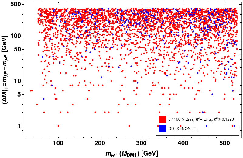
(a)

(b)

Figure 7: Relic and direct search outcome for (a) scalar DM and (b) fermion DM. The red points satisfy relic density requirement and the blue points satisfy direct detection bound (XENON 1T) as well as relic density constraints.

Figure 8: Regions allowed by indirect detection constraints from $W^{+}W^{-}$ mode for scalar and fermionic DM. Their individual contributions have been scaled by their respective number density.

In Fig. 8, we show the regions allowed by indirect detection constraints. Due to gauge interaction, the major annihilation channels for both SDM and FDM occurs into $W^{+}W^{-}$ final state. Therefore, the most stringent upper limit comes from this particular channel in MAGIC MAGIC:2016xys plus Fermi-LAT data Fermi-LAT:2015att . Similar to direct search, while calculating the annihilation cross-section of each DM into $W^{+}W^{-}$ final state, we have scaled their individual contribution consistently with the corresponding DM densities to the total relic density. One can see that the entire range of DM parameters scanned here satisfy the upper limit from indirect searches.

4 Selection of benchmark points

Having discussed all the constraints on the model and carefully examining various possibilities for distinguishing two peaks in kinematic distributions for two-component DM, we are in a position to choose a few benchmark points, suited for the likely centre-of-mass energies of $e^{+}e^{-}$ colliders planned for the near future, including the International Linear Collider (ILC). Relevant kinematic regions (allusions to some have already been discussed) where the peaks can be distinguished are as follows:

• Region I:  $m_{\rm DM_{1}}>m_{\rm DM_{2}}$ and $\Delta m_{1}>\Delta m_{2}$ ,

• Region II:  $m_{\rm DM_{1}}<m_{\rm DM_{2}}$ and $\Delta m_{1}<\Delta m_{2}$ ,

• Region III:  $m_{\rm DM_{1}}<m_{\rm DM_{2}}$ and $\Delta m_{1}>\Delta m_{2}$ ,

• Region IV:   $m_{\rm DM_{1}}>m_{\rm DM_{2}}$ and $\Delta m_{1}<\Delta m_{2}$ .

Recall that subscript 1 above refers to SDM sector and 2 to FDM sector. However, distinguishability of the peaks at collider crucially depend on the relative cross-sections ($\sigma$) of the two dark sector particles, which makes some of these kinematic regions more favourable than the others. We therefore make a quantitative comparison between the scalar and fermionic HDSP pair production cross-sections in Fig. 9, where (a) $\sigma_{\phi^{+}\phi^{-}}$ and (b) $\sigma_{\psi^{+}\psi^{-}}$ are plotted as a function of $\sqrt{s}$ for different choices of HDSP masses using unpolarised initial beams . In Fig. 9, the range of $\sqrt{s}$ is varied between 500 GeV to 1 TeV as per the technical design report of ILC Adolphsen:2013kya ; Bambade:2019fyw ; Zarnecki:2020ics .

We recall here that $\psi^{+}$ and $\psi^{-}$ have vector-like couplings to both $\gamma$ and $Z$ as follows,

$$\psi^{+}\psi^{-}Z:-~{}ie_{0}\cot(2\theta_{W})\gamma^{\mu}~{},$$ (23)

$$\psi^{+}\psi^{-}\gamma:-~{}ie_{0}\gamma^{\mu}\,.$$ (24)

The charged scalar couplings with $\gamma$ and $Z$ are momentum-dependent and are given by,

$$\phi^{+}\phi^{-}Z:-~{}ie_{0}\cot(2\theta_{W})(p_{1}^{\mu}-p_{2}^{\mu})~{},$$ (25)

$$\phi^{+}\phi^{-}\gamma:-~{}ie_{0}(p_{1}^{\mu}-p_{2}^{\mu})\,,$$ (26)

where $p_{1}^{\mu}$ and $p_{2}^{\mu}$ are the four-momenta of the outgoing charged scalars.

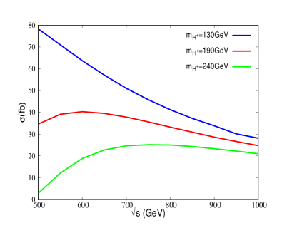
(a)

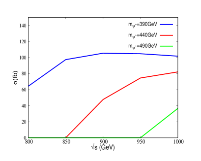
(b)

Figure 9: Production cross-section of HDSP pair for (a) scalar $\phi^{+}\phi^{-}$ and (b) fermion $\psi^{+}\psi^{-}$ as a function of $\sqrt{s}$ for different choices of HDSP masses at ILC. We use unpolarized initial beams. All the relevant couplings for the production of HDSP’s are given in Eqs. 23-26.

Scalar HDSP has smaller production cross-section compared to the fermionic ones for the same mass, because of the absence of polarization sum in the former, as is also clear from Fig. 9. We would then ideally use for illustration, a lighter $\phi^{\pm}$ and heavier $\psi^{\pm}$ in order for them to have comparable production rates. From this viewpoint, Region I proves to be underwhelming while Region II appears favourable. However, with large mass splitting in the FDM sector ($\Delta m_{1}<\Delta m_{2}$ as in Region II), we need to restrict to the Higgs resonance region with $m_{\psi_{1}}\approx\frac{m_{h}}{2}\sim 60$ GeV (see Fig. 7(b)) to address DM constraints. Therefore, in Region II, one requires even lighter scalar DM with relatively large $\Delta m_{1}$, so that cross-sections for SDM is comparable to that of FDM. This leads to a broad peak in $\not{E}$ from the scalar sector which eventually merges partially with the peak coming from the fermion sector.

We will actually have large accessible regions consistent with $m_{\rm DM_{1}}>m_{\rm DM_{2}}$ in Region IV. As small $\Delta m$ would imply a narrow $\not{E}$ distribution, $\Delta m_{1}<\Delta m_{2}$ provides a narrow distribution in the scalar dark sector (with smaller cross-section), and a wider one for fermions (with larger cross-section), a much needed feature for the separation of two peaks. In Region III with $m_{\rm DM_{1}}<m_{\rm DM_{2}}$, and $\Delta m_{1}>\Delta m_{2}$, the FDM is almost degenerate with HDSP to address DM constraints, while the SDM has a larger mass gap from the corresponding HDSP, which is possible only with $m_{\phi^{0}}\sim\frac{m_{h}}{2}$ to account for DM constraints. In this case, we will then end up with a narrow distribution in the FDM sector, and a wider one for the SDM sector. The relative cross-section of the scalar and fermion DM production makes this scenario hard to distinguish. Therefore, Region IV turns most favourable in the context of the model at hand for probing two-component DM signature at ILC with reasonable $\sqrt{s}$. The discussion above also elucidates how DM constraints together with production cross-section can favor a specific region over the others.

In Table 2, we identify four benchmark points from Region IV, out of which BP1 and BP2 can be probed with $\sqrt{s}=$ 1 TeV, while BP3 and BP4 can be probed with $\sqrt{s}=500$ GeV. The scalar sector is kept fixed at $m_{\rm DM_{1}}=100$ GeV, $\Delta m_{1}=10$ GeV and $\lambda_{L}=0.01$. As argued before, FDM is chosen around the Higgs resonance for cosmological constraints, so that the essential difference amongst the benchmark points lies in the values of $\Delta m_{2}$ and $\sin\theta$ in FDM sector. We also present the individual DM relic densities and spin-independent direct detection cross-section for all the benchmarks together with invisible branching ratio of Higgs for each cases to show that they satisfy all the limits. The relic density for SDM is minuscule $\Omega_{\phi^{0}}h^{2}\approx 0.0022$, while the effective spin independent direct search cross-section (following Eq. 21) $\sigma_{\phi^{0}}^{\rm eff}\approx 10^{-46}$ cm² is well within the limit. FDM shares the major relic density with $\Omega_{\psi_{1}}h^{2}\approx 0.11$ with $\sigma_{\psi_{1}}^{\rm eff}\approx 10^{-47}$ cm². The relative contribution of SDM to observed relic can be increased via increasing SDM mass. However, that will come at a cost of reduced production cross-section of SDM and consequently, poor distinguishability of the two peaks.

BPs	SDM sector $\{m_{\phi^{0}},~{}\Delta m_{1},~{}\lambda_{L}\}$	FDM sector $\{m_{\psi_{1}},~{}\Delta m_{2},\sin\theta\}$	$\Omega_{\phi^{0}}h^{2}$	$\Omega_{\psi_{1}}h^{2}$	$\sigma_{\phi^{0}}^{\rm eff}$ (cm2)	$\sigma_{\psi_{1}}^{\rm eff}$ (cm2)	BR($H_{\rm inv}$)$\%$
BP1	$100,~{}10,~{}0.01$	$60.5,~{}370,~{}0.022$	$0.00221$	$0.1195$	$3.45\times 10^{-46}$	$2.03\times 10^{-47}$	$0.25$
BP2	$100,~{}10,~{}0.01$	$58.91,~{}285,~{}0.032$	$0.00221$	$0.10962$	$3.45\times 10^{-46}$	$5.38\times 10^{-47}$	$1.60$
BP3	$100,~{}10,~{}0.01$	$58.87,~{}176,~{}0.04$	$0.00221$	$0.11941$	$3.45\times 10^{-46}$	$5.00\times 10^{-47}$	$1.50$
BP4	$100,~{}10,~{}0.01$	$58.48,~{}190,~{}0.042$	$0.00221$	$0.1114$	$3.45\times 10^{-46}$	$7.01\times 10^{-47}$	$2.4$

Table 2: Benchmark points of the model; contribution to relic density, spin-independent direct detection cross-section as well as that of invisible Higgs decay branching ratios of the DM components $\phi^{0}$ and $\psi_{1}$ are mentioned.

5 Signal and background

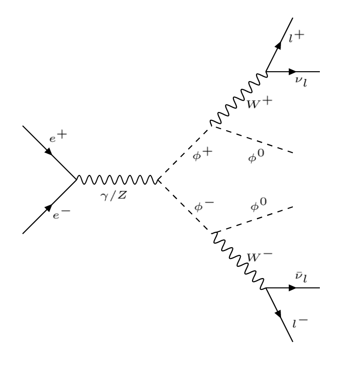
(a)

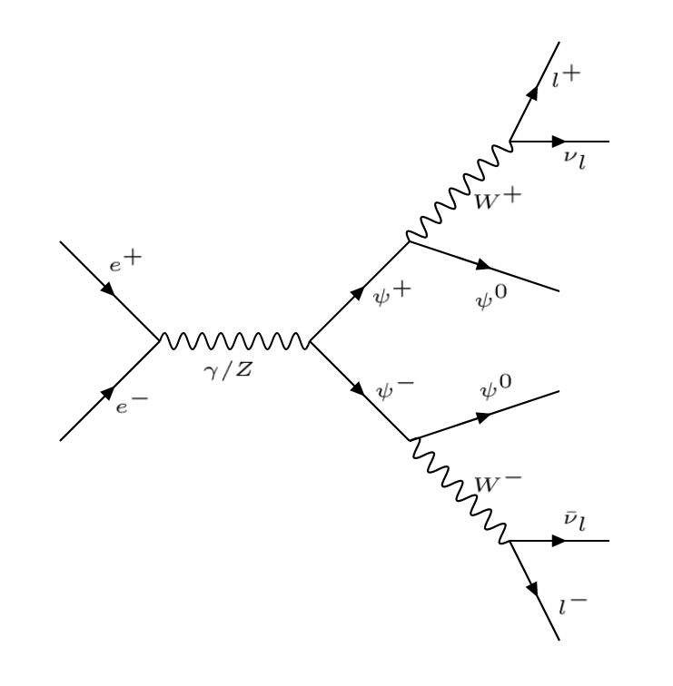
(b)

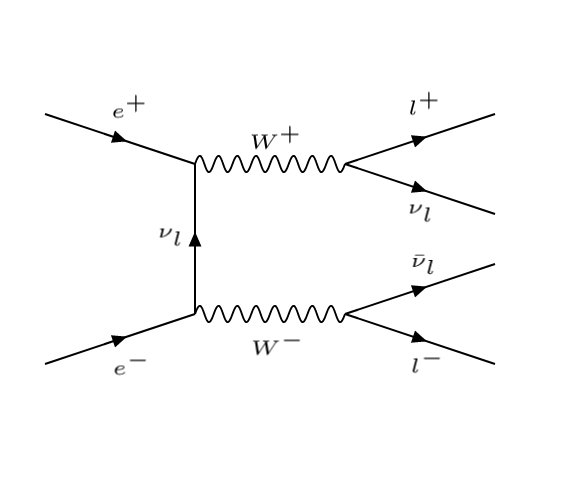
(c)

(d)

Figure 10: Dominant process contributing to $\ell^{+}\ell^{-}+\not{E}$ at ILC from the two component dark sector signal (top) and $WW$ and $ZZ$ background (bottom).

The final state of our interest is $\ell^{+}\ell^{-}+\not{E}$. We demand two isolated opposite-sign dileptons (OSD) with both $e,\mu$ and $p_{T}>10$ GeV for each of them. The isolation criterion for the leptons demands ${\frac{|p^{\ell}_{T}|}{\Sigma^{i}|p^{i}_{T}|}}<0.12$, where the summation in the denominator is over all the particles within $\Delta R=0.5$ around each lepton. Events for the signal and backgrounds have been generated using Madgraph@MCNLO Alwall:2014hca . The detector simulation has been taken care of by Delphes-3.4.1 deFavereau:2013fsa with ILD specifications.

The following HDSP production and subsequent decay chains involving NP as per the model contribute dominantly to this final state.

$e^{+}e^{-}\rightarrow\phi^{+}\phi^{-},\phi^{+}\rightarrow W^{+(*)}\phi^{0},W^{+(*)}\rightarrow\ell^{+}\nu_{\ell},\phi^{-}\rightarrow W^{-(*)}\phi^{0},W^{-(*)}\rightarrow\ell^{-}\bar{\nu}_{\ell}$

$e^{+}e^{-}\rightarrow\psi^{+}\psi^{-},\psi^{+}\rightarrow W^{+(*)}\psi_{1},W^{+(*)}\rightarrow\ell^{+}\nu_{\ell},\psi^{-}\rightarrow W^{-(*)}\psi_{1},W^{-(*)}\rightarrow\ell^{-}\bar{\nu}_{\ell}$

The SM background processes that will lead to same final state are as follows:

$e^{+}e^{-}\rightarrow W^{+}W^{-},W^{+}\rightarrow\ell^{+}\ell_{\nu},W^{-}\rightarrow\ell^{-}\bar{\nu_{\ell}}$

$e^{+}e^{-}\rightarrow W^{+}W^{-}Z,W^{+}\rightarrow\ell^{+}{\nu_{\ell}},W^{-}\rightarrow\ell^{-}\bar{\nu_{\ell}},Z\rightarrow\nu_{\ell}\bar{\nu}_{\ell}$

$e^{+}e^{-}\rightarrow ZZ,Z\rightarrow\ell^{+}\ell^{-},Z\rightarrow\nu_{\ell}\bar{\nu}_{\ell}$

In Fig. 10, we show all the major Feynman diagrams contributing to the final state $\ell^{+}\ell^{-}+\not{E}$ from the DM signal and the dominant SM background processes. Out of the SM contributions, $e^{+}e^{-}\rightarrow W^{+}W^{-}$ has the largest production cross-section. The most efficient way to reduce this background is the use of beam polarization, which we discuss next. $e^{+}e^{-}\rightarrow ZZ$ constitutes another copious background, while $e^{+}e^{-}\rightarrow W^{+}W^{-}Z$ has much lesser production cross-section. It should be noted that a large background contribution comes from non-resonant production of $e^{+}e^{-}\rightarrow\nu\bar{\nu}Z$, where the $\nu\bar{\nu}$ pair is not coming from $Z$. This process primarily involves $t$-channel $W$ mediated diagrams. The cross-section at $\sqrt{s}=1$ TeV is 50% of $WW$ background and at $\sqrt{s}=500$ GeV is of similar magnitude to that of $ZZ$ production. However, a strong cut on the invariant mass of the lepton pair, (demanding it to be outside $Z$ mass window) will considerably reduce this background.

5.1 Effect of beam polarization

$e^{+}e^{-}\rightarrow W^{+}W^{-}$ receives dominant contribution via $t$-channel neutrino exchange (see Fig. 10), involving left-handed electrons and right-handed positrons. This process can thus be suppressed with maximally right polarized $e^{-}$ beam and maximally left polarised $e^{+}$ beam. At ILC, the electron polarization is proposed to be maximum 80% whereas, the positron polarization is expected to be 30% with a possible upgradation to 60% Behnke:2013lya . In Fig. 11, we compare $\not{E}$ distributions for BP1 (at $\sqrt{s}=$ 1TeV) with dominant SM backgrounds for various degrees of beam polarization, defined by P1 $\equiv$ $\{P_{e^{-}}:-0.8,P_{e^{+}}:+0.3\}$, P2 $\equiv\{P_{e^{-}}:0,P_{e^{+}}:0\}$ and P3 $\equiv\{P_{e^{-}}:+0.8,P_{e^{+}}:-0.3\}$, where $+(-)$ denotes right(left) polarisation. We clearly see the effect of polarization in reducing the dominant $WW$ background. One can see that the initial beam polarization affects the signal cross-section too. However, the effect is much milder compared to the background. A similar observation can be made for BP3 at $\sqrt{s}=$ 500 GeV. We note further that the sub-dominant $e^{+}e^{-}\rightarrow ZZ$, gets major contribution from lepton mediated $t$-channel diagrams (see Fig. 10), thus receives little suppression from the beam polarization of the above type. The non-resonant $\nu\bar{\nu}Z$ background, on the other hand, receives substantial suppression from the particular beam polarization configuration that we consider. The cross-sections for DM signal at the benchmark points are mentioned in Table 3, while those from SM background is mentioned in Table 4. It is evident that $S/B$, where $S$ refers to signal and $B$ refers to background events, will be the largest for polarization configuration P3. We further see that $WWZ$ background plays negligible role in the analysis, due to its dismal cross-section. Therefore, we omit the distributions for $WWZ$ background in all the forthcoming discussions.

Benchmarks		Collider cross-section (fb)
		$\sigma_{\rm total}$(OSD)			$\sigma_{\phi^{+}\phi^{-}}$(OSD)			$\sigma_{\psi^{+}\psi^{-}}$(OSD)
$\sqrt{s}$	Points	P1	P2	P3	P1	P2	P3	P1	P2	P3
1000	BP1	232(10.8)	115(5.5)	58.5(2.75)	57.4(2.9)	28.9(1.5)	14.5(0.75)	173(8.4)	83.0(4.0)	44.0(2.0)
	BP2	276(13.4)	141(6.6)	70.0(3.3)	57.4(2.9)	28.9(1.5)	14.5(0.75)	218(10.4)	111(5.3)	55.5(2.7)
500	BP3	686(33.0)	339(15.9)	168.1(7.8)	180(8.9)	90.3(4.5)	44.3(2.3)	494(22.2)	253(11.3)	123.8(5.5)
	BP4	345(16.7)	170(8.4)	83.5(3.9)	180(8.9)	90.3(4.5)	44.3(2.3)	171.4(7.4)	82.4(3.9)	39.2(1.9)

Table 3: Signal cross-sections for HDSP pair production (OSD final state) at ILC. Total cross-section ($\sigma_{\rm tolal}$), as well as individual contributions from SDM ($\sigma_{\phi^{+}\phi^{-}}$) and FDM ($\sigma_{\psi^{+}\psi^{-}}$) are mentioned. Three choices of beam polarisation are used: P1 $\equiv$ $\{P_{e^{-}}:-0.8,P_{e^{+}}:+0.3\}$, P2 $\equiv\{P_{e^{-}}:0,P_{e^{+}}:0\}$ and P3 $\equiv\{P_{e^{-}}:+0.8,P_{e^{+}}:-0.3\}$. CM energy ($\sqrt{s}$) is in the units of GeV.

Backgrounds		Cross-section(fb)
$\sqrt{s}$	Processes	P1	P2	P3
1 TeV	$WW$	296	128	18.3
	$ZZ$	7.5	4.4	3.5
	$WWZ$	1.2	0.5	0.08
500 GeV	$WW$	802	342	51
	$ZZ$	21	12	9.6
	$WWZ$	0.8	0.37	0.06

Table 4: Production cross-sections for $W^{+}(\ell^{+}\nu)W^{-}(\ell^{-}\bar{\nu})$, $Z(\ell^{+}\ell^{-})Z(\nu\bar{\nu})$ and $W^{+}(\ell^{+}\nu)W^{-}(\ell^{-}\bar{\nu})Z(\nu\bar{\nu})$ background at $\sqrt{s}$ = 1 TeV and 500 GeV for various polarization combinations P1, P2 and P3 (see caption of Table 3).

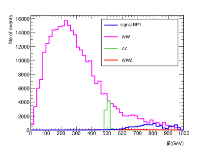
(a)

(b)

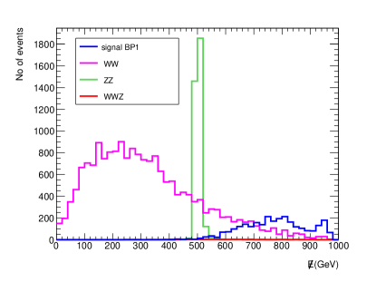
(c)

Figure 11: Unnormalized $\ell^{+}\ell^{-}$ event distribution for $\not{E}$ at ILC with $\sqrt{s}$ = 1 TeV and $\mathcal{L}=$ 1000 ${\rm fb}^{-1}$ for BP1 along with $WW$ and $ZZ$ backgrounds for various degrees of beam polarisation, (a) P1, (b) P2 and (c) P3 (see caption of Table  3 and text).

6 Analysis with selected benchmark points

6.1 Analysis at $\sqrt{s}=$ 1 TeV

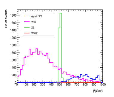
(a)

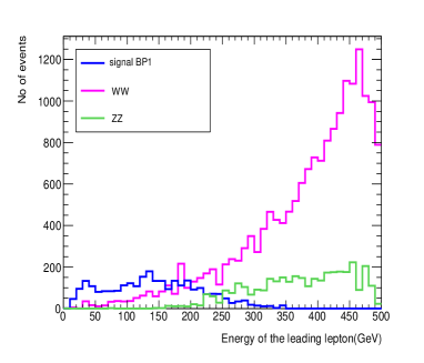
(b)

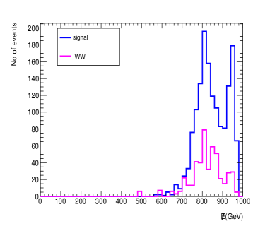
(c)

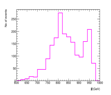
(d)

Figure 12: Unnormalized distribution of (a) missing energy, (b) energy of the leading lepton, (c) missing energy after applying the cut on the energy of leading lepton $<$ 150 GeV for DM signal and SM backgrounds, (d) missing energy distribution of signal from BP1 plus background after applying the cut $E_{\ell_{1}}<150$ GeV at ILC with $\sqrt{s}=$ 1 TeV, beam polarisation P3 (see text) at $\mathcal{L}=$1000 ${\rm fb}^{-1}$.

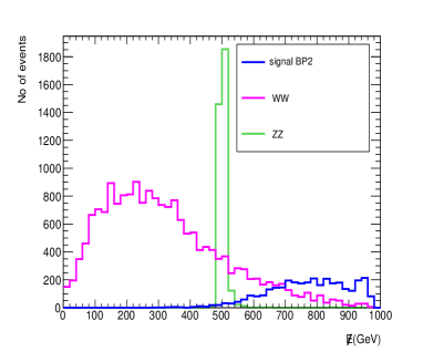
(a)

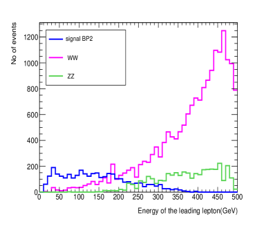
(b)

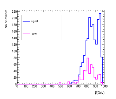
(c)

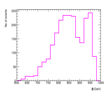
(d)

Figure 13: Same as Fig. 12 but for BP2.

We take up first BP1 and BP2, which, due to their higher masses, can only be probed at $\sqrt{s}=1$ TeV. In Fig. 12 (a), we show the corresponding $\not{E}$ distribution for signal (BP1) and dominant backgrounds at $\mathcal{L}=$1000 ${\rm fb}^{-1}$ of integrated luminosity with beam polarisation P3 $\equiv\{P_{e^{-}}:0.8,P_{e^{+}}:-0.3\}$. As one can clearly see, the $\not{E}$ distribution for the signal peaks at a higher value compared to that for the SM backgrounds. It is observed that, in case of $W^{+}W^{-}$ background, the leptons carry most of the energy and therefore, the $\not{E}$ peaks at a lower value. In case of $ZZ$ background, the energy is shared comparably between the two $Z$ bosons. Therefore $\not{E}$ peaks at $\frac{\sqrt{s}}{2}$ i.e. at 500 GeV. The signal distribution on the other hand, has two peaks. The peak at lower $\not{E}$ corresponds to FDM and the higher one arises from SDM, as $m_{\psi_{1}}<m_{\phi_{0}}$. The scalar sector being almost degenerate shows much narrower peak compared to the fermionic case, where $\Delta m_{2}$ is comparatively large and the distribution is flatter. In Fig. 12 (b), we plot the energy of the leading lepton. As the total energy of collision is fixed at ILC, the energy distribution of the leading lepton shows a sharp complementarity with the $\not{E}$. It peaks at a higher value for the backgrounds and at a lower value for signal. Lepton energy distribution also retains the double-peak behaviour like $\not{E}$ distribution. Next we apply a cut on the energy of the leading lepton and as a result, $\not{E}$ distribution of the $W^{+}W^{-}$ background becomes significantly softer (see Fig. 12(c)). The resulting position and size of the peak of the $W^{+}W^{-}$ background distribution is pretty sensitive to the lepton energy cut applied. For example, in this case when we apply $E_{\ell_{1}}<150$ GeV, the peak from $W^{+}W^{-}$ distribution coincides with the first peak of the signal, and the distinction between the resulting first and second peak become even more prominent. The extent at which the value of this cut affects our analysis will be discussed shortly. It may be noted that the contribution from $ZZ$ background becomes negligible after applying the leading lepton energy cut and therefore is not shown explicitly in Fig. 12(c). We further show in Fig. 12(d) the final signal plus background distribution after applying the aforementioned cut. We can see that the two peaks can be distinguished rather well, even in the presence of background events.

We perform the same analysis for BP2 and resulting distributions are shown in Fig. 13. The separation between two signal peaks is slightly worse here pertaining to smaller $\Delta m_{2}$ compared to BP1. However, after applying the leading lepton energy cut, the first peak, as well as $WW$ background gets diminished and the heights of the two peaks in the signal plus background $\not{E}$ distribution become comparable. We further note here that, in this case after applying the cut $E_{\ell_{1}}<150$ GeV, the background distribution does not exactly coincide with the first peak of the signal (Fig. 13(c)) and therefore, the first peak of the signal plus background distribution (Fig. 13(d)) is flatter compared to BP1 as in Fig. 12.

6.2 Analysis at $\sqrt{s}=$ 500 GeV

For BP3 and BP4, it is possible to produce HDSPs on-shell at $\sqrt{s}=500$ GeV. It is evident that with smaller charged fermion mass, the size of the first peak in $\not{E}$ distribution is bigger in both cases compared to the second. This reduces the visibility of the double hump behaviour. The lepton energy cut is modified to $E_{\ell_{1}}<75$ GeV for both these cases, which reduces the area under first peak. Remaining $WW$ background events adds to the first peak, resulting a double peak in $\not{E}$ distribution for both the benchmark points. The case for BP4 is only shown in Fig. 14; the organisation remains same as in Fig. 12. The limitations of kinematical regions like Region III to see a distinguishable double peak in presence of SM background is discussed in Appendix C.

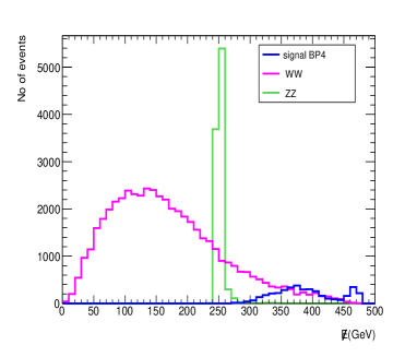
(a)

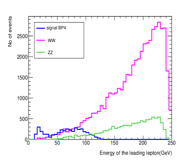
(b)

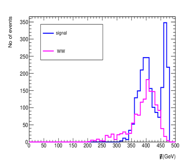
(c)

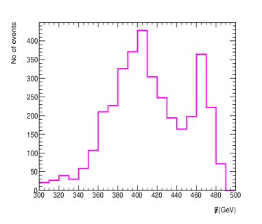
(d)

Figure 14: Same as Fig. 12, but for BP4 at $\sqrt{s}=$ 500 GeV with $E_{\ell_{1}}<$ 75 GeV.

6.3 Impact of lepton energy cuts

As pointed out earlier, at the $e^{+}e^{-}$ collider, the lepton energy distribution shows a complementarity with $\not{E}$ distribution. A cut on the energy of the leading lepton suppresses the background and also helps us retain the Gaussian nature of the resulting distribution. However, the choice of the cut is crucial. As the total energy of collision in each event is fixed, higher lepton energy naturally corresponds to smaller $\not{E}$. Therefore, an upper cut on the lepton energy immediately indicates a lower cut-off in $\not{E}$ distribution. Given that $\not{E}$ distribution peaks at a much lower value for $WW$ compared to the DM signal, an upper cut on lepton energy distribution eliminates the low $\not{E}$ region. Harder lepton energy cut pushes the $\not{E}$ distribution from $WW$ events towards larger $\not{E}$. Naturally, the first peak on lower $\not{E}$ from the signal is also affected by this cut. But, the second peak remains unaffected as long as the lepton energy cut is not too hard. Therefore optimising lepton energy cut so that $WW$ distribution coincides with the first peak of the signal elucidates the double hump behaviour. This is shown in Fig. 15, where we compare $\not{E}$ distribution after applying (a) $E_{\ell_{1}}<$ 150 GeV and (b) $E_{\ell_{1}}<$ 200 GeV.

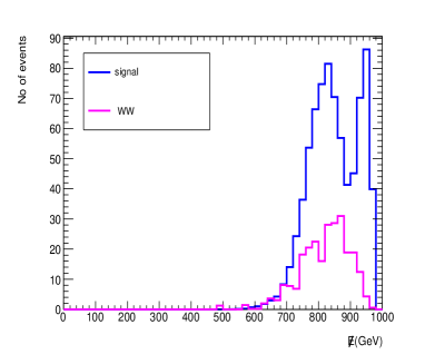
(a)

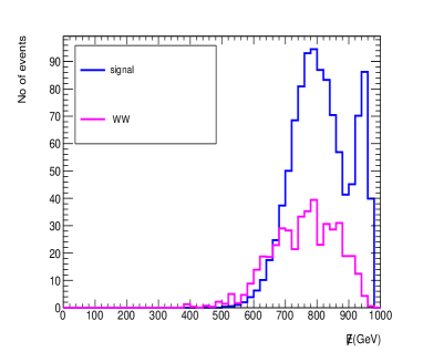
(b)

Figure 15: Signal (BP1) and SM background distribution after applying cuts (a) $E_{\ell_{1}}<150$ GeV and (b) $E_{\ell_{1}}<200$ GeV with $\sqrt{s}=$ 1 TeV for polarisation P3 (see text) at ILC.

6.4 Signal significance

Before going into the quantitative discussion on distinguishability of the two DM peaks, we briefly examine the discovery potential of $\ell^{+}\ell^{-}+\not{E}$ signal at ILC by calculating signal significance (${\cal S}$) defined as follows:

$${\cal S}=\sqrt{2[(S+B)\text{Log}(1+\frac{S}{B})-S]}\,;$$ (27)

where $S$ and $B$ are the signal and background events surviving after all the analysis cuts are applied. We use the following selection cuts, apart from the basic ones:

• $\sqrt{s}=1$ TeV: (i) Cut on the energy of the leading lepton $E_{\ell_{1}}<150$ GeV, (ii) $\not{E}>600$ GeV, (iii) Invariant mass cut on the lepton pair, $60<m_{\ell\ell}<120$ GeV.

• $\sqrt{s}=500$ GeV: (i) Cut on the energy of the leading lepton $E_{\ell_{1}}<75$ GeV, (ii) $\not{E}>300$ GeV, (iii) Invariant mass cut on the lepton pair, $70<m_{\ell\ell}<110$ GeV.

We remind the reader that the strong invariant mass cut of the lepton pair has been applied in order to reduce the non-resonant $\nu\bar{\nu}Z$ background, as discussed earlier. We present ${\cal S}$ for all the benchmarks for various polarization combinations of initial beams in Table 5 for $\mathcal{L}$=100 ${\rm fb}^{-1}$. We note here that for the particular polarization combination P1, one can achieve the maximum ${\cal S}$. However, with P2 and P3 too, it is possible to achieve ${\cal S}\raisebox{-3.69899pt}{~{}\shortstack{$>$ \\ [-0.07cm] $\sim$}}~{}8\sigma$ for all the benchmark points. Therefore, all the aforementioned polarization combinations can ensure a significant discovery potential of our purported signal.

In addition to ${\cal S}$, we present $S/B$ in Table 5, which gives us an estimate of the amount of signal purity or background contamination in the final kinematical distribution. To ensure that the two-peak signature is actually coming from the signal pertaining to two different DM particles, one should demand a large $S/B$. We see that $S/B$ maximizes for the polarization combination P3, which justifies our choice of polarization of initial beams as chosen in the rest of the analysis. We would like to point out that along with ${\cal S}$ and $S/B$, the distinguishability of two peaks also depend on the absolute number of observed events, which is proportional to the integrated luminosity $\int Ldt$. We use abbreviation $\int Ldt\equiv\mathcal{L}$ to denote the same in the rest of the analysis and discuss the effect of $\mathcal{L}$ on the distinguishability of the two peaks in the next section.

Benchmarks	$S/B$			${\cal S}$
	P1	P2	P3	P1	P2	P3
BP1	1.07	0.91	3.7	14.5	9.7	11.3
BP2	1.2	1.05	4.2	16.2	11.0	12.4
BP3	1.05	1.13	3.4	22.0	16.1	17.4
BP4	0.4	0.5	1.5	10.7	8.0	8.5

Table 5: $S/B$ and signal significance (${\cal S}$) for different benchmark points for various beam polarizations, P1, P2, P3 (see text). ${\cal S}$ has been calculated for $\mathcal{L}$ = 100 ${\rm fb}^{-1}$.

7 Distinction criteria for two peaks in $\not{E}$ spectrum

As demonstrated above, two different dark sectors having DM masses $m_{\rm DM_{1}}$, $m_{\rm DM_{2}}$, and mass differences $\Delta m_{1}$ and $\Delta m_{2}$ with the HDSP, yielding same collider signal, will provide peaks at different values in $\not{E}$ distribution. These peaks partially overlap when the full signal produced from both dark sector is analysed. It is also shown that when the difference between masses and/or splitting becomes large, the two peaks in distorted $\not{E}$ distribution is more prominent. Such $\not{E}$ distributions of the signal with reduced SM background can therefore be fitted into a two-peak asymmetric Gaussian distribution as a function of any variable $x$ as:

$$G(x) = G_{1}(x)+G_{2}(x)+\cal{B}$$ (28)

$$= A_{1}~{}e^{-\frac{(x-\mu_{1})^{2}}{2\sigma_{1}^{2}}}+A_{2}~{}e^{-\frac{(x-\mu_{2})^{2}}{2\sigma_{2}^{2}}}+\cal{B}~{}.$$

Here $G_{1}(x)$ is the Gaussian function corresponding to the first peak with amplitude $A_{1}$, mean $\mu_{1}$, and standard deviation $\sigma_{1}$; while $G_{2}(x)$ is the function containing the corresponding quantities for the second DM peak. The constant (or slowly varying) parameter $\cal{B}$ is further introduced to account for various theoretical uncertainties as well as those due to $\not{E}$ mis-measurement etc. A schematic of such a function is shown in Fig. 16. Here onwards we also introduce a simplified notation to denote $\not{E}$ by $t$ and $\frac{d\sigma}{d\not{E}}$ by $y$.

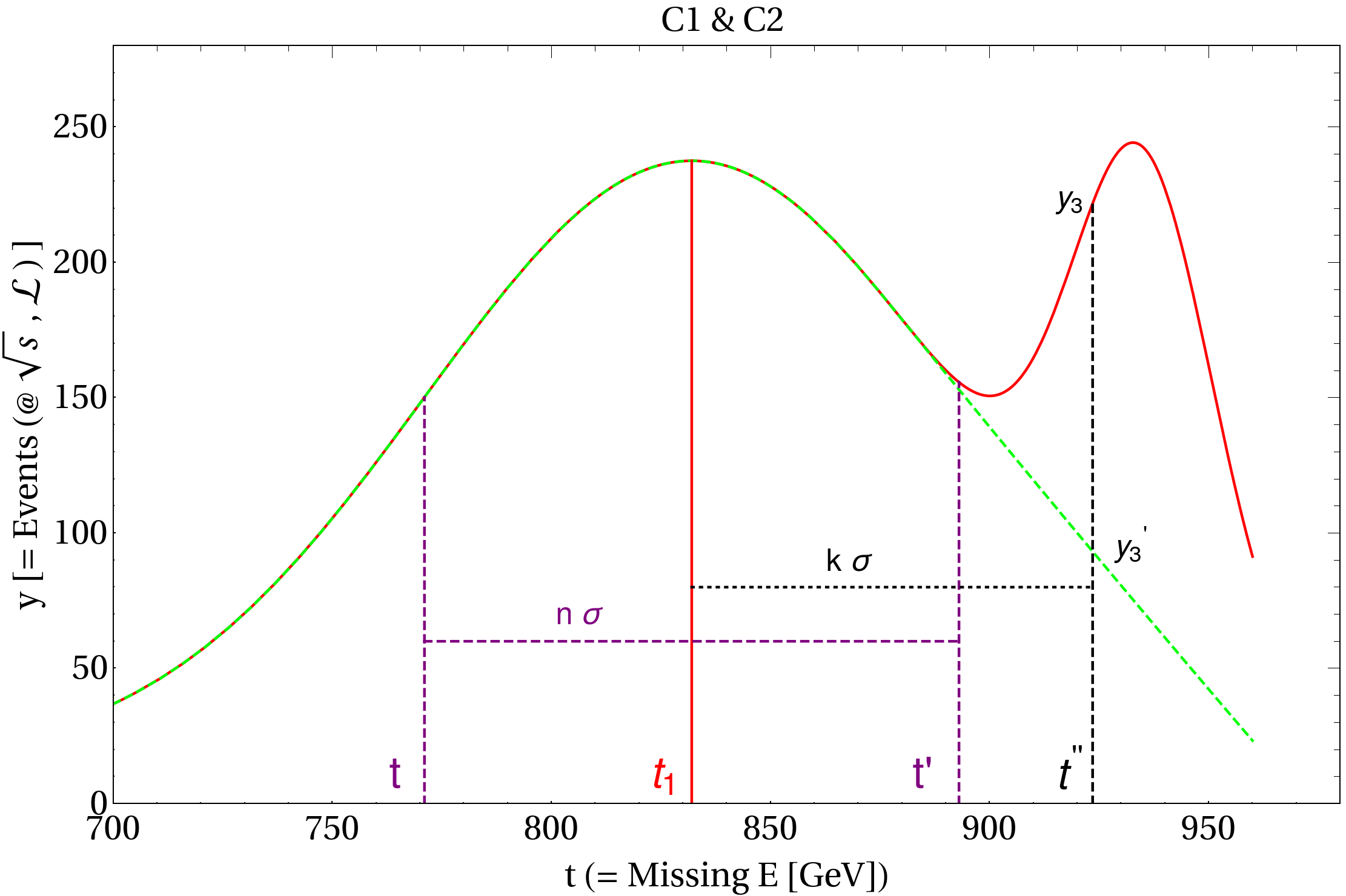
(a)

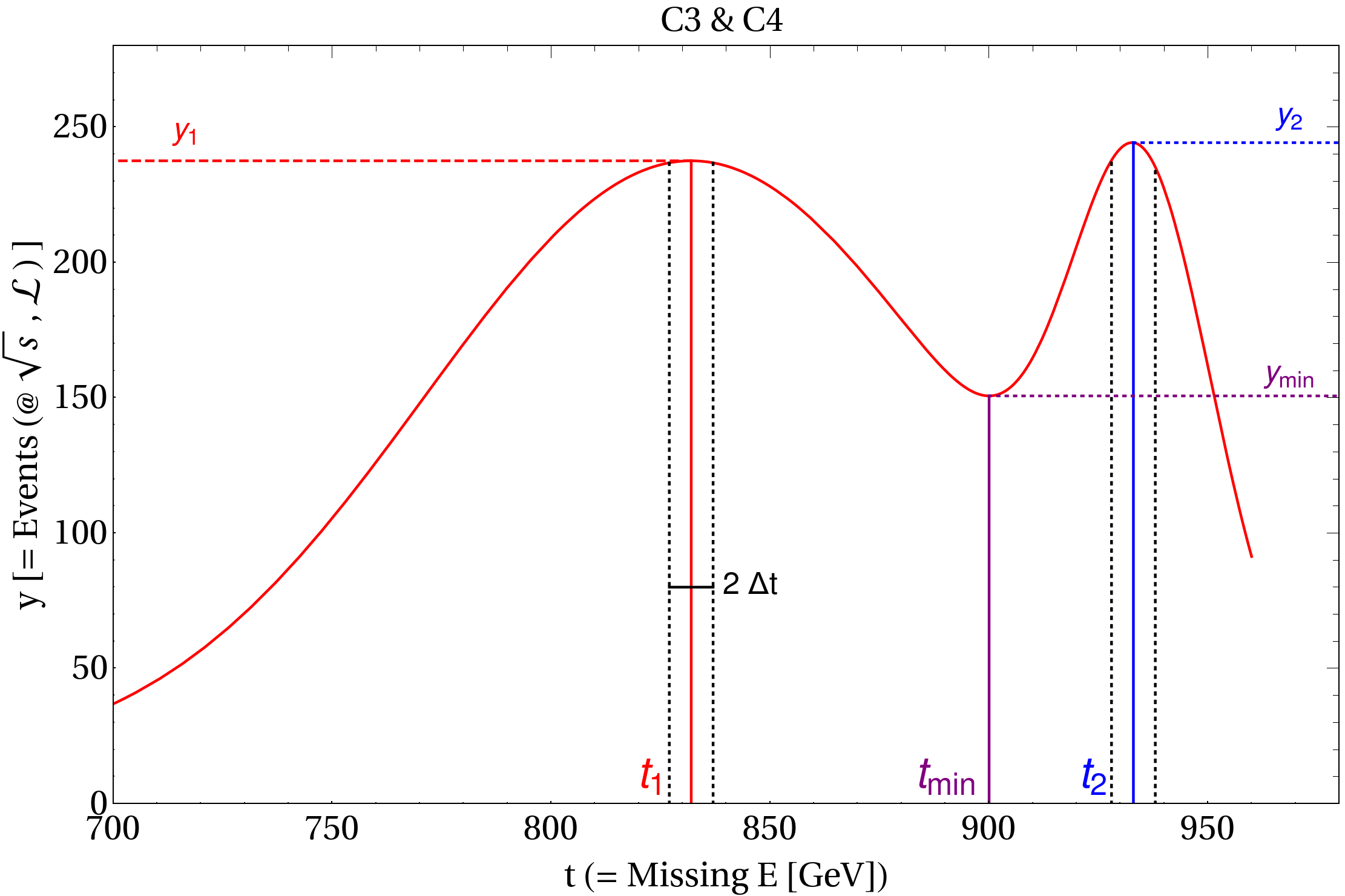
(b)

Figure 16: A schematic representation of a typical $\not{E}$ distribution in $\frac{d\sigma}{d\not{E}}(\equiv y)~{}\rm{vs}~{}\not{E}(\equiv t)$ plane with two peaks when fitted with Gaussian function as in Eq. 28 is shown. Left: quantities required for conditions C1 and C2 are defined (see text for details); Right: quantities required for conditions C3 and C4 are defined.

Let us now assume that we can identify two peaks at $\not{E}$ values $t_{1}(\equiv\mu_{1})$ and $t_{2}(\equiv\mu_{2})$ as shown in Fig. 16. The number of events at those peaks are denoted by $y_{1}=y(t_{1})$ and $y_{2}=y(t_{2})$ respectively; which are nothing but the area under the curve in a small interval around the peak as indicated in the right hand side figure. The minima between two peaks is identified as $t_{\rm min}$ and the corresponding event rate along y-axis is denoted by $y_{\rm min}$. With this preliminaries, we are now ready to set up the criteria for distinguishing the two peaks in $\not{E}$ spectra. Each such criterion must address either or both of the following questions: (a) How to elicit the prominence of the second (read smaller) peak relative to the first (bigger) peak, and (b) How to resolve best the separation between the two peaks.

• C1: The first condition examines how much the presence of second peak distorts the symmetry of the distribution about the first peak. This will require us to compare the number of events within n$\sigma$ ($n\geq 1$) range of the first peak on both sides. Let us assume, $t$ (on left) and $t^{\prime}$ (on right) are the two positions which are n$\sigma$ ($n\geq 1$) away from the first peak $t_{1}$ as shown in Fig. 16(a). Assume number of events within n$\sigma$ on both sides of the first peak as:

  $$\Delta N_{1}=\int_{t}^{t_{1}}ydt,~{}~{}\Delta N_{2}=\int_{t_{1}}^{t^{{}^{\prime}}}ydt\,.$$ (29)

  We define

  $$R_{C1}=\frac{|\Delta N_{2}-\Delta N_{1}|}{\sqrt{\Delta N_{1}}}\,.$$ (30)

  Then if

  $$R_{C1}>2\,,$$ (31)

  we can stipulate that the peaks are resolved to 2$\sigma$ significance or larger. Note that the denominator in Equation (31) represents the fluctuation of the distribution corresponding to the first peak. The criterion C1, defined in terms of integrated quantities, is useful when the two peaks are not visually prominent but a distortion to the $\not{E}$ spectrum occurs. It is also worth registering that this criterion has its limitation when the second peak is much smaller than the first.

• C2: The second condition addresses how high does the second peak go. Let us assume $y_{3}=y(t^{{}^{\prime\prime}})$ is the number of events at $t^{{}^{\prime\prime}}$ which is assumed to be $k\sigma$ ($k\geq 1$) away from the first peak $t_{1}$ on the right side and $y_{3}^{\prime}=y^{\prime}(t^{{}^{\prime\prime}})$ is the corresponding number of events in the absence of second peak upon a Gaussian fit (Fig. 16(a)). Then we define $R_{C2}$ in terms of the difference between these two numbers as follows:

  $$R_{C2}=\frac{y(t^{{}^{\prime\prime}})-y^{\prime}(t^{{}^{\prime\prime}})}{\sqrt{y^{\prime}(t^{{}^{\prime\prime}})}}\equiv\frac{y_{3}-y_{3}^{{}^{\prime}}}{\sqrt{y_{3}^{{}^{\prime}}}}\,.$$ (32)

  If $R_{C2}>2$, we will be able to say that the fluctuation is more than 2$\sigma$ and can be termed as a second peak. Note that C2 offers a criterion at the differential level, in contrast with C1, which comes at an integral level.

• C3: Another possibility to check how significant the second peak is to compare the number of events within a close window ($\Delta t\sim$ 5 GeV) around two peaks as shown in Fig. 16(b). One may take a ratio between the difference and sum of the following quantities as:

  $$R_{C3} = \frac{\int_{t_{1}-\Delta t}^{t_{1}+\Delta t}ydt-\int_{t_{2}-\Delta t}^{t_{2}+\Delta t}ydt}{\int_{t_{1}-\Delta t}^{t_{1}+\Delta t}ydt+\int_{t_{2}-\Delta t}^{t_{2}+\Delta t}ydt}~{}~{}\underrightarrow{\{\Delta t\to 0\}}~{}~{}\frac{y_{1}-y_{2}}{y_{1}+y_{2}}.$$ (33)

  This essentially compares the number of events about the two maxima and thus the smaller is $R_{C3}$, the more significant is the second peak.

• C4: This condition addresses how significant is the second peak with respect to the minimum in-between. Obviously if there exists a second peak (maxima) along with the first, there should be a local minimum between them ($t_{1}<t_{\rm min}<t_{2}$). Then the significance of the second peak with respect to the local minimum can be obtained as follows in terms of a quantity $R_{C4}$:

  $$R_{C4}=\frac{y(t_{2})-y(t_{\rm min})}{\sqrt{y(t_{\rm min})}}\equiv\frac{y_{2}-y_{\rm min}}{\sqrt{y_{\rm min}}}\,.$$ (34)

  $R_{C4}>2$ indicates that the second peak rises more than 2$\sigma$ with respect to the fluctuation of the intermediate minimum. This too is a criterion at the differential level.

It is obvious from the discussion above that the criteria to distinguish two peaks significantly depend on statistics/luminosity and the parameters $n(k)$. We will explore the effect of these factors explicitly for our chosen BP’s, in the context of the collider signal chosen for the analysis.

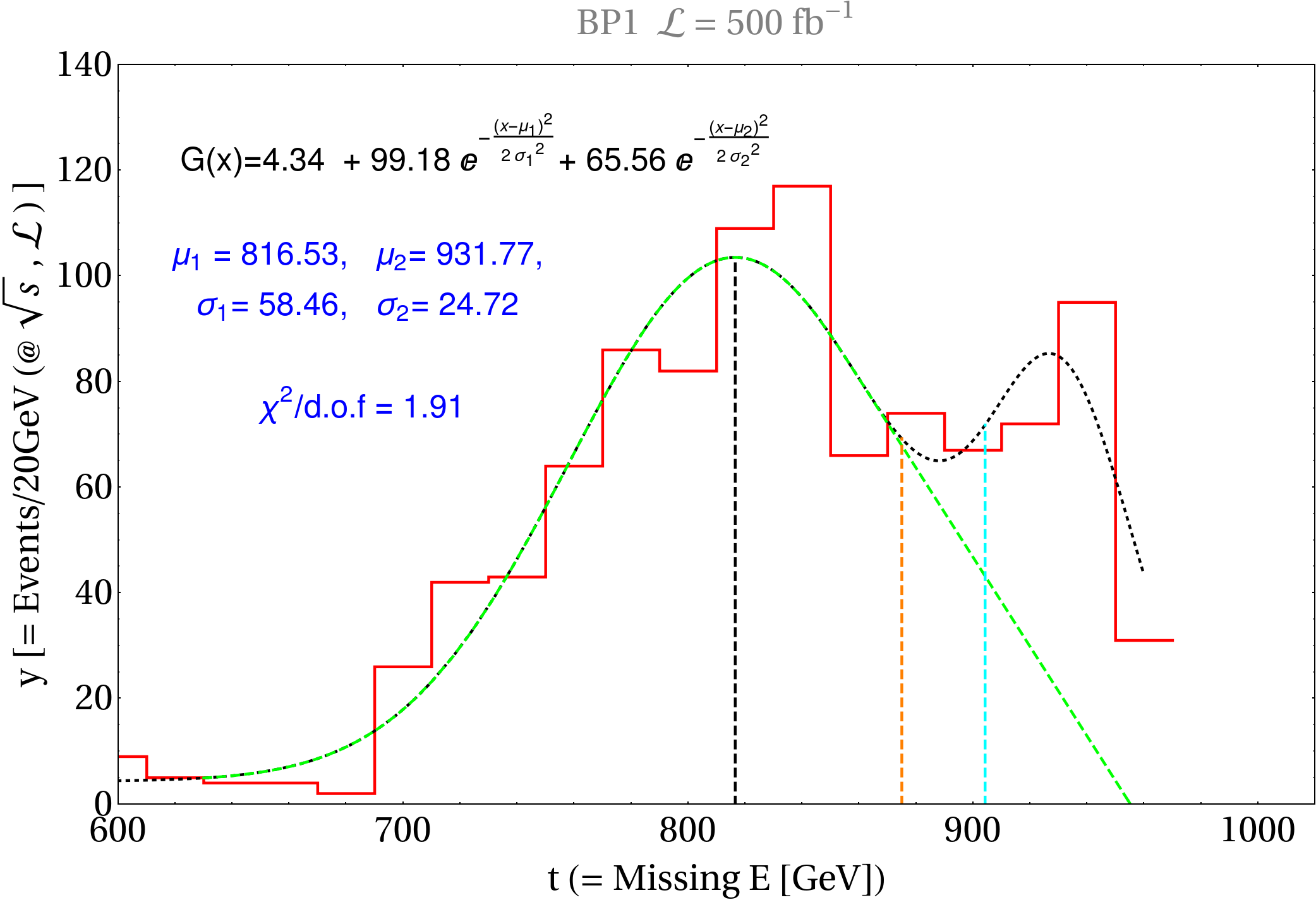
(a)

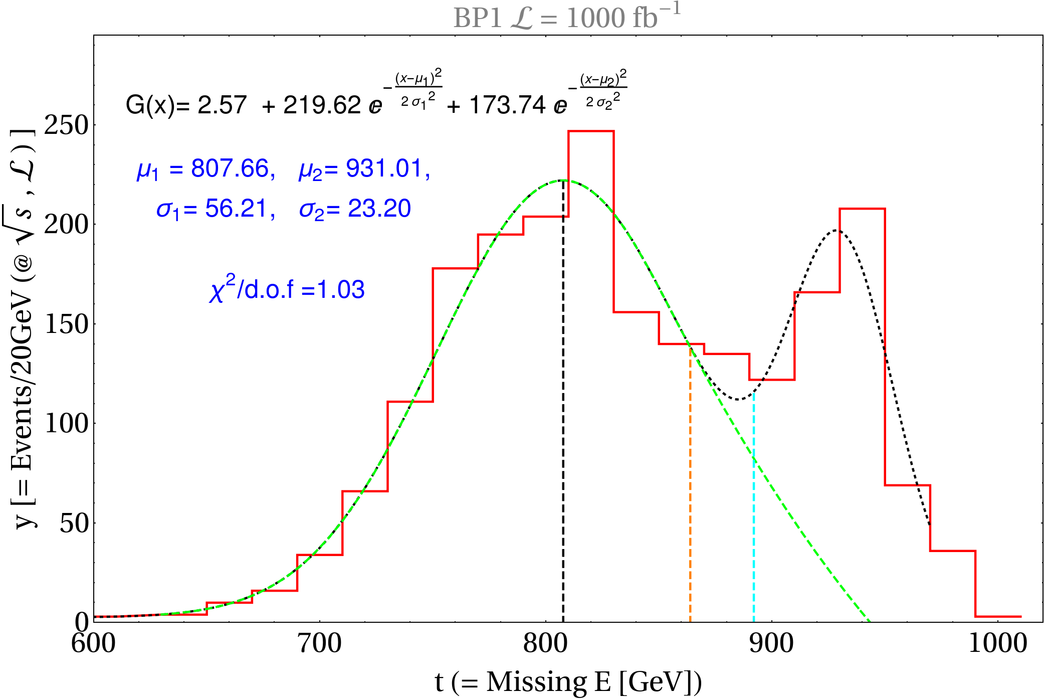
(b)

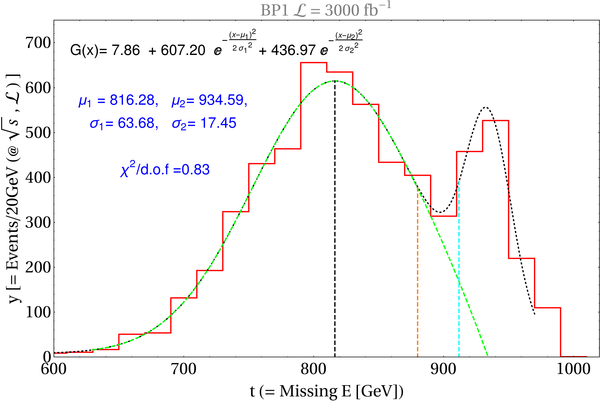
(c)

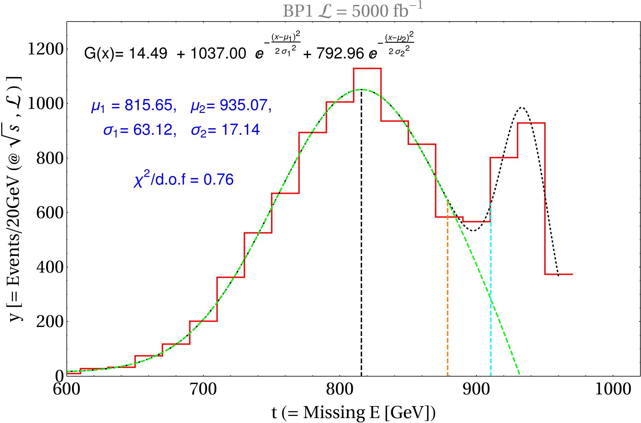
(d)

Figure 17: Gaussian Fitting of $\not{E}$ distribution for signal (BP1) plus SM background for different $\mathcal{L}$. The polarization of initial beams are chosen to be P3.

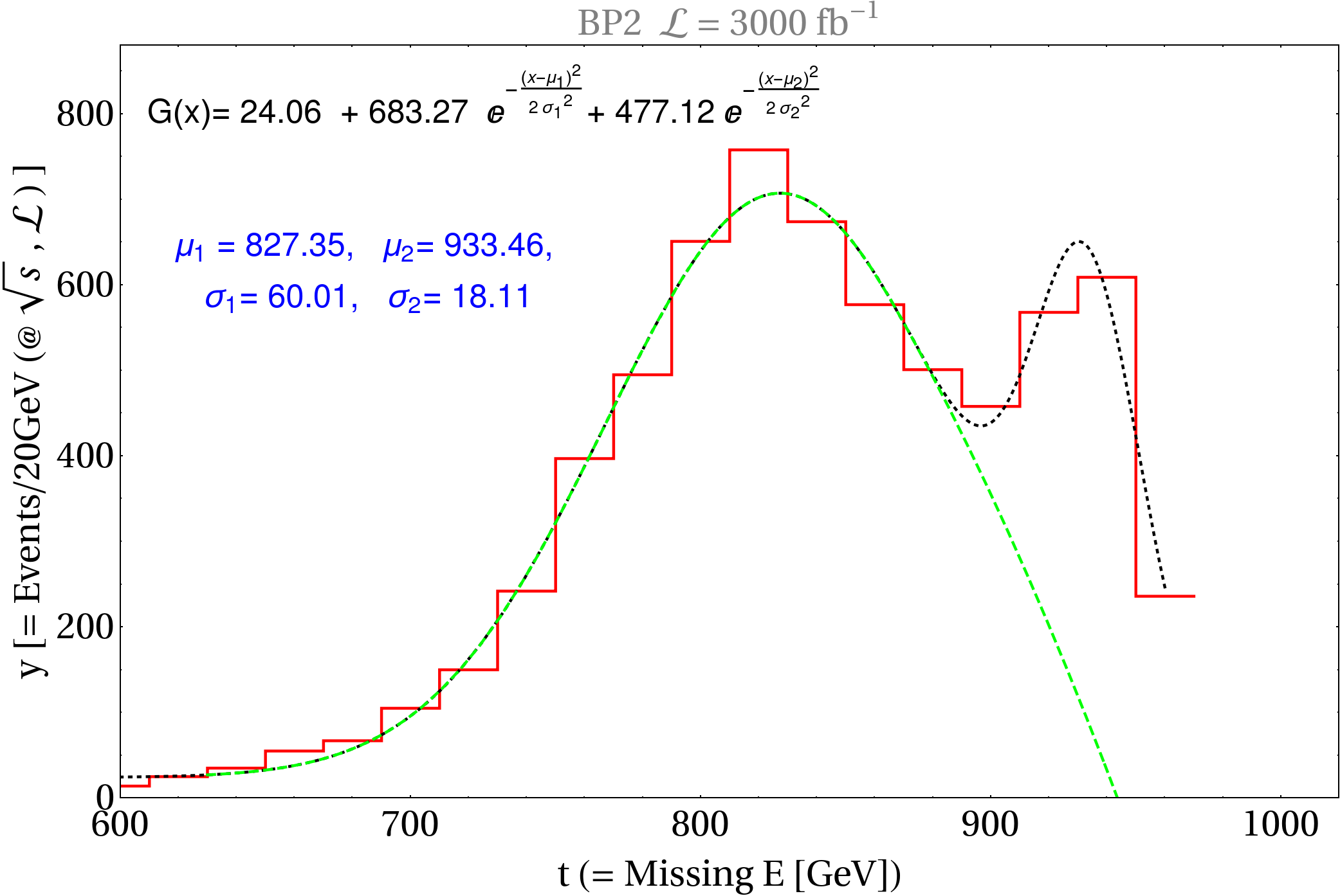
(a)

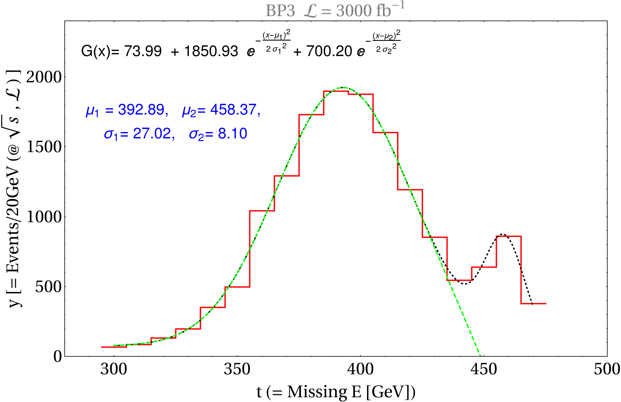
(b)

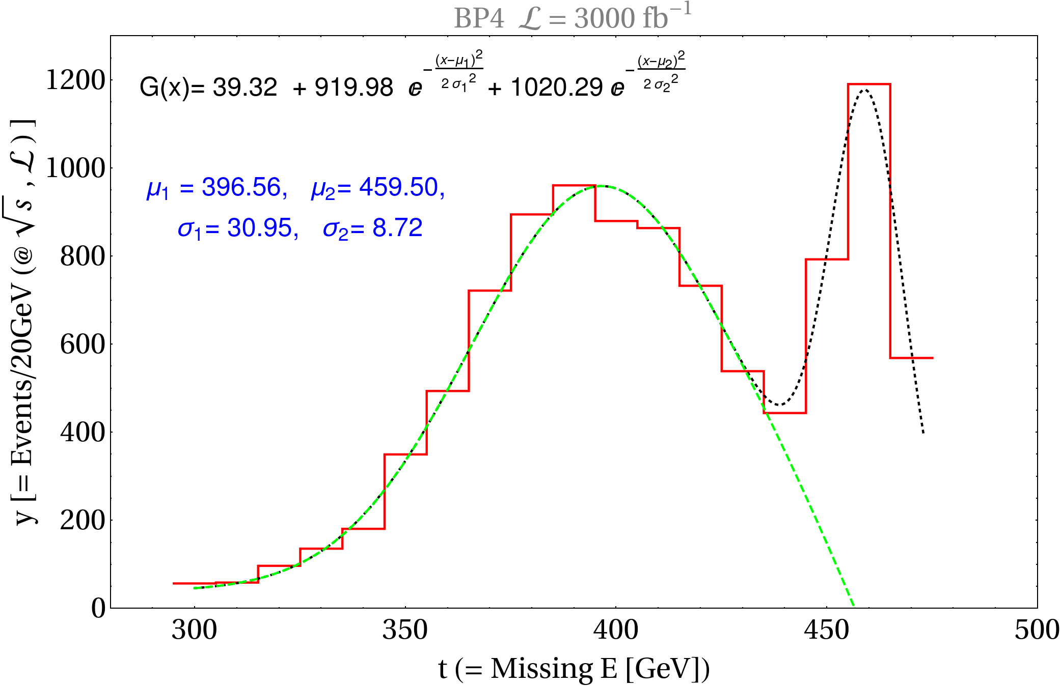
(c)

Figure 18: Same as Fig. 17 for BP2 (a), BP3 (b) and BP4 (c) at $\mathcal{L}=3000~{}{\rm fb}^{-1}$.

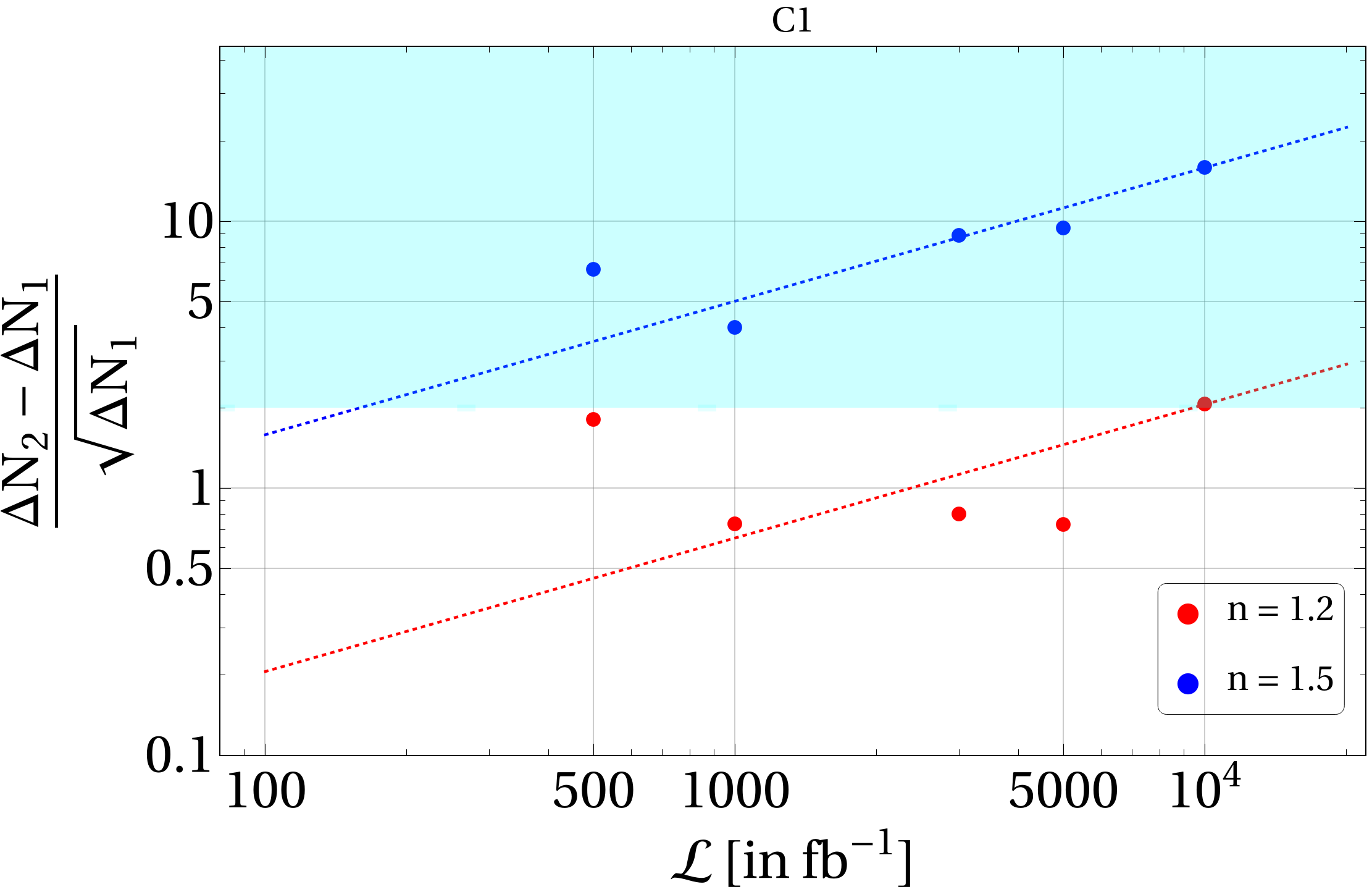
(a)

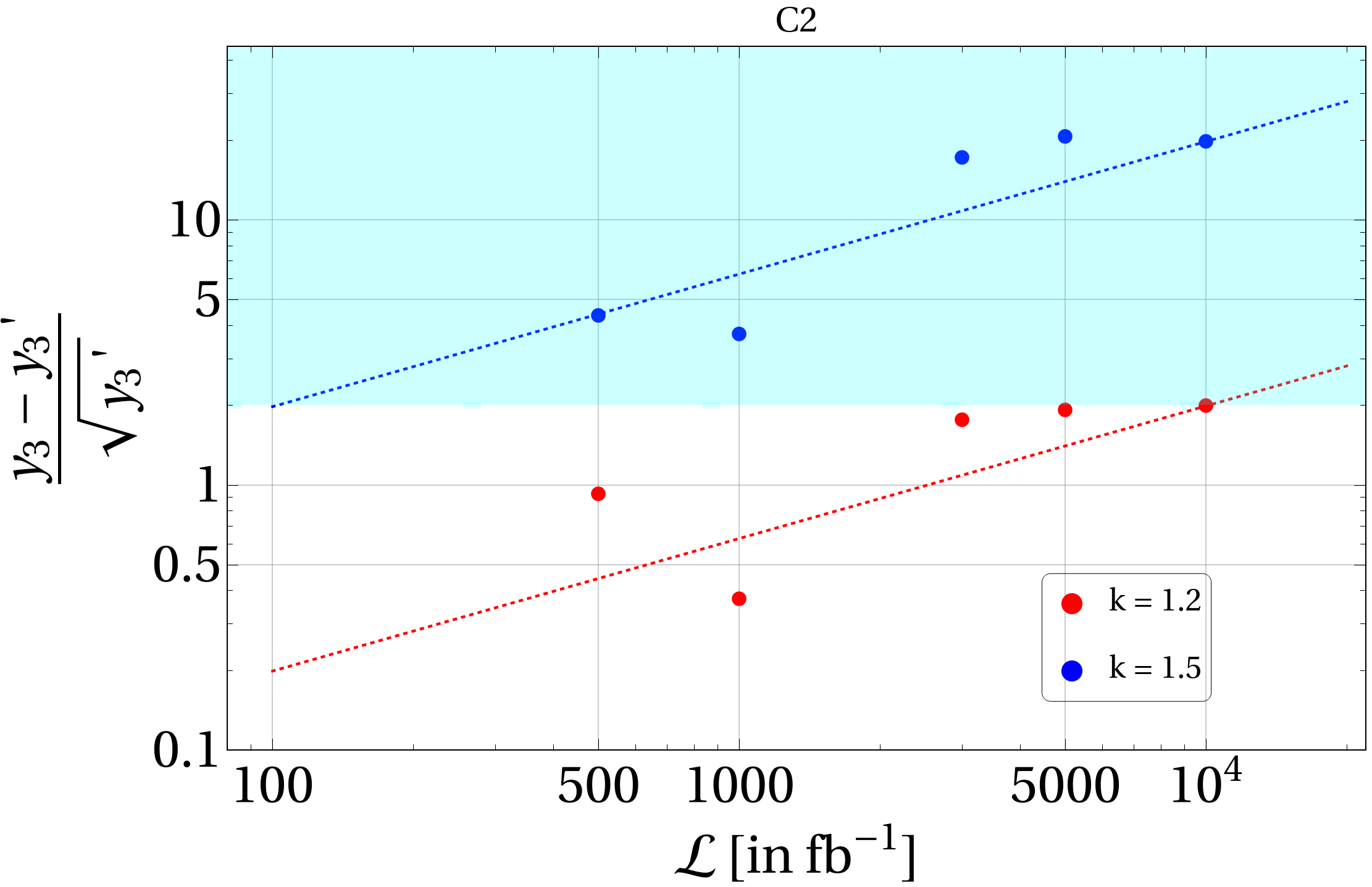
(b)

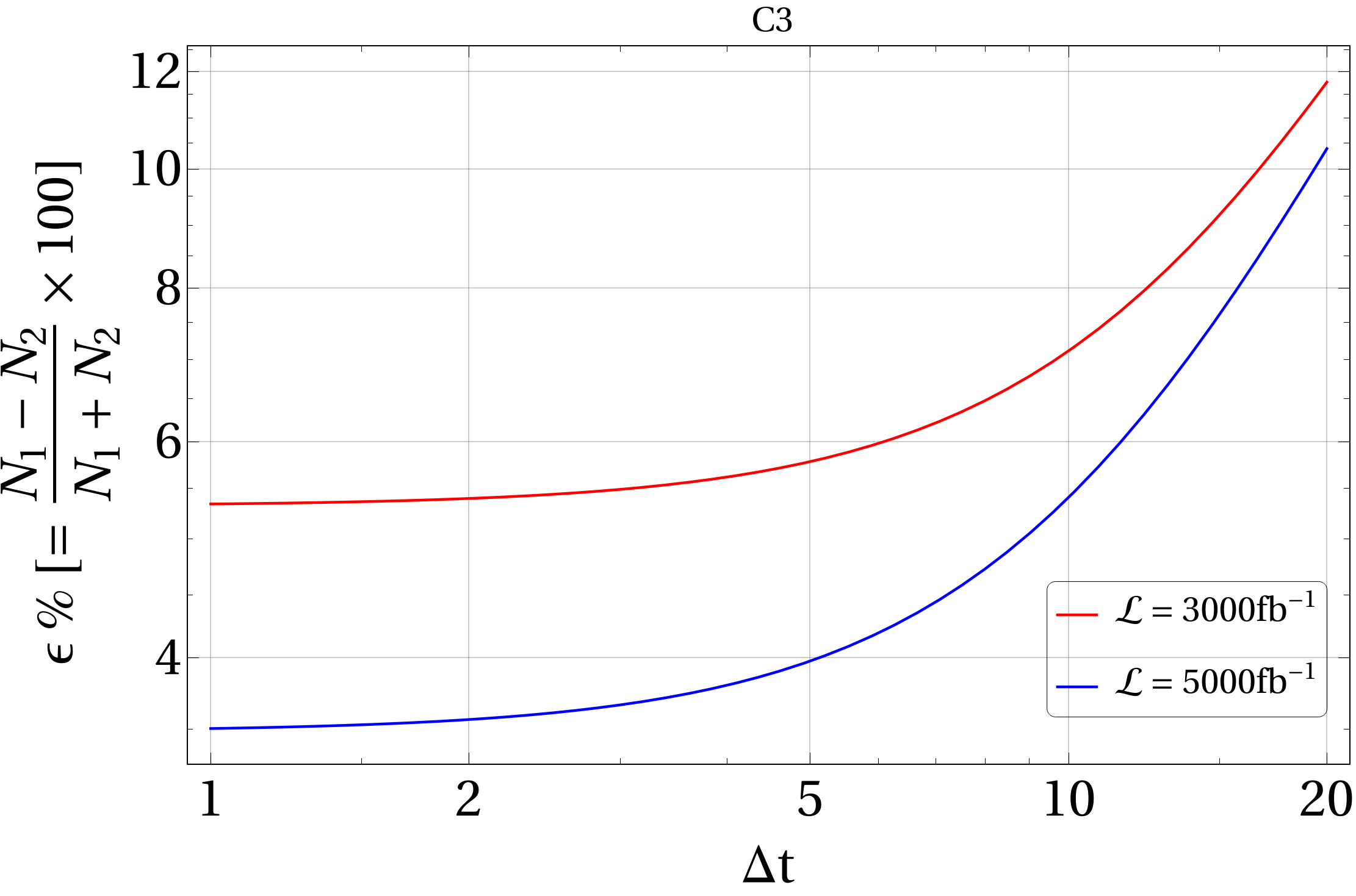
(c)

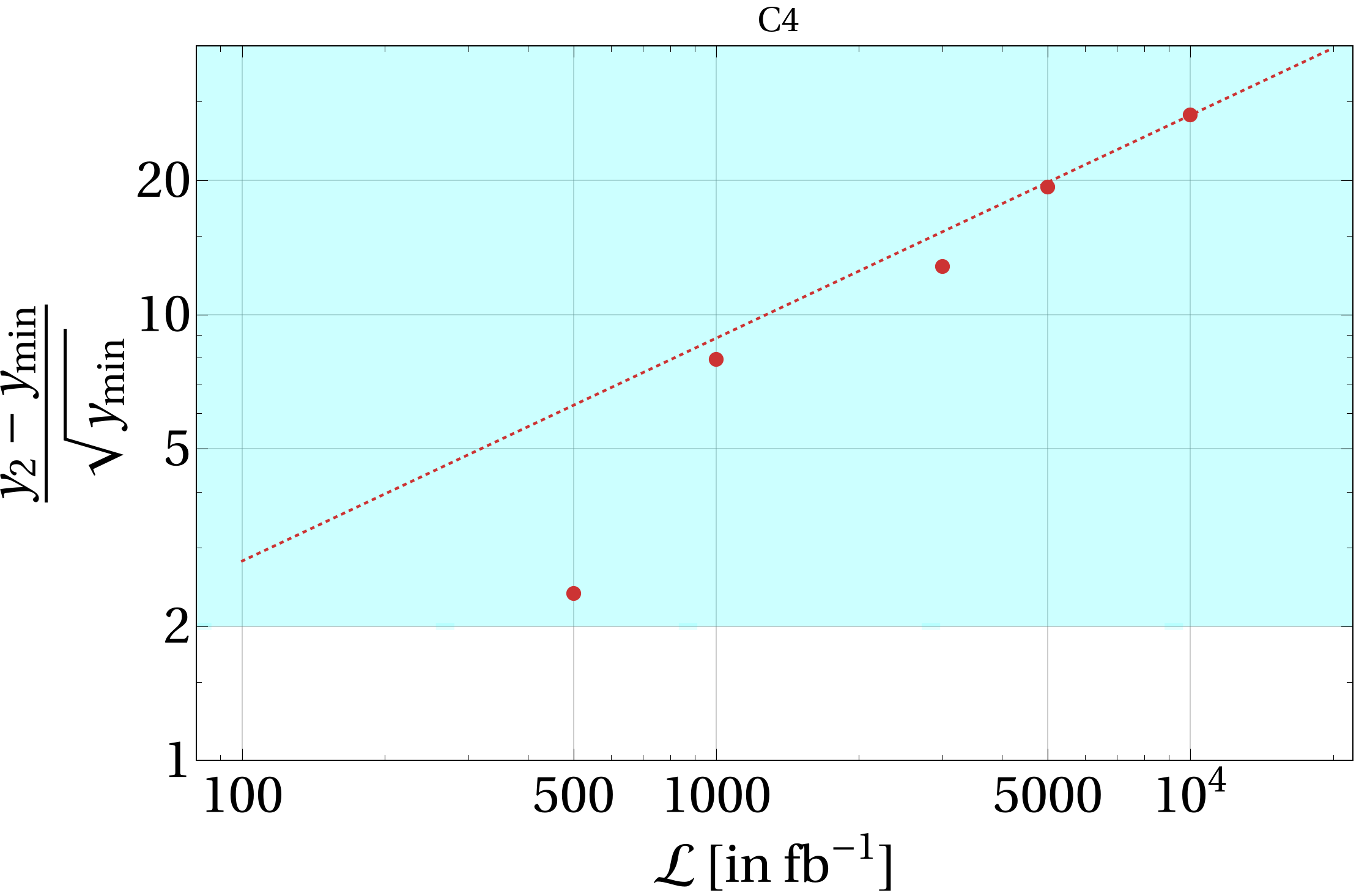
(d)

Figure 19: Statistical conditions to distinguish the two peaks for BP1: (a) $R_{C1}$ as a function of ${\mathcal{L}}$ for different $n$ (defined in Equation 31), (b) $R_{C2}$ vs $\mathcal{L}$ for different $k$ (defined in Equation (32)), (c) $R_{C3}$ as a function of $\Delta t$ (defined in Equation (33)) and (d) $R_{C4}$ vs. $\mathcal{L}$ (defined in Equation (34)). Sky blue shaded region indicates $R_{C1,2,4}>2$. The dots indicate simulated points whereas the dotted line indicates scaling with integrated luminosity as $\sim\sqrt{\mathcal{L}}$.

(a)

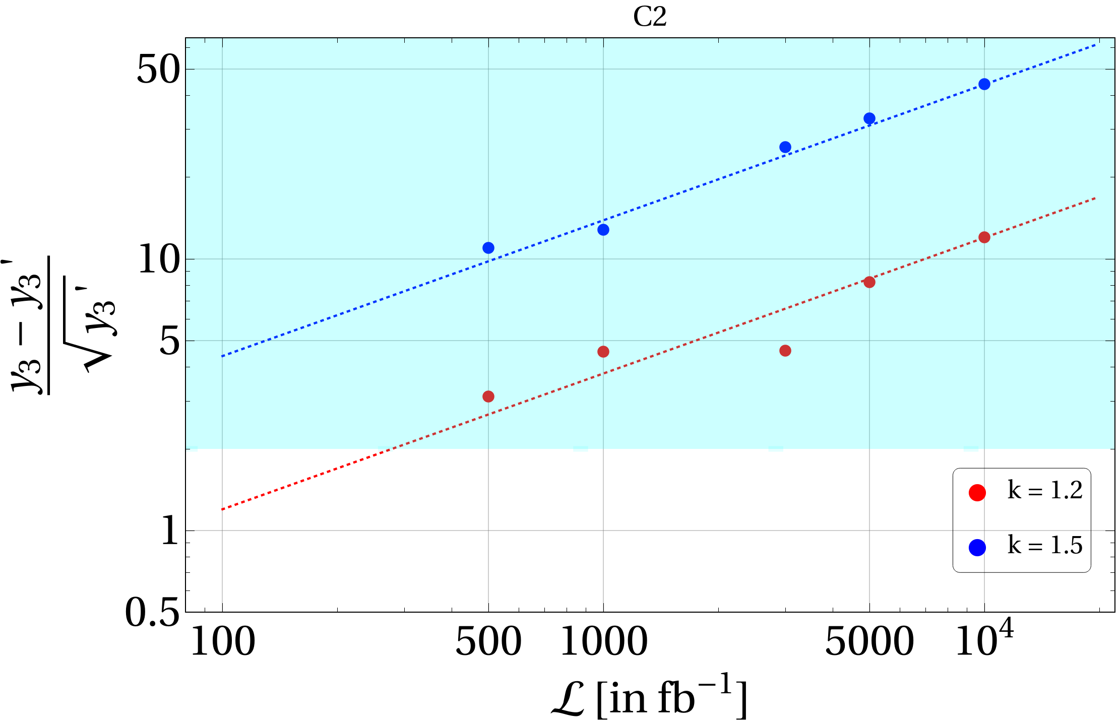
(b)

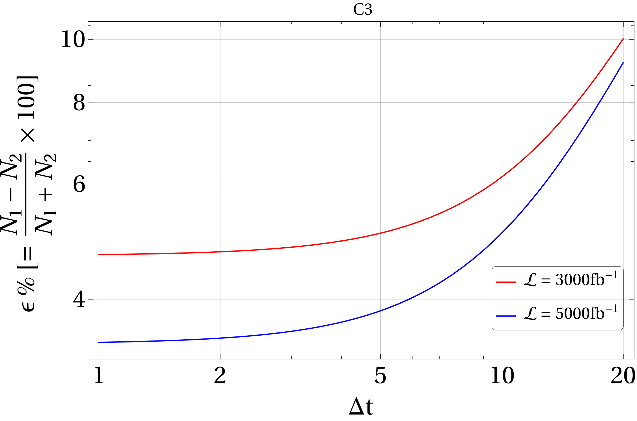
(c)

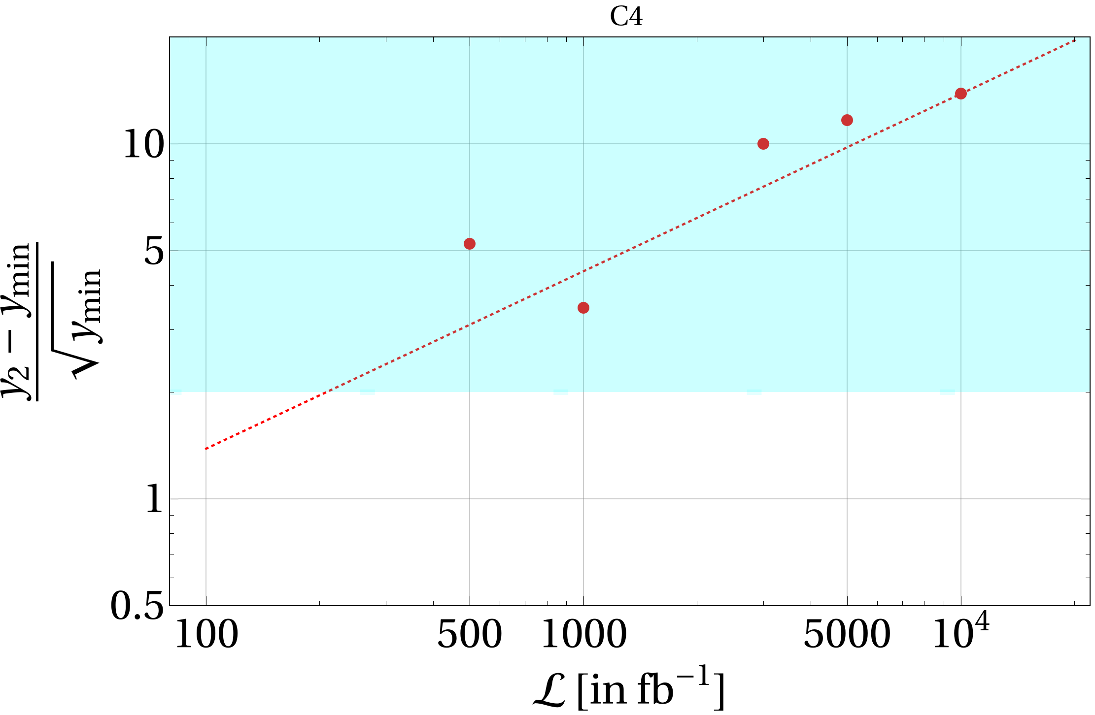
(d)

Figure 20: Same as Fig. 19 but for BP2.

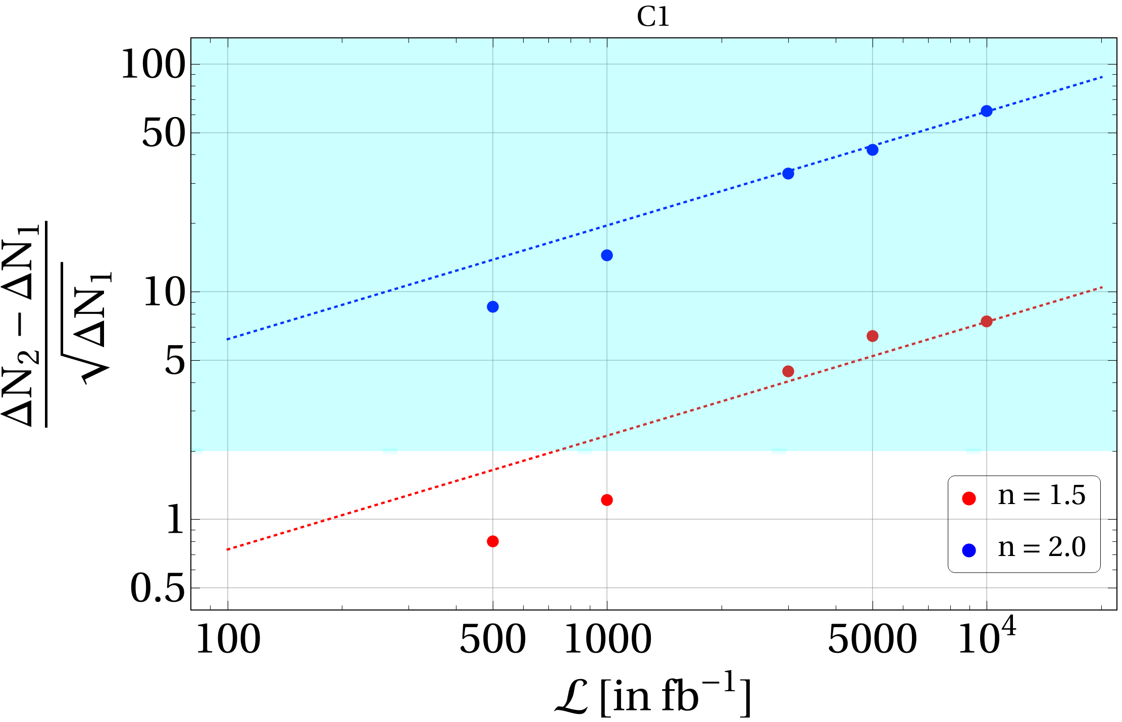
(a)

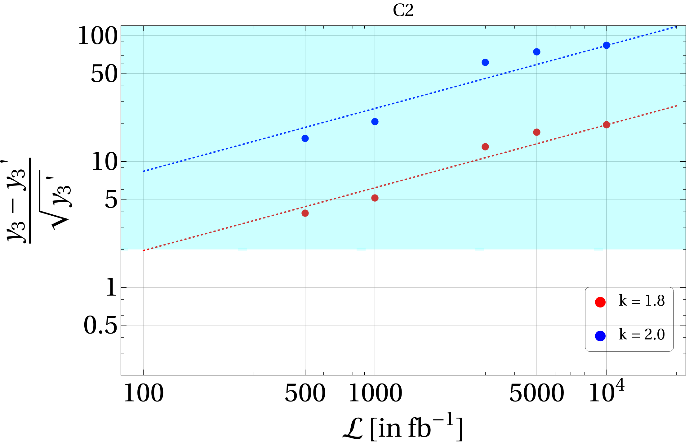
(b)

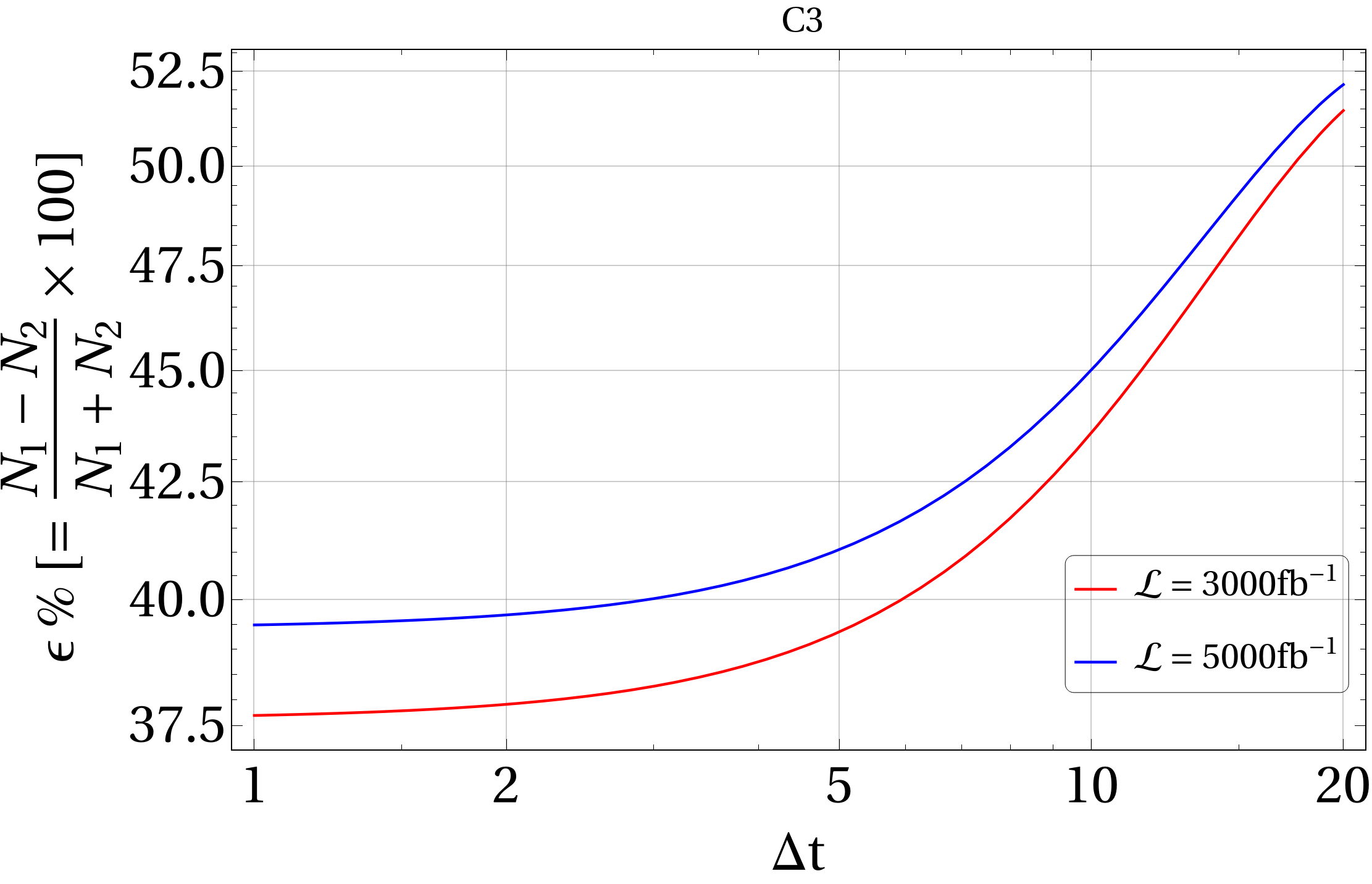
(c)

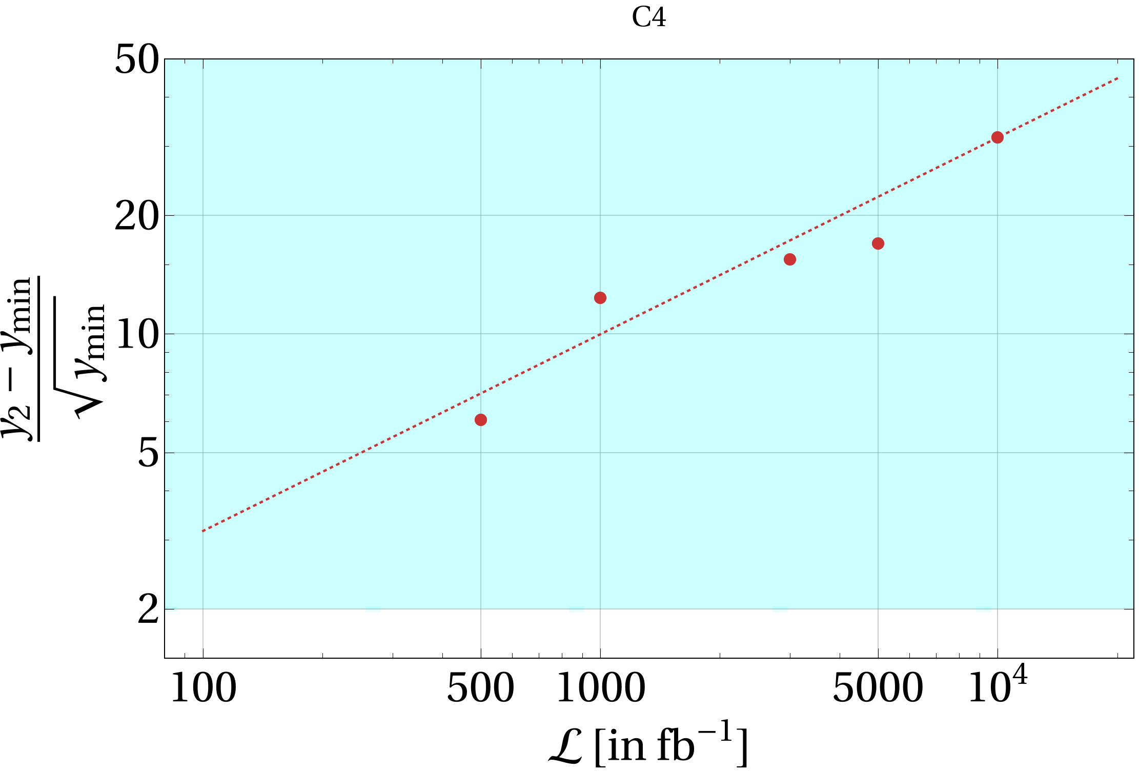
(d)

Figure 21: Same as Fig. 19 but for BP3.

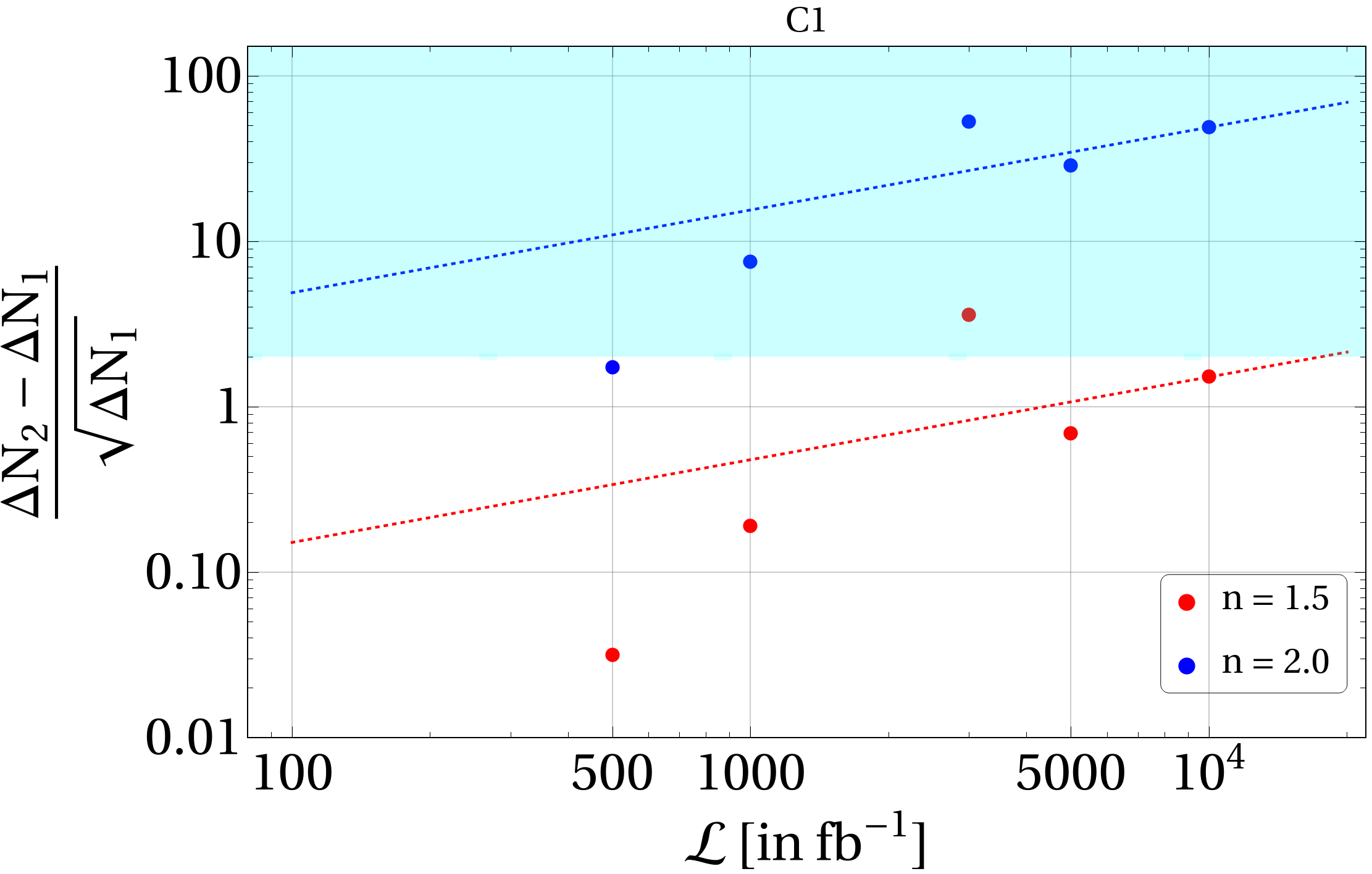
(a)

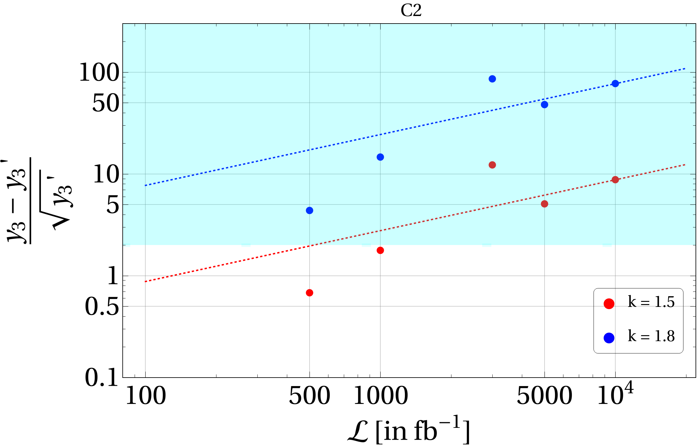
(b)

(c)

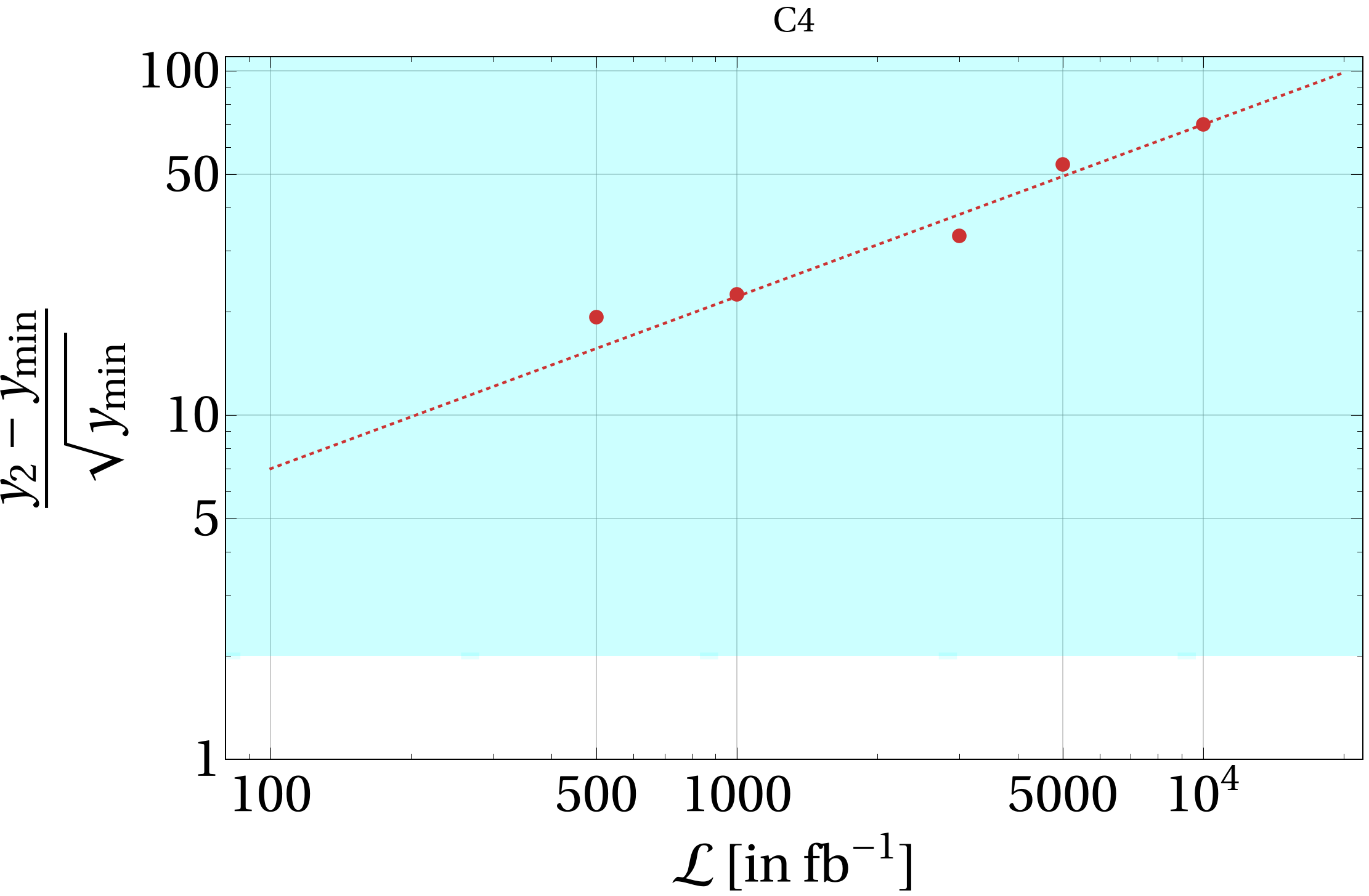
(d)

Figure 22: Same as Fig. 19 but for BP4.

The resulting $\not{E}$ distribution for BP1 along with Gaussian fits are shown in Fig. 17 for various benchmark luminosities. Those for BP2, BP3 and BP4 are provided in Fig. 18 in the left, right and bottom panel figures for a fixed $\mathcal{L}=3000~{}{\rm fb}^{-1}$. All the relevant parameters like $\mu_{1,2}$, $\sigma_{1,2}$ and $A_{1,2}$ for the Gaussian fit (following Eq. (28)) are mentioned in the figure inset. The goodness of the fit is revealed from the parameter $\chi^{2}$ as well as $\chi^{2}$ per degrees of freedom, which are also mentioned in Fig. 17. Further details on the Gaussian fitting methodology along with $\chi^{2}$ evaluation can be found in Appendix C. One can see that at low luminosities, meagre statistics leads to larger fluctuations in the distributions, and in the resulting accuracy of Gaussian fitting. They get better with higher luminosities; for example, $\chi^{2}$ per degrees of freedom in Fig. 17(a) with $\mathcal{L}=500~{}{\rm fb}^{-1}$ is 1.91, while in Fig. 17(d), with $\mathcal{L}=5000~{}{\rm fb}^{-1}$, it turns out to be 0.76.

We are now all set to discuss the conditions for distinguishing two peaks in each of these cases. In Fig. 19, we analyse BP1 in details. Fig. 19 (a) shows validation of C1 condition by plotting $R_{C1}$ as a function of integrated luminosity $\mathcal{L}$ for different values of $n$. The dots indicate the simulated points. Assuming that the point with highest luminosity provides the most accurate value of $R_{C1}$, we have scaled for other luminosities as $R_{C1}\sim\sqrt{\mathcal{L}}$ by the fitted line (which appears as a straight line in the log-log plot). The sky-blue shaded region where $R_{C1}>2$, can be achieved for $n=1.5$ with a moderate luminosity ($\mathcal{L}\sim 500~{}{\rm fb}^{-1}$). This indicates a very prominent presence of a second peak within $1.5\sigma$ vicinity of the first one. It is obvious that $R_{C1}$ increases with $\mathcal{L}$ as statistics enhance (evident from Eqn. (31)); $R_{C1}$ also increases with $n$ as we approach the second peak. In Fig. 19(b) we examine condition C2, where $R_{C2}$ is plotted as a function of $\mathcal{L}$ for various $k$ values. Again, we see that the sky-blue shaded region where $R_{C2}>2$, is achieved for $k=1.5$ with moderate luminosity. This means, number of events accumulated in $k=1.5\sigma$ apart from the first peak is larger than the number of events without the presence of the second peak by 2$\sigma$ or more. Again, as we go further away from the first peak, i.e. the larger the $k$ is, the larger $R_{C2}$ becomes. The dependence of $R_{C2}$ on $\mathcal{L}$ is obvious, the larger is $\mathcal{L}$, the easier it is to sense the presence of a second peak. In Fig. 19(c), we show the variation of $R_{C3}$ as a function $\Delta t~{}(\equiv\Delta\not{E})$ for two representative luminosities. One can see that $R_{C3}$ remains almost constant for a small range of $\Delta t$, as indicated by Eqn. (33), which actually marks the difference in height of the two peaks. But $R_{C3}$ starts increasing after a point, which mostly indicates the difference in the thickness of the Gaussian distributions around the peaks, instead of the difference in the heights of the peaks. Finally we verify condition C4 in Fig. 19(d), where $R_{C4}$ is evaluated as a function of $\mathcal{L}$. We see that it is easy to satisfy condition C4 than others as the difference between the number of events at the second peak and that of the minima between them easily goes beyond 2$\sigma$ ($R_{C4}>2$) even at small luminosities. The enhancement of $R_{C4}$ with $\mathcal{L}$ is also obvious. Figs. 20, 21, 22 present similar analysis for BP2, BP3 and BP4 respectively, where the features broadly remain the same.

A comparison between our chosen benchmarks in the light of the aforementioned distinction criteria is in order. $R_{C1}$ takes the largest value for BP2, since the relative height as well as the width of the second peak is large w.r.t the first peak in this case. On the other hand, $R_{C2}$ is highest for BP4, since the height of the second peak is largest there. $R_{C3}$ is largest for BP3, due to significant asymmetry in the heights of the two peaks. Consequently $R_{C1}$ and $R_{C2}$ take the lowest value for a specific $n$ and ${\cal L}$ in this case. $R_{C4}$ is maximum for BP4 due to large height and small width of the second peak. In general, BP1 performs best under C3, BP2 under C1 and BP4 under C2 as well as C4 criteria. BP3 does worse for all conditions, although C4 confirms the presence of a second peak clearly. This comparative analysis also exemplifies the qualitative distinction between the C1-C4 conditions and how each of them individually or together can be useful for distinguishing the two peaks.

(a)

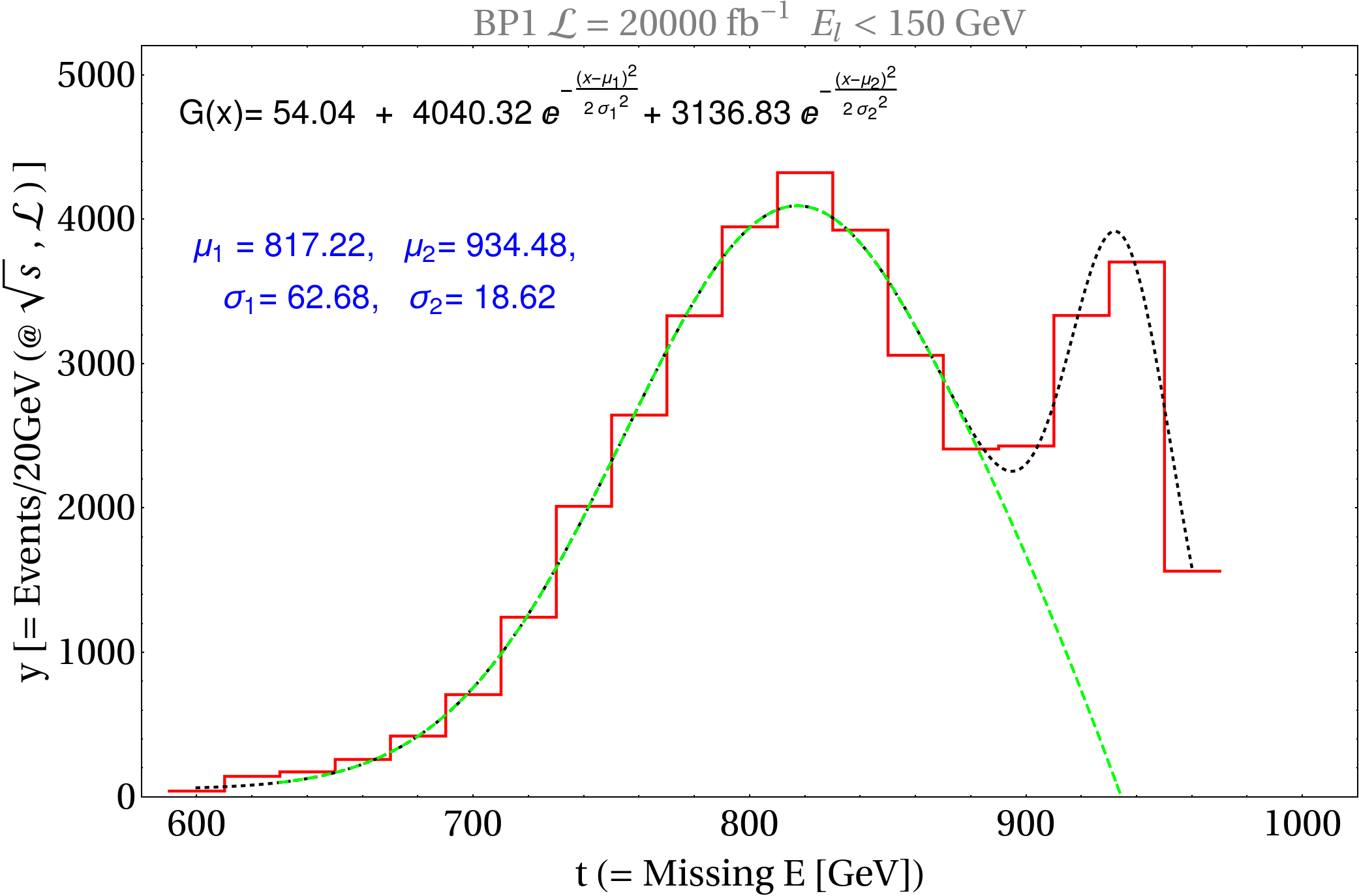
(b)

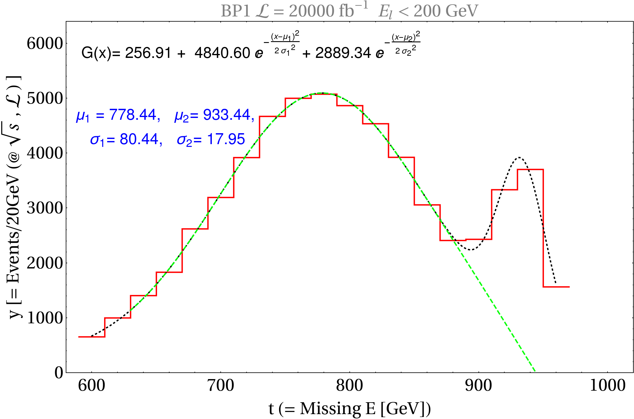
(c)

Figure 23: $\not{E}$ distribution and Gaussian fitting for BP1 together with SM background with different cuts on leading lepton energy: (a) $E_{\ell_{1}}<$ 100 GeV, (b) $E_{\ell_{1}}<$ 150 GeV and (c) $E_{\ell_{1}}<$ 200 GeV. The polarization of initial beams is chosen as P3 and $\mathcal{L}=20ab^{-1}$ has been used for illustration.

We analyse next the effect of lepton energy cut on the distinction criteria. In Fig. 23, we show $\not{E}$ distribution for BP1 together with SM background for different choices of energy cuts on the leading lepton; (a) $E_{\ell_{1}}<$ 100 GeV, (b) $E_{\ell_{1}}<$ 150 GeV and (c) $E_{\ell_{1}}<$ 200 GeV. For $E_{\ell_{1}}<$100 GeV, SM background gets reduced to a large extent. However, significant portion of the first peak of the signal also gets rejected. Consequently, the two-peak nature of the distribution disappears and only a small bump in the distribution remains. With both 150 GeV and 200 GeV cut, the reduction of background events is less but so is for the signal contribution, resulting a clear two-peak signal for both these cases. In Fig. 24, we then quantify the distinguishability of the peaks for these cases .

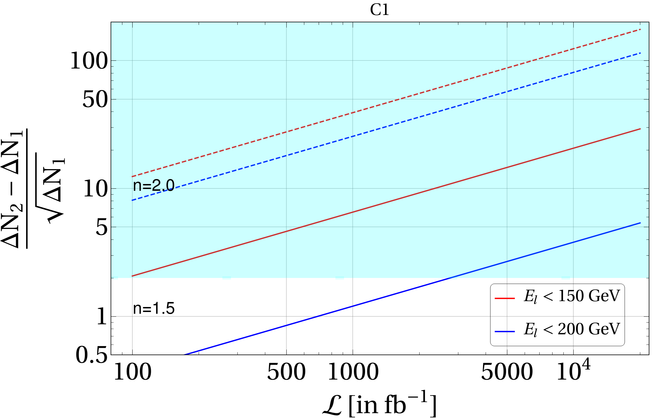
(a)

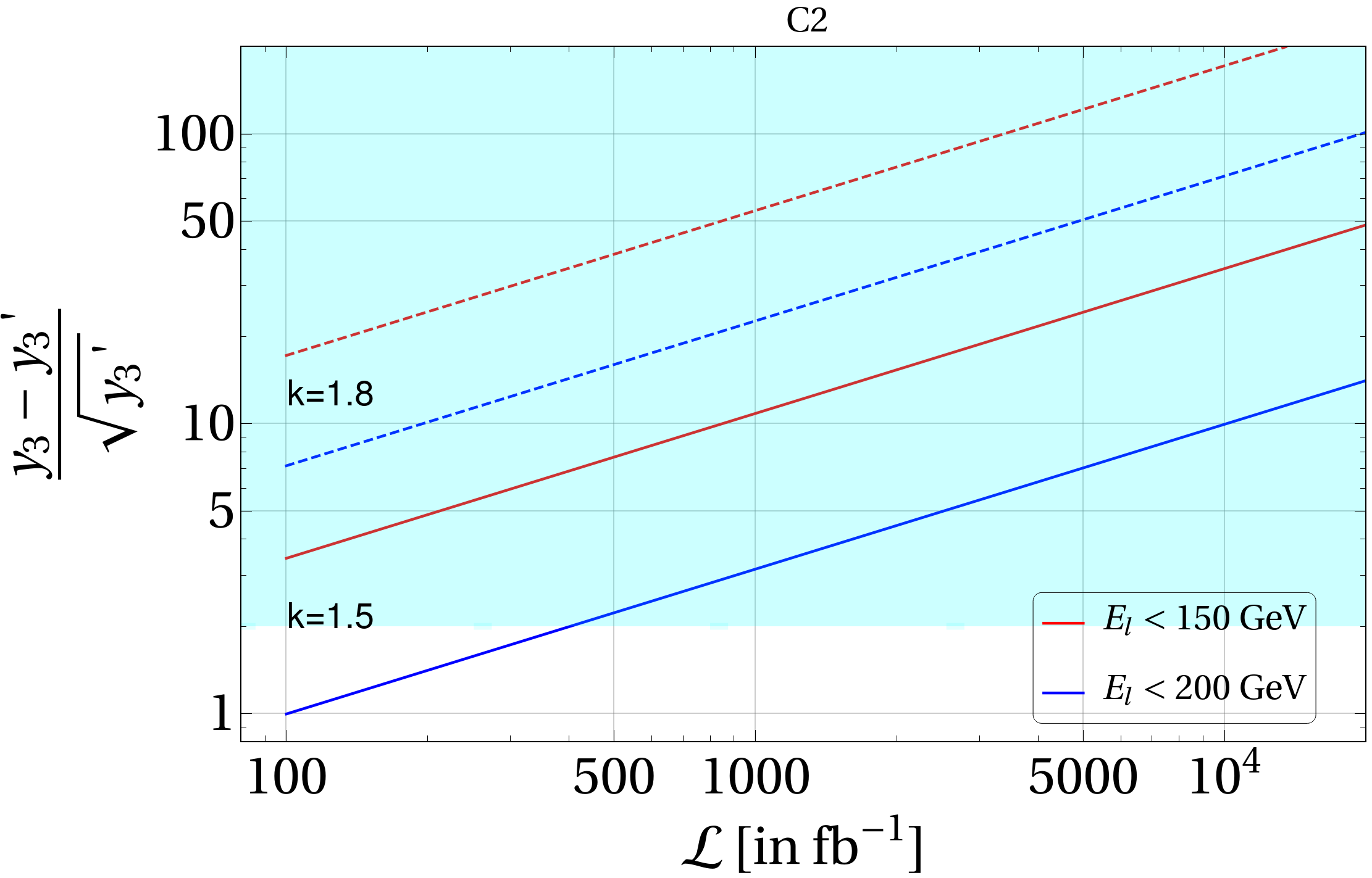
(b)

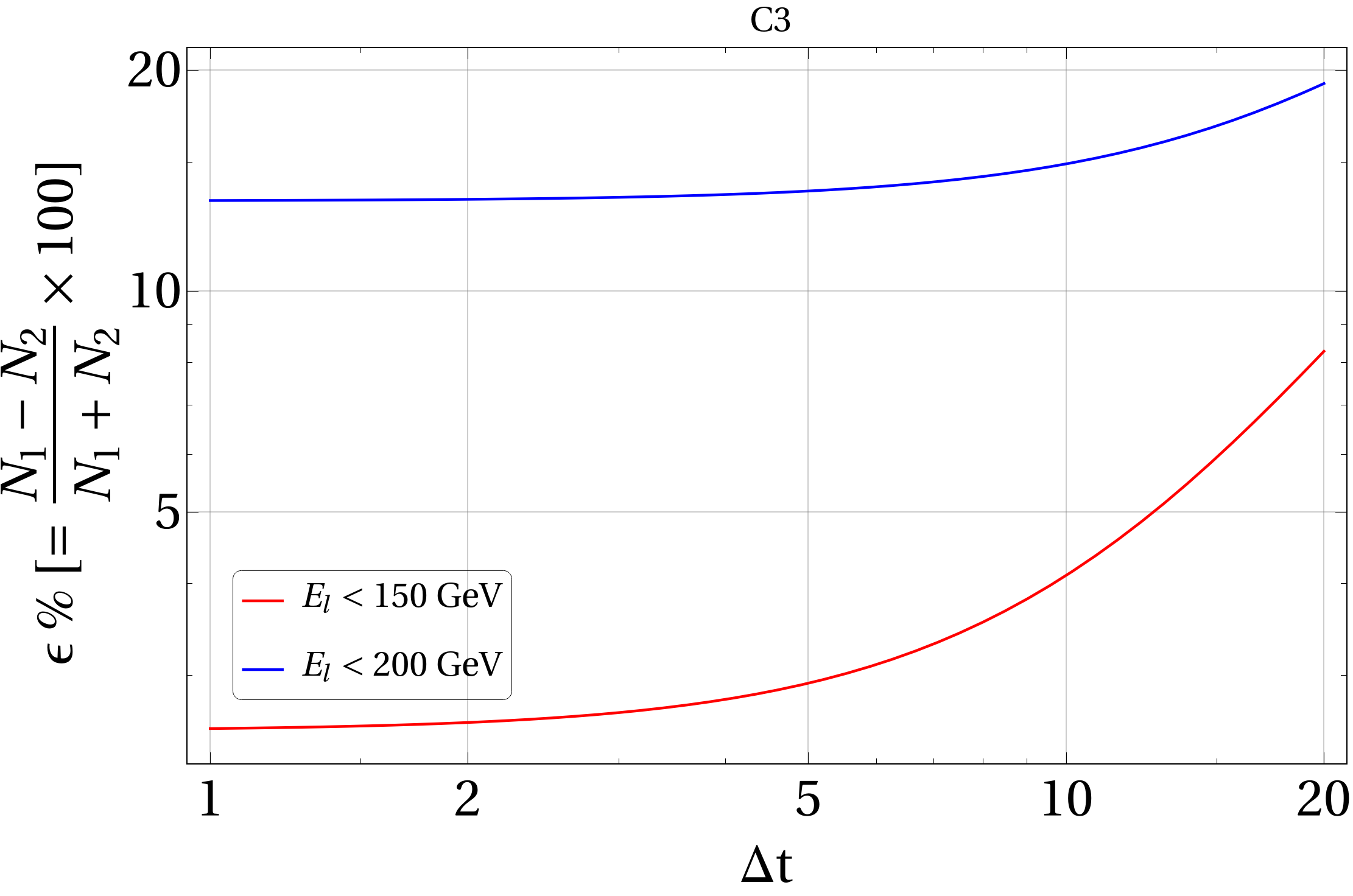
(c)

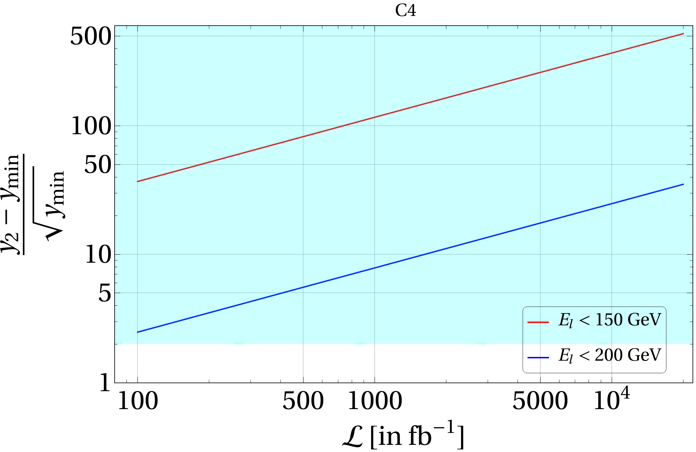
(d)

Figure 24: Validation of C1, C2, C3, C4 conditions for BP1 with two specified lepton energy cuts ($E_{\ell_{1}}<$ 150 GeV, $E_{\ell_{1}}<$ 200 GeV): (a) $R_{C1}$ as a function of $\mathcal{L}$ for different $n$ values, (b) $R_{C2}$ as a function of $\mathcal{L}$ for different $k$ values, (c) $R_{C3}$ as function of $\Delta t$ and (d) $R_{C4}$ as a function of $\mathcal{L}$.

The top panel of Fig. 24 investigates condition C1, middle panel evaluates C2, while the lower panel figures study conditions C3 and C4. One can see that at a given luminosity one has to choose higher $n(k)$ in order to get same $R_{C1}(R_{C2}$) values with $E_{\ell_{1}}<$ 200 GeV as compared to $E_{\ell_{1}}<$ 150 GeV. This is simply because the effect of second peak is subdued due to large background events contributing to first peak with the milder cut of $E_{\ell_{1}}<$ 200 GeV. This is also the reason for $R_{C3}$ to be larger with $E_{\ell_{1}}<$ 200 GeV compared to the case with $E_{\ell_{1}}<$ 150 GeV (see Fig. 24(c)). $R_{C4}$ remains almost identical in both cases, as can be seen from Fig. 24(d), as the lepton energy cut do not affect the second peak much. The effect of polarisation is studied in appendix D, where we also validate all the conditions C1-C4. We see that polarisation, although necessary for reducing SM background, doesn’t alter the distinguishability of the two peaks significantly when the SM background is sufficiently suppressed.

Let us finally summarize the key findings of this section.

• Conditions C1, C2, C3, C4 which involve $R_{C1},R_{C2}$, $R_{C3}$ and $R_{C4}$ variables respectively, can successfully distinguish double peak behaviour in the $\not{E}$ spectrum arising from two component DM signal. Among them, $R_{C4}$ turns out to be the variable with widest applicability.

• All the conditions, if simultaneously satisfied, indicate a well separated and prominent second peak; although satisfying one condition is good enough to realise the presence of a second peak.

• $R_{C1},R_{C2}$ (for specific $n(k)$) and $R_{C4}$ increase with integrated luminosity $\mathcal{L}$; therefore with larger luminosity, significant $R_{C1}$ and $R_{C2}$ values can be obtained at lower $n(k)$.

• Low $R_{C3}$ is better for distinguishable second peak (unlike other variables), which increases with $\Delta t\equiv\Delta\not{E}$ and remains almost constant with integrated luminosity.

• At low luminosity, large statistical fluctuation becomes a roadblock while one tries to identify the two-peak signature in the $\not{E}$ distribution.

• The distinction criteria are sensitive to the lepton energy cut in the chosen final state. If the cut is too stringent, the two-peak nature is lost, if the cut is too relaxed, the second peak becomes insignificant compared to the first, requiring an optimaisation.

• The distinction criteria are not too sensitive to the initial state polarization, given significant background reduction is already achieved.

• If the contributions from both the DM components overlap significantly with each other or one contribution wins over the other completely, our proposed methods will not work, since in those cases, it will be similar to single-peak distribution.

8 Summary and conclusion

We have suggested some methods of distinguishing two DM components, both of which can be pair-produced in separate events at a collider. In particular, we study a scenario with two separate dark sectors, each capable of pair-producing HDSPs, which finally decay into DM pairs of either kinds via cascades. This results in double peaks in $\not{E}$ or $\not{E}_{T}$ distributions, whose identification and segregation constitute the quintessence of our investigation.

The key variables that play a role in producing distinguishable peaks are both of the DM masses ($m_{\rm DM_{1}},m_{\rm DM_{2}}$) and their mass-splitting with the corresponding HDSPs ($\Delta m_{1},\Delta m_{2}$). We further demonstrate that, while $\not{E}_{T}$ is the canonical label of invisible particles at hadron colliders, it is in $\not{E}$-distributions that the peaks are likely to be more prominent. This is because the DM masses do not play a role in $\not{E}_{T}$, while they show up in the $\not{E}$-distribution, thus making the peaks more distinct, when the masses of the two DM-components are well-separated. Thus $e^{-}e^{+}$ colliders that have both the DM components within their kinematic reach emerge as their best hunting grounds. In addition, the absence of QCD backgrounds as well as the possibility of beam polarisation serves to reduce the background to the DM signals. All these have been illustrated in the context of a two-component DM scenario, with one scalar and one spin-1/2 DM, each being the lightest state in a separate dark sector. Relic density and direct search constraints play an important role to shrink the allowed parameter space of the model for collider study, as we have demonstrated. It is further emphasized that, unless both the dark sectors lead to similar production rates for the corresponding DM pairs, the peak of one may get buried under the other. We have demonstrated, with appropriate benchmarking, how this requirement carves out identifiable regions in the dual-DM parameter space at an electon-positron collider with a given centre-of-mass energy.

We show further that the $WW$ background to $\ell^{+}\ell^{-}+\not{E}$ signal can either spoil or highlight the double-hump behaviour in the $\not{E}$ distribution. We recommend the use of right-polarised electron beams and left-handed positron polarisation to reduce the $WW$ background contamination. A judicious cut on the lepton energy may help in keeping background $WW$ peak coincide nearly with one of the DM peaks.

Finally, we offer some prescriptions for distinguishing the two peaks in the $\not{E}$ distribution. For this purpose, we suggest a set of criteria which quantify the height, sharpness and separability of one peak relative to the other. We also indicate the integrated luminosities which make these criteria useful, keeping the SM background in consideration. Some of these criteria can be useful even in cases where one goes beyond the cascading dark sector mode of dual-DM production Bhattacharya:2022qck . These distinguishability criteria are seen to be rather mildly sensitive to beam polarisation, once the SM background reduction has been achieved; on the other hand, they depend on the lepton energy cuts. On the whole, it is concluded that pushing the luminosity frontier to the level of several atobarns at an electron-positron machine is a desideratum, if one aspires to distinguish a dual-DM scenario with the available energy reach.

Appendix

Appendix A Some features of $\not{E_{T}}$, $\not{E}$ and $\not{M}$

In the limit of $\sqrt{s}\simeq 2m_{\rm HD}$, HDSPs are produced almost at rest, decays further to SM fermion ($f$) and DM. Energy momentum conservation yields,

$$|\vec{p}_{\rm DM}|=|\vec{p}_{f}|,~{}~{}~{}E_{\rm DM}+E_{f}=m_{\rm HD}.$$ (35)

Using equation of motion for DM (for both DMs at either end of the decay chain),

$$\sqrt{|\vec{p}_{DM}|^{2}+m_{\rm DM}^{2}}+|\vec{p}_{f}|=m_{\rm HD}.$$ (36)

Substituting $|\vec{p}_{f}|$ in terms of $|\vec{p}_{\rm DM}|$, from Equation 35,

$$\sqrt{|\vec{p}_{\rm DM}|^{2}+m_{\rm DM}^{2}}+|\vec{p}_{\rm DM}|=m_{\rm HD}\,,~{}\therefore|\vec{p}_{\rm DM}|=\frac{1}{2}\Delta m\left(1+\frac{m_{\rm DM}}{m_{\rm DM}+\Delta m}\right)\,.$$ (37)

Denoting the momenta of the DM pair as $|\vec{p}^{1}_{\rm DM}|$ and $|\vec{p}^{2}_{\rm DM}|$, the angle between them as $\theta$, $\not{E_{T}}$ can be written as,

$$\not{E_{T}}=\sqrt{|\vec{p}^{1}_{\rm DM}|^{2}+|\vec{p}^{2}_{\rm DM}|^{2}+|\vec{p}^{1}_{\rm DM}||\vec{p}^{2}_{\rm DM}|\cos\theta}\,.$$ (38)

It is maximum when $\theta=0$; i.e. the two DM particles are colinear. Therefore,

$$\not{E_{T}}^{max}=|\vec{p}^{1}_{\rm DM}|+|\vec{p}^{2}_{\rm DM}|=\Delta m\left(1+\frac{m_{\rm DM}}{m_{\rm DM}+\Delta m}\right)=\Delta m\left(1+r\right)\,;$$ (39)

where $r=\frac{m_{\rm DM}}{m_{\rm HD}}$. On the other hand, following the energies of the two DM particles as,

$$E^{1}_{\rm DM}=\sqrt{|\vec{p}^{1}_{\rm DM}|^{2}+m_{\rm DM}^{2}},~{}~{}E^{2}_{\rm DM}=\sqrt{|\vec{p}^{2}_{\rm DM}|^{2}+m_{\rm DM}^{2}}\,;$$ (40)

we get,

$$\not{E}=E^{1}_{\rm DM}+E^{2}_{\rm DM}=\sqrt{|\vec{p}^{1}_{\rm DM}|^{2}+m_{\rm DM}^{2}}+\sqrt{|\vec{p}^{2}_{\rm DM}|^{2}+m_{\rm DM}^{2}}\,.$$ (41)

Let us now turn to $\not{M}$. We plot the normalised $\not{M}$ distribution in Fig. 25 for the pair production of the charged component of the inert scalar doublet with fixed $m_{\rm DM}$ and different $\Delta m$, where the peak shifts to the left with larger $\Delta m$. For hadronically quiet signals $\not{M}$ becomes,

$$\not{M}=\sqrt{\not{E}^{2}-|{\sum_{i}}~{}\vec{p}_{\ell_{i}}|^{2}}\,.$$ (42)

Evidently, $\not{M}$ distribution turns similar to $\not{E}$ distributions, and does not offer much advantage in our context, unless $|{\sum}\vec{p}_{\ell_{i}}|$ is very large. However, such a situation can rarely occur for current planned $e^{+}e^{-}$ colliders. We consider a few situations to illustrate the same,

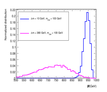
Figure 25: Normalised $\not{M}$ distribution for two cases with same DM mass and different $\Delta m$ (see figure insets for details). The production and decay chain remains similar to that of Fig. 2.

• ${\Delta m}=10$ GeV and $m_{\rm DM}=50$ GeV

  In this case, HDSP mass is low, so that the HDSPs are produced with significant boost. Therefore, the lepton and DM are almost collinear, while the two leptons are almost back-to-back for conservation of four-momenta. The effective visible momenta (second term in Eqn. 42) is negligibly small, resulting almost overlapping $\not{M}$ and $\not{E}$ distributions as shown in left hand side of Fig. 26. A similar situation arises when HDSP mass is heavy with a reasonable large DM mass. Then the lepton momenta itself is negligible, producing similar $\not{E}$ and $\not{M}$ distributions.

  

  

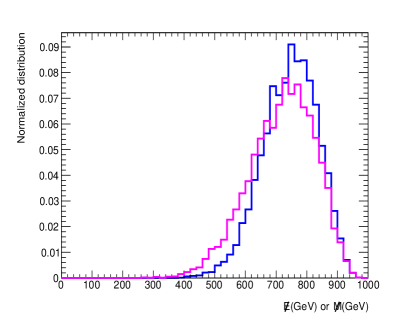
  Figure 26: Comaparison between $\not{E}$ (blue) and $\not{M}$ (pink) distribution for Left: $\{\Delta m,m_{\rm DM}\}=\{10,50\}$ GeV, Right: $\{\Delta m,m_{\rm DM}\}=\{450,20\}$ GeV.

• ${\Delta m}=450$ GeV and $m_{\rm DM}=20$ GeV

  We consider next a scenario where, HDSP is massive and therefore produced almost at rest. In such cases, momenta of the lepton and DM produced at each end will almost fully cancel each other. Therefore, the leptons are not necessarily produced back to back. However, the DM being very light ensures the magnitudes of lepton momenta are substantial. Therefore, in this case $\not{M}$ distribution shows the maximum noticeable departure from the $\not{E}$ distribution. The deviation is however largest at the left tail-end (although   $<$ [-0.07cm] $\sim$   10%) as can be seen from the right hand plot of Fig. 26.

It is possible to a have discernible difference between $\not{E}$ and $\not{M}$ distributions when leptons have considerable energy and are not back to back. At limited centre of energy of ILC such situations are rare to occur. But with high energy muon-colliders such a situation can arise and the two distributions can be significantly different.

Appendix B Annihilation, co-annihilation and elastic scattering of DM

Figure 27: Feynman diagrams for DM annihilation to SM particles for the Scalar DM ($\phi^{0}$).

Figure 28: Feynman diagrams for DM co-annihilation to SM particles for the Scalar DM ($\phi^{0}$) associated with heavy states ($A^{0},\phi^{\pm}$).

Figure 29: Feynman diagrams for DM annihilation to SM particles for the Fermion DM ($\psi_{1}$).

Figure 30: Feynman diagrams for DM co-annihilation to SM particles for the Fermion DM ($\psi_{1}$) associated with the heavy states, $\psi_{2}$, $\psi_{3}$ and $\psi^{\pm}$.

Figure 31: Feynman diagrams for DM conversion between scalar and fermion DM.

The SDM ($\phi^{0}$) can annihilate and co-annihilate with other heavy states, $A^{0}$ and $\phi^{\pm}$ to SM particles via Higgs and gauge mediated interactions as shown in Fig. 27 and Fig. 28 respectively. Similarly, the FDM has Higgs and gauged mediated annihilation as well as co-annihilation processes to SM as shown in Fig. 29 and Fig. 30 respectively. Along with the standard annihilation and co-annihilation channels, the model also yield DM-DM conversion where one DM component can annihilate into the other as shown in Fig. 31. Both the dark sectors having SM gauge interaction, naturally allows them to be in thermal bath in the early universe and behave as WIMPs. The SDM in the mass range $m_{W}\lesssim m_{\phi^{0}}\lesssim 525$ GeV provides under abundance ($\Omega_{\rm DM}h^{2}<0.12-0.001$) to form one component of the two DMs. For FDM, the gauge mediated annihilation is suppressed by the mixing angle $\sin\theta$. Relic under abundace for FDM is achieved both at very low $\Delta m_{2}$ via co-annihilation and at large $\Delta m_{2}$ ($\propto Y$) where Higgs-mediated annihilation provide required depletion.

Figure 32: Feynman diagrams for spin independent DM-neucleon scattering process for scalar and fermion DM.

Both the scalar ($\phi^{0}$) and fermion ($\psi_{1}$) DM can be detected through Higgs mediated $t-$ channel spin-independent (SI) DM-neucleon scattering events, as depicted in Fig. 32. At the tree-level, the DM-nucleon scattering cross-section for SDM $\sigma_{\rm SI}(\phi^{0})\propto\lambda_{L}^{2}/m_{\phi^{0}}^{2}$, while for FDM, $\sigma_{\rm SI}(\psi_{1})\propto Y^{2}/m_{\psi_{1}}^{2}$ ($Y\propto\Delta m_{2}\sin\theta$). It is clear that for FDM, large $\Delta m_{2}$ will result in large direct-detection cross-section, and therefore be disfavoured from the data, unless $\sin\theta$ is small. Such small values of $\sin\theta$ will of course lead to small annihilation and relic over-abundance. Therefore, $Z$ or Higgs resonance regions are only allowed for FDM.

Appendix C A sample benchmark from Region III

Let us examine a benchmark point BP5 from Region III, given in Table 6, where $m_{\phi^{0}}<m_{\psi_{1}}$ and $\Delta m_{1}>\Delta m_{2}$. Since the scalar HDSP has larger production cross-section compared to the fermionic HDSP, we consider $m_{\phi^{\pm}}<m_{\psi^{\pm}}$, in order to have comparable cross-section for both DM sectors. $m_{\phi^{0}}<m_{\psi_{1}}$ would imply that $\not{E}$ peak pertaining to SDM will appear on the left of the FDM peak. However the SDM peak will have smaller height and will be broader owing to large $\Delta m$. In such a case, the peak from scalar sector will be mostly buried under $WW$ tail(see Fig. 33(a)).

Benchmark	$m_{\phi^{0}}$ and $\Delta m_{1}$	$m_{\psi_{1}}$ and $\Delta m_{2}$	$\sigma$(fb)	$\sigma$(scalar)	$\sigma$(fermion)
BP5	60 GeV, 60 GeV	448 GeV, 40.0 GeV	1.5 fb	0.7 fb	0.8 fb

Table 6: Signal benchmark point and cross section for $P_{e^{-}}=0.8,P_{e^{+}}=-0.3$ polarization at $\sqrt{s}=$ 1 TeV centre-of-mass energy.

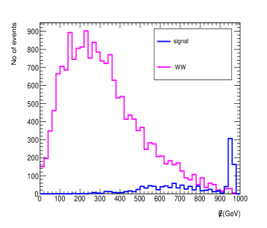
(a)

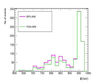
(b)

Figure 33: $\not{E}$ distribution for (a) signal (BP5) and $WW$ background, (b) (pink) signal (BP5) + $WW$ background after applying cuts and (green) single component FDM + $WW$ background after applying cuts.

The $\not{E}$ distribution in this case not only fails to produce clearly separated peaks of comparable sizes, but yields very similar distribution to the scenario, when there exists only a single DM component and the background distribution contributes to a second peak-like behaviour. In Fig. 33(b) we see, a single component FDM (pertaining to FDM sector of BP5) along with $WW$ background (green histogram), gives rise to $\not{E}$ distribution very similar to two-component DM scenario in BP5 along with $WW$ background (pink histogram). This is a rather general consequence of the lower peak from DM signal having a much flatter distribution. Although the two peaks are well-separated, the relative size of the two peaks makes it difficult to distinguish it from single-peak scenario. From the discussion above, one may thus conclude that Region III is by and large disfavored compared to Region IV, from the perspective of peak distinction.

Appendix D Gaussian Fitting methodology

  

 

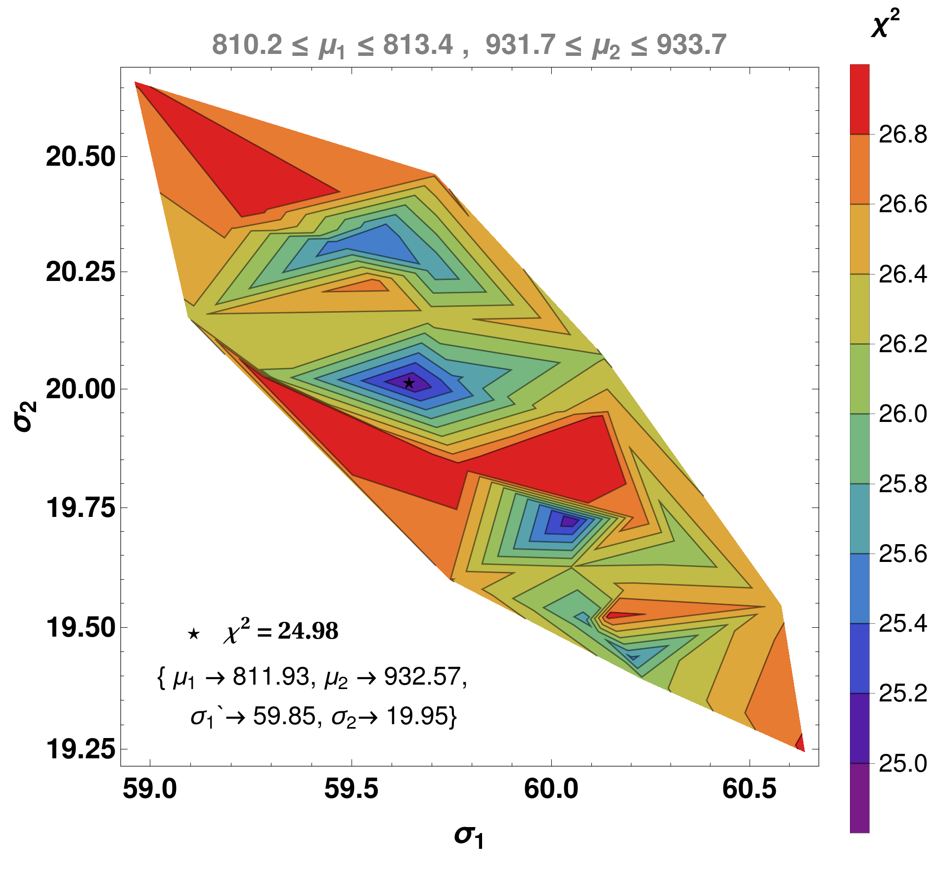
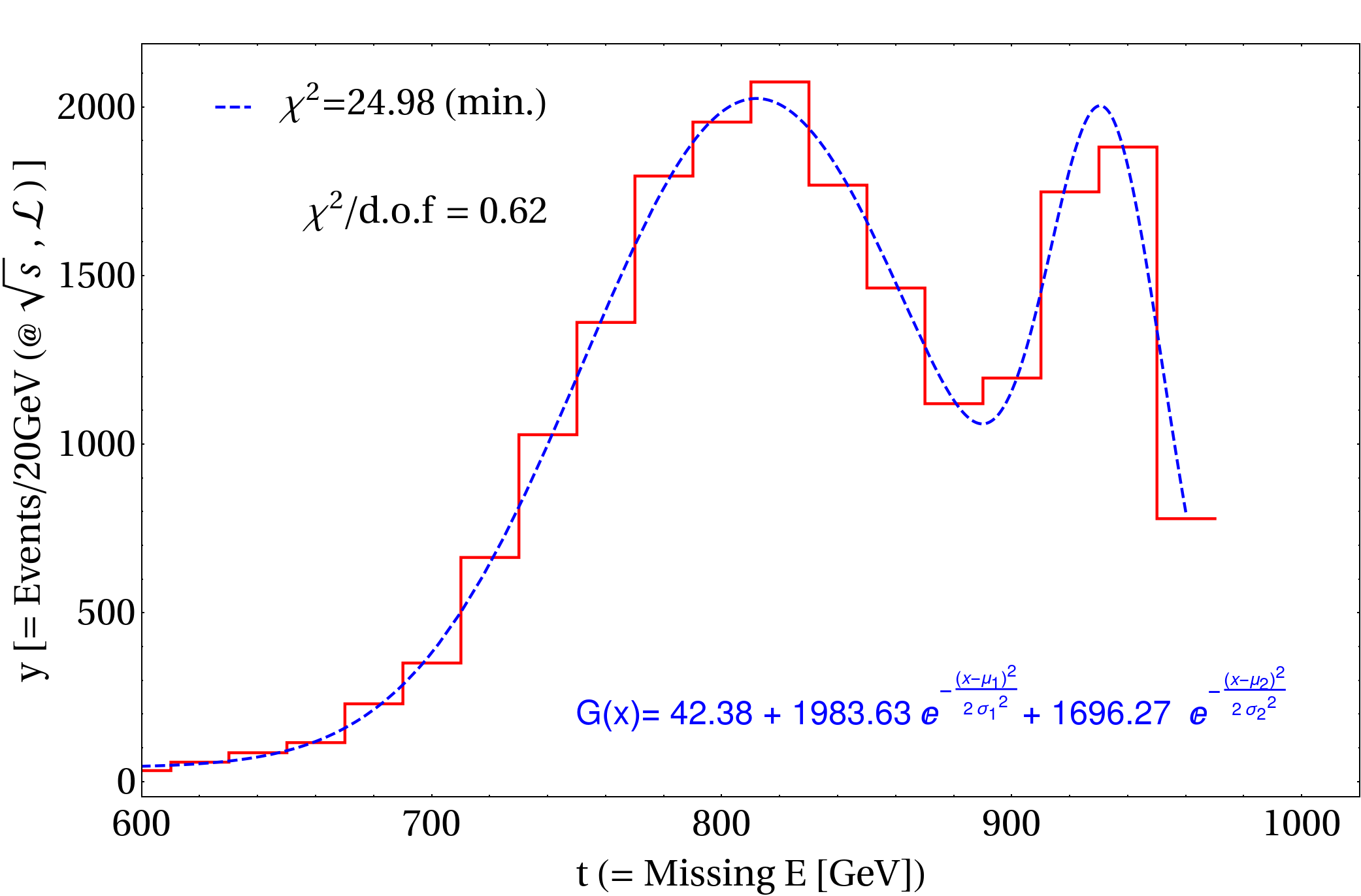
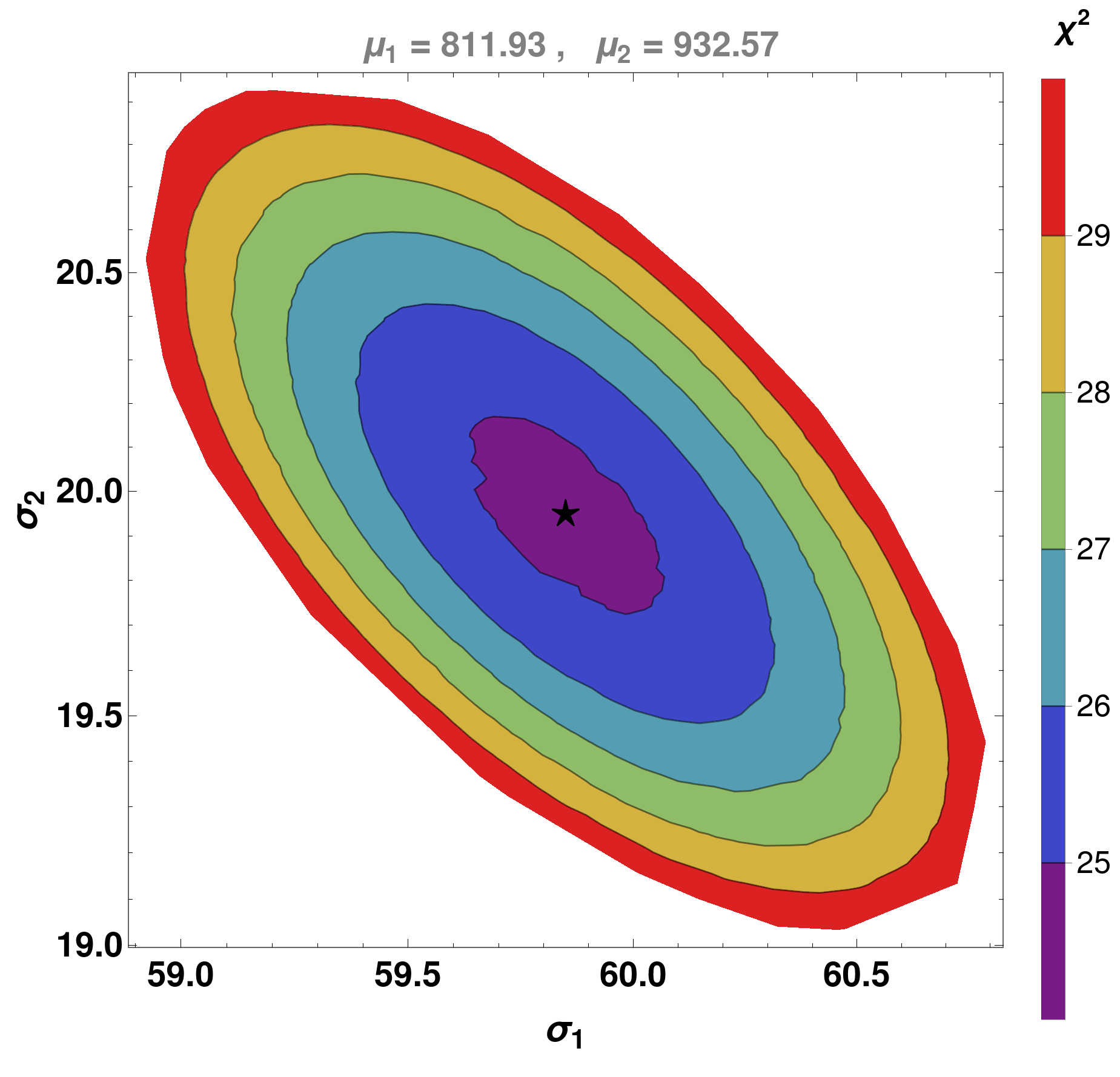
Figure 34: [Top Left] $\chi^{2}$ defined by Eq. 45 shown in different colored regions in the plane of $\sigma_{1}-\sigma_{2}$ for the random variation of the parameters of the two peak Gaussian function $G$: $\{\mu_{1}:\{810.2-813.4\},\sigma_{1}:\{58-62\};\mu_{2}:\{931.7-933.7\},\sigma_{2}:\{18-22\}\}$. [Top Right] The best fit two peak Gaussian function with minimum $\chi^{2}$ shown by blue dotted line, confronted with histogram data in solid red. [Bottom] The variation of $\chi^{2}$ is again shown in the plane of $\sigma_{1}-\sigma_{2}$ keeping $\mu_{1}=811.93$ and $\mu_{2}=932.57$ fixed. The $\star$ sign corresponds to the best fit parameters of the Gaussian function $G$, which also marks minimum $\chi^{2}$.

Consider that we have generated the histogram data by event simulation as,

$$\mathcal{H}=\{\{x_{H}^{1},y_{H}^{1}\},\{x_{H}^{2},y_{H}^{2}\},....,\{x_{H}^{n},y_{H}^{n}\}\}\,;$$ (43)

where $x_{H}\equiv\not{E},~{}y_{H}\equiv\frac{d\sigma}{d\not{E}}$ and $n$ refers to number of data points. We want to fit a two peak Gaussian function to this data as,

$$G(\mu_{1},\sigma_{1};\mu_{2},\sigma_{2}) = A_{1}~{}e^{-\frac{(x-\mu_{1})^{2}}{2\sigma_{1}^{2}}}+A_{2}~{}e^{-\frac{(x-\mu_{2})^{2}}{2\sigma_{2}^{2}}}+\cal{B}~{}.$$ (44)

Our goal is then to find out $\{\mu_{1},\sigma_{1}\}$ of the first peak and $\{\mu_{2},\sigma_{2}\}$ of the second peak of the above Gaussian function $G$ that best fit the histogram data $\mathcal{H}$. In order to do that we define $\chi^{2}$ function as:

$$\chi^{2}(\mu_{1},\sigma_{1};\mu_{2},\sigma_{2})=\sum_{i=1}^{n}{\frac{\Big{(}G(\mu_{1},\sigma_{1};\mu_{2},\sigma_{2})[x_{H}^{i}]-y_{H}^{i}\Big{)}^{2}}{y_{H}^{i}}}~{}~{}.$$ (45)

The best fit function $G$ can be estimated by minimizing $\chi^{2}$; i.e. vary $(\mu_{1},\sigma_{1},\mu_{2},\sigma_{2})$, calculate $\chi^{2}$ using Eqn. 45, and choose the one that has minimum $\chi^{2}$. Note here that $A_{1},~{}A_{2}$ and $\cal{B}$ of the function $G$ are automatically decided from the fitting (so the area under the curve remains the same) for a fixed set of $(\mu_{1},\sigma_{1},\mu_{2},\sigma_{2})$. For example, we randomly vary: $(\mu_{1}:\{810.2-813.4\},\sigma_{1}:\{58-62\},\mu_{2}:\{931.7-933.7\},\sigma_{2}:\{18-22\})$ for a particular data set, as shown in the top left panel of Fig. 34 in the plane of $\sigma_{1}-\sigma_{2}$. The different color patches here correspond to different $\chi^{2}$ ranges. The minimum $\chi^{2}$ value, $\chi_{\rm min}^{2}=24.98$ provides the best fit parameters of $G$, marked by $\star$, where the values of the parameters turn out to be: $\{\mu_{1}^{0},\sigma_{1}^{0};\mu_{2}^{0},\sigma_{2}^{0}\}=\{811.93,59.85;932.57,19.95\}$. We further use this best fit Gaussian function, $G(\mu_{1}^{0},\sigma_{1}^{0};\mu_{2}^{0},\sigma_{2}^{0})$ and draw the distribution by blue dotted line on top of the Histogram data (red thick line) as shown in the right top panel of Fig. 34. The particular histogram data uses the simulated events for BP1 $\{m_{\rm DM_{1}},m_{\rm DM_{2}},\Delta m_{1},\Delta m_{2}\}=\{100,60.5,10,370\}$ GeV. This exercise has been repeated for all the cases analysed in the text. We also estimate the $\chi^{2}/{\rm d.o.f}$ of the Gaussian fit where d.o.f refers to the number of histogram data sets. In this particular example, we find $\chi^{2}/{\rm d.o.f}=0.62$. Note here that any value for $\chi^{2}/{\rm d.o.f}<1$ is considered pretty accurate. In the bottom panel of Fig. 34, we show the variation of $\chi^{2}$ in the plane of $\sigma_{1}-\sigma_{2}$ keeping $\mu_{1}=811.93$ and $\mu_{2}=932.57$ fixed. As expected, it shows a set of parabola having constant $\chi^{2}$ ranges.

Appendix E Effect of polarisation in distinguishing two peaks

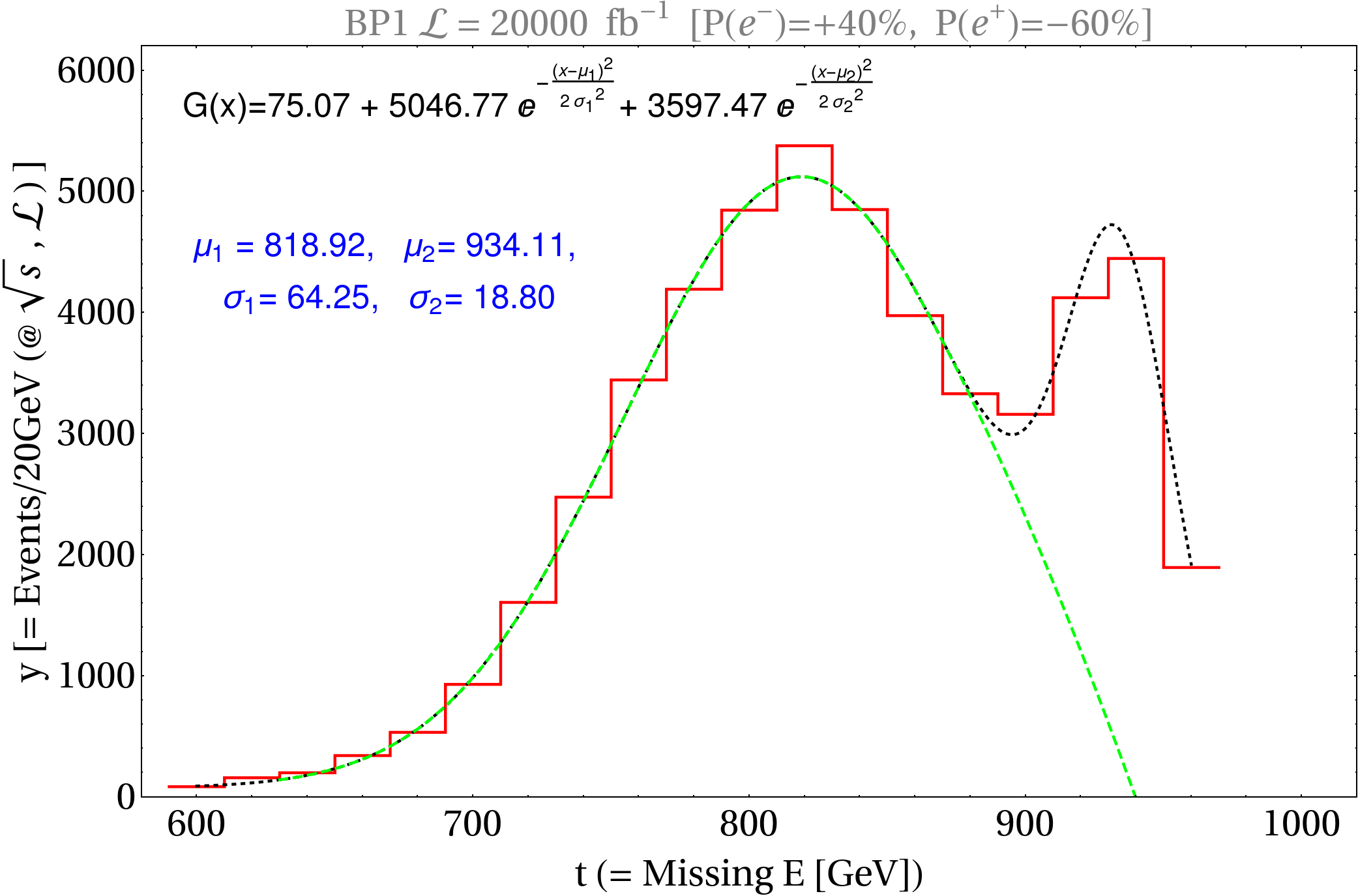
(a)

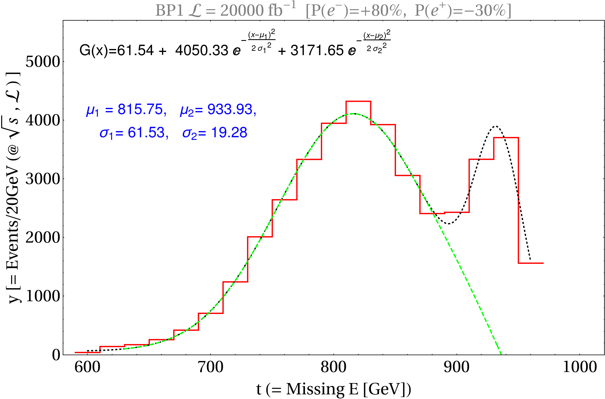
(b)

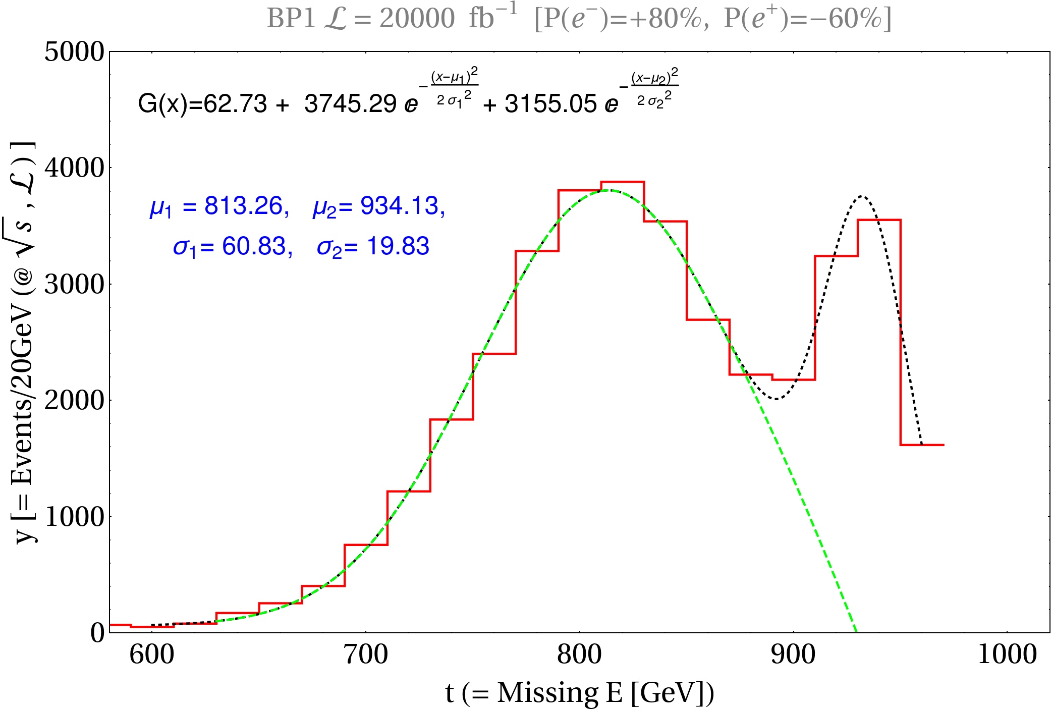
(c)

Figure 35: $\not{E}$ distribution for BP1 together with SM background and Gaussian fit for different beam polarizations: (a) $P1^{{}^{\prime}}\equiv\{P_{e^{-}}:+0.4,P_{e^{+}}:-0.6\};~{}(b)~{}P3\equiv\{P_{e^{-}}:+0.8,P_{e^{+}}:-0.3\}$ and (c) $P3^{{}^{\prime}}\equiv\{P_{e^{-}}:+0.8,P_{e^{+}}:-0.6\}$.

We study the effect of polarization in two-peak identification in this section. In Fig. 35, we show the Gaussian fit of the $\not{E}$ distribution for BP1 with right polarised electron and left polarised positron of three different degrees: $P1^{{}^{\prime}}\equiv\{P_{e^{-}}:+0.4,P_{e^{+}}:-0.6\};~{}P3\equiv\{P_{e^{-}}:+0.8,P_{e^{+}}:-0.3\}$ and $P3^{{}^{\prime}}\equiv\{P_{e^{-}}:0.8,P_{e^{+}}:-0.6\}$. Following previous discussion, it is clear that SM background is largest for $P1^{{}^{\prime}}$ and smallest for $P3^{{}^{\prime}}$. Consequently relative size of the second peak is highest for $P3^{{}^{\prime}}$ and smallest for $P1^{{}^{\prime}}$. The luminosity is chosen high just to capture the effect of polarization.

We check conditions C1-C4 for all the aforementioned choices of polarisation for BP1. In Fig. 36(a), we show the dependence of $R_{C1}$ as function of $\mathcal{L}$, for $n=1.2,1.5$. Here we see that $R_{C1}$ is largest for $P1^{{}^{\prime}}$, simply because more number of events under the first peak due to background contamination. We check C2 next in Fig. 36(b), where again $P1^{{}^{\prime}}$ does best and larger $k$ is required to achieve $R_{C2}$ $\raisebox{-3.69899pt}{~{}\shortstack{$>$ \\ [-0.07cm] $\sim$}}~{}2$ at lower luminosities. The condition C3 is checked in Fig. 36 (c). Again, $R_{C3}$ is larger for $P1^{{}^{\prime}}$ and lowest in $P3^{{}^{\prime}}$ as it captures the height difference between the peaks. Fig. 36(d) shows $R_{C4}$ as a function $\mathcal{L}$; here, $P3^{{}^{\prime}}$ is maximum. We conclude that polarisation, although necessary for reducing SM background, doesn’t alter the distinguishability of the two peaks significantly when varied within a range as $P1^{{}^{\prime}}-P3^{{}^{\prime}}$.

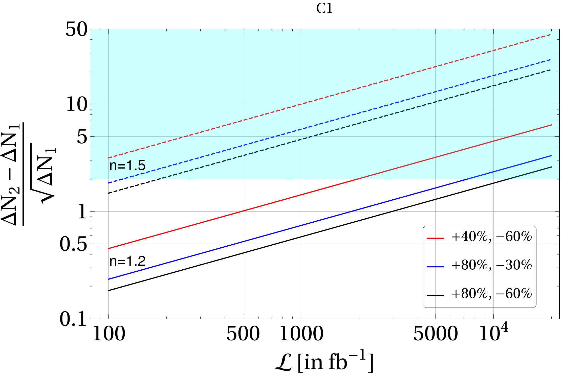
(a)

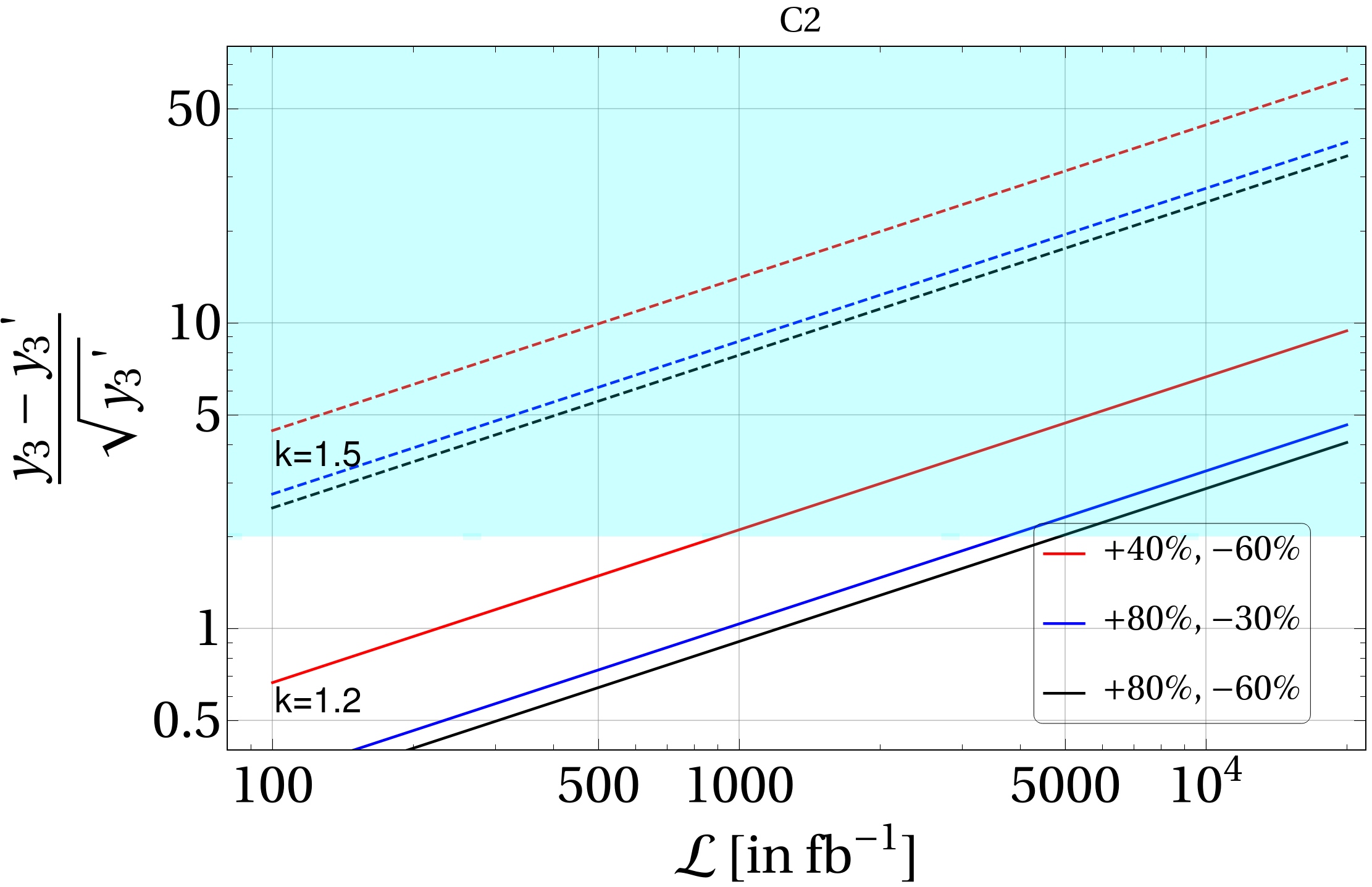
(b)

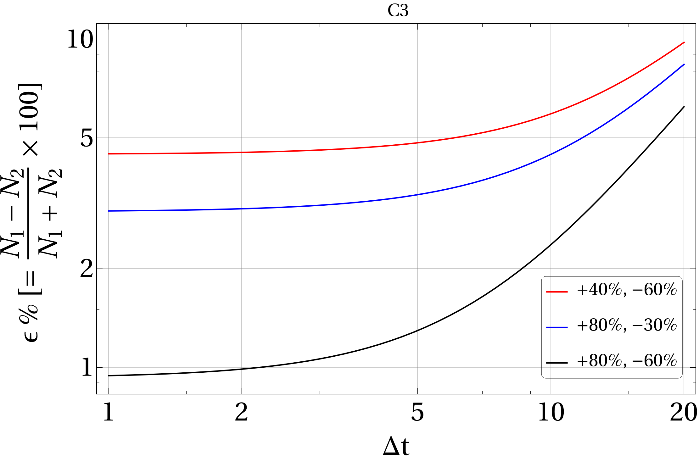
(c)

(d)

Figure 36: Condition C1-C4 for BP1 for various polarization configurations, $P1^{{}^{\prime}}\equiv\{P_{e^{-}}:+0.4,P_{e^{+}}:-0.6\};~{}P3\equiv\{P_{e^{-}}:+0.8,P_{e^{+}}:-0.3\}$ and $P3^{{}^{\prime}}\equiv\{P_{e^{-}}:0.8,P_{e^{+}}:-0.6\}$. (a) $R_{C1}$ as a function of $\mathcal{L}$ for different $n$ values (sky blue shaded region marks $R_{C1}\geq 2$); (b) Same as (a) but for $R_{C2}$; (c) $R_{C3}$ as function of $\Delta t$ and (d) Same as (a), but for $R_{C4}$.

References

- (1) V. C. Rubin and W. K. Ford, Jr., Rotation of the Andromeda Nebula from a Spectroscopic Survey of Emission Regions, Astrophys. J. 159 (1970) 379–403.
- (2) F. Zwicky, On the Masses of Nebulae and of Clusters of Nebulae, Astrophys. J. 86 (1937) 217–246.
- (3) E. Hayashi and S. D. M. White, How Rare is the Bullet Cluster?, Mon. Not. Roy. Astron. Soc. 370 (2006) L38–L41, [astro-ph/0604443].
- (4) W. Hu and S. Dodelson, Cosmic microwave background anisotropies, Ann. Rev. Astron. Astrophys. 40 (2002) 171–216, [astro-ph/0110414].
- (5) WMAP collaboration, G. Hinshaw et al., Nine-Year Wilkinson Microwave Anisotropy Probe (WMAP) Observations: Cosmological Parameter Results, Astrophys. J. Suppl. 208 (2013) 19, [1212.5226].
- (6) WMAP collaboration, D. N. Spergel et al., Wilkinson Microwave Anisotropy Probe (WMAP) three year results: implications for cosmology, Astrophys. J. Suppl. 170 (2007) 377, [astro-ph/0603449].
- (7) Planck collaboration, N. Aghanim et al., Planck 2018 results. VI. Cosmological parameters, Astron. Astrophys. 641 (2020) A6, [1807.06209].
- (8) G. Bertone, D. Hooper and J. Silk, Particle dark matter: Evidence, candidates and constraints, Phys. Rept. 405 (2005) 279–390, [hep-ph/0404175].
- (9) L. Roszkowski, E. M. Sessolo and S. Trojanowski, WIMP dark matter candidates and searches—current status and future prospects, Rept. Prog. Phys. 81 (2018) 066201, [1707.06277].
- (10) E. W. Kolb and M. S. Turner, The Early Universe, Front. Phys. 69 (1990) 1–547.
- (11) L. J. Hall, K. Jedamzik, J. March-Russell and S. M. West, Freeze-In Production of FIMP Dark Matter, JHEP 03 (2010) 080, [0911.1120].
- (12) M. Aoki, M. Duerr, J. Kubo and H. Takano, Multi-Component Dark Matter Systems and Their Observation Prospects, Phys. Rev. D86 (2012) 076015, [1207.3318].
- (13) Z.-P. Liu, Y.-L. Wu and Y.-F. Zhou, Enhancement of dark matter relic density from the late time dark matter conversions, Eur. Phys. J. C71 (2011) 1749, [1101.4148].
- (14) Q.-H. Cao, E. Ma, J. Wudka and C. P. Yuan, Multipartite dark matter, 0711.3881.
- (15) S. Bhattacharya, A. Drozd, B. Grzadkowski and J. Wudka, Two-Component Dark Matter, JHEP 10 (2013) 158, [1309.2986].
- (16) S. Esch, M. Klasen and C. E. Yaguna, A minimal model for two-component dark matter, JHEP 09 (2014) 108, [1406.0617].
- (17) A. Karam and K. Tamvakis, Dark Matter from a Classically Scale-Invariant , Phys. Rev. D94 (2016) 055004, [1607.01001].
- (18) A. Ahmed, M. Duch, B. Grzadkowski and M. Iglicki, Multi-Component Dark Matter: the vector and fermion case, Eur. Phys. J. C78 (2018) 905, [1710.01853].
- (19) A. Poulin and S. Godfrey, Multicomponent dark matter from a hidden gauged SU(3), Phys. Rev. D99 (2019) 076008, [1808.04901].
- (20) M. Aoki and T. Toma, Boosted Self-interacting Dark Matter in a Multi-component Dark Matter Model, JCAP 1810 (2018) 020, [1806.09154].
- (21) S. Yaser Ayazi and A. Mohamadnejad, Scale-Invariant Two Component Dark Matter, Eur. Phys. J. C79 (2019) 140, [1808.08706].
- (22) M. Aoki, D. Kaneko and J. Kubo, Multicomponent Dark Matter in Radiative Seesaw Models, Front.in Phys. 5 (2017) 53, [1711.03765].
- (23) A. Biswas, D. Majumdar, A. Sil and P. Bhattacharjee, Two Component Dark Matter : A Possible Explanation of 130 GeV Ray Line from the Galactic Centre, JCAP 1312 (2013) 049, [1301.3668].
- (24) S. Bhattacharya, P. Poulose and P. Ghosh, Multipartite Interacting Scalar Dark Matter in the light of updated LUX data, JCAP 1704 (2017) 043, [1607.08461].
- (25) S. Bhattacharya, P. Ghosh, T. N. Maity and T. S. Ray, Mitigating Direct Detection Bounds in Non-minimal Higgs Portal Scalar Dark Matter Models, JHEP 10 (2017) 088, [1706.04699].
- (26) B. Barman, S. Bhattacharya and M. Zakeri, Multipartite Dark Matter in extension of Standard Model and signatures at the LHC, JCAP 1809 (2018) 023, [1806.01129].
- (27) S. Bhattacharya, P. Ghosh and N. Sahu, Multipartite Dark Matter with Scalars, Fermions and signatures at LHC, JHEP 02 (2019) 059, [1809.07474].
- (28) S. Bhattacharya, P. Ghosh, A. K. Saha and A. Sil, Two component dark matter with inert Higgs doublet: neutrino mass, high scale validity and collider searches, JHEP 03 (2020) 090, [1905.12583].
- (29) D. Borah, R. Roshan and A. Sil, Minimal Two-component Scalar Doublet Dark Matter with Radiative Neutrino Mass, 1904.04837.
- (30) S. Chakraborti and P. Poulose, Interplay of Scalar and Fermionic Components in a Multi-component Dark Matter Scenario, 1808.01979.
- (31) S. Chakraborti, A. Dutta Banik and R. Islam, Probing Multicomponent Extension of Inert Doublet Model with a Vector Dark Matter, 1810.05595.
- (32) S. Bhattacharya, A. K. Saha, A. Sil and J. Wudka, Dark Matter as a remnant of SQCD Inflation, JHEP 10 (2018) 124, [1805.03621].
- (33) C. E. Yaguna and O. Zapata, Fermion and scalar two-component dark matter from a symmetry, 2112.07020.
- (34) G. Belanger, A. Mjallal and A. Pukhov, Two dark matter candidates: The case of inert doublet and singlet scalars, Phys. Rev. D 105 (2022) 035018, [2108.08061].
- (35) D. Van Loi, N. M. Duc and P. V. Dong, Dequantization of electric charge: Probing scenarios of cosmological multi-component dark matter, 2106.12278.
- (36) C. E. Yaguna and O. Zapata, Two-component scalar dark matter in Z2n scenarios, JHEP 10 (2021) 185, [2106.11889].
- (37) B. Díaz Sáez, K. Möhling and D. Stöckinger, Two real scalar WIMP model in the assisted freeze-out scenario, JCAP 10 (2021) 027, [2103.17064].
- (38) N. Chakrabarty, R. Roshan and A. Sil, Two Component Doublet-Triplet Scalar Dark Matter stabilising the Electroweak vacuum, 2102.06032.
- (39) C. H. Nam, D. Van Loi, L. X. Thuy and P. Van Dong, Multicomponent dark matter in noncommutative gauge theory, JHEP 12 (2020) 029, [2006.00845].
- (40) A. Betancur, G. Palacio and A. Rivera, Inert doublet as multicomponent dark matter, Nucl. Phys. B 962 (2021) 115276, [2002.02036].
- (41) D. Nanda and D. Borah, Connecting Light Dirac Neutrinos to a Multi-component Dark Matter Scenario in Gauged Model, Eur. Phys. J. C 80 (2020) 557, [1911.04703].
- (42) S. Bhattacharya, N. Chakrabarty, R. Roshan and A. Sil, Multicomponent dark matter in extended : neutrino mass and high scale validity, JCAP 04 (2020) 013, [1910.00612].
- (43) F. Elahi and S. Khatibi, Multi-Component Dark Matter in a Non-Abelian Dark Sector, Phys. Rev. D 100 (2019) 015019, [1902.04384].
- (44) J. Herrero-Garcia, A. Scaffidi, M. White and A. G. Williams, Time-dependent rate of multicomponent dark matter: Reproducing the DAMA/LIBRA phase-2 results, Phys. Rev. D 98 (2018) 123007, [1804.08437].
- (45) A. Das, S. Gola, S. Mandal and N. Sinha, Two-component scalar and fermionic dark matter candidates in a generic U model, 2202.01443.
- (46) S. Bhattacharya, S. Chakraborti and D. Pradhan, Electroweak Symmetry Breaking and WIMP-FIMP Dark Matter, 2110.06985.
- (47) A. Dutta Banik, M. Pandey, D. Majumdar and A. Biswas, Two component WIMP–FImP dark matter model with singlet fermion, scalar and pseudo scalar, Eur. Phys. J. C 77 (2017) 657, [1612.08621].
- (48) S.-M. Choi, J. Kim, P. Ko and J. Li, A multi-component SIMP model with , JHEP 09 (2021) 028, [2103.05956].
- (49) XENON collaboration, E. Aprile et al., Dark Matter Search Results from a One Ton-Year Exposure of XENON1T, Phys. Rev. Lett. 121 (2018) 111302, [1805.12562].
- (50) PandaX-4T collaboration, Y. Meng et al., Dark Matter Search Results from the PandaX-4T Commissioning Run, Phys. Rev. Lett. 127 (2021) 261802, [2107.13438].
- (51) J. Herrero-Garcia, A. Scaffidi, M. White and A. G. Williams, On the direct detection of multi-component dark matter: sensitivity studies and parameter estimation, JCAP 1711 (2017) 021, [1709.01945].
- (52) J. Herrero-Garcia, A. Scaffidi, M. White and A. G. Williams, On the direct detection of multi-component dark matter: implications of the relic abundance, JCAP 1901 (2019) 008, [1809.06881].
- (53) J. Hernandez-Sanchez, V. Keus, S. Moretti, D. Rojas-Ciofalo and D. Sokolowska, Complementary Probes of Two-component Dark Matter, 2012.11621.
- (54) P. Konar, K. Kong, K. T. Matchev and M. Park, Dark Matter Particle Spectroscopy at the LHC: Generalizing M(T2) to Asymmetric Event Topologies, JHEP 04 (2010) 086, [0911.4126].
- (55) K. Agashe, D. Kim, D. G. E. Walker and L. Zhu, Using to Distinguish Dark Matter Stabilization Symmetries, Phys. Rev. D 84 (2011) 055020, [1012.4460].
- (56) G. F. Giudice, B. Gripaios and R. Mahbubani, Counting dark matter particles in LHC events, Phys. Rev. D 85 (2012) 075019, [1108.1800].
- (57) G. Bélanger et al., LHC-friendly minimal freeze-in models, JHEP 02 (2019) 186, [1811.05478].
- (58) J. Alimena et al., Searching for long-lived particles beyond the Standard Model at the Large Hadron Collider, J. Phys. G 47 (2020) 090501, [1903.04497].
- (59) S. Banerjee, G. Bélanger, A. Ghosh and B. Mukhopadhyaya, Long-lived stau, sneutrino dark matter and right-slepton spectrum, JHEP 09 (2018) 143, [1806.04488].
- (60) S. P. Liew, M. Papucci, A. Vichi and K. M. Zurek, Mono-X Versus Direct Searches: Simplified Models for Dark Matter at the LHC, JHEP 06 (2017) 082, [1612.00219].
- (61) F. Kahlhoefer, Review of LHC Dark Matter Searches, Int. J. Mod. Phys. A 32 (2017) 1730006, [1702.02430].
- (62) A. Boveia and C. Doglioni, Dark Matter Searches at Colliders, Ann. Rev. Nucl. Part. Sci. 68 (2018) 429–459, [1810.12238].
- (63) D. Abercrombie et al., Dark Matter benchmark models for early LHC Run-2 Searches: Report of the ATLAS/CMS Dark Matter Forum, Phys. Dark Univ. 27 (2020) 100371, [1507.00966].
- (64) J. Abdallah et al., Simplified Models for Dark Matter Searches at the LHC, Phys. Dark Univ. 9-10 (2015) 8–23, [1506.03116].
- (65) B. Barman, S. Bhattacharya, S. Girmohanta and S. Jahedi, Catch ’em all: Effective Leptophilic WIMPs at the Collider, 2109.10936.
- (66) E. M. Dolle and S. Su, The Inert Dark Matter, Phys. Rev. D 80 (2009) 055012, [0906.1609].
- (67) M. Dutta, S. Bhattacharya, P. Ghosh and N. Sahu, Singlet-Doublet Majorana Dark Matter and Neutrino Mass in a minimal Type-I Seesaw Scenario, JCAP 03 (2021) 008, [2009.00885].
- (68) K. Kannike, Vacuum Stability Conditions From Copositivity Criteria, Eur. Phys. J. C72 (2012) 2093, [1205.3781].
- (69) J. Chakrabortty, P. Konar and T. Mondal, Copositive Criteria and Boundedness of the Scalar Potential, Phys. Rev. D89 (2014) 095008, [1311.5666].
- (70) Searches for supersymmetric particles in e + e- collisions up to 208 gev and interpretation of the results within the mssm, The European Physical Journal C 31 (Dec, 2003) 421–479.
- (71) A. Pierce and J. Thaler, Natural Dark Matter from an Unnatural Higgs Boson and New Colored Particles at the TeV Scale, JHEP 08 (2007) 026, [hep-ph/0703056].
- (72) C. Degrande, C. Duhr, B. Fuks, D. Grellscheid, O. Mattelaer and T. Reiter, UFO - The Universal FeynRules Output, Comput. Phys. Commun. 183 (2012) 1201–1214, [1108.2040].
- (73) G. Bélanger, F. Boudjema, A. Goudelis, A. Pukhov and B. Zaldivar, micrOMEGAs5.0 : Freeze-in, Comput. Phys. Commun. 231 (2018) 173–186, [1801.03509].
- (74) MAGIC, Fermi-LAT collaboration, M. L. Ahnen et al., Limits to Dark Matter Annihilation Cross-Section from a Combined Analysis of MAGIC and Fermi-LAT Observations of Dwarf Satellite Galaxies, JCAP 02 (2016) 039, [1601.06590].
- (75) Fermi-LAT collaboration, M. Ackermann et al., Searching for Dark Matter Annihilation from Milky Way Dwarf Spheroidal Galaxies with Six Years of Fermi Large Area Telescope Data, Phys. Rev. Lett. 115 (2015) 231301, [1503.02641].
- (76) The International Linear Collider Technical Design Report - Volume 3.II: Accelerator Baseline Design, 1306.6328.
- (77) P. Bambade et al., The International Linear Collider: A Global Project, 1903.01629.
- (78) CLICdp, ILD concept group collaboration, A. F. Zarnecki, On the physics potential of ILC and CLIC, PoS CORFU2019 (2020) 037, [2004.14628].
- (79) J. Alwall, R. Frederix, S. Frixione, V. Hirschi, F. Maltoni, O. Mattelaer et al., The automated computation of tree-level and next-to-leading order differential cross sections, and their matching to parton shower simulations, JHEP 07 (2014) 079, [1405.0301].
- (80) DELPHES 3 collaboration, J. de Favereau, C. Delaere, P. Demin, A. Giammanco, V. Lemaître, A. Mertens et al., DELPHES 3, A modular framework for fast simulation of a generic collider experiment, JHEP 02 (2014) 057, [1307.6346].
- (81) H. Abramowicz et al., The International Linear Collider Technical Design Report - Volume 4: Detectors, 1306.6329.
- (82) S. Bhattacharya, P. Ghosh, J. Lahiri and B. Mukhopadhyaya, Mono-X signal and two component dark matter: new distinction criteria, 2211.10749.