Activation Functions: Dive into an optimal activation function

Abstract

Activation functions have come up as one of the essential components of neural networks. The choice of adequate activation function can impact the accuracy of these methods. In this study, we experiment for finding an optimal activation function by defining it as a weighted sum of existing activation functions and then further optimizing these weights while training the network. The study uses three activation functions, ReLU, tanh, and sin, over three popular image datasets, MNIST, FashionMNIST, and KMNIST. We observe that the ReLU activation function can easily overlook other activation functions. Also, we see that initial layers prefer to have ReLU or LeakyReLU type of activation functions, but deeper layers tend to prefer more convergent activation functions.

Keywords Activation Functions  $\cdot$ Deep Learning  $\cdot$ Neural Networks

1 Introduction

Deep Learning is currently one of the most booming fields(Alzubaidi et al. (2021)). Deep Neural Networks have been a standard component for all sorts of research done in the domain. These methods have acquired a wide variety of success in transforming the modern world. The development of many standard architectures has shown the effectiveness of these methods for various classification(Sharma et al. (2018)) and segmentation(Minaee et al. (2020)) tasks.

Many models namely, AlexNet(Krizhevsky (2014)), VGG(Simonyan and Zisserman (2014)), ResNet(He et al. (2016)), SqueezeNet(Iandola et al. (2016)), DenseNet(Huang et al. (2018)), Inception (Szegedy et al. (2015)), GoogLeNet(Szegedy et al. (2014)), etc., have gained popularity in recent years. This study focuses on one of the critical components in all the standard architectures, i.e., Activation Functions. Before going deep into the activation function, we need to understand how a neural network works.

Lets consider a input $x_{i}$ such that we need to predict $y$ and estimate a function $f(x_{i})$ with some error $\epsilon$ such that:

$$y=f(x_{i})+\epsilon$$ (1)

The simplest way we can find predicted value $\hat{y}$ is by writing $\hat{y}=w_{i}*x_{i}+b$, where $w_{i}$ stands for weight and $b$ stands for bais. now lets consider $X$ be a set of input features $[x_{1}~{}x_{2}.....~{}x_{n}]^{T}$ of shape $n\times 1$. In this scenario $\hat{y}$ can be written as:

$$\hat{y}=[w_{1}~{}w_{2}~{}w_{3}....~{}w_{n}][x_{1}~{}x_{2}.....~{}x_{n}]^{T}+[b]$$ (2)

Now, lets consider $y$ to be such that $[y_{1}~{}y_{2}.....~{}y_{m}]^{T}$ of shape $m\times 1$. In such a case weight matrix $W_{(1)}$ has to be defined of shape $n\times m$ and bias $B_{(1)}$ is defined of shape $m\times 1$. Therefore we can write the regression equation as:

$$\hat{y}=W_{(1)}^{T}X+B_{(1)}$$ (3)

Now, to model at a higher level we can further multiply another matrix $W_{(2)}$ with shape $n1\times m$ and bias $B_{(2)}$ of shape $m\times 1$. Also we modify weight matrix $W_{(1)}$ has to be defined of shape $n\times n1$ and bias $B_{(1)}$ is defined of shape $n1\times 1$. Hence, we can find $\hat{y}$ as:

$$\hat{y}=W_{(2)}^{T}(W_{(1)}^{T}X+B_{(1)})+B_{(2)}$$ (4)

But just using additional matrix $W_{(2)}$, would not solve the problem of modelling difficult functions. Hence there is a need of a function that can add non-linearity to the model. Hence activation function $\mathcal{A}_{1}(.)$ and $\mathcal{A}_{2}(.)$ are required. Hence we can write final equation 5 as:

$$\hat{y}=\mathcal{A}_{2}(W_{(2)}^{T}\mathcal{A}_{1}(W_{(1)}^{T}X+B_{(1)})+B_{(2)})$$ (5)

The choice of activation function can actually be sometime quite tricky. There are wide variety of popular activation function namely, ReLU, Sigmoid, Tanh, GeLU, GLU(Hendrycks and Gimpel (2020)), Swish(Ramachandran et al. (2017)), Softplus, Mish (Misra (2020)), PRelU(He et al. (2015)), SeLU(Klambauer et al. (2017)), Maxout(Goodfellow et al. (2013)), ReLU6(Howard et al. (2017)), HardSwish (Howard et al. (2019)), ELU(Clevert et al. (2016)), Shifted Softplus(schütt2017schnet), SiLU(Elfwing et al. (2017)), CReLU(Shang et al. (2016)), modReLU(Arjovsky et al. (2016)), KAF(Scardapane et al. (2017)), TanhExp(Liu and Di (2020)) etc.

2 Experimental Setup

In this work we are looking for a possibility of a better activation function by expressing it as a weighted sum of multiple activation functions and then optimizing those weights for them to find the dominant activation function.

To start with we take 3 common machine learning datasets, MNIST(Lecun et al. (1998)), Fashion MNIST(Xiao et al. (2017)) and KMNIST(Clanuwat et al. (2018)). Further, we need to choose a network for experimentation. The model used consist of two convolutional layers followed by two fully connected layers. There are activation functions between the layers which is weighted in format. We take 3 functions as activation function, ReLU($f_{1}$), Tanh($f_{2}$) and sin($f_{3}$) as given below:

$$f_{1}(x)=ReLU(x)=max(o,x)$$ (6)

$$f_{2}(x)=tanh(x)=\frac{exp(x)-exp(-x)}{exp(x)+exp(-x)}$$ (7)

$$f_{3}(x)=Sin(x)$$ (8)

Now further we define weights $w_{1}$, $w_{2}$, and $w_{3}$ such that $w_{1},w_{2},w_{3}\geq 0$. Using these we find parameters as $P_{1}$, $P_{2}$ and $P_{3}$ such that:

$$P_{i}=\frac{w_{i}}{\Sigma w_{i}},~{}for~{}i=1,2,3$$ (9)

Finally we define activation function $A(.)$ as:

$$A(x)=P_{1}f_{1}(x)+P_{2}f_{2}(x)+P_{3}f_{3}(x)$$ (10)

In the above equation $0\leq P_{i}\leq 1$ always. For each layer we define a set of unique parameters $w_{1},w_{2},w_{3}$ for each activation function.

For training this network we adopt a unique strategy using Adam optimizer and adoption of three cycle of training. For the first cycle we start with freezing the weights $w_{1},w_{2},w_{3}$ and training the parameters of all other layers with a learning rate of $1e-3$ for 10 epochs. Then further freezing the parameters of convolutional and fully connected layers and allowing training of only $w_{1},w_{2},w_{3}$ with a learning rate of $1e-2$ for 10 epochs. At last, we again freeze the weights $w_{1},w_{2},w_{3}$ and train the parameters of all other layers with a learning rate of $1e-3$ for 10 epochs. We look into the final activation functions and weights for analysis.

3 Results and Discussion

In this section we discuss the results from various experiments on the three datasets. Table 1 shows the results obtained for all three datasets for all 3 layers of activation function for parameters $P_{1}$, $P_{2}$, and $P_{3}$. The Figure 1 shows the activation functions for the corresponding layers for a range of value given $-3\leq x\leq 3$.

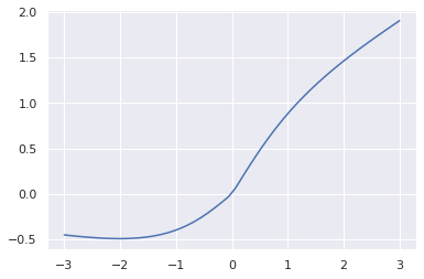
(a)

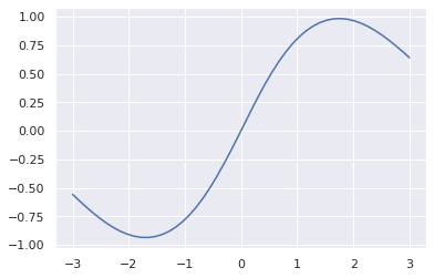
(b)

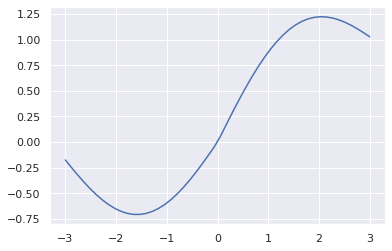
(c)

(d)

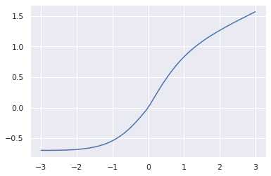
(e)

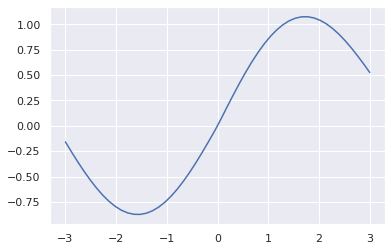
(f)

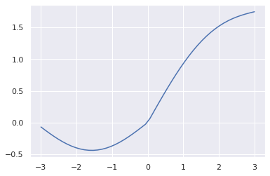
(g)

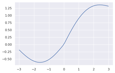
(h)

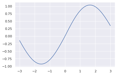
(i)

Figure 1: Activation Function for MNIST((a) Layer 1, (b) Layer 2, (c) Layer 3)), Fashion MNIST ((d) Layer 1, (e) Layer 2, (f) Layer 3))and KMNIST((g) Layer 1, (h) Layer 2, (i) Layer 3))

We refer $A_{1}$ to be activation function of first layer of the network and write the same as for MNIST, Fashion MNIST and KMNIST:

$$A_{1}=0.4848f_{1}+0.4437f_{2}+0.0715f_{3}~{}for~{}MNIST$$ (11)

$$A_{1}=0.5178f_{1}+0.1470f_{2}+0.3352f_{3}~{}for~{}FashionMNIST$$ (12)

$$A_{1}=0.5590f_{1}+0.0101f_{2}+0.4309f_{3}~{}for~{}KMNIST$$ (13)

Table 1: Weights $P_{1},P_{2},P_{3}$ for various activation layters for various datasets

DATASETS	LAYERS	$P_{1}$	$P_{2}$	$P_{3}$
	LAYER 1	0.4848	0.4437	0.0715
MNIST	LAYER 2	0.0276	0.4923	0.48
	LAYER 3	0.284	0.0877	0.6283
	LAYER 1	0.5178	0.147	0.3352
FashionMNIST	LAYER 2	0.2907	0.7001	0.0091
	LAYER 3	0.1221	0.041	0.8369
	LAYER 1	0.559	0.0101	0.4309
KMNIST	LAYER 2	0.3754	0.1167	0.5079
	LAYER 3	0.0679	0.0156	0.9165

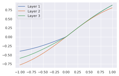
(a)

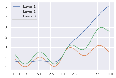
(b)

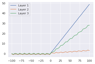
(c)

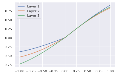
(d)

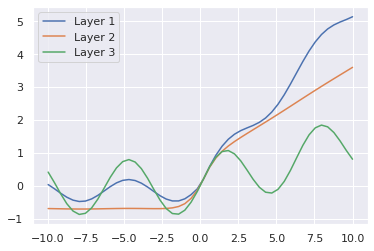
(e)

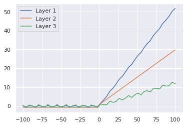
(f)

(g)

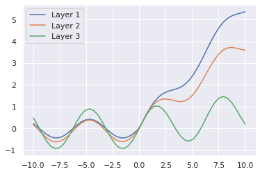
(h)

(i)

Figure 2: Activation Function for MNIST((a) $-1\leq x\leq 1$, (b) $-10\leq x\leq 10$, (c)$-100\leq x\leq 100$)), Fashion MNIST ((a) $-1\leq x\leq 1$, (b) $-10\leq x\leq 10$, (c)$-100\leq x\leq 100$))and KMNIST((a) $-1\leq x\leq 1$, (b) $-10\leq x\leq 10$, (c)$-100\leq x\leq 100$))

From the equation 11, 12 and 13 we can observe that first activation layer is more dominated by ReLU ($f_{1}$) activation function. This shows that for first layer of a network it would always be prefered to choose an activation function similar to ReLU activation function. When we further take a look into activation layers $A_{2}$ and $A_{3}$, we observe that the cofficient of ReLU activation function is smaller than that of other activation functions.

$$A_{2}=0.0276f_{1}+0.4923f_{2}+0.4800f_{3}~{}for~{}MNIST$$ (14)

$$A_{2}=0.2907f_{1}+0.7001f_{2}+0.0091f_{3}~{}for~{}FashionMNIST$$ (15)

$$A_{2}=0.3754f_{1}+0.1167f_{2}+0.5079f_{3}~{}for~{}KMNIST$$ (16)

$$A_{3}=0.2840f_{1}+0.0877f_{2}+0.6283f_{3}~{}for~{}MNIST$$ (17)

$$A_{3}=0.1221f_{1}+0.0410f_{2}+0.8369f_{3}~{}for~{}FashionMNIST$$ (18)

$$A_{3}=0.0679f_{1}+0.0156f_{2}+0.9165f_{3}~{}for~{}KMNIST$$ (19)

After we observe the activation function for individual layer we look for observing them in various ranges of input. When we take $-1\leq x\leq 1$ than we observe the plot in figure 2 (a), (d), and (e). We find that activation function can be approximately written as:

$$A=\begin{cases}h_{1}*x,&if~{}x\geq 0\\ h_{2}*x,&\text{otherwise}\end{cases}$$ (20)

In the above activation function $h_{1}$ and $h_{2}$ are arbitrary small constants. The above function can be transfered and written as LeakyReLU activation function by taking $h_{1}=1$ and $h_{2}$ be a small value. hence it can be written as:

$$A=max(h_{2}*x,x)=LeakyReLU(X)$$ (21)

If we take a broader look these approximations are good for activation function in initial layer of the network, but as we go deeper we observe that more convergent activation functions start becoming dominant. But, when $x$ starts to be larger we observe that ReLU can easily dominate other activation functions because of it larger value as shown in Figure 2 (c), (f), and (i).

4 Conclusion

This work shows an experimental study of utilizing a weighted linear combination of activation functions, looking for a better activation function needed by the model. We observe that the ReLU activation function is a powerful activation function that can overlook other activation functions when used in conjunction. We also follow that initial activation layers prefer a ReLU type or LeakyReLU activation function. We observe that networks prefer more convergent activation functions like tanh, sigmoid or sin for deeper layers. We can further explore the possibility of utilizing more activation functions and experimenting with more datasets. Additionally, it is possible to use multiplicative combinations of activation functions that would help us find better and more robust activation functions for neural networks.

References

- Alzubaidi et al. [2021] Laith Alzubaidi, Jinglan Zhang, Amjad J Humaidi, Ayad Al-Dujaili, Ye Duan, Omran Al-Shamma, J Santamaría, Mohammed A Fadhel, Muthana Al-Amidie, and Laith Farhan. Review of deep learning: Concepts, cnn architectures, challenges, applications, future directions. Journal of big Data, 8(1):1–74, 2021.
- Sharma et al. [2018] Neha Sharma, Vibhor Jain, and Anju Mishra. An analysis of convolutional neural networks for image classification. Procedia Computer Science, 132:377–384, 2018. ISSN 1877-0509. doi:https://doi.org/10.1016/j.procs.2018.05.198. URL https://www.sciencedirect.com/science/article/pii/S1877050918309335. International Conference on Computational Intelligence and Data Science.
- Minaee et al. [2020] Shervin Minaee, Yuri Boykov, Fatih Porikli, Antonio Plaza, Nasser Kehtarnavaz, and Demetri Terzopoulos. Image segmentation using deep learning: A survey. CoRR, abs/2001.05566, 2020. URL https://arxiv.org/abs/2001.05566.
- Krizhevsky [2014] Alex Krizhevsky. One weird trick for parallelizing convolutional neural networks. CoRR, abs/1404.5997, 2014. URL http://arxiv.org/abs/1404.5997.
- Simonyan and Zisserman [2014] Karen Simonyan and Andrew Zisserman. Very deep convolutional networks for large-scale image recognition. arXiv preprint arXiv:1409.1556, 2014.
- He et al. [2016] Kaiming He, Xiangyu Zhang, Shaoqing Ren, and Jian Sun. Deep residual learning for image recognition. In Proceedings of the IEEE conference on computer vision and pattern recognition, pages 770–778, 2016.
- Iandola et al. [2016] Forrest N Iandola, Song Han, Matthew W Moskewicz, Khalid Ashraf, William J Dally, and Kurt Keutzer. Squeezenet: Alexnet-level accuracy with 50x fewer parameters and< 0.5 mb model size. arXiv preprint arXiv:1602.07360, 2016.
- Huang et al. [2018] Gao Huang, Zhuang Liu, Laurens van der Maaten, and Kilian Q. Weinberger. Densely connected convolutional networks, 2018.
- Szegedy et al. [2015] Christian Szegedy, Vincent Vanhoucke, Sergey Ioffe, Jonathon Shlens, and Zbigniew Wojna. Rethinking the inception architecture for computer vision, 2015.
- Szegedy et al. [2014] Christian Szegedy, Wei Liu, Yangqing Jia, Pierre Sermanet, Scott Reed, Dragomir Anguelov, Dumitru Erhan, Vincent Vanhoucke, and Andrew Rabinovich. Going deeper with convolutions, 2014.
- Hendrycks and Gimpel [2020] Dan Hendrycks and Kevin Gimpel. Gaussian error linear units (gelus), 2020.
- Ramachandran et al. [2017] Prajit Ramachandran, Barret Zoph, and Quoc V. Le. Searching for activation functions, 2017.
- Misra [2020] Diganta Misra. Mish: A self regularized non-monotonic activation function, 2020.
- He et al. [2015] Kaiming He, Xiangyu Zhang, Shaoqing Ren, and Jian Sun. Delving deep into rectifiers: Surpassing human-level performance on imagenet classification, 2015.
- Klambauer et al. [2017] Günter Klambauer, Thomas Unterthiner, Andreas Mayr, and Sepp Hochreiter. Self-normalizing neural networks, 2017.
- Goodfellow et al. [2013] Ian J. Goodfellow, David Warde-Farley, Mehdi Mirza, Aaron Courville, and Yoshua Bengio. Maxout networks, 2013.
- Howard et al. [2017] Andrew G. Howard, Menglong Zhu, Bo Chen, Dmitry Kalenichenko, Weijun Wang, Tobias Weyand, Marco Andreetto, and Hartwig Adam. Mobilenets: Efficient convolutional neural networks for mobile vision applications, 2017.
- Howard et al. [2019] Andrew Howard, Mark Sandler, Grace Chu, Liang-Chieh Chen, Bo Chen, Mingxing Tan, Weijun Wang, Yukun Zhu, Ruoming Pang, Vijay Vasudevan, Quoc V. Le, and Hartwig Adam. Searching for mobilenetv3, 2019.
- Clevert et al. [2016] Djork-Arné Clevert, Thomas Unterthiner, and Sepp Hochreiter. Fast and accurate deep network learning by exponential linear units (elus), 2016.
- Elfwing et al. [2017] Stefan Elfwing, Eiji Uchibe, and Kenji Doya. Sigmoid-weighted linear units for neural network function approximation in reinforcement learning, 2017.
- Shang et al. [2016] Wenling Shang, Kihyuk Sohn, Diogo Almeida, and Honglak Lee. Understanding and improving convolutional neural networks via concatenated rectified linear units, 2016.
- Arjovsky et al. [2016] Martin Arjovsky, Amar Shah, and Yoshua Bengio. Unitary evolution recurrent neural networks, 2016.
- Scardapane et al. [2017] Simone Scardapane, Steven Van Vaerenbergh, Simone Totaro, and Aurelio Uncini. Kafnets: kernel-based non-parametric activation functions for neural networks, 2017.
- Liu and Di [2020] Xinyu Liu and Xiaoguang Di. Tanhexp: A smooth activation function with high convergence speed for lightweight neural networks, 2020.
- Lecun et al. [1998] Y. Lecun, L. Bottou, Y. Bengio, and P. Haffner. Gradient-based learning applied to document recognition. Proceedings of the IEEE, 86(11):2278–2324, 1998. doi:10.1109/5.726791.
- Xiao et al. [2017] Han Xiao, Kashif Rasul, and Roland Vollgraf. Fashion-mnist: a novel image dataset for benchmarking machine learning algorithms, 2017.
- Clanuwat et al. [2018] Tarin Clanuwat, Mikel Bober-Irizar, Asanobu Kitamoto, Alex Lamb, Kazuaki Yamamoto, and David Ha. Deep learning for classical japanese literature. CoRR, abs/1812.01718, 2018. URL http://arxiv.org/abs/1812.01718.