Robust Mediation Analysis: The R Package robmed

Andreas Alfons, Nufer Y. Ates, Patrick J.F. Groenen Robust Mediation Analysis: The R Package robmed Robust Mediation Analysis: The R Package robmed Mediation analysis is one of the most widely used statistical techniques in the social, behavioral, and medical sciences. Mediation models allow to study how an independent variable affects a dependent variable indirectly through one or more intervening variables, which are called mediators. The analysis is often carried out via a series of linear regressions, in which case the indirect effects can be computed as products of coefficients from those regressions. Statistical significance of the indirect effects is typically assessed via a bootstrap test based on ordinary least-squares estimates. However, this test is sensitive to outliers or other deviations from normality assumptions, which poses a serious threat to empirical testing of theory about mediation mechanisms. The R package robmed implements a robust procedure for mediation analysis based on the fast-and-robust bootstrap methodology for robust regression estimators, which yields reliable results even when the data deviate from the usual normality assumptions. Various other procedures for mediation analysis are included in package robmed as well. Moreover, robmed introduces a new formula interface that allows to specify mediation models with a single formula, and provides various plots for diagnostics or visual representation of the results. mediation analysis, robust statistics, bootstrap, R mediation analysis, robust statistics, bootstrap, R Andreas Alfons
Econometric Institute
Erasmus School of Economics
Erasmus University Rotterdam
PO Box 1738
3000DR Rotterdam, The Netherlands
E-mail:
URL: https://personal.eur.nl/alfons/

1 Introduction

In the social, behavioral, and medical sciences, mediation analysis is a popular statistical technique for studying how an independent variable affects a dependent variable indirectly through an intervening variable called a mediator. For instance, erreygers18 find that poor sleep quality in adolescents explains cyberbullying through anger, and gaudiano10 report that the believability of hallucinations after treatment for psychotic disorders mediates the relationship between the type of treatment and distress after treatment. Figure 1 shows a diagram of the mediation model in its simplest form, which is given by the equations

$$M =i_{1}+aX+e_{1},$$ (1)

$$Y =i_{2}+bM+cX+e_{2},$$ (2)

$$Y =i_{3}+c^{\prime}X+e_{3},$$ (3)

where $Y$ denotes the dependent variable, $X$ the independent variable, $M$ the hypothesized mediator, $i_{1}$, $i_{2}$, $i_{3}$, $a$, $b$, $c$, and $c^{\prime}$ are regression coefficients to be estimated, and $e_{1}$, $e_{2}$, and $e_{3}$ are random error terms. The coefficients $c$ and $c^{\prime}$ are called the direct effect and total effect, respectively, of $X$ on $Y$. The product of coefficients $ab$ is called the indirect effect of $X$ on $Y$ and constitutes the main parameter of interest in mediation analysis. Under the usual assumption of independent and normally distributed error terms $e_{1}$, $e_{2}$, and $e_{3}$, it holds that $c^{\prime}=ab+c$ (e.g., mackinnon95), and the same holds for the corresponding ordinary least-squares (OLS) estimates.

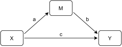
Figure 1: Diagram visualizing a simple mediation model.

The indirect effect $ab$ can be interpreted in the following way: a change of one unit in $X$ explains a change of $a$ units in $M$, which in turn explains a change of $ab$ units in $Y$. It is therefore an important question whether or not to standardize the variables in some way. If the scales of the variables differ by orders of magnitude, certain coefficients may dominate the relationship $c^{\prime}=ab+c$. However, variables used in mediation analysis often measure constructs that are aggregated from several rating-scale items (e.g., on a scale of 1–5). In such cases, a researcher may prefer not to standardize to keep the interpretation in terms of the original measurement scales. Similarly, a researcher may prefer not to standardize a binary $X$ variable to keep the interpretation in terms of a change from one group to the other. For a more detailed discussion on whether or not to use standardized coefficients in mediation analysis, we refer to hayes18.

Mediation analysis goes back to judd81 and baron86, however their stepwise approach has been superseded by approaches that focus on the indirect effect. sobel82 proposed a test for the indirect effect that assumes a normal distribution of the corresponding estimator, which is an unrealistic assumption for a product of coefficients. bollen90, shrout02, mackinnon04, and preacher04; preacher08 therefore advocate for a bootstrap test based on OLS regressions, which is the most frequently applied method for mediation analysis according to literature reviews of wood08 and alfons22a. More recently, several authors have emphasized that outliers or deviations from normality assumptions are detrimental to the reliability and validity of mediation analysis, and introduced more robust procedures. zu10 propose a bootstrap test after an initial data cleaning step, whereas yuan14 suggest a bootstrap test based on median regressions. alfons22a combine the robust MM-estimator of regression (yohai87) with the the fast-and-robust bootstrap (salibian02; salibian08), and demonstrate that this procedure outperforms the aforementioned approaches for a wide range of error distributions (with different levels of skewness and kurtosis) and outlier configurations.

Various software packages are available for mediation analysis. The macro INDIRECT (preacher04; preacher08) and its successor PROCESS (hayes18) for SPSS (SPSS) and SAS (SAS) implement the bootstrap test based on OLS regressions. For the statistical computing environment R (R), the general purpose packages psych (psych) and MBESS (MBESS) for statistical analysis in the behavioral sciences also provide functionality for a bootstrap test in mediation analysis. Package WRS2 (mair20) is a collection of robust statistical methods, which offers mediation analysis via the bootstrap test after data cleaning proposed by zu10. Other packages concentrate on mediation analysis or specific aspects thereof. Package mediation (tingley14) is focused on causal mediation analysis in a potential outcome framework, and package medflex (steen17) implements recent developments in mediation analysis embedded within the counterfactual framework. Bayesian multilevel mediation models can be estimated with package bmlm (bmlm), while package mma (mma) offers functionality for general multiple mediation analysis with continuous or binary/categorical variables. In addition, general purpose software for structural equation modeling such as Mplus (Mplus) or the R packages sem (sem) and lavaan (rosseel12) can be used for mediation analysis. The former also allows for maximum likelihood estimation with skew-normal, $t$, or skew-$t$ error distributions (asparouhov16).

Despite the growing number of R packages that address mediation analysis, there are no common interfaces or class structures. Instead, each package uses its own way of specifying mediation models and storing the results. Additionally, only package WRS2 contains some functionality for robust mediation analysis.

Package robmed (robmed) aims to address these issues. Its main functionality is the robust bootstrap procedure proposed in alfons22a, which is highly robust to outliers and other deviations from normality assumptions. Furthermore, robmed implements various other methods of estimating mediation models, as well as different tests for the indirect effects. All implemented methods share the same function interface and a clear class structure. In addition, robmed introduces a simple formula interface for specifying mediation models, and provides several plots for diagnostics or visualization of the results from mediation analysis.

Package robmed is available on CRAN (the Comprehensive R Archive Network, https://CRAN.R-project.org/) and can be installed from the R console with the following command: R> install.packages("robmed")

The rest of the paper is organized as follows. Section 2 discusses various extensions of the simple mediation model, as well as the implemented methodology for estimation and testing. Implementation details are provided in Section 3, while Section 4 illustrates the use of package robmed with code examples. The final Section LABEL:sec:summary concludes.

2 Methodology

We first provide overviews of the mediation models and estimation techniques supported by package robmed in Sections 2.1 and 2.2, respectively. Section 2.3 then gives technical details of the robust bootstrap procedure of alfons22a.

2.1 Extensions of the simple mediation model

The simple mediation model (1)–(3) can easily be extended in various ways, for instance with (i) multiple parallel mediators, (ii) multiple serial mediators, and (iii) multiple independent variables to be mediated. All those extensions may include additional control variables (covariates) as well.

2.1.1 Parallel multiple mediator model

In the parallel multiple mediator model, an independent variable $X$ is hypothesized to influence a dependent variable $Y$ through multiple mediators $M_{1},\dots,M_{k}$, while the mediator variables do not influence each other. A diagram of the model is displayed in Figure 2, and the corresponding regression equations are

$$M_{j} =i_{j}+a_{j}X+e_{j},\qquad j=1,\dots,k,$$ (4)

$$Y =i_{k+1}+b_{1}M_{1}+\dots+b_{k}M_{k}+cX+e_{k+1},$$ (5)

$$Y =i_{k+2}+c^{\prime}X+e_{k+2},$$ (6)

where $i_{1},\dots,i_{k+2}$, $a_{1},\dots,a_{k}$, $b_{1},\dots,b_{k}$, $c$, and $c^{\prime}$ are regression coefficients to be estimated, and $e_{1},\dots,e_{k+2}$ are random error terms. With the usual assumptions of independent and normally distributed error terms, we now have that $c^{\prime}=\sum_{j=1}^{k}a_{j}b_{j}+c$. The main parameters of interest are the individual indirect effects $a_{1}b_{1},\dots,a_{k}b_{k}$, and it can also be of interest to make pairwise comparisons between the individual indirect effects or their absolute values (e.g., hayes18, Chapter 5.1) if the hypothesized mediators are scaled similarly.

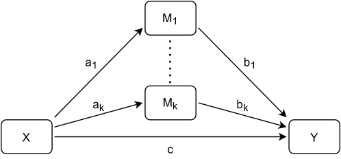
Figure 2: Diagram visualizing a parallel multiple mediator model.

2.1.2 Serial multiple mediator model

A distinctive feature of the serial multiple mediator model is that the hypothesized mediators $M_{1},\dots,M_{k}$ may influence each other in a sequential manner, unlike the parallel multiple mediator model in which the mediators do not affect one another. Figure 3 contains a diagram of the model with two serial mediators, while the model in its general form is given by

$$\begin{split}M_{1}&=i_{1}+a_{1}X+e_{1},\\ M_{2}&=i_{2}+d_{21}M_{1}+a_{2}X+e_{2},\\ &\hskip 5.0pt\vdots\\ M_{k}&=i_{k}+d_{k1}M_{1}+\dots+d_{k,k-1}M_{k-1}+a_{k}X+e_{k},\end{split}$$ (7)

$$Y =i_{k+1}+b_{1}M_{1}+\dots+b_{k}M_{k}+cX+e_{k+1},$$ (8)

$$Y =i_{k+2}+c^{\prime}X+e_{k+2},$$ (9)

where $i_{1},\dots,i_{k+2}$, $a_{1},\dots,a_{k}$, $d_{j1},\dots,d_{j,j-1}$, $j=2,\dots,k$, $b_{1},\dots,b_{k}$, $c$, and $c^{\prime}$ are regression coefficients to be estimated, and $e_{1},\dots,e_{k+2}$ are random error terms. It is easy to see that the serial multiple mediator model quickly grows in complexity with increasing number of mediators due to the combinatorial increase in indirect paths through the mediators (the number of indirect paths is given by $\sum_{j=1}^{k}{k\choose j}$ for $k$ serial mediators). In package robmed, it is therefore only implemented for two and three mediators to maintain a focus on easily interpretable models. Here, we only discuss the model for two serial mediators, and we refer to hayes18 for a diagram and a description of the various indirect effects in the case of three serial mediators.

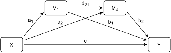
Figure 3: Diagram visualizing a serial multiple mediator model with two mediators.

For two serial mediators, the three indirect effects $a_{1}b_{1}$ ($X\rightarrow M_{1}\rightarrow Y$), $a_{2}b_{2}$ ($X\rightarrow M_{2}\rightarrow Y$), and $a_{1}d_{21}b_{2}$ ($X\rightarrow M_{1}\rightarrow M_{2}\rightarrow Y$) are the main parameters of interest. However, not all pairwise comparisons of the indirect effects may be meaningful (even if the mediators are scaled similarly), as $a_{1}d_{21}b_{2}$ can be expected to be different in magnitude from $a_{1}b_{1}$ and $a_{2}b_{2}$. Finally, we have that $c^{\prime}=a_{1}b_{1}+a_{2}b_{2}+a_{1}d_{21}b_{2}+c$ under the usual assumptions of independent and normally distributed error terms.

2.1.3 Multiple independent variables to be mediated

Instead of having multiple mediators, one can also allow for multiple independent variables $X_{1},\dots,X_{l}$ to influence the dependent variable $Y$ through a hypothesized mediator $M$. The resulting model is visualized in Figure 4 and defined by the equations

$$M =i_{1}+a_{1}X_{1}+\dots+a_{l}X_{l}+e_{1},$$ (10)

$$Y =i_{2}+bM+c_{1}X_{1}+\dots+c_{l}X_{l}+e_{2},$$ (11)

$$Y =i_{3}+c_{1}^{\prime}X_{1}+\dots+c_{l}^{\prime}X_{l}+e_{3},$$ (12)

where $i_{1},i_{2},i_{3}$, $a_{1},\dots,a_{l}$, $b$, $c_{1},\dots,c_{l}$, and $c_{1}^{\prime},\dots,c_{l}^{\prime}$ are regression coefficients to be estimated, and $e_{1}$, $e_{2}$, and $e_{3}$ are random error terms. The indirect effects $a_{1}b,\dots,a_{l}b$ are the main parameters of interest, and with the direct effects $c_{1},\dots,c_{l}$ and total effects $c_{1}^{\prime},\dots,c_{l}^{\prime}$, it holds that $c_{j}^{\prime}=a_{j}b+c_{j}$, $j=1,\dots,l$, under the usual independence and normality assumptions on the error terms. If the independent variables are on a comparable scale, it can also be of interest to make pairwise comparisons between the indirect effects or their absolute values.

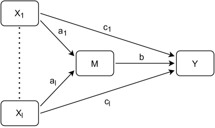
Figure 4: Diagram visualizing a mediation model with multiple independent variables.

This model is commonly used when the hypothesized mediator is the main (explanatory) variable of interest and its antecedents are being studied. Furthermore, an important special case of this model occurs when a categorical independent variable is represented by a group of dummy variables.

2.1.4 Control variables

In many study designs, it may be necessary to isolate the effects of the independent variables of interest from other factors. For instance, consider a study on whether exercise-induced feelings such as physical exhaustion mediate the relationship between physical activity and depression (cf. pickett12). If the participants vary in demographics such as age and gender, the researcher may need to control for the effects of those variables (e.g., older people may be less capable of engaging in strenuous activities; cerin09). Such control variables should be added to all regression equations of a mediation model. This means that there is no intrinsic difference between independent variables of interest and control variables in terms of the model or its estimation. The difference is purely conceptual in nature: for the control variables, the estimates of the direct and indirect paths are not of particular interest to the researcher. Package robmed therefore allows to specify control variables separately from the independent variables of interest. Only for the latter, results for the indirect effects are included in the output.

While we omitted control variables from the above equations and diagrams for notational simplicity, package robmed supports additional control variables in all implemented models.

2.1.5 More complex models

The models described above do not exist in isolation and some of them can be combined. For instance, robmed supports parallel and serial multiple mediator models with multiple independent variables of interest. Other variations of the mediation model, such as the moderated mediation and mediated moderation models (e.g., muller05) are out of scope for this paper. They are not yet implemented in package robmed but we aim to add support in future versions.

2.2 Overview of implemented methods

test	method	robust	family	Description	Simple mediation	Parallel mediators	Serial mediators	Multiple independent variables of interest	Control variables
"boot"	"regression"	"MM" or    TRUE		MM-regression (yohai87) and the fast-and-robust bootstrap (salibian02) are used to construct a confidence interval (alfons22a).	✓	✓	✓	✓	✓
"boot"	"regression"	"median"		A bootstrap confidence interval is computed based on median regressions (yuan14).	✓	✓	✓	✓	✓
"boot"	"regression"	FALSE	"gaussian"	A bootstrap confidence interval is computed based on OLS regressions (bollen90; shrout02; mackinnon04; preacher04; preacher08).	✓	✓	✓	✓	✓
"boot"	"regression"	FALSE	"select"	Regression models with normal, skew-normal, $t$, or skew-$t$ error distributions are estimated (azzalini13), and a bootstrap confidence interval is computed. The best fitting error distribution is selected via BIC.	✓	✓	✓	✓	✓
"boot"	"covariance"	TRUE		Following multivariate winsorization, a bootstrap confidence interval is computed for coefficient estimation via the maximum likelihood estimator of the covariance matrix (zu10).	✓
"boot"	"covariance"	FALSE		A bootstrap confidence interval is computed for coefficient estimation via the maximum likelihood estimator of the covariance matrix.	✓

Table 1: Overview of bootstrap procedures for mediation analysis implemented in the R package robmed, and corresponding argument values to use in function test_mediation().

test	method	robust	family	Description	Simple mediation	Parallel mediators	Serial mediators	Multiple independent variables of interest	Control variables
"sobel"	"regression"	"MM" or    TRUE		A variation of the Sobel test based on coefficient estimation via MM-regressions.	✓				✓
"sobel"	"regression"	"median"		A variation of the Sobel test based on coefficient estimation via median regressions.	✓				✓
"sobel"	"regression"	FALSE	"gaussian"	A variation of the Sobel test based on coefficient estimation via OLS regressions.	✓				✓
"sobel"	"regression"	FALSE	"select"	A variation of the Sobel test in which regression models with normal, skew-normal, $t$, or skew-$t$ error distributions are estimated, with the best fitting distribution being selected via BIC.	✓				✓
"sobel"	"covariance"	TRUE		Following multivariate winsorization, a variation of the Sobel test is applied based on coefficient estimation via the maximum likelihood estimator of the covariance matrix.	✓
"sobel"	"covariance"	FALSE		A variation of the Sobel test based on coefficient estimation via the maximum likelihood estimator of the covariance matrix.	✓

Table 2: Overview of variations of the Sobel test (sobel82) for mediation analysis implemented in the R package robmed, and corresponding argument values to use in function test_mediation(). Those tests are included for benchmarking purposes and are not recommended for empirical analyses.

While package robmed is focused on the fast-and-robust bootstrap procedure for mediation analysis introduced by alfons22a, various other methods are available as well. Tables 1 and 2 provide an overview of the available methods together with the corresponding argument values to use in function test_mediation(), which implements mediation analysis in robmed.

A bootstrap test is considered state-of-the art for mediation analysis, with many authors advocating to use the bootstrap with ordinary least-squares (OLS) estimation of the coefficients in the mediation model (bollen90; shrout02; mackinnon04; preacher04; preacher08). However, a bootstrap test can easily be applied to other methods of estimation. For instance, the mediation model can also be estimated via regressions with more flexible error distributions such as the skew-normal, $t$, or skew-$t$ distributions (see azzalini13, for maximum likelihood estimation of such regression models). Note that a similar procedure for mediation analysis, but using structural equation modeling, has been suggested in asparouhov16. Package robmed goes a step further in that it allows to select the best fitting error distribution via the Bayesian information criterion (BIC) (schwarz78). In addition, other robust methods for mediation analysis are implemented in robmed. yuan14 proposed a bootstrap test that replaces OLS estimation with median regression. zu10 proposed to first winsorize the data via a Huber M-estimator of the covariance matrix, and then to perform a bootstrap test on the cleaned data with coefficient estimation based on the maximum likelihood covariance matrix. A discussion of advantages and disadvantages of those approaches, as well as a comparison in extensive simulation studies, can be found in alfons22a.

Besides bootstrap tests, variations of the Sobel test (sobel82) are implemented in robmed. The Sobel test was originally proposed for maximum likelihood estimation of structural equation models, of which mediation models are a special case. It assumes a normal distribution of the indirect effect estimator and simplifies the calculation of the standard error by taking a first- or second-order approximation. This test has been criticized in the literature for its incorrect assumptions (e.g., mackinnon02), and a bootstrap test is generally preferred. Nevertheless, the Sobel test can easily be generalized to other estimation methods, and it is implemented in robmed for all estimation procedures of the (simple) mediation model. We emphasize that the Sobel tests are implemented for comparisons in benchmarking experiments and that they are not recommended for empirical analyses.

2.3 Fast-and-robust bootstrap test for mediation analysis

The robust procedure of alfons22a follows the state-of-the-art bootstrap approach for testing mediation (bollen90; shrout02; mackinnon04; preacher04; preacher08), but it replaces OLS regressions with the robust MM-estimator of regression (yohai87) and the standard bootstrap with the fast-and-robust bootstrap (salibian02; salibian08).

2.3.1 Robust regression

For a response variable $Y$, a $(p+1)$-dimensional random vector $\boldsymbol{X}$ in which the first component is fixed at 1, and a random error term $\varepsilon\sim N(0,\sigma^{2})$, the linear regression model is given by

$$Y=\boldsymbol{X}^{\top}\boldsymbol{\beta}+\varepsilon.$$

Denoting the corresponding observations by $(y_{i},\mathbf{x}_{i}^{\top})^{\top}$, $i=1,\dots,n$, the MM-estimate of regression with loss function $\rho$ (yohai87) is defined as

$$\boldsymbol{\hat{\beta}}_{n}=\mathop{\text{argmin}}_{\beta}\sum_{i=1}^{n}\rho\left(\frac{r_{i}(\boldsymbol{\beta})}{\hat{\sigma}_{n}}\right),$$ (13)

where $r_{i}(\boldsymbol{\beta})=y_{i}-\mathbf{x}_{i}^{\top}\boldsymbol{\beta}$, $i=1,\dots,n$, are the residuals, and $\hat{\sigma}_{n}$ is an initial estimate of the residual scale. We take $\hat{\sigma}_{n}$ from a highly robust but inefficient S-estimator of regression (rousseeuw84; salibian06), i.e.,

$$\hat{\sigma}_{n}=\min_{\boldsymbol{\beta}}\hat{\sigma}_{n}(\boldsymbol{\beta}),$$

where $\hat{\sigma}_{n}(\boldsymbol{\beta})$ is defined implicitly as the solution of

$$\frac{1}{n}\sum_{i=1}^{n}\rho_{S}\left(\frac{r_{i}(\boldsymbol{\beta})}{\hat{\sigma}_{n}(\boldsymbol{\beta})}\right)=\delta$$

with loss function $\rho_{S}$ and $\delta=E\left[\rho_{S}\left(\frac{X}{\sigma}\right)\right]$ for a random variable $X\sim N(0,\sigma^{2})$. For both $\rho$ and $\rho_{S}$, we use Tukey’s bisquare loss function defined as

$$\rho(x)=\left\{\begin{array}[]{ll}\displaystyle\frac{x^{6}}{6c^{4}}-\frac{x^{4}}{2c^{2}}+\frac{x^{2}}{2},&\text{if }|x|\leq c\\ \vskip 3.0pt plus 1.0pt minus 1.0pt\cr\displaystyle\frac{c^{2}}{6},&\text{if }|x|>c.\end{array}\right.$$ (14)

The value of the tuning constant $c$ in $\rho_{S}$ determines the robustness of the MM-estimator, and the value of $c$ in $\rho$ determines the efficiency (cf. yohai87). By default, we set $c=1.54764$ in $\rho_{S}$ for maximal robustness and $c=3.443689$ in $\rho$ for 85% efficiency at the model with normally distributed errors.

Taking the derivative of the objective function in (13) and equating the derivative to $\boldsymbol{0}$ yields the system of equations

$$\sum_{i=1}^{n}\rho^{\prime}\left(\frac{r_{i}(\boldsymbol{\beta})}{\hat{\sigma}_{n}}\right)\mathbf{x}_{i}=\boldsymbol{0}.$$ (15)

With weights

$$w_{i}=\frac{\rho^{\prime}(r_{i}(\boldsymbol{\beta})/\hat{\sigma}_{n})}{r_{i}(\boldsymbol{\beta})/\hat{\sigma}_{n}},\qquad i=1,\dots,n,$$

the system of equations in (15) can be rewritten as a weighted version of the normal equations:

$$\sum_{i=1}^{n}w_{i}r_{i}(\boldsymbol{\beta})\mathbf{x}_{i}=\boldsymbol{0}.$$ (16)

Therefore, the MM-estimator can be seen as a weighted least-squares estimator with data-dependent weights. Those weights indicate how much each observation deviates, as an observation with a large residual (large deviation) receives a weight of 0 or close to 0, while an observation with a small residual (small deviation) receives a weight close to 1. The loss function from (14) and the resulting weight function are displayed in Figure 5, which also includes the loss function and weight function from OLS regression for comparison.

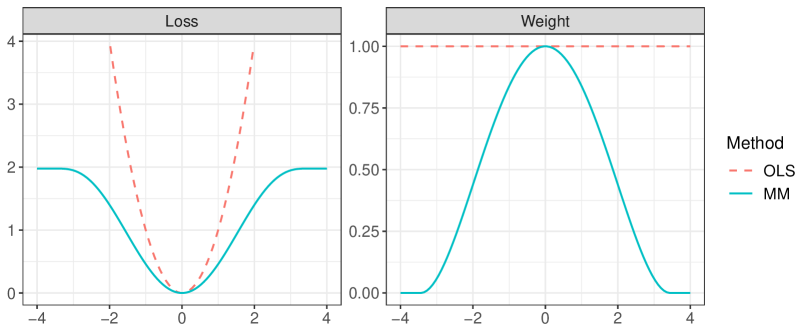
Figure 5: Loss function (left) and corresponding weight function (right) for OLS regression and the robust MM-estimator of regression.

2.3.2 Fast-and-robust bootstrap

Here we briefly present the main idea of the fast-and-robust bootstrap. For a detailed discussion and complete derivations, the reader is referred to salibian02 and salibian08. There are two concerns with bootstrapping robust estimators:

1. Outliers may be oversampled in some bootstrap samples to the extent that those samples contain more outliers than the robust estimator can handle, in which case bootstrap confidence intervals become unreliable.

2. Robust estimators typically have higher computational complexity than their nonrobust counterparts, which is amplified when computing many bootstrap replicates.

In many empirical applications of mediation analysis, the first concern is unlikely to be an issue when using the MM-estimator of regression due to its high robustness. We therefore use the fast-and-robust bootstrap mainly for its computational efficiency, although the extra robustness does provide additional peace of mind.

To derive the fast-and-robust bootstrap for the MM-estimator, note that the solution of (16) can be written as

$$\boldsymbol{\hat{\beta}}_{n}=\left(\sum_{i=1}^{n}w_{i}\mathbf{x}_{i}\mathbf{x}_{i}^{\top}\right)^{-1}\sum_{i=1}^{n}w_{i}\mathbf{x}_{i}y_{i}.$$

For a bootstrap sample $(y_{i}^{*},{\mathbf{x}_{i}^{*}}^{\top})^{\top}$, $i=1,\dots,n$, one can compute $r_{i}^{*}=y_{i}^{*}-{\mathbf{x}_{i}^{*}}^{\top}\boldsymbol{\hat{\beta}}_{n}$ and $w_{i}^{*}=\rho^{\prime}(r_{i}^{*}/\hat{\sigma}_{n})/(r_{i}^{*}/\hat{\sigma}_{n})$ for $i=1,\dots,n$. It is important to note that $\boldsymbol{\hat{\beta}}_{n}$ and $\hat{\sigma}_{n}$ are computed in advance on the original sample such that the robustness weights $w_{i}^{*}$ are inherited from the respective observations in the original sample. Then only a weighted least-squares fit is computed on the bootstrap sample to obtain

$$\boldsymbol{\hat{\beta}}_{n}^{\text{WLS}}=\left(\sum_{i=1}^{n}w_{i}^{*}\mathbf{x}_{i}^{*}{\mathbf{x}_{i}^{*}}^{\top}\right)^{-1}\sum_{i=1}^{n}w_{i}^{*}\mathbf{x}_{i}^{*}y_{i}^{*}.$$ (17)

However, using (17) for the bootstrap distribution would not capture all the variability in the MM-estimator, as the robustness weights are not recomputed on the bootstrap samples. Nevertheless, a linear correction of the coefficients can be applied to overcome this loss of variability. The correction matrix only needs to be computed once based on the original sample and is given by

$$\boldsymbol{K}_{n}=\left(\sum_{i=1}^{n}\rho^{\prime\prime}(r_{i}/\hat{\sigma}_{n})\mathbf{x}_{i}\mathbf{x}_{i}^{\top}\right)^{-1}\sum_{i=1}^{n}w_{i}\mathbf{x}_{i}\mathbf{x}_{i}^{\top}.$$

Then the fast-and-robust bootstrap replicate on the given bootstrap sample is computed as

$$\boldsymbol{\hat{\beta}}_{n}^{*}=\boldsymbol{\hat{\beta}}_{n}+\boldsymbol{K}_{n}\left(\boldsymbol{\hat{\beta}}_{n}^{\text{WLS}}-\boldsymbol{\hat{\beta}}_{n}\right).$$ (18)

Since the MM-estimator $\boldsymbol{\hat{\beta}}_{n}$ is consistent for $\boldsymbol{\beta}$ (yohai87), $\sqrt{n}(\boldsymbol{\hat{\beta}}_{n}^{*}-\boldsymbol{\hat{\beta}}_{n})$ has the same asymptotic distribution as $\sqrt{n}(\boldsymbol{\hat{\beta}}_{n}-\boldsymbol{\beta})$ (salibian08; salibian02).

2.3.3 Bootstrapping the indirect effects in mediation analysis

For simplicity, we focus on the indirect effect in the simple mediation model from (1)–(3). Similar calculations apply to the indirect effects in the mediation models described in Section 2.1. On each bootstrap sample, (18) is used to obtain estimates $\hat{a}$, $\hat{b}$, and $\hat{c}$ of the coefficients in (1) and (2), and therefore estimates $\hat{a}\hat{b}$ of the indirect effect. Note that we do not perform the regression corresponding to (3) and instead estimate the total effect by $\hat{c}^{\prime}=\hat{a}\hat{b}+\hat{c}$. With the empirical distribution of the indirect effect over the bootstrap samples, we construct a percentile-based confidence interval. By default, we report a bias-corrected and accelerated confidence interval (davison97). Furthermore, we advocate to report the mean over the bootstrap distribution as the final point estimates of the indirect effect.

3 Package contents and implementation

We describe the included data set in Section 3.1, introduce the formula interface for specifying mediation models in Section 3.2, and briefly discuss the main functions as well as the class structure of package robmed in Section 3.3. Moreover, we load the package and the data in order to use them in code examples. R> library("robmed") R> data("BSG2014")

3.1 Example data

The BSG2014 data included in package robmed come from a business simulation game that was played by senior business administration students as part of a course at a Western European university. The simulation game was played twice, and a survey was conducted in three waves (before the first game, in between the two games, and after the second game). A total of 354 students formed 92 randomly assigned teams, and the responses of the individual students were aggregated to the team level. Leaving out teams with less than 50 percent response rate yields a sample size of $n=89$ teams.

Below, we provide an overview of the variables that are used later on in the case studies in Section 4. For a complete description of the data, we refer to its R help file, which can be accessed from the console with ?BSG2014.

ValueDiversity: Using the short Schwartz’s value survey (lindeman05), the team members rated ten items on the importance of certain values (1 = not important, 10 = highly important). For each value item, the coefficient of variation of the individual responses across team members was computed, and the resulting coefficients of variation were averaged across the value items.

TaskConflict: Using the intra-group conflict scale of jehn95, the team members rated four items on the presence of conflict regarding the work on a 5-point scale (1 = none, 5 = a lot). The individual responses were aggregated by taking the average across items and team members.

TeamCommitment: The team members indicated the extent to which they agree or disagree with four items on commitment to the team, which are based on mowday79, using a 5-point scale (1 = strongly disagree, 5 = strongly agree). The individual responses were aggregated by taking the average across items and team members.

TeamScore: The team performance scores on the second game were computed at the end of the simulation through a mix of five objective performance measures: return on equity, earnings-per-share, stock price, credit rating, and image rating. The computation of the scores is handled by the simulation game software, and details can be found in mathieu09.

SharedLeadership: Following carson07, every team member assessed each of their peers on the question of “To what degree does your team rely on this individual for leadership?” using a 5-point scale (1 = not at all, 5 = to a very large extent). The leadership ratings were aggregated by taking the sum and dividing it by the number of pairwise relationships among team members.

AgeDiversity: Following harrison07, age diversity was operationalized by the coefficient of variation of the team members’ ages.

GenderDiversity: Gender diversity was measured with Blau’s index, $1-\sum_{j}p_{j}^{2}$, where $p_{j}$ is the proportion of team members in the $j$-th category (blau77).

ProceduralJustice: Based on the intra-unit procedural justice climate scale of li09, the team members indicated the extent to which they agree or disagree with four items on a 5-point scale (1 = strongly disagree, 5 = strongly agree). The individual responses were aggregated by taking the average across items and team members.

InteractionalJustice: Using the intra-unit interactional justice climate scale of li09, the team members indicated the extent to which they agree or disagree with four items on a 5-point scale (1 = strongly disagree, 5 = strongly agree). The individual responses were aggregated by taking the average across items and team members.

TeamPerformance: Following hackman86, the team members indicated the extent to which they agree or disagree with four items on the team’s functioning, using a 5-point scale (1 = strongly disagree, 5 = strongly agree). The individual responses were aggregated by taking the average across items and team members.

To gain some insight into the distribution of those variables (including their ranges), we extract them from the data set and produce a summary: R> keep <- c("ValueDiversity", "TaskConflict", "TeamCommitment", "TeamScore", + "SharedLeadership", "AgeDiversity", "GenderDiversity", + "ProceduralJustice", "InteractionalJustice", "TeamPerformance") R> summary(BSG2014[, keep]) ValueDiversity TaskConflict TeamCommitment TeamScore Min. :1.105 Min. :1.125 Min. :2.125 Min. : 49.00 1st Qu.:1.443 1st Qu.:1.500 1st Qu.:3.625 1st Qu.: 90.00 Median :1.587 Median :1.688 Median :3.875 Median : 98.00 Mean :1.676 Mean :1.761 Mean :3.822 Mean : 95.72 3rd Qu.:1.916 3rd Qu.:2.000 3rd Qu.:4.125 3rd Qu.:104.00 Max. :2.548 Max. :2.938 Max. :4.688 Max. :110.00 SharedLeadership AgeDiversity GenderDiversity ProceduralJustice Min. :3.500 Min. :0.0000 Min. :0.0000 Min. :3.375 1st Qu.:6.333 1st Qu.:0.5000 1st Qu.:0.0000 1st Qu.:3.750 Median :6.667 Median :0.8165 Median :0.3750 Median :3.875 Mean :6.629 Mean :0.9723 Mean :0.3031 Mean :3.908 3rd Qu.:7.167 3rd Qu.:1.2583 3rd Qu.:0.3750 3rd Qu.:4.062 Max. :9.333 Max. :4.2720 Max. :0.5000 Max. :4.500 InteractionalJustice TeamPerformance Min. :3.312 Min. :3.000 1st Qu.:4.167 1st Qu.:3.667 Median :4.375 Median :4.000 Mean :4.379 Mean :3.968 3rd Qu.:4.625 3rd Qu.:4.250 Max. :5.000 Max. :4.750 For instance, the objective team performance scores in variable TeamScore range from $49$ to $110$.

3.2 Formula interface

The equations in the mediation model follow a specific structure regarding which variable is used as the response variable and which variables are the explanatory variables. Some R packages for mediation analysis, e.g., mediation (tingley14), require the user to specify one formula for each equation, which can be tedious and prone to mistakes, in particular for models with multiple mediators and multiple independent variables or control variables. Other packages, e.g., psych (psych) or MBESS (MBESS), do not provide a formula interface at all, despite formulas being the standard way of describing models in R.

For package robmed, we designed a formula interface that builds upon the standard formula interface in R, but allows to specify the mediation model with a single formula. As usual, the dependent variable is defined on the left hand side of the formula, and the independent variable is given on the right hand side. In addition, the functions m() and covariates() can be used on the right hand side to define the hypothesized mediators and any control variables, respectively. If multiple mediators are supplied, function m() provides the argument .model, which accepts the values "parallel" for parallel mediators (the default) and "serial" for serial mediators. The corresponding wrapper functions parallel_m() and serial_m() are available for convenience.

For example, a simple mediation model can be defined as follows (see also the case study in Section 4.1): R> TeamCommitment   m(TaskConflict) + ValueDiversity An example for a serial multiple mediator model is specified with the following formula (see also the case study in Section LABEL:sec:serial), where the serial mediators are listed in consecutive order from left to right: R> TeamScore   serial_m(TaskConflict, TeamCommitment) + ValueDiversity The formula specification for an example of a parallel multiple mediator model with control variables is given by (see also the case study in Section LABEL:sec:parallel): R> TeamPerformance   parallel_m(ProceduralJustice, InteractionalJustice) + + SharedLeadership + covariates(AgeDiversity, GenderDiversity) Note that different variables within m(), parallel_m(), serial_m(), and covariates() are separated by commas.

3.3 Main functions and class structure

The two main functions of package robmed are fit_mediation(), which implements various methods for the estimation of a mediation model, and test_mediation(), which performs statistical tests on the indirect effects in the mediation model. Furthermore, robmed follows a clear object-oriented design using S3 classes (chambers92).

Function fit_mediation() is mainly intended to be used internally by test_mediation(), but it is also useful for a user who wants to compare different tests on the indirect effects for the same method of estimation, such that the estimation on the given sample only has to be performed once. It returns an object inheriting from class "fit_mediation". The currently available subclasses are "reg_fit_mediation" if the mediation model was estimated via a series of regressions, and "cov_fit_mediation" if the model was estimated based on the covariance matrix of the involved variables.

We expect most users to find it more convenient to use test_mediation() directly in order to perform model estimation and testing the indirect effects with one function call. See Tables 1 and 2 for an overview of which argument values to use in test_mediation() for the various available methods. Furthermore, function robmed() is a wrapper function for the fast-and-robust bootstrap test of alfons22a. The results are returned as an object inheriting from class "test_mediation". The currently available subclasses are "boot_test_mediation" for bootstrap tests, and "sobel_test_mediation" for tests based on the normal approximation of sobel82. Among other information, the component fit stores the estimation results as an object inheriting from class "fit_mediation". Objects of class "boot_test_mediation" also contain a component reps, which stores the bootstrap replicates as an object of class "boot", as returned by function boot() from package boot (boot). It should be noted that the internal use of function boot() implies that the user can easily take advantage of parallel computing to reduce computation time.

Functions fit_mediation() and test_mediation() are implemented as generic functions. Two methods are available for both functions: one method uses the formula interface described in Section 3.2, while the default method provides an alternative way of specifying mediation models. Additionally, test_mediation() has a method for objects inheriting from class "fit_mediation", as returned by fit_mediation(). The default methods take the data set as their first argument in order to work nicely with the pipe operator, i.e., |> introduced in R version 4.1.0 or %>% from package magrittr (magrittr). Arguments x, y, m, and covariates take character, integer, or logical vectors to select the independent variables, the dependent variable, the hypothesized mediators, and any additional control variables, respectively, from the data set. Note that this interface offers various ways to select the variables in a programmable manner. In case of multiple mediators, argument model allows to specify whether multiple mediators are treated as parallel or serial mediators.

Package robmed provides various accessor functions to extract relevant information from the returned objects, such as coef() and confint() methods. In addition, it contains the plot functions weight_plot() and ellipse_plot() for diagnostics, as well as ci_plot() to visualize confidence intervals and density_plot() to plot density estimates of the indirect effect estimators.

4 Illustrations: Using package robmed

We demonstrate the use of package robmed in three illustrative mediation analyses using the included data set BSG2014 (see Section 3.1). While the package and the data have already been loaded in Section 3, we store the seed to be used for the random number generator in an object, as it will be needed in all examples for the purpose of replicating the results. R> seed <- 20211117

The following subsections provide examples for a simple mediation model (Section 4.1), a serial multiple mediator model (Section LABEL:sec:serial), as well as a parallel multiple mediator model with additional control variables (Section LABEL:sec:parallel).

4.1 Simple mediation

In the first code example, we replicate parts of the empirical example of alfons22a. The illustrative hypothesis to be investigated is that task conflict mediates the relationship between team value diversity and team commitment. Using robmed’s formula interface (see Section 3.2), we specify a simple mediation model with the dependent variable TeamCommitment on the left hand side. On the right hand side, we have the hypothesized mediator TaskConflict, which is wrapped in a call to function m(), as well as the independent variable ValueDiversity. As we will compare the robust bootstrap test of alfons22a with the OLS bootstrap test (e.g., preacher04; preacher08; hayes18), we store the formula object for later use. R> f_simple <- TeamCommitment   m(TaskConflict) + ValueDiversity

Next, we perform the two bootstrap tests using function test_mediation(). As usual for functions that fit models, we supply the model specification and the data via the formula and data arguments. By default, test_mediation() fits the mediation model via regressions (argument method = "regression") and performs a bootstrap test for the indirect effect (argument test = "boot") with 5000 bootstrap replications (argument R = 5000). In that case, setting robust = TRUE (the default) or robust = "MM" specifies the robust bootstrap procedure of alfons22a, while robust = FALSE yields the nonrobust OLS bootstrap test. Before each call to test_mediation(), we set the seed of the random number generator. R> set.seed(seed) R> robust_boot_simple <- test_mediation(f_simple, data = BSG2014, + robust = TRUE) R> set.seed(seed) R> ols_boot_simple <- test_mediation(f_simple, data = BSG2014, + robust = FALSE) Other estimation methods for a bootstrap test can be specified via a combination of arguments, as outlined in Table 1.

Function test_mediation() returns an object inheriting from class "test_mediation". The corresponding summary() method shows the relevant information on the fitted models and emphasizes the significance tests of the total, direct, and indirect effects. For bootstrap tests, the information displayed by summary() by default stays within the bootstrap framework. For effects other than the indirect effect, asymptotic tests are performed using the normal approximation of the bootstrap distribution. That is, the sample mean and the sample standard deviation of the bootstrap replicates are used for asymptotic $z$ tests. Furthermore, bootstrap estimates of all effects are shown in addition to the estimates on the original data. At the bottom of the output, the indirect effect is summarized by the estimate on the original data (column Data), the bootstrap estimate (i.e., the sample mean of the bootstrap replicates; column Boot), and the lower and upper limits of the confidence interval (columns Lower and Upper, respectively). R> summary(robust_boot_simple) Robust bootstrap test for indirect effect via regression

x = ValueDiversity y = TeamCommitment m = TaskConflict

Sample size: 89 — Outcome variable: TaskConflict

Coefficients: Data Boot Std. Error z value Pr(>|z|) (Intercept) 1.1182 1.1174 0.1798 6.214 5.16e-10 *** ValueDiversity 0.3197 0.3208 0.1071 2.996 0.00274 **

Robust residual standard error: 0.3033 on 87 degrees of freedom Robust R-squared: 0.1181, Adjusted robust R-squared: 0.108 Robust F-statistic: 9.113 on 1 and Inf DF, p-value: 0.002539

Robustness weights: 4 observations are potential outliers with weight <= 1.3e-05: [1] 48 58 76 79 — Outcome variable: TeamCommitment

Coefficients: Data Boot Std. Error z value Pr(>|z|) (Intercept) 4.33385 4.33515 0.34415 12.597 <2e-16 *** TaskConflict -0.33659 -0.33672 0.17759 -1.896 0.058 . ValueDiversity 0.06523 0.06388 0.18593 0.344 0.731

Robust residual standard error: 0.3899 on 86 degrees of freedom Robust R-squared: 0.08994, Adjusted robust R-squared: 0.06878 Robust F-statistic: 1.497 on 2 and Inf DF, p-value: 0.2239

Robustness weights: Observation 6 is a potential outlier with weight 0 — Total effect of x on y: Data Boot Std. Error z value Pr(>|z|) ValueDiversity -0.04239 -0.04293 0.18704 -0.23 0.818

Direct effect of x on y: Data Boot Std. Error z value Pr(>|z|) ValueDiversity 0.06523 0.06388 0.18593 0.344 0.731

Indirect effect of x on y: Data Boot Lower Upper TaskConflict -0.1076 -0.1068 -0.2936 -0.009158 — Level of confidence: 95

Number of bootstrap replicates: 5000 — Signif. codes: 0 ’***’ 0.001 ’**’ 0.01 ’*’ 0.05 ’.’ 0.1 ’ ’ 1

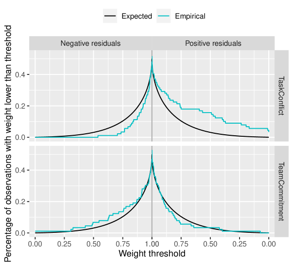
Figure 6: Diagnostic plot of the regression weights from the robust bootstrap procedure of alfons22a.

The above results are very similar to those reported in alfons22a, but they are not identical due to a change in the random number generator in R and the use of a different seed. Specifically, the robust bootstrap test detects a significant indirect effect, as the confidence interval is strictly negative. This negative indirect effect is composed of a positive effect of value diversity on task conflict (see the output of the first regression model), and a negative effect of task conflict on team commitment (see the output of the second regression model). For further interpretation, recall that value diversity is measured as a coefficient of variation averaged over various value dimensions, and that task conflict and team commitment are measured as averages of items on a 5-point rating scale. On average, an increase in value diversity by one relative standard deviation explains an increase in task conflict by about 0.32 points, which in turn explains a decrease in team commitment by about 0.11 points. Furthermore, we observe that the direct effect of value diversity on team commitment is not significantly different from 0, meaning that value diversity affects team commitment only via the indirect path through task conflict. In the typology of mediations of zhao10, we find indirect-only mediation.

Note that the output corresponding to the regression models is similar to that of the summary() method for "lmrob" objects from package robustbase (robustbase), but it is shortened as the output is already rather long. In particular, we emphasize that the indices of potential outliers are displayed for each regression model. Those potential outliers should always be investigated further, as they may be interesting observations that could lead to new insights when studied separately (see alfons22a, for a detailed discussion on outliers in the mediation model).

Moreover, when the summary output for the robust bootstrap procedure of alfons22a is printed, by default also a diagnostic plot is shown that allows to detect deviations from normality assumptions. Keep in mind that this procedure uses the robust MM-estimator of regression (yohai87; salibian02), which assigns robustness weights to all observations. Those weights can take any value in the interval $[0,1]$, with lower values indicating a higher degree of deviation. For a varying threshold on the horizontal axis, the diagnostic plot displays how many observations have a weight below this threshold. The plot is thereby split into separate panels for negative and positive residuals. For comparison, a reference line is drawn for the expected percentages under normally distributed errors.

Figure 6 shows the plot for this example. For the regression of the hypothesized mediator (TaskConflict) on the independent variable in the top row of the plot, it reveals much more downweighted observations with positive residuals than expected and fewer with negative residuals. This indicates right skewness with a heavy upper tail.

It is possible to suppress the plot by setting plot = FALSE in summary(). Then function weight_plot() can be used to create the diagnostic plot. In this example, Figure 6 can also be produced with the commands below. R> weight_plot(robust_boot_simple) + + scale_color_manual("", values = c("black", "#00BFC4")) + + theme(legend.position = "top")

It should also be noted that the output from summary() is structured in a similar way as the output of the widely-used macro PROCESS (hayes18), which implements the OLS bootstrap test for conditional process models such as the mediation model. The intention is to facilitate the use of package robmed for users of the PROCESS macro. While PROCESS constructs a bootstrap confidence interval for the indirect effect, it reports estimates on the original data and the usual normal-theory $t$ tests for all other effects. In robmed, the same can be achieved by setting the argument type = "data" in the summary() method. The results from the regressions are then summarized in the usual way, as shown below for the OLS bootstrap. R> summary(ols_boot_simple, type = "data") Bootstrap test for indirect effect via regression

x = ValueDiversity y = TeamCommitment m = TaskConflict

Sample size: 89 — Outcome variable: TaskConflict

Coefficients: Estimate Std. Error t value Pr(>|t|) (Intercept) 1.5007 0.2069 7.253 1.59e-10 *** ValueDiversity 0.1552 0.1209 1.283 0.203

Residual standard error: 0.3908 on 87 degrees of freedom Multiple R-squared: 0.01857, Adjusted R-squared: 0.007289 F-statistic: 1.646 on 1 and 87 DF, p-value: 0.2029 — Outcome variable: TeamCommitment

Coefficients: Estimate Std. Error t value Pr(>|t|) (Intercept) 4.49846 0.28806 15.616 < 2e-16 *** TaskConflict -0.36412 0.11783 -3.090 0.00269 ** ValueDiversity -0.02088 0.13418 -0.156 0.87671

Residual standard error: 0.4296 on 86 degrees of freedom Multiple R-squared: 0.1031, Adjusted R-squared: 0.08227 F-statistic: 4.944 on 2 and 86 DF, p-value: 0.009279 — Total effect of x on y: Estimate Std. Error t value Pr(>|t|) ValueDiversity -0.07738 0.13930 -0.555 0.58

Direct effect of x on y: Estimate Std. Error t value Pr(>|t|) ValueDiversity -0.02088 0.13418 -0.156 0.877

Indirect effect of x on y: Data Boot Lower Upper TaskConflict -0.0565 -0.05838 -0.2137 0.02458 — Level of confidence: 95

Number of bootstrap replicates: 5000 — Signif. codes: 0 ’***’ 0.001 ’**’ 0.01 ’*’ 0.05 ’.’ 0.1 ’ ’ 1 Unlike the robust bootstrap test above, the OLS bootstrap does not detect a significant indirect effect, since the confidence interval covers 0. Due to the influential heavy tail indicated by the diagnostic plot in Figure 6, the results of the robust bootstrap test can be considered more reliable.

Methods for common generic functions to extract information from objects are implemented in robmed, such as a coef() method to extract the relevant effects of the mediation model, and confint() to extract confidence intervals of those effects. R> coef(robust_boot_simple) a b Total Direct Indirect 0.32077184 -0.33672132 -0.04292728 0.06388476 -0.10681204 R> confint(robust_boot_simple) 2.5 a 0.1109227 0.530620997 b -0.6847919 0.011349287 Total -0.4095137 0.323659113 Direct -0.3005305 0.428300051 Indirect -0.2936367 -0.009158447 While the confidence intervals in this example do not add much in terms of interpretation over the output of summary(), the latter reports significance tests instead of confidence intervals for the effects other than the indirect effect. For researchers who prefer to report confidence intervals, the confint() method allows to easily extract this information.

For objects corresponding to bootstrap tests (class "boot_test_mediation"), argument type of the coef() method allows to specify whether to extract the bootstrap estimates ("boot", the default) or the estimates on the original data ("data"). Similarly, argument type of the confint() method allows to specify whether the confidence intervals for the effects other than the indirect effect should be bootstrap confidence intervals ("boot", the default) or normal theory intervals based on the original data ("data"). R> coef(ols_boot_simple, type = "data") a b Total Direct Indirect 0.15517748 -0.36412398 -0.07738318 -0.02087934 -0.05650384 R> confint(ols_boot_simple, type = "data") 2.5 a -0.08521602 0.3955710 b -0.59836363 -0.1298843 Total -0.35426561 0.1994992 Direct -0.28761575 0.2458571 Indirect -0.21371944 0.0245833 In addition, argument parm allows to specify which coefficients or confidence intervals to extract.