Self-Supervised Transformers for Unsupervised Object Discovery using Normalized Cut

Abstract

Transformers trained with self-supervision using self-distillation loss (DINO) have been shown to produce attention maps that highlight salient foreground objects. In this paper, we show a graph-based method that uses the self-supervised transformer features to discover an object from an image. Visual tokens are viewed as nodes in a weighted graph with edges representing a connectivity score based on the similarity of tokens. Foreground objects can then be segmented using a normalized graph-cut to group self-similar regions. We solve the graph-cut problem using spectral clustering with generalized eigen-decomposition and show that the second smallest eigenvector provides a cutting solution since its absolute value indicates the likelihood that a token belongs to a foreground object.

Despite its simplicity, this approach significantly boosts the performance of unsupervised object discovery: we improve over the recent state-of-the-art LOST by a margin of 6.9%, 8.1%, and 8.1% respectively on the VOC07, VOC12, and COCO20K. The performance can be further improved by adding a second stage class-agnostic detector (CAD). Our proposed method can be easily extended to unsupervised saliency detection and weakly supervised object detection. For unsupervised saliency detection, we improve IoU for 4.9%, 5.2%, 12.9% on ECSSD, DUTS, DUT-OMRON respectively compared to state-of-the-art. For weakly supervised object detection, we achieve competitive performance on CUB and ImageNet. Our code is available at: https://www.m-psi.fr/Papers/TokenCut2022/

1 Introduction

(a) DINO [6]

(b) LOST [45].

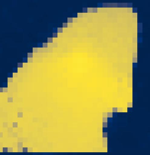
(c) TokenCut (ours)

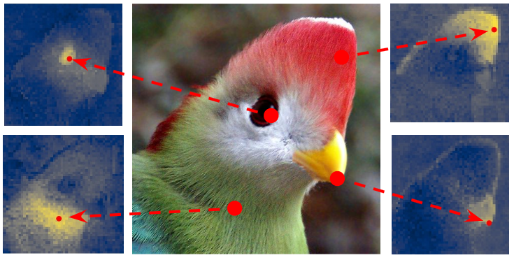
(d) Attention maps associated to different patches

Figure 1: The attention map of the class token used in DINO [6] (a) and the map of the inverse degrees used in LOST [45] (b) are noisy for foreground / background separation. Our proposed method provides a clean attention map that can be used to segment salient objects (c). Considering the attention map associated to different patches highlight different regions of the object (d), it is reasonable to build a graph computing attention maps from multiple patches.

Object detection is a key enabling technology for real-world vision systems for tasks such as robotics, autonomous driving, traffic monitoring, manufacturing, and embodied artificial intelligence  [63, 21, 64]. However, the performance of current state-of-the-art object detectors is limited by the high cost of annotating sufficient training data [33] for supervised learning. This limitation becomes even more apparent when using transfer learning to adapt a pre-trained object detector to a new application domain. Approaches such as active learning [1], semi-supervised learning [34], and weakly-supervised learning [39] have attempted to overcome this barrier by providing more efficient learning, but with only limited success.

In this work, we focus on object discovery in natural images with no human annotations. This is an important problem and a critical step for many downstream applications [56]. Poor object discovery can lead to poor overall system performance. Current approaches for this problem adopt some forms of bounding box proposal mechanism [11, 61, 56, 55] and formulate object discovery as an optimization problem. However, this approach can be computationally expensive [55] as each pair of bounding box proposals across different images needs to be compared, and the optimization may fail to scale to larger datasets due to the quadratic computation overhead [57].

Transformers have recently been shown to outperform convolutional neural networks for visual recognition. Vision Transformers, such as ViT [18] accept image patches as input tokens and use stacked layers of encoders with self-attention to map tokens to image-level class labels. Recent results with DINO [6] have shown that when trained with self-distillation loss [25], the attention maps associated to the class token from the last layer indicate salient foreground regions. However, as illustrated in Fig. 1a, such attention maps are noisy and it is not clear that they can be used for unsupervised object discovery.

With LOST [45], the authors propose construction of a graph and use the inverse degrees of nodes to segment objects. A heuristic seed expansion strategy is used to overcome noise (Fig. 1b) and detect a single bounding box for a foreground object. The attention maps associated with different nodes often contain meaningful information, as illustrated in Fig. 1d. We have investigated whether it is possible to use the information in the entire graph by projecting the graph into a low dimensional subspace using eigendecomposition. We have discovered that such a projection can be used with Normalized Cut [43] (Ncut) to significantly improve foreground / background segmentation (Fig. 1c).

In this paper, we propose TokenCut, a simple but effective graph-based approach for unsupervised object discovery. We build on the self-supervised vision transformer trained with DINO [6] as our backbone feature encoder and locate objects with the resulting features. Instead of using only the class token, we use all token features. We construct an undirected graph based on the token features in the last self-attention layer, where the visual tokens are viewed as graph nodes with edges representing a connectivity score based on similarity of the features. We then use a normalized graph-cut to group self-similar regions and delimit the foreground objects. We solve the graph-cut problem using spectral clustering with generalized eigen-decomposition and show that the second smallest eigenvector provides a cutting solution indicating the likelihood that a token belongs to a foreground object. Our approach can be considered as a run-time adaptation, which means that the model is able to adapt to each specific test image despite the shared training model.

Despite its simplicity, our approach significantly improves unsupervised object discovery. The method achieves 68.8%, 72.1% and 58.8% on VOC07 [19], VOC12 [20], COCO20K [33] respectively, thus outperforming LOST [45] by a margin of 6.9%, 8.1% and 8.1% respectively. TokenCut with second stage CAD further improves the performance to 71.4%, 75.3% and 62.6% on VOC07, VOC12, COCO20k respectively, which outperforms LOST + CAD by 5.7%, 4.9% and 5.1% respectively.

In addition, we show that TokenCut can be easily extended to weakly supervised object detection and unsupervised saliency detection. For weakly supervised object detection, the goal is to detect objects using only image-level annotations. We freeze the encoder and fine-tune a linear classifier with weakly-supervised image labels. We then apply TokenCut on the features extracted from the fine-tuned encoder. Our approach produces clearly improved results on the CUB dataset [59] and competitive performance on ImageNet-1K [14]. For unsupervised saliency detection, we use the foreground region discovered by the proposed approach and apply Bilateral Solver [5] as a post-processing step to refine edges of the foreground region. In terms of results, our approach significantly improves previous state-of-the-art methods on ECSSD [44], DUTS [60] and DUT-OMRON [67].

In summary, our main contributions are as follows:

• We propose a simple and effective method to discover objects in images without supervision based on the self-supervised vision transformers. This method significantly outperforms previous state-of-the-art methods for unsupervised object discovery when tested on multiple datasets;

• We extend the proposed method to weakly-supervised object detection and show that the simple approach can achieve competitive performance;

• We also show that this method can be used for unsupervised saliency detection. The results demonstrate that TokenCut significantly improves the previous state-of-the-art performance on multiple datasets.

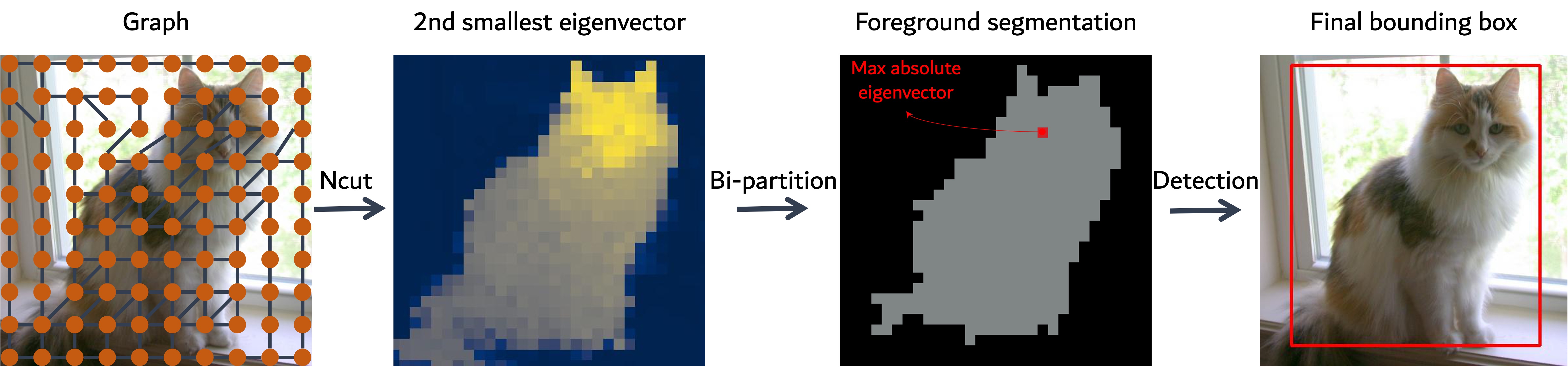
Figure 2: An overview of the TokenCut approach. We construct a graph where the nodes are tokens and the edges are similarities between the tokens using transformer features. The foreground and background segmentation can be solved by Ncut [43]. Performing bi-partition on the second smallest eigenvector allows to detect foreground object.

2 Related Work

Self-supervised vision transformers.

ViT [18] has shown that a transformer architecture [53] can be used as an effective encoder for images and provide useful features for supervised vision tasks. MoCo-v3 [8] demonstrated that ViT can provide self-supervised representation learning and achieve strong results using contrastive learning. Recently, DINO [6] proposed to train transformers with self-distillation loss [25], showing that ViT contains explicit information that can be used for semantic segmentation of an image. Inspired by BERT [16], [32] proposed MST, which dynamically masks some tokens and learns to recover missing tokens using a global image decoder. Also motivated by BERT [16], BEIT [4] first tokenizes the original image into visual tokens then randomly mask some tokens and learn to recover them using a transformer. Recently, MAE [23] masks a high proportion of images and reconstructs the missing pixels with an asymmetric encoder-decoder.

Unsupervised object discovery.

Given a group of images, unsupervised object discovery seeks to discover and delimit similar objects that appear in multiple images. Some methods [28, 29, 54, 26, 9] are designed to segment common repeated objects in an image collection, but rely on strong assumptions about the frequency of appearance of an object. Other approaches [50, 11, 55, 56] use bounding box proposals and formulate the object discovery as an optimization problem.  [57] proposed a novel formulation of unsupervised object discovery as a ranking problem and showed that discovery could be scaled to datasets with more than 10K images. Recently, LOST [45] significantly improved over state-of-the-art for unsupervised object discovery. LOST extracts features using a self-supervised transformer based on DINO [6] and designs a heuristic seed expansion strategy to obtain a single object region. Our work is closely related to LOST [45], as we also use self-supervised transformer features. However, rather than relying on the attention map of some specific nodes, we propose a graph-based method that employs the attention scores of all the nodes and can be used with Ncut [43] to obtain a more precise segmentation of the image object.

Weakly supervised object detection.

Weakly supervised object detection [69, 68, 22, 72] can be used to locate image objects using only image-level annotation. Early approaches [77, 41, 7] mainly relied on a Class Activation Map (CAM) which is introduced in  [77] to generate class-specific localization maps and find discriminant regions. Several methods [13, 46, 36, 75, 69, 12] have been proposed to improve CAM by erasing the discriminant regions and forcing the networks to capture additional object regions. Data augmentation techniques such as Cutout [17] and CutMix [70] have been shown to provide improvement for both classification and localization performance. Some methods achieve both classification and localization using two separate networks [71, 35, 22]. [71] trained the localization network using pseudo bounding boxes generated by [61].  [71] first learns a classifier, then freeze its weights and train another detector. [22] learns a regressor and a classifier using the consistency of CAM between two transformations. Unlike these approaches, which are specifically designed for weakly supervised object detection, we propose an unified solution to both unsupervised object discovery and weakly supervised object detection based on transformer.

Unsupervised saliency detection.

Unsupervised saliency detection seeks to segment a salient objects within an image. Earlier work on this problem [66, 78, 27, 31] used classical techniques such as color contrast [10], certain background priors [62], or super-pixels [31, 67]. More recently, unsupervised deep models [60, 73, 37] have incorporated heuristic saliency methods as pseudo ground truth to train deep CNN models. However, these methods rely on a CNN model pretrained with supervised training. [58] has proposed an unsupervised Large-Scale GAN that does not make use of labels during training. In the following, we show that incorporating a simple post-processing step into our unsupervised object discovery can provide a strong baseline method for unsupervised saliency detection.

3 Approach: TokenCut

The TokenCut algorithm can be used to predict bounding boxes that locate a salient object in an image. Our approach, illustrated in Fig. 2, is based on a graph where the nodes are tokens and the edges are similarities between the tokens using features based on the latent variables of the transformer. In the following, we first briefly present vision transformers in Section 3.1.1 and Normalized Cut in Section 3.1.2. We then introduce our solution and the implementation details in Section 3.2.

3.1 Background

3.1.1 Vision Transformers

Given an image of size $H\times W$, vision transformers (ViT) [18] take non-overlapping 2D image patches of resolutions $K\times K$ as inputs, with the number of patches $N=HW/K^{2}$. Each patch is represented as a token, described by a vector of numerical features, referred to as an embedding. An extra learnable token, denoted as a class token $CLS$, is used to represent the aggregated information of the entire set of patches. This $CLS$ token and the set of patch tokens are fed to a standard transformer network with a “pre-norm” layer normalization [2].

The vision transformer is composed of a multiple layers of encoders, each with feed-forward networks and multiple attention heads for self-attention, paralleled with skip connections. For the unsupervised object discovery task, we use a vision transformer trained with self-supervised learning using DINO [6] and extract latent variables from the final layer as the input features for our proposed method.

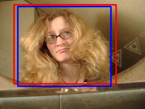
(a) DINO CLS Token Attention	(b) DINO Detection	(c) LOST Inverse Degree Attention	(d) LOST Detection	(e) Our Eigen Attention	(f) Our Detection

Figure 3: Visual results of unsupervised single object discovery on VOC12. In (a), we show the attention of the CLS token in DINO [6] which is used for detection (b). LOST [45] is mainly relied on the map of inverse degrees (c) to perform detection (d). For our approach, we illustrate the eigenvector in (e) and our detection in (f). Blue and Red bounding boxes indicate the ground-truth and the predicted bounding boxes respectively.

3.1.2 Normalized Cut (Ncut)

Graph partitioning.

Ncut [43] can be used to partition a graph into two disjoint sets A and B. The method partitions the graph so as to minimizing the Ncut energy [43]:

$$Ncut(A,B)=\frac{C(A,B)}{C(A,\mathcal{V})}+\frac{C(A,B)}{C(B,\mathcal{V})}$$ (1)

where $C$ measures the degree of similarity between two sets. $C(A,B)=\sum_{v_{i}\in A,v_{j}\in B}\mathcal{E}_{i,j}$ and $C(A,\mathcal{V})$ is the total connection from nodes in A to all nodes in the graph.

As shown by Shi and Malik [43], the optimization problem in Eqn 1 is equivalent to:

$$min_{\mathbf{x}}Ncut(\mathbf{x})=min_{\mathbf{y}}\frac{\mathbf{y}^{T}(\mathcal{D}-\mathcal{E})\mathbf{y}}{\mathbf{y}^{T}\mathcal{D}\mathbf{y}}.$$ (2)

With the condition $\mathbf{y}\in\{1,-b\}^{N}$, b satisfies $\mathbf{y}^{T}\mathcal{D}\mathbf{1}=0$. $\mathcal{D}$ is a diagonal matrix with $\mathbf{d}_{i}=\sum_{j}\mathcal{E}_{i,j}$ on its diagonal.

Ncut solution with the relaxed constraint.

Taking $\mathbf{z}=\mathcal{D}^{\frac{1}{2}}\mathbf{y}$. Eqn 2 can be rewrite as:

$$min_{\mathbf{z}}\frac{\mathbf{z}^{T}\mathcal{D}^{-\frac{1}{2}}(\mathcal{D}-\mathcal{E})\mathcal{D}^{-\frac{1}{2}}\mathbf{z}}{\mathbf{z}^{T}\mathbf{z}}.$$ (3)

Indicating in [43], the formulation in Eqn 3 is equivalent to the Rayleigh quotient [52], which is equivalent to solve $\mathcal{D}^{-\frac{1}{2}}(\mathcal{D}-\mathcal{E})\mathcal{D}^{-\frac{1}{2}}\mathbf{z}=\lambda\mathbf{z}$, where $\mathcal{D}-\mathcal{E}$ is the Laplacian matrix and known to be positive semidefinite [38]. Therefore $\mathbf{z}_{0}=\mathcal{D}^{\frac{1}{2}}\mathbf{1}$ is an eigenvector associated to the smallest eigenvalue $\lambda=0$. According to Rayleigh quotient [52], the second smallest eigenvector $\mathbf{z}_{1}$ is perpendicular to the smallest one ($\mathbf{z}_{0}$) and can be used to minimize the energy in Eqn 3,

$$\mathbf{z}_{1}=argmin_{\mathbf{z}^{T}\mathbf{z}_{0}}\frac{\mathbf{z}^{T}\mathcal{D}^{-\frac{1}{2}}(\mathcal{D}-\mathcal{E})\mathcal{D}^{-\frac{1}{2}}\mathbf{z}}{\mathbf{z}^{T}\mathbf{z}}.$$

Taking $\mathbf{z}=\mathcal{D}^{\frac{1}{2}}\mathbf{y}$,

$$\mathbf{y}_{1}=argmin_{\mathbf{y}^{T}\mathcal{D}\mathbf{1}=0}\frac{\mathbf{y}^{T}(\mathcal{D}-\mathcal{E})\mathbf{y}}{\mathbf{y}^{T}\mathcal{D}\mathbf{y}}.$$

Thus, the second smallest eigenvector of the generalized eigensystem $(\mathcal{D}-\mathcal{E})\mathbf{y}=\lambda\mathcal{D}\mathbf{y}$ is the real valued solution to the Ncut [43] problem.

3.2 TokenCut Algorithm

Graph construction.

Our method uses the vision transformers as described in Section 3.1.1 to produce a vector of features for each $K\times K$ image patch. A fully connected undirected graph $\mathcal{G}$ = ($\mathcal{V}$, $\mathcal{E}$) of patches is constructed where each $\mathcal{V}$ represents a patch with a feature vector $\{v_{i}\}_{i=1}^{N}$, and each patch is linked to adjacent patches by labeled edges, $\mathcal{E}$. Edge labels represent a similarity score $S$ based on the cosine similarity of the feature vectors of the two patches.

$$\mathcal{E}_{i,j}=\begin{cases}1,&\mbox{if }S(v_{i},v_{j})\geq\tau\\ \epsilon,&\mbox{else}\end{cases},$$ (4)

where $\tau$ is a hyper-parameter and $\epsilon$ equals a small value $1e-5$ to assure that the graph is fully connected and $S$ is the cosine similarity between features. Note that the spatial information has been implicitly included in the features via positional encoding in transformer.

$$S(v_{i},v_{j})=\frac{v_{i}v_{j}}{\lVert v_{i}\rVert_{2}\lVert v_{j}\rVert_{2}}.$$ (5)

We apply Ncut algorithm, as described in Section 3.1.2, on constructed graph $\mathcal{G}$ and obtain the second smallest eigenvector of the generalized eigensystem, which can be seen as an attention map of the potential objects. We provide visualization of this attention map in Section 4.

Discovering Salient Object with TokenCut.

We assume that there is at least one object in the image and the object occupies the foreground region. To successfully segment the foreground objects from the image, we must solve three problems: i) We must determine a means to partition the graph into two subgraphs and ii) given a bi-partition of the graph, we must determine which partition represents the foreground. iii) In case of detecting multiple connected components in the foreground, we must identify the most salient object.

For the first problem, in our initial experiments we have used a simple average value of the projection onto the second smallest eigenvector to determine the similarity value for cutting the graph $\overline{\mathbf{y}_{1}}=\frac{1}{N}\sum_{i}\mathbf{y}^{i}_{1}$. Formally, $A=\{v_{i}|\mathbf{y}^{i}_{1}\leq\overline{\mathbf{y}_{1}}\}$ and $B=\{v_{i}|\mathbf{y}^{i}_{1}>\overline{\mathbf{y}_{1}}\}$. We have compared this to using the classical clustering algorithms of K-means and EM to cluster the second smallest eigen vector into 2 partitions. The comparison is available in the supplementary material Table 6, indicating that the mean generally provides better results.

For the second problem, the foreground contains the salient object and is assumed to be less connected to the entire graph. Intuitively, $\mathbf{d}_{i}<\mathbf{d}_{j}$ if $v_{i}$ belongs to the foreground while $v_{j}$ is the background token. Therefore, the eigenvector of the foreground object should have a larger absolute value than the one of the background. We use the maximum absolute value $v_{max}$ to select the foreground partition and the most salient object. The partition that contains $v_{max}$ is taken as foreground. As our graph has no explicit spatial constraint, the foreground might contain more than one connected regions. We simply select the largest connected component existing in the foreground containing the maximum absolute value $v_{max}$ as our final object region.

Table 1: Comparisons for unsupervised single object discovery. We compare TokenCut to state-of-the-art object discovery methods on VOC07 [19], VOC12  [20] and COCO20K [33, 56] datasets. Model performances are evaluated with CorLoc metric. “Inter-image Simi.” means the model leverages information from the entire dataset and explores inter-image similarities to localize objects.

Method	Inter-image Simi.	DINO [6] Feat.	VOC07 [19]	VOC12  [20]	COCO20K [33, 56]
Selective Search [51, 45]	✗	-	18.8	20.9	16.0
EdgeBoxes [79, 45]	✗	-	31.1	31.6	28.8
Kim et al. [30, 45]	✓	-	43.9	46.4	35.1
Zhange et al. [74, 45]	✓	-	46.2	50.5	34.8
DDT+ [61, 45]	✓	-	50.2	53.1	38.2
rOSD [56, 45]	✓	-	54.5	55.3	48.5
LOD [57, 45]	✓	-	53.6	55.1	48.5
DINO-seg [6, 45]	✗	ViT-S/16 [18]	45.8	46.2	42.1
LOST [45]	✗	ViT-S/16 [18]	61.9	64.0	50.7
TokenCut	✗	ViT-S/16 [18]	68.8 ($\uparrow$ 6.9)	72.1 ($\uparrow$ 8.1)	58.8 ($\uparrow$ 8.1)
LOD + CAD⋆ [45]	✓	-	56.3	61.6	52.7
rOSD + CAD⋆ [45]	✓	-	58.3	62.3	53.0
LOST + CAD⋆ [45]	✗	ViT-S/16 [18]	65.7	70.4	57.5
TokenCut + CAD⋆ [45]	✗	ViT-S/16 [18]	71.4 ($\uparrow$ 5.7)	75.3 ($\uparrow$ 4.9)	62.6 ($\uparrow$ 5.1)

^⋆ +CAD indicates to train a second stage class-agnostic detector with “pseudo-boxes” labels.

In summary, the TokenCut algorithm consists of the following steps:

1. Given an image, build a graph $\mathcal{G}$ = ($\mathcal{V}$, $\mathcal{E}$) according to Equation 4 and 5.

2. Solve the generalized eigensystem $(\mathcal{D}-\mathcal{E})\mathbf{y}=\lambda\mathcal{D}\mathbf{y}$ for the eigenvector associated to the second smallest eigenvalue $\mathbf{y}_{1}$.

3. Compute bi-partition using the average over $\mathbf{y}_{1}$: $\overline{\mathbf{y}_{1}}=\sum_{i}\frac{\mathbf{y}^{i}_{1}}{N}$. $A=\{v_{i}|\mathbf{y}^{i}_{1}\leq\overline{\mathbf{y}_{1}}\}$ and $B=\{v_{i}|\mathbf{y}^{i}_{1}>\overline{\mathbf{y}_{1}}\}$

4. Find the largest connected component associated to the maximum absolute value of $\mathbf{y}_{1}$.

Implementation details.

For our experiments, we use the ViT-S/16 model [18] trained with self-distillation loss (DINO) [6] to extract features of patches. We employ the keys features of the last layer as the input features $v$. Ablations on different features as well as transformers trained with self-supervised learning are provided in the supplementary material Table  5. We set $\tau=0.2$ for all datasets, the dependency on $\tau$ is provided in Section 4.4. In terms of running time, our un-optimised implementation takes approximately 0.32 seconds to detect a bounding box of a single image with resolution 480 $\times$ 480 on a single GPU QUADRO RTX 8000.

4 Experiments

We evaluate our approach on three tasks: unsupervised single object discovery, weakly supervised object detection and unsupervised saliency detection. We present results of unsupervised single object discovery in Section 4.1. The results of weakly supervised object detection are in Section 4.2. The results of unsupervised saliency detection in Section 4.3. We provide analysis of $\tau$ in Section 4.4, other ablation studies will be presented in supplementary material.

4.1 Unsupervised Single Object Discovery

Evaluation metric.

We report performance using the CorLoc metric for precise localisation, as used by  [15, 56, 57, 55, 61, 11, 47]. CorLoc counts a predicted bounding box as correct if the intersection over union (IoU) score between the predicted bounding box and one of the ground truth bounding boxes is superior to 0.5.

Table 2: Comparisons for weakly supervised object localization. We report Top-1 Cls, GT Loc and Top-1 Loc on CUB [59] and ImageNet-1K [14] datasets. Compared state-of-the-art methods are divided into two groups: with ImageNet-1K supervised pretraining and with ImageNet-1K self-supervised pretraining.

Pretrained Dataset	Method	Backbone	CUB [59], Acc. (%)			ImageNet-1K [14], Acc. (%)
			Top-1 Cls	GT Loc	Top-1 Loc	Top-1 Cls	GT Loc	Top-1 Loc
ImageNet-1K [14] supervised pretrain	CAM [77]	GoogLeNet [48]	73.8	-	41.1	65	-	43.6
	HaS-32 [46] + [3]	GoogLeNet [48]	75.4	61.1	47.4	68.9	60.6	44.6
	ADL [13] + [3]	ResNet50 [24]	75.0	77.6	59.5	75.8	62.2	49.4
	ADL [13]	InceptionV3 [49]	74.6	-	53.0	72.8	-	48.7
	I2C [76]	InceptionV3 [49]	-	72.6	56	73.3	68.5	53.1
	PSOL [71]‡	InceptionV3 [49]	-	-	65.5	-	65.2	54.8
	SLT-Net [22]⋆	InceptionV3 [49]	76.4	86.5	66.1	78.1	67.6	55.7
ImageNet-1K [14] self-supervised pretrain	LOST [45]	ViT-S/16 [18]	79.5	89.7	71.3	77.0	60.0	49
	TokenCut	ViT-S/16 [18]	79.5	91.8 ($\uparrow$ 2.1)	72.9 ($\uparrow$ 1.6)	77.0	65.4 ($\uparrow$ 5.4)	52.3 ($\uparrow$ 3.3)

$\star$ uses ten crop augmentations to get final classification results. $\star$ and $\ddagger$ learn a classifer and a detector separately.

Table 3: Comparisons for unsupervised saliency detection We compare TokenCut to state-of-the-art unsupervised saliency detection methods on ECSSD [44], DUTS [60] and DUT-OMRON [67]. TokenCut achieves better results comparing with other competitive approaches.

Method	ECSSD [44]			DUTS [60]			DUT-OMRON [67]
	$maxF_{\beta}$(%)	IoU(%)	Acc.(%)	$maxF_{\beta}$(%)	IoU(%)	Acc.(%)	$maxF_{\beta}$(%)	IoU(%)	Acc.(%)
HS [66]	67.3	50.8	84.7	50.4	36.9	82.6	56.1	43.3	84.3
wCtr [78]	68.4	51.7	86.2	52.2	39.2	83.5	54.1	41.6	83.8
WSC [31]	68.3	49.8	85.2	52.8	38.4	86.2	52.3	38.7	86.5
DeepUSPS [37]	58.4	44.0	79.5	42.5	30.5	77.3	41.4	30.5	77.9
BigBiGAN [58]	78.2	67.2	89.9	60.8	49.8	87.8	54.9	45.3	85.6
E-BigBiGAN [58]	79.7	68.4	90.6	62.4	51.1	88.2	56.3	46.4	86.0
LOST [45, 42]	75.8	65.4	89.5	61.1	51.8	87.1	47.3	41.0	79.7
LOST [45, 42]+Bilateral Solver [5]	83.7	72.3	91.6	69.7	57.2	88.7	57.8	48.9	81.8
TokenCut	80.3	71.2	91.8	67.2	57.6	90.3	60.0	53.3	88.0
TokenCut + Bilateral Solver [5]	87.4 ($\uparrow$ 3.7)	77.2($\uparrow$ 4.9)	93.4 ($\uparrow$ 1.8)	75.5($\uparrow$ 5.8)	62.4 ($\uparrow$ 5.2)	91.4 ($\uparrow$ 2.7)	69.7 ($\uparrow$ 11.9)	61.8 ($\uparrow$ 12.9)	89.7 ($\uparrow$ 7.9)

Quantitative Results.

We evaluate our approach on three commonly used benchmarks for unsupervised single object discovery: VOC07 [19] , VOC12 [20] and COCO20K  [33, 56]. The qualitative results are provided in Tab. 1. We evaluate the CorLoc scores in comparison with previous state-of-the-art single object discovery methods [51, 79, 45, 30, 74, 61, 56, 57] on VOC07, VOC12, and COCO20K datasets. These methods can be roughly divided into two groups based on whether the model leverages information from the entire dataset and explores inter-image similarities or not. Because of quadratic complexity of region comparison among images, models with inter-image similarities are generally difficult to scale to larger datasets. The selective search [51], edge boxes [79], LOST [45] and TokenCut do not require inter-image similarities and are thus much more efficient. As shown in the table, TokenCut consistently outperforms all previous methods on all datasets by a large margin. Specifically, TokenCut improves the state-of-the-art by 6.9%, 8.1% and 8.1% in VOC07, VOC12 and COCO20K respectively using the same ViT-S/16 features.

We also list a set of results that including a second stage unsupervised training strategy to boost the performance, This is referred to as class-agnostic detection (CAD). A CAD is trained by assigning the same “foreground” category to all the boxes produced by the first stage single object discovery model. As shown in Tab. 1, TokenCut + CAD outperforms the state-of-the-art by 5.7%, 4.9% and 5.1% on VOC07, VOC12 and COCO20k respectively.

Qualitative Results.

In Fig. 3, we provide visualization for DINO-seg [6], LOST [45] and Tokencut. For each method, we visualize the heatmap that is used to perform object detection. For DINO-seg, the heatmap is the attention map associated to the CLS token. For LOST, the detection is mainly based on the map of inverse degree ($\frac{1}{\mathbf{d}_{i}}$). For TokenCut, we display the second smallest eigenvector. The visual result demonstrates that Tokencut can extract a high quality segmentation of the salient object. Comparing with DINO-seg and LOST, TokenCut is able to extract a more complete segmentation as can be seen in the first and the third samples in Fig. 3. In some other cases, when all the methods have a high quality map, TokenCut has the strongest intensity on the object, this phenomenon can be viewed in the last sample in Fig. 3. More visual results can be found in the supplementary material Fig. 7 and Fig. D.

4.2 Weakly Supervised Object Localization

Evaluation metrics.

We report three standard metrics: Top-1 Cls, GT Loc and Top-1 Loc. Top-1 Cls represents the top-1 accuracy of image classification. GT Loc is similar to CorLoc in which a predicted box is counted as correct if the IoU score is superior to 0.5 between the predicted bounding box and one of the ground-truth bounding boxes. Top-1 Loc is the most important metric as it considers measuring both the classification and the detection: a predicted bounding box is counted as a true positive if the class of the image is correctly predicted and the IoU is superior to 0.5 between the predicted bounding box and the ground-truth bounding box.

Results.

We use two datasets to evaluate model performances on weakly supervised object localization: CUB-200-2011 [59] (CUB) and ImangeNet-1k [40]. The fine-tuning details can be found in supplementary material. In Tab. 2, we compare TokenCut to the state-of-the-art weakly-supervised object localization approaches on CUB and ImageNet-1K datasets. The methods can be divided to two groups: models initialized with ImageNet-1K supervised pre-training [77, 46, 13, 76, 71, 22, 3] and models inilialized with ImageNet-1K self-supervised pre-training [45].

On the CUB dataset, TokenCut achieves the best performance over all methods, and outperforms the state-of-the-art LOST method by 2.1% and 1.6% on GT Loc and Top-1 Loc. Interestingly, all the ImageNet-1K self-supervised pretraining models are better than the supervised pretrained models. We believe that this is because supervised pretraining learns a more discriminative representation of the pretrained dataset than self-supervised pretraining, leading to a reduction in transferability to downstream datasets such as CUB. In comparison, self-supervised pretraining can learn a more general represenatation and thus provides better transferbility.

On the ImageNet-1K dataset, TokenCut outperforms LOST by 5.4% and 4.4% on GT Loc and Top-1 Loc, and achieves a comparable performance with the ImageNet-1K supervised pretrain model. If the downstream task is ImageNet-1K, then the supervised pretraining with ImageNet-1K can provide discriminative features that improve the localization task as they are tuned to the dataset.

Table 4: Analysis of $\tau$. We report CorLoc for unsupervised single object discovery on VOC07, VOC12, COCO20K, and Top-1 Loc for weakly supervised object detection on CUB and ImageNet-1K.

$\tau$	CorLoc			Top-1 Loc
	VOC07	VOC12	COCO20K	CUB	ImageNet-1K
0	67.4	71.3	56.1	73.0	53.8
0.1	68.6	72.1	58.2	73.2	53.4
0.2	68.8	72.1	58.8	72.9	52.3
0.3	67.7	72.1	58.2	70.8	50.4

4.3 Unsupervised Saliency detection

(a) Input	(b) Ours	(c) Ours + BS	(d) GT

Figure 4: Visual results of unsupervised segments on ECSSD [44]. In (a), we show the input image. TokenCut detection result is presented in (b). TokenCut + Bilateral Solver results is shown in (c). (d) is the ground truth.

Evaluation Metrics

We report three standard metrics: F-measure, IoU and Accuracy. F-measure is a standard measure in saliency detection. It is computed as $F_{\beta}=\frac{(1+\beta^{2})Precision\times Recall}{\beta^{2}Precision+Recall}$, where the Precision and Recall are defined based on the binarized predicted mask and ground truth mask. The $maxF_{\beta}$ is the maximum value of 255 uniformly distributed binarization thresholds. Following previous works [42, 58], we set $\beta=0.3$ for consistency. IoU(Intersection over Union) score is computed based on the binary predicted mask and the ground-truth, the threshold is set to 0.5. Accuracy measures the proportion of pixels that have been correctly assigned to the object/background. The binarization threshold is set to 0.5 for masks.

Results

We further evaluate TokenCut on three commonly datasets for unsupervised saliency detection: ECSSD [44], DUTS [60] and DUT-OMRON [67]. The qualitative results are in Tab. 3. TokenCut significantly outperforms previous state-of-the-art. Adding Bilateral Solver [5] refines the boundary of an object and further boosts the performance over TokenCut, which can also be seen from the visual results presented in Fig. 4.

(a) Input	(b) Eigen Attention	(c) Detection

Figure 5: Visual results of images taken from the Internet. We show the input images, our eigen attention and final detection in (a) (b) (c) respectively.

4.4 Analysis and Discussion

Analysis of $\tau$.

In Tab. 4, we provide an analysis on $\tau$ defined in Equation 4. The results indicate that the effects of variations in $\tau$ value are not significant and that a suitable threshold is $\tau$ = 0.2.

Internet Images

We further test TokenCut  on Internet images. The results are in Figure 5. We can see even the inputs images are with noisy background, our algorithm can still provide precise attention map cover the object leading to accurate bounding box prediction, which demonstrates again the robustness of our approach.

Limitations

Despite the good performance of TokenCut, it has several limitations. Examples of failure cases are shown in Fig. 6: i) TokenCut focuses on the largest salient part in the image, which may not be the desired object (Fig. 6, 1st row). ii) Similar to LOST [45], TokenCut assumes that a single salient object occupies the foreground. If multiple overlapping objects are present in an image, both LOST and our approach will fail to detect one of the object (Fig. 6, 2nd row). iii) Neither LOST nor our approach can handle occlusion (Fig. 6, 3rd row).

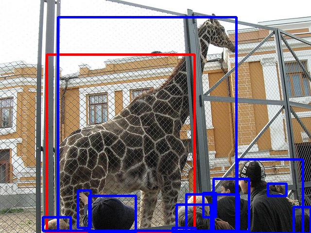
(a) LOST Inverse Attn.	(b) LOST Detection	(c) Our Eigen Attention	(d) Our Detection

Figure 6: Failure cases on VOC12 (1st and 2nd row) and COCO (3rd row). LOST [45] mainly relies on the map of inverse degrees (a) to perform detection (b). For our approach, we illustrate the eigenvector in (c) and our detection in (d). Blue and Red bounding boxes indicate the ground-truth and the predicted bounding boxes respectively.

5 Conclusion

We have introduced TokenCut, a simple but effective approach for unsupervised object discovery. TokenCut uses self-supervised learning with transformers to constructs a graph where nodes are patches and edges represent similarities between patches. We showed that salient objects can be directly detected and delimited using Ncut. We evaluated this approach on unsupervised single object discovery, weakly supervised object detection and unsupervised saliency detection, and showed that it provides a significant improvement over previous approaches. Our results indicate that self-supervised transformers can provide a rich and general set of features that may likely be used for a variety of computer vision problems.

Acknowledgements This work has been partially supported by the MIAI Multidisciplinary AI Institute at the Univ. Grenoble Alpes (MIAI@Grenoble Alpes - ANR-19-P3IA-0003), and by the EU H2020 ICT48 project Humane AI Net under contract EU #952026.

Appendix A Analysis of backbones.

In Tab. 5, we provide an ablation study on different transformer backbones. The “-S” and “-B” are ViT small[18, 6] and ViT base[18, 6] architecture respectively. The “-16” and “-8” represents patch sizes 16 and 8 respectively. The “MocoV3” is another pre-trained self-supervised transformer model [8]. The $\tau$ value is set to 0.3 for MoCov3, while for Dino the best tau value is 0.2. We observe that although the result of MoCov3 is slightly worse than the results of TokenCut with Dino, MoCov3 still outperforms previous state-of-the-art, indicating that TokenCut can provide similar results when used with other self-supervised Transformer architectures. Besides, the results demonstrates that a patch size of 16 provides better results than a patch size of 8. Several insights can be found: i) TokenCut outperforms LOST for different backbones. ii) As LOST relies on a heuristic seeds expansion strategy, the performance varies significantly using different backbones. While our approach is more robust.

Table 5: Analysis of different backbones. We report CorLoc for unsupervised single object discovery on VOC07, VOC12, COCO20K.

Method	Backbone	VOC07	VOC12	COCO20K
LOST [45]	ViT-S/16 [18, 6]	61.9	64.0	50.7
TokenCut	MoCoV3-ViT-S/16 [18, 8]	66.2	66.9	54.5
TokenCut	ViT-S/16 [18, 6]	68.8 ($\uparrow$ 6.9)	72.1 ($\uparrow$ 8.1)	58.8 ($\uparrow$ 8.1)
LOST [45]	ViT-S/8 [18, 6]	55.5	57.0	49.5
TokenCut	ViT-S/8 [18, 6]	67.3 ($\uparrow$ 11.8)	71.6 ($\uparrow$ 14.6)	60.7 ($\uparrow$ 11.2)
LOST [45]	ViT-B/16 [18, 6]	60.1	63.3	50.0
TokenCut	ViT-B/16 [18, 6]	68.8 ($\uparrow$ 8.7)	72.4 ($\uparrow$ 9.1)	59.0 ($\uparrow$ 9.0)

We provide another an ablation study on different backbones for weakly supervised object localization. Results are shown in Tab. A. The “-S” and “-B” designate ViT small [6, 18] and ViT base [6, 18] architecture respectively. The “-16” and “-8” indicate patch sizes 16 and 8 respectively. For our approach, we report results with $\tau=0.2$, which is the same on all the datasets. Note that LOST with ViT-S/8 achieves much worse results, because the seed expansion strategy in LOST relies on the top-100 patches which are with lowest degrees. When the total number of patches is large, the proposed seed expansion strategy is not able to cover entire objects. While our approach provides more robust performance on different datasets across different backbones.

+Analysis of backbones for weakly supervised object localization. We report Top-1 Cls, GT Loc and Top-1 Loc on CUB [59] and Imagenet-1k [14] datasets.

Method	Backbone	$\tau$	CUB [50], Acc. (%)			ImageNet-1K [11], Acc. (%)
			Top-1 Cls	GT Loc	Top-1 Loc	Top-1 Cls	GT Loc	Top-1 Loc
LOST [45]	ViT-S/16 [18, 6]	-	79.5	89.7	71.3	77.0	60.0	49.0
TokenCut	ViT-S/16 [18, 6]	0.2	79.5	91.8 ($\uparrow$ 2.1)	72.9 ($\uparrow$ 1.6)	77.0	65.4 ($\uparrow$ 5.4)	53.4 ($\uparrow$ 4.4)
LOST [45]	ViT-S/8 [18, 6]	-	82.3	78.0	64.4	79.4	45.8	38.1
TokenCut	ViT-S/8 [18, 6]	0.2	82.3	89.9 ($\uparrow$ 11.9)	74.2 ($\uparrow$ 9.8)	79.4	66.0 ($\uparrow$ 20.2)	55.0 ($\uparrow$ 16.9)
LOST [45]	ViT-B/16 [18, 6]	-	80.3	90.7	72.8	78.3	58.6	48.3
TokenCut	ViT-B/16 [18, 6]	0.2	80.3	90.0 ($\downarrow$ 0.7)	72.5 ($\downarrow$ 0.3)	78.3	63.2 ($\uparrow$ 4.8)	52.3 ($\uparrow$ 4.0)

Appendix B Analysis of bi-partition strategies.

In Tab. 6, we study different strategies to separate the nodes in our graph into two groups using the second smallest eigenvector. We consider three natural methods: mean value (Mean), Expectation-Maximisation (EM), K-means clustering (K-means). We use python sklearn library for EM and K-means algorithm implementation. For EM algorithm, we set number of iteration to 300 and each component has its own general covariance matrix. The convergence threshold is set to 1e-3. For K-means algorithm, we use “k-means++” for initialization. The maximum number of iterations is set to 300. The convergence threshold is set to 1e-4. The result suggests that the simple mean value as the splitting point performs well for most cases. We have also tried to search for the splitting point based on the best Ncut(A,B) value. Due to the quadratic complexity, this approach requires substantially more computations. Thus, we finally obsolete it.

Table 6: Analysis of different bi-partition methods. We report CorLoc for unsupervised single object discovery.

Bi-partition	VOC07	VOC12	COCO20K
Mean	68.8	72.1	58.8
EM	63.0	65.7	59.3
K-means	67.5	69.2	61.6

Appendix C Analysis of Graph edge weight

In this section, we provide an ablation study on graph edge weight defininig on equation 4. We have tested to directly use the similarity score as edge weights (i.e., $\mathcal{E}_{ij}=S(x_{i},x_{j}))$). However, it is not possible because there may exist negative edge values, which violates the Normalized Cut algorithm assumption. Thus, we also tried thresholding the similarity score (i.e., $\mathcal{E}_{ij}=S(x_{i},x_{j})$ if $S(x_{i},x_{j})>\tau$, else $\epsilon$). We obtain 68.9% on VOC07 dataset and 72% on VOC12 dataset, which is similar to our reported results.

Appendix D Visual results for unsupervised single object discovery on VOC07 and COCO12

We show visual results for unsupervised single object discovery on VOC07 [19] and COCO12 [33, 56], which are illustrated in Fig. 7 and Fig. D respectively.

For each dataset, we compare both attention maps and bounding box predictions among DINO [6], LOST [45] and TokenCut. The attention map for DINO is extracted from the CLS token attention map of the last layer of key features. The attention map for LOST is the inverse degree map used in LOST for detection. The TokenCut attention map is the second smallest eigenvector of Equation 2. These results show that TokenCut provides clearly better segmentation of the object.

(a) DINO CLS Token Attention	(b) DINO Detection	(c) LOST Inverse Degree Attention	(d) LOST Detection	(e) Our Eigen Attention	(f) Our Detection

Figure 7: Visual results of unsupervised single object discovery on VOC07 [19] In (a), we show the attention of the CLS token in DINO [6] which is used for detection (b). LOST [45] is mainly relied on the map of inverse degrees (c) to perform detection (d). For our approach, we illustrate the eigenvector in (e) and our detection in (f). Blue and Red bounding boxes indicate the ground-truth and the predicted bounding boxes respectively.

(a) DINO CLS Token Attention	(b) DINO Detection	(c) LOST Inverse Degree Attention	(d) LOST Detection	(e) Our Eigen Attention	(f) Our Detection

+Visual results of unsupervised single object discovery on COCO20K [33, 56]. In (a), we show the attention of the CLS token in DINO [6] used for detection (b). LOST [45] mainly relies on the map of inverse degrees (c) to perform detection (d). For TokenCut, we illustrate the eigenvector in (e) and the detection in (f). Blue and Red bounding boxes indicate the ground-truth and the predicted bounding boxes respectively.

Appendix E Fine-tuning self-supervised transformers

For weakly supervised object localization, we use a pre-trained DINO model as our backbone and learn a linear classifier on the training set where we only have access to the class labels. We freeze the backbone weights and fine-tune a linear classifier, as shown in Tab. 2. For CUB, We train with a SGD optimizer for 1000 epochs and set the batch size to 256 per GPU, distributed over 4 GPUs. The learning rate is linearly warmed during the first 50 epochs, then follows a cosine learning rate scheduler. We decay the learning rate from $\frac{\text{batch\leavevmode\nobreak\ size}}{256}\times$5e-4 to 1e-6. The weight decay is set to 0.005. For ImageNet-1K, we use the models released by DINO. Other training setups and details can be found in the supplementary material.

Appendix F Visual results for weakly supervised object localizatio on CUB and Imagenet-1k

We present visual results for weakly supervised object localization on CUB [59] and Imagenet-1k [14] in Fig. F and Fig. F respectively.

For each dataset, we compare the attention map and bounding box prediction with LOST [45] and our approach. The eigenvector of TokenCut provides better segmentation on objects and leads to better detection results.

(a) LOST Inverse Degree Attention
(b) LOST Detection
(c) Ours Eigen Attention
(d) Ours Detection

Visual results for weakly supervised object localization on CUB [59]. In (a), we show the map of inverse degrees used to perform detection with LOST (b) [45]. For TokenCut, we illustrate the eigenvector in (c) used for detection in (d). Blue and Red bounding boxes indicate the ground-truth and the predicted bounding boxes respectively.

(a) LOST Inverse Degree Attention
(b) LOST Detection
(c) Ours Eigen Attention
(d) Ours Detection

+Visual results of unsupervised single object discovery on Imagenet-1k [14]. In (a), we show LOST  [45] the map of inverse degrees, which is used to perform detection (b). For TokenCut, we illustrate the eigenvector in (c) and the detection in (d). Blue and Red bounding boxes indicate the ground-truth and the predicted bounding boxes respectively.

Appendix G Failure cases on CUB and Imagenet-1k

We illustrate additional failure cases in Fig. G. Those failure cases can be organised into three categories: 1) Where TokenCut focus on the largest salient object, whereas the annotation is highlights a different object, shown in the first and the second column in Fig. G. 2) Similar to LOST, Tokencut is not able to differentiate the connected objects, such as the third and the fourth column in Fig. G. 3) In case of occlusion, neither LOST nor our approach can’t detect the entire object, such as the last two columns in Fig. G.

(a) LOST Inverse Degree Attention
(b) LOST Detection
(c) Ours Eigen Attention
(d) Ours Detection

+Failure cases on Imagenet-1k [14] and CUB [59]. In (a), we show LOST [45] the map of inverse degrees, which is used to perform detection (b). For TokenCut, we illustrate the eigenvector in (c) and the detection in (d). Blue and Red bounding boxes indicate the ground-truth and the predicted bounding boxes respectively.

Appendix H Datasets

We present in this section the details of the datasets used in our experiments:

• VOC07 and VOC12 correspond to the training and validation set of PASCAL-VOC07 and PASCAL-VOC12. VOC07 and VOC12 contain 5 011 and 11 540 images respectively which belong to 20 categories. They are commonly evaluated for unsupervised object discovery [56, 57, 55, 61, 11].

• COCO20K consists of 19 817 randomly chosen images from the COCO2014 dataset [33]. It is used as a benchmark in [56] for a large scale evaluation.

• CUB consists of 200 bird species, including 6 033 and 5 755 images in training and test sets respectively, which is commonly used to evaluate weakly supervised object localization [77, 46, 3, 48, 13].

• ImageNet [14] is a widely used benchmark for image classification and object detection, which consists of 1 000 different categories. The number of images in training and validation sets are 1.3 million and 50,000 respectively. Each image contains a single object supposed to be detected. During the training, only class labels are available.

• ECSSD contains 1 000 real-world images of complex scenes for testing.

• DUTS contains 10 553 train and 5 019 test images. The training set is collected from the ImageNet detection train/val set. The test set is collected from ImageNet test, and the SUN dataset [65]. Following the previous works [42], we report the performance on the DUTS-test subset.

• DUT-OMRON [67] contains 5 168 images of high quality natural images for testing.

Appendix I Visual results for unsupervised saliency detecion on ECSSD, DUTS and DUT-OMRON

We present visual results for unsupervised saliency detecion on ECSSD [44], DUTS [60] and DUT-OMRON [67] in Fig. 8, 9 and 10 respectively.

For each dataset, we compare LOST segmentation, LOST + Bilateral Solver and our approch. The TokenCut provides better segmentation on objects. The performance is further improved with Bilateral Solver.

(a) Input	(b) LOST	(c) LOST + BS	(d) Ours	(e) Ours + BS	(f) GT

Figure 8: Visual results of unsupervised segments on ECSSD [44]

(a) Input	(b) LOST	(c) LOST + BS	(d) Ours	(e) Ours + BS	(f) GT

Figure 9: Visual results of unsupervised segments on DUTS [60]

(a) Input	(b) LOST	(c) LOST + BS	(d) Ours	(e) Ours + BS	(f) GT

Figure 10: Visual results of unsupervised segments on DUT-OMRON [67]

References

- [1] Hamed H Aghdam, Abel Gonzalez-Garcia, Joost van de Weijer, and Antonio M López. Active learning for deep detection neural networks. In ICCV, 2019.
- [2] Jimmy Lei Ba, Jamie Ryan Kiros, and Geoffrey E Hinton. Layer normalization. arXiv, 2016.
- [3] Wonho Bae, Junhyug Noh, and Gunhee Kim. Rethinking class activation mapping for weakly supervised object localization. In ECCV, 2020.
- [4] Hangbo Bao, Li Dong, and Furu Wei. Beit: Bert pre-training of image transformers. arXiv, 2021.
- [5] Jonathan T Barron and Ben Poole. The fast bilateral solver. In ECCV, 2016.
- [6] Mathilde Caron, Hugo Touvron, Ishan Misra, Hervé Jégou, Julien Mairal, Piotr Bojanowski, and Armand Joulin. Emerging properties in self-supervised vision transformers. In ICCV, 2021.
- [7] Aditya Chattopadhay, Anirban Sarkar, Prantik Howlader, and Vineeth N Balasubramanian. Grad-cam++: Generalized gradient-based visual explanations for deep convolutional networks. In WACV, 2018.
- [8] Xinlei Chen, Saining Xie, and Kaiming He. An empirical study of training self-supervised vision transformers. In ICCV, 2021.
- [9] Yun-Chun Chen, Yen-Yu Lin, Ming-Hsuan Yang, and Jia-Bin Huang. Show, match and segment: Joint weakly supervised learning of semantic matching and object co-segmentation. PAMI, 2020.
- [10] Ming-Ming Cheng, Niloy J Mitra, Xiaolei Huang, Philip HS Torr, and Shi-Min Hu. Global contrast based salient region detection. TPAMI, 2014.
- [11] Minsu Cho, Suha Kwak, Cordelia Schmid, and Jean Ponce. Unsupervised object discovery and localization in the wild: Part-based matching with bottom-up region proposals. In CVPR, 2015.
- [12] Junsuk Choe, Seong Joon Oh, Seungho Lee, Sanghyuk Chun, Zeynep Akata, and Hyunjung Shim. Evaluating weakly supervised object localization methods right. In CVPR, 2020.
- [13] Junsuk Choe and Hyunjung Shim. Attention-based dropout layer for weakly supervised object localization. In CVPR, 2019.
- [14] Jia Deng, Wei Dong, Richard Socher, Li-Jia Li, Kai Li, and Li Fei-Fei. Imagenet: A large-scale hierarchical image database. In CVPR, 2009.
- [15] Thomas Deselaers, Bogdan Alexe, and Vittorio Ferrari. Localizing objects while learning their appearance. In ECCV, 2010.
- [16] Jacob Devlin, Ming-Wei Chang, Kenton Lee, and Kristina Toutanova. Bert: Pre-training of deep bidirectional transformers for language understanding. In NAACL-HLT, 2018.
- [17] Terrance DeVries and Graham W Taylor. Improved regularization of convolutional neural networks with cutout. arXiv, 2017.
- [18] Alexey Dosovitskiy, Lucas Beyer, Alexander Kolesnikov, Dirk Weissenborn, Xiaohua Zhai, Thomas Unterthiner, Mostafa Dehghani, Matthias Minderer, Georg Heigold, Sylvain Gelly, et al. An image is worth 16x16 words: Transformers for image recognition at scale. In ICLR, 2020.
- [19] M. Everingham, L. Van Gool, C. K. I. Williams, J. Winn, and A. Zisserman. The PASCAL Visual Object Classes Challenge 2007 (VOC2007) Results. http://www.pascal-network.org/challenges/VOC/voc2007/workshop/index.html.
- [20] M. Everingham, L. Van Gool, C. K. I. Williams, J. Winn, and A. Zisserman. The PASCAL Visual Object Classes Challenge 2012 (VOC2012) Results. http://www.pascal-network.org/challenges/VOC/voc2012/workshop/index.html.
- [21] Andreas Geiger, Philip Lenz, Christoph Stiller, and Raquel Urtasun. Vision meets robotics: The kitti dataset. The International Journal of Robotics Research, 2013.
- [22] Guangyu Guo, Junwei Han, Fang Wan, and Dingwen Zhang. Strengthen learning tolerance for weakly supervised object localization. In CVPR, 2021.
- [23] Kaiming He, Xinlei Chen, Saining Xie, Yanghao Li, Piotr Dollár, and Ross Girshick. Masked autoencoders are scalable vision learners. arXiv, 2015.
- [24] Kaiming He, Xiangyu Zhang, Shaoqing Ren, and Jian Sun. Deep residual learning for image recognition. In CVPR, 2016.
- [25] Geoffrey Hinton, Oriol Vinyals, and Jeff Dean. Distilling the knowledge in a neural network. arXiv, 2015.
- [26] Kuang-Jui Hsu, Yen-Yu Lin, Yung-Yu Chuang, et al. Co-attention cnns for unsupervised object co-segmentation. In IJCAI, 2018.
- [27] Huaizu Jiang, Jingdong Wang, Zejian Yuan, Yang Wu, Nanning Zheng, and Shipeng Li. Salient object detection: A discriminative regional feature integration approach. In CVPR, 2013.
- [28] Armand Joulin, Francis Bach, and Jean Ponce. Discriminative clustering for image co-segmentation. In CVPR, 2010.
- [29] Armand Joulin, Francis Bach, and Jean Ponce. Multi-class cosegmentation. In CVPR, 2012.
- [30] Gunhee Kim and Antonio Torralba. Unsupervised detection of regions of interest using iterative link analysis. In NeurIPS, 2009.
- [31] Nianyi Li, Bilin Sun, and Jingyi Yu. A weighted sparse coding framework for saliency detection. In CVPR, 2015.
- [32] Zhaowen Li, Zhiyang Chen, Fan Yang, Wei Li, Yousong Zhu, Chaoyang Zhao, Rui Deng, Liwei Wu, Rui Zhao, Ming Tang, et al. Mst: Masked self-supervised transformer for visual representation. In NeurIPS, 2021.
- [33] Tsung-Yi Lin, Michael Maire, Serge Belongie, James Hays, Pietro Perona, Deva Ramanan, Piotr Dollár, and C Lawrence Zitnick. Microsoft coco: Common objects in context. In ECCV, 2014.
- [34] Yen-Cheng Liu, Chih-Yao Ma, Zijian He, Chia-Wen Kuo, Kan Chen, Peizhao Zhang, Bichen Wu, Zsolt Kira, and Peter Vajda. Unbiased teacher for semi-supervised object detection. In ICLR, 2021.
- [35] Weizeng Lu, Xi Jia, Weicheng Xie, Linlin Shen, Yicong Zhou, and Jinming Duan. Geometry constrained weakly supervised object localization. In ECCV, 2020.
- [36] Jinjie Mai, Meng Yang, and Wenfeng Luo. Erasing integrated learning: A simple yet effective approach for weakly supervised object localization. In CVPR, 2020.
- [37] Tam Nguyen, Maximilian Dax, Chaithanya Kumar Mummadi, Nhung Ngo, Thi Hoai Phuong Nguyen, Zhongyu Lou, and Thomas Brox. Deepusps: Deep robust unsupervised saliency prediction via self-supervision. In NeurIPS, 2019.
- [38] Alex Pothen, Horst D Simon, and Kang-Pu Liou. Partitioning sparse matrices with eigenvectors of graphs. SIAM journal on matrix analysis and applications, 1990.
- [39] Zhongzheng Ren, Zhiding Yu, Xiaodong Yang, Ming-Yu Liu, Yong Jae Lee, Alexander G Schwing, and Jan Kautz. Instance-aware, context-focused, and memory-efficient weakly supervised object detection. In CVPR, 2020.
- [40] Olga Russakovsky, Jia Deng, Hao Su, Jonathan Krause, Sanjeev Satheesh, Sean Ma, Zhiheng Huang, Andrej Karpathy, Aditya Khosla, Michael Bernstein, et al. Imagenet large scale visual recognition challenge. IJCV, 2015.
- [41] Ramprasaath R Selvaraju, Michael Cogswell, Abhishek Das, Ramakrishna Vedantam, Devi Parikh, and Dhruv Batra. Grad-cam: Visual explanations from deep networks via gradient-based localization. In ICCV, 2017.
- [42] Xi Shen, Alexei A Efros, Armand Joulin, and Mathieu Aubry. Learning co-segmentation by segment swapping for retrieval and discovery. arXiv preprint arXiv:2110.15904, 2021.
- [43] Jianbo Shi and Jitendra Malik. Normalized cuts and image segmentation. TPAMI, 2000.
- [44] Jianping Shi, Qiong Yan, Li Xu, and Jiaya Jia. Hierarchical image saliency detection on extended cssd. TPAMI, 2015.
- [45] Oriane Siméoni, Gilles Puy, Huy V. Vo, Simon Roburin, Spyros Gidaris, Andrei Bursuc, Patrick Pérez, Renaud Marlet, and Jean Ponce. Localizing objects with self-supervised transformers and no labels. In BMVC, 2021.
- [46] Krishna Kumar Singh and Yong Jae Lee. Hide-and-seek: Forcing a network to be meticulous for weakly-supervised object and action localization. In ICCV, 2017.
- [47] Parthipan Siva, Chris Russell, Tao Xiang, and Lourdes Agapito. Looking beyond the image: Unsupervised learning for object saliency and detection. In CVPR, 2013.
- [48] Christian Szegedy, Wei Liu, Yangqing Jia, Pierre Sermanet, Scott Reed, Dragomir Anguelov, Dumitru Erhan, Vincent Vanhoucke, and Andrew Rabinovich. Going deeper with convolutions. In CVPR, 2015.
- [49] Christian Szegedy, Vincent Vanhoucke, Sergey Ioffe, Jon Shlens, and Zbigniew Wojna. Rethinking the inception architecture for computer vision. In CVPR, 2016.
- [50] Kevin Tang, Armand Joulin, Li-Jia Li, and Li Fei-Fei. Co-localization in real-world images. In CVPR, 2014.
- [51] Jasper RR Uijlings, Koen EA Van De Sande, Theo Gevers, and Arnold WM Smeulders. Selective search for object recognition. IJCV, 2013.
- [52] Charles F Van Loan and G Golub. Matrix computations. The Johns Hopkins University Press, 1996.
- [53] Ashish Vaswani, Noam Shazeer, Niki Parmar, Jakob Uszkoreit, Llion Jones, Aidan N Gomez, Lukasz Kaiser, and Illia Polosukhin. Attention is all you need. In NeurIPS, 2017.
- [54] Sara Vicente, Carsten Rother, and Vladimir Kolmogorov. Object cosegmentation. In CVPR, 2011.
- [55] Huy V Vo, Francis Bach, Minsu Cho, Kai Han, Yann LeCun, Patrick Pérez, and Jean Ponce. Unsupervised image matching and object discovery as optimization. In CVPR, 2019.
- [56] Huy V Vo, Patrick Pérez, and Jean Ponce. Toward unsupervised, multi-object discovery in large-scale image collections. In ECCV, 2020.
- [57] Huy V Vo, Elena Sizikova, Cordelia Schmid, Patrick Pérez, and Jean Ponce. Large-scale unsupervised object discovery. arXiv, 2021.
- [58] Andrey Voynov, Stanislav Morozov, and Artem Babenko. Object segmentation without labels with large-scale generative models. In ICML, 2021.
- [59] C. Wah, S. Branson, P. Welinder, P. Perona, and S. Belongie. The Caltech-UCSD Birds-200-2011 Dataset. Technical report, California Institute of Technology, 2011.
- [60] Lijun Wang, Huchuan Lu, Yifan Wang, Mengyang Feng, Dong Wang, Baocai Yin, and Xiang Ruan. Learning to detect salient objects with image-level supervision. In CVPR, 2017.
- [61] Xiu-Shen Wei, Chen-Lin Zhang, Jianxin Wu, Chunhua Shen, and Zhi-Hua Zhou. Unsupervised object discovery and co-localization by deep descriptor transformation. Pattern Recognition, 2019.
- [62] Yichen Wei, Fang Wen, Wangjiang Zhu, and Jian Sun. Geodesic saliency using background priors. In ECCV, 2012.
- [63] Bichen Wu, Forrest Iandola, Peter H Jin, and Kurt Keutzer. Squeezedet: Unified, small, low power fully convolutional neural networks for real-time object detection for autonomous driving. In CVPRW, 2017.
- [64] Gui-Song Xia, Xiang Bai, Jian Ding, Zhen Zhu, Serge Belongie, Jiebo Luo, Mihai Datcu, Marcello Pelillo, and Liangpei Zhang. Dota: A large-scale dataset for object detection in aerial images. In CVPR, 2018.
- [65] Jianxiong Xiao, James Hays, Krista A. Ehinger, Aude Oliva, and Antonio Torralba. Sun database: Large-scale scene recognition from abbey to zoo. In CVPR, 2010.
- [66] Qiong Yan, Li Xu, Jianping Shi, and Jiaya Jia. Hierarchical saliency detection. In CVPR, 2013.
- [67] Chuan Yang, Lihe Zhang, Huchuan Lu, Xiang Ruan, and Ming-Hsuan Yang. Saliency detection via graph-based manifold ranking. In CVPR, 2013.
- [68] Yuan Yuan, Xiaodan Liang, Xiaolong Wang, Dit-Yan Yeung, and Abhinav Gupta. Temporal dynamic graph lstm for action-driven video object detection. In ICCV, 2017.
- [69] Yuan Yuan, Yueming Lyu, Xi Shen, Ivor Tsang, and Dit-Yan Yeung. Marginalized average attentional network for weakly-supervised learning. In ICLR, 2019.
- [70] Sangdoo Yun, Dongyoon Han, Seong Joon Oh, Sanghyuk Chun, Junsuk Choe, and Youngjoon Yoo. Cutmix: Regularization strategy to train strong classifiers with localizable features. In ICCV, 2019.
- [71] Chen-Lin Zhang, Yun-Hao Cao, and Jianxin Wu. Rethinking the route towards weakly supervised object localization. In CVPR, 2020.
- [72] Dingwen Zhang, Junwei Han, Gong Cheng, and Ming-Hsuan Yang. Weakly supervised object localization and detection: a survey. IEEE transactions on pattern analysis and machine intelligence, 2021.
- [73] Jing Zhang, Tong Zhang, Yuchao Dai, Mehrtash Harandi, and Richard Hartley. Deep unsupervised saliency detection: A multiple noisy labeling perspective. In CVPR, 2018.
- [74] Runsheng Zhang, Yaping Huang, Mengyang Pu, Jian Zhang, Qingji Guan, Qi Zou, and Haibin Ling. Object discovery from a single unlabeled image by mining frequent itemsets with multi-scale features. TIP, 2020.
- [75] Xiaolin Zhang, Yunchao Wei, Jiashi Feng, Yi Yang, and Thomas S Huang. Adversarial complementary learning for weakly supervised object localization. In CVPR, 2018.
- [76] Xiaolin Zhang, Yunchao Wei, and Yi Yang. Inter-image communication for weakly supervised localization. In ECCV, 2020.
- [77] Bolei Zhou, Aditya Khosla, Agata Lapedriza, Aude Oliva, and Antonio Torralba. Learning deep features for discriminative localization. In CVPR, 2016.
- [78] Wangjiang Zhu, Shuang Liang, Yichen Wei, and Jian Sun. Saliency optimization from robust background detection. In CVPR, 2014.
- [79] C Lawrence Zitnick and Piotr Dollár. Edge boxes: Locating object proposals from edges. In ECCV, 2014.