Peierls bounds from Toom contours

Abstract

We review and extend Toom’s classical result about stability of trajectories of cellular automata, with the aim of deriving explicit bounds for monotone Markov processes, both in discrete and continuous time. This leads, among other things, to rigorous bounds for a two-dimensional interacting particle system with cooperative branching and deaths. Our results can be applied to derive bounds for other monotone systems as well.

MSC 2010. Primary: 60K35; Secondary: 37B15, 82C22
Keywords. Random Cellular Automata, Monotone Interacting Particle Systems, Toom’s theorem

1 Introduction

1.1 Monotone systems

We will be interested in Markov processes, both in discrete and continuous time, that take values in the space $\{0,1\}^{{\mathbb{Z}}^{d}}$ of configurations $x=(x(i))_{i\in{\mathbb{Z}}^{d}}$ of zeros and ones on the $d$-dimensional integer lattice ${\mathbb{Z}}^{d}$. By definition, a map $\mathchar 0\relax:\{0,1\}^{{\mathbb{Z}}^{d}}\to\{0,1\}$ is local if $\mathchar 0\relax$ depends only on finitely many coordinates, i.e., there exists a finite set $\Delta\subset{\mathbb{Z}}^{d}$ and a function $\mathchar 0\relax^{\prime}:\{0,1\}^{\Delta}\to\{0,1\}$ such that $\mathchar 0\relax\big{(}(x(i))_{i\in{\mathbb{Z}}^{d}}\big{)}=\mathchar 0\relax^{\prime}\big{(}(x(i))_{i\in\Delta}\big{)}$ for each $x\in\{0,1\}^{{\mathbb{Z}}^{d}}$. We say that $\mathchar 0\relax$ is monotone if $x\leq y$ (coordinatewise) implies $\mathchar 0\relax(x)\leq\mathchar 0\relax(y)$. We say that $\mathchar 0\relax$ is monotonic if it is both local and monotone.

The discrete time Markov chains $(X_{n})_{n\geq 0}$ taking values in $\{0,1\}^{{\mathbb{Z}}^{d}}$ that we will be interested in are uniquely characterised by a finite collection $\mathchar 0\relax_{1},\ldots,\mathchar 0\relax_{m}$ of monotonic maps and a probability distribution $p_{1},\ldots,p_{m}$ on $\{1,\ldots,m\}$. They evolve in such a way that independently for each $n\geq 0$ and $i\in{\mathbb{Z}}^{d}$,

$$X_{n+1}(i)=\mathchar 0\relax_{k}(\theta_{i}X_{n})\quad\mbox{with probability }p_{k}\quad(1\leq k\leq m),$$ (1.1)

where for each $j\in{\mathbb{Z}}^{d}$, we define a translation operator $\theta_{i}:\{0,1\}^{{\mathbb{Z}}^{d}}\to\{0,1\}^{{\mathbb{Z}}^{d}}$ by $(\theta_{i}x)(j):=x(i+j)$ $(i,j\in{\mathbb{Z}}^{d})$. We call such a Markov chain $(X_{n})_{n\geq 0}$ a monotone random cellular automaton.

The continuous time Markov chains $(X_{t})_{t\geq 0}$ taking values in $\{0,1\}^{{\mathbb{Z}}^{d}}$ that we will be interested in are similarly characterised by a finite collection $\mathchar 0\relax_{1},\ldots,\mathchar 0\relax_{m}$ of monotonic maps and a collection of nonnegative rates $r_{1},\ldots,r_{m}$. They evolve in such a way that independently for each $i\in{\mathbb{Z}}^{d}$,

$$X_{t}(i)\mbox{ is replaced by }\mathchar 0\relax_{k}(\theta_{i}X_{t})\mbox{ at the times of a Poisson process with rate }r_{k}$$ (1.2)

$(1\leq k\leq m)$. We call such a Markov process a monotone interacting particle system. Well-known results [Lig85, Thm I.3.9] show that such processes are well-defined. They are usually constructed so that $t\mapsto X_{t}(i)$ is piecewise constant and right-continuous at its jump times.

Let ${\mathbb{P}}^{x}$ denote the law of the discrete time process started in $X_{0}=x$ and let $\underline{0}$ and $\underline{1}$ denote the configurations that are constantly zero or one, respectively. Well-known results imply that there exist invariant laws $\underline{\nu}$ and $\overline{\nu}$, called the lower and upper invariant law, such that

$${\mathbb{P}}^{\underline{0}}[X_{n}\in\,\cdot\,]\underset{{n}\to\infty}{\Longrightarrow}\underline{\nu}\quad\mbox{and}\quad{\mathbb{P}}^{\underline{1}}[X_{n}\in\,\cdot\,]\underset{{n}\to\infty}{\Longrightarrow}\overline{\nu},$$ (1.3)

where $\Rightarrow$ denotes weak convergence of probability laws on $\{0,1\}^{{\mathbb{Z}}^{d}}$ with respect to the product topology. Each invariant law $\nu$ of $(X_{n})_{n\geq 0}$ satisfies $\underline{\nu}\leq\nu\leq\overline{\nu}$ in the stochastic order, and one has $\underline{\nu}=\overline{\nu}$ if and only if $\underline{\rho}=\overline{\rho}$, where

$$\underline{\rho}:=\lim_{n\to\infty}{\mathbb{P}}^{\underline{0}}[X_{n}(i)=1]=\int\underline{\nu}(\mathrm{d}x)x(i)\quad\mbox{and}\quad\overline{\rho}:=\lim_{n\to\infty}{\mathbb{P}}^{\underline{1}}[X_{n}(i)=1]=\int\overline{\nu}(\mathrm{d}x)x(i)$$ (1.4)

denote the intensities of the lower and upper invariant laws. Completely analogue statements hold in the continuous-time setting [Lig85, Thm III.2.3]. We will be interested in methods to derive lower bounds on $\overline{\rho}$.

It will be convenient to give names to some special monotonic functions. We start with the constant monotonic functions

$$\mathchar 0\relax^{0}(x):=0\quad\mbox{and}\quad\mathchar 0\relax^{1}(x):=1\qquad(x\in{\mathbb{Z}}^{d}).$$ (1.5)

Apart from these constant functions, all other monotonic functions have the property that $\mathchar 0\relax(\underline{0})=0$ and $\mathchar 0\relax(\underline{1})=1$, and therefore monotone systems that do not use the function $\mathchar 0\relax^{0}$ (resp. $\mathchar 0\relax^{1}$) have the constant configuration $\underline{1}$ (resp. $\underline{0}$) as a fixed point of their evolution. We will discuss whether this fixed point is stable when the original system is perturbed by applying $\mathchar 0\relax^{0}$ (resp. $\mathchar 0\relax^{1}$) with a small probability or rate.

The next monotonic function of interest is the “identity map”

$$\mathchar 0\relax^{\rm id}(x):=x(0)\qquad\big{(}x\in\{0,1\}^{{\mathbb{Z}}^{d}}\big{)}.$$ (1.6)

Monotone systems that only use $\mathchar 0\relax^{\rm id}$ do not evolve at all, of course. We can think of the continuous-time interacting particle systems as limits of discrete-time cellular automata where time is measured in steps of some small size $\varepsilon$, the maps $\mathchar 0\relax_{1},\ldots,\mathchar 0\relax_{m}$ are applied with probabilities $\varepsilon r_{1},\ldots,\varepsilon r_{m}$, and with the remaining probability, the identity map $\mathchar 0\relax^{\rm id}$ is applied.

For concreteness, to have some examples at hand, we consider three further, nontrivial examples of monotonic functions. For simplicity, we restrict ourselves to two dimensions. We will be interested in the functions

$$\begin{array}[]{r@{\,}c@{\,}l}\displaystyle\mathchar 0\relax^{\rm NEC}(x)&:=&\displaystyle{\tt round}\big{(}(x(0,0)+x(0,1)+x(1,0))/3\big{)},\\[5.0pt] \displaystyle\mathchar 0\relax^{\rm NN}(x)&:=&\displaystyle{\tt round}\big{(}(x(0,0)+x(0,1)+x(1,0)+x(0,-1)+x(-1,0))/5\big{)},\\[5.0pt] \displaystyle\mathchar 0\relax^{\rm coop}(x)&:=&\displaystyle x(0,0)\vee\big{(}x(0,1)\wedge x(1,0)\big{)},\end{array}$$ (1.7)

where ${\tt round}$ denotes the function that rounds off a real number to the nearest integer. The function $\mathchar 0\relax^{\rm NEC}$ is known as North-East-Center voting or NEC voting, for short, and also as Toom’s rule. In analogy to $\mathchar 0\relax^{\rm NEC}$, we let $\mathchar 0\relax^{\rm NWC},\mathchar 0\relax^{\rm SWC},\mathchar 0\relax^{\rm SEC}$ denote maps that describe North-West-Center voting, South-West-Center voting, and South-East-Center voting, respectively, defined in the obvious way. We will call the map $\mathchar 0\relax^{\rm NN}$ from (1.7) Nearest Neigbour voting or NN voting, for short. Another name found in the literature is the symmetric majority rule. Figure 1 shows numerical data for random perturbations of the cellular automata defined by $\mathchar 0\relax^{\rm NEC}$ and $\mathchar 0\relax^{\rm NN}$. Both $\mathchar 0\relax^{\rm NEC}$ and $\mathchar 0\relax^{\rm NN}$ have obvious generalisations to higher dimensions, but we will not need these. We call $\mathchar 0\relax^{\rm coop}$ the cooperative branching rule. It is also known as the sexual reproduction rule because of the interpretation that when $\mathchar 0\relax^{\rm coop}$ is applied at a site $(i_{1},i_{2})$, two parents at $(i_{1}+1,i_{2})$ and $(i_{1},i_{2}+1)$ produce offspring at $(i_{1},i_{2})$, provided the parents’ sites are both occupied and $(i_{1},i_{2})$ is vacant.

1.2 Toom’s stability theorem

Recall the definition of the constant monotonic map $\mathchar 0\relax^{0}$ in (1.5). In what follows, we fix a monotonic map $\mathchar 0\relax:\{0,1\}^{{\mathbb{Z}}^{d}}\to\{0,1\}$ that is not constantly zero or one. For each $p\in[0,1]$, we let $(X^{p}_{k})_{k\geq 0}$ denote the monotone random cellular automaton defined by the monotonic functions $\mathchar 0\relax^{0}$ and $\mathchar 0\relax$ that are applied with probabilities $p$ and $1-p$, respectively. We let $\overline{\rho}(p)$ denote the density of the upper invariant law as a function of $p$. Since $\mathchar 0\relax$ is not constant, $\underline{1}$ is a fixed point of the deterministic system $(X^{0}_{k})_{k\geq 0}$, and hence $\overline{\rho}(0)=1$. We say that $(X_{k})_{k\geq 0}=(X^{0}_{k})_{k\geq 0}$ is stable if $\overline{\rho}(p)\to 1$ as $p\to 0$. Furthermore, we say that $\mathchar 0\relax$ is an eroder if for each initial state $X^{0}_{0}$ that contains only finitely many zeros, one has $X^{0}_{n}=\underline{1}$ for some $n\in{\mathbb{N}}$. We quote the following result from [Too80, Thm 5].

Toom’s stability theorem $(X_{k})_{k\geq 0}$ is stable if and only if $\mathchar 0\relax$ is an eroder.

In words, this says that the all-one fixed point is stable under small random perturbations if and only if $\mathchar 0\relax$ is an eroder.

For general local maps that need not be monotone, it is known that there exists no algorithm to decide whether a given map is an eroder, even in one dimension [Pet87]. By contrast, for monotonic maps, there exists a simple criterion to check whether a given map is an eroder. Each monotonic map $\mathchar 0\relax:\{0,1\}^{{\mathbb{Z}}^{d}}\to\{0,1\}$ can uniquely be written as

$$\mathchar 0\relax(x)=\bigvee_{A\in{\cal A}(\mathchar 0\relax)}\bigwedge_{i\in A}x(i),$$ (1.8)

where ${\cal A}(\mathchar 0\relax)$ is a finite collection of finite subsets of ${\mathbb{Z}}^{d}$ that have the interpretation that their indicator functions $1_{A}$ $(A\in{\cal A}(\mathchar 0\relax))$ are the minimal configurations on which $\mathchar 0\relax$ gives the outcome 1. In particular, ${\cal A}(\mathchar 0\relax^{0})=\emptyset$ and ${\cal A}(\mathchar 0\relax^{1})=\{\emptyset\}$, where in (1.8) we use the convention that the supremum (resp. infimum) over an empty set is 0 (resp. 1). We let ${\rm Conv}(A)$ denote the convex hull of a set $A$, viewed as a subset of ${\mathbb{R}}^{d}$. Then [Too80, Thm 6], with simplifications due to [Pon13, Thm 1], says that a monotonic map $\mathchar 0\relax$ that is not constantly zero or one is an eroder if and only if

$$\bigcap_{A\in{\cal A}(\mathchar 0\relax)}{\rm Conv}(A)=\emptyset.$$ (1.9)

We note that by Helly’s theorem [Roc70, Corollary 21.3.2], if (1.9) holds, then there exists a subset ${\cal A}^{\prime}\subset{\cal A}(\mathchar 0\relax)$ of cardinality at most $d+1$ such that $\bigcap_{A\in{\cal A}^{\prime}}{\rm Conv}(A)=\emptyset$. Using (1.9), it is straightforward to check that the maps $\mathchar 0\relax^{\rm NEC}$ and $\mathchar 0\relax^{\rm coop}$, defined in (1.7), are eroders. On the other hand, one can easily check that $\mathchar 0\relax^{\rm NN}$ is not an eroder. Indeed, if $(X^{0}_{n})_{n\geq 0}$ is started in an initial state with a zero on the sites $(0,0),(0,1),(1,0),(1,1)$ and ones everywhere else, then the deterministic system remains in this state forever.

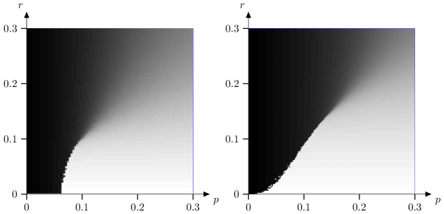
Figure 1: Density $\overline{\rho}$ of the upper invariant law of two monotone cellular automata as a function of the parameters, shown on a scale from 0 (white) to 1 (black). On the left: a version of Toom’s model that applies the maps $\mathchar 0\relax^{0}$, $\mathchar 0\relax^{1}$, and $\mathchar 0\relax^{\rm NEC}$ with probabilities $p$, $r$, and $1-p-r$, respectively. On the right: the mononotone random cellular automaton that applies the maps $\mathchar 0\relax^{0}$, $\mathchar 0\relax^{1}$, and $\mathchar 0\relax^{\rm NN}$ with probabilities $p$, $r$, and $1-p-r$, respectively. Contrary to $\mathchar 0\relax^{\rm NEC}$, the map $\mathchar 0\relax^{\rm NN}$ is not an eroder. By the symmetry between the 0’s and the 1’s, in both models, the density $\underline{\rho}$ of the lower invariant law equals $1-\overline{\rho}$. Due to metastability effects, the area where the upper invariant law differs from the lower invariant law is shown too large in these numerical data. For Toom’s model with $r=0$, the data shown above suggest a first order phase transition at $p_{\rm c}\approx 0.057$ but based on numerical data for edge speeds we believe the true value is $p_{\rm c}\approx 0.053$. We conjecture that the model on the right has a unique invariant law everywhere except on the diagonal $p=r$ for $p$ sufficiently small.

1.3 Main results

While Toom’s stability theorem is an impressive result, it is important to realise its limitations. As Toom already remarked [Too80, Section V], his theorem does not apply to monotone cellular automata whose local state space is not $\{0,1\}$, but $\{0,1,2\}$, for example. Also, his theorem only applies in discrete time and only to random perturbations of cellular automata defined by a single non-constant monotonic map $\mathchar 0\relax$.

The most difficult part in the proof of Toom’s stability theorem is showing that if $\mathchar 0\relax$ is an eroder, then $\overline{\rho}(p)\to 1$ as $p\to 0$. To give a lower bound on $\overline{\rho}(p)$ for small values of $p$, Toom uses a Peierls contour argument. The main result of our article is extending this Peierls argument to monotone cellular automata whose definition involves, apart from the constant monotonic map $\mathchar 0\relax^{0}$, several non-constant monotonic maps $\mathchar 0\relax_{1},\ldots,\mathchar 0\relax_{m}$. We are especially interested in the case when one of these maps is the identity map $\mathchar 0\relax^{\rm id}$ and in the closely related problem of giving lower bounds on $\overline{\rho}(p)$ for monotone interacting particle systems, which evolve in continuous time. Another result of our work is obtaining explicit lower bounds for $\overline{\rho}(p)$ for concrete models, which has not been attempted very much.

In particular, we extend Toom’s definition of a contour to monotone cellular automata that apply several non-constant monotonic maps and to monotone interacting particle systems. We show that $X_{n}(i)=0$ for some $i\in{\mathbb{Z}}^{d}$ (or equivalently $X_{t}(i)=0$ in continuous time) implies the presence of a Toom contour “rooted at” $(n,i)$ (or $(t,i)$ respectively), which in turn can be used to obtain lower bounds for $\overline{\rho}(p)$ via a Peierls argument. Our main results are contained in Theorems 7, 9 and 41. At this point rather than formally stating these results, which would require dwelling into technical details, we state the explicit bounds we obtain as a result of our construction.

Our extension of Toom’s result allows us to establish or improve explicit lower bounds for $\overline{\rho}(p)$ for concrete models. First we consider Toom’s set-up, that is monotone random cellular automata that apply the maps $\mathchar 0\relax^{0}$ and $\mathchar 0\relax$ with probabilities $p$ and $1-p$, respectively, where $\mathchar 0\relax$ is an eroder. An easy coupling argument shows that the intensity $\overline{\rho}(p)$ of the upper invariant law is a nonincreasing function of $p$, so we can define a critical parameter

$$p_{\rm c}:=\sup\{p:\overline{\rho}(p)>0\}\in[0,1].$$ (1.10)

Since $\mathchar 0\relax$ is an eroder, Toom’s stability theorem tells us that $p_{\rm c}>0$. We show how to derive explicit lower bounds on $p_{\rm c}$ for any choice of the eroder $\mathchar 0\relax$, and do this for two concrete examples. We first take for $\mathchar 0\relax$ the map $\mathchar 0\relax^{\rm NEC}$ and obtain the bound $p_{\rm c}\geq 3^{-21}$, which does not compare well to the estimated value $p_{\rm c}\approx 0.053$ coming from numerical simulations. Nevertheless, this is probably the best rigorous bound currently available. Then we take for $\mathchar 0\relax$ the map $\mathchar 0\relax^{\rm coop}$ and, improving on Toom’s method, we get the bound $p_{\rm c}\geq 1/64$. This is also some way off the estimated value $p_{\rm c}\approx 0.105$ coming from numerical simulations.

Then we consider the monotone random cellular automaton on ${\mathbb{Z}}^{d}$ that applies the maps $\mathchar 0\relax^{0},\mathchar 0\relax^{\rm id}$, and $\mathchar 0\relax^{\rm coop}$ with probabilities $p,q,r$, respectively with $q=1-p-r$. For each $p,r\geq 0$ such that $p+r\leq 1$, let $\overline{\rho}(p,r)$ denote the intensity of the upper invariant law of the process with parameters $p,1-p-r,r$. Arguing as before, it is easy to see that for each $0\leq r<1$ we can define a critical parameter

$$p_{\rm c}(r):=\sup\{p:\overline{\rho}(p,r)>0\}\in[0,1-r].$$ (1.11)

By carefully examining the structure of Toom contours for this model, we prove the bound $p_{c}(r)>0.00624r$.

Finally, we consider the interacting particle system on ${\mathbb{Z}}^{2}$ that applies the monotonic maps $\mathchar 0\relax^{0}$ and $\mathchar 0\relax^{\rm coop}$ with rates $1$ and $\lambda$, respectively. This model was introduced by Durrett [Dur86] as the sexual contact process, and we can think of it as the limit of the previous discrete-time cellular automata. For each $\lambda>0$ we let $\overline{\rho}(\lambda)$ denote the intensity of the upper invariant law of the process with parameters $1,\lambda$. Again, we define a critical parameter

$$\lambda_{\rm c}:=\inf\{\lambda\geq 0:\overline{\rho}(\lambda)>0\}\in(0,\infty).$$ (1.12)

Numerical simulations suggest the value $\lambda_{\rm c}\approx 12.4$, we show the upper bound $\lambda_{\rm c}\leq 161.1985$. Durrett claimed a proof that $\lambda_{\rm c}\leq 110$, which he describes as ridiculous, but for which he challenges the reader to do better. We have quite not managed to beat his bound, though we are not far off. The proofs of all results in [Dur86] are claimed to be contained in a forthcoming paper with Lawrence Gray [DG85] that has never appeared. In [Gra99], Gray refered to these proofs as “unpublished” and in [BD17], Durrett cites the paper as an “unpublished manuscript”.

Although for monotone cellular automata that apply several non-constant monotonic maps and for monotone interacting particle systems our methods do not seem to be enough to obtain bounds on the critical value in general, we believe that our examples are instructive of how one can try to do it for a concrete model.

1.4 Discussion

The cellular automaton defined by the NEC voting map $\mathchar 0\relax^{\rm NEC}$ is nowadays known as Toom’s model. In line with Stigler’s law of eponymy, Toom’s model was not invented by Toom, but by Vasilyev, Petrovskaya, and Pyatetski-Shapiro, who simulated random perturbations of this and other models on a computer [VPP69]. The function $p\mapsto\overline{\rho}(p)$ appears to be continuous except for a jump at $p_{\rm c}$ (see Figure 1). Toom, having heard of [VPP69] during a seminar, proved in [Too74] that there exist random cellular automata on ${\mathbb{Z}}^{d}$ with at least $d$ different invariant laws. Although Toom’s model is not explicitly mentioned in the paper, his proof method can be applied to prove that $p_{\rm c}>0$ for his model.

In [Too80], Toom improved his methods and proved his celebrated stability theorem. His paper is quite hard to read. One of the reasons is that Toom tries to be as general as possible. For example, he allows for cellular automata that look back more than one step in time, which severely complicates the statement of conditions like (1.9). He also allows for noise that is not i.i.d. and cellular automata that are not monotone, even though all his results in the general case can easily be obtained by comparison with the i.i.d. monotone case. Toom’s Peierls argument in the original paper is quite hard to understand. A more accessible account of Toom’s original argument (with pictures!) in the special case of Toom’s model can be found in the appendix of [LMS90]. Although in principle, Toom’s Peierls argument can be used to derive explicit bounds on $p_{\rm c}$, Toom did not attempt to do so, no doubt in the belief that more powerful methods would be developed in due time.

Bramson and Gray [BG91] have given another alternative proof of Toom’s stability theorem that relies on comparison with continuum models (which describe unions of convex sets in ${\mathbb{R}}^{d}$ evolving in continuous time) and renormalisation-style block arguments. They somewhat manage to relax Toom’s conditions but the proof is very heavy and any explicit bounds derived using this method would presumably be very bad. Gray [Gra99] proved a stability theorem for monotone interacting particle systems. The proofs use ideas from [Too80] and [BG91] and do not lend themselves well to the derivation of explicit bounds. Gray also derived necessary and sufficient conditions for a monotonic map to be an eroder [Gra99, Thm 18.2.1], apparently overlooking the fact that Toom had already proved the much simpler condition (1.9).

Motivated by abstract problems in computer science, a number of authors have given alternative proofs of Toom’s stability theorem in a more restrictive setting [GR88, BS88, Gac95, Gac21]. Their main interest is in a three-dimensional system which evolves in two steps: letting $e_{1},e_{2},e_{3}$ denote the basis vectors in ${\mathbb{Z}}^{3}$, they first replace $X_{n}(i)$ by

$$X^{\prime}_{n}(i):={\tt round}\big{(}(X_{n}(i)+X_{n}(i+e_{1})+X_{n}(i+e_{2}))/3\big{)},$$

and then set

$$X_{n+1}(i):={\tt round}\big{(}(X^{\prime}_{n}(i)+X^{\prime}_{n}(i+e_{3})+X^{\prime}_{n}(i-e_{3}))/3\big{)}.$$

They prove explicit bounds for finite systems, although for values of $p$ that are extremely close to zero. The proofs of [GR88] do not use Toom’s Peierls argument but rely on different methods. Their bounds were improved in [BS88]. Still better bounds can be found in the unpublished note [Gac95]. The proofs in the latter manuscript are very similar to Toom’s argument, with some crucial improvements at the end that are hard to follow due to missing definitions. This version of the argument seems to have inspired the incomplete note by John Preskill [Pre07] who links it to the interesting idea of counting “minimal explanations”. His definition of a “minimal explanation” is a bit stronger than the definition we will adopt in Subsection 7.1 below, but sometimes, such as in the picture in Figure 3 on the right, the two definitions coincide. Figure 3 shows that the relation between Toom contours and minimal explanations is not so straightforward as suggested in [Gac95, Pre07]. We have not found a good way to control the number of minimal explanations with a given number of defective sites and we do not know how to derive the lower bounds on the density of the upper invariant law stated in [Gac95, Pre07].

Hwa-Nien Chen [Che92, Che94], who was a PhD student of Lawrence Gray, studied the stability of various variations of Toom’s model under perturbations of the initial state and the birth rate. The proofs of two of his four theorems depend on results that he cites from the as yet nonexisting paper [DG85]. Ponselet [Pon13] gave an excellent account of the existing literature and together with her supervisor proved exponential decay of correlations for the upper invariant law of a large class of randomly perturbed monotone cellular automata [MP11].

There exists duality theory for general monotone interacting particle systems [Gra86, SS18]. The basic idea is that the state in the origin at time zero is a monotone function of the state at time $-t$, and this monotone function evolves in a Markovian way as a function of $t$. Durrett [Dur86] mentions this dual process as an important ingredient of the proofs of the forthcoming paper [DG85] and it is also closely related to the minimal explanations of Preskill [Pre07]. A good understanding of this dual process could potentially help solve many open problems in the area, but its behaviour is already quite complicated in the mean-field case [MSS20].

1.5 Outline

The paper is organized as follows. We define Toom contours and give an outline of the main idea of the Peierls argument in Subsection 2.1. In Subsection 2.2 we prove Toom’s stability theorem. In Susbsection 2.3 we introduce a stronger notion of Toom contours, that allows us to improve bounds for certain models. We then present two explicit bounds in Toom’s set-up in Subsection 2.4. In Subsection 2.5 we consider monotone random cellular automata that apply several non-constant monotonic maps and in Subsection 2.6 we discuss continuous time results and bounds.

The rest of the paper is devoted for proofs and technical arguments. The results stated in Subsections 2.1 are proved in Section 3. Section 4 contains all the proofs of the results stated in Subsections 2.2, 2.3 and 2.4. The results of Subsection 2.5 are proved in Section 5. Section 6 gives the precise definitions and results together with their proofs in the continuous-time setting. Finally, the relation between Toom contours and minimal explanations in the sense of John Preskill [Pre07] is discussed in Section 7, where we also discuss the open problem of counting minimal explanations.

2 Setting and definitions

2.1 Toom’s Peierls argument

In this subsection, we derive a lower bound on the intensity of the upper invariant law for a class of monotone random cellular automata. We use a Peierls argument based on a special type of contours that we will call Toom contours. In their essence, these are the contours used in [Too80], though on the face of it our definitions will look a bit different from those of [Too80]. This pertains especially to the “sources” and “sinks” defined below that are absent from Toom’s formulation and that we think help elucidate the argument. We start by defining a special sort of directed graphs, which we will call Toom graphs (see Figure 2). After that we first give an outline of the main idea of the Peierls argument and then provide the details.

Toom graphs

Recall that a directed graph is a pair $(V,\vec{E})$ where $V$ is a set whose elements are called vertices and $\vec{E}$ is a subset of $V\times V$ whose elements are called directed edges. For each directed edge $(v,w)\in E$, we call $v$ the starting vertex and $w$ the endvertex of $(v,w)$. We let

$$\vec{E}_{\rm in}(v):=\big{\{}(u,v^{\prime})\in\vec{E}:v^{\prime}=v\big{\}}\quad\mbox{and}\quad\vec{E}_{\rm out}(v):=\big{\{}(v^{\prime},w)\in\vec{E}:v^{\prime}=v\big{\}}$$ (2.1)

denote the sets or directed edges entering and leaving a given vertex $v\in V$, respectively.

We will need to generalise the concept of a directed graph by allowing directed edges to have a type in some finite set $\{1,\ldots,\sigma\}$, with the possibility that several edges of different types connect the same two vertices. To that aim, we define an directed graph with $\sigma$ types of edges to be a pair $(V,{\cal E})$, where ${\cal E}=(\vec{E}_{1},\ldots,\vec{E}_{\sigma})$ is a sequence of subsets of $V\times V$. We interpret $\vec{E}_{s}$ as the set of directed edges of type $s$.

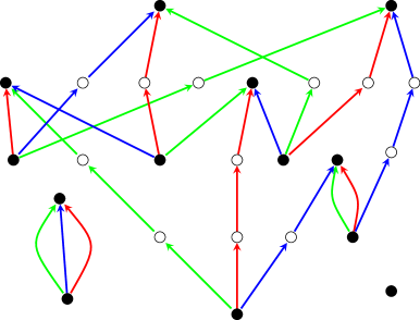
Figure 2: Example of a Toom graph with three charges. Sources and sinks are indicated with solid dots and internal vertices are indicated with open dots. Note the isolated vertex in the lower right corner, which is a source and a sink at the same time.

Definition 1

A Toom graph with $\sigma\geq 2$ charges is a directed graph with $\sigma$ types of edges $(V,{\cal E})=(V,\vec{E}_{1},\ldots,\vec{E}_{\sigma})$ such that each vertex $v\in V$ satisfies one of the following four conditions:

1. $|\vec{E}_{s,{\rm in}}(v)|=0=|\vec{E}_{s,{\rm out}}(v)|$ for all $1\leq s\leq\sigma$,

2. $|\vec{E}_{s,{\rm in}}(v)|=0$ and $|\vec{E}_{s,{\rm out}}(v)|=1$ for all $1\leq s\leq\sigma$,

3. $|\vec{E}_{s,{\rm in}}(v)|=1$ and $|\vec{E}_{s,{\rm out}}(v)|=0$ for all $1\leq s\leq\sigma$,

4. there exists an $s\in\{1,\ldots,\sigma\}$ such that $|\vec{E}_{s,{\rm in}}(v)|=1=|\vec{E}_{s,{\rm out}}(v)|$
   and $|\vec{E}_{l,{\rm in}}(v)|=0=|\vec{E}_{l,{\rm out}}(v)|$ for each $l\neq s$.

See Figure 2 for a picture of a Toom graph with three charges. We set

$$\begin{array}[]{r@{\,}c@{\,}l}\displaystyle V_{\circ}&:=&\displaystyle\big{\{}v\in V:|\vec{E}_{s,{\rm in}}(v)|=0\ \;\forall 1\leq s\leq\sigma\big{\}},\\[5.0pt] \displaystyle V_{\ast}&:=&\displaystyle\big{\{}v\in V:|\vec{E}_{s,{\rm out}}(v)|=0\ \;\forall 1\leq s\leq\sigma\big{\}},\\[5.0pt] \displaystyle V_{s}&:=&\displaystyle\big{\{}v\in V:|\vec{E}_{s,{\rm in}}(v)|=1=|\vec{E}_{s,{\rm out}}(v)|\big{\}}\qquad(1\leq s\leq\sigma).\end{array}$$ (2.2)

Vertices in $V_{\circ},V_{\ast}$, and $V_{s}$ are called sources, sinks, and internal vertices with charge $s$, respectively. Vertices in $V_{\circ}\cap V_{\ast}$ are called isolated vertices. Informally, we can imagine that at each source there emerge $\sigma$ charges, one of each type, that then travel via internal vertices of the corresponding charge through the graph until they arrive at a sink, in such a way that at each sink there converge precisely $\sigma$ charges, one of each type. It is clear from this description that $|V_{\circ}|=|V_{\ast}|$, i.e., the number of sources equals the number of sinks.

We let $\vec{E}:=\bigcup_{s=1}^{\sigma}\vec{E}_{s}$ denote the union of all directed edge sets and we let $E:=\big{\{}\{v,w\}:(v,w)\in\vec{E}\big{\}}$ denote the corresponding set of undirected edges. We say that a Toom graph $(V,{\cal E})$ is connected if the associated undirected graph $(V,E)$ is connected.

Toom contours

Our next aim is to define Toom contours, which are connected Toom graphs that are embedded in space-time ${\mathbb{Z}}^{d+1}$ in a special way. Let $(V,{\cal E})=(V,\vec{E}_{1},\ldots,\vec{E}_{\sigma})$ be a Toom graph with $\sigma$ charges. Recall that $\vec{E}=\bigcup_{s=1}^{\sigma}\vec{E}_{s}$.

Definition 2

An embedding of $(V,{\cal E})$ is a map

$$V\ni v\mapsto\psi(v)=\big{(}\vec{\psi}(v),\psi_{d+1}(v)\big{)}\in{\mathbb{Z}}^{d}\times{\mathbb{Z}}$$ (2.3)

that has the following properties:

1. $\displaystyle\psi_{d+1}(w)=\psi_{d+1}(v)-1$ for all $(v,w)\in\vec{E}$,

2. $\psi(v_{1})\neq\psi(v_{2})$ for each $v_{1}\in V_{\ast}$ and $v_{2}\in V$ with $v_{1}\neq v_{2}$,

3. $\psi(v_{1})\neq\psi(v_{2})$ for each $v_{1},v_{2}\in V_{s}$ with $v_{1}\neq v_{2}$ $(1\leq s\leq\sigma)$.

We interpret $\vec{\psi}(v)$ and $\psi_{d+1}(v)$ as the space and time coordinates of $\psi(v)$ respectively. Condition (i) says that directed edges $(v,w)$ of the Toom graph $(V,\vec{E})$ point in the direction of decreasing time. Condition (ii) says that sinks do not overlap with other vertices and condition (iii) says that internal vertices do not overlap with other internal vertices of the same charge. See Figure 3 for an example of an embedding of a Toom graph. Not every Toom graph can be embedded. Indeed, it is easy to see that if $(V,{\cal E})$ has an embedding in the sense defined above, then

$$|\vec{E}_{1}|=\cdots=|\vec{E}_{\sigma}|,$$ (2.4)

i.e., there is an equal number of charged edges of each charge. The Toom graph of Figure 2 can be embedded, but if we would change the number of internal vertices on one of the paths from a source to a sink, then the resulting graph would still be a Toom graph but it would not be possible to embed it.

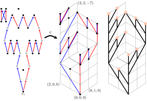
Figure 3: On the left: a Toom graph with two charges. Middle: embedding of the Toom graph on the left, with time running downwards. The connected component containing the root $v_{\circ}$ forms a Toom contour rooted at the origin $(0,0,0)$. On the right: a minimal explanation for a monotone cellular automaton $\Phi$ that applies the maps $\mathchar 0\relax^{0}$ and $\mathchar 0\relax^{\rm coop}$ with probabilities $p$ and $1-p$, respectively. The origin has the value zero because the sites marked with a star are defective. This explanation is minimal in the sense that removing any of the defective sites results in the origin having the value one. The Toom contour in the middle picture is present in $\Phi$. In particular, the sinks of the Toom contour coincide with some, though not with all of the defective sites of the minimal explanation.

Definition 3

A Toom contour is a quadruple $(V,{\cal E},v_{\circ},\psi)$, where $(V,{\cal E})$ is a connected Toom graph, $v_{\circ}\in V_{\circ}$ is a specially designated source, and $\psi$ is an embedding of $(V,{\cal E})$ that has the additional properties that:

1. $\psi_{d+1}(v_{\circ})>t$ for all $(i,t)\in\psi(V)\backslash\{\psi(v_{\circ})\}$,

where $\psi(V):=\{\psi(v):v\in V\}$ denotes the image of $V$ under $\psi$.

We call $v_{\circ}$ the root of the Toom contour and we say that the Toom contour $(V,{\cal E},v_{\circ},\psi)$ is rooted at the space-time point $\psi(v_{\circ})\in{\mathbb{Z}}^{d+1}$. See Figure 3 for an example of a Toom contour with two charges.

For any Toom contour $(V,{\cal E},v_{\circ},\psi)$, we write

$$\begin{array}[]{l}\vec{E}^{\ast}:=\bigcup_{s=1}^{\sigma}\vec{E}^{\ast}_{s}\quad\mbox{with}\quad\vec{E}^{\ast}_{s}:=\big{\{}(v,w)\in\vec{E}_{s}:v\in V_{s}\cup\{v_{\circ}\}\big{\}}\quad(1\leq s\leq\sigma),\\[5.0pt] \vec{E}^{\circ}:=\bigcup_{s=1}^{\sigma}\vec{E}^{\circ}_{s}\quad\mbox{with}\quad\vec{E}^{\circ}_{s}:=\big{\{}(v,w)\in\vec{E}_{s}:v\in V_{\circ}\backslash\{v_{\circ}\}\big{\}}\quad(1\leq s\leq\sigma).\end{array}$$ (2.5)

i.e., $\vec{E}^{\ast}$ is the set of directed edges that have an internal vertex or the root as their starting vertex, and $\vec{E}^{\circ}$ are all the other directed edges, that start at a source that is not the root. The special role played by the root will become important in the next subsection, when we define what it means for a Toom contour to be present in a collection of i.i.d. monotonic maps.

If $(V,{\cal E},v_{\circ},\psi)$ is a Toom contour, then we let

$$\begin{array}[]{c}\displaystyle\psi(V_{\ast}):=\big{\{}\psi(v):v\in V_{\ast}\big{\}},\quad\psi(\vec{E}^{\ast}_{s}):=\big{\{}\big{(}\psi(v),\psi(w)\big{)}:(v,w)\in\vec{E}^{\ast}_{s}\big{\}},\\[5.0pt] \psi(\vec{E}^{\circ}_{s}):=\big{\{}\big{(}\psi(v),\psi(w)\big{)}:(v,w)\in\vec{E}^{\circ}_{s}\big{\}}\qquad(1\leq s\leq\sigma),\end{array}$$ (2.6)

denote the images under $\psi$ of the set of sinks $V_{\ast}$ and the sets of directed edges $\vec{E}^{\ast}_{s}$ and $\vec{E}^{\circ}_{s}$, respectively. We call two Toom contours $(V,{\cal E},v_{\circ},\psi)$ and $(V^{\prime},{\cal E}^{\prime},v^{\prime}_{\circ},\psi^{\prime})$ equivalent if

$$\psi(v_{\circ})=\psi^{\prime}(v_{\circ}),\quad\psi(V_{\ast})=\psi^{\prime}(V^{\prime}_{\ast}),\quad\psi(\vec{E}^{\ast}_{s})=\psi^{\prime}(\vec{E^{\prime}}^{\ast}_{s}),\quad\psi(\vec{E}^{\circ}_{s})=\psi^{\prime}(\vec{E^{\prime}}^{\circ}_{s}).$$ (2.7)

The main idea of the construction

We will be interested in monotone random cellular automata that are defined by a probability distribution $p_{0},\ldots,p_{m}$ and monotonic maps $\mathchar 0\relax_{0},\ldots,\mathchar 0\relax_{m}$, of which $\mathchar 0\relax_{0}=\mathchar 0\relax^{0}$ is the constant map that always gives the outcome zero and $\mathchar 0\relax_{1},\ldots,\mathchar 0\relax_{m}$ are non-constant. This generalises Toom’s set-up, who only considered the case $m=1$. We fix an i.i.d. collection $\Phi=(\Phi_{(i,t)})_{(i,t)\in{\mathbb{Z}}^{d+1}}$ of monotonic maps such that ${\mathbb{P}}[\Phi_{(i,t)}=\mathchar 0\relax_{k}]=p_{k}$ $(0\leq k\leq m)$. A space-time point $(i,t)$ with $\Phi_{(i,t)}=\mathchar 0\relax^{0}$ is called a defective site. In Lemmas 4 and 5 below, we show that $\Phi$ almost surely determines a stationary process $(\overline{X}_{t})_{t\in{\mathbb{Z}}}$ that at each time $t$ is distributed according to the upper invariant law $\overline{\nu}$. Our aim is to give an upper bound on the probability that $\overline{X}_{0}(0)=0$, which then translates into a lower bound on the intensity $\overline{\rho}$ of the upper invariant law.

To achieve this, we first describe a special way to draw a Toom graph inside space-time ${\mathbb{Z}}^{d+1}$. Such an embedding of a Toom graph in space-time is then called a Toom contour. Since our argument requires looking backwards in time, it will be convenient to adopt the convention that in all our pictures (such as Figure 3), time runs downwards. Next, we define when a Toom contour is present in the random collection of maps $\Phi$. Theorem 7 then states that the event $\overline{X}_{0}(0)=0$ implies the presence of a Toom contour in $\Phi$. This allows us to bound the probability that $\overline{X}_{0}(0)=0$ from above by the expected number of Toom contours that are present in $\Phi$. In later subsections, we will then discuss conditions under which this expectation can be controlled and derive explicit bounds.

Before we state the remaining definitions, which are mildly complicated, we explain the main idea of the construction. We will define presence of Toom contours in such a way that the space-time point $(0,0)$ is a source and all the sinks correspond to defective sites where the map $\mathchar 0\relax^{0}$ is applied. Let $M_{n}$ denote the number of Toom contours that have $(0,0)$ as a source and that have $n$ sinks. One would like to show that if the map $\mathchar 0\relax^{0}$ is applied with a sufficiently small probability $p$, then the expression $\sum_{n=1}^{\infty}M_{n}p^{n}$ is small. This will not be true, however, unless one imposes additional conditions on the contours. In fact, it is rather difficult to control the number of contours with a given number of sinks. It is much easier to count contours with a given number of edges. Letting $N_{n}$ denote the number of contours with $n$ edges (rather than sinks), it is not hard to show that $N_{n}$ grows at most exponentially as a function of $n$.

To complete the argument, therefore, it suffices to impose additional conditions on the contours that bound the number of edges in terms of the number of sinks. If at a certain space-time point $(i,t)$, the stationary process satisfies $\overline{X}_{t}(i)=0$, and the map $\Phi_{(i,t)}$ that is applied there is $\mathchar 0\relax_{k}$, then for each set $A\in{\cal A}(\mathchar 0\relax_{k})$ (with ${\cal A}(\mathchar 0\relax_{k})$ defined in (1.8)), at least one of the sites $j\in A$ must have the property that $\overline{X}_{t-1}(j)=0$. We will use this to steer edges in a certain direction, in such a way that different charges tend to move away from each other, except for edges that originate in a source.

Since in the end, edges of all charges must convene in each sink, this will allow us to bound the total number of edges in terms of the “bad” edges that originate in a source. Equivalently, this allows us to bound the total number of edges in terms of the number of sources, which is the same as the number of sinks. This is the main idea of the argument. We now continue to give the precise definitions.

The contour argument

Having defined the right sort of contours, we now come to the core of the argument: the fact that $\overline{X}_{0}(0)=0$ implies the existence of a Toom contour with certain properties. We first need a special construction of the stationary process $(\overline{X}_{t})_{t\in{\mathbb{Z}}}$. We let $\{0,1\}^{{\mathbb{Z}}^{d+1}}$ denote the space of all space-time configurations $x=(x_{t}(i))_{(i,t)\in{\mathbb{Z}}^{d+1}}$. For $x\in\{0,1\}^{{\mathbb{Z}}^{d+1}}$ and $t\in{\mathbb{Z}}$, we define $x_{t}\in\{0,1\}^{{\mathbb{Z}}^{d}}$ by $x_{t}:=(x_{t}(i))_{i\in{\mathbb{Z}}^{d}}$. We will call a collection ${\bm{\mathchar 0\relax}}=(\mathchar 0\relax_{(i,t)})_{(i,t)\in{\mathbb{Z}}^{d+1}}$ of monotonic maps from $\{0,1\}^{{\mathbb{Z}}^{d}}$ to $\{0,1\}$ a monotonic flow. By definition, a trajectory of ${\bm{\mathchar 0\relax}}$ is a space-time configuration $x$ such that

$$x_{t}(i)=\mathchar 0\relax_{(i,t)}(\theta_{i}x_{t-1})\qquad\big{(}(i,t)\in{\mathbb{Z}}^{d+1}\big{)}.$$ (2.8)

We need the following two simple lemmas.

Lemma 4 (Minimal and maximal trajectories)

Let ${\bm{\mathchar 0\relax}}$ be a monotonic flow. Then there exist trajectories $\underline{x}$ and $\overline{x}$ that are uniquely characterised by the property that each trajectory $x$ of ${\bm{\mathchar 0\relax}}$ satisfies $\underline{x}\leq x\leq\overline{x}$ (pointwise).

Lemma 5 (The lower and upper invariant laws)

Let $\mathchar 0\relax_{0},\ldots,\mathchar 0\relax_{m}$ be monotonic functions, let $p_{0},\ldots,p_{m}$ be a probability distribution, and let $\underline{\nu}$ and $\overline{\nu}$ denote the lower and upper invariant laws of the corresponding monotone random cellular automaton. Let $\Phi=\big{(}\Phi_{(i,t)}\big{)}_{(i,t)\in{\mathbb{Z}}^{d+1}}$ be an i.i.d. collection of monotonic maps such that ${\mathbb{P}}[\Phi_{(i,t)}=\mathchar 0\relax_{k}]=p_{k}$ $(0\leq k\leq m)$, and let $\underline{X}$ and $\overline{X}$ be the minimal and maximal trajectories of $\Phi$. Then for each $t\in{\mathbb{Z}}$, the random variables $\underline{X}_{t}$ and $\overline{X}_{t}$ are distributed according to the laws $\underline{\nu}$ and $\overline{\nu}$, respectively.

From now on, we fix a monotonic flow ${\bm{\mathchar 0\relax}}$ that takes values in $\{\mathchar 0\relax_{0},\ldots,\mathchar 0\relax_{m}\}$, of which $\mathchar 0\relax_{0}=\mathchar 0\relax^{0}$ is the constant map that always gives the outcome zero and $\mathchar 0\relax_{1},\ldots,\mathchar 0\relax_{m}$ are non-constant. Recall that ${\cal A}(\mathchar 0\relax_{k})$, defined in (1.8), corresponds to the set of minimal configurations on which $\mathchar 0\relax_{k}$ gives the outcome 1. We fix an integer $\sigma\geq 2$ and for each $1\leq k\leq m$ and $1\leq s\leq\sigma$, we choose a set

$$A_{s}(\mathchar 0\relax_{k})\in{\cal A}(\mathchar 0\relax_{k}).$$ (2.9)

Informally, the aim of these sets is to steer edges of different charges away from each other. In later subsections, when we derive bounds for concrete models, we will make an explicit choice for $\sigma$ and sets $A_{s}(\mathchar 0\relax_{k})$. For the moment, we allow these to be arbitrary. The integer $\sigma$ corresponds to the number of charges. The definition of what it means for a contour to be present will depend on the choice of the sets in (2.9).

As a concrete example, consider the case $m=1$ and $\mathchar 0\relax_{1}=\mathchar 0\relax^{\rm coop}$, the cooperative branching map defined in (1.7). The set ${\cal A}(\mathchar 0\relax^{\rm coop})$ from (1.8) is given by ${\cal A}(\mathchar 0\relax^{\rm coop})=\{A_{1},A_{2}\}$ with $A_{1}:=\{(0,0)\}$ and $A_{2}:=\{(0,1),(1,0)\}$. Using (1.9) we see that $\mathchar 0\relax^{\rm coop}$ is an eroder. In this concrete example, we will set $\sigma:=2$ and for the sets $A_{s}(\mathchar 0\relax_{1})$ $(s=1,2)$ of (2.9) we choose the sets $A_{1},A_{2}$ we have just defined.

Definition 6

A Toom contour $(V,{\cal E},v_{\circ},\psi)$ with $\sigma$ charges is present in the monotonic flow ${\bm{\mathchar 0\relax}}$ if:

1. $\displaystyle\mathchar 0\relax_{\psi(v)}=\mathchar 0\relax^{0}$ for all $\displaystyle v\in V_{\ast}$,

2. $\displaystyle\mathchar 0\relax_{\psi(v)}\in\{\mathchar 0\relax_{1},\ldots,\mathchar 0\relax_{m}\}$ for all $\displaystyle v\in V\backslash V_{\ast}$,

3. $\displaystyle\vec{\psi}(w)-\vec{\psi}(v)\in A_{s}(\mathchar 0\relax_{\psi(v)})$ for all $(v,w)\in\vec{E}^{\ast}_{s}$ $(1\leq s\leq\sigma$),

4. $\displaystyle\vec{\psi}(w)-\vec{\psi}(v)\in\bigcup_{s=1}^{\sigma}A_{s}(\mathchar 0\relax_{\psi(v)})$ for all $(v,w)\in\vec{E}^{\circ}$,

where $\vec{E}^{\ast}_{s}$ and $\vec{E}^{\circ}$ are defined in (2.5) and $\vec{\psi}(v)$, defined in (2.3), denotes the spatial coordinates of the space-time point $\psi(v)$.

Note that the definition of what it means for a contour to be present depends on the choice of the sets $A_{s}(\mathchar 0\relax_{k})$ in (2.9). Conditions (i) and (ii) say that sinks of $(V,{\cal E})$ are mapped to defective space-time points, where the constant map $\mathchar 0\relax^{0}$ is applied, and all other vertices are mapped to space-time points where one of the non-constant maps $\mathchar 0\relax_{1},\ldots,\mathchar 0\relax_{m}$ is applied. Together with our earlier definition of an embedding, condition (iii) says that if $(v,w)$ is an edge with charge $s$ that comes out of the root or an internal vertex, then $(v,w)$ is mapped to a pair of space-time points of the form $\big{(}(i,t),(i+j,t-1)\big{)}$ with $j\in A_{s}(\mathchar 0\relax_{\psi(v)})$. Condition (iv) is similar, except that if $v$ is a source different from the root, then we only require that $j\in\bigcup_{s=1}^{\sigma}A_{s}(\mathchar 0\relax_{\psi(v)})$. It is clear from this definition that if $(V,{\cal E},v_{\circ},\psi)$ and $(V^{\prime},{\cal E}^{\prime},v^{\prime}_{\circ},\psi^{\prime})$ are equivalent Toom contours, then $(V,{\cal E},v_{\circ},\psi)$ is present in ${\bm{\mathchar 0\relax}}$ if and only if the same is true for $(V^{\prime},{\cal E}^{\prime},v^{\prime}_{\circ},\psi^{\prime})$.

For our example of the monotone cellular automaton with $\mathchar 0\relax_{1}=\mathchar 0\relax^{\rm coop}$, Definition 6 is demonstrated in Figure 3. Directed edges of charge 1 and 2 are indicated in red and blue, respectively. Because of our choice $A_{2}(\mathchar 0\relax_{1}):=\{(0,1),(1,0)\}$, blue edges that start at internal vertices or the root point in directions where one of the spatial coordinates increases by one. Likewise, since $A_{1}(\mathchar 0\relax_{1}):=\{(0,0)\}$, red edges that start at internal vertices or the root point straight up, i.e., in the direction of decreasing time. Sinks of the Toom contour correspond to defective sites, as indicated in Figure 3 on the right.

In view of Lemma 5, the following crucial theorem links the upper invariant law to Toom contours.

Theorem 7 (Presence of a Toom contour)

Let ${\bm{\mathchar 0\relax}}$ be a monotonic flow on $\{0,1\}^{{\mathbb{Z}}^{d}}$ that take values in $\{\mathchar 0\relax_{0},\ldots,\mathchar 0\relax_{m}\}$, where $\mathchar 0\relax_{0}=\mathchar 0\relax^{0}$ is the constant map that always gives the outcome zero and $\mathchar 0\relax_{1},\ldots,\mathchar 0\relax_{m}$ are non-constant. Let $\overline{x}$ denote the maximal trajectory of ${\bm{\mathchar 0\relax}}$. Let $\sigma\geq 2$ be an integer and for each $1\leq s\leq\sigma$ and $1\leq k\leq m$, let $A_{s}(\mathchar 0\relax_{k})\in{\cal A}(\mathchar 0\relax_{k})$ be fixed. If $\overline{x}_{0}(0)=0$, then, with respect to the given choice of $\sigma$ and the sets $A_{s}(\mathchar 0\relax_{k})$, a Toom contour $(V,{\cal E},v_{\circ},\psi)$ rooted at $(0,0)$ is present in ${\bm{\mathchar 0\relax}}$.

We note that the converse of Theorem 7 does not hold, i.e., the presence in ${\bm{\mathchar 0\relax}}$ of a Toom contour $(V,{\cal E},v_{\circ},\psi)$ that is rooted at $(0,0)$ does not imply that $\overline{X}_{0}(0)=0$. This can be seen from Figure 3. In this example, if there would be no other defective sites apart from the sinks of the Toom contour, then the origin would have the value one. This is a difference with the Peierls arguments used in percolation theory, where the presence of a contour is a necessary and sufficient condition for the absence of percolation.

Let ${\cal T}_{0}$ denote the set of Toom contours rooted at $(0,0)$ (up to equivalence). We formally denote a Toom contour by $T=(V,E,v_{\circ},\psi)$. Let $\Phi=(\Phi_{(i,t)})_{(i,t)\in{\mathbb{Z}}^{d+1}}$ be an i.i.d. collection of monotonic maps taking values in $\{\mathchar 0\relax_{0},\ldots,\mathchar 0\relax_{m}\}$. Then Theorem 7 implies the Peierls bound:

$$1-\overline{\rho}={\mathbb{P}}[\overline{X}_{0}(0)=0]\leq\sum_{T\in{\cal T}_{0}}{\mathbb{P}}\big{[}T\mbox{ is present in }\Phi\big{]}.$$ (2.10)

In Section 2.2 below, we will show how (2.10) can be used to prove the most difficult part of Toom’s stability theorem, namely, that the upper invariant law of eroders is stable under small random perturbations.

Toom contours with two charges

Although Theorem 7 is sufficient to prove stability of eroders, when deriving explicit bounds, it is often useful to have stronger versions of Theorem 7 at one’s disposal that establish the presence of Toom contours with certain additional properties that restrict the sum on the right-hand side in (2.10) and hence lead to improved bounds. Here we formulate one such result that holds specifically for Toom contours with two charges.

As before, we let ${\bm{\mathchar 0\relax}}$ be a monotonic flow taking values in $\{\mathchar 0\relax_{0},\ldots,\mathchar 0\relax_{m}\}$, of which $\mathchar 0\relax_{0}=\mathchar 0\relax^{0}$ is the constant map that always gives the outcome zero and $\mathchar 0\relax_{1},\ldots,\mathchar 0\relax_{m}$ are non-constant. We set $\sigma=2$ and choose sets $A_{s}(\mathchar 0\relax_{k})\in{\cal A}(\mathchar 0\relax_{k})$ $(1\leq k\leq m,\ 1\leq s\leq 2)$ as in (2.9).

Definition 8

A Toom contour $(V,{\cal E},v_{\circ},\psi)$ with $2$ charges is strongly present in the monotonic flow ${\bm{\mathchar 0\relax}}$ if in addition to conditions (i)–(iv) of Definition 6, for each $v\in V_{\circ}\backslash\{v_{\circ}\}$ and $w_{1},w_{2}\in V$ with $(v,w_{s})\in\vec{E}_{s,{\rm out}}(v)$ $(s=1,2)$, one has:

1. $\vec{\psi}(w_{1})-\vec{\psi}(v)\in A_{2}(\mathchar 0\relax_{\psi(v)})$ and $\vec{\psi}(w_{2})-\vec{\psi}(v)\in A_{1}(\mathchar 0\relax_{\psi(v)})$,

2. $\vec{\psi}(w_{1})\neq\vec{\psi}(w_{2})$.

Condition (v) can informally be described by saying that charged edges pointing out of any source other than the root must always point in the “wrong” direction, compared to charged edges pointing out of an internal vertex or the root. Note that for the Toom contour in Figure 3, this is indeed the case. With this definition, we can strengthen Theorem 7 as follows.

Theorem 9 (Strong presence of a Toom contour)

If $\sigma=2$, then the Toom contour $(V,{\cal E},v_{\circ},\psi)$ from Theorem 7 can be chosen such that it is strongly present in ${\bm{\mathchar 0\relax}}$.

Our proof of Theorem 9 follows quite a different strategy from the proof of Theorem 7. We do not know to what extent Theorem 9 can be generalised to Toom contours with three or more charges.

In the following subsections, we will show how the results of the present subsection can be applied in concrete situations. In Subsection 2.2, we show how Theorem 7 can be used to prove stability of eroders, which is the difficult implication in Toom’s stability theorem. In Subsection 2.3, building on the results of Subsection 2.2, we show how for Toom contours with two charges, the bounds can be improved by applying Theorem 9 instead of Theorem 7. In Subsection 2.4, we derive explicit bounds for two concrete eroders. In Subsection 2.5, we leave the setting of Toom’s stability theorem and discuss monotone random cellular automata whose definition involves more than one non-constant monotonic map. In Subsection 6.2 we derive bounds for monotone interacting particle systems in continuous time.

2.2 Stability of eroders

In this subsection, we restrict ourselves to the special set-up of Toom’s stability theorem. We fix a non-constant monotonic map $\mathchar 0\relax$ that is an eroder and let $\Phi^{p}=(\Phi^{p}_{(i,t)})_{(i,t)\in{\mathbb{Z}}^{d}}$ be an i.i.d. collection of monotonic maps that assume the values $\mathchar 0\relax^{0}$ and $\mathchar 0\relax$ with probabilities $p$ and $1-p$, respectively. We let $(\overline{X}^{p}_{t})_{t\in{\mathbb{Z}}}$ denote the maximal trajectory of $\Phi^{p}$ and let $\overline{\rho}(p):={\mathbb{P}}[\overline{X}^{p}_{0}(0)=1]$ denote the intensity of the upper invariant law. We will show how the Peierls bound (2.10) can be used to prove that $\overline{\rho}(p)\to 1$ as $p\to 0$, which is the most difficult part of Toom’s stability theorem.

To do this, first we will need another equivalent formulation of the eroder property (1.9). By definition, a polar function is a linear function ${\mathbb{R}}^{d}\ni z\mapsto L(z)=(L_{1}(z),\ldots,L_{\sigma}(z))\in{\mathbb{R}}^{\sigma}$ such that

$$\sum_{s=1}^{\sigma}L_{s}(z)=0\qquad(z\in{\mathbb{R}}^{d}).$$ (2.11)

We call $\sigma\geq 2$ the dimension of $L$. The following lemma is adapted from [Pon13, Lemma 12], with the basic idea going back to [Too80]. Recall the definition of ${\cal A}(\mathchar 0\relax)$ in (1.8).

Lemma 10 (Erosion criterion)

A non-constant monotonic function $\mathchar 0\relax:\{0,1\}^{{\mathbb{Z}}^{d}}\to\{0,1\}$ is an eroder if and only if there exists a polar function $L$ of dimension $\sigma\geq 2$ such that

$$\sum_{s=1}^{\sigma}\sup_{A\in{\cal A}(\mathchar 0\relax)}\inf_{i\in A}L_{s}(i)>0.$$ (2.12)

If $\mathchar 0\relax$ is an eroder, then $L$ can moreover be chosen so that its dimension $\sigma$ is at most $d+1$.

To understand why the condition (2.12) implies that $\mathchar 0\relax$ is an eroder, for $1\leq s\leq\sigma$, let

$$\delta_{s}:=\sup_{A\in{\cal A}(\mathchar 0\relax)}\inf_{i\in A}L_{s}(i)\quad\mbox{and}\quad r_{s}(x):=\sup\big{\{}L_{s}(i):i\in{\mathbb{Z}}^{d},\ x(i)=0\big{\}}\qquad\big{(}x\in\{0,1\}^{{\mathbb{Z}}^{d}}\big{)},$$ (2.13)

with $r_{s}(\underline{1}):=-\infty$, and let $(X^{0}_{k})_{k\geq 0}$ denote the deterministic cellular automaton that applies the map $\mathchar 0\relax$ in each space-time point, started in an arbitrary initial state. In the proof of Lemma 33 below, we will show that

$$r_{s}(X^{0}_{n})\leq r_{s}(X^{0}_{0})-\delta_{s}n\qquad(n\geq 0).$$ (2.14)

This says that $\delta_{s}$ has the interpretation of an edge speed in the direction defined by the linear function $L_{s}$. If $x$ is a configuration containing finitely many zeros, then we define the extent of $x$ by

$${\rm ext}(x):=\sum_{s=1}^{\sigma}r_{s}(x).$$ (2.15)

Then ${\rm ext}(\underline{1})=-\infty$, while on the other hand, by the defining property (2.11) of a polar function, ${\rm ext}(x)\geq 0$ for each $x$ that contains at least one zero. Now (2.14) implies that if $X^{0}_{0}$ contains finitely many zeros, then

$${\rm ext}(X^{0}_{n})\leq{\rm ext}(X^{0}_{0})-n\delta\quad\mbox{with}\quad\delta:=\sum_{s=1}^{\sigma}\delta_{s}.$$ (2.16)

It follows that $X^{0}_{n}=\underline{1}$ for all $n$ such that ${\rm ext}(X^{0}_{0})-n\delta<0$. Since $\delta>0$ by (2.12), we conclude that $\mathchar 0\relax$ is an eroder.

We use Lemma 10 and the polar functions to choose the number of charges $\sigma$ and to make a choice for the sets $A_{s}(\mathchar 0\relax)\in{\cal A}(\mathchar 0\relax)$ $(1\leq s\leq\sigma)$ as in (2.9) when defining Toom contours. For a given choice of a polar function $L$ and sets $A_{s}(\mathchar 0\relax)$, let us set

$$B(\mathchar 0\relax):=\bigcup_{s=1}^{\sigma}A_{s}(\mathchar 0\relax),$$ (2.17)

and define

$$\begin{array}[]{r@{\,}c@{\,}lcr@{\,}c@{\,}ll}\displaystyle\varepsilon&:=&\displaystyle\sum_{s=1}^{\sigma}\varepsilon_{s}&\quad\mbox{with}&\displaystyle\varepsilon_{s}&:=&\displaystyle\inf_{i\in A_{s}(\mathchar 0\relax)}L_{s}(i)&\displaystyle(1\leq s\leq\sigma),\\[5.0pt] \displaystyle R&:=&\displaystyle\sum_{s=1}^{\sigma}R_{s}&\quad\mbox{with}&\displaystyle R_{s}&:=&\displaystyle-\inf_{i\in B(\mathchar 0\relax)}L_{s}(i)&\displaystyle(1\leq s\leq\sigma).\end{array}$$ (2.18)

Then Lemma 10 tells us that since $\mathchar 0\relax$ is an eroder, we can choose the polar function $L$ and sets $A_{s}(\mathchar 0\relax)$ in such a way that $\varepsilon>0$, which we assume from now on.

Recall that in the example where $\mathchar 0\relax=\mathchar 0\relax^{\rm coop}$, we earlier made the choices $\sigma:=2$, $A_{1}(\mathchar 0\relax):=\{(0,0)\}$, and $A_{2}(\mathchar 0\relax):=\{(0,1),(1,0)\}$. We will now also choose a polar function by setting

$$L_{1}(z_{1},z_{2}):=-z_{1}-z_{2}\quad\mbox{and}\quad L_{2}:=-L_{1}\qquad\big{(}(z_{1},z_{2})\in{\mathbb{R}}^{2}\big{)},$$ (2.19)

One can check that for this choice of $L$ the constants from (2.18) are given by

$$\varepsilon=1\quad\mbox{and}\quad R=1.$$ (2.20)

Returning to the setting where $\mathchar 0\relax$ is a general eroder, we let ${\cal T}_{0}$ denote the set of Toom contours rooted at $(0,0)$ (up to equivalence). Since we apply only one non-constant monotonic map, conditions (iii) and (iv) of Definition 6 of what it means for a contour to be present in $\Phi^{p}$ do not involve any randomness, i.e., these conditions now simplify to the deterministic conditions:

• $\displaystyle\vec{\psi}(w)-\vec{\psi}(v)\in A_{s}(\mathchar 0\relax)$ for all $(v,w)\in\vec{E}^{\ast}_{s}$ $(1\leq s\leq\sigma$),

• $\displaystyle\vec{\psi}(w)-\vec{\psi}(v)\in B(\mathchar 0\relax)$ for all $(v,w)\in\vec{E}^{\circ}$.

Definition 11

We let ${\cal T}^{\prime}_{0}$ denote the set of Toom contours rooted at $(0,0)$ (up to equivalence) that satisfy conditions (iii)’ and (iv)’.

For each $T=(V,{\cal E},v_{\circ},\psi)\in{\cal T}^{\prime}_{0}$, let

$$n_{\ast}(T):=|V_{\circ}|=|V_{\ast}|\quad\mbox{and}\quad n_{\rm e}(T):=|\vec{E}_{1}|=\cdots=|\vec{E}_{\sigma}|$$ (2.21)

denote its number of sinks and sources, each, and its number of directed edges of each charge. As already explained informally, the central idea of Toom contours is that differently charged edges move away from each other except for edges starting at a source, which allows us to bound the number $n_{\rm e}(T)$ of edges in terms of the number $n_{\ast}(T)$ of sources (or equivalently sinks). We now make this informal idea precise. It is at this point of the argument that the eroder property is used in the form of Lemma 10 which allowed us to choose the sets $A_{s}(\mathchar 0\relax)$ and the polar function $L$ such that the constant $\varepsilon$ from (2.18) is positive. We also need the following simple lemma.

Lemma 12 (Zero sum property)

Let $(V,{\cal E})$ be a Toom graph with $\sigma$ charges, let $\psi:V\to{\mathbb{Z}}^{d+1}$ be an embedding of $(V,{\cal E})$, and let $L:{\mathbb{R}}^{d}\to{\mathbb{R}}^{\sigma}$ be a polar function with dimension $\sigma$. Then

$$\sum_{s=1}^{\sigma}\sum_{(v,w)\in\vec{E}_{s}}\big{(}L_{s}(\vec{\psi}(w))-L_{s}(\vec{\psi}(v))\big{)}=0.$$ (2.22)

Proof We can rewrite the sum in (2.22) as

$$\sum_{v\in V}\Big{\{}\sum_{s=1}^{\sigma}\sum_{(u,v)\in\vec{E}_{s,{\rm in}}(v)}L_{s}(\vec{\psi}(v))-\sum_{s=1}^{\sigma}\sum_{(v,w)\in\vec{E}_{s,{\rm out}}(v)}L_{s}(\vec{\psi}(v))\Big{\}}.$$ (2.23)

At internal vertices, the term inside the brackets is zero because the number of incoming edges of each charge equals the number of outgoing edges of that charge. At the sources and sinks, the term inside the brackets is zero by the defining property (2.11) of a polar function, since there is precisely one outgoing (resp. incoming) edge of each charge.  

As a consequence of Lemma 12, we can estimate $n_{\rm e}(T)$ from above in terms of $n_{\ast}(T)$.

Lemma 13 (Upper bound on the number of edges)

Let $\varepsilon$ and $R$ be defined in (2.18). Then each $T\in{\cal T}^{\prime}_{0}$ satisfies $n_{\rm e}(T)\leq(1+R/\varepsilon)\big{(}n_{\ast}(T)-1\big{)}$.

Proof Since $|\vec{E}^{\circ}_{s}|=n_{\ast}(T)-1$ and $|\vec{E}^{\ast}_{s}|=n_{\rm e}(T)-n_{\ast}(T)+1$ $(1\leq s\leq\sigma)$, Lemma 12 and rules (iii)’ and (iv)’ imply that

$$\begin{array}[]{r@{\,}c@{\,}l}\displaystyle 0&=&\displaystyle\sum_{s=1}^{\sigma}\Big{(}\sum_{(v,w)\in\vec{E}^{\ast}_{s}}\big{(}L_{s}(\vec{\psi}(w))-L_{s}(\vec{\psi}(v))\big{)}+\sum_{(v,w)\in\vec{E}^{\circ}_{s}}\big{(}L_{s}(\vec{\psi}(w))-L_{s}(\vec{\psi}(v))\big{)}\Big{)}\\[5.0pt] &\geq&\displaystyle\sum_{s=1}^{\sigma}\big{[}\big{(}n_{\rm e}(T)-n_{\ast}(T)+1\big{)}\varepsilon_{s}-\big{(}n_{\ast}(T)-1\big{)}R_{s}\big{]}=\varepsilon n_{\rm e}(T)-(\varepsilon+R)\big{(}n_{\ast}(T)-1\big{)},\end{array}$$ (2.24)

where we have used that $L_{s}(\vec{\psi}(w))-L_{s}(\vec{\psi}(v))=L_{s}\big{(}\vec{\psi}(w)-\vec{\psi}(v)\big{)}$ by the linearity of $L_{s}$.  

By condition (ii) of Definition 2 of an embedding, sinks of a Toom contour do not overlap. By condition (i) of Definition 6 of what it means for a Toom contour to be present, each sink corresponds to a space-time point $(i,t)$ that is defective, meaning that $\Phi_{(i,t)}=\mathchar 0\relax^{0}$, which happens with probability $p$, independently for all space-time points. By Lemma 13, we can then estimate the right-hand side of (2.10) from above by

$$\begin{array}[]{l}\displaystyle\sum_{T\in{\cal T}_{0}}{\mathbb{P}}\big{[}T\mbox{ is present in }\Phi\big{]}\leq\sum_{T\in{\cal T}^{\prime}_{0}}p^{n_{\ast}(T)}=p\sum_{T\in{\cal T}^{\prime}_{0}}p^{n_{\ast}(T)-1}\\[5.0pt] \displaystyle\quad\leq p\sum_{T\in{\cal T}^{\prime}_{0}}p^{n_{\rm e}(T)/(1+R/\varepsilon)}=p\sum_{n=0}^{\infty}N_{n}p^{n/(1+R/\varepsilon)},\end{array}$$ (2.25)

where

$$N_{n}:=\big{|}\{T\in{\cal T}^{\prime}_{0}:n_{\rm e}(T)=n\}\big{|}\qquad(n\geq 0)$$ (2.26)

denotes the number of (nonequivalent) contours in ${\cal T}^{\prime}_{0}$ that have $n$ edges of each charge. The following lemma gives a rough upper bound on $N_{n}$. Recall the definition of $B(\mathchar 0\relax)$ in (2.17).

Lemma 14 (Exponential bound)

Let $M:=\big{|}B(\mathchar 0\relax)\big{|}$ and let $\tau:=\lceil{\textstyle\frac{{1}}{{2}}}\sigma\rceil$ denote ${\textstyle\frac{{1}}{{2}}}\sigma$ rounded up to the next integer. Then

$$N_{n}\leq n^{\tau-1}(\tau+1)^{2\tau n}M^{\sigma n}\qquad(n\geq 1).$$ (2.27)

Combining (2.25) and Lemma 14, we see that the right-hand side of (2.10) is finite for $p$ sufficiently small and hence (by dominated convergence) tends to zero as $p\to 0$. This proves that $\overline{\rho}(p)\to 1$ as $p\to 0$, which is the most difficult part of Toom’s stability theorem.

2.3 Contours with two charges

For Toom contours with two charges, the bounds derived in the previous subsection can be improved by using Theorem 9 instead of Theorem 7. To make this precise, for Toom contours with two charges, we define a subset ${\cal T}^{\prime\prime}_{0}$ of the set of contours ${\cal T}^{\prime}_{0}$ from Definition 11 as follows:

Definition 15

For Toom contours with $\sigma=2$ charges, we let ${\cal T}^{\prime\prime}_{0}$ denote the set of Toom contours rooted at $(0,0)$ (up to equivalence) that satisfy:

• $\displaystyle\vec{\psi}(w)-\vec{\psi}(v)\in A_{s}(\mathchar 0\relax)$ for all $(v,w)\in\vec{E}^{\ast}_{s}$ $(1\leq s\leq 2$),

• $\displaystyle\vec{\psi}(w)-\vec{\psi}(v)\in A_{3-s}(\mathchar 0\relax)$ for all $(v,w)\in\vec{E}^{\circ}_{s}$ $(1\leq s\leq 2$),

• $\displaystyle\vec{\psi}(w_{1})\neq\vec{\psi}(w_{2})$ for all $v\in V_{\circ}\backslash\{v_{\circ}\}$, $w_{1}\in\vec{E}_{1,{\rm out}}$, and $w_{2}\in\vec{E}_{2,{\rm out}}$.

Note that condition (iii)’ above is the same condition as (iii)’ of Definition 11. Condition (iv)” strengthens condition (iv)’ of Definition 11. Conditions (iv)” and (v)” correspond to conditions (v) and (vi) of Definition 8, which in our present set-up do not involve any randomness. We will need analogues of Lemmas 13 and 14 with ${\cal T}^{\prime}_{0}$ replaced by ${\cal T}^{\prime\prime}_{0}$. We define

$$R^{\prime\prime}:=\sum_{s=1}^{\sigma}R^{\prime\prime}_{s}\qquad\mbox{with}\quad R^{\prime\prime}_{1}:=-\inf_{i\in A_{2}(\mathchar 0\relax)}L_{1}(i)\quad\mbox{and}\quad R^{\prime\prime}_{2}:=-\inf_{i\in A_{1}(\mathchar 0\relax)}L_{2}(i).$$ (2.28)

The following lemma is similar to Lemma 13.

Lemma 16 (Upper bound on the number of edges for $\sigma=2$)

Let $\varepsilon$ and $R^{\prime\prime}$ be defined in (2.18) and (2.28). Then each $T\in{\cal T}^{\prime\prime}_{0}$ satisfies $n_{\rm e}(T)\leq(1+R^{\prime\prime}/\varepsilon)\big{(}n_{\ast}(T)-1\big{)}$.

Proof The proof is the same as that of Lemma 13, with the only difference that condition (iv)” of Definition 15 allows us to use $R^{\prime\prime}_{s}$ instead of $R_{s}$ $(s=1,2)$ as upper bounds.  

Similarly to (2.26), we let

$$N^{\prime\prime}_{n}:=\big{|}\{T\in{\cal T}^{\prime\prime}_{0}:n_{\rm e}(T)=n\}\big{|}\qquad(n\geq 0)$$ (2.29)

denote the number of (nonequivalent) contours in ${\cal T}^{\prime\prime}_{0}$ that have $n$ edges of each charge. Then Theorem 9 implies the Peierls bound:

$$1-\overline{\rho}(p)\leq\sum_{T\in{\cal T}_{0}}{\mathbb{P}}\big{[}T\mbox{ is strongly present in }\Phi\big{]}\leq\sum_{T\in{\cal T}^{\prime\prime}_{0}}p^{n_{\ast}(T)}\leq p\sum_{n=0}^{\infty}N^{\prime\prime}_{n}p^{n/(1+R^{\prime\prime}/\varepsilon)}.$$ (2.30)

The following lemma is similar to Lemma 14.

Lemma 17 (Exponential bound for $\sigma=2$)

Let $M_{s}:=\big{|}A_{s}(\mathchar 0\relax)\big{|}$ $(s=1,2)$. Then

$$N^{\prime\prime}_{n}\leq{\textstyle\frac{{1}}{{2}}}(4M_{1}M_{2})^{n}\qquad(n\geq 1).$$ (2.31)

2.4 Some explicit bounds

We continue to work in the set-up of the previous subsections, i.e., we consider monotone random cellular automata that apply the maps $\mathchar 0\relax^{0}$ and $\mathchar 0\relax$ with probabilities $p$ and $1-p$, respectively, where $\mathchar 0\relax$ is an eroder. An easy coupling argument shows that the intensity $\overline{\rho}(p)$ of the upper invariant law is a nonincreasing function of $p$, so there exists a unique $p_{\rm c}\in[0,1]$ such that $\overline{\rho}(p)>0$ for $p<p_{\rm c}$ and $\overline{\rho}(p)=0$ for $p>p_{\rm c}$. Since $\mathchar 0\relax$ is an eroder, Toom’s stability theorem tells us that $p_{\rm c}>0$. In this subsection, we derive explicit lower bounds on $p_{\rm c}$ for two concrete choices of the eroder $\mathchar 0\relax$.

If one wants to use (2.10) to show that $\overline{\rho}>0$, then one must show that the right-hand side of (2.10) is less than one. In practice, when deriving explicit bounds, it is often easier to show that a certain sum is finite than showing that it is less than one. We will prove a generalisation of Theorems 7 and 9 that can in many cases be used to show that if a certain sum is finite, then $\overline{\rho}>0$.

In the set-up of Theorem 7, we choose $j_{s}\in A_{s}(\mathchar 0\relax_{1})$ $(1\leq s\leq\sigma)$. We fix an integer $r\geq 0$ and we let ${\bm{\mathchar 0\relax}}^{(r)}$ denote the modified monotonic flow defined by

$$\mathchar 0\relax^{(r)}_{(i,t)}:=\left\{\begin{array}[]{ll}\mathchar 0\relax_{1}&\mbox{if }-r<t\leq 0,\\[5.0pt] \mathchar 0\relax_{(i,t)}&\mbox{otherwise.}\end{array}\right.$$ (2.32)

Below, we let $\overline{x}^{(r)}$ denote the maximal trajectory of the modified monotonic flow ${\bm{\mathchar 0\relax}}^{(r)}$. As before, we let ${\rm Conv}(A)$ denote the convex hull of a set $A$.

Proposition 18 (Presence of a large contour)

In the set-up of Theorem 7, on the event that $\overline{x}^{(r)}_{-r}(i)=0$ for all $i\in{\rm Conv}(\{rj_{1},\ldots,rj_{\sigma}\})$, there is a Toom contour $(V,{\cal E},v_{\circ},\psi)$ rooted at $(0,0)$ present in ${\bm{\mathchar 0\relax}}^{(r)}$ such that $\psi_{d+1}(v)\leq-r$ for all $v\in V_{\ast}$ and $\psi_{d+1}(v)\leq 1-r$ for all $v\in V_{\circ}\backslash\{v_{\circ}\}$. If $\sigma=2$, then such a Toom contour is strongly present in ${\bm{\mathchar 0\relax}}^{(r)}$.

As a simple consequence of this proposition, we obtain the following lemma.

Lemma 19 (Finiteness of the Peierls sum)

If $\displaystyle\sum_{T\in{\cal T}^{\prime}_{0}}p^{n_{\ast}(T)}<\infty$, then $\overline{\rho}(p)>0$. If $\sigma=2$,

then similarly $\displaystyle\sum_{T\in{\cal T}^{\prime\prime}_{0}}p^{n_{\ast}(T)}<\infty$ implies $\overline{\rho}(p)>0$.

We prove Proposition 18 and Lemma 19 in Section 4.3.

Cooperative branching Generalizing the definition in (1.7), for each dimension $d\geq 1$, we define a monotonic map $\mathchar 0\relax^{{\rm coop},d}:\{0,1\}^{{\mathbb{Z}}^{d}}\to\{0,1\}$ by

$$\mathchar 0\relax^{{\rm coop},d}(x):=\displaystyle x(0)\vee\big{(}x(e_{1})\wedge\dots\wedge x(e_{d})\big{)},$$ (2.33)

where 0 is the origin and $e_{i}$ denotes the $i$th unit vector in ${\mathbb{Z}}^{d}$. In particular, in dimension $d=2$, this is the cooperative branching rule $\mathchar 0\relax^{\rm coop}$ defined in (1.7). We chose $\sigma:=2$, $A_{1}(\mathchar 0\relax):=\{0\}$, and $A_{2}(\mathchar 0\relax_{1}):=\{e_{1},\dots,e_{d}\}$, and as our polar function $L$ we chose

$$L_{1}(z_{1},\dots,z_{d}):=-\sum_{i=1}^{d}z_{i}\quad\mbox{and}\quad L_{2}(z_{1},\dots,z_{d}):=\sum_{i=1}^{d}z_{i},$$ (2.34)

which has the result that the constants from (2.18) and (2.28) are given by $\varepsilon=1$, $R=1$ and $R^{\prime\prime}=1$. Arguing as in (2.25), using Lemmas 13 and 14 with $M=d+1$, $\sigma=2$ and $\tau=1$, we obtain the Peierls bound:

$$\sum_{T\in{\cal T}_{0}}{\mathbb{P}}\big{[}T\mbox{ is present in }\Phi\big{]}\leq\sum_{T\in{\cal T}^{\prime}_{0}}p^{n_{\ast}(T)}\leq p\sum_{n=0}^{\infty}2^{2n}(d+1)^{2n}p^{n/2}.$$ (2.35)

This is finite when $4(d+1)^{2}p^{1/2}<1$, so using Lemma 19 we obtain the bound $p_{\rm c}(d)\geq 16^{-1}(d+1)^{-4}$. This bound can be improved by using Theorem 9 and its consequences. Applying Lemmas 16 and 17 with $M_{1}=d$, $M_{2}=1$, we obtain the Peierls bound:

$$\sum_{T\in{\cal T}_{0}}{\mathbb{P}}\big{[}T\mbox{ is strongly present in }\Phi\big{]}\leq\sum_{T\in{\cal T}^{\prime\prime}_{0}}p^{n_{\ast}(T)}\leq\frac{p}{2}\sum_{n=0}^{\infty}4^{n}d^{n}p^{n/2}.$$ (2.36)

This is finite when $4dp^{1/2}<1$, so using Lemma 19 we obtain the bound

$$p_{\rm c}(d)\geq\frac{1}{16d^{2}}.$$ (2.37)

In particular, in two dimensions this yields $p_{\rm c}(2)\geq 1/64$. This is still some way off the estimated value $p_{\rm c}(2)\approx 0.105$ coming from numerical simulations but considerably better than the bound obtained from Lemmas 13 and 14.

Toom’s model We take for $\mathchar 0\relax$ the map $\mathchar 0\relax^{\rm NEC}$. Then the set ${\cal A}(\mathchar 0\relax)$ from (1.8) is given by ${\cal A}(\mathchar 0\relax)=\{A_{1},A_{2},A_{3}\}$ with $A_{1}:=\{(0,0),(0,1)\}$, $A_{2}:=\{(0,0),(1,0)\}$, and $A_{3}:=\{(0,1),(1,0)\}$. Using (1.9) we see that $\mathchar 0\relax^{\rm NEC}$ is an eroder. We set $\sigma:=3$ and for the sets $A_{s}(\mathchar 0\relax^{\rm NEC})$ $s=1,2,3$ of (2.9) we choose the sets $A_{1},A_{2},A_{3}$ we have just defined. We define a polar function $L$ with dimension $\sigma=3$ by

$$L_{1}(z_{1},z_{2}):=-z_{1},\quad L_{2}(z_{1},z_{2}):=-z_{2},\quad L_{3}(z_{1},z_{2}):=z_{1}+z_{2},$$ (2.38)

$\big{(}(z_{1},z_{2})\in{\mathbb{R}}^{2}\big{)}$. One can check that for this choice of $L$ and the sets $A_{s}(\mathchar 0\relax^{\rm NEC})$ $(1\leq s\leq 3)$, the constants from (2.18) are given by

$$\varepsilon=1\quad\mbox{and}\quad R=2.$$ (2.39)

Using Lemma 14 with $M=3$, $\sigma=3$, and $\tau=2$, we can estimate the Peierls sum in (2.25) from above by

$$p\sum_{n=0}^{\infty}n3^{4n}3^{3n}p^{n/3}.$$ (2.40)

This is finite when $3^{7}p^{1/3}<1$, so using Lemma 19 we obtain the bound

$$p_{\rm c}\geq 3^{-21},$$ (2.41)

which does not compare well to the estimated value $p_{\rm c}\approx 0.053$ coming from numerical simulations. Nevertheless, this is probably the best rigorous bound currently available.

2.5 Cellular automata with intrinsic randomness

In this subsection we will be interested in monotone random cellular automata whose definition involves more than one non-constant monotonic map. We fix a dimension $d\geq 1$, a collection $\mathchar 0\relax_{1},\ldots,\mathchar 0\relax_{m}$ of non-constant monotonic maps $\mathchar 0\relax_{k}:\{0,1\}^{{\mathbb{Z}}^{d}}\to\{0,1\}$, and a probability distribution $p_{1},\ldots,p_{m}$. Let $(X_{k})_{k\geq 0}$ denote the monotone random cellular automaton that applies the maps $\mathchar 0\relax_{1},\ldots,\mathchar 0\relax_{m}$ with probabilities $p_{1},\ldots,p_{m}$ and let $\mathchar 0\relax_{0}:=\mathchar 0\relax^{0}$ be the constant map that always gives the outcome zero. By definition, an $\delta$-perturbation of $(X_{k})_{k\geq 0}$ is a monotone random cellular automaton $(X^{\prime}_{k})_{k\geq 0}$ that applies the maps $\mathchar 0\relax_{0},\ldots,\mathchar 0\relax_{m}$ with probabilities $p^{\prime}_{0},\ldots,p^{\prime}_{m}$ that satisfy $p^{\prime}_{0}\leq\delta$ and $p^{\prime}_{k}\leq p_{k}$ for all $k=1,\ldots,m$. We say that $(X_{k})_{k\geq 0}$ is stable if for each $\varepsilon>0$, there exists a $\delta>0$ such that the density $\overline{\rho}^{\prime}$ of the upper invariant law of any $\delta$-perturbation of $(X_{k})_{k\geq 0}$ satisfies $\overline{\rho}^{\prime}\geq 1-\varepsilon$. Note that in the special case that $m=1$, which corresponds to the set-up of Toom’s stability theorem, these definitions coincide with our earlier definition.

For deterministic monotone cellular automata, which in our set-up corresponds to the case $m=1$, we have seen in Lemma 10 and formula (2.14) that the eroder property can equivalently be formulated in terms of edge speeds. For a random monotone cellular automaton $(X_{k})_{k\geq 0}$, the intuition is similar, but it is not entirely clear how to define edges speeds in the random setting and it can be more difficult to determine whether $(X_{k})_{k\geq 0}$ is an eroder. Fix a polar function $L$ of dimension $\sigma\geq 2$ and let

$$\varepsilon^{k}_{s}:=\sup_{A\in{\cal A}(\mathchar 0\relax_{k})}\inf_{i\in A}L_{s}(i)\qquad(1\leq k\leq m,\ 1\leq s\leq\sigma)$$ (2.42)

denote the edge speed in the direction defined by the linear function $L_{s}$ of the deterministic automaton that only applies the map $\mathchar 0\relax_{k}$ . If

$$\sum_{s=1}^{\sigma}\varepsilon_{s}>0\quad\mbox{with}\quad\varepsilon_{s}:=\inf_{1\leq k\leq m}\varepsilon^{k}_{s},$$ (2.43)

then (2.14) remains valid almost surely. In such a situation, it is not very hard to adapt the arguments of Section 2.2 to see that $(X_{k})_{k\geq 0}$ is stable.

The condition (2.43) is, however, very restrictive and excludes many interesting cases. In particular, it excludes the case when one of the maps $\mathchar 0\relax_{1},\ldots,\mathchar 0\relax_{m}$ is the identity map $\mathchar 0\relax^{\rm id}$, which, as explained below (1.6) is relevant in view of treating continuous-time interacting particle systems. Indeed, observe that, if $\mathchar 0\relax_{k}=\mathchar 0\relax^{\rm id}$, then $\varepsilon_{s}^{k}=0$ for each polar function $L$ of dimension $\sigma$ and each $1\leq s\leq\sigma$, implying $\sum_{s=1}^{\sigma}\varepsilon_{s}\leq 0$. The following example, which is an adaptation of [Gra99, Example 18.3.5], shows that in such situations it can be much more subtle whether a random monotone cellular automaton is stable.

Fix an integer $n\geq 1$ and let $\mathchar 0\relax_{1}:\{0,1\}^{{\mathbb{Z}}^{2}}\to\{0,1\}$ be the monotonic map defined as in (1.8) by the set of minimal configurations

$${\cal A}(\mathchar 0\relax_{1}):=\big{\{}\{(-1,0),(0,0)\},\{(-2,0),(0,0)\},\{(m,k):-3\leq m\leq-2,\ |k|\leq n\}\big{\}}.$$ (2.44)

Using (1.9), it is straightforward to check that $\mathchar 0\relax_{1}$ is an eroder. Now consider the random monotone cellular automaton $(X_{k})_{k\geq 0}$ that applies the maps $\mathchar 0\relax_{1}$ and $\mathchar 0\relax^{\rm id}$ with probabilities $p$ and $1-p$, respectively, for some $0\leq p\leq 1$. We claim that if $p<1$, then for $n$ sufficiently large, $(X_{k})_{k\geq 0}$ is not stable. To see this, fix $l\geq 2$ and consider an initial state such that $X_{0}(i)=0$ for $i\in\{0,\ldots,l\}\times\{0,\ldots,n\}$ and $X_{0}(i)=1$ otherwise. Set

$$\alpha_{k}:=\inf_{0\leq i_{2}\leq n}\inf\{i_{1}:X_{k}(i_{1},i_{2})=0\}\quad\mbox{and}\quad\beta^{j}_{k}:=\sup\{i_{1}:X_{k}(i_{1},j)=0\}\quad(0\leq j\leq n).$$ (2.45)

As long as at each height $0\leq j\leq n$, there are at least two sites of type 0, the right edge processes $(\beta^{j}_{k})_{k\geq 0}$ with $0\leq j\leq n$ behave as independent random walks that make one step to the right with probability $p$. Therefore, the right edge of the zeros moves with speed $p$ to the right. In each time step, all sites in $\{\alpha_{k},\alpha_{k}+1\}\times\{0,\ldots,n\}$ that are of type $0$ switch to type 1 with probability $p$. When $p=1$, the effect of this is that the left edge of the zeros moves with speed two to the right and eventually catches up with the right edge, which explains why $\mathchar 0\relax_{1}$ is an eroder. However, when $p<1$, the left edge can move to the right only once all sites in $\{\alpha_{k}\}\times\{0,\ldots,n\}$ have switched to type 1. For $n$ large enough, this slows down the speed of the left edge with the result that in $(X_{k})_{k\geq 0}$ the initial set of zeros will never disappear. It is not difficult to prove that this implies that $(X_{k})_{k\geq 0}$ is not stable.

To see a second example that demonstrates the complications that can arise when we replace deterministic monotone cellular automata by random ones, recall the maps $\mathchar 0\relax^{\rm NEC}$, $\mathchar 0\relax^{\rm NWC}$, $\mathchar 0\relax^{\rm SWC}$, and $\mathchar 0\relax^{\rm SEC}$ defined in and below (1.7). For the map $\mathchar 0\relax^{\rm NEC}$, the edge speeds in the directions defined by the linear functions $L_{1}$ and $L_{2}$ from (2.38) are zero but the edge speed corresponding to $L_{3}$ is not, which we used in Subsection 2.4 to prove that the deterministic monotone cellular automaton that always applies the map $\mathchar 0\relax^{\rm NEC}$ is stable. By contrast, for the cellular automaton that applies the maps $\mathchar 0\relax^{\rm NEC}$, $\mathchar 0\relax^{\rm NWC}$, $\mathchar 0\relax^{\rm SWC}$, and $\mathchar 0\relax^{\rm SEC}$ with equal probabilities, by symmetry in space and since these maps treat the types 0 and 1 symmetrically, the edge speed in each direction is zero. As a result, we conjecture that, although each map applied by this random monotone cellular automaton is an eroder, it is not stable.

In spite of these complications, Toom contours can sometimes be used to prove stability of random monotone cellular automata, even in situations where the simplifying assumption (2.43) does not hold. In these cases we cannot rely on the use of polar functions, instead we have to carefully examine the structure of the contour to be able to bound the number of contours in terms of the number of defective sites. Furthermore, one can generally take $\sigma:=\bigvee_{k=1}^{m}|{\cal A}(\mathchar 0\relax_{k})|$. We will demonstrate this on a cellular automaton that combines the cooperative branching map defined in (2.33) with the identity map.

Cooperative branching with identity map We consider the monotone random cellular automaton on ${\mathbb{Z}}^{d}$ that applies the maps $\mathchar 0\relax^{0},\mathchar 0\relax^{\rm id}$, and $\mathchar 0\relax^{{\rm coop},d}$ with probabilities $p,q,r$, respectively with $q=1-p-r$. For each $p,r\geq 0$ such that $p+r\leq 1$, let $\overline{\rho}(p,r)$ denote the intensity of the upper invariant law of the process with parameters $p,1-p-r,r$. A simple coupling argument shows that for fixed $0\leq r<1$, the function $p\mapsto\overline{\rho}(p,r)$ is nonincreasing on $[0,1-r]$, so for each $0\leq r<1$, there exists a $p_{\rm c}(r)\in[0,1-r]$ such that $\overline{\rho}(p,r)>0$ for $0\leq p<p_{\rm c}(r)$ and $\overline{\rho}(p,r)=0$ for $p_{\rm c}(r)<p\leq 1-r$. We will derive a lower bound on $p_{\rm c}(r)$. Recall that setting $p:=\varepsilon$ and $r:=\lambda\varepsilon$, rescaling time by a factor $\varepsilon$, and sending $\varepsilon\to 0$ corresponds to taking the continuous-time limit, where in the limiting interacting particle system the maps $\mathchar 0\relax^{0}$ and $\mathchar 0\relax^{{\rm coop},d}$ are applied with rates 1 and $\lambda$, respectively. For this reason, we are especially interested in the asymptotics of $p_{\rm c}(r)$ when $r$ is small.

In line with notation introduced in Subsection 2.4, we define $A_{1}:=\{0\}$ and $A_{2}:=\{e_{1},\dots,e_{d}\}$. We have

$${\cal A}(\mathchar 0\relax^{\rm id})=\big{\{}A_{1}\big{\}}\quad\mbox{and}\quad{\cal A}(\mathchar 0\relax^{\rm coop,d})=\big{\{}A_{1},A_{2}\big{\}},$$ (2.46)

thus we set $\sigma:=|{\cal A}(\mathchar 0\relax^{\rm id})|\vee|{\cal A}(\mathchar 0\relax^{\rm coop,d})|=2$, and for the sets $A_{s}(\mathchar 0\relax_{k})$ in (2.9) we make the choices

$$\begin{array}[]{ll}\displaystyle A_{1}(\mathchar 0\relax^{\rm id}):=A_{1},&A_{2}(\mathchar 0\relax^{\rm id}):=A_{1},\\[5.0pt] \displaystyle A_{1}(\mathchar 0\relax^{\rm coop,d}):=A_{1},&A_{2}(\mathchar 0\relax^{\rm coop,d}):=A_{2}.\end{array}$$ (2.47)

Let $\Phi=(\Phi_{(i,t)})_{(i,t)\in{\mathbb{Z}}^{3}}$ be an i.i.d. collection of monotonic maps so that ${\mathbb{P}}[\Phi_{(i,t)}=\mathchar 0\relax^{0}]=p$, ${\mathbb{P}}[\Phi_{(i,t)}=\mathchar 0\relax^{\rm id}]=q$, and ${\mathbb{P}}[\Phi_{(i,t)}=\mathchar 0\relax^{\rm coop,d}]=r$. We let ${\cal T}_{0}$ denote the set of Toom contours $(V,\mathcal{E},0,\psi)$ rooted at the origin with respect to the given choice of $\sigma$ and the sets $A_{s}(\mathchar 0\relax_{k})$ in (2.47). Theorem 7 then implies the Peierls bound

$$1-\overline{\rho}\leq\sum_{T\in{\cal T}_{0}}{\mathbb{P}}\big{[}T\mbox{ is strongly present in }\Phi\big{]}.$$ (2.48)

In Section 5, we give an upper bound on this expression by carefully examining the structure of Toom contours for this model. We will prove the following lower bound on $p_{\rm c}(r)$ for each $r\in[0,1)$:

$$p_{\rm c}(r)>\big{(}\sqrt{(d+0.5)^{2}+1/(16d)}-d-0.5\big{)}r.$$

In particular for $d=2$ we obtain the bound $p_{c}(r)>0.00624r$.

2.6 Continuous time

In this subsection, we consider monotone interacting particle systems of the type described in (1.2). We briefly recall the set-up described there. We are given a finite collection $\mathchar 0\relax_{1},\ldots,\mathchar 0\relax_{m}$ of non-constant monotonic maps $\mathchar 0\relax_{k}:\{0,1\}^{{\mathbb{Z}}^{d}}\to\{0,1\}$ and a collection of nonnegative rates $r_{1},\ldots,r_{m}$, and we are interested in interacting particle systems $(X_{t})_{t\geq 0}$ taking values in $\{0,1\}^{{\mathbb{Z}}^{d}}$ that evolve in such a way that independently for each $i\in{\mathbb{Z}}^{d}$,

$$X_{t}(i)\mbox{ is replaced by }\mathchar 0\relax_{k}(\theta_{i}X_{t})\mbox{ at the times of a Poisson process with rate }r_{k}$$ (2.49)

$(1\leq k\leq m)$. Without loss of generality we can assume that $\mathchar 0\relax_{k}\neq\mathchar 0\relax^{\rm id}$ for all $0\leq k\leq m$. For each $r\geq 0$, let $(X^{r}_{t})_{t\geq 0}$ denote the perturbed monotone interacting particle system that apart from the non-constant monotonic maps $\mathchar 0\relax_{1},\ldots,\mathchar 0\relax_{m}$, that are applied with rates $r_{1},\ldots,r_{m}$, also applies the constant monotonic map $\mathchar 0\relax_{0}:=\mathchar 0\relax^{0}$ with rate $r_{0}:=r$. We let $\overline{\rho}(r)$ denote the density of its upper invariant law. We say that the unperturbed interacting particle system $(X_{t})_{t\geq 0}$ is stable if $\overline{\rho}(r)\to 1$ as $r\to 0$.

Gray [Gra99, Theorem 18.3.1] has given (mutually non-exclusive) sufficient conditions on the edge speeds for a monotone interacting particle system to be either stable or unstable. Furthermore, [Gra99, Examples 18.3.5 and 6] he has shown that $(X_{t})_{t\geq 0}$ may fail to be stable even when $m=1$ and the map $\mathchar 0\relax_{1}$ is an eroder in the sense of (1.9), and conversely, in such a situation, $(X_{t})_{t\geq 0}$ be stable even $\mathchar 0\relax_{1}$ is not an eroder. The reason for this is that we can think of interacting particle systems as continuous-time limits of cellular automata that apply the identity map $\mathchar 0\relax^{\rm id}$ most of the time, and, as we have seen in the previous subsection, combining an eroder $\mathchar 0\relax_{1}$ with the identity map $\mathchar 0\relax^{\rm id}$ can change the stability of a cellular automaton in subtle ways. However, for a certain type of interacting particle system called generalized contact process Gray’s conditions on the edge speed turn out to be sufficient and necessary for the stability of $(X_{t})_{t\geq 0}$. We now briefly describe this argument, as it is not present in [Gra99].

Recall that $\mathcal{A}(\mathchar 0\relax_{k})$ defined in (1.8) denotes the set of minimal configurations on which $\mathchar 0\relax_{k}$ gives the outcome 1. We say that a monotone interacting particle system that applies the non-constant monotonic maps $\mathchar 0\relax_{1},\ldots,\mathchar 0\relax_{m}$ is a generalized contact process, if $\{0\}\in\mathcal{A}(\mathchar 0\relax_{k})$ for each $1\leq k\leq m$. The perturbed system $(X^{r}_{t})_{t\geq 0}$ then can be seen as a model for the spread of epidemics: vertices represent individuals that can be healthy (state 0) or infected (state 1). Each healthy vertex can get infected, if a certain set of vertices in its neighbourhood is entirely infected, and each infected vertex can recover at rate $r$ independently of the state of the other vertices.

For a monotone interacting particle system that applies the non-constant monotonic maps $\mathchar 0\relax_{1},\ldots,\mathchar 0\relax_{m}$ Gray defines the Toom operator $\mathchar 0\relax(x):\{0,1\}^{{\mathbb{Z}}^{d}}\to\{0,1\}$ as the map

$$\mathchar 0\relax(x):=\big{(}1-x(0)\big{)}\bigwedge_{k=1}^{m}\mathchar 0\relax_{k}(x)+x(0)\bigvee_{k=1}^{m}\mathchar 0\relax_{k}(x)\qquad\big{(}x\in\{0,1\}^{{\mathbb{Z}}^{d}}\big{)}.$$ (2.50)

That is, $\mathchar 0\relax$ flips the state of the origin if at least one of the maps $\mathchar 0\relax_{1},\dots,\mathchar 0\relax_{m}$ would flip its state in configuration $x$. As each $\mathchar 0\relax_{k}$ is monotonic, it is easy to see that $\mathchar 0\relax$ is monotonic as well. Recall from (2.18) that for each fixed polar function $L$ of dimension $\sigma$ we defined

$$\varepsilon:=\sum_{s=1}^{\sigma}\varepsilon_{s},\qquad\varepsilon_{s}:=\inf_{i\in A_{s}(\mathchar 0\relax)}L_{s}(i)\quad(1\leq s\leq\sigma).$$ (2.51)

For a Toom operator $\mathchar 0\relax$ with $\{0\}\in\mathcal{A}(\mathchar 0\relax)$ we have $\varepsilon_{s}\geq 0$ for each $s$. In this case, Gray’s condition for stability simplifies as follows. A monotone interacting particle system with Toom operator $\mathchar 0\relax$ satisfying $\{0\}\in\mathcal{A}(\mathchar 0\relax)$ is stable if and only if there exists a polar function $L$ for which $\varepsilon>0$. It is easy to see, that finding such a polar function is equivalent to finding a set $A\in{\cal A}(\mathchar 0\relax)$ which is entirely contained in an open halfspace in ${\mathbb{Z}}^{d}$. As $\{0\}\subset\mathcal{A}(\mathchar 0\relax)$, this is further equivalent to $\bigcap_{A\in{\cal A}(\mathchar 0\relax)}{\rm Conv}(A)=\emptyset$, which is the eroder condition in (1.9).

Let $(X_{t})_{t\geq 0}$ be a generalized contact process. As $\{0\}\subset\mathcal{A}(\mathchar 0\relax_{k})$ for each $1\leq k\leq m$, we clearly have $\{0\}\subset\mathcal{A}(\mathchar 0\relax)$ for the corresponding Toom operator $\mathchar 0\relax$ in (2.50). Thus in this case we can formulate Gray’s theorem [Gra99, Theorem 18.3.1] as follows.

The generalized contact process $(X_{t})_{t\geq 0}$ is stable if and only if the corresponding Toom operator $\mathchar 0\relax$ is an eroder.

While Gray’s results can be used to show stability of certain models, his ideas do not lend themselves well to the derivation of explicit bounds. It is with this goal in mind that we have extended Toom’s framework to continuous time. Toom contours in continuous time are defined similarly as in the discrete time setting and can be thought of as the limit of the latter. Since this is very simiar to what we have already seen in Subsection 2.1, we do not give the precise definitions in the continuous-time setting here but refer to Section 6 instead. We will demonstrate how Toom contours can be used to give bounds on the critical parameters of some monotone interacting particle systems. As mentioned in the previous subsection, in our methods we cannot rely on the use of polar functions. Again, one can generally take $\sigma:=\bigvee_{k=1}^{m}|{\cal A}(\mathchar 0\relax_{k})|$.

Sexual contact process on $\mathbb{Z}^{d}\;(d\geq 1)$ We consider the interacting particle system on ${\mathbb{Z}}^{d}$ that applies the monotonic maps $\mathchar 0\relax^{0}$ and $\mathchar 0\relax^{{\rm coop},d}$ defined in (1.5) and (2.33) with rates $1$ and $\lambda$, respectively. We let $\overline{\rho}(\lambda)$ denote the intensity of the upper invariant law as a function of $\lambda$ and we define the critical parameter as $\lambda_{\rm c}:=\inf\{\lambda\geq 0:\overline{\rho}(\lambda)>0\}$.

In line with notation introduced in Subsection 2.4, we define $A_{1}:=\{0\}$ and $A_{2}:=\{e_{1},\dots,e_{d}\}$. We have

$${\cal A}(\mathchar 0\relax^{\rm coop,d})=\big{\{}A_{1},A_{2}\big{\}},$$ (2.52)

thus we set $\sigma:=|{\cal A}(\mathchar 0\relax^{\rm coop,d})|=2$, and for the sets $A_{s}(\mathchar 0\relax_{k})$ in (2.9) we make the choices

$$A_{1}(\mathchar 0\relax^{\rm coop,d}):=A_{1},\quad A_{2}(\mathchar 0\relax^{\rm coop,d}):=A_{2}.$$ (2.53)

In Section 6 we will show that $X_{t}(i)=0$ implies the presence of a continuous Toom contour rooted at $(i,t)$ with respect to the given choice of $\sigma$ and sets $A_{s}(\mathchar 0\relax^{\rm coop,d})$, and use these contours to carry out a similar Peierls argument as in the discrete time case.

In one dimension, this process is called the one-sided contact process, and our computation yields the bound

$$\lambda_{c}(1)\leq 49.3242\dots.$$ (2.54)

There are already better estimates in the literature: in [TIK97] the authors prove the bound $\lambda_{c}(1)\leq 3.882$ and give the numerical estimate $\lambda_{c}(1)\approx 3.306$. In two dimensions this is the sexual contact process defined in [Dur86], and we prove the bound

$$\lambda_{c}(2)\leq 161.1985\dots.$$ (2.55)

In [Dur86] Durrett claimed a proof that $\lambda_{\rm c}(2)\leq 110$, while numerical simulations suggest the value $\lambda_{c}(2)\approx 12.4$.

3 Toom contours

Outline

In this section, we develop the basic abstract theory of Toom contours. In particular, we prove all results stated in Subsection 2.1. In Subsection 3.1, we prove the preparatory Lemmas 4 and 5. Theorems 7 and 9 about the (strong) presence of Toom contours are proved in Subsections 3.4 and 3.5, respectively. In Section 3.6, we briefly discuss “forks” which played a prominent role in Toom’s [Too80] original formulation of Toom contours and which can be used to prove a somewhat stronger version of Theorem 7.

3.1 The maximal trajectory

In this subsection we prove Lemmas 4 and 5.

Proof of Lemma 4 By symmetry, it suffices to show that there exists a trajectory $\overline{x}$ that is uniquely characterised by the property that each trajectory $x$ of ${\bm{\mathchar 0\relax}}$ satisfies $x\leq\overline{x}$. For each $s\in{\mathbb{Z}}$, we inductively define a function $x^{s}:{\mathbb{Z}}^{d}\times\{s,s+1,\ldots\}\to\{0,1\}$ by

$$x^{s}_{s}(i):=1\quad(i\in{\mathbb{Z}}^{d})\quad\mbox{and}\quad x^{s}_{t}(i)=\mathchar 0\relax_{(i,t)}(\theta_{i}x^{s}_{t-1})\qquad\big{(}i\in{\mathbb{Z}}^{d},\ s<t\big{)}.$$ (3.1)

Then $x^{s-1}_{s}(i)\leq 1=x^{s}_{s}(i)$ and hence by induction $x^{s-1}_{t}(i)\leq x^{s}_{t}(i)$ for all $s\leq t$, which implies that the pointwise limit

$$\overline{x}_{t}(i):=\lim_{s\to-\infty}x^{s}_{t}(i)\qquad\big{(}(i,t)\in{\mathbb{Z}}^{d+1}\big{)}$$ (3.2)

exists. It is easy to see that $\overline{x}$ is a trajectory. If $x$ is any other trajectory, then $x_{s}(i)\leq 1=x^{s}_{s}(i)$ and hence by induction $x_{t}(i)\leq x^{s}_{t}(i)$ for all $s\leq t$, which implies that $x\leq\overline{x}$. Thus, $\overline{x}$ is the maximal trajectory, and such a trajectory is obviously unique.  

Proof of Lemma 5 By symmetry, it suffices to prove the claim for the upper invariant law. We recall that two probability measures $\nu_{1},\nu_{2}$ on $\{0,1\}^{{\mathbb{Z}}^{d}}$ are stochastically ordered, which we denoted as $\nu_{1}\leq\nu_{2}$, if and only if random variables $X_{1},X_{2}$ with laws $\nu_{1},\nu_{2}$ can be coupled such that $X_{1}\leq X_{2}$. The law $\mu$ of $\overline{X}_{t}$ clearly does not depend on $t$ and hence is an invariant law. The proof of Lemma 4 shows that ${\mathbb{P}}^{\overline{1}}[X_{t}\in\,\cdot\,]\Rightarrow\overline{\mu}$ as $t\to\infty$ as claimed in (1.3). Alternatively, $\mu$ is uniquely characterised by the fact that it is maximal with respect to the stochastic order, i.e., if $\nu$ is an arbitrary invariant law, then $\nu\leq\mu$. Indeed, if $\nu$ is an invariant law, then for each $s\in{\mathbb{Z}}$, we can inductively define a stationary process $(X^{s}_{t})_{t\geq s}$ by

$$X^{s}_{t}(i)=\mathchar 0\relax_{(i,t)}(\theta_{i}X^{s}_{t-1})\qquad\big{(}i\in{\mathbb{Z}}^{d},\ s<t\big{)},$$ (3.3)

where $X^{s}_{s}$ has the law $\nu$ and is independent of $\Phi$. Since $\nu$ is an invariant law, the laws of the processes $X^{s}$ are consistent in the sense of Kolmogorov’s extension theorem and therefore we can almost surely construct a trajectory $X$ of $\Phi$ such that $X_{t}$ has the law $\nu$ and is independent of $(\Phi_{(i,s)})_{i\in{\mathbb{Z}}^{d},\ t<s}$ for each $t\in{\mathbb{Z}}$. By Lemma 4, $X\leq\overline{X}$ a.s. and hence $\nu\leq\mu$ in the stochastic order. We conclude that as claimed, $\mu=\overline{\nu}$, the upper invariant law.  

3.2 Explanation graphs

In this subsection we start preparing for the proof of Theorem 7. We fix a monotonic flow ${\bm{\mathchar 0\relax}}$ on $\{0,1\}^{{\mathbb{Z}}^{d}}$ that take values in $\{\mathchar 0\relax_{0},\ldots,\mathchar 0\relax_{m}\}$, where $\mathchar 0\relax_{0}=\mathchar 0\relax^{0}$ is the constant map that always gives the outcome zero and $\mathchar 0\relax_{1},\ldots,\mathchar 0\relax_{m}$ are non-constant. We also fix an integer $\sigma\geq 2$ and for each $1\leq s\leq\sigma$ and $1\leq k\leq m$, we fix $A_{s}(\mathchar 0\relax_{k})\in{\cal A}(\mathchar 0\relax_{k})$. Letting $\overline{x}$ denote the maximal trajectory of ${\bm{\mathchar 0\relax}}$, our aim is to prove that almost surely on the event that $\overline{x}_{0}(0)=0$, there is a Toom contour $(V,{\cal E},v_{\circ},\psi)$ rooted at $(0,0)$ present in ${\bm{\mathchar 0\relax}}$. As a first step towards this aim, in the present subsection, we will show that the event that $\overline{x}_{0}(0)=0$ almost surely implies the presence of a simpler structure, which we will call an explanation graph.

Recall from Subsection 2.1 that a directed graph with $\sigma$ types of edges is a pair $(U,{\cal H})$, where ${\cal H}=(\vec{H}_{1},\ldots,\vec{H}_{\sigma})$ is a sequence of subsets of $U\times U$. We interpret $\vec{H}_{s}$ as the set of directed edges of type $s$. For such a directed graph with $\sigma$ types of edges, we let $\vec{H}_{s,{\rm in}}(u)$ and $\vec{H}_{s,{\rm out}}(u)$ denote the set of vertices with type $s$ that end and start in a vertex $u\in U$, respectively. We also use the notation $\vec{H}:=\bigcup_{s=1}^{\sigma}\vec{H}_{s}$. Then $(U,\vec{H})$ is a directed graph in the usual sense of the word.

The following two definitions introduce the concepts we will be interested in. Although they look a bit complicated at first sight, in the proof of Lemma 22 we will see that they arise naturally in the problem we are interested in. Further motivation for these definitions is provided in Section 7 below, where it is shown that explanation graphs naturally arise from an even more elementary concept, which we will call a minimal explanation.

Definition 20

An explanation graph for $(0,0)$ is a directed graph with $\sigma$ types of edges $(U,{\cal H})$ with $U\subset{\mathbb{Z}}^{d+1}$ for which there exists a subset $U_{\ast}\subset U$ such that the following properties hold:

1. each element of $\vec{H}$ is of the form $\big{(}(j,t),(i,t-1)\big{)}$ for some $i,j\in{\mathbb{Z}}^{d}$ and $t\in{\mathbb{Z}}$,

2. $(0,0)\in U\subset{\mathbb{Z}}^{d+1}$ and $t<0$ for all $(i,t)\in U\backslash\{(0,0)\}$,

3. for each $(i,t)\in U\backslash\{(0,0)\}$, there exists a $(j,t+1)\in U$ such that $\big{(}(j,t+1),(i,t)\big{)}\in\vec{H}$,

4. if $u\in U_{\ast}$, then $\vec{H}_{s,{\rm out}}(u)=\emptyset$ for all $1\leq s\leq\sigma$,

5. if $u\in U\backslash U_{\ast}$, then $\big{|}\vec{H}_{s,{\rm out}}(u)\big{|}=1$ for all $1\leq s\leq\sigma$.

Note that $U_{\ast}$ is uniquely determined by $(U,{\cal H})$. We call $U_{\ast}$ the set of sinks of the explanation graph $(U,{\cal H})$.

Definition 21

An explanation graph $(U,{\cal H})$ is present in ${\bm{\mathchar 0\relax}}$ if:

1. $\overline{x}_{t}(i)=0$ for all $(i,t)\in U$,

2. $U_{\ast}=\big{\{}u\in U:\mathchar 0\relax_{u}=\mathchar 0\relax^{0}\big{\}}$,

3. $j-i\in A_{s}(\mathchar 0\relax_{(i,t)})$ for all $\big{(}(i,t),(j,t-1)\big{)}\in\vec{H}_{s}$ $(1\leq s\leq\sigma)$.

Lemma 22 (Presence of an explanation graph)

The maximal trajectory $\overline{x}$ of a monotonic flow ${\bm{\mathchar 0\relax}}$ satisfies $\overline{x}_{0}(0)=0$ if and only if there is an explanation graph $(U,{\cal H})$ for $(0,0)$ present in ${\bm{\mathchar 0\relax}}$.

Proof By condition (i) of Definition 21, the presence of an explanation graph clearly implies $\overline{x}_{0}(0)=0$. To prove the converse implication, let $x^{r}:{\mathbb{Z}}^{d}\times\{r,r+1,\ldots\}\to\{0,1\}$ be defined as in (3.1). We have seen in the proof of Lemma 4 that $x^{r}_{t}(i)$ decreases to $\overline{x}_{t}(i)$ as $r\to-\infty$. Therefore, since $\overline{x}_{0}(0)=0$, there must be an $r<0$ such that $x^{r}_{0}(0)=0$. We fix such an $r$ from now on.

We will inductively construct a finite explanation for $(0,0)$ with the desired properties. At each point in our construction, $(U,{\cal H})$ will be a finite explanation for $(0,0)$ such that:

• $x^{r}_{t}(i)=0$ for all $(i,t)\in U$,

• $\mathchar 0\relax_{(i,t)}\neq\mathchar 0\relax^{0}$ for all $(i,t)\in U\backslash U_{\ast}$,

• $j-i\in A_{s}(\mathchar 0\relax_{(i,t)})$ for all $\big{(}(i,t),(j,t-1)\big{)}\in\vec{H}_{s}$ $(1\leq s\leq\sigma)$.

The induction stops as soon as:

• $U_{\ast}=\big{\{}u\in U:\mathchar 0\relax_{u}=\mathchar 0\relax^{0}\big{\}}$.

We start with $U=\{(0,0)\}$ and $\vec{H}_{s}=\emptyset$ for all $1\leq s\leq\sigma$. In each step of the construction, we select a vertex $(i,t)\in U_{\ast}$ such that $\mathchar 0\relax_{(i,t)}\neq\mathchar 0\relax^{0}$. Since $x^{r}_{t}(i)=0$ and $A_{s}(\mathchar 0\relax_{(i,t)})\in{\cal A}(\mathchar 0\relax_{(i,t)})$ as defined in (1.8), for each $1\leq s\leq\sigma$ we can choose $j_{s}\in A_{s}(\mathchar 0\relax_{(i,t)})$ such that $x^{r}_{t-1}(j_{s})=0$. We now replace $U$ by $U\cup\{(j_{s},t-1):1\leq s\leq\sigma\}$ and we replace $\vec{H}_{s}$ by $\vec{H}_{s}\cup\{\big{(}(i,t),(j_{s},t-1))\}$ $(1\leq s\leq\sigma)$, and the induction step is complete.

At each step in our construction, $r<t\leq 0$ for all $(i,t)\in U$, since at time $r$ one has $x^{r}_{r}(i)=1$ for all $i\in{\mathbb{Z}}^{d}$. Since $U$ can contain at most $\sigma^{-t}$ elements with time coordinate $t$, we see that the inductive construction ends after a finite number of steps. It is straightforward to check that the resulting graph is an explanation graph in the sense of Definition 20.  

3.3 Toom matchings

In this subsection, we continue our preparations for the proof of Theorem 7. Most of the proof of Theorem 7 will consist, informally speaking, of showing that to each explanation graph, it is possible to add a suitable set of sources, such that the sources and sinks together define a Toom contour.

It follows from the definition of an explanation graph that for each $w\in U$ and $1\leq s\leq\sigma$, there exist a unique $n\geq 0$ and $w_{0},\ldots,w_{n}$ such that

1. $w_{0}=w$ and $(w_{i-1},w_{i})\in\vec{H}_{s}$ for all $0<i\leq n$,

2. $w_{n}\in U_{\ast}$ and $w_{i}\in U\backslash U_{\ast}$ for all $0\leq i<n$.

In other words, this says that starting at each $w\in U$, there is a unique directed path that uses only directed edges from $\vec{H}_{s}$ and that ends at some vertex $w_{n}\in U_{\ast}$. We will use the following notation:

$$\left.\begin{array}[]{r@{\,}c@{\,}l}\displaystyle P_{s}(w)&:=&\displaystyle\big{\{}w_{0},\ldots,w_{n}\big{\}},\\[5.0pt] \displaystyle\pi_{s}(w)&:=&\displaystyle w_{n},\end{array}\quad\right\}\quad(w\in U,\ 1\leq s\leq\sigma).$$ (3.4)

Then $P_{s}(w)$ is the path we have just described and $\pi_{s}(w)\in U_{\ast}$ is its endpoint.

By definition, we will use the word polar to describe any sequence $(a_{1},\ldots,a_{\sigma})$ such that $a_{s}\in U$ for all $1\leq s\leq\sigma$ and the points $a_{1}=(i_{1},t),\ldots,a_{\sigma}=(i_{\sigma},t)$ all have the same time coordinate. We call $t$ the time of the polar.

Definition 23

A Toom matching for an explanation graph $(U,{\cal H})$ with $N:=|U_{\ast}|$ sinks is an $N\times\sigma$ matrix

$$\big{(}a_{i,s}\big{)}_{1\leq i\leq N,\ 1\leq s\leq\sigma}$$ (3.5)

such that

1. $(a_{i,1},\ldots,a_{i,\sigma})$ is a polar for each $1\leq i\leq N$,

2. $\pi_{s}:\{a_{1,s},\ldots,a_{N,s}\}\to U_{\ast}$ is a bijection for each $1\leq s\leq\sigma$.

We will be interested in polars that have the additional property that all their elements lie “close together” in a certain sense. By definition, a point polar is a polar $(a_{1},\ldots,a_{\sigma})$ such that $a_{1}=\cdots=a_{\sigma}$. We say that a polar $(a_{1},\ldots,a_{\sigma})$ is tight if it is either a point polar, or there exists a $v\in U$ such that $(v,a_{s})\in\vec{H}$ for all $1\leq s\leq\sigma$, where we recall that $\vec{H}:=\bigcup_{s=1}^{\sigma}\vec{H}_{s}$. The following proposition is the main result of this subsection.

Proposition 24 (Toom matchings)

Let $(U,{\cal H})$ be an explanation graph for $(0,0)$ with $N:=|U_{\ast}|$ sinks. Then there exists a Toom matching for $(U,{\cal H})$ such that in addition to the properties (i) and (ii) above,

1. $a_{1,1}=\cdots=a_{1,\sigma}=(0,0)$,

2. $(a_{i,1},\ldots,a_{i,\sigma})$ is a tight polar for each $1\leq i\leq N$.

In the next subsection, we will derive Theorem 7 from Proposition 24. It is instructive to jump a bit ahead and already explain the main idea of the construction. Let $(a_{i,s})_{1\leq i\leq N,\ 1\leq s\leq\sigma}$ be the Toom matching from Proposition 24. For each $i$ and $s$, we connect the vertices of the path $P_{s}(a_{i,s})$ defined in (3.4) with directed edges of type $s$. By property (ii) of a Toom matching, this has the consequence that each sink $u\in U_{\ast}$ of the explanation graph is the endvertex of precisely $\sigma$ edges, one of each type. Each point polar gives rise to a source where $\sigma$ charges emerge, one of each type, that then travel through the explanation graph until they arrive at a sink. For each polar $(a_{i,1},\ldots,a_{i,\sigma})$ that is not a point polar, we choose $v_{i}\in U$ such that $(v_{i},a_{i,s})\in\vec{H}$ for all $1\leq s\leq\sigma$, and for each $1\leq s\leq\sigma$ we connect $v_{i}$ and $a_{i,s}$ with a directed edge of type $s$. These extra points $v_{i}$ then act as additional sources and, as will be proved in detail in the next subsection, our collection of directed edges now forms a Toom graph that is embedded in ${\mathbb{Z}}^{d+1}$, and the connected component of this Toom graph containing the origin forms a Toom contour that is present in ${\bm{\mathchar 0\relax}}$. This is illustrated in Figure 3. The picture on the right shows an explanation graph $(U,{\cal H})$, or rather the associated directed graph $(U,\vec{H})$, with sinks indicated with a star. The embedded Toom graph in the middle picture of Figure 3 originates from a Toom matching of this explanation graph.

The proof of Proposition 24 takes up the remainder of this subsection. The proof is quite complicated and will be split over several lemmas. We fix an explanation graph $(U,{\cal H})$ for $(0,0)$ with $N:=|U_{\ast}|$ sinks. Because of our habit of drawing time downwards in pictures, it will be convenient to define a function $h:U\to{\mathbb{N}}$ by

$$h(i,t):=-t\qquad\big{(}(i,t)\in U\big{)}.$$ (3.6)

We call $h(w)$ the height of a vertex $w\in U$. For $u,v\in U$, we write $u\leadsto_{\vec{H}}v$ when there exist $u_{0},\ldots,u_{n}\in U$ with $n\geq 0$, $u_{0}=u$, $u_{n}=v$, and $(u_{k-1},u_{k})\in\vec{H}$ for all $0<k\leq n$. By definition, for $w_{1},w_{2}\in U$, we write $w_{1}\approx w_{2}$ if $h(w_{1})=h(w_{2})$ and there exists a $w_{3}\in U$ such that $w_{i}\leadsto_{\vec{H}}w_{3}$ for $i=1,2$. Moreover, for $v,w\in U$, we write $v\sim w$ if there exist $m\geq 0$ and $v=v_{0},\ldots,v_{m}=w$ such that $v_{i-1}\approx v_{i}$ for $1\leq i\leq m$. Then $\sim$ is an equivalence relation. In fact, if we view $U$ as a graph in which two vertices $v,w$ are adjacent if $v\approx w$, then the equivalence classes of $\sim$ are just the connected components of this graph. We let ${\cal C}$ denote the set of all (nonempty) equivalence classes.

It is easy to see that the origin $(0,0)$ and the sinks form equivalence classes of their own. With this in mind, we set ${\cal C}_{\ast}:=\big{\{}\{w\}:w\in U_{\ast}\big{\}}$. Each $C\in{\cal C}$ has a height $h(C)$ such that $h(v)=h(C)$ for all $v\in C$. For $C_{1},C_{2}\in{\cal C}$, we write $C_{1}\to C_{2}$ if there exists a $(v_{1},v_{2})\in\vec{H}$ such that $v_{i}\in C_{i}$ $(i=1,2)$. Note that this implies that $h(C_{2})=h(C_{1})+1$. The following lemma says that ${\cal C}$ has the structure of a directed tree with the sinks as its leaves.

Lemma 25 (Tree of equivalence classes)

For each $C\in{\cal C}$ with $C\neq\{(0,0)\}$, there exists a unique $C^{\prime}\in{\cal C}$ such that $C^{\prime}\to C$. Moreover, for each $C\in{\cal C}\backslash{\cal C}_{\ast}$, there exists at least one $C^{\prime\prime}\in{\cal C}$ such that $C\to C^{\prime\prime}$. Also, $C\in{\cal C}\backslash{\cal C}_{\ast}$ implies $C\cap U_{\ast}=\emptyset$.

Proof Since the sinks form equivalence classes of their own, $C\in{\cal C}\backslash{\cal C}_{\ast}$ implies $C\cap U_{\ast}=\emptyset$. If $C\in{\cal C}\backslash{\cal C}_{\ast}$, then condition (v) in Definition 20 of an explanation graph implies the existence of a $C^{\prime\prime}\in{\cal C}$ such that $C\to C^{\prime\prime}$. Similarly, if $C\in{\cal C}$ and $C\neq\{(0,0)\}$, then the existence of a $C^{\prime}\in{\cal C}$ such that $C^{\prime}\to C$ follows from condition (iii) in Definition 20. It remains to show that $C^{\prime}$ is unique.

Assume that, to the contrary, there exist $w,w^{\prime}\in C$ and $(v,w),(v^{\prime},w^{\prime})\in\vec{H}$ so that $v$ and $v^{\prime}$ do not belong to the same equivalence class. Since $w$ and $w^{\prime}$ lie in the same equivalence class $C$, there exist $w_{0},\ldots,w_{m}\in C$ with $w=w_{0}$, $w_{m}=w^{\prime}$, and $w_{i-1}\approx w_{i}$ for all $0<i\leq m$. Using condition (iii) in Definition 20, we can find $v_{0},\ldots,v_{m}\in U$ such that $(v_{i},w_{i})\in\vec{H}$ $(0\leq i\leq m)$. In particular we can choose $v_{0}=v$ and $v_{m}=v^{\prime}$. Since $v$ and $v^{\prime}$ do not belong to the same equivalence class, there must exist an $0<i\leq m$ such that $v_{i-1}$ and $v_{i}$ do not belong to the same equivalence class. Since $w_{i-1}\approx w_{i}$, there exists a $u\in U$ such that $w_{i-1}\leadsto_{\vec{H}}u$ and $w_{i}\leadsto_{\vec{H}}u$. But then also $v_{i-1}\leadsto_{\vec{H}}u$ and $v_{i}\leadsto_{\vec{H}}u$, which contradicts the fact that $v_{i-1}$ and $v_{i}$ do not belong to the same equivalence class.  

For $C,C^{\prime}\in{\cal C}$, we describe the relation $C\to C^{\prime}$ in words by saying that $C^{\prime}$ is a direct descendant of $C$. We let ${\cal D}_{C}:=\{C^{\prime}\in{\cal C}:C\to C^{\prime}\}$ denote the set of all direct descendants of $C$. We will view ${\cal D}_{C}$ as an undirected graph with set of edges

$${\cal E}_{C}:=\big{\{}\{C_{1},C_{2}\}:\exists v\in C,\ w_{1}\in C_{1},\ w_{2}\in C_{2}\mbox{ s.t.\ }(v,w_{i})\in\vec{H}\ \forall i=1,2\big{\}}.$$ (3.7)

The fact that this definition is reminiscent of the definition of a tight polar is no coincidence and will become important in Lemma 27 below. We first prove the following lemma.

Lemma 26 (Structure of the set of direct descendants)

For each $C\in{\cal C}\backslash{\cal C}_{\ast}$, the graph $({\cal D}_{C},{\cal E}_{C})$ is connected.

Proof Let ${\cal D}_{1},{\cal D}_{2}$ be nonempty disjoint subsets of ${\cal D}_{C}$ such that ${\cal D}_{1}\cup{\cal D}_{2}={\cal D}_{C}$ and let

$$D_{i}:=\big{\{}v\in C:\exists C^{\prime}\in{\cal D}_{i}\mbox{ and }w\in C^{\prime}\mbox{ s.t.\ }(v,w)\in\vec{H}\big{\}}\qquad(i=1,2).$$ (3.8)

To show that $({\cal D}_{C},{\cal E}_{C})$ is connected, we need to show that $D_{1}\cap D_{2}\neq\emptyset$ for all choices of ${\cal D}_{1},{\cal D}_{2}$. By Lemma 25, $C\cap U_{\ast}=\emptyset$ and hence for each $v\in C$ there exists a $w\in U$ such that $(v,w)\in\vec{H}$. Therefore, since ${\cal D}_{C}$ contains all direct descendants of $C$, we have $D_{1}\cup D_{2}=C$. Since ${\cal D}_{1}$ and ${\cal D}_{2}$ are nonempty, so are $D_{1}$ and $D_{2}$. Assume that $D_{1}\cap D_{2}=\emptyset$. Then, since $C$ is an equivalence class, there must exist $v_{i}\in D_{i}$ $(i=1,2)$ such that $v_{1}\approx v_{2}$, i.e.,

$$\{w\in U:v_{1}\leadsto_{\vec{H}}w\}\cap\{w\in U:v_{2}\leadsto_{\vec{H}}w\}\neq\emptyset.$$ (3.9)

However, for $i=1,2$, the set $\{w\in U:v_{i}\leadsto_{\vec{H}}w\}$ is entirely contained in the equivalence classes in ${\cal D}_{i}$ and their descendants. Since by Lemma 25, ${\cal C}$ has the structure of a tree, this contradicts (3.9).  

We can now make the connection to the definition of tight polars. We say that a polar $(a_{1},\ldots,a_{\sigma})$ lies inside a set $D\subset U$ if $a_{s}\in D$ for all $1\leq s\leq\sigma$.

Lemma 27 (Tight polars)

Let $C\in{\cal C}\backslash{\cal C}_{\ast}$, let $M:=|{\cal D}_{C}|$ be the number of its direct descendants, and let $D_{C}:=\bigcup_{C^{\prime}\in{\cal D}_{C}}C^{\prime}$ be the union of all $C^{\prime}\in{\cal D}_{C}$. Let $(a_{1,1},\ldots,a_{1,\sigma})$ be a polar inside $D_{C}$. Then, given that $M\geq 2$, it is possible to choose tight polars $(a_{i,1},\ldots,a_{i,\sigma})$ $(2\leq i\leq M)$ inside $D_{C}$ such that:

For each $$C^{\prime}\in{\cal D}_{C} 1\leq s\leq\sigma 1\leq i\leq M a_{i,s}\in C^{\prime}$$ and , there is a unique such that . (3.10)

Proof By Lemma 26, the graph ${\cal D}_{C}$ is connected in the sense defined there. To prove the claim of Lemma 27 will prove a slightly more general claim. Let ${\cal D}^{\prime}_{C}$ be a connected subgraph of ${\cal D}_{C}$ with $M^{\prime}$ elements, let $D^{\prime}_{C}:=\bigcup_{C^{\prime}\in{\cal D}^{\prime}_{C}}C^{\prime}$, and let $(a_{1,1},\ldots,a_{1,\sigma})$ be a polar inside $D^{\prime}_{C}$. Then we claim that it is possible to choose tight polars $(a_{i,1},\ldots,a_{i,\sigma})$ $(2\leq i\leq M^{\prime})$ inside $D^{\prime}_{C}$ such that (3.10) holds with ${\cal D}_{C}$ and $M$ replaced by ${\cal D}^{\prime}_{C}$ and $M^{\prime}$ respectively.

We will prove the claim by induction on $M^{\prime}$. The claim is trivial for $M^{\prime}=1$. We will now prove the claim for general $M^{\prime}\geq 2$ assuming it proved for $M^{\prime}-1$. Since ${\cal D}^{\prime}_{C}$ is connected, we can find some $C^{\prime}\in{\cal D}^{\prime}_{C}$ so that ${\cal D}^{\prime}_{C}\backslash\{C^{\prime}\}$ is still connected. If none of the vertices $a_{1,1},\ldots,a_{1,\sigma}$ lies inside $C^{\prime}$, then we can add a point polar inside $C^{\prime}$, use the induction hypothesis, and we are done. Likewise, if all of the vertices $a_{1,1},\ldots,a_{1,\sigma}$ lie inside $C^{\prime}$, then we can add a point polar inside $D^{\prime}_{C}\backslash C^{\prime}$, use the induction hypothesis, and we are done.

We are left with the case that some, but not all of the vertices $a_{1,1},\ldots,a_{1,\sigma}$ lie inside $C^{\prime}$. Without loss of generality, we assume that $a_{1,1},\ldots,a_{1,m}\in C^{\prime}$ and $a_{1,m+1},\ldots,a_{1,\sigma}\in D^{\prime}_{C}\backslash C^{\prime}$. Since ${\cal D}^{\prime}_{C}$ is connected in the sense of Lemma 26, we can find a $v\in C$ and $w_{1}\in C^{\prime}$, $w_{2}\in D^{\prime}_{C}\backslash C^{\prime}$ such that $(v,w_{i})\in\vec{H}$ $(i=1,2)$. Setting $a_{2,1}=\cdots=a_{2,m}:=w_{2}$ and $a_{2,m+1}=\cdots=a_{2,\sigma}:=w_{1}$ then defines a tight polar such that:

• For each $1\leq s\leq\sigma$, there is a unique $i\in\{1,2\}$ such that $a_{i,s}\in C^{\prime}$.

• For each $1\leq s\leq\sigma$, there is a unique $i\in\{1,2\}$ such that $a_{i,s}\in D^{\prime}_{C}\backslash C^{\prime}$.

In particular, the elements of $(a_{i,s})_{i\in\{1,2\},\ 1\leq s\leq\sigma}$ with $a_{i,s}\in D^{\prime}_{C}\backslash C^{\prime}$ form a polar in $D^{\prime}_{C}\backslash C^{\prime}$, so we can again use the induction hypothesis to complete the argument.  

Proof of Proposition 24 We will use an inductive construction. Let $L:=\max\{h(w):w\in U\}$. For each $0\leq l\leq L$, we set $U_{\leq l}:=\{w\in U:h(w)\leq l\}$ and ${\cal C}_{l}:=\{C\in{\cal C}:h(C)=l\}$. We will inductively construct an increasing sequence of integers $1=N_{0}\leq N_{1}\leq\cdots\leq N_{L}$ and for each $0\leq l\leq L$, we will construct an $N_{l}\times\sigma$ matrix $\big{(}a_{i,s}(l)\big{)}_{1\leq i\leq N_{l},\ 1\leq s\leq\sigma}$ such that $a_{i,s}(l)\in U_{\leq l}$ for all $1\leq i\leq N_{l}$ and $1\leq s\leq\sigma$. Our construction will be consistent in the sense that

$$a_{i,s}(l+1)=a_{i,s}(l)\quad\forall 1\leq i\leq N_{l},\ 1\leq s\leq\sigma,\ 0\leq l<L,$$ (3.11)

that is at each step of the induction we add rows to the matrix we have constructed so far. In view of this, we can unambiguously drop the dependence on $l$ from our notation. We will choose the matrices

$$\big{(}a_{i,s}\big{)}_{1\leq i\leq N_{l},\ 1\leq s\leq\sigma}$$ (3.12)

in such a way that for each $0\leq l\leq L$:

1. $a_{1,1}=\cdots=a_{1,\sigma}=(0,0)$,

2. $(a_{i,1},\ldots,a_{i,\sigma})$ is a tight polar for each $2\leq i\leq N_{l}$,

3. For all $C\in{\cal C}_{l}$ and $1\leq s\leq\sigma$, there is a unique $1\leq i\leq N_{l}$ such that $P_{s}(a_{i,s})\cap C\neq\emptyset$,

where $P_{s}(a_{i,s})$ is defined as in (3.4). We claim that setting $N:=N_{L}$ then yields a Toom matching with the additional properties described in the proposition. Property (i) of Definition 23 of a Toom matching and the additional properties (iii) and (iv) from Proposition 24 follow trivially from conditions (i) and (ii) of our inductive construction, so it remains to check property (ii) of Definition 23, which can be reformulated by saying that for each $w\in U_{\ast}$ and $1\leq s\leq\sigma$, there exists a unique $1\leq i\leq N$ such that $w\in P_{s}(a_{i,s})$. Since $\{w\}\in{\cal C}$ for each $w\in U_{\ast}$ (vertices in $U_{\ast}$ form an equivalence class of their own), this follows from condition (iii) of our inductive construction.

We start the induction with $N_{0}=1$ and $a_{1,1}=\cdots=a_{1,\sigma}=(0,0)$. Since $(0,0)$ is the only vertex in $U$ with height zero, this obviously satisfies the induction hypotheses (i)–(iii). Now assume that (i)–(iii) are satisfied for some $0\leq l<L$. We need to define $N_{l+1}$ and choose polars $(a_{i,1},\ldots,a_{i,\sigma})$ with $N_{l}<i\leq N_{l+1}$ so that (i)–(iii) are satisfied for $l+1$. We note that by Lemma 25, each $C^{\prime}\in{\cal C}_{l+1}$ is the direct descendent of a unique $C\in{\cal C}_{l}\backslash{\cal C}_{\ast}$.

By the induction hypothesis (iii), for each $C\in{\cal C}_{l}\backslash{\cal C}_{\ast}$ and $1\leq s\leq\sigma$, there exists a unique $1\leq i_{s}\leq N_{l}$ such that $P_{s}(a_{i_{s},s})\cap C\neq\emptyset$. Let ${\cal D}_{C}:=\{C^{\prime}\in{\cal C}:C\to C^{\prime}\}$ denote the set of all direct descendants of $C$ and let $D_{C}:=\bigcup{\cal D}_{C}$ denote the union of its elements. Then setting $\{b_{s}\}:=P_{s}(a_{i_{s},s})\cap D_{C}$ $(1\leq s\leq\sigma)$ defines a polar $(b_{1},\ldots,b_{\sigma})$ inside $D_{C}$. Applying Lemma 27 to this polar, we can add tight polars to our matrix in (3.12) so that condition (iii) becomes satisfied for all $C^{\prime}\in{\cal D}_{C}$. Doing this for all $C\in{\cal C}_{l}\backslash{\cal C}_{\ast}$, using the tree structure of ${\cal C}$ (Lemma 25), we see that we can satisfy the induction hypotheses (i)–(iii) for $l+1$.  

3.4 Construction of Toom contours

In this subsection, we prove Theorem 7. With Proposition 24 proved, most of the work is already done. We will prove a slightly more precise statement. Below $\psi(V)$ and $\psi(V_{\ast})$ denote the images of $V$ and $V_{\ast}$ under $\psi$ and $\psi(\vec{E}_{s}):=\big{\{}\big{(}\psi(v),\psi(w)\big{)}:(v,w)\in\vec{E}_{s}\big{\}}$. Theorem 7 is an immediate consequence of Lemma 22 and the following theorem.

Theorem 28 (Presence of a Toom contour)

Under the assumptions of Theorem 7, whenever there is an explanation graph $(U,{\cal H})$ for $(0,0)$ present in ${\bm{\mathchar 0\relax}}$, there is a Toom contour $(V,{\cal E},v_{\circ},\psi)$ rooted at $(0,0)$ present in ${\bm{\mathchar 0\relax}}$ with the additional properties that $\psi(V)\subset U$, $\psi(V_{\ast})\subset U_{\ast}$, and $\psi(\vec{E}_{s})\subset\vec{H}_{s}$ for all $1\leq s\leq\sigma$.

Proof The main idea of the proof has already been explained below Proposition 24. We now fill in the details. Let $(U,{\cal H})$ be an explanation graph for $(0,0)$ that is present in ${\bm{\mathchar 0\relax}}$. Let $N:=|U_{\ast}|$ be the number of sinks. By Proposition 24 there exists a Toom matching $\big{(}a_{i,s}\big{)}_{1\leq i\leq N,\ 1\leq s\leq\sigma}$ for $(U,{\cal H})$ such that $a_{1,1}=\cdots=a_{1,\sigma}=(0,0)$, and $(a_{i,1},\ldots,a_{i,\sigma})$ is a tight polar for each $1\leq i\leq N$.

Recall from (3.4) that $P_{s}(w)$ denotes the unique directed path starting at $w$ that uses only directed edges from $\vec{H}_{s}$ and that ends at some vertex in $U_{\ast}$. For each $1\leq i\leq N$ such that $(a_{i,1},\ldots,a_{i,\sigma})$ is a point polar, and for each $1\leq s\leq\sigma$, we will use the notation

$$P_{s}(a_{i,s})=\big{\{}a^{0}_{i,s},\ldots,a^{m(i,s)}_{i,s}\big{\}},$$ (3.13)

with $(a^{l-1}_{i,s},a^{l}_{i,s})\in\vec{H}_{s}$ for all $0<l\leq m(i,s)$. For each $1\leq i\leq N$ such that $(a_{i,1},\ldots,a_{i,\sigma})$ is not a point polar, by the definition of a tight polar, we can choose $v_{i}\in U$ such that $(v_{i},a_{i,s})\in\vec{H}$ for all $1\leq s\leq\sigma$. In this case, we will use the notation

$$\{v_{i}\}\cup P_{s}(a_{i,s})=\big{\{}a^{0}_{i,s},\ldots,a^{m(i,s)}_{i,s}\big{\}},$$ (3.14)

where $(a^{0}_{i,s},a^{1}_{i,s})\in\vec{H}$ and $(a^{l-1}_{i,s},a^{l}_{i,s})\in\vec{H}_{s}$ for all $1<l\leq m(i,s)$.

We can now construct a Toom graph $(V,{\cal E})$ with a specially designated source $v_{\circ}$ as follows. We set

$$w(i,s,l):=\left\{\begin{array}[]{ll}i&\mbox{if }l=0<m(i,s),\\[5.0pt] (i,s,l)&\mbox{if }0<l<m(i,s),\\[5.0pt] a^{m(i,s)}_{i,s}&\mbox{if }l=m(i,s).\end{array}\right.\qquad(1\leq i\leq N,\ 1\leq s\leq\sigma),$$ (3.15)

and

$$\begin{array}[]{r@{\,}c@{\,}l}\displaystyle V&:=&\big{\{}w(i,s,l):1\leq i\leq N,\ 1\leq s\leq\sigma,\ 0\leq l\leq m(i,s)\big{\}},\\[5.0pt] \displaystyle\vec{E}_{s}&:=&\displaystyle\big{\{}\big{(}w(i,s,l-1),w(i,s,l)\big{)}:1\leq i\leq N,\ 0<l\leq m(i,s)\big{\}}\quad(1\leq s\leq\sigma),\\[5.0pt] \displaystyle v_{\circ}&:=&\displaystyle w(1,1,0)=\cdots=w(1,\sigma,0).\end{array}$$ (3.16)

It is straightforward to check that $(V,{\cal E})$ is a Toom graph with sets of sources, internal vertices, and sinks given by

$$\begin{array}[]{r@{\,}c@{\,}l}\displaystyle V_{\circ}&=&\displaystyle\big{\{}i:1\leq i\leq N,\ m(i,s)>0\big{\}}\cup\{a^{0}_{i,s}:m(i,s)=0\big{\}},\\[5.0pt] \displaystyle V_{s}&=&\displaystyle\big{\{}(i,s,l):1\leq i\leq N,\ 0<l<m(i,s)\big{\}}\qquad(1\leq s\leq\sigma),\\[5.0pt] \displaystyle V_{\ast}&=&\displaystyle\big{\{}a^{m(i,s)}_{i,s}:1\leq i\leq N,\ 1\leq s\leq\sigma\big{\}}=U_{\ast}.\end{array}$$ (3.17)

Note that the vertices of the form $a^{0}_{i,s}$ with $m(i,s)=0$ are the isolated vertices, that are both a source and a sink. We now claim that setting

$$\psi\big{(}w(i,s,l)\big{)}:=a^{l}_{i,s}\qquad(1\leq i\leq N,\ 1\leq s\leq\sigma,\ 0\leq l\leq m(i,s))$$ (3.18)

defines an embedding of $(V,{\cal E})$. We first need to check that this is a good definition in the sense that the right-hand side is really a function of $w(i,s,l)$ only. Indeed, when $l=0<m(i,s)$, we have $w(i,s,l)=i$ and $a^{0}_{i,1}=\cdots=a^{0}_{i,\sigma}$ by the way $a^{0}_{i,s}$ has been defined in (3.13) and (3.14). For $0<l<m(i,s)$, we have $w(i,s,l)=(i,s,l)$, and finally, for $l=m(i,s)$, we have $w(i,s,l)=a^{l}_{i,s}$.

We next check that $\psi$ is an embedding, i.e.,

1. $\displaystyle\psi_{d+1}(w)=\psi_{d+1}(v)-1$ for all $(v,w)\in\vec{E}$,

2. $\psi(v_{1})\neq\psi(v_{2})$ for each $v_{1}\in V_{\ast}$ and $v_{2}\in V$ with $v_{1}\neq v_{2}$,

3. $\psi(v_{1})\neq\psi(v_{2})$ for each $v_{1},v_{2}\in V_{s}$ with $v_{1}\neq v_{2}$ $(1\leq s\leq\sigma)$.

Property (i) is clear from the fact that $\vec{E}\subset\vec{H}$ and Definition 20 of an explanation graph. Property (ii) follows from the fact that $\psi(V_{\ast})=U_{\ast}$ and $\psi(V\backslash V_{\ast})\subset U\backslash U_{\ast}$. Property (iii), finally, follows from the observation that

$$P_{s}(a_{i,s})\cap P_{s}(a_{j,s})=\emptyset\quad\forall 1\leq s\leq\sigma,\ 1\leq i,j\leq N,\ i\neq j.$$ (3.19)

Indeed, $P_{s}(a_{i,s})\cap P_{s}(a_{j,s})\neq\emptyset$ would imply that $\pi_{s}(a_{i,s})=\pi_{s}(a_{j,s})$, as in the explanation graph there is a unique directed path of each type from every vertex that ends at some $w\in U_{\ast}$, which contradicts the definition of a Toom matching.

Since moreover $\psi(v_{\circ})=(0,0)$ and property (ii) of Definition 20 implies that $t<0$ for all $(i,t)\in\psi(V)\backslash\{(0,0)\}$, we see that the quadruple $(V,{\cal E},v_{\circ},\psi)$ satisfies all the defining properties of a Toom contour (see Definition 3), except that the Toom graph $(V,{\cal E})$ may fail to be connected. To fix this, we restrict ourselves to the connected component of $(V,E)$ that contains the root $v_{\circ}$.

To complete the proof, we must show that $(V,{\cal E},v_{\circ},\psi)$ is present in ${\bm{\mathchar 0\relax}}$, i.e.,

1. $\displaystyle\mathchar 0\relax_{\psi(v)}=\mathchar 0\relax^{0}$ for all $\displaystyle v\in V_{\ast}$,

2. $\displaystyle\mathchar 0\relax_{\psi(v)}\in\{\mathchar 0\relax_{1},\ldots,\mathchar 0\relax_{m}\}$ for all $\displaystyle v\in V\backslash V_{\ast}$,

3. $\displaystyle\vec{\psi}(w)-\vec{\psi}(v)\in A_{s}(\mathchar 0\relax_{\psi(v)})$ for all $(v,w)\in\vec{E}^{\ast}_{s}$ $(1\leq s\leq\sigma$),

4. $\displaystyle\vec{\psi}(w)-\vec{\psi}(v)\in\bigcup_{s=1}^{\sigma}A_{s}(\mathchar 0\relax_{\psi(v)})$ for all $(v,w)\in\vec{E}^{\circ}$.

We will show that these properties already hold for the original quadruple $(V,{\cal E},v_{\circ},\psi)$, without the need to restrict to the connected component of $(V,E)$ that contains the root. Since the explanation graph $(U,{\cal H})$ is present in ${\bm{\mathchar 0\relax}}$, we have $U_{\ast}=\{u\in U:\mathchar 0\relax_{u}=\mathchar 0\relax^{0}\}$. Since $\psi(V_{\ast})=U_{\ast}$, this implies properties (i) and (ii). The fact that the explanation graph $(U,{\cal H})$ is present in ${\bm{\mathchar 0\relax}}$ moreover means that $j-i\in A_{s}(\mathchar 0\relax_{(i,t)})$ for all $\big{(}(i,t),(j,t-1)\big{)}\in\vec{H}_{s}$ $(1\leq s\leq\sigma)$. Since $(a^{0}_{i,s},a^{1}_{i,s})\in\vec{H}$ and $(a^{l-1}_{i,s},a^{l}_{i,s})\in\vec{H}_{s}$ for all $1<l\leq m(i,s)$ $(1\leq i\leq N,\ 1\leq s\leq\sigma)$, this implies properties (iii) and (iv).  

3.5 Construction of Toom contours with two charges

In this subsection we prove Theorem 9. As in the previous subsection, we will construct the Toom contour “inside” an explanation graph. Theorem 9 is an immediate consequence of Lemma 22 and the following theorem.

Theorem 29 (Strong presence of a Toom contour)

If $\sigma=2$, then Theorem 28 can be strengthened in the sense that the Toom contour $(V,{\cal E},v_{\circ},\psi)$ is strongly present in ${\bm{\mathchar 0\relax}}$.

Although it is a strengthening of Theorem 28, our proof of Theorem 29 will be completely different. In particular, we will not make use of the Toom matchings of Subsection 3.3. Instead, we will exploit the fact that if we reverse the direction of edges of one of the charges, then a Toom contour with two charges becomes a directed cycle. This allows us to give a proof of Theorem 29 based on the method of “loop erasion” (as explained below) that seems difficult to generalise to Toom contours with three or more charges.

Let $n\geq 0$ be an even integer and let $V:=\{0,\ldots,n-1\}$, equipped with addition modulo $n$. Let $\psi:V\to{\mathbb{Z}}^{d+1}$ be a function such that

$$\big{|}\psi_{d+1}(k)-\psi_{d+1}(k-1)\big{|}=1\qquad(1\leq k\leq n).$$ (3.20)

We write $\psi(k)=\big{(}\vec{\psi}(k),\psi_{d+1}(k)\big{)}$ $(k\in V)$ and for $n\geq 2$ we define:

$$\begin{array}[]{r@{\,}c@{\,}l}\displaystyle V_{1}&:=&\displaystyle\big{\{}k\in V:\psi_{d+1}(k-1)>\psi_{d+1}(k)>\psi_{d+1}(k+1)\big{\}},\\[5.0pt] \displaystyle V_{2}&:=&\displaystyle\big{\{}k\in V:\psi_{d+1}(k-1)<\psi_{d+1}(k)<\psi_{d+1}(k+1)\big{\}},\\[5.0pt] \displaystyle V_{\ast}&:=&\displaystyle\big{\{}k\in V:\psi_{d+1}(k-1)>\psi_{d+1}(k)<\psi_{d+1}(k+1)\big{\}},\\[5.0pt] \displaystyle V_{\circ}&:=&\displaystyle\big{\{}k\in V:\psi_{d+1}(k-1)<\psi_{d+1}(k)>\psi_{d+1}(k+1)\big{\}}.\end{array}$$ (3.21)

In the trivial case that $n=0$, we set $V_{1}=V_{2}:=\emptyset$ and $V_{\circ}=V_{\ast}:=\{0\}$.

Definition 30

Let $V$ be as above. A Toom cycle is a function $\psi:V\to{\mathbb{Z}}^{d+1}$ such that:

1. $\psi$ satisfies (3.20),

2. $\psi(k_{1})\neq\psi(k_{2})$ for each $k_{1}\in V_{\ast}$ and $k_{2}\in V$ with $k_{1}\neq k_{2}$,

3. $\psi(k_{1})\neq\psi(k_{2})$ for each $k_{1},k_{2}\in V_{s}$ with $k_{1}\neq k_{2}$ $(1\leq s\leq\sigma)$,

4. $t<\psi_{d+1}(0)$ for all $(i,t)\in\psi(V)\backslash\{\psi(0)\}$,

where $V_{1},V_{2},V_{\ast}$, and $V_{\circ}$ are defined as in (3.21).

If $\psi:V\to{\mathbb{Z}}^{d+1}$ is a Toom cycle of length $n\geq 2$, then we set:

$$\begin{array}[]{r@{\,}c@{\,}l}\displaystyle\vec{E}_{1}&:=&\displaystyle\big{\{}(k,k+1):\psi_{d+1}(k)>\psi_{d+1}(k+1),\ k\in V\big{\}},\\[5.0pt] \displaystyle\accentset{\leftarrow}{E}_{2}&:=&\displaystyle\big{\{}(k,k+1):\psi_{d+1}(k)<\psi_{d+1}(k+1),\ k\in V\big{\}},\\[5.0pt] \displaystyle\vec{E}_{2}&:=&\displaystyle\big{\{}(k,l):(l,k)\in\accentset{\leftarrow}{E}_{2}\big{\}},\end{array}$$ (3.22)

where as before we calculate modulo $n$. If $n=0$, then $\vec{E}_{1}=\vec{E}_{2}:=\emptyset$. We let $(V,{\cal E}):=(V,\vec{E}_{1},\vec{E}_{2})$ denote the corresponding directed graph with two types of directed edges. The following simple observation makes precise our earlier claim that if we reverse the direction of edges of one of the charges, then a Toom contour with two charges becomes a directed cycle.

Lemma 31 (Toom cycles)

If $\psi:V\to{\mathbb{Z}}^{d+1}$ is a Toom cycle, then $(V,{\cal E},0,\psi)$ is a Toom contour with root $0$, set of sources $V_{\circ}$, set of sinks $V_{\ast}$, and sets of internal vertices of charge $s$ given by $V_{s}$ $(s=1,2)$. Moreover, every Toom contour with two charges is equivalent to a Toom contour of this form.

Proof Immediate from the definitions.  

Proof of Theorem 29 We will first show that Theorem 28 can be strengthened in the sense that the Toom contour $(V,{\cal E},v_{\circ},\psi)$ also satisfies condition (v) of Definition 8. As in Theorem 28, let $(U,{\cal H})$ be an explanation graph for $(0,0)$ that is present in ${\bm{\mathchar 0\relax}}$. We let $\accentset{\leftarrow}{H}_{s}:=\{(k,l):(l,k)\in\vec{H}_{s}\}$ denote the directed edges we get by reversing the direction of all edges in $\vec{H}_{s}$ $(s=1,2)$.

We will use an inductive construction. At each point in our construction, $(V,{\cal E},0,\psi)$ will be a Toom contour rooted at $(0,0)$ that is obtained from a Toom cycle $\psi:V\to{\mathbb{Z}}^{d+1}$ as in Lemma 31, and $T:=\inf\{\psi_{d+1}(k):k\in V\}$ is the earliest time coordinate visited by the contour. At each point in our construction, it will be true that:

• $\displaystyle\mathchar 0\relax_{\psi(k)}=\mathchar 0\relax^{0}$ for all $k\in V_{\ast}$ with $T+1<\psi_{d+1}(k)$,

• $\displaystyle\mathchar 0\relax_{\psi(v)}\in\{\mathchar 0\relax_{1},\ldots,\mathchar 0\relax_{m}\}$ for all $v\in V\backslash V_{\ast}$,

• $\displaystyle\big{(}\psi(k),\psi(k+1)\big{)}\in\vec{H}_{1}$ for each $(k,k+1)\in\vec{E}_{1}$ with $k\in V_{1}\cup\{0\}$,

• $\displaystyle\big{(}\psi(k-1),\psi(k)\big{)}\in\accentset{\leftarrow}{H}_{2}$ for each $(k-1,k)\in\accentset{\leftarrow}{E}_{2}$ with $k\in V_{2}\cup\{0\}$,

• $\displaystyle\big{(}\psi(k),\psi(k+1)\big{)}\in\vec{H}_{2}$ for each $(k,k+1)\in\vec{E}_{1}$ with $k\in V_{\circ}\backslash\{0\}$,

• $\displaystyle\big{(}\psi(k-1),\psi(k)\big{)}\in\accentset{\leftarrow}{H}_{1}$ for each $(k-1,k)\in\accentset{\leftarrow}{E}_{2}$ with $k\in V_{\circ}\backslash\{0\}$,

• $\psi(k-1)\neq\psi(k+1)$ for each $k\in V_{\circ}\backslash\{0\}$.

We observe that condition (i)’ is a weaker version of condition (i) of Definition 6. Conditions (ii), (iiia), and (iiib) corresponds to conditions (ii) and (iii) of Definition 6. Conditions (iva) and (ivb) are a stronger version of condition (iv) of Definition 6, that implies also condition (v) of Definition 8. Finally, condition (vi) corresponds to condition (vi) of Definition 8. Our inductive construction will end as soon as condition (i) of Definition 6 is fully satisfied, i.e., when:

• $\displaystyle\mathchar 0\relax_{\psi(k)}=\mathchar 0\relax^{0}$ for all $k\in V_{\ast}$.

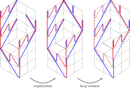
Figure 4: The process of exploration and loop erasion.

We start the induction with the trivial Toom cycle defined by $V:=\{0\}$ and $\psi(0)=(0,0)$. We identify a Toom cycle $\psi:\{0,\ldots,n-1\}\to{\mathbb{Z}}^{d+1}$ with the word $\psi(0)\cdots\psi(n-1)$. In each step of the induction, as long as (i) is not yet satisfied, we modify our Toom cycle according to the following two steps, which are illustrated in Figure 4.

• Exploration. We pick $k\in V_{\ast}$ such that $\displaystyle\mathchar 0\relax_{\psi(k)}\neq\mathchar 0\relax^{0}$ and $\psi_{d+1}(k)=T+1$, or if such a $k$ does not exist, with $\psi_{d+1}(k)=T$. We define $w_{s}$ by $\vec{H}_{s,{\rm out}}(\psi(k)):=(\psi(k),w_{s})$ $(s=1,2)$. In the word $\psi(0)\cdots\psi(n-1)$, on the place of $\psi(k)$, we insert the word $\psi(k)w_{1}\psi(k)w_{2}\psi(k)$.

• Loop erasion. If as a result of the exploration, there are $k_{1},k_{2}\in V_{\ast}$ with $k_{1}<k_{2}$ such that $\psi(k_{1})=\psi(k_{2})$, then we remove the subword $\psi(k_{1})\cdots\psi(k_{2})$ from the word $\psi(0)\cdots\psi(n-1)$ and on its place insert $\psi(k_{1})$. We repeat this step until $\psi(k_{1})\neq\psi(k_{2})$ for all $k_{1},k_{2}\in V_{\ast}$ with $k_{1}\neq k_{2}$.

The effect of the exploration step is that one sink is replaced by a source and two internal vertices, one of each charge, and than two new sinks are created (see Figure 4). These new sinks are created at height $-T$ or $-T+1$ and hence can overlap with each other or with other preexisting sinks, but not with sources or internal vertices. If the exploration step has created overlapping sinks or the two new internal vertices overlap, then these are removed in the loop erasion step. After the removal of a loop, all remaining vertices are of the same type (sink, source, or internal vertex of a given charge) as before. Using these observations, it is easy to check that:

• After exploration and loop erasion, the modified word $\psi$ is again a Toom cycle rooted at $(0,0)$ (see Definition 30) and the induction hypotheses (i)’, (ii), (iiia), (iiib), (iva), (ivb) and (vi) remain true.

Let $\Delta:=\{\psi(k):k\in V_{\ast},\ \mathchar 0\relax_{\psi(k)}\neq\mathchar 0\relax_{0}\}$. In each step of the induction, we remove one element from $\Delta$ with a given time coordinate, say $t$, and possibly add one or two new elements to $\Delta$ with time coordinates $t-1$. Since the explanation graph is finite, this cannot go on forever so the induction terminates after a finite number of steps. This completes the proof that Theorem 28 can be strengthened in the sense that the Toom contour $(V,{\cal E},v_{\circ},\psi)$ also satisfies condition (v) of Definition 8.

 

3.6 Forks

We recall that for Toom contours with two charges, Theorem 9 strengthened Theorem 7 by showing the presence of a Toom contour with certain additional properties. As we have seen in Subsection 2.4, such additional properties reduce the number of Toom contours one has to consider and hence lead to sharper Peierls bounds. In the present subsection, we will prove similar (but weaker) strengthened version of Theorem 7 that holds for an arbitrary number of charges.

Let $(V,{\cal E},v_{\circ},\psi)$ be a Toom contour. By definition, a fork is a source $v\in V_{\circ}$ such that:

$$\big{|}\{\psi(w):(v,w)\in\vec{E}\}\big{|}=2.$$ (3.23)

As we will show in a moment, the proof of Theorem 28 actually yields the following somewhat stronger statement. In the original formulation of Toom [Too80], his contours contain no sources but they contain objects that Toom calls forks and that effectively coincide with our usage of this term. For Toom, the fact that the number of sinks equals the number of forks plus one was part of his definition of a contour. In our formulation, this is a consequence of the fact that the number of sources equals the number of sinks.

Theorem 32 (Toom contour with forks only)

Theorem 28 can be strengthened in the sense that all sources $v\in V\backslash\{v_{\circ}\}$ are forks.

Proof Let us say that $v\in V_{\circ}$ is a point source if $|\{\psi(w):(v,w)\in\vec{E}\}|=1$. We first show that Theorem 28 can be strengthened in the sense that all sources $v\in V\backslash\{v_{\circ}\}$ are forks or point sources. Indeed, this is a direct consequence of the fact that the tight polars $(a_{i,1},\ldots,a_{i,\sigma})$ $(2\leq i\leq M)$ constructed in the proof of Lemma 27 are either point polars or have the property that the set $\{a_{i,s}:1\leq s\leq\sigma\}$ has precisely two elements. The latter give rise to forks while the former give rise to point sources or isolated vertices. Since a Toom countour is connected, sources other than the root can never be isolated vertices. This shows that Theorem 28 can be strengthened in the sense that all sources $v\in V\backslash\{v_{\circ}\}$ are forks or point sources.

Now if some $v\in V_{\circ}\backslash\{v_{\circ}\}$ is a point source, then we can simplify the Toom contour by removing this source from the contour and joining all elements of $\{w:(v,w)\in\vec{E}\}$ into a new source, that is embedded at the space-time point $z\in{\mathbb{Z}}^{d+1}$ defined by $\{z\}:=\{\psi(w):(v,w)\in\vec{E}\}$. Repeating this process until it is no longer possible to do so we arrive at Toom contour $(V,{\cal E},v_{\circ},\psi)$ with the additional property that all sources $v\in V\backslash\{v_{\circ}\}$ are forks.  

4 Bounds for eroders

Outline

In this section, we apply the abstract theory developed in the previous section to concrete models. In Subsection 4.1, we discuss the erosion criteria (1.9) and (2.12). In particular, we prove Lemma 10 and show that (2.12) implies that $\mathchar 0\relax$ is an eroder. In Subsection 4.2, we prove Lemmas 14 and 17 which give an exponential upper bound on the number of Toom contours and Toom cycles with a given number of edges. In Subsection 4.3, we prove Lemma 19 which shows that for eroders, finiteness of the Peierls sum is sufficient to conclude that $\overline{\rho}(p)>0$. At this point, we have proved all ingredients needed for the proof of Toom’s stability theorem described in Subsection 2.2 and also for the explicit bounds for concrete eroders stated in Subsection 2.4.

4.1 Eroders

In this subsection we prove Lemma 10. Our proof depends on the equivalence of (1.9) and the eroder property, which is proved in [Pon13, Thm 1]. In Lemma 33, we give an alternative direct proof that (2.12) implies that $\mathchar 0\relax$ is an eroder. Although we do not really need this alternative proof, we have included it since it is short and instructive. In particular, it links the eroder property to edge speeds, which we otherwise do not discuss but which are an important motivating idea behind the definition of Toom contours.

Proof of Lemma 10 In [Pon13, Lemma 12] it is shown that (1.9) is equivalent to the existence of a polar function $L$ of dimension $2\leq\sigma\leq d+1$ and constants $\varepsilon_{1},\ldots,\varepsilon_{\sigma}$ such that $\sum_{s=1}^{\sigma}\varepsilon_{s}>0$ and for each $1\leq s\leq\sigma$, there exists an $A_{s}\in{\cal A}(\mathchar 0\relax)$ such that $\varepsilon_{s}-L_{s}(i)\leq 0$ for all $i\in A_{s}$. It follows that

$$\sum_{s=1}^{\sigma}\sup_{A\in{\cal A}(\mathchar 0\relax)}\inf_{i\in A}L_{s}(i)\geq\sum_{s=1}^{\sigma}\inf_{i\in A_{s}}L_{s}(i)\geq\sum_{s=1}^{\sigma}\varepsilon_{s}>0,$$ (4.1)

which shows that (2.12) holds. Assume, conversely, that (2.12) holds. Since ${\cal A}(\mathchar 0\relax)$ is finite, for each $1\leq s\leq\sigma$ we can choose $A_{s}(\mathchar 0\relax)\in{\cal A}(\mathchar 0\relax)$ such that

$$\varepsilon_{s}:=\inf_{i\in A_{s}(\mathchar 0\relax)}L_{s}(i)=\sup_{A\in{\cal A}(\mathchar 0\relax)}\inf_{i\in A}L_{s}(i).$$ (4.2)

Then (2.12) says that $\sum_{s=1}^{\sigma}\varepsilon_{s}>0$. Let $H_{s}:=\{z\in{\mathbb{R}}^{d}:L_{s}(z)\geq\varepsilon_{s}\}$. By the definition of a polar function, $\sum_{s=1}^{\sigma}L_{s}(z)=0$ for each $z\in{\mathbb{R}}^{d}$, and hence the condition $\sum_{s=1}^{\sigma}\varepsilon_{s}>0$ implies that for each $z\in{\mathbb{R}}^{d}$, there exists an $1\leq s\leq\sigma$ such that $L_{s}(z)<\varepsilon_{s}$. In other words, this says that $\bigcap_{s=1}^{\sigma}H_{s}=\emptyset$. For each $1\leq s\leq\sigma$, the set $A_{s}(\mathchar 0\relax)$ is contained in the half-space $H_{s}$ and hence the same is true for ${\rm Conv}(A_{s}(\mathchar 0\relax))$, so we conclude that

$$\bigcap_{s=1}^{\sigma}{\rm Conv}\big{(}A_{s}(\mathchar 0\relax)\big{)}=\emptyset,$$ (4.3)

from which (1.9) follows.  

Lemma 33 (The eroder property)

If a non-constant monotonic function $\mathchar 0\relax:\{0,1\}^{{\mathbb{Z}}^{d}}\to\{0,1\}$ satisfies (2.12), then $\mathchar 0\relax$ is an eroder.

Proof Most of the argument has already been given below Lemma 10. It only remains to prove (2.14). It suffices to prove the claim for $n=1$; the general claim then follows by induction. Assume that $i\in{\mathbb{Z}}^{d}$ satisfies $L_{s}(i)>r_{s}(X^{0}_{0})-\delta_{s}$. We need to show that $X^{0}_{1}(i)=1$ for all such $i$. By the definition of $\delta_{s}$, we can choose $A\in{\cal A}(\mathchar 0\relax)$ such that $\inf_{j\in A}L_{s}(j)=\delta_{s}$. It follows that $L_{s}(i+j)>r_{s}(X^{0}_{0})$ for all $j\in A$ and hence $X^{0}_{0}(i+j)=1$ for all $j\in A$, which implies $X^{0}_{1}(i)=1$ by (1.8).  

4.2 Exponential bounds on the number of contours

In this subsection, we prove Lemmas 14 and 17.

Proof of Lemma 14 We first consider the case that the number of charges $\sigma$ is even. Let $T=(V,{\cal E},v_{\circ},\psi)\in{\cal T}^{\prime}_{0}$. Recall that $(V,{\cal E})$ is a directed graph with $\sigma$ types of edges, that are called charges. In $(V,{\cal E})$, all edges point in the direction from the sources to the sinks. We modify $(V,{\cal E})$ by reversing the direction of edges of the charges ${\textstyle\frac{{1}}{{2}}}\sigma+1,\ldots,\sigma$. Let $(V,{\cal E}^{\prime})$ denote the modified graph. In $(V,{\cal E}^{\prime})$, the number of incoming edges at each vertex equals the number of outgoing edges. Since moreover the undirected graph $(V,E)$ is connected, it is not hard to see that it is possible to walk through the directed graph $(V,{\cal E}^{\prime})$ starting from the root using an edge of charge $1$, in such a way that each directed edge of ${\cal E}^{\prime}$ is traversed exactly once.

Let $m:=\sigma n_{\rm e}(T)$ denote the total number of edges of $(V,{\cal E}^{\prime})$ and for $0<k\leq m$, let $(v_{k-1},v_{k})\in\vec{E}^{\prime}_{s_{k}}$ denote the $k$-th step of the walk, which has charge $s_{k}$. Let $\delta_{k}:=\vec{\psi}(v_{k})-\vec{\psi}(v_{k-1})$ denote the spatial increment of the $k$-th step. Note that the temporal increment is determined by the charge $s_{k}$ of the $k$-th step. Let $k_{0},\ldots,k_{\sigma/2}$ denote the times when the walk visits the root $v_{\circ}$. We claim that in order to specify $(V,{\cal E},v_{\circ},\psi)$ uniquely up to equivalence, in the sense defined in (2.7), it suffices to know the sequences

$$(s_{1},\ldots,s_{m}),\quad(\delta_{1},\ldots,\delta_{m}),\quad\mbox{and}\quad(k_{0},\ldots,k_{\sigma/2}).$$ (4.4)

Indeed, the sinks and sources correspond to changes in the temporal direction of the walk which can be read off from the charges. Although the images under $\psi$ of sources may overlap, we can identify which edges connect to the root, and since we also know the increment of $\psi(v_{k})$ in each step, all objects in (2.7) can be identified.

The first charge $s_{1}$ is 1 and after that, in each step, we have the choice to either continue with the same charge or choose one of the other ${\textstyle\frac{{1}}{{2}}}\sigma$ available charges. This means that there are no more than $({\textstyle\frac{{1}}{{2}}}\sigma+1)^{m-1}$ possible ways to specify the charges $(s_{1},\ldots,s_{m})$. Setting $M:=\big{|}\bigcup_{s=1}^{\sigma}A_{s}(\mathchar 0\relax)\big{|}$, we see that there are no more than $M^{m}$ possible ways to specify the spatial increments $(\delta_{1},\ldots,\delta_{m})$. Since $k_{0}=0,k_{\sigma/2}=m$, we can roughly estimate the number of ways to specify the visits to the root from above by $n^{\sigma/2-1}$. Recalling that $m=\sigma n_{\rm e}(T)$, this yields the bound

$$N_{n}\leq n^{\sigma/2-1}({\textstyle\frac{{1}}{{2}}}\sigma+1)^{\sigma n-1}M^{\sigma n}.$$ (4.5)

This completes the proof when $\sigma$ is even.

When $\sigma$ is odd, we modify $(V,{\cal E})$ by doubling all edges of charge $\sigma$, i.e., we define $(V,{\cal F})$ with

$${\cal F}=(\vec{F}_{1},\ldots,\vec{F}_{\sigma+1}):=(\vec{E}_{1},\ldots,\vec{E}_{\sigma},\vec{E}_{\sigma}),$$ (4.6)

and next we modify $(V,{\cal F})$ by reversing the direction of all edges of the charges $\lceil{\textstyle\frac{{1}}{{2}}}\sigma\rceil+1,\ldots,\sigma+1$. We can define a walk in the resulting graph $(V,{\cal F}^{\prime})$ as before and record the charges and spatial increments for each step, as well as the visits to the root. In fact, in order to specify $(V,{\cal E},v_{\circ},\psi)$ uniquely up to equivalence, we do not have to distinguish the charges $\sigma$ and $\sigma+1$. Recall that edges of the charges $\sigma$ and $\sigma+1$ result from doubling the edges of charge $\sigma$ and hence always come in pairs, connecting the same vertices. Since sinks do not overlap and since internal vertices of a given charge do not overlap, and since we traverse edges of the charges $\sigma$ and $\sigma+1$ in the direction from the sinks towards the sources, whenever we are about to traverse an edge that belongs to a pair of edges of the charges $\sigma$ and $\sigma+1$, we know whether we have already traversed the other edge of the pair. In view of this, for each pair, we only have to specify the spatial displacement at the first time that we traverse an edge of the pair. Using these considerations, we arrive at the bound

$$N_{n}\leq n^{\lceil\sigma/2\rceil-1}(\lceil{\textstyle\frac{{1}}{{2}}}\sigma\rceil+1)^{(\sigma+1)n-1}M^{\sigma n}.$$ (4.7)

 

Proof of Lemma 17 The proof goes along the same lines as that of Lemma 14 for the case $\sigma$ is even. Observe that for $\sigma=2$, the walk visits the root 0 twice: $k_{0}=0,k_{1}=m$. Thus $(k_{0},k_{1})$ is deterministic, and we only need to specify the sequences

$$(s_{1},\ldots,s_{m}),\quad(\delta_{1},\ldots,\delta_{m}).$$ (4.8)

The first charge $s_{1}$ is 1 and after that, in each step, we have the choice to either continue with the same charge or choose charge 2. This means that there are no more than $2^{m-1}$ possible ways to specify the charges $(s_{1},\ldots,s_{m})$. Once we have done that, by condition (v) of Definition 8 of what it means for a cycle to be strongly present, we know for each $0<k\leq m$ whether the spatial increment $\delta_{k}$ is in $A_{1}(\mathchar 0\relax)$ or $A_{2}(\mathchar 0\relax)$. Setting $M_{s}:=|A_{s}(\mathchar 0\relax)\big{|}$ $(s=1,2)$, using the fact that $|\vec{E}_{1}|=|\vec{E}_{2}|=2n_{\rm e}(T)=m/2$, we see that there are no more than $M_{1}^{m/2}\cdot M_{2}^{m/2}$ possible ways to specify $(\delta_{1},\ldots,\delta_{m})$. This yields the bound

$$N_{n}\leq 2^{2n-1}M_{1}^{n}\cdot M_{2}^{n}.$$ (4.9)

 

4.3 Finiteness of the Peierls sum

In this subsection, we prove Proposition 18 about the presence of a large contour. As a direct consequece of this proposition, we obtain Lemma 19 which says that for an eroder, finiteness of the Peierls sum in (2.25) suffices to conclude that the intensity of the upper invariant law is positive. We also prove a stronger version of Proposition 18, where we show the strong presence of a Toom contour in which all sources are forks.

Proof of Proposition 18 Recall the definition of the modified collection of monotonic maps ${\bm{\mathchar 0\relax}}^{(r)}$ in (2.32). Let $\overline{x}^{(r)}$ denote the maximal trajectory of ${\bm{\mathchar 0\relax}}^{(r)}$. For each integer $q\geq 0$, let $C_{q}:={\rm Conv}(\{qj_{1},\ldots,qj_{\sigma}\})$. Then

$$C_{q+1}=\big{\{}i+j_{s}:i\in C_{q},\ 1\leq s\leq\sigma\big{\}}\qquad(q\geq 0).$$ (4.10)

Using this, it is easy to see by induction that our assumption that $\overline{x}^{(r)}_{-r}(i)=0$ for all $i\in C_{r}$ implies that $\overline{x}^{(r)}_{-q}(i)=0$ for all $i\in C_{q}$ and $0\leq q\leq r$. In particular, this holds for $q=0$, so $\overline{x}^{(r)}_{0}(0)=0$.

Using this, it is straightforward to adapt the proof of Lemma 22 and show that there is an explanation graph $(U,{\cal H})$ for $(0,0)$ present in ${\bm{\mathchar 0\relax}}^{(r)}$ which has the additional properties:

• $\big{\{}i\in{\mathbb{Z}}^{d}:(i,-q)\in U\big{\}}=C_{q}$ $(0\leq q\leq r)$,

• $\big{(}(i,-q),(i+j_{s},-q-1)\big{)}\in\vec{H}_{s}$ $(0\leq q<r,\ i\in C_{q})$.

In particular, these properties imply that

• $t\leq-r$ for all $(i,t)\in U_{\ast}$.

Theorem 28 tells us that there is a Toom contour $(V,{\cal E},v_{\circ},\psi)$ rooted at $(0,0)$ present in ${\bm{\mathchar 0\relax}}^{(r)}$ with the additional properties that $\psi(V)\subset U$, $\psi(V_{\ast})\subset U_{\ast}$, and $\psi(\vec{E}_{s})\subset\psi(\vec{H}_{s})$ for all $1\leq s\leq\sigma$. This immediately implies that $\psi_{d+1}(v)\leq-r$ for all $v\in V_{\ast}$.

To see that the Toom contour can be chosen such that moreover $\psi_{d+1}(v)\leq 1-r$ for all $v\in V_{\circ}\backslash\{v_{\circ}\}$, we have to look into the proof of Theorem 28. In Subsection 3.3 we defined an equivalence relation $\sim$ on the set of vertices $U$ of an explanation graph $(U,{\cal H})$. In Lemma 25, we showed that the set of all equivalence classes has the structure of a directed tree. If we draw time downwards, then the root of this tree lies below. In the proof of Proposition 24, we constructed a Toom matching for $(U,{\cal H})$ with the property that except for the root, all other polars lie at a level above the last level where the tree still consisted of a single equivalence class. Finally, in the proof of Theorem 28, we used these polars to construct sources that lie at most one level below the corresponding polar. The upshot of all of this is that in order to show that $\psi_{d+1}(v)\leq 1-r$ for all $v\in V_{\circ}\backslash\{v_{\circ}\}$, it suffices to show that the set of vertices $\{(i,t)\in U:t=1-r\}$ forms a single equivalence class as defined in Subsection 3.3.

To see that this indeed is the case, call two points $i=(i_{1},\dots,i_{\sigma}),j=(j_{1},\dots,j_{\sigma})\in C_{r-1}$ neighbours if there exist $1\leq s_{1},s_{2}\leq\sigma$ with $s_{1}\neq s_{2}$ such that $i_{s_{1}}=j_{s_{1}}-1$, $i_{s_{2}}=j_{s_{2}}+1$, and $i_{s}=j_{s}$ for all $s\in\{1,\ldots,\sigma\}\backslash\{s_{1},s_{2}\}$. Define $k\in C_{r}$ by $k_{s_{1}}=j_{s_{1}}$, $k_{s_{2}}=j_{s_{2}}+1$, and $k_{s}=j_{s}$ for all other $s$. Then $\big{(}(i,1-r),(k,-r)\big{)}\in\vec{H}$ and $\big{(}(j,1-r),(k,-r)\big{)}\in\vec{H}$ which proves that $(i,1-r)\approx(j,1-r)$. Since any two points in $C_{r-1}$ are connected by a path that in each step moves from a point to a neighbouring point, this shows that $\{(i,t)\in U:t=1-r\}$ forms a single equivalence class.

To complete the proof, we need to show that if $\sigma=2$, then we can construct the Toom contour so that in addition it is strongly present in ${\bm{\mathchar 0\relax}}^{(r)}$. We use the same explanation graph $(U,{\cal H})$ for $(0,0)$ with properties (i)–(iii) as above. Theorem 29 now tells us that there is a Toom contour $(V,{\cal E},v_{\circ},\psi)$ rooted at $(0,0)$ strongly present in ${\bm{\mathchar 0\relax}}^{(r)}$ with the additional properties that $\psi(V)\subset U$, $\psi(V_{\ast})\subset U_{\ast}$, and $\psi(\vec{E}_{s})\subset\psi(\vec{H}_{s})$ for all $1\leq s\leq\sigma$. This again immediately implies that $\psi_{d+1}(v)\leq-r$ for all $v\in V_{\ast}$, so again it remains to show that the Toom contour can be chosen such that moreover $\psi_{d+1}(v)\leq 1-r$ for all $v\in V_{\circ}\backslash\{v_{\circ}\}$.

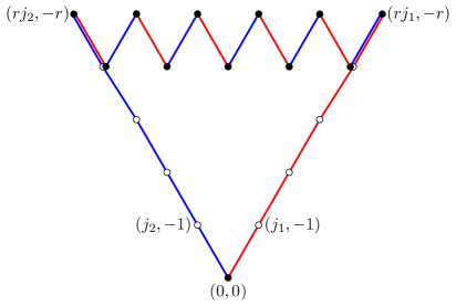
Figure 5: The Toom cycle $\psi$ described in the proof of Proposition 18.

To see that this is the case, we have to look into the proof of Theorem 29. Instead of starting the inductive construction with the trivial Toom cycle of length zero, we claim that it is possible to start with a Toom cycle $\psi$ of length $4r$ for which all sources except the root have the time coordinate $1-r$ and all sinks have the time coordinate $-r$. Since the process of exploration and loop erasion will then only create new sources with time coordinate $-r$ or lower, the claim then follows. A Toom cycle $\psi$ with the described properties is drawn in Figure 5. More formally, this cycle has the following description. Starting from $(0,0)$, it first visits the points $(-k,kj_{1})$ with $k=1,\ldots,r$. Next, it alternatively visits the points $(1-r,(r-k)j_{1}+(k-1)j_{2})$ and $(-r,(r-k)j_{1}+kj_{2})$ with $k=1,\ldots,r$. Finally, it visits the points $(k-r,(r-k)j_{2})$ with $k=1,\ldots,r$, ending in $(0,0)$, where it started.  

Proposition 34 (Large contours with forks only)

Proposition 18 can be strengthened in the sense that all sources $v\in V\backslash\{v_{\circ}\}$ are forks.

Proof A Toom contours with two charges that is strongly present in $\Phi^{(r)}$ automatically has the property that all sources $v\in V\backslash\{v_{\circ}\}$ are forks, because of condition (vi) of Definition 8. Thus, it suffices to prove the claim for Toom contours with three or more charges. In this case, as pointed out in the proof of Proposition 18, the fact that all sources $v\in V\backslash\{v_{\circ}\}$ are forks is an automatic result of the construction used in the proof of Theorem 28. Since we used this same construction in the proof of Proposition 18, the contour constructed there also has this property.  

Proof of Lemma 19 Let

$${\cal T}^{\prime}_{0,r}:=\big{\{}(V,{\cal E},v_{\circ},\psi)\in{\cal T}^{\prime}_{0}:\psi_{d+1}(v)\leq-r\mbox{ for all }v\in V_{\ast}\big{\}}.$$ (4.11)

By assumption, $\displaystyle\sum_{T\in{\cal T}^{\prime}_{0}}p^{n_{\ast}(T)}<\infty$, so we can choose $r$ sufficiently large such that

$$\varepsilon:=\sum_{T\in{\cal T}^{\prime}_{0,r}}p^{n_{\ast}(T)}<1.$$ (4.12)

Fix $j_{s}\in A_{s}(\mathchar 0\relax)$ $(1\leq s\leq\sigma)$ and set $\Delta_{r}:={\mathbb{Z}}^{d}\cap{\rm Conv}(\{rj_{1},\ldots,rj_{\sigma}\})$. Then Proposition 18 allows us to estimate

$${\mathbb{P}}\big{[}\overline{X}_{-r}(i)=0\ \forall i\in\Delta_{r}\big{]}\leq\sum_{T\in{\cal T}^{\prime}_{0,r}}{\mathbb{P}}\big{[}T\mbox{ is present in }\Phi^{(r)}\big{]}\leq\varepsilon,$$ (4.13)

where in the last step we have used that $\psi_{d+1}(v)\leq-r$ for all $v\in V_{\ast}$ and hence all sinks of $V$ must be mapped to space-time points $(i,t)$ where $\Phi^{(r)}_{(i,t)}=\Phi_{(i,t)}$. By translation invariance,

$${\mathbb{P}}\big{[}\overline{X}_{-r}(i)=1\mbox{ for some }i\in\Delta_{r}\big{]}\leq\sum_{i\in\Delta_{r}}{\mathbb{P}}\big{[}\overline{X}_{-r}(i)=1\big{]}=|\Delta_{r}|{\mathbb{P}}\big{[}\overline{X}_{0}(0)=1\big{]}.$$ (4.14)

Combining this with our previous formulas, we see that

$$\overline{\rho}(p)={\mathbb{P}}\big{[}\overline{X}_{0}(0)=1\big{]}\geq|\Delta_{r}|^{-1}(1-\varepsilon)>0.$$ (4.15)

For Toom contours with two charges, Proposition 18 guarantees the strong presence of a large Toom contour, so we can argue similarly, replacing ${\cal T}^{\prime}_{0}$ by ${\cal T}^{\prime\prime}_{0}$.  

Remark In Peierls arguments, it is frequently extremely helpful to be able to draw conclusions based only on the fact that that the Peierls sum is finite (but not necessarily less than one). These sorts of arguments played an important role in [KSS14], where we took inspiration for Lemma 19, and can be traced back at least to [Dur88, Section 6a].

5 Cooperative branching and the identity map

In this subsection, we study the monotone random cellular automaton that applies the maps $\mathchar 0\relax^{0},\mathchar 0\relax^{\rm id}$, and $\mathchar 0\relax^{\rm coop,d}$ with probabilities $p,q,r$, respectively. For each $p,r\geq 0$ such that $p+r\leq 1$, let $\overline{\rho}(p,r)$ denote the intensity of the upper invariant law of the process with parameters $p,1-p-r,r$. For each $0\leq r<1$, there exists a $p_{\rm c}(r)\in[0,1-r]$ such that $\overline{\rho}(p,r)>0$ for $0\leq p<p_{\rm c}(r)$ and $\overline{\rho}(p,r)=0$ for $p_{\rm c}(r)<p\leq 1-r$. We give lower bounds on $p_{\rm c}(r)$.

Recall from Subsection 2.5 that we set $\sigma=2$ and for the sets $A_{s}(\mathchar 0\relax_{k})$ in (2.9) we make the choices

$$\begin{array}[]{ll}\displaystyle A_{1}(\mathchar 0\relax^{\rm id}):=A_{1},&A_{2}(\mathchar 0\relax^{\rm id}):=A_{1},\\[5.0pt] \displaystyle A_{1}(\mathchar 0\relax^{\rm coop,d}):=A_{1},&A_{2}(\mathchar 0\relax^{\rm coop,d}):=A_{2},\end{array}$$ (5.1)

with $A_{1}:=\{0\}$ and $A_{2}:=\{e_{1},\dots,e_{d}\}$. Let $\Phi=(\Phi_{(i,t)})_{(i,t)\in{\mathbb{Z}}^{3}}$ be an i.i.d. collection of monotonic maps so that ${\mathbb{P}}[\Phi_{(i,t)}=\mathchar 0\relax^{0}]=p$, ${\mathbb{P}}[\Phi_{(i,t)}=\mathchar 0\relax^{\rm id}]=q$, and ${\mathbb{P}}[\Phi_{(i,t)}=\mathchar 0\relax^{\rm coop,d}]=r$. We let ${\cal T}_{0}$ denote the set of Toom contours $(V,\mathcal{E},0,\psi)$ rooted at the origin with respect to the given choice of $\sigma$ and the sets $A_{s}(\mathchar 0\relax_{k})$ in (2.47). Theorem 7 then implies the Peierls bound

$$1-\overline{\rho}\leq\sum_{T\in{\cal T}_{0}}{\mathbb{P}}\big{[}T\mbox{ is strongly present in }\Phi\big{]}.$$ (5.2)

In the remainder of this section, we give an upper bound on this expression.

Recall from Subsection 3.5 that if we reverse the direction of edges of charge 2, then the Toom graph becomes a directed cycle with edge set $\vec{E}_{1}\cup{\mathchoice{\vbox{\offinterlineskip\halign{#\cr\reflectbox{$\displaystyle\vec{}\mkern 4.0mu$}\cr\kern-4.30554pt\cr$\displaystyle E$\cr}}}{\vbox{\offinterlineskip\halign{#\cr\reflectbox{$\textstyle\vec{}\mkern 4.0mu$}\cr\kern-4.30554pt\cr$\textstyle E$\cr}}}{\vbox{\offinterlineskip\halign{#\cr\reflectbox{$\scriptstyle\vec{}\mkern 4.0mu$}\cr\kern-3.01389pt\cr$\scriptstyle E$\cr}}}{\vbox{\offinterlineskip\halign{#\cr\reflectbox{$\scriptscriptstyle\vec{}\mkern 4.0mu$}\cr\kern-2.15277pt\cr$\scriptscriptstyle E$\cr}}}}_{2}$. For any set $A\subset{\mathbb{Z}}^{d}$, let us write $-A:=\{-i:i\in A\}$. For any $(v,w)\in\vec{E}_{1}\cup{\mathchoice{\vbox{\offinterlineskip\halign{#\cr\reflectbox{$\displaystyle\vec{}\mkern 4.0mu$}\cr\kern-4.30554pt\cr$\displaystyle E$\cr}}}{\vbox{\offinterlineskip\halign{#\cr\reflectbox{$\textstyle\vec{}\mkern 4.0mu$}\cr\kern-4.30554pt\cr$\textstyle E$\cr}}}{\vbox{\offinterlineskip\halign{#\cr\reflectbox{$\scriptstyle\vec{}\mkern 4.0mu$}\cr\kern-3.01389pt\cr$\scriptstyle E$\cr}}}{\vbox{\offinterlineskip\halign{#\cr\reflectbox{$\scriptscriptstyle\vec{}\mkern 4.0mu$}\cr\kern-2.15277pt\cr$\scriptscriptstyle E$\cr}}}}_{2}$ we say that $\psi\big{(}(v,w)\big{)}$ is

1. outward, if $\psi_{3}(w)=\psi_{3}(v)-1$ and $\vec{\psi}(w)-\vec{\psi}(v)\in A_{2}$,

2. upward, if $\psi_{3}(w)=\psi_{3}(v)-1$ and $\vec{\psi}(w)-\vec{\psi}(v)\in A_{1}$,

3. inward, if $\psi_{3}(w)=\psi_{3}(v)+1$ and $\vec{\psi}(w)-\vec{\psi}(v)\in-A_{2}$,

4. downward, if $\psi_{3}(w)=\psi_{3}(v)+1$ and $\vec{\psi}(w)-\vec{\psi}(v)\in-A_{1}$.

The use of the words “upward” and “downward” are inspired by our habit of drawing negative time upwards in pictures. As $|A_{2}|=d$, we distinguish $d$ types of outward and inward edges: we say that $\psi\big{(}(v,w)\big{)}$ is type $i$, if $|\vec{\psi}(w)-\vec{\psi}(v)|=e_{i}$. Our definitions in (5.1) together with Definitions 6 and 8 imply that a Toom contour is strongly present in $\Phi$ if and only if the following conditions are satisfied:

• $\displaystyle\Phi_{\psi(v)}=\mathchar 0\relax^{0}$ for all $\displaystyle v\in V_{\ast}$,

• $\displaystyle\Phi_{\psi(v)}\in\{\mathchar 0\relax^{\rm id},\mathchar 0\relax^{\rm coop,d}\}$ for all $\displaystyle v\in V_{1}\cup V_{2}\cup\{v_{\circ}\}$,

• $\displaystyle\Phi_{\psi(v)}=\mathchar 0\relax^{\rm coop,d}$ for all $\displaystyle v\in V_{\circ}\backslash\{v_{\circ}\}$,

• If $(v,w)\in\vec{E}^{\ast}_{1}$, then $\psi\big{(}(v,w)\big{)}$ is upward,

• If $(v,w)\in{\mathchoice{\vbox{\offinterlineskip\halign{#\cr\reflectbox{$\displaystyle\vec{}\mkern 4.0mu$}\cr\kern-4.30554pt\cr$\displaystyle E$\cr}}}{\vbox{\offinterlineskip\halign{#\cr\reflectbox{$\textstyle\vec{}\mkern 4.0mu$}\cr\kern-4.30554pt\cr$\textstyle E$\cr}}}{\vbox{\offinterlineskip\halign{#\cr\reflectbox{$\scriptstyle\vec{}\mkern 4.0mu$}\cr\kern-3.01389pt\cr$\scriptstyle E$\cr}}}{\vbox{\offinterlineskip\halign{#\cr\reflectbox{$\scriptscriptstyle\vec{}\mkern 4.0mu$}\cr\kern-2.15277pt\cr$\scriptscriptstyle E$\cr}}}}^{\ast}_{2}$, then $\displaystyle\left\{\begin{array}[]{ll}\psi\big{(}(v,w)\big{)}\mbox{ is downward }\quad\mbox{if }\Phi_{\psi(w)}=\mathchar 0\relax^{\rm id},\\ \psi\big{(}(v,w)\big{)}\mbox{ is inward }\quad\mbox{if }\Phi_{\psi(w)}=\mathchar 0\relax^{\rm coop,d},\end{array}\right.$

• If $(v,w)\in\vec{E}^{\circ}_{1}$, then $\psi\big{(}(v,w)\big{)}$ is outward,

• If $(v,w)\in{\mathchoice{\vbox{\offinterlineskip\halign{#\cr\reflectbox{$\displaystyle\vec{}\mkern 4.0mu$}\cr\kern-4.30554pt\cr$\displaystyle E$\cr}}}{\vbox{\offinterlineskip\halign{#\cr\reflectbox{$\textstyle\vec{}\mkern 4.0mu$}\cr\kern-4.30554pt\cr$\textstyle E$\cr}}}{\vbox{\offinterlineskip\halign{#\cr\reflectbox{$\scriptstyle\vec{}\mkern 4.0mu$}\cr\kern-3.01389pt\cr$\scriptstyle E$\cr}}}{\vbox{\offinterlineskip\halign{#\cr\reflectbox{$\scriptscriptstyle\vec{}\mkern 4.0mu$}\cr\kern-2.15277pt\cr$\scriptscriptstyle E$\cr}}}}^{\circ}_{2}$, then $\psi\big{(}(v,w)\big{)}$ is downward,

where $\vec{E}^{\circ}_{i}$ and $\vec{E}^{\ast}_{i}$ are defined in (2.5). If $(V,{\cal E},v_{\circ},\psi)$ is a Toom contour rooted at 0 that is strongly present in $\Phi$, then we can fully specify $\psi$ by saying for each $(v,w)\in\vec{E}_{1}\cup{\mathchoice{\vbox{\offinterlineskip\halign{#\cr\reflectbox{$\displaystyle\vec{}\mkern 4.0mu$}\cr\kern-4.30554pt\cr$\displaystyle E$\cr}}}{\vbox{\offinterlineskip\halign{#\cr\reflectbox{$\textstyle\vec{}\mkern 4.0mu$}\cr\kern-4.30554pt\cr$\textstyle E$\cr}}}{\vbox{\offinterlineskip\halign{#\cr\reflectbox{$\scriptstyle\vec{}\mkern 4.0mu$}\cr\kern-3.01389pt\cr$\scriptstyle E$\cr}}}{\vbox{\offinterlineskip\halign{#\cr\reflectbox{$\scriptscriptstyle\vec{}\mkern 4.0mu$}\cr\kern-2.15277pt\cr$\scriptscriptstyle E$\cr}}}}_{2}$ whether $\psi\big{(}(v,w)\big{)}$ is upward, downward, inward or outward, and its type in the latter two cases. In other words, we can represent the contour by a word of length $n$ consisting of the letters from the alphabet $\{o_{1},\dots,o_{d},u,d,i_{1},\dots,i_{d}\}$, which represents the different kinds of steps the cycle can take. Then we obtain a word consisting of the letters $o_{1},\dots,o_{d},u,d,i_{1},\dots,i_{d}$ that must satisfy the following rules:

• Each outward step must be immediately preceded by a downward step.

• Between two occurrences of the string $do_{\cdot}$, and also before the first occurrence of $do_{\cdot}$ and after the last occurrence, we first see a string consisting of the letter $u$ of length $\geq 0$, followed by a string consisting of the letters $d,i_{1},\dots,i_{d}$, again of length $\geq 0$.

So, for example the contour in the middle of Figure 3 is described by the following word:

$$\underbrace{uuuu}\underbrace{do_{1}}\underbrace{do_{1}}\underbrace{uu}\underbrace{do_{2}}\underbrace{do_{2}}\underbrace{di_{1}}\underbrace{di_{1}}\underbrace{do_{1}}\underbrace{do_{1}}\underbrace{di_{1}}\underbrace{di_{1}}\underbrace{di_{2}}\underbrace{di_{2}}.$$ (5.3)

We call a sequence of length $\geq 0$ of consecutive downward/upward steps a downward/upward segment. We can alternatively represent $\psi$ by a word of length $n$ consisting of the letters from $\{o_{1},\dots,o_{d},U,D,i_{1},\dots,i_{d},i^{\circ}_{1},\dots,i^{\circ}_{d}\}$, where $U$ and $D$ represent upward and downward segments. Let us for the moment ignore the $\circ$ superscripts. Then we can obtain a word consisting of these letters that must satisfy the following rules:

• Each outward step must be immediately preceded by a downward segment of length $\geq 1$ and followed by an upward segment of length $\geq 0$.

• The first step is an upward segment.

• Between two occurrences of the string $Do_{\cdot}U$, and also before the first and after the last occurrence, we see a sequence of the string $Di_{\cdot}$ of length $\geq 0$.

• The last step is a downward segment.

We add the superscript $\circ$ to each inward step whose endpoint overlaps with the image of a source other than the root already visited by the cycle in one of the previous steps. For any Toom contour $T$ denote by $W(T)$ the corresponding word satisfying these rules. The structure of such a representation of a contour becomes more clear if we indicate the vertices in $V_{1},V_{2},V_{\ast}$, and $V_{\circ}$ with the symbols $1,2,\ast,\circ$, respectively. Then the contour in the middle of Figure 3 is described by the following word:

$$\accentset{\circ}{|}U\accentset{\ast}{|}\underbrace{D\accentset{\circ}{|}o_{1}\accentset{1}{|}U}\accentset{\ast}{|}\underbrace{D\accentset{\circ}{|}o_{1}\accentset{1}{|}U}\accentset{\ast}{|}\underbrace{D\accentset{\circ}{|}o_{2}\accentset{1}{|}U}\accentset{\ast}{|}\underbrace{D\accentset{\circ}{|}o_{2}\accentset{1}{|}U}\accentset{\ast}{|}\underbrace{D\accentset{2}{|}i_{1}}\accentset{2}{|}\underbrace{D\accentset{2}{|}i_{1}}\accentset{2}{|}\underbrace{D\accentset{\circ}{|}o_{1}\accentset{1}{|}U}\accentset{\ast}{|}\underbrace{D\accentset{\circ}{|}o_{1}\accentset{1}{|}U}\accentset{\ast}{|}\underbrace{D\accentset{2}{|}i^{\circ}_{1}}\accentset{2}{|}\underbrace{D\accentset{2}{|}i_{1}}\accentset{2}{|}\underbrace{D\accentset{2}{|}i_{2}}\accentset{2}{|}\underbrace{D\accentset{2}{|}i_{2}}\accentset{2}{|}D\accentset{\circ}{|}.$$ (5.4)

Finally, let $l^{+}(T),l^{-}(T)$ and $l^{-,\circ}(T)$ denote the vectors containing the lengths of the upward segments, downward segments followed by $o_{\cdot}$ or $i_{\cdot}$ and downward segments followed by $i^{\circ}_{\cdot}$ respectively in the order we encounter them along the cycle. For the example above we have:

$$l^{+}(T)= (4,0,2,0,0,0,0),$$ (5.5)

$$l^{-}(T)= (1,1,1,1,0,0,1,1,0,0,0,0,0),$$

$$l^{-,\circ}(T)= (0).$$

Claim 1

Let $T$ be a Toom contour strongly present in $\Phi$ rooted at 0. Then $W(T),l^{+}(T)$ and $l^{-}(T)$ uniquely determine $(V,{\cal E},0,\psi)$.

Proof Knowing the word describing $T$ together with the lengths of all upward and downward segments uniquely determines the contour, so it is enough to show that $W(T),l^{+}(T)$ and $l^{-}(T)$ determines $l^{-,\circ}(T)=(l_{1},\dots,l_{j})$ $(j\geq 0)$.

Assume we know $l_{1},\dots,l_{i}$ for some $0\leq i<j$. We then know the length and type of each step along the cycle up to the downward segment corresponding to $l_{i+1}$, that is we know the coordinates of its starting point. This downward segment ends at a charge 2 internal vertex, and the consecutive step is inward ending at a source other than the root already visited by the cycle. The cycle enters each such source by a downward step and leaves it by an outward step, hence by the structure of the explanation graph the endpoints of this outward step must coincide with the endpoints of the inward step following the downward segment with length $l_{i+1}$. As each outward step is followed by an upward segment, the starting point of the consecutive upward segment must be the endpoint of our downward segment. The endpoint of every upward segment is a defective site, and each site along a downward segment (except maybe its endpoints) is an identity site, so this upward segment must contain every site of our downward segment. Furthermore, by (iii) of Definition 2 of an embedding there cannot be any other upward segment that overlaps with this downward segment. Therefore, given the starting coordinates of our downward segment, we check which upward segment visited these coordinates previously, and we let $l_{i+1}$ be the distance between the starting points of this upward segment and our downward segment.  

By a small abuse of notation, let us also use the letters $o,i$ to indicate the number of times the symbols $o,i$ occur in our representation of the contour (regardless of the sub- and superscripts). As our contour is a cycle starting and ending at 0, we must have the same number of inward and outward steps, furthermore, the total lengths of upward and downward segments must be equal as well:

$$o=i\quad\mbox{and}\quad\|l^{+}(T)\|_{1}=\|l^{-}(T)\|_{1}+\|l^{-,\circ}(T)\|_{1}.$$ (5.6)

We observe that each source (other than the root) is followed by an outward step, thus

$$|V_{\circ}|=|V_{\ast}|=i+1.$$ (5.7)

Finally, in the representation $W(T)$ of a contour the first and last step is $U$ and $D$ respectively, and in between $i$ strings of $DoU$ alternate with $i$ strings of $Di$. Thus, letting $0\leq j\leq i$ denote the number of inward steps with the superscript $\circ$ and using (5.6) we have

$$l^{+}(T)\in\big{(}{\mathbb{Z}}^{+}\cup\{0\}\big{)}^{i+1},\quad l^{-}(T)\in\big{(}{\mathbb{Z}}^{+}\cup\{0\}\big{)}^{2i-j+1},\quad l^{-,\circ}(T)\in\big{(}{\mathbb{Z}}^{+}\cup\{0\}\big{)}^{j}.$$ (5.8)

Let $W(i,j)$ denote the number of different words that have $i$ inward steps and $j$ inward steps with the superscript $\circ$ made from the alphabet $\{o_{1},\dots,o_{d},U,D,i_{1},\dots,i_{d},i^{\circ}_{1},\dots,i^{\circ}_{d}\}$ that satisfy our rules.

Claim 2

For all $0\leq i,\;0\leq j\leq i$ we have

$$W(i,j)\leq\binom{2i}{i}\binom{i}{j}d^{2i-j}.$$ (5.9)

Proof In any $\mathcal{W}\in W(i,j)$ the first and last step is $U$ and $D$ respectively, and in between $i$ strings of $DoU$ alternate with $i$ strings of $Di$. Thus (ignoring the super- and subscripts) we can arrange these strings in $\binom{2i}{i}$ possible ways. We then choose $j$ inward steps to which we add the superscript $\circ$, this can be done in $\binom{i}{j}$ ways. Finally, we can assign the $o$’s and $i$’s subscripts $1,\dots,d$ one by one. As we have seen in the proof of Claim 1, an inward step with the superscript $\circ$ overlaps with an outward step previously visited by the cycle, so the type of this inward step is the same as the type of that outward step. Hence we can assign the types of $o$’s and $i$’s in $d^{2i-j}$ different ways.  

Claim 3

Let $\mathcal{W}\in W(i,j)$ for some $0\leq i,\;0\leq j\leq i$. Then

$$\sum_{T\in\mathcal{T}_{0}:W(T)=\mathcal{W}}{\mathbb{P}}\big{[}T\mbox{ is strongly present in }\Phi\big{]}\leq\binom{3i-j}{i}p^{i+1}r^{2i-j}\left(\frac{1}{1-q}\right)^{3i-j+1}.$$

Using $q=1-p-r$ and Claim 2 we can estimate the Peierls sum in (5.2) from above by

$$\sum_{i=0}^{\infty}\sum_{j=0}^{i}W(i,j)\binom{3i-j}{i}p^{i+1}r^{2i-j}\left(\frac{1}{1-q}\right)^{3i-j+1}$$ (5.10)

$$<\frac{p}{p+r}\sum_{i=0}^{\infty}\left(\frac{16dpr\big{(}(2d+1)r+p\big{)}}{(p+r)^{3}}\right)^{i}.$$

For any fixed $r$ this sum is finite as soon as $p<\big{(}\sqrt{(d+0.5)^{2}+1/(16d)}-d-0.5\big{)}r$. In particular for $d=2$ we obtain the following bound on the critical parameter

$$p_{c}(r)>0.00624r.$$

Proof Proof of Claim 3 The idea of the proof is similar to that of Lemma 9 in [GG82].

As the Toom cycle $T$ is strongly present in $\Phi$, each sink is mapped to a defective site, and each inward step ends and each outward step starts at a site where the cooperative branching map is applied. The definition of an embedding entails that sinks do not overlap, so using 5.7 they contribute to a factor $p^{i+1}$. To estimate the contribution of the in- and outward steps, we need to recall the construction of the Toom cycle in Section 3.5. We inductively add edges to the cycle by exploring its previously unexplored sites one by one. At an exploartion step, starting at the site we are exploring, an upward, a downward, an outward and an inward step is added in this order. Although during the loop erasion some of these steps might be erased, their relative order in the cycle does not change and the site is not visited again in later iterations. Therefore, each site is the starting point of at most one outward step and the endpoint of at most one inward step, and if both steps are present, the outward step is always visited first by the cycle. As outward steps start at a source, there are $i$ inward and outward steps and $j$ inward steps with the superscript $\circ$, we have that these steps contribute to a factor $r^{2i-j}$. Finally, the strong presence of $T$ implies that every downward step, except for the ones ending at a source other than the root, ends at a site where the identity map is applied.  5.6 then yields that downward segments contribute to a factor $q^{\|l^{+}(T)\|_{1}-i}$. Let

$$\mathcal{L}(\mathcal{W}):=\{(l^{+}(T),l^{-}(T)):W(T)=\mathcal{W}\}$$ (5.11)

Recall that by Claim 1 $W(T)=\mathcal{W},l^{+}(T)$ and $l^{-}(T)$ uniquely specify the Toom contour $T$. We then have

$$\sum_{T\in\mathcal{T}_{0}:W(T)=\mathcal{W}}{\mathbb{P}}\big{[}T\mbox{ is strongly present in }\Phi\big{]}\leq p^{i+1}r^{2i-j}\sum_{(l^{+},l^{-})\in\mathcal{L}(\mathcal{W})}q^{\|l^{+}\|_{1}-i}.$$ (5.12)

It remains to show that

$$q^{-i}\sum_{(l^{+},l^{-})\in\mathcal{L}(\mathcal{W})}q^{\|l^{+}\|_{1}}\leq\binom{3i-j}{i}\left(\frac{1}{1-q}\right)^{3i-j+1}.$$ (5.13)

From now on, we will omit the last coordinate of $l^{-}$. As we have seen in the proof of Claim 1, to determine the lengths in $l^{-,\circ}$ it is enough to know the type and length of each step along the cycle up to the corresponding downward step. Therefore, when the cycle visits the last downward segment, the length of every other down- and upward segment is already known. By (5.6) we then have $l^{-}_{2i-j+1}=\|l^{+}\|_{1}-\|l^{-,\circ}\|_{1}-l^{-}_{1}-\dots-l^{-}_{2i-j}$. By a small abuse of notation we will denote $l^{-}=(l^{-}_{1},\dots,l^{-}_{2i-j})$ and $l^{+}=(l^{+}_{1},\dots,l^{+}_{i+1})$.

Given $l^{-}$ and $l^{+}$ we merge all the lengths into a single vector in a certain order, that is we inductively construct two vectors $k\in\big{(}\mathbb{Z}^{+}\cup\{0\}\big{)}^{3i-j+1}$ and $k^{\pm}\in\{1,-1\}^{3i-j+1}$ in the following way. We let $K_{0}=k_{0}^{+}=k_{0}^{-}=0$ and for each $1\leq s<3i-j+1$

• if $l^{-}_{s-1}-l^{+}_{s-1}>K_{s-1}$ or $l^{-}_{s-1}-l^{+}_{s-1}=K_{s-1}<0$, then

  $$k_{s}:=l^{+}_{k^{+}_{s-1}+1},\quad k^{\pm}_{s}:=1,\quad k^{+}_{s}:=k^{+}_{s-1}+1,\quad k^{-}_{s}:=k^{-}_{s-1},$$

• otherwise

  $$k_{s}:=l^{-}_{k^{-}_{s-1}+1},\quad k^{\pm}_{s}:=-1,\quad k^{+}_{s}:=k^{+}_{s-1},\quad k^{-}_{s}:=k^{-}_{s-1}+1,$$

and we let

$$K_{s}:=K_{s-1}+k_{s}k^{\pm}_{s}.$$

Finally we let $k:=(k_{1},\dots,k_{3i-j+1})$ and $k^{\pm}:=(k^{\pm}_{1},\dots,k^{\pm}_{3i-j+1})$. Note that each element $k_{s}^{\pm}$ is 1 or -1, depending on whether $k_{s}$ was chosen from $l^{+}$ or $l^{-}$ respectively, furthermore, the vectors $k$ and $k^{\pm}$ satisfy the property

$$K_{s}\geq 0\quad\mbox{iff}\quad k^{\pm}_{s}=1\qquad\forall s.$$ (5.14)

Informally, this means that we rearrange the lengths such that every upward step ends at a non-negative height and every downward step ends at a negative height. As $K_{3i-j+1}=\|l^{+}\|_{1}-\|l^{-}\|_{1}\geq 0$, this implies that $k^{\pm}_{3i-j+1}=1$, that is the last element of $k$ is an upward length. Let us further denote the sum of upward and downward lengths in $k$ up to coordinate $s$ by

$$K_{s}^{+} :=k_{1}\mathbbm{1}\{K^{\pm}_{1}=1\}+\dots+k_{s}\mathbbm{1}\{K^{\pm}_{s}=1\},$$ (5.15)

$$K_{s}^{-} :=k_{1}\mathbbm{1}\{K^{\pm}_{1}=-1\}+\dots+k_{s}\mathbbm{1}\{K^{\pm}_{s}=-1\}.$$

Clearly, $K_{s}^{+}\geq K_{s-1}^{+}$ and $K_{s}^{-}\geq K_{s-1}^{-}$ for each $s$. Furthermore, (5.14) implies

$$\begin{cases}K_{s-1}^{-}<K_{s-1}^{-}\leq K_{s}^{+},\quad&\text{if }k^{\pm}_{s-1}=-1,k^{\pm}_{s}=1,\\ K_{s-1}^{-}\leq K_{s-1}^{+}<K_{s}^{-},\quad&\text{if }k^{\pm}_{s-1}=1,k^{\pm}_{s}=-1.\end{cases}$$ (5.16)

Let $\mathcal{K}$ denote the set of all pairs of vectors $(k,k^{\pm})$ such that $k\in\big{(}\mathbb{Z}^{+}\cup\{0\}\big{)}^{3i-j+1},k^{\pm}\in\{1,-1\}^{3i-j+1}$ and that satisfy poperty (5.14), and let $\mathcal{K}^{\pm}$ denote the set of all vectors $k^{\pm}$ that contain $2i-j$ (-1)’s and $i+1$ 1’s such that $k^{\pm}_{3i-j+1}=1$. We then can further bound

$$\sum_{(l^{+},l^{-})\in\mathcal{L}(\mathcal{W})}q^{\|l^{+}\|_{1}}\leq\sum_{k^{\pm}\in\mathcal{K}^{\pm}}\sum_{k:(k,k^{\pm})\in\mathcal{K}}q^{K^{+}_{3i-j+1}}.$$ (5.17)

Let us fix for the moment the vector $k^{\pm}$ and consider the sum

$$\sum_{k:(k,k^{\pm})\in\mathcal{K}}q^{K^{+}_{3i-j+1}}=\sum_{k_{1}\in\mathcal{K}_{1}}\dots\sum_{k_{3i-j+1}\in\mathcal{K}_{3i-j+1}}q^{K^{+}_{3i-j+1}},$$ (5.18)

where $\mathcal{K}_{s}(k_{1},\dots,k_{s-1})$ denotes the set of all the possible $k_{s}$’s given the first $s-1$ coordinate of $k$. For any $k^{\pm}_{s}=1$, we can estimate

$$\sum_{k_{s-1}\in\mathcal{K}_{s-1}}\sum_{k_{s}\in\mathcal{K}_{s}}q^{K^{+}_{s}}\leq\begin{cases}\begin{aligned} \sum_{k_{s-1}\in\mathcal{K}_{s-1}}\sum_{K_{s}^{+}=K_{s-1}^{+}}^{\infty}q^{K^{+}_{s}}=\frac{1}{1-q}\sum_{k_{s-1}\in\mathcal{K}_{s-1}}q^{K^{+}_{s-1}}\quad&\mbox{if }k^{\pm}_{s-1}=1,\\ \sum_{k_{s+1}\in\mathcal{K}_{s+1}}\sum_{K_{s}^{+}=K_{s-1}^{-}}^{\infty}q^{K^{+}_{s}}=\frac{1}{1-q}\sum_{k_{s-1}\in\mathcal{K}_{s+1}}q^{K^{-}_{s-1}}\quad&\mbox{if }k^{\pm}_{s-1}=-1,\end{aligned}\end{cases}$$ (5.19)

by a change of variable and using $K_{s}^{+}\geq K_{s-1}^{+}$ in the first case and (5.16) in the second. Similarly, for any $k^{\pm}_{s}=-1$, we can estimate

$$\sum_{k_{s-1}\in\mathcal{K}_{s-1}}\sum_{k_{s}\in\mathcal{K}_{s}}q^{K^{-}_{s}}\leq\begin{cases}\begin{aligned} \sum_{k_{s-1}\in\mathcal{K}_{s-1}}\sum_{K_{s}^{-}=K_{s-1}^{+}}^{\infty}q^{K^{-}_{s}}=\frac{1}{1-q}\sum_{k_{s-1}\in\mathcal{K}_{s-1}}q^{K^{+}_{s-1}}\quad&\mbox{if }k^{\pm}_{s-1}=1,\\ \sum_{k_{s+1}\in\mathcal{K}_{s+1}}\sum_{K_{s}^{-}=K_{s-1}^{-}}^{\infty}q^{K^{-}_{s}}=\frac{1}{1-q}\sum_{k_{s-1}\in\mathcal{K}_{s+1}}q^{K^{-}_{s-1}}\quad&\mbox{if }k^{\pm}_{s-1}=-1.\end{aligned}\end{cases}$$ (5.20)

Finally, if a length $k_{s}$ with $k^{\pm}_{s}=-1$ corresponds to a downward segment ending at a source (of which we have $i$ in total), we have $k_{s}\geq 1$. Then we can bound $K_{s}^{-}\geq K_{s-1}^{-}+1$ if $k^{\pm}_{s-1}=-1$, and $K_{s}^{-}\geq K_{s-1}^{+}+1$ if $k^{\pm}_{s-1}=1$, as we have a strict inequality in (5.16) in this case. Thus these downward segments will each contribute to an additional factor of $q$.

As $k^{\pm}_{3i-j+1}=1$, we can repeatedly apply these formulas in (5.18) for all $s$ to obtain the upper bound $q^{i}\big{(}\frac{1}{1-q}\big{)}^{3i-j+1}$. Observing that $|\mathcal{K}^{\pm}|=\binom{3i-j}{i}$ and using (5.17) we can conclude (5.13).  

6 Continuous time

Outline

In this section, we consider monotone interacting particle systems with a finite collection $\mathchar 0\relax_{0},\mathchar 0\relax_{1},\ldots,\mathchar 0\relax_{m}$ of monotonic maps such that $\mathchar 0\relax_{0}=\mathchar 0\relax^{0}$, $\mathchar 0\relax_{k}\neq\mathchar 0\relax^{\text{id}}$ for any $1\leq k\leq m$, and a collection of nonnegative rates $r_{0},r_{1},\ldots,r_{m}$, evolving according to (1.2). We extend the definition of Toom contours to continuous time, and show how to use them to obtain explicit bounds for certain models.

6.1 Toom contours in continuous time

Recall Definition 1 of a Toom graph $(V,\mathcal{E})=(V,\vec{E}_{1},\dots,\vec{E}_{\sigma})$ with $\sigma$ charges and the definition of sources, sinks and internal vertices in (2.2). Continuous Toom contours are Toom graphs embedded in space-time $\mathbb{Z}^{d}\times\mathbb{R}$.

Definition 35

A continuous embedding of $(V,{\cal E})$ is a map

$$V\ni v\mapsto\psi(v)=\big{(}\vec{\psi}(v),\psi_{d+1}(v)\big{)}\in{\mathbb{Z}}^{d}\times{\mathbb{R}}$$ (6.1)

that has the following properties:

1. either $\displaystyle\psi_{d+1}(w)<\psi_{d+1}(v)$ and $\vec{\psi}(w)=\vec{\psi}(v)$, or $\displaystyle\psi_{d+1}(w)=\psi_{d+1}(v)$ and $\vec{\psi}(w)\neq\vec{\psi}(v)$ for all $(v,w)\in\vec{E}$,

2. $\psi(v_{1})\neq\psi(v_{2})$ for each $v_{1}\in V_{\ast}$ and $v_{2}\in V$ with $v_{1}\neq v_{2}$,

3. $\psi(v_{1})\neq\psi(v_{2})$ for each $v_{1},v_{2}\in V_{s}$ with $v_{1}\neq v_{2}$ $(1\leq s\leq\sigma)$,

4. $\psi_{d+1}(v_{3})\notin\big{(}\psi_{d+1}(v_{2}),\psi_{d+1}(v_{1})\big{)}$ for each $(v_{1},v_{2})\in\vec{E}_{s},\;v_{3}\in V_{s}\cup V_{\ast}$ with $\vec{\psi}(v_{1})=\vec{\psi}(v_{2})=\vec{\psi}(v_{3})$ $(1\leq s\leq\sigma)$.

We call $\psi((v,w))=(\psi(v),\psi(w))$ a vertical segment, if $\displaystyle\psi_{d+1}(w)<\psi_{d+1}(v)$, and a horizontal segment, if $\displaystyle\psi_{d+1}(w)=\psi_{d+1}(v)$. Then (i) implies that $\psi(\vec{E})$ is the union of vertical and horizontal segments. Property (iv) says that an internal vertex of charge $s$ or a sink is not mapped into a point of a vertical segment in $\psi(\vec{E}_{s})$ $(1\leq s\leq\sigma)$. Note that, unlike in the discrete time case, this definition of an embedding does not imply $|\vec{E}_{1}|=\dots=|\vec{E}_{\sigma}|$.

Definition 36

A continuous Toom contour is a quadruple $(V,{\cal E},v_{\circ},\psi)$, where $(V,{\cal E})$ is a connected Toom graph, $v_{\circ}\in V_{\circ}$ is a specially designated source, and $\psi$ is a continuous embedding of $(V,{\cal E})$ that has the additional property that:

1. $\psi_{d+1}(v_{\circ})>t$ for each $(i,t)\in\psi(V)\backslash\psi(\{v_{\circ}\})$.

We set

$$\begin{array}[]{r@{\,}c@{\,}l}\displaystyle V_{\text{vert}}&:=&\displaystyle\big{\{}v\in V:\psi((w,v))\mbox{ is a vertical segment for some }(w,v)\in\vec{E}\big{\}},\\[5.0pt] \displaystyle V_{\text{hor}}&:=&\displaystyle\big{\{}v\in V:\psi((v,w))\mbox{ is a horizontal segment for some }(v,w)\in\vec{E}\big{\}},\end{array}$$ (6.2)

that is $V_{\text{vert}}$ is the set of vertices in $V$ whose images under $\psi$ are the endpoints of a vertical segment, and $V_{\text{hor}}$ is the set of vertices in $V$ whose images under $\psi$ are the starting points of a horizontal segment.

We let ${\mathbb{P}}^{\mathbf{r}}$ with $\mathbf{r}=(r_{0},\dots,r_{m})$ be a probability measure under which we define a family of independent Poisson processes on ${\mathbb{R}}$:

$$\mathbf{P}_{i,k}\text{ for }i\in\mathbb{Z}^{d},\;0\leq k\leq m,\quad\text{each with rate }r_{k}.$$ (6.3)

We regard each $\mathbf{P}_{i,k}$ as a random discrete subset of ${\mathbb{R}}$. Note that $\mathbb{P}^{\mathbf{r}}$-a.s. these sets are pairwise disjoint. $\mathbf{P}=\big{(}\mathbf{P}_{(i,k)}\big{)}_{i\in{\mathbb{Z}}^{d},0\leq k\leq m}$ almost surely determines a stationary process $(\overline{X}_{t})_{t\in{\mathbb{R}}}$ that at each time $t$ is distributed according to the upper invariant law $\overline{\nu}$. As in the discrete time case, we need a special construction of this process. Let $\mathcal{P}=\big{(}\mathcal{P}_{i,k}\big{)}_{i\in{\mathbb{Z}}^{d},0\leq k\leq m}$ denote a realization of the Poisson processes. We will call a point in $\mathcal{P}_{i,k}\;(i\in{\mathbb{Z}}^{d})$ a type k arrival point, and call type 0 arrival points defective points. Furthermore, let $\{0,1\}^{{\mathbb{Z}}^{d}\times{\mathbb{R}}}$ denote the space of all space-time configurations $x=(x_{t}(i))_{i\in{\mathbb{Z}}^{d},t\in{\mathbb{R}}}$. For $x\in\{0,1\}^{{\mathbb{Z}}^{d}}$ and $t\in{\mathbb{R}}$, we define $x_{t}\in\{0,1\}^{{\mathbb{Z}}^{d}}$ by $x_{t}:=(x_{t}(i))_{i\in{\mathbb{Z}}^{d}}$. By definition, a trajectory of $\mathcal{P}$ is a space-time configuration $x$ such that

$$x_{t}(i)=\begin{cases}\mathchar 0\relax_{k}(\theta_{i}x_{t-})\qquad&\forall\;0\leq k\leq m,\;t\in\mathcal{P}_{i,k},\\ x_{t-}(i)\qquad&\mbox{otherwise.}\end{cases}\quad\big{(}(i,t)\in{\mathbb{Z}}^{d}\times{\mathbb{R}}\big{)}$$ (6.4)

We have the following continuous-time equivalents of Lemmas 4 and 5.

Lemma 37 (Minimal and maximal trajectories)

Let $\mathcal{P}$ be a realization of the Poisson processes defined in (6.3). Then there exist trajectories $\underline{x}$ and $\overline{x}$ that are uniquely characterised by the property that each trajectory $x$ of $\mathcal{P}$ satisfies $\underline{x}\leq x\leq\overline{x}$ (pointwise).

Lemma 38 (The lower and upper invariant laws)

Let $\mathchar 0\relax_{0},\ldots,\mathchar 0\relax_{m}$ be monotonic functions, let $r_{0},\ldots,r_{m}$ be nonnegative rates, and let $\underline{\nu}$ and $\overline{\nu}$ denote the lower and upper invariant laws of the corresponding monotone interacting particle system. Let $\mathbf{P}=\big{(}\mathbf{P}_{(i,k)}\big{)}_{i\in{\mathbb{Z}}^{d},0\leq k\leq m}$ be a family of independent Poisson processes, each with rate $r_{k}$, and let $\underline{X}$ and $\overline{X}$ be the minimal and maximal trajectories of $\mathbf{P}$. Then for each $t\in{\mathbb{R}}$, the random variables $\underline{X}_{t}$ and $\overline{X}_{t}$ are distributed according to the laws $\underline{\nu}$ and $\overline{\nu}$, respectively.

We omit the proofs, as they go along the same lines as that of the discrete time statements.

From now on, we fix a realization $\mathcal{P}$ of the Poisson processes such that the sets $\mathcal{P}_{i,k}$ are pairwise disjoint. Recall the definition of ${\cal A}(\mathchar 0\relax_{k})$ in (1.8). We fix an integer $\sigma\geq 2$ and for each $1\leq k\leq m$ and $1\leq s\leq\sigma$ we choose a set

$$A_{s}(\mathchar 0\relax_{k})\in{\cal A}(\mathchar 0\relax_{k}).$$ (6.5)

Definition 39

A continuous Toom contour $(V,{\cal E},v_{\circ},\psi)$ with $\sigma$ charges is present in the realization of the Poisson processes $\mathcal{P}=\big{(}\mathcal{P}_{i,k}\big{)}_{i\in{\mathbb{Z}}^{d},0\leq k\leq m}$ if:

1. $\displaystyle\psi_{d+1}(v)\in\mathcal{P}_{\vec{\psi}(v),0}$ if and only if $\displaystyle v\in V_{\ast}$,

2. $\displaystyle\psi_{d+1}(v)\in\cup_{k=1}^{m}\mathcal{P}_{\vec{\psi}(v),k}$ for all $\displaystyle v\in V_{\text{hor}}\cup(V_{\circ}\backslash\{v_{\circ}\})$,

3. $\displaystyle\psi_{d+1}(v)\in\mathcal{P}_{\vec{\psi}(v),k}$ for some $1\leq k\leq m$ such that $A_{s}(\mathchar 0\relax_{k})\neq\{(0,0)\}$ for all $\displaystyle v\in V_{s}\cap V_{\text{vert}}$ $(1\leq s\leq\sigma)$,

4. $\mathcal{P}_{\vec{\psi}(v),k}\cap\big{(}\psi_{d+1}(w),\psi_{d+1}(v)\big{)}=\emptyset$ for all $(v,w)\in\vec{E}_{s}$ such that $w\in V_{\text{vert}}$ and for all $1\leq k\leq m$ such that $(0,0)\notin A_{s}(\mathchar 0\relax_{k})$ $(1\leq s\leq\sigma)$,

5. $\displaystyle\vec{\psi}(w)-\vec{\psi}(v)\in A_{s}(\mathchar 0\relax_{k})$ if $\displaystyle\psi_{d+1}(v)\in\mathcal{P}_{\vec{\psi}(v),k}$ for some $1\leq k\leq m$, for all $(v,w)\in\vec{E}^{\ast}$ with $v\in V_{\text{hor}}$ $(1\leq s\leq\sigma)$,

6. $\displaystyle\vec{\psi}(w)-\vec{\psi}(v)\in\bigcup_{s=1}^{\sigma}A_{s}(\mathchar 0\relax_{k})$ if $\displaystyle\psi_{d+1}(v)\in\mathcal{P}_{\vec{\psi}(v),k}$ for some $1\leq k\leq m$, for all $(v,w)\in\vec{E}^{\circ}$,

where $\vec{E}^{\circ}$ and $\vec{E}^{\ast}$ are defined in (2.5).

Condition (i) says that sinks and only sinks are mapped to defective points. Together with condition (iv) of Definition 35 of a continuous embedding this implies that we cannot encounter any defective point along a vertical segment of the contour. Condition (ii) says that vertices in $V_{\text{hor}}$ and sources (except for the root) are mapped to type $k$ arrival points with $1\leq k\leq m$. As the other endpoint of the horizontal segment is not an arrival point, the consecutive segment must be vertical, furthermore, together with (i) this implies that there cannot be a defective point at either end of a horizontal segment. Condition (iii) says that internal vertices with charge $s$ in $V_{\text{vert}}$ are mapped to type $k$ arrival points with $A_{s}(\mathchar 0\relax_{k})\neq\{(0,0)\}$. Condition (iv) says that we can only encounter type $k$ arrival points with $(0,0)\in A_{s}(\mathchar 0\relax_{k})$ along a vertical segment in $\psi(\vec{E}_{s})$ $(1\leq s\leq\sigma)$. Condition (v) says that if $\psi((v,w))$ is a horizontal segment such that $v$ is an internal vertex with charge $s$ or the root that is mapped into a type $k$ arrival point ($1\leq k\leq m$), then $(v,w)$ is mapped to a pair of space-time points of the form $\big{(}(i,t),(i+j,t)\big{)}$ with $j\in A_{s}(\mathchar 0\relax_{k})$. Condition (vi) is similar, except that if $v$ is a source different from the root, then we only require that $j\in\bigcup_{s=1}^{\sigma}A_{s}(\mathchar 0\relax_{k})$.

Again, we can strengthen this definition for the $\sigma=2$ case.

Definition 40

A continuous Toom contour $(V,{\cal E},v_{\circ},\psi)$ with $2$ charges is strongly present in the realization of the Poisson processes $\mathcal{P}=\big{(}\mathcal{P}_{i,k}\big{)}_{i\in{\mathbb{Z}}^{d},0\leq k\leq m}$ if in addition to conditions (i)–(vi) of Definition 39, for each $v\in V_{\circ}\backslash\{v_{\circ}\}$ and $w_{1},w_{2}\in V$ with $(v,w_{s})\in\vec{E}_{s,{\rm out}}(v)$ $(s=1,2)$, one has:

1. $\displaystyle\vec{\psi}(w_{i})-\vec{\psi}(v)\in A_{3-i}(\mathchar 0\relax_{k})$ if $\displaystyle\psi_{d+1}(v)\in\mathcal{P}_{\vec{\psi}(v),k}$ for some $1\leq k\leq m$ $(i=1,2)$,

2. $\vec{\psi}(w_{1})\neq\vec{\psi}(w_{2})$.

Our aim is to show that $\overline{x}_{0}(0)$ implies the existence of a continuous Toom contour rooted at $(0,0)$ present in $\mathcal{P}$. To that end, we define “connected components” of space-time points in state 0, that will play the role of explanation graphs in continuous time. We first define oriented paths on the space-time picture of the process. For each $t\in\mathcal{P}_{i,k}$ $(i\in{\mathbb{Z}}^{d},1\leq k\leq m)$ such that $\overline{x}_{t}(i)=0$ place an arrow (an oriented edge) pointing from $(i,t)$ to each $(j,t)\in A_{s}(\mathchar 0\relax_{k})$ such that $\overline{x}_{t}(j)=0$ ($1\leq s\leq\sigma$). It is easy to see that we place at least one arrow pointing to each set $A_{s}(\mathchar 0\relax_{k})$, otherwise site $i$ would flip to state 1 at time $t$. Furthermore, for each $t\in\mathcal{P}_{i,0}$ place a death mark at $(i,t)$. A path moves in the decreasing time direction without passing through death marks and possibly jumping along arrows in the direction of the arrow. More precisely, it is a function $\gamma:[t_{1},t_{2}]\to\mathbb{Z}^{d}$ which is left continuous with right limits and satisfies, for all $t\in(t_{1},t_{2})$,

$$t \notin\mathcal{P}_{\gamma(t),0}\qquad\text{ and }$$

$$\gamma(t) \neq\gamma(t+)\text{ implies }t\in\mathcal{P}_{\gamma(t),k},\gamma(t+)-\gamma(t)\in A_{s}(\mathchar 0\relax_{k})\text{ and }\overline{x}_{t}(\gamma(t+))=0$$

$$\qquad\text{ for some }1\leq k\leq m,\;1\leq s\leq\sigma.$$

We say that two points $(i,t),(j,s)$ with $t>s$ are connected by a path if there exists a path $\gamma:[s,t]\to\mathbb{Z}^{d}$ with $\gamma(t)=i$ and $\gamma(s)=j$. Define

$$\Gamma_{(i,t)}:=\{(j,s):(i,t)\mbox{ and }(j,s)\mbox{ are connected by a path}\}$$ (6.6)

and $\Gamma^{T}_{(i,t)}:=\Gamma_{(i,t)}\cap{\mathbb{Z}}^{d}\times[t-T,t]$. If $\overline{x}_{0}(0)=0$, then by the definition of the paths and arrows we have $\overline{x}_{s}(j)=0$ for all $(j,s)\in\Gamma_{(0,0)}$.

Theorem 41 (Presence of a continuous Toom contour)

Let $\mathchar 0\relax_{0},\dots,\mathchar 0\relax_{m}$ be monotonic functions where $\mathchar 0\relax_{0}=\mathchar 0\relax^{0}$ is the constant map that always gives the outcome zero, and let $r_{0},\dots,r_{m}$ be nonnegative rates. Let $\mathcal{P}$ be a realization of the Poisson processes defined in (6.3), and denote its maximal trajectory by $\overline{x}$. Let $\sigma\geq 2$ be an integer and for each $1\leq s\leq\sigma$ and $1\leq k\leq m$, let $A_{s}(\mathchar 0\relax_{k})\in{\cal A}(\mathchar 0\relax_{k})$ be fixed. Then, if $\Gamma^{T}_{(0,0)}$ is bounded for all $T>0$, $\overline{x}_{0}(0)=0$ implies that with respect to the given choice of $\sigma$ and the sets $A_{s}(\mathchar 0\relax_{k})$, there is a continuous Toom contour $(V,{\cal E},v_{\circ},\psi)$ rooted at $(0,0)$ present in $\mathcal{P}$ for $\sigma\geq 2$, and strongly present in $\mathcal{P}$ for $\sigma=2$.

The monotone interacting particle systems we consider here have the property that $\Gamma^{T}_{(0,0)}$ is bounded for all $T>0$ (see for example Chapter 4 of the lecture notes [Swart17]), if

$$\sum_{k=0}^{m}r_{k}<\infty,$$ (6.7)

$$\sum_{k=0}^{m}r_{k}\left(|\cup_{A\in\mathcal{A}}A|-1\right)<\infty.$$

Proof As $\Gamma^{T}_{(0,0)}$ is bounded, the set $\Gamma^{T}_{(0,0)}\cap\big{(}\cup_{i\in\mathbb{Z}^{d},0\leq k\leq m}\mathcal{\{}i\}\times\mathcal{P}_{i,k}\big{)}$ is finite for all $T>0$, therefore we can order the arrival points in  $\Gamma_{(0,0)}$ in decreasing order. Denote by $(i_{l},t_{l})$ its elements with $0\geq t_{1}>t_{2}>\dots$, and let $t_{0}:=0$. We define a monotonic flow ${\bm{\mathchar 0\relax}}$ in ${\mathbb{Z}}^{d+1}$ as follows. For all $(i,t)\in{\mathbb{Z}}^{d+1}$ we let

$$\mathchar 0\relax_{(i,t)}:=\left\{\begin{array}[]{ll}\mathchar 0\relax_{k}&\mbox{if }(i,t)=(i_{l},-2l)\mbox{ for some }t_{l}\in\mathcal{P}_{i_{l},k}\quad(0\leq k\leq m),\\[5.0pt] \mathchar 0\relax^{\text{id}}&\mbox{otherwise,}\end{array}\right.$$ (6.8)

where $\mathchar 0\relax^{\text{id}}$ is the identity map defined in (1.6). Denoting by $\overline{x}^{\prime}$ the maximal trajectory of this monotonic flow, it is easy to see that $\overline{x}^{\prime}_{0}(0)=0$, thus Theorem 7 implies the existence of a Toom contour $(V^{\prime},\mathcal{E}^{\prime},v^{\prime}_{\circ},\psi^{\prime})$ rooted at $(0,0)$ present in ${\bm{\mathchar 0\relax}}$ with respect to the given choice of $\sigma$ and the sets $A_{s}(\mathchar 0\relax_{k})$. We use this discrete-time contour to define the continuous-time one. For all $v^{\prime}\in V$ such that $\psi^{\prime}(v)=(i,-l)$ we let

$$\psi(v):=\left\{\begin{array}[]{ll}\psi(w_{1})&\mbox{if }\exists w_{1},w_{2}:(w_{1},v),(v,w_{2})\in\vec{E}^{\prime}\mbox{ and }\vec{\psi}^{\prime}(w_{1})=\vec{\psi}^{\prime}(w_{2})=\vec{\psi}^{\prime}(v),\\[5.0pt] (i,t_{\lceil l/2\rceil})&\mbox{otherwise.}\end{array}\right.$$ (6.9)

Recall that for $v,w\in V^{\prime}$, we write $v\leadsto_{\vec{E}^{\prime}}w$ when we can reach $w$ from $v$ through directed edges of $\vec{E}^{\prime}$. We define

$$\mathcal{W}(v):=\{w\in V^{\prime}:v\leadsto_{\vec{E}^{\prime}}w\mbox{ and }\psi(w)=\psi(v)\}\quad\forall v\in V^{\prime}.$$ (6.10)

Note that $\mathcal{W}(v)=\{v\}$ for all $v\in V^{\prime}_{\ast}$. Set $V:=\cup_{s=1}^{\sigma}V_{s}\cup V_{\circ}\cup V_{\ast}$ with

$$\begin{array}[]{l}V_{\circ}:=\{\mathcal{W}(v):v\in V^{\prime}_{\circ}\},\\[5.0pt] V_{\ast}:=\{\mathcal{W}(v):v\in V^{\prime}_{\ast}\},\\[5.0pt] V_{s}:=\{\mathcal{W}(v):v\in V^{\prime}_{s}\setminus\cup_{w\in V^{\prime}_{\circ}}\mathcal{W}(w)\}\quad(1\leq s\leq\sigma).\end{array}$$ (6.11)

For all $W\in V$ we let $\psi(W):=\psi(w)$ for some $w\in W$. We further define

$$\vec{E}_{s}:=\{(W_{1},W_{2})\in V\times V:\exists w_{i}\in W_{i}\mbox{ such that }(w_{1},w_{2})\in\vec{E}^{\prime}_{s}\}\quad(1\leq s\leq\sigma).$$ (6.12)

Letting $v_{\circ}$ be the set $W\subset V$ containing $v^{\prime}_{\circ}$, we claim that $(V,\mathcal{E},v_{\circ},\psi)$ is a continuous Toom contour rooted at $(0,0)$ present in $\mathcal{P}$ for $\sigma\geq 2$, and strongly present in $\mathcal{P}$ for $\sigma=2$. (See Figure 6 for an example of the construction.)

Figure 6: Top left: A realization of $\mathbf{P}$ that applies the maps $\mathchar 0\relax^{0}$ and $\mathchar 0\relax^{\rm coop}$ with rates $r_{0}$ and $r_{1}$ respectively. The points marked with a star are defective, ensuring that the origin (0,0,0) is in state 0. The connected component $\Gamma_{(0,0,0)}$ of the origin is marked by black. Right: The monotone cellular automaton ${\bm{\mathchar 0\relax}}$ defined in (6.8) and the corresponding Toom contour rooted at (0,0,0). The sites marked with a star and open dot apply $\mathchar 0\relax^{0}$ and $\mathchar 0\relax^{\rm coop}$ respectively, every other site applies the identity map. The origin in state zero. Middle: The Toom graph corresponding to the Toom contour on the right. The green sets correspond to the vertices of the Toom graph of the continuous contour, defined in (6.11). Bottom left: The Toom contour corresponding to the realization of $\mathbf{P}$ on the top left.

Let us start with some simple observations. By definition, in ${\bm{\mathchar 0\relax}}$ at each height $-2l\;(1\leq l\leq n)$ there is exactly one site $(i,-2l)$ such that $\mathchar 0\relax_{(i,-2l)}\neq\mathchar 0\relax^{\text{id}}$, every other site of $\mathbb{Z}^{d+1}$ applies identity map. By the construction of the Toom contour a site with the identity map cannot be the image of a source, furthermore any edge in $\psi^{\prime}(\vec{E}^{\prime})$ starting at such a site is vertical. Any edge starting at a site with $\mathchar 0\relax^{k}\;(1\leq k\leq m)$ has the form $\big{(}(i,t),(j,t-1)\big{)}$ for some $t\in 2\mathbb{Z},i,j\in\mathbb{Z}^{d}$. We call these edges diagonal, if $i\neq j$. Thus, $\psi^{\prime}(\vec{E}^{\prime})$ is the union of vertical and diagonal edges, such that each diagonal edge points from an even height to an odd height. Furthermore, as $\mathchar 0\relax_{\psi^{\prime}(v)}=\mathchar 0\relax^{0}$ for all $v\in V^{\prime}_{\ast}$, each sink is mapped to a space-time point with even height. Together with the defining properties of an embedding in Definition 2 these observations imply that

$$(j,t)\notin\psi^{\prime}(V^{\prime}_{s}\cup V^{\prime}_{\ast})\mbox{ for each }\big{(}(i,t),(j,t-1)\big{)}\in\psi^{\prime}(\vec{E}^{\prime}_{s})\mbox{ with }i\neq j\quad(1\leq s\leq\sigma).$$ (6.13)

As $\mathchar 0\relax_{(i,t)}\neq\mathchar 0\relax^{\text{id}}$, we must have $\mathchar 0\relax_{(j,t)}=\mathchar 0\relax^{\text{id}}$, furthermore, we have the identity map at every site at height $t-1$. As $t-1$ is odd, clearly $(j,t)\notin\psi^{\prime}(V^{\prime}_{\ast})$. Assume that $(j,t)=\psi^{\prime}(v)$ for some $v\in V^{\prime}_{s}$, then there is a $w\in V^{\prime}_{s}$ such that $(v,w)\in\vec{E}^{\prime}$ and $\psi^{\prime}((v,w))$ is vertical. This means that $\psi^{\prime}(w)=(j,t-1)$, that is a type $s$ vertex overlaps with another type $s$ vertex, contradicting property (iii) of Definition 2.

Let us now examine the image of $(V^{\prime},\mathcal{E}^{\prime})$ under $\psi$. By definition, for each $(v,w)\in\vec{E}^{\prime}$ such that $\psi^{\prime}((v,w))$ is diagonal we have $\psi_{d+1}(v)=\psi_{d+1}(w)$. Furthermore, $\vec{\psi}(v)=\vec{\psi}^{\prime}(v)$ for all $v\in V^{\prime}$, implying that $\psi(\vec{E}^{\prime})$ is the union of horizontal and vertical segments. Observe that for any sequence of vertices $v_{1},\dots,v_{n}\in V_{s}\;(1\leq s\leq\sigma)$ such that $\psi^{\prime}((v_{i},v_{i+1}))$ is vertical for each $1\leq i\leq n-1$ the embedding $\psi$ maps $v_{2},\dots,v_{n-1}$ to $\psi(v_{1})$. Thus the starting points of vertical edges in $\psi^{\prime}(\vec{E}^{\prime})$ are eventually mapped into the endpoints of horizontal segments or sources under $\psi$. From the definition of $V$ in (6.11) it is easy to see that, with the convention that $\psi((v,w))=(\psi(v),\psi(w))=\emptyset$ if $\psi(v)=\psi(w)$, we have

$$\begin{array}[]{l}\psi(V_{\circ})=\psi(V^{\prime}_{\circ}),\quad\psi(v_{\circ})=\psi(v^{\prime}_{\circ}),\quad\psi(V_{\ast})=\psi(V^{\prime}_{\ast}),\\[5.0pt] \psi(V_{s})=\psi(V^{\prime}_{s})\setminus\psi(V^{\prime}_{\circ}),\quad\psi(\vec{E}_{s})=\psi(\vec{E}^{\prime}_{s}),\quad(1\leq s\leq\sigma).\\[5.0pt] \end{array}$$ (6.14)

For any $(v,w)\in\vec{E}^{\prime}$ such that $\psi^{\prime}((v,w))$ is diagonal or $v\in V^{\prime}_{\circ}$ we have $\mathchar 0\relax_{\psi^{\prime}(v)}=\mathchar 0\relax_{k}\;(1\leq k\leq m)$, thus $\psi_{d+1}(v)$ is an arrival point of $\mathcal{P}_{\vec{\psi}(v),k}$. Finally, for each $v\in V^{\prime}_{\ast}$ we have $\mathchar 0\relax_{\psi^{\prime}(v)}=\mathchar 0\relax_{0}$, thus $\psi_{d+1}(v)$ is a defective point.

We are now ready to show that $(V,\mathcal{E},v_{\circ},\psi)$ is a continuous Toom contour rooted at $(0,0)$. As $(V^{\prime},\mathcal{E}^{\prime})$ is a Toom graph, it is straightforward to check that $(V,\mathcal{E})$ is a Toom graph as well. We have already seen that $\psi$ satisfies condition (i) of Definition 35 of a continuous embedding. As $\psi^{\prime}$ satisfies Definition 2, its properties (ii) and (iii) together with (6.9) and (6.13) easily yield conditions (ii) and (iii). Finally, assume that (iv) does not hold. By (6.11) then there exist $v_{1}\in V^{\prime}_{s}\cup V^{\prime}_{\circ},v_{2}\in V^{\prime}_{s},v_{3}\in V^{\prime}_{s}\cup V^{\prime}_{\ast}$ such that $\vec{\psi}^{\prime}(v_{1})=\vec{\psi}^{\prime}(v_{2})=\vec{\psi}^{\prime}(v_{3})$ and $\psi^{\prime}_{d+1}(v_{2})<\psi^{\prime}_{d+1}(v_{3})<\psi^{\prime}_{d+1}(v_{1})$ with $\psi^{\prime}_{d+1}(v_{i})\in\mathbb{Z}$ for each $i=1,2,3$. As there is a type $s$ charge travelling through $v_{1}$ and $v_{2}$ in $(V^{\prime},\mathcal{E}^{\prime})$ and the difference between the time coordinates of $\psi^{\prime}$ of two consecutive vertices of a charge is 1, there must be a $w\in V^{\prime}_{s}$ such that $\psi^{\prime}(w)=\psi^{\prime}(v_{3})$, that is a sink or an internal vertex of type $s$ overlaps with another internal vertex of type $s$. This contradicts conditions (ii) and (iii) of Definition 2, therefore condition (iv) must hold.

By Defintion 3 and the definition of $\psi$ we have $\psi_{d+1}(v)\leq 0$ for all $v\in V^{\prime}$ (hence for all $v\in V$ as well), and $\psi(v^{\prime}_{\circ})=\psi(v_{\circ})=(0,0)$. By (6.11) any vertex $v\in V$ such that $\psi(v)=(0,0)$ is contained in some $W\in V_{\circ}$, thus $(V,\mathcal{E},v_{\circ},\psi)$ satisfies the defining property of Definition 36 of a continuous Toom contour rooted at $v_{\circ}$. We are left to show that this contour is (strongly) present in $\mathcal{P}$.

As $(V^{\prime},\mathcal{E}^{\prime},v^{\prime}_{\circ},\psi^{\prime})$ is a Toom contour rooted at $(0,0)$ present in ${\bm{\mathchar 0\relax}}$, it satisfies Definition 6. We now check the conditions of Definition 39. We have already seen that conditions (i) and (ii) hold. Condition (iii) says that internal vertices with charge $s$ in $V_{\text{vert}}$ are mapped to type $k$ arrival points with $A_{s}(\mathchar 0\relax_{k})\neq\{(0,0)\}$. As for all $w\in V$ such that $\psi^{\prime}(w)$ is the starting point of a vertical edge in $\psi^{\prime}(\vec{E}^{\prime})$, $\psi(w)$ is the endpoint of a horizontal segment or a source, we have that indeed $\mathchar 0\relax_{\psi^{\prime}(v)}$ cannot be the identity map or a map $\mathchar 0\relax_{k}$ with $A_{s}(\mathchar 0\relax_{k})=\{(0,0)\}$ for any $v\in V_{\text{vert}}\cap V_{s}$. Condition (iv) says that we can only encounter type $k$ arrival points with $(0,0)\in A_{s}(\mathchar 0\relax_{k})$ along a vertical segment in $\psi(\vec{E}_{s})$ $(1\leq s\leq\sigma)$. If $(0,0)\notin A_{s}(\mathchar 0\relax_{k})$ for an arrival point along the image of a charge $s$, then by the construction of the discrete contour the charge is diverted at this point in a horizontal direction, so it is necessarily the endpoint of that vertical segment. Finally, conditions (v) and (vi) are immediate from conditions (iii) and (iv) of Definition 6. Since moreover $(V^{\prime},\mathcal{E}^{\prime},v^{\prime}_{\circ},\psi^{\prime})$ satisfies Definition 8 for $\sigma=2$, the defining properties of Definition 40 hold for $(V^{\prime},\mathcal{E}^{\prime},v^{\prime}_{\circ},\psi^{\prime})$.  

Remark 42

We have observed before, that in the image under $\psi$ of a type $s$ charge ($1\leq s\leq\sigma$) horizontal segments are always followed by vertical segments. The construction of the continuous Toom contour described above also ensures that vertical segments either end at a defective point, or are followed by a horizontal segment. Thus, starting from the image of the source, we have an alternating sequence of horizontal and vertical edges ending with a vertical edge at the image of the sink. Furthermore, if $(0,0)\notin\cup_{k=0}^{m}\mathcal{P}_{0,k}$, then $\mathchar 0\relax_{(0,0)}=\mathchar 0\relax^{\rm id}$, so every $(v_{\circ},w)\in\psi^{\prime}(\vec{E}^{\prime})$ is vertical. (6.9) then implies that every segment in the continuous contour starting at $\psi(v_{\circ})$ is also vertical.

6.2 Explicit bounds

Sexual contact process on $\mathbb{Z}^{d}\;(d\geq 1)$ Recall from Subsection 2.6 that we define $A_{1}:=\{0\}$ and $A_{2}:=\{e_{1},\dots,e_{d}\}$ and we have

$${\cal A}(\mathchar 0\relax^{\rm coop,d})=\big{\{}A_{1},A_{2}\big{\}}.$$ (6.15)

We set $\sigma:=|{\cal A}(\mathchar 0\relax^{\rm coop,d})|=2$, and for the sets $A_{s}(\mathchar 0\relax_{k})$ in (2.9) we make the choices

$$A_{1}(\mathchar 0\relax^{\rm coop,d}):=A_{1},\quad A_{2}(\mathchar 0\relax^{\rm coop,d}):=A_{2},$$ (6.16)

that is we have $A_{s}(\mathchar 0\relax_{1})\neq A_{1}$ only for $s=2$. Let $\mathbf{P}=\big{(}\mathbf{P}_{(i,k)}\big{)}_{i\in{\mathbb{Z}}^{d},k=0,1}$ be a family of independent Poisson processes such that for each $i$ $\mathbf{P}_{(i,0)}$ has rate 1 and $\mathbf{P}_{(i,1)}$ has rate $\lambda$. In line with the terminology used for contact processes, we will call type 0 arrival points death marks and type 1 arrivel points birth marks. Then Theorem 41 implies the Peierls bound:

$$1-\overline{\rho}={\mathbb{P}}[\overline{X}_{0}(0)=0]\leq{\mathbb{P}}\big{[}\mbox{a Toom contour rooted at 0 is strongly present in }\mathbf{P}\big{]}.$$ (6.17)

In what follows, we give an upper bound on this probability.

Definitions 39 and 40 imply that a continuous Toom contour is strongly present in $\mathbf{P}$ if and only if the following conditions are satisfied:

• $\psi(v)$ is a death mark for all $\displaystyle v\in V_{\ast}$,

• $\psi(v)$ is a birth mark for all $\displaystyle v\in V_{\text{hor}}$,

• There are no death marks along vertical segments of $\psi(\vec{E})$,

• There are no birth marks along vertical segments of $\psi(\vec{E}_{2})$,

• $v\in V_{2}\cup V_{\circ}$ for all $\displaystyle v\in V_{\text{hor}}$,

• Horizontal and vertical segments alternate along each path between a source and a sink,

• If $(v,w)\in\vec{E}^{\circ}_{1}$, then $\psi\big{(}(v,w)\big{)}$ is a vertical segment,

• If $(v,w)\in\vec{E}^{\circ}_{2}$, then $\psi\big{(}(v,w)\big{)}$ is a horizontal segment,

• If $(v,w)\in\vec{E}$ with $w\in V_{\ast}$, then $\psi\big{(}(v,w)\big{)}$ is a vertical segment,

where $\vec{E}^{\circ}_{i}$ is defined in (2.5). As horizontal segments cannot start at the image of a type 1 internal vertex and they alternate with vertical segments along each path between a source and a sink, this implies that the image of a type 1 charge starting at a source and ending at a sink is either a single vertical segment (that is there is no internal vertex along the path), or a horizontal segment followed by a vertical segment (that is there is exactly one internal vertex along the path). Furthermore, by Remark 42, $\mathbb{P}^{(1,\lambda)}$-a.s. the type 1 path starting at $v_{\circ}$ consists of a single vertical segment.

We now can argue similarly as in the discrete time case in Section 5. If we reverse the direction of edges of charge 2, then the Toom graph becomes a directed cycle with edge set $\vec{E}_{1}\cup{\mathchoice{\vbox{\offinterlineskip\halign{#\cr\reflectbox{$\displaystyle\vec{}\mkern 4.0mu$}\cr\kern-4.30554pt\cr$\displaystyle E$\cr}}}{\vbox{\offinterlineskip\halign{#\cr\reflectbox{$\textstyle\vec{}\mkern 4.0mu$}\cr\kern-4.30554pt\cr$\textstyle E$\cr}}}{\vbox{\offinterlineskip\halign{#\cr\reflectbox{$\scriptstyle\vec{}\mkern 4.0mu$}\cr\kern-3.01389pt\cr$\scriptstyle E$\cr}}}{\vbox{\offinterlineskip\halign{#\cr\reflectbox{$\scriptscriptstyle\vec{}\mkern 4.0mu$}\cr\kern-2.15277pt\cr$\scriptscriptstyle E$\cr}}}}_{2}$. We then call vertical segments in $\psi(\vec{E}_{1})$ upward and in $\psi({\mathchoice{\vbox{\offinterlineskip\halign{#\cr\reflectbox{$\displaystyle\vec{}\mkern 4.0mu$}\cr\kern-4.30554pt\cr$\displaystyle E$\cr}}}{\vbox{\offinterlineskip\halign{#\cr\reflectbox{$\textstyle\vec{}\mkern 4.0mu$}\cr\kern-4.30554pt\cr$\textstyle E$\cr}}}{\vbox{\offinterlineskip\halign{#\cr\reflectbox{$\scriptstyle\vec{}\mkern 4.0mu$}\cr\kern-3.01389pt\cr$\scriptstyle E$\cr}}}{\vbox{\offinterlineskip\halign{#\cr\reflectbox{$\scriptscriptstyle\vec{}\mkern 4.0mu$}\cr\kern-2.15277pt\cr$\scriptscriptstyle E$\cr}}}}_{2})$ downward, and horizontal segments in $\psi(\vec{E}_{1})$ outward and in $\psi({\mathchoice{\vbox{\offinterlineskip\halign{#\cr\reflectbox{$\displaystyle\vec{}\mkern 4.0mu$}\cr\kern-4.30554pt\cr$\displaystyle E$\cr}}}{\vbox{\offinterlineskip\halign{#\cr\reflectbox{$\textstyle\vec{}\mkern 4.0mu$}\cr\kern-4.30554pt\cr$\textstyle E$\cr}}}{\vbox{\offinterlineskip\halign{#\cr\reflectbox{$\scriptstyle\vec{}\mkern 4.0mu$}\cr\kern-3.01389pt\cr$\scriptstyle E$\cr}}}{\vbox{\offinterlineskip\halign{#\cr\reflectbox{$\scriptscriptstyle\vec{}\mkern 4.0mu$}\cr\kern-2.15277pt\cr$\scriptscriptstyle E$\cr}}}}_{2})$ inward. As $|A_{2}|=d$ we distinguish $d$ types of outward and inward segments: we say that $\psi\big{(}(v,w)\big{)}$ is type $i$, if $|\vec{\psi}(w)-\vec{\psi}(v)|=e_{i}$. If $(V,{\cal E},v_{\circ},\psi)$ is a continuous Toom contour rooted at 0 that is strongly present in $\mathbf{P}$, then we can fully specify $\psi$ by saying for each $(v,w)\in\vec{E}_{1}\cup{\mathchoice{\vbox{\offinterlineskip\halign{#\cr\reflectbox{$\displaystyle\vec{}\mkern 4.0mu$}\cr\kern-4.30554pt\cr$\displaystyle E$\cr}}}{\vbox{\offinterlineskip\halign{#\cr\reflectbox{$\textstyle\vec{}\mkern 4.0mu$}\cr\kern-4.30554pt\cr$\textstyle E$\cr}}}{\vbox{\offinterlineskip\halign{#\cr\reflectbox{$\scriptstyle\vec{}\mkern 4.0mu$}\cr\kern-3.01389pt\cr$\scriptstyle E$\cr}}}{\vbox{\offinterlineskip\halign{#\cr\reflectbox{$\scriptscriptstyle\vec{}\mkern 4.0mu$}\cr\kern-2.15277pt\cr$\scriptscriptstyle E$\cr}}}}_{2}$ whether $\psi\big{(}(v,w)\big{)}$ is an upward, a downward, an outward or an inward segment, and its length in the former two and type in the latter two cases. In other words, we can represent the contour by a word of length $n$ consisting of the letters from the alphabet $\{o_{1},\dots,o_{d},u,d,i_{1},\dots,i_{d}\}$, which represents the different kinds of steps the cycle can take, and a vector $l$ that contains the length of each vertical segment along the cycle in the order we encouner them. Then we can obtain a word consisting of these letters that must satisfy the following rules:

• The first step is an upward segment.

• Each outward segment must be immediately preceded by a downward segment and followed by an upward segment.

• Between two occurrences of the string $Do_{\cdot}U$, and also before the first and after the last occurrence, we see a sequence of the string $Di_{\cdot}$ of length $\geq 0$.

• The last step is a downward segment.

Notice that the structure of a possible word is exactly the same as in (5.4). Then the contour in the bootom left of Figure 6 is described by the following word:

$$\accentset{\circ}{|}U\accentset{\ast}{|}\underbrace{D\accentset{\circ}{|}o_{2}\accentset{1}{|}U}\accentset{\ast}{|}\underbrace{D\accentset{\circ}{|}o_{1}\accentset{1}{|}U}\accentset{\ast}{|}\underbrace{D\accentset{2}{|}i_{2}}\accentset{2}{|}\underbrace{D\accentset{2}{|}i_{1}}\accentset{2}{|}D\accentset{\circ}{|}.$$ (6.18)

For any continuous Toom contour $T$ denote by $W(T)$ the corresponding word satisfying these rules and by $\mathbf{W}$ the set of all possible words satisfying these rules. We then can bound

$${\mathbb{P}}[\overline{X}_{0}(0)=0]$$ (6.19)

$$\leq\sum_{W\in\mathbf{W}}{\mathbb{P}}\big{[} \mbox{a Toom contour }T\mbox{ with }W(T)=W\mbox{ rooted at 0 is strongly present in }\mathbf{P}\big{]}.$$

From this point on, we can count the number of possible words and assign probabilities to each following the same line of thought (adapted to continuous time) as in Section 5 for the discrete-time monotone cellular automaton that applies the cooperative branching and the identity map. We then recover the following Peierls bound:

$${\mathbb{P}}[\overline{X}_{0}(0)=0]\leq\frac{1}{1+\lambda}\sum_{i=0}^{\infty}\left(\frac{16d\lambda\big{(}(2d+1)\lambda+1\big{)}}{(\lambda+1)^{3}}\right)^{i}.$$ (6.20)

The argument is similar to that of [Gra99, Lemma 8 and 9]. Presenting it would be long and technical, but not particularly challenging, so we will skip it.

As we have mentioned earlier, we can think of this process as the limit of the random cellular automaton with time steps of size $\varepsilon$ where the maps $\mathchar 0\relax^{0},\mathchar 0\relax^{\rm coop,d}$ and $\mathchar 0\relax^{\rm id}$ are applied with probabilities $\varepsilon$, $\varepsilon\lambda$, and $1-\varepsilon(1+\lambda)$, respectively. Observe that we recover the exact same Peierls bound by substituting $p=\varepsilon$, $r=\varepsilon\lambda$, and $q=1-\varepsilon(1+\lambda)$ into (5.10) and letting $\varepsilon\to 0$. In particular for $d=1$ we obtain the bound

$$\lambda_{c}(1)\leq 49.3242\dots,$$ (6.21)

and for $d=2$ the bound

$$\lambda_{c}(2)\leq 161.1985\dots.$$ (6.22)

7 Minimal explanations

Outline

Our proof of Theorem 7 started with Lemma 22, which shows that if $\overline{x}_{0}(0)=0$, then there is an explanation graph present in ${\bm{\mathchar 0\relax}}$, in the sense of Definitions 20 and 21. In this section, we explain how explanation graphs, whose definition looks somewhat complicated at first sight, naturally arise from a more elementary concept, which we will call a minimal explanation. Our definition of a minimal explanation will be similar to, though different from the definition of John Preskill [Pre07]. We introduce minimal explanations in Subsection 7.1 and then discuss their relation to explanation graphs in Subsection 7.2.

7.1 Finite explanations

For each monotonic map $\mathchar 0\relax:\{0,1\}^{{\mathbb{Z}}^{d}}\to\{0,1\}$, we define

$$\begin{array}[]{r@{\,}c@{\,}l}\displaystyle{\cal A}^{\uparrow}(\mathchar 0\relax)&:=&\displaystyle\big{\{}A\subset{\mathbb{Z}}^{d}:\mathchar 0\relax(1_{A})=1\big{\}},\\[5.0pt] \displaystyle{\cal Z}^{\uparrow}(\mathchar 0\relax)&:=&\displaystyle\big{\{}Z\subset{\mathbb{Z}}^{d}:\mathchar 0\relax(1-1_{Z})=0\big{\}},\end{array}$$ (7.1)

where $1_{A}$ denotes the indicator function of $A$ and hence $1-1_{Z}$ is the configuration that is zero on $Z$ and one elsewhere. Clearly, ${\cal A}^{\uparrow}(\mathchar 0\relax)$ is an increasing set in the sense that ${\cal A}^{\uparrow}(\mathchar 0\relax)\ni A\subset A^{\prime}$ implies $A^{\prime}\in{\cal A}(\mathchar 0\relax)$. Likewise ${\cal Z}^{\uparrow}(\mathchar 0\relax)$ is increasing. We say that an element $A\in{\cal A}^{\uparrow}(\mathchar 0\relax)$ is minimal if $A,A^{\prime}\in{\cal A}^{\uparrow}(\mathchar 0\relax)$ and $A^{\prime}\subset A$ imply $A^{\prime}=A$. We define minimal elements of ${\cal Z}^{\uparrow}(\mathchar 0\relax)$ in the same way and set

$${\cal A}(\mathchar 0\relax):=\big{\{}A\in{\cal A}^{\uparrow}(\mathchar 0\relax):A\mbox{ is minimal}\big{\}}\quad\mbox{and}\quad{\cal Z}(\mathchar 0\relax):=\big{\{}Z\in{\cal Z}^{\uparrow}(\mathchar 0\relax):Z\mbox{ is minimal}\big{\}}.$$ (7.2)

Since monotonic maps are local (i.e., depend only on finitely many coordinates), it is not hard to see that

$$\begin{array}[]{r@{\,}c@{\,}l}\displaystyle{\cal A}^{\uparrow}(\mathchar 0\relax)&:=&\displaystyle\big{\{}A\subset{\mathbb{Z}}^{d}:A\supset A^{\prime}\mbox{ for some }A^{\prime}\in{\cal A}(\mathchar 0\relax)\big{\}},\\[5.0pt] \displaystyle{\cal Z}^{\uparrow}(\mathchar 0\relax)&:=&\displaystyle\big{\{}Z\subset{\mathbb{Z}}^{d}:Z\supset Z^{\prime}\mbox{ for some }Z^{\prime}\in{\cal Z}(\mathchar 0\relax)\big{\}}.\end{array}$$ (7.3)

It follows that

$$\mathchar 0\relax(x)=\bigvee_{A\in{\cal A}(\mathchar 0\relax)}\bigwedge_{i\in A}x(i)=\bigwedge_{Z\in{\cal Z}(\mathchar 0\relax)}\bigvee_{i\in Z}x(i).$$ (7.4)

In particular, our present definition of ${\cal A}(\mathchar 0\relax)$ coincides with the one given in (1.8). We note that ${\cal A}(\mathchar 0\relax^{0})=\emptyset$ and ${\cal A}(\mathchar 0\relax^{1})=\{\emptyset\}$, and similarly ${\cal Z}(\mathchar 0\relax^{0})=\{\emptyset\}$ and ${\cal Z}(\mathchar 0\relax^{1})=\emptyset$. One has

$$A\in{\cal A}^{\uparrow}(\mathchar 0\relax)\quad\mbox{if and only if}\quad A\cap Z\neq\emptyset\quad\forall Z\in{\cal Z}^{\uparrow}(\mathchar 0\relax),$$ (7.5)

and by (7.3) the same is true with ${\cal Z}^{\uparrow}(\mathchar 0\relax)$ replaced by ${\cal Z}(\mathchar 0\relax)$. Similarly,

$$Z\in{\cal Z}^{\uparrow}(\mathchar 0\relax)\quad\mbox{if and only if}\quad Z\cap A\neq\emptyset\quad\forall A\in{\cal A}(\mathchar 0\relax).$$ (7.6)

For monotonic maps $\mathchar 0\relax$ and $\mathchar 0\relax^{\prime}$ defined on $\{0,1\}^{{\mathbb{Z}}^{d}}$, we write $\mathchar 0\relax\leq\mathchar 0\relax^{\prime}$ if $\mathchar 0\relax(x)\leq\mathchar 0\relax^{\prime}(x)\quad\forall x\in\{0,1\}^{{\mathbb{Z}}^{d}}$. Moreover, we write

$$\mathchar 0\relax\prec\mathchar 0\relax^{\prime}\quad\mbox{if and only if}\quad{\cal Z}(\mathchar 0\relax)\subset{\cal Z}(\mathchar 0\relax^{\prime}).$$ (7.7)

Note that $\mathchar 0\relax\prec\mathchar 0\relax^{\prime}$ implies that $\mathchar 0\relax\geq\mathchar 0\relax^{\prime}$. For monotonic flows ${\bm{\mathchar 0\relax}}$ and ${\bm{\psi}}$, we write ${\bm{\mathchar 0\relax}}\leq{\bm{\psi}}$ (resp. ${\bm{\mathchar 0\relax}}\prec{\bm{\psi}}$) if $\mathchar 0\relax_{(i,t)}\leq\psi_{(i,t)}$ (resp. $\mathchar 0\relax_{(i,t)}\prec\psi_{(i,t)}$) for all $(i,t)\in{\mathbb{Z}}^{d+1}$. We let $\overline{x}^{\bm{\mathchar 0\relax}}$ denote the maximal trajectory of a monotonic flow ${\bm{\mathchar 0\relax}}$. By definition, a finite explanation for $(0,0)$ is a monotonic flow ${\bm{\psi}}$ such that:

1. $\overline{x}_{0}^{\bm{\psi}}(0)=0$,

2. $\psi_{(i,t)}\neq\mathchar 0\relax^{1}$ for finitely many $(i,t)\in{\mathbb{Z}}^{d+1}$.

By definition, a minimal explanation for $(0,0)$ is a finite explanation ${\bm{\psi}}$ that is minimal with respect to the partial order $\prec$, i.e., ${\bm{\psi}}$ has the property that if ${\bm{\psi}}^{\prime}$ is a finite explanation for $(0,0)$ such that ${\bm{\psi}}^{\prime}\prec{\bm{\psi}}$, then ${\bm{\psi}}^{\prime}={\bm{\psi}}$.

Lemma 43 (Existence of a minimal explanation)

Let ${\bm{\mathchar 0\relax}}$ be a monotonic flow. Then $\overline{x}_{0}^{\bm{\mathchar 0\relax}}(0)=0$ if and only if there exists a minimal explanation ${\bm{\psi}}$ for $(0,0)$ such that ${\bm{\psi}}\prec{\bm{\mathchar 0\relax}}$.

Proof Assume that there exists a minimal explanation ${\bm{\psi}}$ for $(0,0)$ such that ${\bm{\psi}}\prec{\bm{\mathchar 0\relax}}$. Then ${\bm{\psi}}\geq{\bm{\mathchar 0\relax}}$ and hence $0=\overline{x}^{\bm{\psi}}_{0}(0)\geq\overline{x}^{\bm{\mathchar 0\relax}}_{0}(0)$. To complete the proof, we must show that conversely, $\overline{x}_{0}^{\bm{\mathchar 0\relax}}(0)=0$ implies the existence of a minimal explanation ${\bm{\psi}}$ for $(0,0)$ such that ${\bm{\psi}}\prec{\bm{\mathchar 0\relax}}$.

We first prove the existence of a finite explanation ${\bm{\psi}}$ for $(0,0)$ such that ${\bm{\psi}}\prec{\bm{\mathchar 0\relax}}$. For each $s\in{\mathbb{Z}}$, we define $x^{s}$ as in (3.1). Then (3.2) implies that $x^{-n}_{0}(0)=0$ for some $0\leq n<\infty$. For each $(i,t)\in{\mathbb{Z}}^{d+1}$, let

$$U(i,t):=\big{\{}(j,t-1):j\in A\mbox{ for some }A\in{\cal A}(\mathchar 0\relax_{(i,t)})\big{\}}$$ (7.8)

denote the set of “ancestors” of $(i,t)$. For any $Z\subset{\mathbb{Z}}^{d+1}$, we set $U(Z):=\{U(z):z\in Z\}$ and we define inductively $U^{0}(Z):=Z$ and $U^{k+1}(Z):=U(U^{k}(Z))$ $(k\geq 0)$. Then $\bigcup_{k=0}^{n}U^{k}(0,0)$ is a finite set. Since $x^{-n}_{0}(0)=0$, it follows that setting

$$\psi_{(i,t)}:=\left\{\begin{array}[]{ll}\displaystyle\mathchar 0\relax_{(i,t)}&\mbox{if }(i,t)\in\bigcup_{k=0}^{n}U^{k}(0,0),\\[5.0pt] \displaystyle\mathchar 0\relax^{1}&\mbox{otherwise}\end{array}\right.$$ (7.9)

defines a finite explanation ${\bm{\psi}}$ for $(0,0)$ such that ${\bm{\psi}}\prec{\bm{\mathchar 0\relax}}$.

We observe that for a given monotonic map $\mathchar 0\relax$, there are only finitely many monotonic maps $\mathchar 0\relax^{\prime}$ such that $\mathchar 0\relax^{\prime}\prec\mathchar 0\relax$. Also, since ${\cal Z}(\mathchar 0\relax^{1})=\emptyset$, the only monotonic map $\mathchar 0\relax$ such that $\mathchar 0\relax\prec\mathchar 0\relax^{1}$ is $\mathchar 0\relax=\mathchar 0\relax^{1}$. Therefore, since $\psi_{(i,t)}\neq\mathchar 0\relax^{1}$ for finitely many $(i,t)\in{\mathbb{Z}}^{d+1}$, there exist ony finitely many monotonic flows ${\bm{\psi}}^{\prime}$ such that ${\bm{\psi}}^{\prime}\prec{\bm{\psi}}$. It follows that the set of all finite explanations ${\bm{\psi}}^{\prime}$ for $(0,0)$ that satisfy ${\bm{\psi}}^{\prime}\prec{\bm{\psi}}$ must contain at least one minimal element, which is a minimal explanation for $(0,0)$ such that ${\bm{\psi}}\prec{\bm{\mathchar 0\relax}}$.  

The following lemma gives a more explicit description of minimal explanations. In Figure 3 on the right, a minimal explanation ${\bm{\psi}}$ for $(0,0)$ is drawn with ${\bm{\psi}}\prec{\bm{\mathchar 0\relax}}$, where ${\bm{\mathchar 0\relax}}$ is a monotonic flow that takes values in $\{\mathchar 0\relax^{0},\mathchar 0\relax^{\rm coop}\}$. For each $(i,t)\in{\mathbb{Z}}^{d+1}$ such that $\psi_{(i,t)}\neq\mathchar 0\relax^{1}$, thick black lines join $(i,t)$ to the points $(j,t-1)$ with $j\in Z_{(i,t)}$, where $Z_{(i,t)}$ is the set defined in point (v) below. Orange stars indicate points $(i,t)$ where $\psi_{(i,t)}=\mathchar 0\relax^{0}$. The minimal explanation drawn in Figure 3 has the special property that even if we replace $\psi_{(i,t)}$ by $\mathchar 0\relax_{(i,t)}$ in all points except for the defective points of ${\bm{\mathchar 0\relax}}$, then it is still true that removing any of the defective points of ${\bm{\psi}}$ results in the origin having the value one. This means that the set of defective points drawn in Figure 3 corresponds to a “minimal explanation” in the sense defined by John Preskill in [Pre07], which is a bit stronger than our definition.

Lemma 44 (Minimal explanations)

Let ${\bm{\psi}}$ be a finite explanation for $(0,0)$. Then ${\bm{\psi}}$ is a minimal explanation for $(0,0)$ if and only if in addition to conditions (i)–(iii) of the definition of a finite explanation, one has:

1. $\psi_{(i,t)}=\mathchar 0\relax^{1}$ for all $(i,t)\in{\mathbb{Z}}^{d+1}\backslash\{(0,0)\}$ such that $t\geq 0$,

2. for each $(i,t)\in{\mathbb{Z}}^{d+1}$ such that $\psi_{(i,t)}\neq\mathchar 0\relax^{1}$, there exists a finite $Z_{(i,t)}\subset{\mathbb{Z}}^{d}$ such that ${\cal Z}(\psi_{(i,t)})=\{Z_{(i,t)}\}$,

3. for each $(i,t)\in{\mathbb{Z}}^{d+1}\backslash\{(0,0)\}$ such that $\psi_{(i,t)}\neq\mathchar 0\relax^{1}$, there exists a $j\in{\mathbb{Z}}^{d}$ such that $\psi_{(j,t+1)}\neq\mathchar 0\relax^{1}$ and $i\in Z_{(j,t+1)}$.

Moreover, each minimal explanation ${\bm{\psi}}$ for $(0,0)$ satisfies:

1. $\overline{x}^{\bm{\psi}}_{t}(i)=0$ for each $(i,t)\in{\mathbb{Z}}^{d+1}$ such that $\psi_{(i,t)}\neq\mathchar 0\relax^{1}$,

Proof We first show that a finite explanation ${\bm{\psi}}$ for $(0,0)$ satisfying (iv)–(vi) is minimal. By our definition of minimal explanations, we must check that if ${\bm{\psi}}^{\prime}$ is a finite explanation such that ${\bm{\psi}}^{\prime}\prec{\bm{\psi}}$, then ${\bm{\psi}}^{\prime}={\bm{\psi}}$. Imagine that conversely, $\psi^{\prime}_{(i,t)}\neq\psi_{(i,t)}$ for some $(i,t)\in{\mathbb{Z}}^{d+1}$. Then by (v) and the fact that $\psi^{\prime}_{(i,t)}\prec\psi_{(i,t)}$, we must have that ${\cal Z}(\psi^{\prime}_{(i,t)})=\emptyset$ and hence $\psi^{\prime}_{(i,t)}=\mathchar 0\relax^{1}$. Since $\psi^{\prime}_{(i,t)}\neq\psi_{(i,t)}$, it follows that $\psi_{(i,t)}\neq\mathchar 0\relax^{1}$. By (iv), this implies that either $(i,t)=(0,0)$ or $t<0$. Let $n:=-t$. Using (vi), we see that there exist $i=i_{0},\ldots,i_{n}$ such that $\psi_{(i_{k},t+k)}\neq\mathchar 0\relax^{1}$ $(0\leq k\leq n)$ and $i_{k-1}\in Z_{(i_{k},t+k)}$ $(0<k\leq n)$. By (iv), we must have $i_{n}=0$. Since $\psi^{\prime}_{(i,t)}=\mathchar 0\relax^{1}$ we have $\overline{x}^{{\bm{\psi}}^{\prime}}_{t}(i)=1$. Using the fact that ${\bm{\psi}}^{\prime}\prec{\bm{\psi}}$ and $i_{k-1}\in Z_{(i_{k},t+k)}$ $(0<k\leq n)$, it follows that $\overline{x}^{{\bm{\psi}}^{\prime}}_{t+k}(i_{k})=1$ for all $0\leq k\leq n$. In particular, this shows that $\overline{x}^{{\bm{\psi}}^{\prime}}_{0}(0)=1$, contradicting the fact that ${\bm{\psi}}^{\prime}$ is a finite explanation for $(0,0)$.

We next show that each minimal explanation ${\bm{\psi}}$ for $(0,0)$ satisfies (iv)–(vii). Property (iv) follows from the fact that if $\psi_{(i,t)}\neq\mathchar 0\relax^{1}$ for some $(i,t)\in{\mathbb{Z}}^{d+1}\backslash\{(0,0)\}$ such that $t\geq 0$, then setting $\psi^{\prime}_{(i,t)}:=\mathchar 0\relax^{1}$ and $\psi^{\prime}_{(j,s)}:=\psi_{(j,s)}$ for all $(j,s)\neq(i,s)$ defines a finite explanation ${\bm{\psi}}^{\prime}\prec{\bm{\psi}}$. Property (vii) follows in the same way: if $\overline{x}^{\bm{\psi}}_{t}(i)=1$ for some $(i,t)\in{\mathbb{Z}}^{d+1}$ such that $\psi_{(i,t)}\neq\mathchar 0\relax^{1}$, then we can replace $\psi_{(i,t)}$ by $\mathchar 0\relax^{1}$ without changing the fact that ${\bm{\psi}}$ is a finite explanation. To prove (v), we first observe that if $\psi_{(i,t)}\neq\mathchar 0\relax^{1}$ for some $(i,t)\in{\mathbb{Z}}^{d+1}$, then $\overline{x}^{\bm{\psi}}_{t}(i)=0$ by (vii). It follows that there exists some $Z\in{\cal Z}(\psi_{(i,t)})$ such that $\overline{x}^{\bm{\psi}}_{t-1}(j)=0$ for all $j\in Z$. (Note that this in particular includes the case that $\psi_{(i,t)}=\mathchar 0\relax^{0}$ and ${\cal Z}(\psi_{(i,t)})=\{\emptyset\}$.) If ${\cal Z}(\psi_{(i,t)})$ contains any other elements except for $Z$, then we can remove these without changing the fact that ${\bm{\psi}}$ is a finite explanation. Therefore, by minimality, we must have ${\cal Z}(\psi_{(i,t)})=\{Z\}$, proving (v). To prove (vi), finally, assume that $(i,t)\in{\mathbb{Z}}^{d+1}\backslash\{(0,0)\}$ and $\psi_{(i,t)}\neq\mathchar 0\relax^{1}$, but there does not exist a $j\in{\mathbb{Z}}^{d}$ such that $\psi_{(j,t+1)}\neq\mathchar 0\relax^{1}$ and $i\in Z_{(j,t+1)}$. Then we can replace $\psi_{(i,t)}$ by $\mathchar 0\relax^{1}$ without changing the fact that ${\bm{\psi}}$ is a finite explanation, which contradicts minimality. This completes the proof.  

7.2 Explanation graphs revisited

We claim that in the proof of many of our results, such as Theorems 7 and 9, we can without loss of generality assume that

$${\cal A}(\mathchar 0\relax_{k})=\big{\{}A_{s}(\mathchar 0\relax_{k}):1\leq s\leq\sigma\big{\}}\qquad(1\leq k\leq m).$$ (7.10)

To see this, let ${\bm{\mathchar 0\relax}}$ be a monotonic flow on $\{0,1\}^{{\mathbb{Z}}^{d}}$ taking values in $\{\mathchar 0\relax_{0},\ldots,\mathchar 0\relax_{m}\}$, where $\mathchar 0\relax_{0}=\mathchar 0\relax^{0}$ is the constant map that always gives the outcome zero and $\mathchar 0\relax_{1},\ldots,\mathchar 0\relax_{m}$ are non-constant. Let $\sigma\geq 2$ be an integer and for each $1\leq k\leq m$ and $1\leq s\leq\sigma$, fix $A_{s}(\mathchar 0\relax_{k})\in{\cal A}(\mathchar 0\relax_{k})$. We let ${\bm{\mathchar 0\relax}}^{\ast}=(\mathchar 0\relax^{\ast}_{(i,t)})_{(i,t)\in{\mathbb{Z}}^{d+1}}$ denote the image of ${\bm{\mathchar 0\relax}}$ under the map from $\{\mathchar 0\relax_{0},\ldots,\mathchar 0\relax_{m}\}$ to $\{\mathchar 0\relax^{\ast}_{0},\ldots,\mathchar 0\relax^{\ast}_{m}\}$ defined by setting $\mathchar 0\relax_{0}^{\ast}:=\mathchar 0\relax_{0}$ and

$$\mathchar 0\relax^{\ast}_{k}(x):=\bigvee_{s=1}^{\sigma}\bigwedge_{i\in A_{s}(\mathchar 0\relax_{k})}x(i)\qquad\big{(}1\leq k\leq m,\ x\in\{0,1\}^{{\mathbb{Z}}^{d}}\big{)}.$$ (7.11)

We set $A_{s}(\mathchar 0\relax^{\ast}_{k}):=A_{s}(\mathchar 0\relax_{k})$ $(1\leq k\leq m,\ 1\leq s\leq\sigma)$. We make the following simple observations.

Lemma 45 (Modified monotonic flow)

The modified monotonic flow ${\bm{\mathchar 0\relax}}^{\ast}$ has the following properties:

1. ${\bm{\mathchar 0\relax}}^{\ast}$ satisfies (7.10),

2. ${\bm{\mathchar 0\relax}}^{\ast}\geq{\bm{\mathchar 0\relax}}$,

3. $\overline{x}^{{\bm{\mathchar 0\relax}}^{\ast}}\geq\overline{x}^{\bm{\mathchar 0\relax}}$,

4. an explanation graph is present in ${\bm{\mathchar 0\relax}}^{\ast}$ if and only if it is present such that ${\bm{\psi}}\prec{\bm{\mathchar 0\relax}}$,

5. a Toom contour is (strongly) present in ${\bm{\mathchar 0\relax}}^{\ast}$ if and only if it is present such that ${\bm{\psi}}\prec{\bm{\mathchar 0\relax}}$.

Proof Property (iii) is a direct consequence of (ii) and all other properties follow directly from the definitions.  

Because of Lemma 45, in the proof of results such as Theorems 7 and 9 about the (strong) presence of Toom contours or Lemma 22 about the presence of an explanation graph, we can without loss of generality assume that (7.10) holds. Indeed, by part (iii) of the lemma, $\overline{x}^{\bm{\mathchar 0\relax}}_{0}(0)=0$ implies $\overline{x}^{{\bm{\mathchar 0\relax}}^{\ast}}_{0}(0)=0$ so replacing ${\bm{\mathchar 0\relax}}$ by ${\bm{\mathchar 0\relax}}^{\ast}$, in view of parts (iv) and (v), it suffices to prove the presence of an explanation graph or the (strong) presence of a Toom contour in ${\bm{\mathchar 0\relax}}^{\ast}$.

We now come to the main subject of this subsection, which is to link minimal explanations to explanation graphs. We start with a useful observation.

Lemma 46 (Presence of an explanation graph)

Assume that ${\bm{\mathchar 0\relax}}$ satisfies (7.10). Then properties (ii) and (iii) of Definition 21 imply property (i).

Proof Property (ii) of Definition 21 implies that

$$\overline{x}_{t}(i)=0\quad\forall(i,t)\in U_{\ast}.$$ (7.12)

We next claim that for $(i,t)\in U\backslash U_{\ast}$,

$$\overline{x}_{t-1}(j)=0\quad\forall\big{(}(i,t),(j,t-1)\big{)}\in\vec{H}\quad\mbox{implies}\quad\overline{x}_{t}(i)=0.$$ (7.13)

Indeed, if $\overline{x}_{t-1}(j)=0$ for all $\big{(}(i,t),(j,t-1)\big{)}\in\vec{H}$, then by property (iii) of Definition 21, for each $1\leq s\leq\sigma$, there is a $k\in A_{s}(\mathchar 0\relax_{(i,t)})$ such that $\overline{x}_{t-1}(i+k)=0$, which by (7.10) implies that $\overline{x}_{t}(i)=0$. Define inductively $U_{0}:=U_{\ast}$ and $U_{n+1}:=\{u\in U:v\in U_{n}\ \forall(u,v)\in\vec{H}\}$. Then (7.12) and (7.13) imply that $\overline{x}_{t}(i)=0$ for all $(i,t)\in\bigcup_{n=0}^{\infty}U_{n}=U$.  

We now make the link between minimal explanations and the presence of explanation graphs as defined in Definitions 20 and 21. As before, ${\bm{\mathchar 0\relax}}$ is a monotonic flow on $\{0,1\}^{{\mathbb{Z}}^{d}}$ taking values in $\{\mathchar 0\relax_{0},\ldots,\mathchar 0\relax_{m}\}$, where $\mathchar 0\relax_{0}=\mathchar 0\relax^{0}$ and $\mathchar 0\relax_{1},\ldots,\mathchar 0\relax_{m}$ are non-constant. Moreover, we have fixed an integer $\sigma\geq 2$ and for each $1\leq k\leq m$ and $1\leq s\leq\sigma$, we have fixed $A_{s}(\mathchar 0\relax_{k})\in{\cal A}(\mathchar 0\relax_{k})$.

Lemma 47 (Minimal explanations and explanation graphs)

Assume that ${\bm{\mathchar 0\relax}}$ satisfies (7.10) and that ${\bm{\psi}}$ is a minimal explanation for $(0,0)$ such that ${\bm{\psi}}\prec{\bm{\mathchar 0\relax}}$. For each $(i,t)\in{\mathbb{Z}}^{d+1}$ such that $\psi_{(i,t)}\neq\mathchar 0\relax^{1}$, let $Z_{(i,t)}$ be as in point (v) of Lemma 44. Then there is an explanation graph $(U,{\cal H})$ for $(0,0)$ present in ${\bm{\mathchar 0\relax}}$ such that:

$$\begin{array}[]{c}\displaystyle U=\big{\{}(i,t)\in{\mathbb{Z}}^{d+1}:\psi_{(i,t)}\neq\mathchar 0\relax^{1}\big{\}},\quad U_{\ast}=\big{\{}(i,t)\in U:\psi_{(i,t)}=\mathchar 0\relax^{0}\big{\}},\\[5.0pt] \displaystyle\mbox{and}\quad\vec{H}=\big{\{}\big{(}(i,t),(j,t-1)\big{)}:(i,t)\in U,\ j\in Z_{(i,t)}\big{\}}.\end{array}$$ (7.14)

Proof Let $U$ and $U^{\ast}$ be defined by (7.14). Let $(i,t)\in U\backslash U_{\ast}$. Since ${\bm{\psi}}\prec{\bm{\mathchar 0\relax}}$ we have ${\cal Z}(\psi_{(i,t)})\subset{\cal Z}(\mathchar 0\relax_{(i,t)})$ and hence $Z_{(i,t)}\in{\cal Z}(\mathchar 0\relax_{(i,t)})$, so by (7.6), for each $1\leq s\leq\sigma$, we can choose some $j_{s}(i,t)\in Z_{(i,t)}\cap A_{s}(\mathchar 0\relax_{(i,t)})$. We claim that $Z_{(i,t)}=\{j_{1}(i,t),\ldots,j_{\sigma}(i,t)\}$. To see this, set $Z^{\prime}_{(i,t)}:=\{j_{1}(i,t),\ldots,j_{\sigma}(i,t)\}$. Then $Z^{\prime}_{(i,t)}\subset Z_{(i,t)}$ and (7.10) implies that $Z^{\prime}_{(i,t)}\cap A\neq\emptyset$ for all $A\in{\cal A}(\mathchar 0\relax_{(i,t)})$, which by (7.6) implies that $Z^{\prime}_{(i,t)}\in{\cal Z}^{\uparrow}(\mathchar 0\relax_{(i,t)})$. By (7.2), $Z_{(i,t)}$ is a minimal element of ${\cal Z}^{\uparrow}(\mathchar 0\relax_{(i,t)})$, so we conclude that $Z^{\prime}_{(i,t)}=Z_{(i,t)}$.

We claim that setting

$$\vec{H}_{s}:=\big{\{}\big{(}(i,t),(j_{s}(i,t),t-1)\big{)}:(i,t)\in U\backslash U_{\ast}\big{\}}\qquad(1\leq s\leq\sigma)$$ (7.15)

now defines an explanation graph that is present in ${\bm{\mathchar 0\relax}}$. Properties (i), (ii), (iv) and (v) of Definition 20 follow immediately from our definitions and the fact that $\psi_{(0,0)}\neq\mathchar 0\relax^{1}$ since ${\bm{\psi}}$ is a mininal explanation for $(0,0)$. Property (iii) follows from Lemma 44 (vi). This proves that $(U,{\cal H})$ is an explanation graph. To see that $(U,{\cal H})$ is present in ${\bm{\mathchar 0\relax}}$, we must check conditions (i)–(iii) of Definition 21. Condition (i) follows from Lemma 44 (vii) and conditions (ii) and (iii) are immediate from our definitions.  

7.3 Discussion

As before, let ${\bm{\mathchar 0\relax}}$ be a monotonic flow on $\{0,1\}^{{\mathbb{Z}}^{d}}$ taking values in $\{\mathchar 0\relax_{0},\ldots,\mathchar 0\relax_{m}\}$, where $\mathchar 0\relax_{0}=\mathchar 0\relax^{0}$ and $\mathchar 0\relax_{1},\ldots,\mathchar 0\relax_{m}$ are non-constant. Let $\sigma\geq 2$ and for each $1\leq k\leq m$ and $1\leq s\leq\sigma$, let $A_{s}(\mathchar 0\relax_{k})\in{\cal A}(\mathchar 0\relax_{k})$ be fixed. Consider the following conditions:

1. $\overline{x}^{\bm{\mathchar 0\relax}}_{0}(0)=0$,

2. there exists a minimal explanation ${\bm{\psi}}$ for $(0,0)$ such that ${\bm{\psi}}\prec{\bm{\mathchar 0\relax}}$,

3. there is an explanation graph $(U,{\cal H})$ for $(0,0)$ present in ${\bm{\mathchar 0\relax}}$,

4. there is a Toom contour $(V,{\cal E},v_{\circ},\psi)$ rooted at $(0,0)$ present in ${\bm{\mathchar 0\relax}}$.

Theorem 7 and Lemmas 22 and 43 say that conditions (i)–(iii) are equivalent and imply (iv). As the example in Figure 3 showed, (iv) is strictly weaker than the other three conditions. This raises the question whether it is possible to prove Toom’s stability theorem using a Peierls argument based on minimal explanations, as suggested in [Pre07].

Let us say that $(i,t)$ is a defective site for a finite explanation ${\bm{\psi}}$ if $\psi_{(i,t)}=\mathchar 0\relax^{0}$. Let $\mathchar 0\relax$ be an eroder and let $M_{n}$ denote the number of minimal explanations ${\bm{\psi}}$ for $(0,0)$ with $n$ defective sites that satisfy $\psi_{(i,t)}\prec\mathchar 0\relax$ whenever $(i,t)$ is not defective. We pose the following open problem:

Do there exist finite constants $C,N$ such that $M_{n}\leq CN^{n}$ $(n\geq 0)$?

If the answer to this question is affirmative, then it should be possible to set up a Peierls argument based on minimal explanations, rather than Toom contours. In principle, such an argument has the potential to be simpler and more powerful than the Peierls arguments used in this article, but as we have seen the relation between minimal explanations and Toom contours is not straightforward and finding a good upper bound on the number of minimal explanations with a given number of defective sites seems even harder than in the case of Toom contours.

Acknowledgment

We thank Anja Sturm who was involved in the earlier phases of writing this paper for her contributions to the discussions. We thank Ivailo Hartarsky for useful discussions. The first author is supported by grant 20-08468S of the Czech Science Foundation (GA CR). The second and third authors are supported by ERC Starting Grant 680275 “MALIG”.

References

- [BD17] M. Bessonov and R. Durrett. Phase transitions for a planar quadratic contact process. Adv. Appl. Math. 87 (2017), 82–107.
- [BG91] M. Bramson and L. Gray. A useful renormalization argument. Pages 113–152 in: R. Durrett and H. Kesten (ed.), Random walks, Brownian motion, and interacting particle systems, Festschr. in Honor of Frank Spitzer, Prog. Probab. 28 Birkhäuser, Boston, 1991.
-
[BS88]
P. Berman and J. Simon.
Investigations of fault-tolerant networks of computers.
Pages 66–77 in: STOC’88: Proceedings of the twentieth annual ACM symposium on
Theory of computing. Available from:
https://doi.org/10.1145/62212.62219. - [Che92] H-N. Chen. On the stability of a population growth model with sexual reproduction on . Ann. Probab. 20(1) (1992), 232-285.
- [Che94] H-N. Chen. On the stability of a population growth model with sexual reproduction on , . Ann. Probab. 22(3) (1994), 1195-1226.
- [DG85] R. Durrett and L. Gray. Some peculiar properties of a particle system with sexual reproduction. Forthcoming (since 1985).
- [Dur86] R. Durrett. Some peculiar properties of a particle system with sexual reproduction. In: P. Tautu (ed.) Stochastic Spatial Processes. Lecture Notes in Math 1212, Springer, New York, 1986.
- [Dur88] R. Durrett. Lecture Notes on Particle Systems and Percolation. Wadsworth, Pacific Grove, 1988.
-
[Gac95]
P. Gács.
A new version of Toom’s proof.
Technical Report BUCS-1995-009, Computer Science Department, Boston
University, 1995. Available from:
http://hdl.handle.net/2144/1570. - [Gac21] P. Gács. A new version of Toom’s proof. Preprint (2021), arXiv:2105.05968.
- [GG82] L. Gray and D. Griffeath. A stability criterion for attractive nearest-neighbor spin systems on . Ann. Probab. 10 (1982), 67–85.
- [GR85] P. Gács and J. Reif. A simple three-dimensional real-time cellular array. Proc. 17th STOC (1985), 388–394.
- [GR88] P. Gács and J. Reif. A simple three-dimensional real-time reliable cellular array. Journal of Computer and System Sciences 36(2) (1988), 125–147.
- [Gra86] L. Gray Duality for general attractive spin systems with applications in one dimension. Ann. Probab. 14(2) (1986), 371–396.
- [Gra99] L.F. Gray. Toom’s stability theorem in continuous time. Pages 331–353 in: M. Bramson et al. (ed.), Perplexing problems in probability. Festschrift in honor of Harry Kesten, Prog. Probab. 44. Birkhäuser, Boston, 1999.
- [KSS14] R. Kotecký, A.D. Sokal, and J.M. Swart. Entropy-driven phase transition in low-temperature antiferromagnetic Potts models. Commun. Math. Phys. 330(3) (2014), 1339-1394.
- [Lig85] T.M. Liggett. Interacting Particle Systems. Springer-Verlag, New York, 1985.
- [LMS90] J.L. Lebowitz, C. Maes, and E.R. Speer. Statistical mechanics of probabilistic cellular automata J. Stat. Phys. 59 (1990), 117–170.
- [MSS20] T. Mach, A. Sturm, and J.M. Swart. Recursive tree processes and the mean-field limit of stochastic flows. Electron. J. Probab. 25 (2020) paper No. 61, 1–63.
- [MP11] A.D. Maere and L. Ponselet. Exponential decay of correlations for strongly coupled Toom probabilistic cellular automata. J. Stat. Phys. 147 (2011), 634–652.
- [Pet87] N. Petri. Unsolvability of the recognition problem for annihilating iterative networks. Sel. Math. Sov. 6 (1987), 354–363.
- [Pon13] L. Ponselet. Phase transitions in probabilistic cellular automata. PhD thesis, Université Catholique de Louvain, 2013, arXiv:1312.3612.
-
[Pre07]
J. Preskill.
Note (2007) available from:
http://theory.caltech.edu/ preskill/papers/ftcost2007.pdf. - [Roc70] R.T. Rockafellar. Convex analysis. Princeton Mathematical Series 28. Princeton University Press, Princeton, 1970.
- [SS18] A. Sturm and J.M. Swart. Pathwise duals of monotone and additive Markov processes. J. Theor. Probab. 31(2) (2018), 932–983.
- [Swart17] J. Swart. A Course in Interacting Particle Systems. (2017), arXiv:1703.10007.
- [Too74] A.L. Toom. Non-ergodic multidimensional automata systems. Problems of Information Transfer 10(3) (1974), 70-79.
- [Too80] A.L. Toom. Stable and attractive trajectories in multicomponent systems. Pages 549–575 in: R.L. Dobrushin and Ya.G. Sinai (eds). Multicomponent random systems. Adv. Probab. Relat. Top. 6. Dekker, New York, 1980.
- [VPP69] N.B. Vasilyev, M.B. Petrovskaya, and I.I. Pyatetski-Shapiro. Simulation of voting with random errors. Automatika i Telemechanika 10 (1969), 103–107 (in Russian).
- [TIK97] A.Y. Tretyakov, N. Inui, and N. Konno. Phase ransition for the one-sided contact process. Journal of the Physical Society of Japan 66(12) (1997), 3764–3769.