From chaos to clock in reverberating neural net. Case study

Abstract

What is the reason for complex dynamical patterns registered from real biological neuronal networks? Noise and dynamical reconfiguring of a network (functional/dynamic connectome) were proposed as possible answers. In this case study, we report a complex dynamical pattern observed in a simple deterministic network of 25 neurons with fixed connectome. After a short initial stimulation, the network is engaged into a complex dynamics, which lasts for a long time. Eventually, with no external intervention, the dynamics comes to a periodic one with a short period. The long transient is positively checked for being chaotic. We conclude that the complex dynamics observed is the output of neural computation performed in the process of neuronal firings and spikes propagation.

url]http://vidybida.kiev.ua/ [cor1]Corresponding author

1 Introduction

Chaotic dynamics in the brain have been observed for a long time. Chaos has been reported in electroencephalography (EEG) during sleep, Babloyantz1985 , or olfactory perception Skarda1987 . Further investigations reported chaotic dynamical patterns at all levels of a brain down to single cells and their membrane conductances, see references in Korn2003 . Chaos is recognized now as a normal state of living organism Pool1989 . On the other hand, excessive rhythmic activity in the brain is considered as a pathology in most cases and should be corrected. See e.g. Schiff1994 where a possibility for correction is reported.

Several mechanisms of electrical, chemical and biological nature are able to shape dynamics in a biological neural net, see survey in Breakspear2017 . In this report, we describe a complex dynamics in a fully connected deterministic network of 25 leaky integrate-and-fire (LIF) neurons placed at lattice nodes, Fig. 1. Propagation delays are taken proportional to the interneuronal distances. The network is initially stimulated with a short sequence of 25 input impulses, each triggering one of the 25 neurons. The sequence of the triggering moments constitutes a stimulus specificity. After the initial stimulation, the network runs on its own, without external influence and with no plasticity. A stimulus has been found which triggers a prolonged seemingly chaotic behavior of the network’s state parameters, such as voltage of a neuron or interspike intervals. This type of dynamics lasts several orders of magnitude longer than the longest interneuronal communication delay. After that, the dynamics becomes periodic with a short period. In order to analyze the transient observed, we apply several tests for complexity and chaos to it. These tests are as follows: 0-1 test by Gottwald and Melbourne; permutation entropy; spectral entropy; sensitive dependence on initial conditions. All tests support the idea that the initial transient is chaotic. This kind of activity looks like an example of the transient chaos, Tel2015 . Remarkably, none of the used tests was able to predict based on initial chunk of the transient whether the dynamics will fade or settle on a periodic mode, and if the latter, than how long could it take. These questions will be addressed in further work.

2 Methods

2.1 Neural network

The network is similar to that used for numerical simulations in our previous paper Vidybida2017a . The only difference is the number of neurons (25 instead of 9, see Fig. 1). Similar to Vidybida2017a , simulation is made with time step $dt$ = 0.1 msec.

Figure 1: Network used for simulations. All neurons are identical leaky integrate-and-fire neurons, with threshold voltage $V_{th}=20$ mV, input impulse height $h=0.999$ mV, membrane time constant $\tau_{M}=20$ msec. The neurons are simulated with integer numbers as described in Vidybida2019 . Each of 25 bars indicate initial position in time of triggering impulse from the stimulus.

2.2 Stimuli

Initial stimulation of the network is performed by applying a sequence of 25 triggering impulses, each for corresponding neuron, see Figs. 1, 2, where the stimulus used in this case study is displayed.

Figure 2: Initial stimulus used. Left: X-coordinate of a dot indicates the moment at which input triggering spike enters corresponding neuron; Y-coordinate is the corresponding neuron number. Right: the same stimulus displayed as spike train. Numbers under a spike indicate neurons triggered by this spike.

The stimulus can be depicted as usual as a spike-train, see Figure 2 (right), but each spike in the train is destined for its own neuron. So, due to initial stimulation, each neuron obtains single triggering input at a specified moment. The set of all 25 triggering moments constitutes the stimulus specificity. After the stimulus is discharged entirely (it takes 4 msec for the stimulus used), the network’s dynamics unfolds on its own. No further external intervention is involved and no plasticity or noise is considered.

2.3 Data acquisition

During free run after stimulation, the network state at any moment consists of 600 integers characterizing states of all 600 interneuronal connections, and 25x4 integers characterizing states of all 25 neurons. The state of a connection is represented by a single integer indicating after how many ticks the propagating spike will reach its target neuron. If a connection does not convey a spike, its state is marked as -1. In a neuronal state, the first two integers represent depolarization with whole numbers. The other two report whether the neuron is in fire or empty state, see detailes in Vidybida2019 . In order to determine the moment when periodic regime starts, we add the network state at each tick to a C++ container (actually, the hash of a state) until meet the state, which is already in the container. The moment of the first appearance of that state is just the moment of entraining onto a periodic regime. After finding an interesting trajectory, we write it on disc and analyze by several methods.

3 Results

3.1 Dynamics observed

If stimulated with stimulus displayed in Figs. 1, 2, the network demonstrates the following behavior. During long time (1569.4821 sec = 26 min 9.5 s) the dynamics is seemingly chaotic.

Figure 3: Sets of most recent ISIs for all 25 neurons at time moments specified above as “age”. Typical ISI set in chaotic (left, 3 sec to periodic regime) and periodic (right) regime.

This can be seen from histograms of ISIs for a single neuron in different chunks of the transient, Fig. 6, the sets of inter-spike intervals for all 25 neurons, Fig. 3(left), and from compound voltage $V_{sum}$ time course, Fig. 4(left), where

$$V_{sum}=\sum\limits_{i=0}^{24}v_{i}\,,$$ (1)

and $v_{i}$ is the voltage in neuron # $i$. Then, within a short period (less than 3 s) dynamics simplifies and eventually turns into periodic with period 10.4 msec. In the periodic regime, 24 of 25 neurons fire with constant ISI duration 5.2 msec. One neuron fires ISIs 5.1 and 5.3 msec long alternately, e.g. Fig. 3(right). We consider the duration of transient as relatively long. Indeed, time needed for a spike to cross the diagonal is 5.7 msec, Fig. 1. Thus, the diagonal crossing may happen 1569.4821 sec / 5.7 msec = 275348 times before the dynamics settles down to periodic regime. Such a long transient appears as an independent self-reliant dynamics, which can be analyzed separately.

3.2 Analysis

In order to analyze dynamics in the course of time, we have chosen 10 chunks of the trajectory in the following way. Each chunk has the same duration. Chunks 1..10 follow one another and chunk # 9 ends just at the beginning of periodic regime. At this same moment chunk #10 starts. see Fig. 5. Three different durations of chunks have been considered, namely, 5200 ticks (50 periods) and 15600 ticks (150 periods), as well as 1743869 ticks (the first nine chunks cover the transient part of the trajectory entirely).

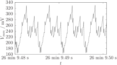
Figure 4: Compound voltage time course after establishing periodic regime (right, two periods long), and 3 seconds earlier (left).

As a parameter to analyze we take voltage at a single neuron, $v_{i}$, $i=0,\dots,24$, (several neurons have been tested) and the sum of all 25 voltages, $V_{sum}$, (1), which is the analog of the local field potential. The results are similar. Below, we present results for $V_{sum}$.

Figure 5: Chunks used for calculations. Several chunk durations have been tested, see text.

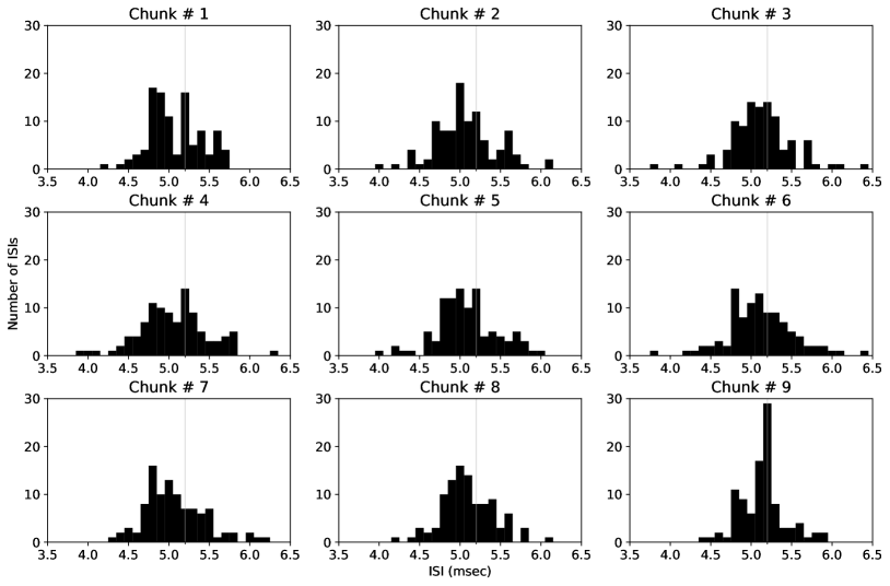
Figure 6: The ISIs histograms for the chunks # 1-9 for the neuron # 24. Here, chunk duration is 0.52 seconds. Grid lines in all figures correspond to the ISI duration 5.2 msec. Note that, in the periodic regime, the neuron # 24 fires with constant ISI duration 5.2 msec.

3.2.1 0-1 test for chaos

Here we use the binary test for chaos proposed by G. A. Gottwald and I. Melbourne, Gottwald2009 . In this test, a sequence of data

$$\mathsf{V}=\{V_{0},V_{1},\dots,V_{N-1}\}$$ (2)

can be checked for being chaotic or regular. In our case $V_{i}=V_{sum}(i)$, where $i=0,1,2,\dots N-1$, is a tick number within a chunk and $N$ is the chunk length. $\mathsf{V}$ is considered as being either regular or chaotic depending on the behavior of auxiliary two-dimensional trajectory

$$(p_{c}(n),q_{c}(n)),\quad n=0,1,\dots,N-1$$ (3)

constructed from $\mathsf{V}$ as follows:

$$p_{c}(n)=\sum\limits_{0\leq i\leq n}V_{i}\cos(i\cdot c),\quad q_{c}(n)=\sum\limits_{0\leq i\leq n}V_{i}\sin(i\cdot c)\,.$$ (4)

Here $c$ is some real number. A set of different $c$ values in the interval (0, $\pi$) are considered. If the mean square displacement of $(p_{c}(n),q_{c}(n))$ asymptotically grows linearly with $n$, than $\mathsf{V}$ is considered chaotic, otherwise if $(p_{c}(n),q_{c}(n))$ stays in a bounded domain, than $\mathsf{V}$ is regular. The asymptotic mean square displacement is defined in (Gottwald2009, , Eq. (2.1)) as follows:

$$M_{c}(n)=\lim\limits_{N\to\infty}\frac{1}{N}\sum\limits_{0\leq k<N}\left((p_{c}(k+n)-p_{c}(k))^{2}+(q_{c}(k+n)-q_{c}(k))^{2}\right),$$ (5)

which expects infinite number of points in $\mathsf{V}$. In our case, we have a finite number of points from the end of stimulation to the entrainment onto a periodic regime. Moreover, we analyze dynamics in 9 consecutive chunks before the periodic regime starts, see Fig. 5. This limits possible value of $N$ in (5) by 1743869. Thus, the modified for our case mean square displacement in each chunk is calculated as follows:

$$M_{c}(n)=\frac{1}{N_{1}}\sum\limits_{0\leq k<N_{1}}\left((p_{c}(k+n)-p_{c}(k))^{2}+(q_{c}(k+n)-q_{c}(k))^{2}\right),$$ (6)

where $n=0,1,\dots,n_{1}=1000$, and the following condition is satisfied:

$$N_{1}+n_{1}\leq N,$$

where $N$ is the chunk length.

Mean square displacement $M_{c}(n)$ oscillates with $n$, which impairs convergence. The oscillations can be subtracted from $M_{c}(n)$ as it is proposed in (Gottwald2009, , Eq. (2.3)). The resulting quantity $D_{c}(n)$ is checked for linear growth by correlation method, see (Gottwald2009, , Sec. 3.2). The correlation coefficient $K_{c}$ between sequences $\{1,2,\dots,n_{1}\}$ and $\{D_{c}(1),D_{c}(2),\dots,D_{c}(n_{1})\}$ is calculated for different values of $c$, and median in the obtained $K_{c}$ set was found. Resulting median for the first nine chunks of the trajectory is close to 1 (see Fig. 7, Table 1) qualifying those chunks as chaotic. All three values for $N$ mentioned above in Sec. 3.2 were tested with $n_{1}=1000$. The results are similar.

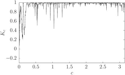
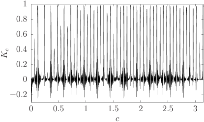
Figure 7: Behavior of correlation coefficient $K_{c}$ as a function of $c$-value. Left: chunk #9, right: chunk #10 (periodic regime). Here, chunk duration is 0.52 seconds; 1000 equidistant values of $c\in[0;\pi]$ were used for calculations.

(@,0.7cm,0.7cm)[3pt]—c—c—c—c—c—c—c—c—c—c—c——c—c—chunk number & 1 2 3 4 5 6 7 8 9 10
median of $K_{c}$ 0.992 0.994 0.993 0.994 0.993 0.994 0.993 0.994 0.992 0.026

Table 1: Result of 0-1 test for chaos in each chunk. Here, chunk duration is 0.52 seconds.

3.2.2 Permutation entropy

Complexity of trajectory $V_{sum}(t)$ in different chunks was also analyzed by calculating permutation entropy in each chunk. The permutation entropy method is proposed for estimating complexity of trajectories of a dynamical system, see Bandt2002 . In order to apply this method to a sequence of data (2), one needs to chose an embedding dimension $D>1$ and create a sequence of embedding vectors $\mathbb{V}=\{\mathbf{V}_{0},\mathbf{V}_{1},\dots,\mathbf{V}_{N-D}\}$, $\mathbf{V}_{i}\in\mathbb{R}^{D}$, $i=0,1,2,\dots N-D$, where $\mathbf{V}_{i}=(V_{i},V_{i+1},V_{i+2},\dots,V_{i+D-1})$. An additional parameter of the embedding procedure is delay, which we choose 1 here. Further step in the method is to find for each $\mathbf{V}_{i}$ a permutation $\pi_{i}$, which arranges its components in ascending order. $\pi_{i}$ is called the order pattern of $\mathbf{V}_{i}$. Having a sequence of order patterns $\Pi=\,\{\pi_{0},\pi_{1},\dots,\pi_{N-D}\}$, we calculate the probability $p_{i}$ of any of $D!$ possible patterns by dividing the number of its occurrences in $\Pi$ by the total number of elements in $\Pi$. The permutation entropy of $\mathbb{V}$ is the Shannon entropy of the probability distribution $p(\pi_{i})$:

$$S(\mathbf{\mathbb{V}})\equiv S(\Pi)=-\sum\limits_{i=0}^{M-1}p(\pi_{i})\log(p(\pi_{i})),$$

where $M$ is the number of different permutations in the $\Pi$. In this work we use a modification of this method, arithmetic entropy, which is exempt of combinatorics, see Vidybida2020 . Both methods deliver the same value for entropy provided that in any embedding vector all $D$ components are different, see (Vidybida2020, , Theorem A.1). In our case, we registered voltages with nine decimal places, therefore equalities are improbable. Additionally, in the program we developed, a check for equality between components of embedding vector was introduced, and we observed no equal components in $\mathbf{V}_{i}$. The resulting entropy values are shown in Fig. 8.

Figure 8: Permutation entropy for different embedding dimensions $D$ calculated for $V_{sum}$ in chunks shown in Fig. 5. Here, chunk duration is 0.52 seconds. The embedding delay $\tau=1$.

From these data we see that the trajectory $V_{sum}(t)$ has high complexity, roughly the same for the first 8 chunks. In the ninth chunk, complexity decreases slightly, and falls to lower values at the tenth chunk. In the periodic regime, the permutation entropy is still considerably high. This can be understood having in mind that the periodic regime itself is still quite complex, see Fig. 4 (right). For embedding dimensions considered, except of $D=3$, periodic part of the trajectory produces enough different order patterns.

3.2.3 Spectral entropy

Spectral entropy is one of nonlinear dynamics and chaos theory methods used to analyze EEG signals, Rodriguez-Bermudez2015 . Different entropy measures can be used to detect epileptic seizure on EEG. In a review Acharya2015 , it was concluded that the spectral entropy is among the best entropy measures to perform in this task. Also different entropy measures, including the spectral entropy, are used to classify emotions from EEG in a brain-computer interface, see recent review Patel2021 . Additionally, applied to local field potential measurements, correlation of time varying spectral entropies is used to detect synchrony in neural networks Kapucu2016 . Therefore, we have tested the transient with this metod.

Firstly, different chunks of the trajectory $V_{sum}(t)$ were analyzed by calculating the spectral power density (PSD) and subsequently the power spectral entropy (PSE). The algorithm used to calculate PSD is as follows. In the current work, during the course of computer simulation, the sum of voltages of all 25 neurons $V_{sum}$ (1) was sampled at discrete times with step $dt$. For one chunk, sampled $V_{sum}$ is given by $\mathsf{V}$ as in (2) with $N=5200$, where $N$ is the size of a chunk. Firstly, one needs to calculate the discrete Fourier transform of the sequence $\mathsf{V}$:

$$\mathsf{\tilde{V}}=\{\tilde{V}_{0},\tilde{V}_{1},\dots,\tilde{V}_{N-1}\}.$$ (7)

Then, from the discrete Fourier transform of $\mathsf{V}$, the PSD at the frequency $f_{k}=\frac{k}{Ndt}$, $k=1,\ldots,N/2$, can be calculated using the following expression:

$$PSD(f_{k})=\dfrac{|\tilde{V}_{k}|^{2}dt}{N}.$$ (8)

The PSD was calculated for all ten chunks. For the chunks #1 and #10, the PSD is depicted on Fig. 9. Note that on the chunk #10 (periodic activity, lower panel of Fig. 9) the frequency 1/5.2 kHz and its harmonics have the most power, while on the chunk #1 (upper panel of Fig. 9) wide peaks in the vicinity of the frequency 1/5.2 kHz and its harmonics are present.

The PSE, or Shannon spectral entropy, is an application of Shannon entropy expression to the power spectral density components Acharya2015 . To calculate the PSE, the PSD is usually normalized with the total power:

$$PSD_{norm}(f_{k})=\dfrac{PSD(f_{k})}{\sum_{l=1}^{N/2}PSD(f_{l})}.$$ (9)

Then the power spectral entropy is given by the following formula:

$$PSE=-\dfrac{1}{\log_{2}\left(N/2\right)}\sum_{k=1}^{N/2}PSD_{norm}(f_{k})\log_{2}\left(PSD_{norm}(f_{k})\right).$$ (10)

Note that here the PSE is normalized with $\log_{2}\left(N/2\right)$, which is the maximal PSE of a white noise having equal intensity at all frequencies.

The normalized PSE was calculated for chunks #1-10. The results of calculations are depicted on Fig. 10. The PSE is roughly the same for the chunks #1-9 during the relaxation to periodic activity, and sharply drops on the chunk #10 for periodic activity.

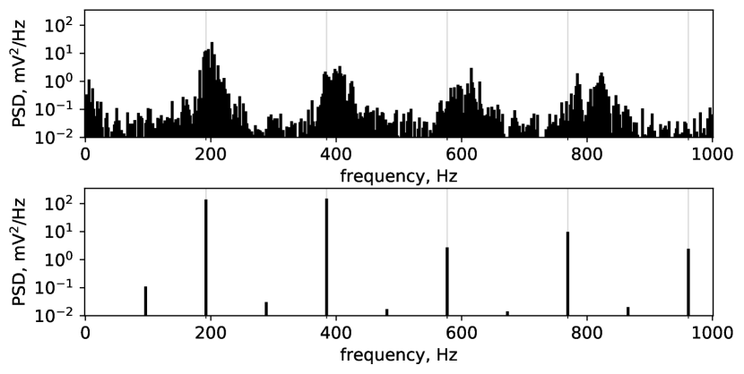
Figure 9: The power spectral density (PSD) of the sum of voltages of all 25 neurons $V_{sum}$ (1) calculated on the chunks # 1 (upper panel) and #10 (lower panel). Only frequencies up to 1 kHz are shown. Grid lines in both figures correspond to the frequency 1/5.2 kHz and its harmonics.

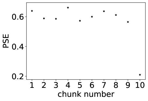
Figure 10: The normalized power spectral entropy (PSE). X-coordinate of a star indicates the chunk number.

3.2.4 Sensitivity to small perturbations

It is known that for chaotic dynamical systems small perturbations of initial state are able to produce large divergence of resulting trajectories. In our case, initial state is achieved at the end of a stimulus applied to the standard state with empty neurons and axons. Naturally, small difference between initial stimuli results in small difference in the network’s initial state. Therefore, and having in mind that a network is aimed at processing initial input into an output, we consider here small perturbations of the initial stimulus. A stimulus specificity is determined by moments of initial triggering of each neuron, see Fig. 2. Since we have a finite time step $dt=100\mu s$, the smallest possible perturbation of the stimulus can be prepared by shifting triggering moment of a single neuron by $\pm dt$. This gives 50 different stimuli characterized by the smallest possible deviation from the initial one. Each perturbed stimulus was applied and resulting dynamics was analyzed. The summary is presented in the Table 2. We see that some of the perturbed stimuli cause dynamics which ends up with periodic regime with other period than the unperturbed one. This can be treated as sensitive dependence on initial conditions/stimulus, which characterizes chaotic dynamics.

(@,0.6cm,0.7cm)[5pt]—c—c—c—c——c—c—c—c—c—c—c—c— Period, ms & Number of spikes each neuron emits per period Number of cases Relaxation time, s
activit0 (activity fades) 0 2 0.08, 0.09
9.6 2 3 60 - 436
9.7 2 2 30, 257
9.8 2 2 344
10.0 2 2 368
10.4 2 35 26 - 1569 (26 min)
41.6 8 5 36 - 722

Table 2: Result of checking stability with respect to perturbation of the initial stimulus.

4 Conclusions and discussion

In this report, in a simple deterministic neural network simulated in a PC, we have observed a remarkable dynamics in which, after a short initial stimulation, a very long chaotic transient comes to a periodic activity. This is not the first observation of this type in a simulated neuronal network, see, e.g. Zumdieck2004 ; Zillmer2009 . In our case, external intervention is given as a short initial stimulus after which dynamics runs by itself. In the previous observations external input is constantly present.

We have checked the transient observed for being chaotic by several known methods. In this connection it should be noted that standard definition of chaos is made for systems with continuous trajectories in a metric space (see a discussion of exact Devaney’s definition of chaos in Banks1992 ). In our case, trajectories are not continuous: each neuronal firing produces a discontinuity. Also, due to the numerical modeling, our trajectories are confined in a finite set of state points. Therefore, straightforward application of chaos definition made for continuous systems does not make sense in our case. The methods applied here (0-1 test for chaos, spectral and permutation entropy estimates of complexity) do not expect continuity and can be applied to discontinuous trajectories. The appealing property of chaos known as sensitive dependence on initial conditions expects a possibility to consider infinitesimally small perturbations of initial conditions, see Banks1992 . In our case, the smallest possible perturbations are finite. Some of these perturbations result in trajectories differing qualitatively from the unperturbed one, see Table 2.

The reason for a neural network to reproduces chaos can be various, see Faure2001 for discussion. Our modeling algorithm operates in whole numbers excluding possibility of rounding errors. Also, no noise is considered. It seems that the only reason for complex behavior in our network is a kind of neural computation performed due to neuronal firings and resulting in rearrangement of interspike intervals in accordance with the rules imposed by the interneuronal communication delays and LIF neuron parameters. This is a kind of self-organization in the time domain envisioned by D. M. MacKay, MacKay1962 . The computation ends when the periodic mode is reached or the activity fades. Different stimuli can cause different periodic modes in the same network. In our previous work Vidybida2011 ; Vidybida2017a made for smaller networks similar behavior has been observed, but with short transients.

In this connection a question arises: To what extent the structure of a neuronal network (“connectome”, Sporns2005 ) determines its function? From the point of view of physics the answer should be the following: completely. But it appeared quite difficult to map brain structure to function (if function is considered as a concrete dynamics evoked by a concrete stimulus) based exclusively on the connectome. The idea of a “dynome” was proposed as some additional rules governing the dynamics, Bargmann2013 ; Kopell2014 . In parallel, concepts of “functional connectome”, Biswal2010 , or “dynamic connectome”, Kringelbach2020 , were proposed. In these concepts, connections in the brain can be functionally/dynamically reconfigured depending on the cognitive task, or neuromodulator presence. As a result, complex brain dynamics are generated. The case reported here, see also Vidybida2011 ; Vidybida2017a , demonstrates that complex, stimulus dependent dynamic repertoires can also be generated without external intervention in a deterministic recurrent network with fixed connectome exclusively due to the numbers game performed in the process of neural computation.

Acknowledgments. This work was supported by the Programs of Basic Research of the Department of Physics and Astronomy of the National Academy of Sciences of Ukraine “Noise-induced dynamics and correlations in nonequilibrium systems”, № 0120U101347. AV thanks to V. Mochulska for a good literature survey during her undergraduate study in Taras Shevchenko National University of Kyiv.

References

- (1) U. R. Acharya, H. Fujita, V. K. Sudarshan, S. Bhat, and J. E. W. Koh. Application of entropies for automated diagnosis of epilepsy using eeg signals: A review. Knowledge-Based Systems, 88:85–96, 2015.
- (2) A. Babloyantz, J. M. Salazar, and C. Nicolis. Evidence of chaotic dynamics of brain activity during the sleep cycle. Physics Letters A, 111(3):152–156, 1985.
- (3) Ch. Bandt and B. Pompe. Permutation entropy: A natural complexity measure for time series. Physical Review Letters, 88(17):174102, 2002.
- (4) J. Banks, J. Brooks, G. Cairns, G. Davis, and P. Stacey. On devaney’s definition of chaos. The American Mathematical Monthly, 99(4):332–334, 1992.
- (5) C. I. Bargmann and E. Marder. From the connectome to brain function. Nature Methods, 10(6):483–490, 2013.
- (6) B. B. Biswal, M. Mennes, Xi-N. Zuo, S. Gohel, C. Kelly, S. M. Smith, C. F. Beckmann, J. S. Adelstein, Randy L. Buckner, Stan Colcombe, Anne-Marie Dogonowski, Monique Ernst, Damien Fair, Michelle Hampson, Matthew J. Hoptman, James S. Hyde, Vesa J. Kiviniemi, Rolf Kötter, Shi-Jiang Li, Ching-Po Lin, Mark J. Lowe, Clare Mackay, David J. Madden, Kristoffer H. Madsen, Daniel S. Margulies, Helen S. Mayberg, Katie McMahon, Christopher S. Monk, Stewart H. Mostofsky, Bonnie J. Nagel, James J. Pekar, Scott J. Peltier, Steven E. Petersen, Valentin Riedl, Serge A. R. B. Rombouts, Bart Rypma, Bradley L. Schlaggar, Sein Schmidt, Rachael D. Seidler, Greg J. Siegle, Christian Sorg, Gao-Jun Teng, Juha Veijola, Arno Villringer, Martin Walter, Lihong Wang, Xu-Chu Weng, Susan Whitfield-Gabrieli, Peter Williamson, Christian Windischberger, Yu-Feng Zang, Hong-Ying Zhang, F. Xavier Castellanos, and Michael P. Milham. Toward discovery science of human brain function. Proceedings of the National Academy of Sciences, 107(10):4734, 2010.
- (7) M. Breakspear. Dynamic models of large-scale brain activity. Nature Neuroscience, 20(3):340–352, 2017.
- (8) Ph. Faure and H. Korn. Is there chaos in the brain? i. concepts of nonlinear dynamics and methods of investigation. Comptes Rendus de l’Académie des Sciences - Series III - Sciences de la Vie, 324(9):773–793, 2001.
- (9) G. A. Gottwald and I. Melbourne. On the implementation of the 0–1 test for chaos. SIAM Journal on Applied Dynamical Systems, 8(1):129–145, 2009.
- (10) F. E. Kapucu, I. Välkki, J. E. Mikkonen, C. Leone, K. Lenk, J. M. A. Tanskanen, and J. A. K. Hyttinen. Spectral entropy based neuronal network synchronization analysis based on microelectrode array measurements, 2016.
- (11) N. J. Kopell, H. J. Gritton, M. A. Whittington, and M. A. Kramer. Beyond the connectome: The dynome. Neuron, 83(6):1319–1328, 2014.
- (12) H. Korn and Ph. Faure. Is there chaos in the brain? ii. experimental evidence and related models. Comptes Rendus Biologies, 326(9):787–840, 2003.
- (13) M. L. Kringelbach, J. Cruzat, J. Cabral, G. M. Knudsen, R. Carhart-Harris, P. C. Whybrow, N. K. Logothetis, and G. Deco. Closing the gap between mind and brain with the dynamic connectome. Proceedings of the National Academy of Sciences, 117(18):9677, 2020.
- (14) D. M. MacKay. Self-organization in the time domain. In M. C. Yovitz, G. T. Jacobi, and G. Goldstein, editors, Self-Organizing Systems, pages 37–48. Spartan Books, 1962.
- (15) P. Patel, R. R, and R. N. Annavarapu. Eeg-based human emotion recognition using entropy as a feature extraction measure. Brain Informatics, 8(1):20, 2021.
- (16) R. Pool. Is it healthy to be chaotic? Science, 243(4891):604–607, 1989.
-
(17)
G. Rodriguez-Bermudez and P. J. Garcia-Laencina.
Analysis of eeg signals using nonlinear dynamics and chaos: a review.
Applied mathematics
& information sciences, 9(5):2309, 2015. - (18) S. J. Schiff, K. Jerger, D. H. Duong, T. Chang, M. L. Spano, and W. L. Ditto. Controlling chaos in the brain. Nature, 6491:615–620, 1994.
- (19) A. Skarda and W. J. Freeman. How brains make chaos in order to make sense of the world. Behavioral and Brain Sciences, 10:161–195, 1987.
- (20) O. Sporns, G. Tononi, and R. Kotter. The human connectome: A structural description of the human brain. PLOS Computational Biology, 1(4):e42 EP –, 2005.
- (21) T. Tél. The joy of transient chaos. Chaos: An Interdisciplinary Journal of Nonlinear Science, 25(9):097619, 2015.
- (22) A. Vidybida and O. Shchur. Information reduction in a reverberatory neuronal network through convergence to complex oscillatory firing patterns. BioSystems, 161:24–30, 2017.
- (23) A. K. Vidybida. Testing of information condensation in a model reverberating spiking neural network. International Journal of Neural Systems, 21(3):187–198, 2011.
- (24) A. K. Vidybida. Simulating leaky integrate-and-fire neuron with integers. Mathematics and Computers in Simulation, 159:154–160, 2019.
- (25) A. K. Vidybida. Calculating permutation entropy without permutations. Complexity, 2020:7163254, 2020.
- (26) R. Zillmer, N. Brunel, and D. Hansel. Very long transients, irregular firing, and chaotic dynamics in networks of randomly connected inhibitory integrate-and-fire neurons. Physical Review E, 79(3):031909, 2009.
- (27) A. Zumdieck, M. Timme, T. Geisel, and F. Wolf. Long chaotic transients in complex networks. Physical Review Letters, 93(24):244103, 2004.