LFTC - 22 - 4/72

Pion model with the Nakanishi Integral Representations

Abstract

In the present work, we describe a model for the pion based on an analytic expression for the Bethe-Salpeter (BSA) amplitude, combined with some ingredients from Lattice QCD calculations. The running quark mass function $M(p^{2})$, used here, reproduces well the results of Lattice QCD calculations. The analytical form of the running quark mass function contains a single time-like pole, which implies in time-like poles of the dressed quark propagator. Such a form allows to build the weight functions, $G_{i}(\gamma,z)$, for the Nakanishi integral representation of each scalar function, $\chi_{i}(k,p)$, appearing in the decomposition of the Bethe-Salpeter amplitude in terms of Dirac operators, Such scalar amplitudes can also be used to obtain the pion valence light-front wave function.

Nowadays, the pion is understood as a pseudo-scalar bound state of constituents carrying the fundamental degrees of freedom of the strong interaction theory and, due to its small mass at the hadronic scale, it is considered a Goldstone boson [1]. The special nature of the pion is associated with the spontaneous breaking of chiral symmetry, where the light quarks acquires, dynamically, sizable masses departing from their small current quark masses due to weak Higgs coupling. A trace of that is found in the small pion mass (0.140 GeV), which would be zero for vanishing current quark masses when the chiral symmetry is exact. Therefore, the pion acquires a mass by the explicit breaking of this symmetry, and it is the Goldstone boson associated with the Dynamical Chiral Symmetry Breaking phenomena (DCSB), which is well established within the theory of strong interactions, namely Quantum Chromodynamics (QCD) [2]. While the current masses of the light quarks are small, the heavy ones have their large masses basically due to the Higgs coupling, breaking strongly the flavor symmetry, which was explored in a recent study of the flavor content of the light and heavy pseudoscalar mesons [3].

In the present work, we will use the results from QCD calculations in the Landau gauge on the Euclidean Lattice [4] for the dressed light quarks running masses, as proposed in [5] to model the quark propagator and the pion Bethe-Salpeter amplitude. Our aim is to explore the Nakanishi integral representation of the pion Bethe-Salpeter amplitude by computing each weight function, $G_{i}(\gamma,z)$, associated with the four scalar functions, $\chi_{i}(k,p)$, found in the decomposition of the pion Bethe-Salpeter amplitude in Dirac spinorial space.

The general form of the dressed quark propagator is given by:

$$S_{F}(k)=\imath\,Z(k^{2})\left[/k-M(k^{2})+\imath\epsilon\right]^{-1}\ ,$$ (1)

for the light quarks, namely, $u$ and $d$. The dressed quark mass function is $M(k^{2})$, which is chosen to reproduce the results obtained from Euclidean Lattice QCD (LQCD) calculations [4]. The quark wave function renormalization factor is taken here as $Z(k^{2})=1$, for simplification of the model [5], while it still captures the main physics of the QCD dynamical chiral symmetry breaking brought by the running dressed quark mass function.

The model dressed quark propagator is given by:

$$S_{F}(k)=\imath\frac{/k+[m_{0}-m^{3}(k^{2}-\lambda^{2}+\imath\epsilon)^{-1}]}{\left(k^{2}-([m_{0}-m^{3}(k^{2}-\lambda^{2}+\imath\epsilon)^{-1})^{2}]+\imath\epsilon\right)}~{},$$ (2)

in which we can identify the running quark dressed mass function:

$$M(k^{2})=m_{0}-m^{3}\left[k^{2}-\lambda^{2}+i\epsilon\right]^{-1}\,,$$ (3)

where $m_{0}=0.014\,\text{GeV},\,\,m=0.574\,\text{GeV}\,\,\text{and}\,\,\lambda\,=\,0.846\,\text{GeV}$. For convenience, we call this set as input parameters (IP) [5, 6].

They are chosen to fit the dressed light quark mass from LQCD [4] (see also [7, 8]) for space-like momenta as reproduced in the left panel of Fig. [1].

The dressed quark propagator in the present model has time-like poles, found by solving $m^{2}_{i}=M^{2}(m^{2}_{i})$, which allows to write it in a factorized form:

$$S_{F}(k)=\imath\,\,\frac{\left(k^{2}-\lambda^{2}\right)^{2}\,(/k+m_{0})-\left(k^{2}-\lambda^{2}\right)\,m^{3}}{{\prod_{i=1,3}}(k^{2}-m^{2}_{i}+\imath\epsilon)}.$$ (4)

With the set (IP), we have the following poles masses, $m_{1}=$ 0.371 GeV, $m_{2}=$ 0.644 GeV and $m_{3}=$ 0.954 GeV [5].

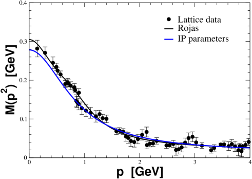
Figure 1: Top panel: dressed quark running mass for the present model in the space-like momentum region, compared with LQCD results in the Landau gauge [4], and the parametrization from Rojas et al. [7]. Bottom panel: diagrammatic representation of the Bethe-Salpeter Amplitude.

The dressed quark propagator can be written as following

$$S_{F}(k)=\imath\,\left[A(k^{2})\,/k+B(k^{2})\right]\,,$$ (5)

which by comparison with Eq.(4), one gets the explicit expressions for $A(k^{2})$ and $B(k^{2})$, as:

$$A(k^{2}) = \dfrac{\left(k^{2}-\lambda^{2}\right)^{2}}{{\prod_{i=1,3}}(k^{2}-m^{2}_{i}+\imath\epsilon)}\,,$$

$$B(k^{2}) = \dfrac{(\lambda^{2}-k^{2})m^{3}}{{\prod_{i=1,3}}(k^{2}-m^{2}_{i}+\imath\epsilon)}\,+\,m_{0}\,A(k^{2})\,.$$ (6)

We can decompose $A(k^{2})$ and $B(k^{2})$ in the form of polynomials as:

$$A(k^{2}) = \sum_{i=1}^{3}\frac{D_{i}}{k^{2}-m_{i}^{2}}$$

$$\,\,\text{and}\,\,B(k^{2}) = \-\-\-\-\sum_{i=1}^{3}\frac{m_{0}D_{i}-E_{i}}{k^{2}-m_{i}^{2}}\,,$$ (7)

where the residue are obtained from the set (IP):

$$D_{1}=1.4992,\,D_{2}=-0.5941,\,D_{3}=-0.09498,$$

$$E_{1}=0.4240,\,E_{2}=-0.3314,\,E_{3}=-0.07864\,,$$

with $D_{i}$ dimensionless and $E_{i}$ in units of GeV.

For our purpose, we can also describe the functions $A(k^{2})$ and $B(k^{2})$ in terms of a spectral representation:

$$A(k^{2}) = \int_{0}^{\infty}d\mu^{2}\frac{\rho_{A}(\mu^{2})}{k^{2}-\mu^{2}+\imath\varepsilon},\$$

$$B(k^{2}) = \int_{0}^{\infty}d\mu^{2}\frac{\rho_{B}(\mu^{2})}{k^{2}-\mu^{2}+\imath\varepsilon}\ ,$$ (8)

where the spectral densities are:

$$\rho_{A}(\mu^{2})=-\frac{1}{\pi}\,\text{Im\,}[A(\mu^{2})]\,\,\,\,\text{and}\,\,\,\,\rho_{B}(\mu^{2})=-\frac{1}{\pi}\,\text{Im\,}[B(\mu^{2})]~{}.$$

One can easily check that the model spectral functions violate the positivity constraints [1]:

$$\mathcal{P}_{a}=\rho_{A}(\mu^{2})\geq 0\,\,\,\,\text{and}\,\,\,\,\mathcal{P}_{b}=\mu\,\rho_{A}(\mu^{2})-\rho_{B}(\mu^{2})\geq 0\,,$$

which is not a problem as the quark cannot be an asymptotic state, as it should be confined within the hadron.

Remembering that we can write the functions $A(k^{2})$ and $B(k^{2})$ as a sum of polynomials, and combining with the spectral representation,

$$\int_{0}^{\infty}d\mu^{2}\frac{\rho_{A}(\mu^{2})}{k^{2}-\mu^{2}+i\epsilon}=$$

$$\sum_{i=1}^{3}\int_{0}^{\infty}d\mu^{2}\frac{D_{i}~{}\delta(\mu^{2}-m_{i}^{2})}{k^{2}-\mu^{2}+i\epsilon}$$ , (9)

we find the spectral density:

$$\rho_{A}(\mu^{2})=D_{1}\,\delta(\mu^{2}-m_{1}^{2})+D_{2}\,\delta(\mu^{2}-m_{2}^{2})+D_{3}\,\delta(\mu^{2}-m_{3}^{2}).$$

For $B(k^{2})$, the spectral decomposition is given by:

$$\int_{0}^{\infty}d\mu^{2}\frac{\rho_{B}(\mu^{2})}{k^{2}-\mu^{2}+i\epsilon}=$$

$$\sum_{i=1}^{3}\int_{0}^{\infty}d\mu^{2}\frac{E_{i}~{}\delta(\mu^{2}-m_{i}^{2})}{k^{2}-\mu^{2}+i\epsilon}.$$ (10)

We obtain, for $\rho_{B}$, the following final expression

$$\rho_{B}(\mu^{2}) = E_{1}\,\delta(\mu^{2}-m_{1}^{2})+E_{2}\,\delta(\mu^{2}-m_{2}^{2})$$

$$+ E_{3}\,\delta(\mu^{2}-m_{3}^{2})+m_{0}\,\rho_{A}(\mu^{2}).$$

In the present work, we use the Nakanishi Integral Representation (NIR), (see in  [9, 10] for more references), in order to write the Bethe-Salpeter amplitude for the pion quark-antiquark bound state. The first step is to write the pion-quark-antiquark vertex, denoted by $\Gamma_{\pi}(k,p)$, which composes the pion Bethe-Salpeter amplitude, diagrammatically represented in the right panel of Fig. 1. The most general form is given by:

$$\Gamma_{\pi}(k,p)=\gamma_{5}[\imath E_{\pi}(k,p)+/pF_{\pi}(k,p)\qquad\qquad$$

$$+k^{\mu}p_{\mu}\ /kG_{\pi}(k,p)+\sigma_{\mu\nu}k^{\mu}p^{\nu}H_{\pi}(k,p)]\,.$$ (11)

The pion Bethe-Salpeter amplitude has the form:

$$\Psi_{\pi}(k,p)=S_{F}(k+\tfrac{p}{2})\,\Gamma_{\pi}(k,p)\,S_{F}(k-\tfrac{p}{2}),$$ (12)

with the vertex function [5]

$$\Gamma_{\pi}(k,p)=\imath\,\mathcal{N}\,\gamma_{5}\,M(k)|_{m_{0}=0}$$

$$=-\imath\frac{\mathcal{N}\gamma_{5}m^{3}}{k^{2}-\lambda^{2}+\imath\epsilon} \,,$$ (13)

dominated by the dressed quark mass function in the chiral limit. $\mathcal{N}$ is a normalization factor.

After defining the structure of the pion vertex, we can write its BS amplitude, incorporating the dressed quark propagator, which also carries DCSB effects. Using the compact notation for the propagators, one has that:

$$\Psi_{\pi}(k,p) = -\left[A\left(k_{q}^{2}\right)/k_{q}+B\left(k_{q}^{2}\right)\right]\frac{\mathcal{N}\gamma_{5}m^{3}}{k^{2}-\lambda^{2}+\imath\epsilon}$$ (14)

$$\times\left[A\left(k_{\bar{q}}^{2}\right)/k_{\bar{q}}+B\left(k_{\bar{q}}^{2}\right)\right]\,,$$

here the quark and antiquark momentum are: $k_{q}=(k+p/2)$ and $k_{\bar{q}}=(k-p/2)$, respectively. This BS amplitude can be written in terms of its Dirac operator structure and scalar functions:

$$\Psi_{\pi}(k,p) = \gamma_{5}\,\chi_{1}(k,p)+\not k_{q}\gamma_{5}\,\chi_{2}(k,p)$$ (15)

$$+ \gamma_{5}k_{\bar{q}}\,\chi_{3}(k,p)+\not k_{q}\gamma_{5}k_{\bar{q}}\,\chi_{4}(k,p)\,.$$

We aim to obtain the NIR weight functions of each scalar function $\chi_{i}(k,p)$ within the present chosen analytical model for the BS amplitude. For this purpose, we introduce the useful identity given below:

$$\frac{1}{[(k+\frac{p}{2})^{2}-\mu^{\prime 2}+\imath\epsilon][k^{2}-\lambda^{2}+\imath\epsilon][(k-\frac{p}{2})^{2}-\mu^{2}+\imath\epsilon]} =$$

$$\int_{0}^{\infty}d\gamma\int_{-1}^{1}dz\frac{{F}(\gamma,z~{};\mu^{\prime},\mu)}{\left[k^{2}+z\,k\cdot P+\gamma+\imath\epsilon\right]^{3}},\ \ \$$ (16)

where

$${F}(\gamma,z~{};\mu^{\prime},\mu)=\frac{2~{}\theta(1+z-2\alpha)~{}\theta(\alpha-z)~{}\theta(1-\alpha)~{}\theta(\alpha)}{|2\lambda^{2}+M^{2}/4-\mu^{\prime^{2}}-\mu^{2}|},$$

and

$$\alpha(\gamma,z~{};\mu^{\prime},\mu)=\frac{\gamma-z(\mu^{2}-\lambda^{2}-M^{2}/4)+\lambda^{2}}{2\lambda^{2}+M^{2}/4-\mu^{2}-\mu^{\prime^{2}}}.$$

We can identify the four scalar functions of our model as:

$$\chi_{1}(k,p)=-B(k_{q}^{2})~{}\frac{m^{3}\mathcal{N}}{k^{2}-\lambda^{2}+\imath\epsilon}~{}B(k_{\overline{q}}^{2})\,,$$

$$\chi_{2}(k,p)=-A(k_{q}^{2})\frac{m^{3}\mathcal{N}}{k^{2}-\lambda^{2}+\imath\epsilon}~{}B(k_{\overline{q}}^{2})\,,$$

$$\chi_{3}(k,p)=-B(k_{q}^{2})~{}\frac{m^{3}\mathcal{N}}{k^{2}-\lambda^{2}+\imath\epsilon}~{}A(k_{\overline{q}}^{2})\,,$$

$$\chi_{4}(k,p)=-A(k_{q}^{2})\frac{m^{3}\mathcal{N}}{k^{2}-\lambda^{2}+\imath\epsilon}A(k_{\overline{q}}^{2})\,.$$ (17)

In terms of the spectral representation of the dressed quark propagator the scalar amplitudes are

$$\chi_{i}(k;p)=-\int_{0}^{\infty}d\mu^{\prime 2}\frac{\rho_{x_{i}}\left(\mu^{\prime 2}\right)}{\left[(k+p/2)^{2}-\mu^{\prime 2}+\imath\epsilon\right]}\quad$$

$$\times\frac{\mathcal{N}\,m^{3}}{\left[k^{2}-\lambda^{2}+\imath\epsilon\right]}\int_{0}^{\infty}d\mu^{2}\frac{\rho_{y_{i}}\left(\mu^{2}\right)}{\left[(k-p/2)^{2}-\mu^{2}+v\epsilon\right]},\ \ \ \$$ (18)

with the following convention $\left(x_{1},y_{1}\right)\equiv(B,B),\,\left(x_{2},y_{2}\right)\equiv(A,B),\,\left(x_{3},y_{3}\right)\equiv(B,A),$ and $\left(x_{4},y_{4}\right)\equiv(A,A)$.

Using the integral relation from Eq. ( Pion model with the Nakanishi Integral Representations), we have that:

$$\chi_{i}(k,p)=-\mathcal{N}m^{3}\int_{0}^{\infty}d\gamma\int_{-1}^{1}dz\int_{0}^{\infty}d\mu^{{}^{\prime}2}\int_{0}^{\infty}d\mu^{2}$$

$$\times\,\rho_{x_{i}}\left(\mu^{\prime 2}\right)\rho_{y_{i}}\,\left(\mu^{2}\right)\frac{{F}\left(\gamma,z;\mu^{\prime},\mu\right)}{\left[k^{2}+z\,k\cdot p-\gamma+i\epsilon\right]^{3}}.\ \ \ \$$ (19)

A close inspection of Eq.  ( Pion model with the Nakanishi Integral Representations) allows one to write the scalar amplitudes in terms of the Nakanishi integral representation,

$$\chi_{i}(k,p)=\int_{-1}^{1}dz\int_{0}^{\infty}d\gamma\frac{G_{i}\left(\gamma,z\right)}{\left[k^{2}+z\,k\cdot p-\gamma+i\epsilon\right]^{3}}\,,$$

where the weight functions are:

$$G_{i}\left(\gamma,z\right)=\sum_{j=1}^{3}\sum_{k=1}^{3}C_{i;jk}\,\,{F}\left(\gamma,z;m_{j},m_{k}\right)\,,$$ (20)

with the coefficients given by:

$$C_{1;jk} = -\mathcal{N}m^{3}\left(E_{j}+m_{0}D_{j}\right)\left(E_{k}+m_{0}D_{k}\right)\,,$$

$$C_{2;jk} = -\mathcal{N}m^{3}D_{j}\left(E_{k}+m_{0}D_{k}\right)\,,$$

$$C_{3;jk} = -\mathcal{N}m^{3}\left(E_{j}+m_{0}D_{j}\right)D_{k}\,,$$

$$C_{4;jk} = -\mathcal{N}m^{3}D_{j}D_{k}\,.$$ (21)

Taking into account the properties under the exchange of indices of the coefficients above and the explicit form of the NIR, we have the following symmetry properties for the scalar amplitudes:

$$\chi_{1}(k,p)=\chi_{1}(-k,p),\,\,\chi_{2}(k,p)=\chi_{3}(-k,p)\,,$$

$$\chi_{4}(k,p)=\chi_{4}(-k,p)\,,$$ (22)

which of course are consistent with the ones easily derived from Eq. (17) with the explicit form of these amplitudes. These symmetries properties are also associated with the even character in $z$ for

$$G_{1}(\gamma,z) = G_{1}(\gamma,-z)~{},$$ (23)

$$\quad\text{and}\quad G_{4}(\gamma,z)=G_{4}(\gamma,-z).$$

The weight functions $G_{2}$ and $G_{3}$ in Eq. (20) are neither even or odd in $z$. However, due to the symmetry property of the function $F\left(\gamma,z;m_{j},m_{k}\right)=F\left(\gamma,-z;m_{k},m_{j}\right)$ and $C_{2;jk}=C_{3,kj}$, they are related by $G_{2}(\gamma,z)=G_{3}(\gamma,-z)$. Therefore, we chose to study combinations of them, namely, $G_{3}(\gamma,z)+G_{2}(\gamma,z)$ and $G_{3}(\gamma,z)-G_{2}(\gamma,z)$, which are even and odd in $z$, respectively.

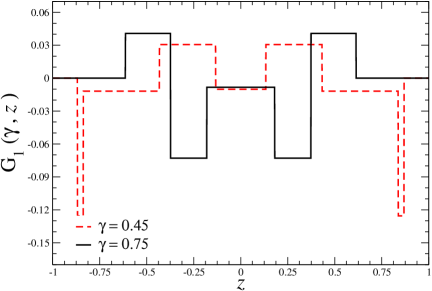
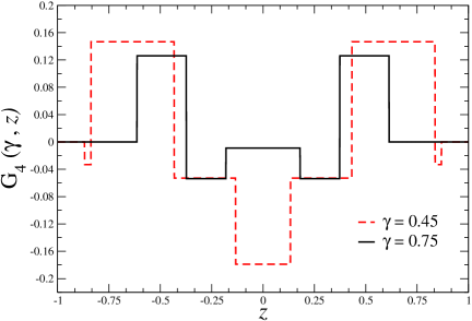
Figure 2: Left panel: $G_{1}$ weight function dependence with $z$ for $\gamma=0.45~{}\mathrm{GeV}^{2}$ (dashed line) and $0.75~{}\mathrm{GeV}^{2}$ (solid line). Right panel: $G_{4}(\gamma,z)$ as a function of $z$ with $\gamma=0.45~{}\mathrm{GeV}^{2}$ (dashed line) and $0.75~{}\mathrm{GeV}^{2}$ (solid line). The arbitrary value of $\mathcal{N}=100$ is used.

After the formal developments done so far, in what follows we present the numerical results for the four Nakanishi weight functions. For our purpose we study the dependence on $z$ of $G_{i}(\gamma,z)$ for $\gamma$ values of 0.45 and 0.75 GeV², which are within the scale of the mass poles of the dressed quark propagator and running mass function. The results are presented in figures 2 and 3. The teeth-like structure of the weight functions are due to the overlap between the theta functions present in the function $F(\gamma,z;\mu,mu^{\prime})$, which are computed over the masses of the quark propagator poles, weighted by the coefficients $C_{i;jk}$ from Eq. (21), containing the residue of the functions $A(k^{2})$ and $B(k^{2})$ in the propagator. The different signs in the residue factors $E_{i}$ and $D_{i}$, which come with $C_{i;jk}$ are reflected in the jumping of the signs of $G_{i}$ when $z$ is varied, such behavior would be softened if smooth spectral functions associated with the quark propagator are in place, however if the positivity relations are to be violated an oscillating pattern should be expected for the Nakanishi weigth functions.

We observe in figures 2 and 3 that all $G_{i}(\gamma,z=\pm 1)$ vanish due to the property of $F(\gamma,z=\pm 1;\mu,\mu^{\prime})=0$, which is essential to ensure that the pion valence light-front wave function has the correct support in the longitudinal momentum fraction, vanishing at the end-points. The $G_{i}$ are quite sensitive to the variation of $\gamma$ from 0.45 to 0.75 GeV², which reflects the relevance of the infrared physics of QCD to form the pion bound state, and responsible to give mass to the dressed quarks from the DCSB mechanism. Essentially, the observed symmetry properties of $G_{i}$ with $z$ can be traced back to the charge conjugation symmetry by the exchange of the quark and antiquark in the pion, as in our model the $u$ and $d$ quarks are identical with respect to their self-energies.

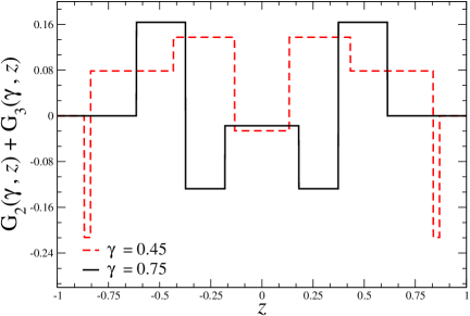
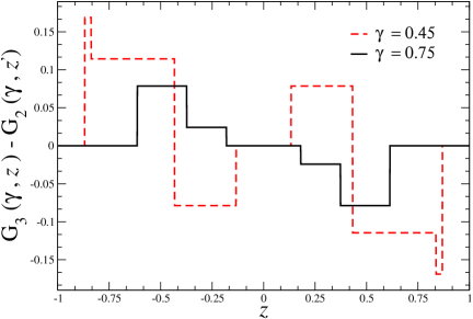
Figure 3: Left panel: $G_{2}~{}\left(\gamma,z\right)+G_{3}\left(\gamma,z\right)$ as a function of $z$ for $\gamma=0.45\ \mathrm{GeV}^{2}$ (dashed line) and $0.75\ \mathrm{GeV}^{2}$ (solid line). Right panel: $G_{3}\left(\gamma,z\right)-G_{2}\left(\gamma,z\right)$ as a function of $z$ for $\gamma=0.45~{}\mathrm{GeV}^{2}$ (dashed line) and $0.75~{}\mathrm{GeV}^{2}$ (solid line). The arbitrary value of $\mathcal{N}=100$ is used.

Finally, we should mention that the four weight functions analyzed in this contribution can be used to describe the scalar functions associated with the decomposition of the Bethe-Salpeter amplitude in the usual orthogonal basis of Dirac operators (see e.g. [9, 10]), and this will be covered in a future work, as well as the pion valence wave function [11] and momentum distributions[12], which can be written in terms of the Nakanishi weight functions provided here.

Acknowledgements:  This work was supported in part by CAPES under Grant No. 88881.309870/2018-01 (WdP), and by the Conselho Nacional de Desenvolvimento Científico e Tecnológico (CNPq), Grant No. 308486/2015-3 (TF), Process No. 307131/2020-3 (JPBCM), Grants No. 438562/2018-6 and No. 313236/2018-6 (WdP) and Fundação de Amparo à Pesquisa do Estado de São Paulo (FAPESP), Process No. 2019/02923-5 (JPBCM), and was also part of the projects, Instituto Nacional de Ciência e Tecnologia – Nuclear Physics and Applications (INCT-FNA), Brazil, Process No. 464898/2014-5, and FAPESP Temático, Brazil, Process, the thematic projects, No. 2013/26258-4 and No. 2017/05660-0.

References

[1]
C. Itzkyson and J.-B.Zuber,
”Quantum Field Theory”,
McGraw-Hill, New York,
International Series In Pure and Applied Physics, (1980), isbn 978-0-486-44568-7.
[2]
I. C. Cloët and C. D. Roberts, Explanation and Prediction of Observables using Continuum Strong QCD,
Prog. Part. Nucl. Phys. 77 (2014) 1,
https://doi.org/10.1016/j.ppnp.2014.02.001
[3]
R. Moita, J. P. B. C. de Melo, K. Tsushima and T. Frederico,
Exploring the flavor content of light and heavy-light pseudoscalars,
Phys. Rev. D 104 (2021) 096020, https://doi.org/10.1103/PhysRevD.104.096020
[4]
M. B. Parappilly, P. O. Bowman, U. M. Heller, D. B. Leinweber, A. G. Williams and J. B. Zhang,
Scaling behavior of quark propagator in full QCD, Phys. Rev. D 73 (2006) 054504,
https://doi.org/10.1103/PhysRevD.73.054504
[5]
C. S. Mello, J. P. B. C. Melo and T. Frederico, Minkowski space pion model inspired by lattice QCD running quark mass,
Phys. Lett. B766 (2017) 86,
https://doi.org/10.1016/j.physletb.2016.12.058
[6]
J. P. B. C. de Melo, R. M. Moita and T. Frederico,
Pion observables with the Minkowski Space Pion Model,
PoS LC2DOI: https://doi.org/10.22323/1.374.0037019 (2019) 037,
https://doi.org/10.22323/1.374.0037
[7]
E. Rojas, J. P. B. C. de Melo, B. El-Bennich, O. Oliveira and T. Frederico,
On the Quark-Gluon Vertex and Quark-Ghost Kernel: combining Lattice Simulations with Dyson-Schwinger equations,
JHEP 1310 (2013) 193, https://doi.org/10.1007/JHEP10(2013)193
[8]
O. Oliveira, W. de Paula, T. Frederico and J. P. B. C. de Melo, The Quark-Gluon Vertex and the QCD Infrared Dynamics,
Eur. Phys. J. C 79 (2019) 116, doi:10.1140/epjc/s10052-019-6617-7
https://doi.org/10.1140/epjc/s10052-019-6617-7
[9]
W. de Paula, T. Frederico, G. Salmè and M. Viviani,
Advances in solving the two-fermion homogeneous Bethe-Salpeter equation in Minkowski space,
Phys. Rev. D 94 (2016) 071901,
https://doi.org/10.1103/PhysRevD.94.071901
[10]
W. de Paula, T. Frederico, G. Salmè, M. Viviani and R. Pimentel,
Fermionic bound states in Minkowski-space: Light-cone singularities and structure,
Eur. Phys. J. C 77 (2017) 764,
https://doi.org/10.1140/epjc/s10052-017-5351-2
[11]
E. Ydrefors, W. de Paula, J. H. A. Nogueira, T. Frederico and G. Salmé,
,Pion electromagnetic form factor with Minkowskian dynamics,
Phys. Lett. B 820 (2021), 136494,
https://doi.org/10.1016/j.physletb.2021.136494
[12]
W. de Paula, E. Ydrefors, J. H. Alvarenga Nogueira, T. Frederico and G. Salmè,
Observing the Minkowskian dynamics of the pion on the null-plane,
Phys. Rev. D 103 (2021) 014002,
https://doi.org/10.1103/PhysRevD.103.014002