Excitation of absorbing exceptional points in the time domain

Abstract

We analyze the time-domain dynamics of resonators supporting exceptional points (EPs), at which both the eigenfrequencies and the eigenmodes associated with perfect capture of an input wave coalesce. We find that a time-domain signature of the EP is an expansion of the class of waveforms which can be perfectly captured. We show that such resonators have improved performance for storage or transduction of energy. They also can be used to convert between waveforms within this class. We analytically derive these features and demonstrate them for several examples of coupled optical resonator systems.

Optimal energy transfer via electromagnetic waves is of high importance for a variety of applications, such as transmitting information in integrated photonics and quantum processors, and energy transduction in ablation and solar cells. The limit of perfect transfer (zero scattering) in general has solutions only at discrete (possibly complex) frequencies. One form of optimal transduction of an electromagnetic wave is Coherent Perfect Absorption (CPA), the time-reversed process of lasing at threshold, in which by tuning the degree of absorption in a structure, a specific continuous wave (CW) input at real frequency will be perfectly absorbed chong2010coherent . It has recently been shown that an analogous phenomenon can be achieved in lossless systems by exciting a zero scattering state at a complex frequency with an exponentially rising input wave. In this case, the system will simply store the input until the ramp is turned off and the energy is released baranov2017coherent . Showing that it is possible to access such states raises a natural question: what are the time domain signatures of degeneracies of these states, known as exceptional points (EPs).

When a non-Hermitian system is tuned to have a degeneracy, two or more eigenvalues and eigenfunctions coalesce. EPs of resonances have been shown to lead to enhanced wave-matter interactions, improved sensing, asymmetric state transfer, and novel lasing behavior el2007theory ; makris2008beam ; wiersig2011structure ; wiersig2014chiral ; kato2013perturbation ; moiseyev2011non ; bender1998real ; guo2009observation ; ruter2010observation ; heiss2012physics ; doppler2016dynamically ; xu2016topological ; feng2017non ; zhang2018hybrid ; pick2017general ; zhang2019quantum ; zhen2015spawning ; chen2020revealing ; wang2020electromagnetically ; naghiloo2019quantum ; song2021plasmonic ; miri2019exceptional . Recently, phenomena associated with the presence of EPs of CPAs have been studied and probed in the frequency domain, focusing on real frequencies. An anomalous quartic line broadening was predicted due to the presence of the EP sweeney2019perfectly , and observed in a coupled ring resonator system, wang2021coherent . However, this earlier work considered only the CW input.

Here we show that the implication of this coalescence of eigenfunctions at a real or virtual CPA EP is that a second wave-equation solution arises, of the form $(vt-z)e^{ikz-i\omega t}$, where $v$ is the propagation speed and $k$ is the wavevector. Here $\omega,k\equiv(\omega/v)$ are real for CPA EP and complex for virtual CPA EP. More generally for an $m^{th}$ order degeneracy, solutions of the form $(vt-z)^{m-1}e^{ikz-i\omega t}$ and all lower powers exist and any superposition thereof satisfies the zero scattering boundary condition. These modes are growing temporally and decaying spatially along the propagation axis. Importantly, from time-reversal arguments one can show that the time reversal of these more general waveforms describes the emission of systems at resonance EPs heugel2010analogy ; wenner2014catching . The possibility of exciting a zero scattering state with any superposition of these waveforms hasn’t been explored prior to this work. Not only is this of fundamental interest, but it allows increased flexibility in exciting such a structure without generating reflections; we will show that this leads to improved impedance matching of finite pulses and the ability to load and potentially empty a cavity faster.

The fact that these waveforms are reflectionless can be seen from the following general argument, which applies both to CPA and the recently discussed Reflectionless Scattering Modes (RSMs). While at a CPA, with appropriate spatial excitation, there is no reflection to any of the input channels, RSMs are states which are defined by zero reflection into a chosen subset of the input channels sweeney2020theory ; dhia2018trapped , but for which the input is partially or fully transmitted into the complementary outgoing channels. For both CPA and RSMs, an eigenvalue of a suitably defined reflection matrix is zero at a particular $\omega$, and an EP of order $m$ is created by the coalescence of $m$ such frequencies and eigenvectors at $\omega_{\mathrm{EP}}$. The single remaining reflection eigenvalue vanishes as $\rho(\omega)\sim(\omega-\omega_{\mathrm{EP}})^{m}$ at the EP sweeney2019perfectly , and hence all derivatives of $\rho(\omega)$ up to order $m-1$ vanish. Specializing this to the case $m=2$, which will be our focus here, we consider inputs at $z=0$ of $e^{i\omega_{1}t}$ and $te^{i\omega_{1}t}$; we Fourier transform (FT) them, and then apply the inverse FT to their product with $\rho(\omega)$:

$$\mathcal{F}\left(e^{i\omega_{1}t}\right)=\delta\left(\omega-\omega_{1}\right),\leavevmode\nobreak\ \mathcal{F}\left(te^{i\omega_{1}t}\right)=\delta^{\prime}\left(\omega-\omega_{1}\right),$$

$$\int\delta\left(\omega-\omega_{1}\right)\rho\left(\omega\right)e^{i\omega t}d\omega=\rho\left(\omega_{1}\right)e^{i\omega_{1}t},$$ (1)

$$\int\delta^{\prime}\left(\omega-\omega_{1}\right)\rho\left(\omega\right)e^{i\omega t}d\omega=\rho^{\prime}\left(\omega_{1}\right)e^{i\omega_{1}t}+\rho\left(\omega_{1}\right)ite^{i\omega_{1}t}.$$

Thus, at a CPA or RSM EP, since $\rho\left(\omega\right)=\rho^{\prime}\left(\omega\right)=0$, there is no reflection of any linear combination of such inputs at real or complex $\omega_{\mathrm{EP}}$. This obviously applies to the inputs $t^{m-1}\exp(i\omega_{1}t)$ with $m\geq 3$ at higher-order EPs. To satisfy the wave equation, the input has to be of the form $f(vt-z)$ and we obtain the explicit solution mentioned above. In addition, it can be seen that at a generic CPA, in which only $\rho(\omega)=0$, the growing input $t\exp(i\omega t)$ is reflected but is converted to the constant-amplitude output $\exp(i\omega t).$ We will discuss such conversion processes, which generalize to higher orders, briefly below and in the SM Sec. 1.

The above argument neglects the effect of the turn on and off of the input wave. To estimate the effect of the turn on at a CPA and CPA EP, we FT the inputs of the form $\tilde{\theta}(t)e^{i\omega_{1}t}$ and $\tilde{\theta}(t)te^{i\omega_{1}t},$ where $\tilde{\theta}(t)\equiv\theta(t)\,\mathrm{or}\,(\tanh(t)+1)/2$ and multiply the results by $\rho=r$, the reflection coefficient, to get

$$\lim_{\omega\rightarrow\omega_{\mathrm{CPA}}}\mathcal{F}\left(\tilde{\theta}\left(t\right)e^{i\omega t}\right)\cdot r_{\mathrm{CPA}}\propto\frac{\omega-\omega_{\mathrm{CPA}}}{\omega-\omega_{\mathrm{CPA}}}=\mathrm{constant},$$

$$\lim_{\omega\rightarrow\omega_{\mathrm{EP}}}\mathcal{F}\left(\tilde{\theta}\left(t\right)e^{i\omega t}\right)\cdot r_{\mathrm{CPA\,EP}}\propto\frac{\left(\omega-\omega_{\mathrm{EP}}\right)^{2}}{\omega-\omega_{\mathrm{EP}}}=\left(\omega-\omega_{\mathrm{EP}}\right),$$

$$\lim_{\omega\rightarrow\omega_{\mathrm{EP}}}\mathcal{F}\left(\tilde{\theta}\left(t\right)te^{i\omega t}\right)\cdot r_{\mathrm{CPA\,EP}}\propto\frac{\left(\omega-\omega_{\mathrm{EP}}\right)^{2}}{\left(\omega-\omega_{\mathrm{EP}}\right)^{2}}=\mathrm{constant.}$$

Interestingly, we see that for input $e^{i\omega t}$ the effect of the turn on (introducing a pole) is strongly damped at CPA EP, as the response at $\omega_{\mathrm{EP}}$ is zero, whereas at a CPA it is a constant, corresponding to a slower temporal decay for the same input. In addition, while the response to $te^{i\omega t}$ at a CPA EP is also constant, the input in this second case is much larger for long excitation times, which implies smaller relative reflection. Moreover, due to the linear dependency on $t$ in $t\exp(i\omega t)$, the scattered field that originates from the incoming field at earlier times is smaller in magnitude than the current input and the scattered field before the destructive interference starts is small, which results in small relative reflection compared to $\exp(i\omega t)$.

We now demonstrate these general properties in an analytically solvable model oriented towards optics; similar excitation properties apply in AC circuits, acoustics, and quantum scattering. For simplicity we take a structure with a single input channel, terminated with a perfect mirror.

(a)

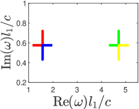
(b)

(c)

Figure 1: (a) Model of two coupled cavities terminated on the right with a perfect mirror and separated by two lossless partially reflecting mirrors of reflectivities $r_{1},r_{2}.$ At a real CPA EP $\omega_{\mathrm{EP}}$ is real and there is no scattering of the inputs associated with $\exp\left(i\omega t\right)$ and $t\exp\left(i\omega t\right).$ At a virtual CPA EP $\omega_{\mathrm{EP}}$ is complex and there is no scattering of the inputs associated with $\exp\left(i\omega_{r}t+\Gamma t\right)$ and $t\exp\left(i\omega_{r}t+\Gamma t\right),$ where $\omega_{r}\equiv\mathrm{Re}\left(\omega\right)=k_{r}v$ and $\Gamma\equiv\mathrm{Im}\left(\omega\right)=k_{i}v.$ This model can represent 3 mirrors in a uniform medium, 2 slabs, and 2 slabs with Bragg mirrors. (b) Example of a virtual CPA for the two-slab setup with $r_{2\,\mathrm{EP}}=0.574\,\,(n_{2}=4.52),r_{1\mathrm{EP}}=0.1\,(n_{1}=1.22),l_{1}=l_{2}=1$ where we varied $r_{2}.$ For this special case, additional CPA EPs occur in each free spectral range. (c) Meeting of two CPAs at a real CPA EP for the two-slab and Bragg-mirror setup as we varied $l_{2}.$ The EP is at $N_{1}=5\,\,\,N_{2}=7,\,\,\,n_{3}=1.9,$ $n_{4}=1.5,n_{1}=1.083+0.005i,\,\,\,n_{2}=2.17+0.107i,\,\,\,l_{1}=1,\,\,\,l_{2\,\mathrm{EP}}=1.5.$

A property of the response at an EP, which has been exploited for sensing applications, is that the EP leads to higher sensitivity of the eigenvalues to perturbations in the parameters of the system chen2017exceptional ; park2020symmetry ; lai2019observation ; wu2019observation . In the context of modeling this implies a higher degree of difficulty in locating EPs by pure numerical search. To avoid this, as a first step we consider the single-port three-mirror model shown in Fig. 1, which is analytically tractable and still rather general. It consists of two regions of length $l_{1},l_{2}$ and uniform refractive index $n_{1},n_{2}$ terminated by a perfect mirror. There are lossless mirrors of reflectivity $r_{1},r_{2}$ on the left surface of each region; the model can represent three specific setups (see Fig. 1a).

The total reflection amplitude coefficient for any realization of this model is give by

$$r=-\frac{r_{1}\left(e^{2ikn_{2}l_{2}}r_{2}+1\right)+e^{2ikn_{1}l_{1}}\left(r_{2}+e^{2ikn_{2}l_{2}}\right)}{1+e^{2ikn_{2}l_{2}}r_{2}+e^{2ikn_{1}l_{1}}\left(r_{2}+e^{2ikn_{2}l_{2}}\right)r_{1}}.$$ (2)

To find the EPs of this model analytically we impose the two conditions $r(\omega)=r^{\prime}(\omega)=0$ simultaneously. Defining $x=e^{2ikn_{2}l_{2}+2\pi ip},y=e^{2ikn_{1}l_{1}},$ we get

$$x =\frac{r_{2}^{2}\left(\frac{1}{\Lambda}-1\right)-\frac{1}{\Lambda}-1\pm\sqrt{\left(r_{2}^{2}\left(1-\frac{1}{\Lambda}\right)+1+\frac{1}{\Lambda}\right)^{2}-4r_{2}^{2}}}{2r_{2}},$$

$$y =r_{1}\frac{r_{2}^{2}\left(\Lambda-1\right)-\Lambda-1\text{$\mp\sqrt{\left(r_{2}^{2}\left(\Lambda-1\right)+\Lambda+1\right)^{2}-4\Lambda^{2}r_{2}^{2}}$}}{2r_{2}},$$ (3)

where $\Lambda\equiv\frac{n_{1}l_{1}}{n_{2}l_{2}}$ is the ratio of the optical lengths of the slabs. By expressing $k=\omega/c$ using $x$ and $y$ and equating, we obtain a general analytic condition for a CPA EP that holds in the weak and strong coupling regimes, (see SM Sec. V for details):

$$ye^{2\pi ip\Lambda}=x^{\Lambda}.$$ (4)

Using this method we can find quite easily continuous curves of EPs in the parameter space of the model (see Fig. S3), allowing design flexibility. Assuming $\Lambda$ is an integer, neglecting dispersion and other non-idealities, the model gives an infinite number of simultaneous EPs for the same parameter values, labeled by an integer $p.$ For $\Lambda=1,$ equal optical length, we obtain analytical solutions for the EPs

$$\frac{\omega}{c}=\frac{\ln\left(\frac{-r_{2}\left(r^{\pm}_{1}+1\right)}{2}\right)+2p\pi i}{2in_{1}l_{1}},\,\,r^{\pm}_{1}=\frac{-r_{2}^{2}+2\pm 2\sqrt{1-r_{2}^{2}}}{r_{2}^{2}}.$$

EPs for virtual CPA with $\Lambda=1$ are shown in Fig 1b. In the generic case, $\Lambda\neq 1$, the solution of Eq. (4) only gives a single EP; such an example is shown in Fig. 1c. Further examples are given in the SM Sec. V.

(a)

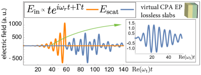
(b)

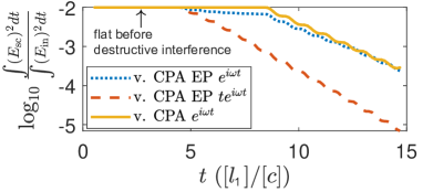
(c)

Figure 2: Scattered field at a virtual CPA EP for the inputs of (a) $e^{i\omega_{r}t+\Gamma t}$ and (b) $te^{i\omega_{r}t+\Gamma t}$ multiplied by $\left(\theta\left(t-t_{1}\right)-\theta\left(t-t_{2}\right)\right),$ where $\omega_{1}=(1.57+0.575i)/2+\pi$, same parameters as Fig. 1b, except both optical lengths are doubled. Both inputs captured almost perfectly after an initial transient; the relative scattering for $e^{i\omega_{r}t}$ is larger, see insets. (c) Relative integrated scattered energies for both inputs compared with a virtual CPA in one cavity with the same total length, Im$(\omega),$ and $r_{1}.$

We now choose an appropriate model for a virtual CPA EP and calculate the temporal response for the relevant finite-time inputs, where $\omega_{r}=\mathrm{Re}(\omega),\,\,\Gamma=\mathrm{Im}(\omega).$ To that end, we proceed similarly to Ref. karousos2008transmission , see SM Sec. VI. We present in Fig. 2 the scattered fields for the inputs $\exp(i\omega_{r}t+\Gamma t)$ (a) and $t\exp(i\omega_{r}t+\Gamma t)$ (b) multiplied by the step functions $\left(\theta\left(t-t_{1}\right)-\theta\left(t-t_{2}\right)\right),$ in a lossless two-slab system similar to that in Fig. 1 (b). As expected, after a transient, both inputs are not scattered, but the relative instantaneous scattering for the input $te^{i\omega_{1}t}$ is much smaller compared to $e^{i\omega_{1}t},$ see insets. In Fig. 2 (c) we present the relative integrated reflected energies as functions of time for both inputs in Fig. 2 (a) and (b), compared to $e^{i\omega_{1}t}$ at a virtual CPA in a single-cavity setup with the same total length, Im$(\omega),$ and $r_{1}.$ Clearly, the impedance matching is superior for both inputs at the virtual CPA EP, and the input $te^{i\omega t}$ performs significantly better. In addition, the total energy accumulated and released in the slab system is larger by two orders of magnitude for $te^{i\omega t}$ (see SM Fig. S5).

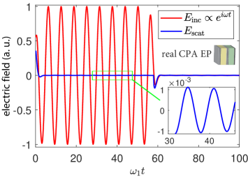
(a)

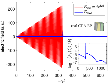
(b)

Figure 3: Scattered wave at a real CPA EP for the inputs of $e^{i\omega_{1}t}$ (a) and $te^{i\omega_{1}t}$ (b) multiplied by $\left(\tanh\left(t\right)+1-\left(\tanh\left(t-t_{1}\right)+1\right)\right)/2,$ for a high Q cavity with Bragg mirrors and EP parameters in Fig. 1. Both inputs are absorbed in steady state.

Now we calculate the temporal responses for CPA EP (real $\omega$) in a two-slab setup with loss. Here we seek efficient transduction, so we must keep track of energy which is scattered after the input is turned off. To alleviate several computational challenges, we developed a general approach to perform a numerical inverse FT of the output, see SM Sec. VI B. Since the FT of a step function decays slowly at high frequencies, we used $\tanh(t)$ as a smooth switching function. Importantly, we show there that a term in the FT of $\tilde{\theta}(t-t_{1})t\exp(i\omega t)$ is proportional to the switching-off time $t_{1}$. This implies that for $t\exp(i\omega t)$ there is negligible accumulation of unabsorbed energy at a CPA EP (due to the double zero), whereas for the conversion process, at an ordinary CPA there would be a large accumulation of unabsorbed energy in the resonator which will be emitted after turn off.

In Fig. 3 we present the temporal responses to $\exp(i\omega t)$ and $t\exp(i\omega t)$ at a real CPA EP in a high-Q two-slab setup with Bragg mirrors. In a high-Q cavity since the reflection is large and the absorption is low, the scattered field and equilibration time are larger. Evidently, at the CPA EP, the scattering from both input signals is relatively small and does decay in time while the pulse is on, as seen in the inset of Fig. 3 (b) (the moving-average of the scattered power normalized by the average incident power), implying large dissipation within the medium. For the increasing input $t\exp(i\omega t)$ it is noteworthy that negligible scattering occurs after turn off of the input, in agreement with our conclusion above. This contrasts with the response at ordinary CPA (single zero) shown in Fig. 4 in a low-Q two-slab system without Bragg mirrors. Here, $\exp(i\omega t)$ is absorbed as expected and $te^{i\omega_{1}t}$ is converted to $e^{i\omega_{1}t}$ in agreement with our CW analysis. Moreover, the scattered field in response to $e^{i\omega_{1}t}$ at the CPA is larger than at the CPA EP even though the Q-factor of the CPA EP setup is much larger, which means that the effective transient scattering at a CPA EP is much smaller (approximately 2 orders of magnitude for the times in the insets in Figs. 3 (a) and 4 (a)). Finally, after stopping the signal for the input $te^{i\omega_{1}t},$ the substantial accumulated energy is released, in agreement with our analysis above, see Fig. 4 (b).

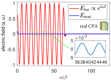
(a)

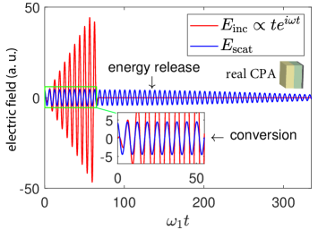
(b)

Figure 4: Scattered wave at a real CPA (not an EP) in a low-Q two-slab setup for the inputs $e^{i\omega_{1}t}$ (a) and $te^{i\omega_{1}t}$ (b) multiplied by $\left(\tanh\left(t\right)+1-\left(\tanh\left(t-50\right)+1\right)\right)/2,$ with $l_{1}=1,l_{2}=1.5,n_{1}=1.533,n_{2}=1.4+0.3i,$ $\omega_{\mathrm{CPA}}=1.27.$ It can be seen that $te^{i\omega_{1}t}$ is converted to $e^{i\omega_{1}t}$ (constant amplitude) and there is emission of the accumulated energy after the input stops.

We validate our model analysis by simulating a realistic setup of a photonic integrated circuit (PIC) that can be easily tuned to a CPA EP on the real axis, and verify its unique scattering features with full-wave simulations. The PIC consists of coupled ring-optical waveguide (CROW) resonators with a geometry that can be readily implemented using conventional PIC technology, see Fig. 5(a). The coupling parameters between the waveguides and the ring resonator $g$ and $g_{0},$ which are determined by their distances, allow us to tune the setup to a CPA EP, and in this platform they can be tuned with high accuracy using a nanopositioner stage, making it highly promising for an experimental implementation. The parameters of the setup were chosen to have the CPA EP close to the optical telecommunication wavelength $\lambda_{0}=1.56\mu\mathrm{m},$ see SM, Sec. VIII. In Fig. 5 (b) we plot the electric field distribution for a sinusoidal excitation and input power $P_{\mathrm{in}}=1$(W/m) at a CPA EP occurring at $g/g_{0}=1.08.$ As expected, there is no reflection at the right port. Finally, we plot the time domain response for both inputs in Fig. 5 (c) and (d), showcasing the same dynamics predicted in the three-mirror model.

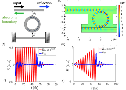
Figure 5: (a) Photonic integrated circuit (PIC) platform to realize CPA EP on real axis. (b) Electric field in the PIC at the CPA EP. (c),(d) temporal response at the EP for constant and linearly growing input pulses.

We conclude that cavities tuned to an EP provide superior performance for wave capture and impedance matching, for both energy storage (virtual case) and transduction (coherent absorption). Particularly interesting is the possibility of perfectly absorbing a linearly growing wave as well as a CW wave, which hasn’t been previously explored. The generalization of this work to higher-degeneracy EPs was mentioned above and is straightforward. While we have only shown single port realizations of absorbing structures tuned to an EP, our conclusions are valid for multiport excitation, as long as the appropriate wavefront is imposed at each port.

I Acknowledgements

We acknowledge the fruitful discussions with Tsampikos Kottos. This work was supported by a grant from the Simons Foundation. AA and AM acknowledge a grant from the Air Force Office of Scientific Research.

References

- [1] YD Chong, Li Ge, Hui Cao, and A Douglas Stone. Coherent perfect absorbers: time-reversed lasers. Physical review letters, 105(5):053901, 2010.
- [2] Denis G Baranov, Alex Krasnok, and Andrea Alu. Coherent virtual absorption based on complex zero excitation for ideal light capturing. Optica, 4(12):1457–1461, 2017.
- [3] R El-Ganainy, KG Makris, DN Christodoulides, and Ziad H Musslimani. Theory of coupled optical pt-symmetric structures. Optics letters, 32(17):2632–2634, 2007.
- [4] Konstantinos G Makris, R El-Ganainy, DN Christodoulides, and Ziad H Musslimani. Beam dynamics in pt-symmetric optical lattices. Physical Review Letters, 100(10):103904, 2008.
- [5] Jan Wiersig. Structure of whispering-gallery modes in optical microdisks perturbed by nanoparticles. Physical Review A, 84(6):063828, 2011.
- [6] Jan Wiersig. Chiral and nonorthogonal eigenstate pairs in open quantum systems with weak backscattering between counterpropagating traveling waves. Physical Review A, 89(1):012119, 2014.
- [7] Tosio Kato. Perturbation theory for linear operators, volume 132. Springer Science & Business Media, 2013.
- [8] Nimrod Moiseyev. Non-Hermitian quantum mechanics. Cambridge University Press, 2011.
- [9] Carl M Bender and Stefan Boettcher. Real spectra in non-hermitian hamiltonians having p t symmetry. Physical Review Letters, 80(24):5243, 1998.
- [10] A Guo, GJ Salamo, D Duchesne, R Morandotti, M Volatier-Ravat, V Aimez, GA Siviloglou, and DN Christodoulides. Observation of p t-symmetry breaking in complex optical potentials. Physical review letters, 103(9):093902, 2009.
- [11] Christian E Rüter, Konstantinos G Makris, Ramy El-Ganainy, Demetrios N Christodoulides, Mordechai Segev, and Detlef Kip. Observation of parity–time symmetry in optics. Nature physics, 6(3):192–195, 2010.
- [12] WD Heiss. The physics of exceptional points. Journal of Physics A: Mathematical and Theoretical, 45(44):444016, 2012.
- [13] Jörg Doppler, Alexei A Mailybaev, Julian Böhm, Ulrich Kuhl, Adrian Girschik, Florian Libisch, Thomas J Milburn, Peter Rabl, Nimrod Moiseyev, and Stefan Rotter. Dynamically encircling an exceptional point for asymmetric mode switching. Nature, 537(7618):76–79, 2016.
- [14] Haitan Xu, David Mason, Luyao Jiang, and JGE Harris. Topological energy transfer in an optomechanical system with exceptional points. Nature, 537(7618):80–83, 2016.
- [15] Liang Feng, Ramy El-Ganainy, and Li Ge. Non-hermitian photonics based on parity–time symmetry. Nature Photonics, 11(12):752–762, 2017.
- [16] Xu-Lin Zhang and Che Ting Chan. Hybrid exceptional point and its dynamical encircling in a two-state system. Physical Review A, 98(3):033810, 2018.
- [17] Adi Pick, Bo Zhen, Owen D Miller, Chia W Hsu, Felipe Hernandez, Alejandro W Rodriguez, Marin Soljačić, and Steven G Johnson. General theory of spontaneous emission near exceptional points. Optics express, 25(11):12325–12348, 2017.
- [18] Mengzhen Zhang, William Sweeney, Chia Wei Hsu, Lan Yang, AD Stone, and Liang Jiang. Quantum noise theory of exceptional point amplifying sensors. Physical review letters, 123(18):180501, 2019.
- [19] Bo Zhen, Chia Wei Hsu, Yuichi Igarashi, Ling Lu, Ido Kaminer, Adi Pick, Song-Liang Chua, John D Joannopoulos, and Marin Soljačić. Spawning rings of exceptional points out of dirac cones. Nature, 525(7569):354–358, 2015.
- [20] Hua-Zhou Chen, Tuo Liu, Hong-Yi Luan, Rong-Juan Liu, Xing-Yuan Wang, Xue-Feng Zhu, Yuan-Bo Li, Zhong-Ming Gu, Shan-Jun Liang, He Gao, et al. Revealing the missing dimension at an exceptional point. Nature Physics, 16(5):571–578, 2020.
- [21] Changqing Wang, Xuefeng Jiang, Guangming Zhao, Mengzhen Zhang, Chia Wei Hsu, Bo Peng, A Douglas Stone, Liang Jiang, and Lan Yang. Electromagnetically induced transparency at a chiral exceptional point. Nature Physics, 16(3):334–340, 2020.
- [22] M Naghiloo, M Abbasi, Yogesh N Joglekar, and KW Murch. Quantum state tomography across the exceptional point in a single dissipative qubit. Nature Physics, 15(12):1232–1236, 2019.
- [23] Qinghua Song, Mutasem Odeh, Jesús Zúñiga-Pérez, Boubacar Kanté, and Patrice Genevet. Plasmonic topological metasurface by encircling an exceptional point. Science, 373(6559):1133–1137, 2021.
- [24] Mohammad-Ali Miri and Andrea Alu. Exceptional points in optics and photonics. Science, 363(6422):eaar7709, 2019.
- [25] William R Sweeney, Chia Wei Hsu, Stefan Rotter, and A Douglas Stone. Perfectly absorbing exceptional points and chiral absorbers. Physical review letters, 122(9):093901, 2019.
- [26] Changqing Wang, William R Sweeney, A Douglas Stone, and Lan Yang. Coherent perfect absorption at an exceptional point. Science, 373(6560):1261–1265, 2021.
- [27] Simon Heugel, Alessandro S Villar, Markus Sondermann, Ulf Peschel, and Gerd Leuchs. On the analogy between a single atom and an optical resonator. Laser Physics, 20(1):100–106, 2010.
- [28] J Wenner, Yi Yin, Yu Chen, R Barends, B Chiaro, E Jeffrey, J Kelly, A Megrant, JY Mutus, C Neill, et al. Catching time-reversed microwave coherent state photons with 99.4% absorption efficiency. Physical Review Letters, 112(21):210501, 2014.
- [29] William R Sweeney, Chia Wei Hsu, and A Douglas Stone. Theory of reflectionless scattering modes. Physical Review A, 102(6):063511, 2020.
- [30] Anne-Sophie Bonnet-Ben Dhia, Lucas Chesnel, and Vincent Pagneux. Trapped modes and reflectionless modes as eigenfunctions of the same spectral problem. Proceedings of the Royal Society A: Mathematical, Physical and Engineering Sciences, 474(2213):20180050, 2018.
- [31] Weijian Chen, Şahin Kaya Özdemir, Guangming Zhao, Jan Wiersig, and Lan Yang. Exceptional points enhance sensing in an optical microcavity. Nature, 548(7666):192–196, 2017.
- [32] Jun-Hee Park, Abdoulaye Ndao, Wei Cai, Liyi Hsu, Ashok Kodigala, Thomas Lepetit, Yu-Hwa Lo, and Boubacar Kanté. Symmetry-breaking-induced plasmonic exceptional points and nanoscale sensing. Nature Physics, 16(4):462–468, 2020.
- [33] Yu-Hung Lai, Yu-Kun Lu, Myoung-Gyun Suh, Zhiquan Yuan, and Kerry Vahala. Observation of the exceptional-point-enhanced sagnac effect. Nature, 576(7785):65–69, 2019.
- [34] Yang Wu, Wenquan Liu, Jianpei Geng, Xingrui Song, Xiangyu Ye, Chang-Kui Duan, Xing Rong, and Jiangfeng Du. Observation of parity-time symmetry breaking in a single-spin system. Science, 364(6443):878–880, 2019.
- [35] Anastasios Karousos, George Koutitas, and Costas Tzaras. Transmission and reflection coefficients in time-domain for a dielectric slab for uwb signals. In VTC Spring 2008-IEEE Vehicular Technology Conference, pages 455–458. IEEE, 2008.