Efficient Massive Machine Type Communication (mMTC) via AMP

Abstract

We propose efficient and low complexity multiuser detection (MUD) algorithms for Gaussian multiple access channel (G-MAC) for short-packet transmission in massive machine type communications. We formulate the problem of MUD for the G-MAC as a compressive sensing problem with virtual sparsity induced by one-hot vector transmission of devices in code domain. Our proposed MUD algorithms rely on block and non-block approximate message passing (AMP) for soft decoding of the transmitted packets. Taking into account the induced sparsity leads to a known prior distribution on the transmit vector; hence, the optimal minimum mean squared error (MMSE) denoiser can be employed. We consider both separable and non-separable MMSE denoisers for AMP soft decoding. The effectiveness of the proposed MUD algorithms for a large number of devices is supported by simulation results. For packets of $8$ information bits, while the state of the art AMP with soft-threshold denoising achieves $5/100$ of the converse bound at $E_{b}/N_{0}=4$ dB, the proposed algorithms reach $4/9$ and $1/2$ of the converse bound.

I Introduction

Massive uplink connectivity is one of the key factors in the realization of the Internet-of-Things (IoT). In many IoT applications, massive machine-type communications (mMTC) services are required, where a large number of devices transmit very short packets to a base station (BS). Typically, these short packets are transmitted whenever a measured value changes [1, 2].

Recently, bounds on the exact block error probability of Gaussian random codes in additive white Gaussian noise (AWGN) for massive uplink multiple access (MA) at finite message length have been derived [3]. The author in [3] has shown that a promising solution to support massive uplink connectivity for short packet transmission is the Gaussian multiple access channel (G-MAC). The challenging task in the realization of G-MAC is the design of efficient and low complexity multiuser detection (MUD) algorithms at the base station (BS) to achieve the desirable spectral efficiency and reliability for short-packet transmission [4].

In this paper, we propose two efficient and low-complexity MUD algorithms for G-MAC for short-packet mMTC. We first formulate the MUD detection problem as an under-determined compressive sensing problem. Then, we employ approximate message passing (AMP) for soft decoding of the short packets transmitted by the IoT devices in the network. The flexibility in the AMP algorithm design is attributed to the denoiser ${\bm{\eta}}_{t}(\cdot)$. The denoisers in the AMP variants are typically designed to reduce the estimation error at each iteration [5].

For most problems, the prior distribution of the vector to be recovered is generally assumed to be unknown. In this case, the denoiser is designed under the minimax framework to optimize the AMP algorithm performance for the worst-case or least-favorable distribution, leading to a soft-thresholding denoiser. However, in the problem at hand, we have the exact and asymptotic empirical prior distribution of the sparse vector to be recovered. Hence, the optimal MMSE denoiser can be employed in AMP. By taking into account the exact and asymptotic prior distribution of the transmit vector, we employ separable and non-separable MMSE denoisers for Bayesian AMP. The decoupling effect results in low-complexity MMSE denoising in each AMP iteration [6, 7].

The main contributions of the paper are:

• We introduce two MUD algorithms called (i) the relaxed block sparsity AMP (RBS-AMP), and (ii) block sparsity AMP (BS-AMP) MUD algorithms for G-MAC suitable for short packet transmission in mMTC. We show that our BAMP MUD algorithm results in a new achievability bound that is closer to the converse bound in [3].

• The multiuser efficiency (MUE) of the proposed MUD algorithms is derived, and shown to be close to one.

Notation: The symbols $(\cdot)^{T}$, ${\rm Tr}(\cdot)$, $\|\cdot\|_{0}$, and $\|\cdot\|$ show the transpose operator, trace of a matrix, $0$-norm, and Euclidean norm of a vector, respectively. $\mathbb{E}\{\cdot\}$ is the statistical expectation, and $\hat{\bf{x}}$ is an estimate of vector $\bf x$. $\delta(\cdot)$ is the Dirac delta function.

II System Model

We consider a single-hop Internet of Things (IoT) network, where $D$ IoT devices simultaneously communicate with a single BS. Each IoT device transmits $K$ bits of information by using Gaussian random coding with codewords of length $M=nD$. The aggregate rate of the multiuser coded system is $DK/M$. For short packet transmission, the received vector at the BS in vector form is

$${\bf y}={\bf C}{\bf x}+{\bf w},$$ (1)

where ${\bf C}\in\mathbb{R}^{M\times N}$ has independent and identically distributed (i.i.d.) entries, $C_{ij}\sim\mathcal{N}(0,1/M)$, $N\triangleq 2^{K}D$, and ${\bf x}$ is a block sparse vector of length $N\times 1$ as

$${\bf{x}}=\big{[}{\bf{x}}_{1}^{T}\ {\bf{x}}_{2}^{T}\dots\ {\bf{x}}_{D}^{T}\big{]}^{T},$$ (2)

where ${\bf{x}}_{q}$ is a $2^{K}\times 1$ vector as $||{\bf{x}}_{q}||_{0}=1,q=1,2,\dots,D$. The $M\times 1$ vector ${\bf w}$ in (1) is the additive white Gaussian noise (AWGN) vector with covariance matrix $\sigma_{\rm w}^{2}\bf{I}$. Here, we assume that $\beta\triangleq\lim_{D\to\infty}M/N=n/(2^{K})\in>0$.

We consider that the $D$ IoT devices in the network transmit with equal power $P_{\rm{I}}$. In this case, the prior distribution for the transmit vector ${\bf x}_{q}\triangleq[x_{q,1},x_{q,2},\dots,x_{q,2^{K}}]^{\rm T}$, $q=1,2,\dots,D$, in (2) is given by

$$f_{\bf X}({\bf x}_{q};P_{\rm{I}},K)=\sum_{k=1}^{2^{K}}\frac{1}{2^{K}}\delta({\bf x}_{q}-\sqrt{P_{\rm{I}}}{\bf e}_{k}),$$ (3)

where ${\bf e}_{1},{\bf e}_{2},\cdots,{\bf e}_{2^{K}}$ are orthonormal basis in right-handed Cartesian coordinate system, i.e., ${\bf e}_{k}\triangleq[e_{1}\ e_{2}\ \cdots\ e_{2^{K}}]^{T}=[0\ 0\ \cdots\ 0\ 1\ 0\ \cdots\ 0]^{T}$ in which the $k$th element is one and the remaining elements are zero, and $\delta({\bf x}_{q})=\prod_{k=1}^{2^{K}}\delta(x_{q,k})$. Our goal is to design a MUD algorithm at the BS to detect the $K$ information bits transmitted by each IoT device. As ${\bf x}$ is a block-sparse vector, we have a sparse signal reconstruction problem. In this paper, we adopts low-complexity Bayesian AMP algorithm for signal recovery.

III Review of AMP with Different Denoisers

In this section, we first briefly review AMP algorithm with separable and non-seperable denoisers. Then, in Theorem 2, we show that the per-iteration mean-squared error of the reconstructed vector through AMP with non-seperable denoiser, can be predicted using a state evolution (SE). Theorem 2 will be later used for the derivation of the MUE of the proposed BS-MUD algorithm.

III-A AMP Algorithm with Separable Denoiser

For noisy linear measurements of the form

$${\bf s}={\bf A}{\bf u}+{\bf w},$$ (4)

where ${\bf A}\in\mathbb{R}^{M\times N}$, ${\bf s}\in\mathbb{R}^{M\times 1}$, ${\bf u}\in\mathbb{R}^{N\times 1}$, and ${\bf w}\in\mathbb{R}^{M\times 1}$. AMP algorithm with denoiser ${\bm{\eta}}_{t}$: $\mathbb{R}^{N}\rightarrow\mathbb{R}^{N}$ at the $(t+1)$th iteration estimates vector $\bf{u}$ as follows [8]

$$\hat{\bf u}^{t+1}={\bm{\eta}}_{t}({\bf v}^{t})={\bm{\eta}}_{t}(\hat{\bf{u}}^{t}+{\bf A}^{T}{\bf r}^{t}),$$ (5)

where

$${\bf r}^{t}={\bf s}-{\bf A}\hat{\bf{u}}^{t}+\frac{N}{M}{\bf r}^{t-1}{\rm div}\big{(}{\bm{\eta}}_{t-1}({\bf v}^{t-1})\big{)},$$ (6)

$${\bf v}^{t}=\hat{\bf{u}}^{t}+{\bf A}^{T}{\bf r}^{t},$$ (7)

and ${\rm div}\big{(}{\bm{\eta}}_{t}({\bf g})\big{)}\triangleq\frac{1}{N}{\rm Tr}\Big{(}\frac{\partial{\bm{\eta}}_{t}({\bf g})}{\partial{\bf g}}\Big{)}$ with ${\bf{g}}\triangleq[g_{1}\ g_{2}\dots g_{N}]^{T}$, $\hat{\bf u}^{0}=\bf{0}$, and ${\bf r}^{0}=\bf{s}$. For identical separable Lipschitz continuous (LC) denoiser, ${\bm{\eta}}_{t}({\bf g})=\big{[}{\eta}_{t}({g_{1}})\ {\eta}_{t}({g_{2}})\ \dots\ {\eta}_{t}({g_{N}})\big{]}^{T}$ and ${\rm div}\big{(}{\bm{\eta}}_{t}({\bf g})\big{)}=\frac{1}{N}\sum_{j=1}^{N}{\partial{\eta}_{t}(g_{j})}/{\partial g_{j}}.$ Similarly, for non-separable LC denoisers, we have [8]

$${\bm{\eta}}_{t}({\bf g})=\big{[}{\bm{\eta}}_{t,1}({{\bf g}_{1}})\ {\bm{\eta}}_{t,2}({{\bf g}_{2}})\ \dots\ {\bm{\eta}}_{t,L}({{\bf g}_{L}})\big{]}^{T},$$ (8)

and

$${\rm div}\big{(}{\bm{\eta}}_{t}({\bf g})\big{)}=\frac{1}{N}\sum_{m=1}^{L}{\rm Tr}\Big{(}\frac{\partial{\bm{\eta}}_{t,m}({\bf g}_{m})}{\partial{\bf g}_{m}}\Big{)},$$ (9)

where ${{\bf g}_{1}},{{\bf g}_{2}},\cdots,{{\bf g}_{L}}$ denote $L$ non-overlapping partitions of ${\bf g}$. The initial work on AMP focused on the case where $\bm{\eta}_{t}(\cdot)$ is a separable elementwise function with identical components [9], while the later work allowed non-separable blockwise denoiser [8].

For large, i.i.d., sub-Gaussian random matrices $\bf A$ in (4), $\lim_{M,N\to\infty}M/N\triangleq\beta>0$, and identical separable/non-separable LC denoiser, AMP displays decoupling behavior, meaning that ${\bf v}^{t}$ in (7) behaves like an AWGN corrupted version of the true signal $\bf{u}$ in (4) as [10]

$${\bf v}^{t}={\bf{u}}+{\cal{N}}(0,\sigma_{t}^{2}{\bf I}),$$ (10)

where an estimate of $\sigma_{t}^{2}$ can be obtained as $\hat{\sigma}_{t}^{2}=\frac{1}{M}\|{\bf{r}}^{t}\|$. The larger $M$, the lower the estimation error.

III-B SE of AMP with Separable Denoiser

For large, i.i.d., sub-Gaussian random matrices $\bf A$, the performance of AMP can be exactly predicted by a scalar SE, which also provides testable conditions for optimality. For identical separable LC denoiser $\eta_{t}(\cdot)$, when the elements of ${\bf{u}}=[u_{1},u_{2},\dots,u_{N}]$ empirically converges to some random variable $U$ with probability density function (PDF) $f_{U}$, the SE i.e., the sequence of $\{\sigma_{t}^{2}\}_{t\geq 0}$ in (10) is expressed as

$$\sigma^{2}_{t+1}=\sigma_{\rm w}^{2}+\frac{1}{\beta}\mathbb{E}\big{\{}(\eta_{t}(U+\sigma_{t}Z)-U)^{2}\big{\}},$$ (11)

where $\beta=M/N$ and

$$\sigma^{2}_{0}=\sigma_{\rm w}^{2}+\frac{1}{\beta}\mathbb{E}\big{\{}U^{2}\big{\}},$$ (12)

where $Z\sim{\cal N}(0,1)$ and is independent from $U$. The term $(\sigma^{2}_{t+1}-\sigma_{\rm w}^{2})\beta$ in (11) can be estimated by the sample mean estimate of the denoiser error as it is expressed in Theorem 1.

Theorem 1.

Let ${\bf{A}}\in\mathbb{R}^{M\times N}$ be a matrix with i.i.d. entries $A_{ij}\sim\mathcal{N}(0,1/M)$, and assume $M/N\rightarrow\beta>0$. Consider a random signal ${\bf u}\in\mathbb{R}^{N}$, whose empirical distributions converge weakly to a PDF $f_{U}$ on $\mathbb{R}$ with bounded moment of order $(2k-2)$ as $N\rightarrow\infty$ for some $k\geq 2$. Then, for any pseudo-Lipschitz function $\psi(\cdot,\cdot):\mathbb{R}^{2}\rightarrow\mathbb{R}$ of order $k$ and all $t\geq 0$, we almost surely have (Proof in [11])

$$\mathop{\lim}\limits_{N\to\infty}\frac{1}{N}\sum_{i=1}^{N}\psi(\hat{u}_{i}^{t+1},u_{i})=\mathbb{E}\big{\{}\psi(\eta_{t}(U+\sigma_{t}Z),U)\big{\}},$$ (13)

where $\hat{\bf u}^{t+1}\triangleq[\hat{u}_{1}^{t+1}\ \hat{u}_{2}^{t+1}\ \dots\ \hat{u}_{N}^{t+1}]^{T}$ is obtained by using AMP in (5)-(7), $U\sim f_{U}$, $Z\sim{\cal N}({{0}},\sigma_{t}^{2})$ is independent of $U$, and $\sigma_{t}$ follows the SE in (11) and (12). For $\psi(x,y)=(x-y)^{2}$, we have

$$\mathop{\lim}\limits_{N\to\infty}\frac{1}{N}\big{\|}\hat{\bf{u}}^{t+1}-{\bf{u}}\big{\|}_{2}^{2} =\mathbb{E}\big{\{}(\eta_{t}(U+\sigma_{t}Z)-U)^{2}\big{\}}$$ (14)

$$=(\sigma^{2}_{t+1}-\sigma_{\rm w}^{2})\beta.$$

III-C AMP with Non-separable Denoiser

Let us consider a block structure for the vector ${\bf{u}}$ in (4) as ${\bf{u}}=[{\bf{u}}_{1}^{\rm{T}},{\bf{u}}_{2}^{\rm{T}},\cdots,{\bf{u}}_{L}^{\rm{T}}]$, where ${\bf{u}}_{i}$ and ${\bf{u}}_{j}$, $i\neq j$ are independent random vectors. We consider the following cases: 1) the joint PDF of ${\bf{u}}_{i}\triangleq[u_{i,1},u_{i,2},\dots,u_{i,\ell}]^{\rm T}$ is ${\bf{U}}=[U_{1}\ U_{2}\ \dots\ U_{\ell}]^{T}\sim f_{\bf{U}}$, and 2) the empirical joint PDF of ${\bf{u}}_{i}$ converges weakly to $f_{\bf U}$, where $\ell=N/L$. AMP with identical non-separable LC denoiser in (8) with $\tilde{\bm{\eta}}_{t}(\cdot):\mathbb{R}^{\ell}\rightarrow\mathbb{R}^{\ell}$ $({\bm{\eta}}_{t,m}(\cdot)=\tilde{\bm{\eta}}_{t}(\cdot),m=1,2,\dots,L)$, reconstructs the vector ${\bf{u}}$ from the observation model in (4) through the relations in (5)-(7). Also, the decoupling behavior occurs for the $m$th block as

$${\bf v}_{m}^{t}={\bf{u}}_{m}+{\bf z}_{m}^{t},\,\,\,\,\,\,\ m=1,2,\dots,L,$$ (15)

where

$${\bf z}_{m}^{t}\sim N\big{(}{{0}},\rho_{t}^{2}{\bf{I}}\big{)}.$$ (16)

The SE i.e., the sequence of $\{\rho_{t}^{2}\}_{t\geq 0}$ in (16) is given by

$$\rho^{2}_{t+1}=\sigma_{\rm w}^{2}+\frac{1}{\ell\beta}\mathbb{E}\Big{\{}\big{\|}\tilde{\bm{\eta}}_{t}({\bf{U}}+\rho_{t}{\bf{Z}})-{\bf U}\big{\|}^{2}\Big{\}},$$ (17)

$$\rho^{2}_{0}=\sigma_{\rm w}^{2}+\frac{1}{\ell\beta}\mathbb{E}\big{\{}{\|}{\bf U}{\|}^{2}\big{\}},$$ (18)

where ${\bf Z}=[Z_{1}\ Z_{2}\ \dots\ Z_{\ell}]^{\rm T}\sim N({{0}},{\bf{I}})$ is independent of ${\bf U}=[U_{1}\ U_{2}\ \dots\ U_{\ell}]^{\rm T}\sim P_{\bf{U}}$. A modified version of Theorem 1 for identical non-separable LC denoiser is given as follows:

Theorem 2.

Let ${\bf{A}}\in\mathbb{R}^{M\times N}$ be a matrix with i.i.d. entries $A_{ij}\sim\mathcal{N}(0,1/M)$, and assume $M/N\rightarrow\beta>0$. Consider a block sparse signal ${\bf{u}}=\big{[}{\bf{u}}_{1}^{T}\ {\bf{u}}_{2}^{T}\dots\ {\bf{u}}_{L}^{T}\big{]}^{T}$, where the joint distribution of each block of length $\ell$ is $f_{\bf U}$ (or empirical joint PDF converges weakly to $f_{\bf U}$) on $\mathbb{R}^{\ell}$. Then, we have

$$\mathop{\lim}\limits_{L\to\infty}\frac{1}{L}\sum_{u=1}^{L}\big{\|}\hat{\bf u}_{u}^{t+1}-{\bf u}_{u}\big{\|}^{2}=\mathbb{E}\Big{\{}\big{\|}\tilde{\bm{\eta}}_{t}({\bf{U}}+\rho_{t}{\bf{Z}})-{\bf U}\big{\|}^{2}\Big{\}},$$ (19)

where $\hat{\bf{u}}=\big{[}\hat{\bf{u}}_{1}^{T}\ \hat{\bf{u}}_{2}^{T}\dots\ \hat{\bf{u}}_{L}^{T}\big{]}^{T}$ is obtained by using (5)-(7), ${\bf U}\sim f_{\bf U}$, ${\bf Z}\sim N({{0}},{\bf{I}})$ is independent of ${\bf U}$, and $\rho_{t}$ follows the SE in (17) and (18).

Proof.

Proof in Appendix A. ∎

IV AMP-based MUD for Short-packet Communications

In this section, we propose RBS-AMP and BS-AMP MUD algorithms for G-MAC. The former AMP-based MUD algorithm employs separable MMSE denoiser and offers lower complexity, and the latter algorithm uses block non-seperable MMSE denoiser and achieve higher decoding performance.

IV-A RBS-AMP MUD

The RBS-AMP MUD algorithm neglects the block-sparsity of $\bf{x}$ in (1) and consider the asymptotic empirical PDF. This block sparsity relaxation results in a low complexity MUD algorithm since the prior PDF in (3) is replaced with the simple asymptotic empirical PDF. The empirical distribution of the block sparse vector ${\bf{x}}=[x_{1},x_{2},\cdots,x_{N}]^{T}$ in (2) as $N\rightarrow\infty$, converges weakly to the scaled Bernoulli distribution with the PDF $f_{X}(x;P_{\rm{I}};K)$ as

$$f_{X}(x;P_{\rm{I}};K)=\frac{1}{2^{K}}\delta\big{(}x-\sqrt{P_{\rm{I}}}\big{)}+\Big{(}1-\frac{1}{2^{K}}\Big{)}\delta(x).$$ (20)

$$\mathop{\lim}\limits_{N\to\infty}\frac{1}{N}\big{\|}\hat{\bf{x}}^{t+1}-{\bf{x}}\big{\|}_{2}^{2} =\mathbb{E}\big{\{}(\eta_{t}(X+\sigma_{t}Z)-X)^{2}\big{\}}=\frac{1}{2^{K}\sqrt{2\pi\sigma_{t}^{2}}}\int_{-\infty}^{\infty}\Bigg{(}\frac{pT_{i}^{t}}{pT_{i}^{t}+1-p}-\sqrt{P_{\rm{I}}}\Bigg{)}^{2}\exp\Big{\{}-\frac{(v_{i}^{t}-\sqrt{P_{\rm{I}}})^{2}}{2\sigma_{t}^{2}}\Big{\}}{\rm d}v_{i}^{t}$$

$$+\Big{(}1-\frac{1}{2^{K}}\Big{)}\frac{1}{\sqrt{2\pi\sigma_{t}^{2}}}\int_{-\infty}^{\infty}\Bigg{(}\frac{pT_{i}^{t}}{pT_{i}^{t}+1-p}\Bigg{)}^{2}\exp\Big{\{}-\frac{(v_{i}^{t})^{2}}{2\sigma_{t}^{2}}\Big{\}}{\rm d}v_{i}^{t}=(\sigma^{2}_{t+1}-\sigma_{w}^{2})\beta$$ (26)

.  

Let us consider $\hat{\bf{x}}=[\hat{x}_{1}^{t+1},\hat{x}_{2}^{t+1},\cdots,\hat{x}_{N}^{t+1}]^{T}$, the reconstructed vector by the AMP algorithm summarized in (5)-(7) at the $(t+1)$th iteration for the observation model in (1), i.e., ${\bf s}={\bf y}$, ${\bf u}={\bf x}$, and ${\bf A}={\bf C}$. For the identical separable MMSE denoiser $\eta(\cdot)=\mathbb{E}\{\cdot|v_{i}^{t}\}$ with prior distribution $U=X\sim f_{X}(x;P_{\rm{I}};K)$ in (20), by taking into account the decoupling behavior in (10), the $i$th element of the soft decoded vector at the $(t+1)$th iteration is given by

$$\hat{x}_{i}^{t+1} =\eta({{v_{i}^{t}}})=\mathbb{E}\big{\{}X_{i}|X_{i}+\sigma_{t}Z=v_{i}^{t}\big{\}}$$ (23)

$$=\frac{pT_{i}^{t}}{pT_{i}^{t}+1-p},$$

where $Z\sim{\cal N}(0,1)$,

$$T_{i}^{t}\triangleq{\exp\Big{\{}\frac{-P_{\rm{I}}+2v_{i}^{t}{\sqrt{P_{\rm{I}}}}}{2\sigma_{t}^{2}}\Big{\}}},$$ (24)

and $p=1/{2^{K}}$. Proof of the general case for the prior PDF in (3) is given in Appendix B. Moreover, the divergence term at the $(t+1)$th iteration of the RBS-AMP in (6) is obtained as

$${\rm div}\big{(}{\bm{\eta}}_{t}({\bf v}^{t})\big{)} =\frac{1}{N}\sum_{i=1}^{N}\frac{\partial}{\partial v_{i}^{t}}\eta_{t}({{v_{i}^{t}}})$$ (25)

$$=\frac{1}{N}\sum_{i=1}^{N}\frac{\partial}{\partial v_{i}^{t}}\mathbb{E}\big{\{}X_{i}|X_{i}+\sigma_{t}Z=v_{i}^{t}\big{\}}$$

$$=\frac{p(1-p)\sqrt{P_{\rm{I}}}}{\sigma_{t}^{2}N}\sum_{i=1}^{N}\frac{T_{i}^{t}}{(pT_{i}^{t}+1-p)^{2}}.$$

In practice, the SE, i.e., $\{\sigma_{t}^{2}\}_{t\geq 0}$ is tracked by the sample mean estimate $\hat{\sigma}_{t}^{2}\approx\frac{1}{M}\|{\bf{r}}^{t}\|$, where ${\bf{r}}^{t}$ is given in (6) for ${\bf{A}}={\bf{C}}$ and $\hat{\bf{u}}=\hat{\bf{x}}$. The SE can also be theoretically obtained by using Theorem 1. In this case, from (14) and (20), we obtain (26) at the top of the next page.

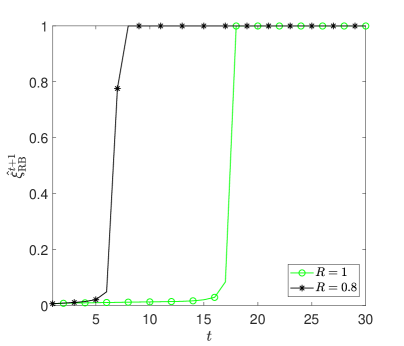
Figure 1: State evolution of the RBS-AMP with separable MMSE denoiser for $K=8$ and $U=1024$ at $5$ dB SNR.

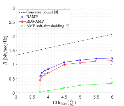
Figure 2: Spectral efficiency versus $10\log_{10}({E_{\rm b}}/{N_{0}})$ for average block error rate $P_{\rm{e}}=10^{-3}$, $K=8$, and $D=512$.

MUE of the RBS-AMP MUD algorithm: The degradation in bit error rate due to the presence of MA interference in AWGN channel can be measured by the multiuser asymptotic efficiency, which is defined as

$$\xi=\frac{\sigma_{\rm w}^{2}}{\sigma_{\rm w}^{2}+I},$$ (27)

where $\sigma_{\rm w}^{2}$ is the variance of noise, and $I$ is the interference after soft decoding.

Theorem 3.

The MUE of the RBS-AMP MUD algorithm at the $(t+1)$th iteration is given by

$$\xi^{t+1}_{\rm RB}=\frac{\sigma_{\rm w}^{2}}{\sigma_{\rm w}^{2}+(\sigma^{2}_{t+1}-\sigma_{\rm w}^{2})}=\frac{\sigma_{\rm w}^{2}}{\sigma^{2}_{t+1}},$$ (28)

where $\xi^{t+1}_{\rm RB}\in[0,1]$, and $\sigma^{2}_{t+1}$ is given in (11) for $U=X$.

Proof.

Proof in Appendix C. ∎

In practice, the sample mean estimate of $\{\sigma_{t}^{2}\}_{t\geq 0}$, i,e., $\frac{1}{M}\|{\bf{r}}^{t}\|$ is employed to track MUE of the RBS-AMP MUD algorithm as $\hat{\xi}^{t+1}_{\rm RB}=\frac{M\sigma_{\rm w}^{2}}{\|{\bf{r}}^{t+1}\|}$. In Fig. 1, we show $\hat{\xi}^{t+1}_{\rm RB}$ for $K=8$ and $U=1024$ at $4$ dB SNR. As seen, $\hat{\xi}_{\rm RB}^{t+1}$ is achieved. Also, the lower spectral efficiency $R$ the faster the decoding.

$${\rm div} \big{(}{\bm{\eta}}_{t}({\bf v}^{t})\big{)}=\frac{1}{N}\sum_{u=1}^{D}{\rm Tr}\dfrac{\partial{\tilde{\bm{\eta}}_{t}({\bf v}_{u}^{t})}}{\partial{\bf v}_{u}^{t}}=\frac{\sqrt{P_{\rm{I}}}}{N}\sum_{u=1}^{D}\frac{1}{{\sum_{n=1}^{2^{K}}\exp\Big{\{}\frac{-\|{\bf v}_{u}^{t}-\sqrt{P_{\rm I}}{\bf{e}}_{n}\|^{2}_{2}}{2\rho_{t}^{2}}\Big{\}}}}\sum_{k=1}^{2^{K}}{\frac{(\sqrt{P_{\rm{I}}}-v_{u,k})}{\rho_{t}^{2}}\exp\Big{\{}\frac{-\|{\bf v}_{u}^{t}-\sqrt{P_{\rm I}}{\bf{e}}_{k}\|^{2}_{2}}{2\rho_{t}^{2}}\Big{\}}}$$ (31)

$$-\frac{\sqrt{P_{\rm{I}}}}{N}\sum_{u=1}^{D}\frac{1}{\Big{[}{\sum_{n=1}^{2^{K}}\exp\Big{\{}\frac{-\|{\bf v}_{u}^{t}-\sqrt{P_{\rm I}}{\bf{e}}_{n}\|^{2}_{2}}{2\rho_{t}^{2}}\Big{\}}}\Big{]}^{2}}{{\sum_{k=1}^{2^{K}}\exp\Big{\{}\frac{-\|{\bf v}_{u}^{t}-\sqrt{P_{\rm I}}{\bf{e}}_{k}\|^{2}_{2}}{2\rho_{t}^{2}}\Big{\}}\sum_{m=1}^{2^{K}}\frac{(\sqrt{P_{\rm I}}\delta[k-m]-v_{u,k})}{\rho_{t}^{2}}\exp\Big{\{}\frac{-\|{\bf v}_{u}^{t}-\sqrt{P_{\rm I}}{\bf{e}}_{m}\|^{2}_{2}}{2\rho_{t}^{2}}\Big{\}}}}.$$

 

IV-B BS-AMP MUD Algorithm with Non-separable Denoiser

By considering the exact prior distribution of $\bf{x}$ in (3), AMP with block non-seperable denoiser can be employed to reconstruct the vector ${\bf x}=[{\bf x}_{1},{\bf x}_{2},\dots,{\bf x}_{D}]^{\rm T}$ from the underdetermined system of linear equations ${\bf y}={\bf C}{\bf x}+{\bf w}$ in (1) by using the relations (5)-(7). For identical block non-separable MMSE denoiser $\tilde{\bm{\eta}}(\cdot)=\mathbb{E}\{\cdot|{\bf v}_{u}^{t}\}:$ $\mathbb{R}^{{2^{K}}}\rightarrow\mathbb{R}^{{2^{K}}}$, the reconstructed vector for the $u$th IoT device at the $(t+1)$th iteration is given as follows

$$\hat{\bf x}_{u}^{t+1}=\mathbb{E}\big{\{}{\bf{X}}|{\bf{X}}+\rho_{t}{\bf{Z}}={\bf v}_{u}^{t}\big{\}},$$ (29)

where ${\bf{X}}=[X_{1},X_{2},\cdots,X_{2^{K}}]^{T}$ is a random vector with the joint PDF in (3) and ${\bf v}_{u}^{t}=\hat{\bf{x}}_{u}^{t}+{\bf C}^{T}{\bf r}^{t}={\bf{x}}_{u}+{\cal{N}}(0,\rho_{t}^{2}{\bf I})$ due to the decoupling affect as it was explained in (15) in (16).

By employing (3) and the fact that ${\bf Z}\sim\mathcal{N}({\bf{0}},{\bf I})$, $\hat{\bf x}_{u}^{t+1}$ in (29) is obtained as

$$\hat{\bf x}_{u}^{t+1} =\tilde{\bm{\eta}}({\bf v}_{u}^{t})=\mathbb{E}\big{\{}{\bf{X}}|{\bf{X}}+\rho_{t}{\bf{Z}}={\bf v}_{u}^{t}\big{\}}$$ (30)

$$=\frac{\sqrt{P_{\rm{I}}}\sum_{k=1}^{2^{K}}\exp\Big{\{}\frac{-\|{\bf v}_{u}^{t}-\sqrt{P_{\rm I}}{\bf{e}}_{k}\|^{2}_{2}}{2\rho_{t}^{2}}\Big{\}}{\bf e}_{k}}{\sum_{m=1}^{2^{K}}\exp\Big{\{}\frac{-\|{\bf v}_{u}^{t}-\sqrt{P_{\rm I}}{\bf{e}}_{m}\|^{2}_{2}}{2\rho_{t}^{2}}\Big{\}}},$$

where ${\bf e}_{1},{\bf e}_{2},\cdots,{\bf e}_{2^{K}}$ are orthonormal basis.

Proof.

Proof in Appendix B. ∎

By using (9) and (30) and after some simplification, the divergence for the MMSE block non-separable denoiser is derived as in (31) at the top of the next page.

MUE of the BS-AMP MUD algorithm: At the $(t+1)$th iteration of the BS-AMP algorithm, we have $\hat{\bf x}^{t+1}\triangleq[\hat{\bf x}_{1}^{t+1}\ \hat{\bf x}_{2}^{t+1}\ \dots\ \hat{\bf x}_{D}^{t+1}]^{T}$, where $\hat{\bf x}_{u}^{t+1}$ is given (30). Similar to the RBS-AMP algorithm, we can obtain the MUE for the BS-AMP algorithm. For $D\rightarrow\infty$, by taking into account Theorem 2 for $L=D$ and $\ell=2^{K}$, using the fact that ${\bf{C}}^{\rm T}{\bf{C}}={\bf I}$ ($N\rightarrow\infty$, $M\rightarrow\infty$), and employing (17) and (19), we can write the interference term as $I^{t+1}=(\rho^{2}_{t+1}-\sigma_{\rm w}^{2})$ where $\rho^{2}_{t+1}=\sigma_{\rm w}^{2}+\frac{1}{2^{K}\beta}\mathbb{E}\big{\{}\|\tilde{\bm{\eta}}({\bf{X}}+\rho_{t}{\bf{Z}})-{\bf X}\|^{2}\big{\}}$ and $\rho^{2}_{0}=\sigma_{\rm w}^{2}+\frac{1}{2^{K}\beta}\mathbb{E}\{\|{\bf X}\|^{2}\}$. By substituting $I^{t+1}$ into (27), we obtain the MUE of the BS-AMP MUD algorithm at the $(t+1)$th iteration as follows

$$\xi_{\rm BA}^{t+1}=\frac{\sigma_{\rm w}^{2}}{\sigma_{\rm w}^{2}+(\rho^{2}_{t+1}-\sigma_{\rm w}^{2})}=\frac{\sigma_{\rm w}^{2}}{\rho^{2}_{t+1}}.$$ (31)

V Simulation Results

In Fig. 2, we show the spectral efficiency $R$ [bits/sec/Hz] versus $10\log_{10}({E_{\rm b}}/{N_{0}})$ for average block error rate $P_{\rm{e}}=10^{-3}$, $K=8$, and $D=512$. We also illustrate the AMP with soft-thresholding [9] and the converse bound in [3]. As expected, the BS-AMP outperforms the RBS-AMP since the non-sparable MMSE denoiser in more efficiently suppresses noise. Moreover, as seen, both algorithms outperform the AMP with soft-thresholding. For packets of $8$ information bits, the RBS-AMP and BS-AMP MUD algorithms reach $4/9$ and $1/2$ of the converse bound at $E_{b}/N_{0}=4$ dB, respectively.

VI Conclusion

Two new MUD algorithms for massive G-MAC with short-packet transmission were developed in this letter. Our proposed MUD algorithms were developed based on AMP with non-separable and separable MMSE denoisers. Our results show that the proposed MUD algorithms offer superior soft decoding performance compared to the state of the art AMP with soft-threshold denoising. This higher spectral efficiency is achieved with low computational complexity for massive G-MAC with short-packet transmission due to decoupling effect.

Appendix A

For the proof, we need to show that the sample mean estimator in (19) is consistent [12]. Let us define random variable $Q_{t}\triangleq\big{\|}\tilde{\bm{\eta}}_{t}\big{(}{\bf{U}}+\rho_{t}{\bf Z}\big{)}-{\bf U}\big{\|}^{2}$ with finite mean $\theta_{t}\triangleq\mathbb{E}\{Q_{t}\}$. The sample mean estimate of $\theta_{t}$ is given by $\hat{\theta}_{t,L}=\frac{1}{L}\sum_{l=1}^{L}q_{t,l}=\frac{1}{L}\sum_{u=1}^{L}\|\hat{\bf u}_{u}^{t+1}-{\bf u}_{u}\|^{2},$ where $q_{t,l}$, $l=1,2,\dots,L$, are i.i.d. drawn from random variable $Q_{t}$, and the second inequality comes from the decoupling behavior in (15) and (16) and the deionising operation in (5). By using Markov’s inequality, we can write

$$P\big{(}|\hat{\theta}_{t,L}-\theta_{t}|>\epsilon_{t}\big{)}\leq\frac{\mathbb{E}\{|\hat{\theta}_{t,L}-\theta_{t}|\}}{\epsilon_{t}}.$$ (32)

For the sample mean estimator $\hat{\theta}_{t,L}$, we have

$$|\hat{\theta}_{t,L}-\theta_{t}|^{2}=\Big{|}\frac{1}{L}\sum_{l=1}^{L}q_{t,l}-\theta_{t}\Big{|}^{2}\leq\frac{1}{L^{2}}\sum_{l=1}^{L}|q_{t,l}-\theta_{t}|^{2}.$$ (33)

By applying the statistical expectation to both sides of (33), and then using (32), we obtain

$$P(|\hat{\theta}_{t,L}-\theta_{t}|^{2}>\epsilon_{t}^{2})\leq\frac{\sigma_{Q_{t}}^{2}}{L\epsilon_{t}^{2}},$$ (34)

where $\mathbb{E}\{(Q_{t}-\theta_{t})^{2}\}=\sigma_{Q_{t}}^{2}=\mathbb{E}\{|q_{t,l}-\theta_{t}|^{2}\}$. The right-hand side of (34) goes to zero as $L\rightarrow\infty$. Hence, for any small positive values $\epsilon_{t}$, we can write

$$\mathop{\lim}\limits_{L\to\infty}P{\bigg{(}}\Big{|}\frac{1}{L}\sum_{u=1}^{L}\|\hat{\bf u}_{u}^{t+1}-{\bf u}_{u}\|^{2}-\theta_{t}\Big{|}^{2}\geq\epsilon_{t}^{2}\Big{)}=0.$$ (35)

Appendix B

For the proposed BS-AMP MUD with block non-separable MMSE denoiser with the prior PDF in (3), we have

$$\hat{\bf x}_{u}^{t+1} =\mathbb{E}\big{\{}{\bf{X}}|{\bf{X}}+\rho_{t}{\bf{Z}}={\bf v}_{u}^{t}\big{\}}=\int_{\mathcal{R}^{2^{K}}}{\bf{x}}f_{{\bf X}|{\bf V}}({\bf x}_{u}|{\bf v}_{u}^{t};K)\ {\rm d}{\bf{x}}_{u}$$

$$=\int_{\mathcal{R}^{2^{K}}}{\bf x}\frac{f_{{\bf V}|{\bf X}}({\bf v}_{u}^{t}|{\bf x};K)f_{\bf X}({\bf x};P_{\rm{I}},K)}{\int_{\mathcal{R}^{2^{K}}}f_{{\bf V}|{\bf X}}({\bf v}_{u}^{t}|{\bf z};K)f_{\bf X}({\bf z};P_{\rm{I}},K){\rm d}{\bf{z}}}{\rm d}{\bf{x}}$$

$$=\sqrt{P_{\rm{I}}}\sum_{k=1}^{2^{K}}\frac{f_{{\bf V}|{\bf X}}({\bf v}_{u}^{t}|\bar{\bf e}_{k};K)}{\sum_{i=m}^{2^{K}}f_{{\bf V}|{\bf X}}({\bf v}_{u}^{t}|\bar{\bf e}_{m};K)}{\bf e}_{k},$$ (36)

where $f_{{\bf V}|{\bf X}}({\bf v}_{u}^{t}|{\bf x};K)$ $\big{(}f_{{\bf X}|{\bf V}}({\bf x}|{\bf v}_{u}^{t};K)\big{)}$ denotes the conditional PDF of the random vector ${\bf v}_{u}^{t}$ (${\bf x}$) given random vector ${\bf x}$ (${\bf v}_{u}^{t}$), and $\bar{\bf e}_{k}\triangleq\sqrt{P}_{\rm I}{\bf e}_{k}$. The last equality in (36) is obtained by replacing (3) in the third equality and then using $\int_{\mathcal{R}^{2^{K}}}\delta({\bf{x}}-{\bf{x}}_{0}){\rm d}{\bf{x}}=1$. Moreover, due to the decoupling effect, we can write ${\bf v}_{u}^{t}={\bf{x}}_{u}+{\cal{N}}(0,\rho_{t}^{2}{\bf I})$; thus, we have

$$f_{{\bf V}|{\bf X}}({\bf v}_{u}^{t}|{\bf x}_{u};K)=\frac{1}{\eta}\exp\bigg{\{}\frac{-\|{\bf v}_{u}^{t}-{\bf x}_{u}\|^{2}}{2\rho_{t}^{2}}\bigg{\}},$$ (37)

where $\eta\triangleq\frac{1}{2^{K}}\rho_{t}^{2^{K}}(2\pi)^{2^{K-1}}$. Finally, by substituting (37) into (36), we obtain (30). Similarly, for the RBS-AMP MUD algorithm, we can write

$$\hat{x}_{i}^{t+1} =\eta({{v_{i}^{t}}})=\mathbb{E}\big{\{}X_{i}|X_{i}+\sigma_{t}Z=v_{i}^{t}\big{\}}$$ (38)

$$=\int_{-\infty}^{+\infty}f_{{X}|{V}}\big{(}x_{i}|{v}_{i}^{t};K)\ {\rm d}x_{i}$$

$$=\frac{pf_{{V}|{X}}({v}_{i}^{t}|x_{i}=\sqrt{P_{\rm{I}}};K)}{pf_{{V}|{X}}({v}_{i}^{t}|x_{i}=\sqrt{P_{\rm{I}}};K)+(1-p)f_{{V}|{X}}({v}_{i}^{t}|x_{i}=0;K)},$$

where $p=1/2^{K}$. By substituting $f_{{V}|{X}}({v}_{i}^{t}|x_{i};K)=\frac{1}{\sqrt{2\pi}}\exp\big{\{}{-(v_{i}^{t}-x_{i})^{2}}/{2\sigma_{t}^{2}}\big{\}}$ into (38), and after some simplification, we obtain (23).

Appendix C

At the $(t+1)$th iteration of the RBS-AMP algorithm, we have $\hat{\bf x}^{t+1}\triangleq[\hat{x}_{1}^{t+1}\ \hat{x}_{2}^{t+1}\ \dots\ \hat{x}_{N}^{t+1}]^{T}$, where $x_{i}^{t+1}$ is given in (23). By employing (1) and the fact that ${\bf w}$ is independent of ${\bf x}$ and ${\bf v}_{u}^{t}$ (due to decoupling), the average reconstruction error $\mathcal{E}$ at the $(t+1)$th iteration of the RBS-AMP can be written as

$${\mathcal{E}}^{t+1} =\frac{1}{M}\mathbb{E}\big{\{}({\bf{y}}-{\bf{C}}\hat{\bf x}^{t+1})^{\rm T}({\bf{y}}-{\bf{C}}\hat{\bf x}^{t+1})\big{\}}$$ (39)

$$=\frac{1}{M}\mathbb{E}\big{\{}{\bf{w}}^{\rm T}{\bf{w}}\}+\frac{1}{M}\mathbb{E}\{({\bf{x}}-\hat{\bf{x}}^{t+1})^{\rm T}{\bf{C}}^{\rm T}{\bf{C}}({\bf{x}}-\hat{\bf{x}}^{t+1})\big{\}}.$$

The first term in (39) denotes the noise power $\sigma_{\rm w}^{2}$, and the second term is the interference at the $(t+1)$th iteration, i.e., $I^{t+1}$. By using Theorem 1, for $N\rightarrow\infty$, we can write

$$\frac{1}{N}\mathbb{E}\big{\{}({\bf{x}}-\hat{\bf{x}}^{t+1})^{\rm T}({\bf{x}}-\hat{\bf{x}}^{t+1})\big{\}}=\frac{1}{N}({\bf{x}}-\hat{\bf{x}}^{t+1})^{\rm T}({\bf{x}}-\hat{\bf{x}}^{t+1})$$

$$=\mathbb{E}\big{\{}(\eta(X+\sigma_{t}Z)-X)^{2}\}=(\sigma^{2}_{t+1}-\sigma_{\rm w}^{2})\beta,$$ (40)

where $\beta=M/N$ and $\sigma^{2}_{t+1}$ is given in (11) by replacing $U$ with $X$. Moreover, for $N\rightarrow\infty$ and $M\rightarrow\infty$, we have ${\bf{C}}^{\rm T}{\bf{C}}={\bf I}$. Considering this equality and (40), we can write

$$I^{t+1} =\frac{1}{M}\mathbb{E}{\big{\{}}({\bf{x}}-\hat{\bf{x}}^{t+1})^{\rm T}{\bf{C}}^{\rm T}{\bf{C}}({\bf{x}}-\hat{\bf{x}}^{t+1})\big{\}}$$ (41)

$$=\frac{1}{M}({\bf{x}}-\hat{\bf{x}}^{t+1})^{\rm T}({\bf{x}}-\hat{\bf{x}}^{t+1})=(\sigma^{2}_{t+1}-\sigma_{\rm w}^{2}).$$

By substituting (41) into (27), we obtain the MUE of the RBS-AMP MUD algorithm at the $(t+1)$th iteration as in (28).

References

• [1] M. Mohammadkarimi, M. A. Raza, and O. A. Dobre, “Signature-based nonorthogonal massive multiple access for future wireless networks: Uplink massive connectivity for machine-type communications,” IEEE Veh. Technol. Mag., vol. 13, no. 4, pp. 40–50, Oct. 2018.
• [2] M. Mohammadkarimi, O. A. Dobre, and M. Z. Win, “Massive uncoordinated multiple access for beyond 5G,” IEEE Trans. Wireless Commun., 2021.
• [3] I. Zadik, Y. Polyanskiy, and C. Thrampoulidis, “Improved bounds on Gaussian MAC and sparse regression via Gaussian inequalities,” in proc. ISIT, 2019, pp. 430–434.
• [4] J. Choi, “NOMA-based compressive random access using Gaussian spreading,” IEEE Trans. Commun., vol. 67, no. 7, pp. 5167–5177, Mar. 2019.
• [5] S. Rangan, “Generalized approximate message passing for estimation with random linear mixing,” in Proc. ISIT, 2011, pp. 2168–2172.
• [6] M. Mayer and N. Goertz, “Bayesian optimal approximate message passing to recover structured sparse signals,” arXiv preprint arXiv:1508.01104, 2015.
• [7] A. Ma, Y. Zhou, C. Rush, D. Baron, and D. Needell, “An approximate message passing framework for side information,” vol. 67, no. 7, pp. 1875–1888, Feb. 2019.
• [8] R. Berthier, A. Montanari, and P.-M. Nguyen, “State evolution for approximate message passing with non-separable functions,” Information and Inference: A Journal of the IMA, vol. 9, no. 1, pp. 33–79, Jan. 2019.
• [9] D. L. Donoho, A. Maleki, and A. Montanari, “Message-passing algorithms for compressed sensing,” Proceedings of the National Academy of Sciences, vol. 106, no. 45, pp. 18 914–18 919, 2009.
• [10] C. Rush and R. Venkataramanan, “Finite sample analysis of approximate message passing algorithms,” IEEE Trans. Inf. Theory, vol. 64, no. 11, pp. 7264–7286, Mar. 2018.
• [11] M. Bayati and A. Montanari, “The dynamics of message passing on dense graphs, with applications to compressed sensing,” IEEE Trans. Inf. Theory, vol. 57, no. 2, pp. 764–785, Jan. 2011.
• [12] A. Stuart, M. G. Kendall et al., The advanced theory of statistics.   Griffin, 1963.