Qualitative Behavior of a Metabolic Pathway with Hybrid Feedback

Abstract

We study the qualitative behavior of a model to represent local regulation in a metabolic network. The model is based on the end-product control structure introduced in [A. Goelzer, F. Bekkal Brikci, I. Martin-Verstraete et al., BMC Syst Biol 2 (2008), pp. 1–18]. In this class of regulation, the metabolite effector is the end-product of a metabolic pathway. We suppose the input to the pathway to switch between zero and a positive value according to the concentration of the metabolite effector. Considering the switching system as a differential inclusion, we prove that it converges to a globally uniformly asymptotically stable equilibrium point, reaches the sliding mode or oscillates around the sliding mode depending on the positive value of the input. Finally, we show that in any case the solution of the switching system is the limit of solutions of equation sequences with smooth or piecewise linear inputs.

34A36, 34A38, 34A60, 93B52, 93D05, 93D15, 93D20, 93D30, 93C10, 93C35.

1 Introduction

Metabolic networks are an important part of cells and understanding how they operate is an important issue whether in the context of human health or biotechnology. A significant number of methods for analyzing metabolic networks focus on the analysis of their equilibrium regimes. Among these methods, two emblematic and well-known in the study of metabolic networks are Flux Balance Analysis (FBA) [33] (see also Metabolic Flux Analysis [42]) and Metabolic Control Analysis (MCA) [15, 19, 37, 38].

From the point of view of dynamical systems, these methods of metabolic network analysis make the implicit assumption that the metabolic network not only has an unique equilibrium regime, but that it is stable. Given the high predictive power of some methods based on this assumption, it can be considered that it is empirically validated at least at the level of cell populations.

While this assumption of the existence of equilibrium regimes is undoubtedly fundamental in a large number of methods, and very useful in practice, the identification of the conditions that guarantee it is nonetheless essential. However, beyond the theoretical aspect, the conditions that ensure its validity determine our ability to intervene on metabolic networks, whether in therapeutic perspectives or in the context of biotechnologies. Indeed, it is important to know whether the hypothesis of quasi-stationarity is preserved when, for example, certain enzymes are inhibited by drugs in the case of medical treatments or when a new pathway is added to the network in the context of biotechnologies and synthetic biology.

More fundamentally, knowing under which assumptions the metabolic network satisfies the quasi-stationarity assumption is a determining element in the analysis of the genetic regulation of metabolic networks. The question is vast and has already been addressed many times in the literature under different assumptions [4, 23, 45]. Modeling metabolic networks coupled with gene expression has been a subject of active research during the last decade [4, 14, 23, 24, 25, 45]. Yet persistent problems in metabolic modeling are large scale of models [2, 10, 26, 27, 35], nonlinear kinetics [16, 39, 44] and stochasticity [21, 36].

Time-scale separation and the Quasi Steady State Assumption (QSSA) have been proposed as useful approaches to reduce deterministic models of metabolic networks [11, 26, 27], as well as for stochastic models of biochemical reactions and genetic networks [6, 21, 36].

Also, the reduction through time-scale separation and QSSA has been applied to deterministic models of metabolic-genetic networks [4, 23, 45]. The method consists of dividing the states in two groups: the fast species (metabolites) and the slow species (macromolecules, gene products). Then, a deterministic model can be reduced using techniques for singularly perturbed systems (e.g. the theorems of Tikhonov [20, 22, 40] and Fenichel [7, 43]). The solution of the reduced system approximates the solution of the original system if some conditions are satisfied. One of these is asymptotic stability for the fast part of the system when the slow species are assumed to be constant.

In particular, the question of the stability of metabolic pathways with negative feedback loops has been considered in the past [1, 3, 5, 28, 29, 30, 41, 46]. This leads some authors to characterize the stability properties of linear metabolic pathways transforming an initial substrate into a final product of interest through $n$ elementary enzymatic reactions and where the concentration of the last metabolite, i.e. the end-product, negatively modulates the activity of the first enzyme. In this context, the authors mainly tried to identify the conditions that ensure the stability (in the Lyapunov sense) of such linear pathways with negative feedback. The first studies have mainly investigated the stability properties of the linearization of the system associated with its equilibrium point. For example, Tyson and Othmer in [41] studied the stability of a negative feedback system with linear and irreversible kinetics using a secant criterion. Arcak and Sontag in [3] extended these results for nonlinear negative feedback systems with irreversible kinetics where, in connection to the small-gain theorem, a secant criterion equivalent to diagonal stability was also used.

On the other hand, other works have addressed the oscillatory behavior of smooth negative feedback loops. For instance, Tyson and Othmer in [41] have proved the existence of oscillatory and periodic solutions for a linear negative feedback system with irreversible reactions. Hasting et al. in [47] have given a geometrical proof of the existence of a non-constant periodic solution for a continuous system of ordinary differential equations (ODEs) of class $C^{n}$. The system represents a negative feedback loop with monotone and non-reversible reaction kinetics and the condition for the oscillations is given in terms of the eigenvalues of the Jacobian matrix at an equilibrium point. Mallet-Paret and Smith have proved in [48] the Poincare-Bendixson theorem for a monotone feedback loop of class $C^{1}$ satisfying a convexity condition. As well as in [47], their feedback loop does not account for reversible kinetics. Poignard et al. in [49] also consider a negative feedback loop but with decay rates and ODEs that are monotonic except in a narrow window around a threshold value. The existence of a periodic orbit for this system is proved circumscribing it by two piecewise linear systems. Then in [50], its uniqueness and asymptotic stability are proved under some symmetry assumptions on the parameters and assuming that all decay rates are equal.

Piecewise linear equations have been also proposed to model oscillations in biological control systems. Glass and Pasternack in [51] have given conditions to prove the existence of a stable limit cycle for a piecewise linear differential equation. These conditions have to be verified in the state transition diagram defined for piecewise linear systems and an algebraic computation allows to determine the existence of the stable limit cycle. Farcot and Gouzé in [52] have studied a piecewise linear equation describing a negative feedback loop with irreversible kinetics and non-identical decay rates. Using a fix point theorem, they have proved the existence and uniqueness of a stable periodic orbit in dimension 3 or more. Using a formulation with piecewise constant matrices, Quee and Edwards in [53] have proved the existence of a non-constant periodic solution for piecewise affine system representing a negative feedback loop with non-reversible kinetics and non-identical decay rates.

The purpose of this work is to present a generic model that represents allosteric regulation for a repressible enzyme, i.e., allosteric inhibition. For a repressible enzyme, the presence of the effector molecule enhances the binding of a repressor molecule to the operator gene that regulates the enzyme coding, and transcription is blocked [17, 41]. The fraction of the operator region free of repressor corresponds to a monotone decreasing function with respect to the metabolite effector concentration. Moreover, these reactions occur quickly and are therefore at equilibrium [41]. In the limit case, we can consider that the monotone decreasing function is a step function (see Figure 1).

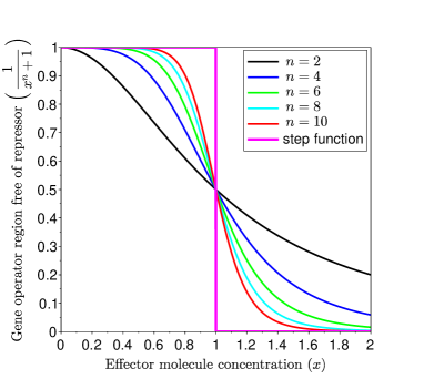
Figure 1: In the case of a repressible enzyme, the fraction of the operator region free of repressor correspond to a monotone decreasing function. The reactions that block transcription occur fast, which in a limit case can be represented as a step function.

For this purpose, we introduce a model that represents local regulation in a metabolic pathway and study its dynamical behavior. The model is based on the end-product control structure introduced in [12] (see also [13]). In this class of local regulation, the metabolite effector is the end product of the pathway and enzyme synthesis of the pathway is induced when the concentration of the effector decreases. In a first stage, we consider that enzyme concentrations remain constant with the purpose of using a slow-fast system approach.

Indeed, the experiments indicate that quasi-steady state exists at the scale of a cell population. However, to assess the stability of metabolic systems is challenging due to the large scale of models and their non-linear dynamics. Even if it is classic in the engineering context to consider that stability is an expected or even necessary property, other behaviors of the system may also be acceptable from the standpoint of the functioning of a dynamic system, as for example the fact that the system oscillates about an average value. Besides, multistability and oscillatory dynamics can emerge in metabolic pathways under gene regulation [6, 9, 46, 34, 5].

In the context of cells, where the stochasticity is very large, fluctuations due to these oscillations would not necessarily be a problem. In this paper, we thus take the counterpart of the classic approach by considering that the negative feedback is high. We will obtain conditions ensuring the existence of an oscillatory regime by considering a limit case, i.e. by assuming that the feedback is an ON/OFF type mechanism.

In Section 2, we describe the model of local regulation. In order to represent the stiffness of allosteric regulation, we consider a deterministic model of a linear metabolic pathway with an input-feedback that switches between two modes (ON and OFF) according to the concentration of the metabolite effector. The fluxes among the metabolites are generalized so that kinetics can be nonlinear, only respecting some monotonicity conditions.

In Section 3, we define a differential inclusion for the switching system following the theory of Filippov for discontinuous systems [8]. We prove that, under some conditions, the solution of the differential inclusion can converge uniformly and asymptotically to an equilibrium point, remain in equilibrium at the sliding mode or oscillate around the sliding mode.

In Section 4, we present an example of a metabolic pathway with Michaelis-Menten reversible reactions. Finally, in Section 5, we show that the solution of the switching system is the limit of function sequences with smooth or piecewise linear inputs that tend towards an ON / OFF type mechanism.

2 Model of local regulation

In this Section we introduce the feedback model studied through the text, which is based on the end-product control structure proposed in [12] (see also [13]). The model corresponds to a metabolic pathway where the end product is the metabolite effector.

We consider the model as a slow-fast system, where metabolites are the fast species and enzymes the slow species. In order to analyze the stability conditions for the fast part of the system according to Tikhonov’s Theorem [20, 22, 40, 43], we assume that enzyme concentrations are constant.

Figure 2: End-product control structure.

The ODE describing the concentration of metabolites in the pathway of Figure 2 is

(1) $$\frac{dX_{1}}{dt} =u(X_{n})-f_{1}(X_{1},X_{2})-\mu\cdot X_{1}$$

$$\frac{dX_{2}}{dt} =f_{1}(X_{1},X_{2})-f_{2}(X_{2},X_{3})-\mu\cdot X_{2}$$

$$\vdots$$

$$\frac{dX_{n}}{dt} =f_{n-1}(X_{n-1},X_{n})-\nu_{n}f_{n}(X_{n})-\mu\cdot X_{n},$$

where $u\colon\mathbb{R}^{n}\to[0,\infty)$ is the input function, $\mu\geq 0$ the growth rate (or decay rate) and $\nu_{n}\geq 0$ an output rate. In this case we consider that allosteric regulation acts on the input flux of the pathway, which can be interpreted as the regulation of the enzyme activity leading to the input by the metabolite effector $X_{n}$ (the end-product of the pathway).

In order to simplify the notation we define

$$f(u,X,\mu,\nu_{n}):=\begin{pmatrix}u(X_{n})-f_{1}(X_{1},X_{2})-\mu\cdot X_{1}\\ f_{1}(X_{1},X_{2})-f_{2}(X_{2},X_{3})-\mu\cdot X_{2}\\ \vdots\\ f_{n-1}(X_{n-1},X_{n})-\nu_{n}f_{n}(X_{n})-\mu\cdot X_{n}\end{pmatrix}.$$

Then, Equation 1 can be rewritten as

$$\frac{dX}{dt}=f(u,X,\mu,\nu_{n}).$$

We assume that kinetics of the metabolic pathway in Figure 2 can be nonlinear, but they respect some monotonicity conditions that are established in Assumption 1. The monotonicity condition implying that functions $f_{i}$ are strictly increasing with respect to the first entry assures the flux from the input to the end-product of the pathway. On the other hand, we consider that reactions can be reversible, but this is not imposed as a condition. Therefore, functions $f_{i}$ are supposed to be decreasing (but not strictly) with respect to the second entry.

Assumption 1.

For every $i=1,\dots,n-1$ assume

• $f_{i}:[0,\infty)\times[0,\infty)\to\mathbb{R}$ and $f_{n}(X_{n}):[0,\infty)\to\mathbb{R}$ are continuous functions,

• $f_{i}(X_{i},X_{i+1})$ is strictly increasing w.r.t. $X_{i}$ and $f_{n}(X_{n})$ is strictly increasing w.r.t. $X_{n}$, i.e.

  $$f_{i}(X_{i},X_{i+1}) <f_{i}(X_{i}^{\prime},X_{i+1}) \forall X_{i}<X_{i}^{\prime},$$

  $$\forall X_{i+1}\in[0,\infty),$$

  $$f_{n}(X_{n}) <f_{n}(X_{n}^{\prime}) \forall X_{n}<X_{n}^{\prime},$$

• $f_{i}(X_{i},X_{i+1})$ is decreasing w.r.t. $X_{i+1}$, i.e.

  $$f_{i}(X_{i},X_{i+1}) \leq f_{i}(X_{i},X^{\prime}_{i+1}) \forall X^{\prime}_{i+1}<X_{i+1},$$

  $$\forall X_{i}\in[0,\infty),$$

• $f_{i}(0,X_{i+1})\leq 0$ for all $X_{i+1}\in[0,\infty)$,

• $f_{i}(X_{i},0)\geq 0$ for all $X_{i}\in[0,\infty)$ and

• and $f_{n}(0)=0$.

3 Hybrid model

We consider the limit case where allosteric regulation can be represented by a step function, which can be understood as the induction or repression of the enzyme activity (see Figure 1). For this purpose, we assume the input of system (1) to be a step function that depends on the concentration of $X_{n}$ the metabolite effector with respect to $K>0$ a threshold value:

(2) $$u[X_{n}]:=\begin{cases}k_{1}&\text{ if }X_{n}<K\\ 0&\text{ if }K<X_{n}\end{cases}.$$

Through the text, we refer to $k_{1}$ as the constant input ON and $0$ as the constant input OFF.

Hence, we suppose that the enzyme activity leading to the input is induced if the concentration of the metabolite effector is under a threshold $K$ (i.e. $X_{n}<K$), and it is repressed when the concentration of the metabolite effector is over the threshold (i.e. $K<X_{n}$).

3.1 Oscillatory system

Switching the input allows to keep the concentration of the metabolite effector $X_{n}$ as close as possible to the threshold $K$. Indeed, the input is OFF when the metabolite effector concentration exceeds the threshold, which allows a decrease of the flux pathway and of $X_{n}$ concentration consequently. Reciprocally, the input is ON if the metabolite effector concentration is under the threshold, which leads to an increment of the flux pathway and $X_{n}$ concentration.

The next Theorem 3.1 states that, if the constant input ON is enough large and the sliding mode is not attained, then the switching leads to an oscillatory behavior in all the states of the system. In [46], the same characteristic was observed for linear monotone tridiagonal systems with nonlinear negative feedback. For the example presented in equation (21) of [46], they have shown that the equilibrium of the system does not satisfy their stability conditions when the effect of the input is lower than a threshold. Then, numerical simulations have put in evidence oscillations in that system with a large value input.

Theorem 3.1.

Under Assumption 1, consider the system

(3) $$\frac{dX}{dt} =f(u[X_{n}],X,\mu,\nu_{n})$$

with initial conditions $X_{i}(t_{0})\geq 0$, $i=1,2,\dots,n$, $K>0$, $k_{1}>0$, $\mu\geq 0$, $\nu_{n}\geq 0$, $\mu+\nu_{n}>0$ and the input $u[X_{n}]$ defined in (2).

Suppose that there exist positive values $Y_{1}^{*},Y_{2}^{*},\dots,Y_{n-1}^{*}$ such that

$$0 =f_{1}(Y_{1}^{*},Y_{2}^{*})-f_{2}(Y_{2}^{*},Y_{3}^{*})-\mu\cdot Y_{2}^{*}$$

$$0 =f_{2}(Y_{2}^{*},Y_{3}^{*})-f_{3}(Y_{3}^{*},Y_{4}^{*})-\mu\cdot Y_{3}^{*}$$

$$\vdots$$

$$0 =f_{n-1}(Y_{n-1}^{*},K)-\nu_{n}f_{n}(K)-\mu\cdot K$$

and that

(4) $$\sum_{i=1}^{n-1}\mu\cdot Y_{i}^{*}+\mu\cdot K+\nu_{n}f_{n}(K)<k_{1}.$$

Then, there is an absolutely continuous function $X=(X_{1},X_{2},\dots,X_{n})$ that satisfies equation (3) for a.e. $t\in[t_{0},\infty)$ and right uniqueness holds in $[t_{0},\infty)\times[0,\infty)^{n}$.

Furthermore, if there is $t^{*}\geq t_{0}$ such that $X_{i}(t^{*})=Y_{i}^{*}$ for every $i=1,2,\dots,n-1$ and $X_{n}(t^{*})=K$, then the switching system (3) remains at sliding mode, i.e., for all $t\geq t^{*}$, $X_{i}(t)=Y_{i}^{*}$ for every $i=1,2,\dots,n-1$ and $X_{n}(t)=K$.

Otherwise, the switching system (3) oscillates around $(Y_{1}^{*},Y_{2}^{*},\dots,Y_{n-1}^{*},K)$. In other words, $X_{i}$ has an oscillatory trajectory that takes the value $Y_{i}^{*}$ infinitely many times for every $i=1,2,\dots,n-1$ and $X_{n}$ has an oscillatory trajectory that takes the value $K$ infinitely many times.

The proof of Theorem 3.1 is in Section 3.3. In the next subsection we present some results necessary to it.

Note 3.2.

To explain the key condition (4), suppose that there exists a constant value $\alpha\cdot k_{1}$ such that the system with constant input

$$\frac{dX}{dt}=f(\alpha\cdot k_{1},X,\mu,\nu_{n})$$

has an equilibrium point $(Y_{1}^{*},Y_{2}^{*},\dots,Y_{n}^{*})$ with $Y_{n}^{*}=K$. Then, by the mass-action kinetics, we have

$$\alpha\cdot k_{1}=\sum_{i=1}^{n-1}\mu\cdot Y_{i}^{*}+\mu\cdot K+\nu_{n}f_{n}(K).$$

This implies by condition (4) that

$$\alpha\cdot k_{1}<k_{1}.$$

In other words, that the input necessary to stabilize $X_{n}$ at $K$ is less than $k_{1}$. In this sense, to have a “large” input $k_{1}$ implies that the switching system oscillates around $(Y_{1}^{*},Y_{2}^{*},\dots,Y_{n-1}^{*},K)$, as an alternative to the stabilization.

Note 3.3.

The sliding mode equilibrium has also been called singular equilibrium in the literature [55, 56, 58, 57]. In [55], an approach to model genetic regulatory networks has been proposed using equations described by piecewise linear functions and differential inclusions. It differs from our approach since we consider hybrid systems with ODEs described by continuous monotonic functions. Moreover, in [55] it is only given the characterization for the stability of singular equilibria, while in this paper the existence of oscillatory regimes is also rigorously proved, which is an important feature for metabolic pathways under genetic regulation. In [56], the stability of cyclic feedback networks with sigmoidal and irreversible kinetics has been studied by means of their Jacobian matrices. Feedback systems are not analyzed in [58, 57], but results on the relationship of stable and periodic solutions of logoid systems and piecewise linear equations are presented in [57] and conditions necessary for the stability of steady states are obtained from a Logoid-Jacobian matrix for gene regulatory networks in [58].

3.2 Systems with constant inputs

To prove Theorem 3.1, it is useful to analyze the metabolic pathway system (1) when the input is a constant function. In this section, we introduce several lemmas for systems with constant inputs that are used in the proof of Theorem 3.1. The proofs of all Lemmas are in Appendix B.

Definition 3.4.

We say that a vector $X=(X_{1},X_{2},\dots,X_{n})\in\mathbb{R}^{n}$ is nonnegative if $X_{i}\geq 0$ for all $i=1,2,\dots,n.$

Similarly, a vector $X=(X_{1},X_{2},\dots,X_{n})\in\mathbb{R}^{n}$ is positive if $X_{i}>0$ for all $i=1,2,\dots,n.$

The next lemma states that, in case of having a nonnegative constant input, system (1) is positively invariant. Moreover, if the system has a nonnegative equilibrium point, this delimits the boundary of some invariant regions.

Lemma 3.5.

Under Assumption 1, consider the system

$$\frac{dX}{dt}=f(\mathbf{I},X,\mu,\nu_{n}),$$

where $\mathbf{I}$ indicates a constant input function with value $\mathbf{I}\geq 0$, $\nu_{n}\geq 0$ and $\mu\geq 0$. Then,

$$\Omega_{1} :=[0,\infty)\times[0,\infty)\times\dots\times[0,\infty)$$

is positively invariant under the flux $X$.

Moreover, suppose that the system above has a nonnegative equilibrium point $X^{*}:=(X_{1}^{*},X_{2}^{*},\dots,X_{n}^{*})$. Then, the subsets

$$\Omega_{2} :=[0,X_{1}^{*}]\times[0,X_{2}^{*}]\times\dots\times[0,X_{n}^{*}],$$

$$\Omega_{3} :=[X_{1}^{*},\infty)\times[X_{2}^{*},\infty)\times\dots\times[X_{n}^{*},\infty),$$

$$\Omega_{4} :=\{X_{1}^{*}\}\times\{X_{2}^{*}\}\times\dots\times\{X_{n}^{*}\},$$

are positively invariant under the flux $X$.

The next proposition claims that if system (1) with a nonnegative constant input has a nonnegative equilibrium point, then, this is globally uniformly asymptotically stable. The proof is divided in two cases. In the case when $\mu>0$, the proof consists on defining a Lyapunov function that is bounded by a positive definite function. Then, using an extension of the LaSalle invariance principle [32], the result is concluded.

In the other case, when $\mu=0$ and $\nu_{n}>0$, the proof follows the ideas of the particular case with Michaelis-Menten kinetics presented in Proposition 8 of [31]. Using that the Jacobian is a column diagonally dominant matrix due to the monotonicity conditions of Assumption 1, it is proved that the equilibrium point is globally attractive and also locally asymptotically stable (see Appendix A).

Proposition 3.6.

Under Assumption 1, consider the system

(5) $$\frac{dX}{dt}=f(\mathbf{I},X,\mu,\nu_{n}),$$

with initial conditions $X_{i}(t_{0})\geq 0$ for every $i=1,2,\dots,n$, the constant input $\mathbf{I}\geq 0$, $\mu\geq 0$, $\nu_{n}\geq 0$ and $0<\mu+\nu_{n}$.

If system (5) has a nonnegative equilibrium point $X^{*}:=(X_{1}^{*},X_{2}^{*},\dots,X_{n}^{*})$, then $X^{*}$ is globally uniformly asymptotically stable (GUAS).

Proof 3.7.

First suppose that $0<\mu$. Define the Lyapunov norm-like function

$$V(X):=\sum_{i=1}^{n}|X_{i}-X_{i}^{*}|,$$

where $X:=(X_{1},X_{2},\dots X_{n})$. The function $V$ is continuous, nonnegative and $V(X)=0$ if and only if $X=X^{*}$ (i.e. $V$ is positive definite).

According to Lemma 3.5, $X_{i}(t)\in[0,\infty)$ for every $t\geq t_{0}$, $i=1,2,\dots,n$. Then, as a consequence of the monotonicity of the functions $f_{i}$ established in Assumption 1 and the existence of the equilibrium point, it follows,

$$\dot{V}(X) =\sum_{i=1}^{n-1}f_{i}(X_{i},X_{i+1})[sgn(X_{i+1}-X_{i+1}^{*})-sgn(X_{i}-X_{i}^{*})]$$

$$+\mathbf{I}\cdot sgn(X_{1}-X_{1}^{*})-\nu_{n}f_{n}(X_{n})\cdot sgn(X_{n}-X_{n}^{*})-\sum_{i=1}^{n}\mu\cdot X_{i}\cdot sgn(X_{i}-X_{i}^{*})$$

$$\leq-\sum_{i=1}^{n-1}\sum_{j=1}^{i}\mu\cdot X_{j}^{*}[sgn(X_{i+1}-X_{i+1}^{*})-sgn(X_{i}-X_{i}^{*})]$$

$$+\sum_{i=1}^{n}\mu\cdot X_{i}^{*}sgn(X_{n}-X_{n}^{*})-\sum_{i=1}^{n}\mu\cdot X_{i}\cdot sgn(X_{i}-X_{i}^{*})$$

$$\leq\sum_{i=1}^{n}\mu\cdot(X_{i}^{*}-X_{i})\cdot sgn(X_{i}-X_{i}^{*})=-\sum_{i=1}^{n}\mu\cdot|X_{i}-X_{i}^{*}|.$$

Defining $W(X):=\sum_{i=1}^{n}\mu\cdot|X_{i}-X_{i}^{*}|$, we have that $W(X)$ is a continuous nonnegative function such that $W(X)=0$ if and only if $X=X^{*}$ and

$$\dot{V}(X) \leq-W(X).$$

Therefore, by means of an extension of LaSalle invariance principle (see Theorem 3.3 in [32]), we conclude that $X^{*}$ is globally uniformly asymptotically stable.

The proof for the case $\mu=0$ and $0<\nu_{n}$ is in Appendix A.

The next Lemma 3.8 states an order for the metabolic pathways with constant inputs. In other words, it compares two systems of the form (1) with constant inputs, according to the input values and their initial conditions.

Moreover, Lemma 3.9 asserts an order for nonnegative equilibrium points of two systems of the form (1) with positive constant inputs.

Finally, Lemma 3.10 states that if a system of the form (1) with constant input has a nonnegative equilibrium point, then there is also a system of the form (1) with a larger constant input that has a larger (entry by entry) equilibrium point.

Lemma 3.8.

Under Assumption 1, consider two systems

$$\frac{dX}{dt} =f(\mathbf{I}_{1},X,\mu,\nu_{n})$$

$$\frac{dY}{dt} =f(\mathbf{I}_{2},Y,\mu,\nu_{n}),$$

with constant inputs that satisfy

$$0\leq\mathbf{I}_{2}\leq\mathbf{I}_{1},$$

$\nu_{n}\geq 0$, $\mu\geq 0$ and initial conditions $X(t_{0})$ and $Y(t_{0})$, respectively, such that

$$0\leq Y_{i}(t_{0}) \leq X_{i}(t_{0}) \forall i=1,2,\dots,n.$$

If $\mathbf{I}_{2}<\mathbf{I}_{1}$, then

$$Y_{i}(t) <X_{i}(t) \forall t\in(t_{0},\infty),\forall i=1,2,\dots,n.$$

Moreover, if $\mathbf{I}_{1}=\mathbf{I}_{2}$ and $Y_{i}(t_{0})<X_{i}(t_{0})$ for every $i=1,2,\dots,n$, there is $T>t_{0}$ such that

$$Y_{i}(t) <X_{i}(t) \forall t\in(t_{0},T),\forall i=1,2,\dots,n,$$

and

$$Y_{i}(t) \leq X_{i}(t) \forall t\in[T,\infty),\forall i=1,2,\dots,n.$$

Lemma 3.9.

Under Assumption 1, consider the following systems

(6) $$\frac{dX}{dt} =f(\mathbf{I}_{1},X,\mu,\nu_{n}),$$

(7) $$\frac{dY}{dt} =f(\mathbf{I}_{2},Y,\mu,\nu_{n}),$$

where $\nu_{n}\geq 0$ and $\mu\geq 0$ and the constant inputs satisfy

$$0\leq\mathbf{I}_{2}<\mathbf{I}_{1}.$$

Suppose that systems (6) and (7) have nonnegative equilibrium points $X^{*}:=(X_{1}^{*},X_{2}^{*},\dots,X_{n}^{*})$ and $Y^{*}:=(Y_{1}^{*},Y_{2}^{*},\dots,Y_{n}^{*})$, respectively. Then,

$$Y_{i}^{*} <X_{i}^{*} \forall i=1,2,\dots,n.$$

Lemma 3.10.

Under Assumption 1, suppose that there is a nonnegative vector $X^{*}:=(X_{1}^{*},X_{2}^{*},\dots,X_{n}^{*})$ such that

$$f(\mathbf{I}_{1},X^{*},\mu,\nu_{n})=\bar{0},$$

with $\mathbf{I}_{1}>0$, $\nu_{n}\geq 0$ and $\mu\geq 0$.

Then, for any $\varepsilon>0$, there exist

$$\mathbf{I}\in(\mathbf{I}_{1},\mathbf{I}_{1}+\varepsilon)$$

and a nonnegative vector $X^{\prime}:=(X_{1}^{\prime},X_{2}^{\prime},\dots,X_{n}^{\prime})$ such that

$$X_{i}^{*} <X_{i}^{\prime} \forall i=1,\dots,n$$

and

$$f(\mathbf{I},X^{\prime},\mu,\nu_{n})=\bar{0}.$$

3.3 Solution existence and right uniqueness

In this section we will prove the existence and right uniqueness of an absolutely continuous solution for the switching system (3). For this purpose, we use the theory of differential inclusions of Filippov [8]. The proofs of all Lemmas are in Appendix B.

Definition 3.11.

We say that for the equation

$$\frac{dx}{dt}=f(t,x)$$

right uniqueness holds at a point $(t_{0},x_{0})$ if there exists $t_{1}>t_{0}$ such that each two solutions of this equation satisfying the condition $x(t_{0})=x_{0}$ coincide on the interval $t_{0}\leq t\leq t_{1}$ or on the part of this interval on which they are both defined. Moreover, right uniqueness holds in a domain $D$ (open or closed) if for each point $(t_{0},x_{0})\in D$ every two solutions satisfying the condition $x(t_{0})=x_{0}$ coincide on each interval $t_{0}\leq t\leq t_{1}$ on which they both exist and lie in this domain [8].

Definition 3.12.

We define the sign as a function $sgn\colon\mathbb{R}\to\{-1,0,1\}$ such that

$$sgn(x):=\begin{cases}-1&\text{if }x<0\\ 0&\text{if }x=0\\ 1&\text{if }x>0\end{cases}.$$

The purpose of Lemma 3.13 and Lemma 3.14 is to analyze the behavior of the switching system (3) when its last state (metabolite $X_{n}$) takes the value $K$ at which the systems switches. This unequivocally defines the value taken by the entry of the switching system (3) in the differential inclusion, allowing to conclude in Proposition 3.15 that right uniqueness holds for its solution.

Lemma 3.13.

Under Assumption 1, consider the system

$$\frac{dX}{dt} =f(\mathbf{I},X,\mu,\nu_{n}),$$

with $\mathbf{I}\geq 0$, $\mu\geq 0$ and $\nu_{n}\geq 0$. Suppose that for some $m\in\{1,2,\dots,n-1\}$

$$\dot{X}_{i}(t_{0}) =0 \forall i>m.$$

Then, there exists $\varepsilon>0$ such that

$$sgn(\dot{X}_{i}(t)) =sgn(\dot{X}_{m}(t)) \forall t\in(t_{0},t_{0}+\varepsilon),\forall i>m.$$

Lemma 3.14.

Under Assumption 1, let $k_{1}>0$, $\mu\geq 0$, $\nu_{n}\geq 0$ and consider the systems

$$\frac{d\widetilde{X}}{dt} =f(k_{1},\widetilde{X},\mu,\nu_{n})$$

$$\frac{dZ}{dt} =f(0,Z,\mu,\nu_{n}),$$

with the same initial conditions

$$\widetilde{X}_{i}(t_{0}) =Z_{i}(t_{0}) \forall i=1,2,\dots,n.$$

Assume that there is $m\in\{2,3,\dots,n\}$ such that

$$\dot{\widetilde{X}}_{m}(t_{0})=\dot{Z}_{m}(t_{0})\not=0.$$

Then, there exists $\varepsilon>0$ such that

$$sgn(\dot{\widetilde{X}}_{n}(t)) =sgn(\dot{Z}_{n}(t)) \forall t\in(t_{0},t_{0}+\varepsilon).$$

Proposition 3.15 (Existence and uniqueness).

Under Assumption 1, consider the system

(8) $$\frac{dX}{dt} =f(u[X_{n}],X,\mu,\nu_{n})$$

with initial conditions $X_{i}(t_{0})\geq 0$, $i=1,2,\dots,n$, $K>0$, $k_{1}>0$, $\mu\geq 0$, $\nu_{n}\geq 0$ and the input $u[X_{n}]$ defined in (2).

Then, there exists an absolutely continuous function $X$ that satisfies (8) for almost every (a.e.) $t\in[t_{0},\infty)$ and right uniqueness holds in $[t_{0},\infty)\times[0,\infty)^{n}$.

Proof 3.16.

Consider the differential inclusion

$$\frac{dX}{dt}\in\mathbf{F}(t,X)$$

with

$$\mathbf{F}(t,X):=\begin{cases}\big{\{}f(k_{1},X,\mu,\nu_{n})\big{\}}&\text{if }X_{n}<K\\ \big{\{}f(0,X,\mu,\nu_{n})\big{\}}&\text{if }K<X_{n}\\ \big{\{}f(\alpha\cdot k_{1},X,\mu,\nu_{n})\colon\alpha\in[0,1]\big{\}}&\text{if }X_{n}=K\end{cases}.$$

For every $(t,X)\in[0,\infty)\times\mathbb{R}^{n}_{+}$, $\mathbf{F}(t,X)$ satisfies the basic conditions [8]: $\mathbf{F}(t,X)$ is nonempty, bounded, closed, convex and upper semi-continuous in $(t,X)$ according to Lemma 3, p. 67 of [8]. Then, by Theorem 1 and Theorem 2, pp. 77-78 of [8], there exists an absolutely continuous function $X$ that satisfies (8) for a.e. $t\in[t_{0},\infty)$.

Right uniqueness follows from the fact that for every $t\in[t_{0},\infty)$ the derivative of an absolutely continuous solution can only take a single value which is given in agreement with the differential inclusion. Indeed, the derivative is uniquely determined in a neighborhood of any $t$ such that $X_{n}(t)\not=K$.

On the other hand, if $X_{n}(t^{\prime})=K$ and there is $m\in\{2,3,\dots,n\}$ such that $\dot{X}_{m}(t^{\prime})\not=0$, by Lemma 3.14, there is only one valid definition for $\dot{X}$ in $(t^{\prime},t^{\prime}+\varepsilon)$, because the options with input $k_{1}$ and $0$ has the same sign in $\dot{X}_{n}$ in $(t^{\prime},t^{\prime}+\varepsilon)$, and therefore, one of this will fail to the restriction regarding the value of $X_{n}$ with respect to $K$. And the option with an input $\alpha\cdot k_{1}$ can only be taken in a complete interval when the system has reached an equilibrium, which cannot be the case since we are supposing $\dot{X}_{m}(t^{\prime})\not=0$.

Finally, if $X_{n}(t^{\prime})=K$ and $\dot{X}_{i}(t^{\prime})=0$ for every $i\in\{2,3,\dots,n\}$, then the system takes the value $Y^{*}$ satisfying $Y_{n}^{*}=K$, which corresponds to the equilibrium of a system with input $\alpha\cdot k_{1}$ for some $\alpha\in\mathbb{R}$. If $1\leq\alpha$, then $\dot{X}_{1}(t^{\prime})\leq 0$ according to Lemma 3.9. Then, by Lemma 3.13, $X_{n}(t)\leq K$ for $t\in(t^{\prime},t^{\prime}+\varepsilon)$ with any of the inputs $k_{1}$ or 0. Therefore, the system takes the mode with input $k_{1}$. If $\alpha\in(0,1)$, the options with inputs $k_{1}$ and 0 fail because

$$0 =\alpha\cdot k_{1}-f_{1}(Y^{*}_{1},Y^{*}_{2})-\mu\cdot Y^{*}_{1}$$

$$<k_{1}-f_{1}(Y^{*}_{1},Y^{*}_{2})-\mu\cdot Y^{*}_{1},$$

$$-f_{1}(Y^{*}_{1},Y^{*}_{2})-\mu\cdot Y^{*}_{1}=-\alpha\cdot k_{1}<0,$$

which, according to Lemma 3.14, means for the system with input $k_{1}$ that $K<X_{n}(t)$ for $t\in(t^{\prime},t^{\prime}+\varepsilon)$ and for the system with input $0$ that $X_{n}(t)<K$ for $t\in(t^{\prime},t^{\prime}+\varepsilon)$, which contradicts the inclusion. Therefore, the systems remains at equilibrium in sliding mode.

In the preceding Proposition 3.15, notice that satisfying the basic conditions given in [8] for every $(t,X)\in[0,\infty)\times\mathbb{R}^{n}_{+}$ allows to define for every $t\in[0,\infty)$ a solution of the differential inclusion

$$\frac{dX}{dt}\in\mathbf{F}(t,X).$$

Finally, we have the elements to prove Theorem 3.1.

Proof 3.17 (Proof of Theorem 3.1).

If there exists $t^{*}\geq t_{0}$ such that $X_{i}(t^{*})=Y_{i}^{*}$ for every $i=1,2,\dots,n$, then the switching system (3) remains at the sliding mode, i.e., $X_{i}(t)=Y_{i}^{*}$ for all $t\geq t^{*}$ (see the proof of Proposition 3.15).

To continue with the proof, without loss of generality, we assume that $X(t)\not=Y^{*}$ for every $t\geq t_{0}$. Consider the ODE systems

(9) $$\frac{d\widetilde{X}}{dt} =f(k_{1},\widetilde{X},\mu,\nu_{n}),$$

(10) $$\frac{dY}{dt} =f(\alpha\cdot k_{1},Y,\mu,\nu_{n}),$$

(11) $$\frac{d\mathcal{X}}{dt} =f(\mathbf{I},\mathcal{X},\mu,\nu_{n}),$$

(12) $$\frac{dZ}{dt} =f(0,Z,\mu,\nu_{n}),$$

where, in agreement with hypothesis (4),

$$\alpha:=\frac{1}{k_{1}}\big{(}\sum_{i=1}^{n-1}\mu\cdot Y_{i}^{*}+\mu\cdot K+\nu_{n}f_{n}(K)\big{)}<1$$

and, by virtue of Lemma 3.10, $\mathbf{I}\in(\alpha\cdot k_{1},k_{1})$ is an input such that system (11) has an equilibrium point $\mathcal{X}^{*}:=(\mathcal{X}_{1}^{*},\dots,\mathcal{X}_{n}^{*})$ satisfying $Y_{i}^{*}<\mathcal{X}_{i}^{*}$ for all $i=1,2,\dots,n-1$ and

(13) $$K<\mathcal{X}_{n}^{*}.$$

Suppose that $X_{n}(t_{0})=K$. Since $X(t_{0})\not=Y^{*}$, as a consequence of Lemma 3.13 and Proposition 3.15, $X_{n}$ either increases or decreases after $t_{0}$. We will suppose that it decreases, i.e. $X_{n}(t)<K$ for $t\in(t_{0},t_{0}+\varepsilon)$ and we will reset the initial condition in such way that $X_{n}(t_{0})<K$ to continue with the demonstration. The reciprocal case when $X_{n}$ increases after $t_{0}$ can be proved analogously.

Hence, let $X_{n}(t_{0})<K$ and consider system (9) and (11) with the same initial conditions, i.e., $\widetilde{X}(t_{0})=\mathcal{X}(t_{0})=X(t_{0})$. According to Proposition 3.6 the equilibrium point $\mathcal{X}^{*}$ is GUAS. Then, (13) implies that there exists $t^{\prime}>t_{0}$ such that

$$K<\mathcal{X}_{n}(t^{\prime}).$$

On the other hand, since $\mathbf{I}<k_{1}$, according to Lemma 3.8, $\widetilde{X}$ upper bounds $\mathcal{X}$. Then,

$$K<\mathcal{X}_{n}(t^{\prime})<\widetilde{X}_{n}(t^{\prime})$$

and we can assure that there exists $t_{1}\in(t_{0},t{\color[rgb]{0,0,0}^{\prime}})$ such that

$$\widetilde{X}_{n}(t) <K \forall t\in(t_{0},t_{1}),$$

$$\widetilde{X}_{n}(t_{1}) =K,$$

(14) $$\widetilde{X}_{n}(t) >K \forall t\in(t_{1},t^{\prime}).$$

Hence, according to Lemma 3.13 and Proposition 3.15,

$$X_{n}(t) =\widetilde{X}_{n}(t) \text{for a.e. }t\in[t_{0},t_{1}].$$

Moreover, by continuity,

$$X_{n}(t_{1}) =\widetilde{X}_{n}(t_{1})=K,$$

$$\dot{X}_{n}(t_{1}) =\dot{\widetilde{X}}_{n}(t_{1})\geq 0.$$

Now consider system (12) with initial condition $Z(t_{1})=X(t_{1})$. Since we have supposed that $X(t)\not=Y^{*}$ for every $t\geq t_{0}$, it follows by Lemma 3.13, Proposition 3.15 and the inequality (14) that

$$K <Z_{n}(t) \forall t\in(t_{1},t_{1}+\varepsilon),$$

$$X_{n}(t) =Z_{n}(t) \text{for a.e. }t\in[t_{1},t_{1}+\varepsilon],$$

for some $\varepsilon>0$. In other words, system (3) has switched at $t_{1}$ and follows the dynamics of system (12) in an interval $[t_{1},t_{1}+\varepsilon]$.

Using similar arguments for the GUAS equilibrium point of system (12), $\bar{0}$, it can be proved that system (3) switches at a point $t_{2}>t_{1}$ and returns to the dynamics of (9). The oscillatory behavior of $X_{i}$ around $Y_{i}^{*}$ for $i=1,2,\dots,n-1$ can be proved by induction using as induction hypothesis that $X_{j}$ oscillates around $Y_{j}^{*}$ for every $j=i+1,\dots,n-1$ and $X_{n}$ oscillates around $K$.

3.4 Stable system

In this Section, we present and prove Theorem 3.18 that states some conditions under which the switching system (15) converges uniformly and asymptotically to an equilibrium point.

The switching systems (3) and (15) are the same, but in Theorem 3.18 we consider that the constant input ON is equal to or lower than the threshold value also considered in Theorem 3.1. Or that this threshold is not defined (because there is not a positive sliding mode) and that the system with the constant input ON has a nonnegative equilibrium point.

Theorem 3.18.

Under Assumption 1, consider the switching system

(15) $$\frac{dX}{dt} =f(u[X_{n}],X,\mu,\nu_{n})$$

with initial conditions $X_{i}(t_{0})\geq 0$, $i=1,2,\dots,n$, $K>0$, $k_{1}>0$, $\mu\geq 0$, $\nu_{n}\geq 0$, $\mu+\nu_{n}>0$ and the input $u[X_{n}]$ defined in (2). Consider the system with constant input ON

(16) $$\frac{d\widetilde{X}}{dt} =f(k_{1},\widetilde{X},\mu,\nu_{n}).$$

Suppose that one of the following conditions is satisfied:

• There exist positive values $Y_{1}^{*},Y_{2}^{*},\dots,Y_{n-1}^{*}$ such that

  $$0 =f_{1}(Y_{1}^{*},Y_{2}^{*})-f_{2}(Y_{2}^{*},Y_{3}^{*})-\mu\cdot Y_{2}^{*}$$

  $$0 =f_{2}(Y_{2}^{*},Y_{3}^{*})-f_{3}(Y_{3}^{*},Y_{4}^{*})-\mu\cdot Y_{3}^{*}$$

  $$\vdots$$

  $$0 =f_{n-1}(Y_{n-1}^{*},K)-\nu_{n}f_{n}(K)-\mu\cdot K,$$

  and

  $$k_{1}\leq\sum_{i=1}^{n-1}\mu\cdot Y_{i}^{*}+\mu\cdot K+\nu_{n}f_{n}(K).$$

• There are not positive values $Y_{1}^{*},Y_{2}^{*},\dots,Y_{n-1}^{*}$ such that

  $$0 =f_{1}(Y_{1}^{*},Y_{2}^{*})-f_{2}(Y_{2}^{*},Y_{3}^{*})-\mu\cdot Y_{2}^{*}$$

  $$0 =f_{2}(Y_{2}^{*},Y_{3}^{*})-f_{3}(Y_{3}^{*},Y_{4}^{*})-\mu\cdot Y_{3}^{*}$$

  $$\vdots$$

  $$0 =f_{n-1}(Y_{n-1}^{*},K)-\nu_{n}f_{n}(K)-\mu\cdot K,$$

  and the system with constant input (16) has a nonnegative equilibrium point $\widetilde{X}^{*}:=(\widetilde{X}_{1}^{*},\widetilde{X}_{2}^{*},\dots,\widetilde{X}_{n}^{*})$.
  

Then, there is an absolutely continuous solution $X=(X_{1},X_{2},\dots,X_{n})$ that satisfies equation (15) for a.e. $t\in(t_{0},\infty)$ and right uniqueness holds in $[t_{0},\infty)\times[0,\infty)^{n}$.

Furthermore, supposing that i) is satisfied, if there is $t^{*}\geq t_{0}$ such that $X_{i}(t^{*})=Y_{i}^{*}$ for every $i=1,2,\dots,n-1$ and $X_{n}(t^{*})=K$, then the switching system (15) remains at sliding mode, i.e., $X_{i}(t)=Y_{i}^{*}$ for every $i=1,2,\dots,n-1$ and $X_{n}(t)=K$ for all $t\geq t^{*}$. Otherwise, the system with constant input (16) has a nonnegative equilibrium point $\widetilde{X}^{*}:=(\widetilde{X}_{1}^{*},\widetilde{X}_{2}^{*},\dots,\widetilde{X}_{n}^{*})$ and $\widetilde{X}^{*}$ is globally uniformly asymptotically stable (GUAS) for the switching system (15).

On the other hand, if ii) is satisfied, $\widetilde{X}^{*}$ is globally uniformly asymptotically stable (GUAS) for the switching system (15).

Note 3.19.

Under the conditions of Theorem 3.18, the switching system (15) can converge to the equilibrium point $Y^{*}:=(Y_{1}^{*},Y_{2}^{*},\dots,Y^{*}_{n-1},K)$ corresponding to the sliding mode in two different ways. In one case, it converges in finite time to $Y^{*}$ when there is $t^{*}\geq t_{0}$ such that $X_{i}(t^{*})=Y_{i}^{*}$ for all $i=1,2,\dots,n-1$ and $X_{n}(t^{*})=K$ (we then say that it remains at sliding mode). In the other case, it converges asymptotically to $Y^{*}$ when $k_{1}=\sum_{i=1}^{n-1}\mu\cdot Y_{i}^{*}+\mu\cdot K+\nu_{n}f_{n}(K)$, because this implies that $Y^{*}=\widetilde{X}^{*}$, where $\widetilde{X}^{*}$ is the equilibrium point of the system with the constant input ON (16).

The proof of Theorem 3.18 is given at the end of this section. The following Lemma 3.20 allows to prove in Theorem 3.18 that the system of the form (1) and the constant input ON has an equilibrium point lower or equal (entry by entry) to the equilibrium point corresponding to the sliding mode of the switching system (15).

On the other hand, in Lemma 3.21 it is shown that the switching system is bounded by any system of the form (1) with constant input larger or equal to the constant input ON. The proofs of all Lemmas are in Appendix B.

Lemma 3.20.

Under Assumption 1, suppose that there is a positive vector $X^{*}:=(X_{1}^{*},X_{2}^{*},\dots,X_{n}^{*})$ ($0<X_{i}^{*}$ for all $i=1,\dots,n$) such that

$$0 =f_{1}(X^{*}_{1},X^{*}_{2})-f_{2}(X^{*}_{2},X^{*}_{3})-\mu\cdot X^{*}_{2}$$

$$0 =f_{2}(X^{*}_{2},X^{*}_{3})-f_{2}(X^{*}_{3},X^{*}_{4})-\mu\cdot X^{*}_{3}$$

$$\vdots$$

$$0 =f_{n-1}(X^{*}_{n-1},X^{*}_{n})-\nu_{n}f_{n}(X^{*}_{n})-\mu\cdot X^{*}_{n},$$

with $\mu\geq 0$, $\nu_{n}\geq 0$.

Then, for any $X_{n}^{\prime}\in(0,X_{n}^{*})$, there are unique $X_{1}^{\prime},X_{2}^{\prime},\dots,X_{n-1}^{\prime}$ such that $0\leq X_{i}^{\prime}<X_{i}^{*}$, for all $i=1,2,\dots,n$, and

$$0 =f_{1}(X^{\prime}_{1},X^{\prime}_{2})-f_{2}(X^{\prime}_{2},X^{\prime}_{3})-\mu\cdot X^{\prime}_{2}$$

$$0 =f_{2}(X^{\prime}_{2},X^{\prime}_{3})-f_{2}(X^{\prime}_{3},X^{\prime}_{4})-\mu\cdot X^{\prime}_{3}$$

$$\vdots$$

$$0 =f_{n-1}(X^{\prime}_{n-1},X^{\prime}_{n})-\nu_{n}f_{n}(X^{\prime}_{n})-\mu\cdot X^{\prime}_{n},$$

Lemma 3.21.

Under Assumption 1, consider the switching system

$$\frac{dX}{dt} =f(u[X_{n}],X,\mu,\nu_{n}),$$

with initial conditions $X_{i}(t_{0})\geq 0$, $i=1,2,\dots,n$, $K>0$, $k_{1}>0$, $\mu\geq 0$, $\nu_{n}\geq 0$ and the input $u[X_{n}]$ defined in (2).

Then, the system

$$\frac{d\widetilde{X}}{dt} =f(\mathbf{I},\widetilde{X},\mu,\nu_{n}),$$

with constant input $\mathbf{I}\geq k_{1}$ and initial conditions $\widetilde{X}(t_{0})=X(t_{0})$, is an upper bound of the switching system, i.e.,

$$X_{i}(t) \leq\widetilde{X}_{i}(t) \forall t_{0}\leq t,\forall i=1,2,\dots,n.$$

Moreover, the system

$$\frac{dZ}{dt} =f(0,Z,\mu,\nu_{n}),$$

with constant input $0<k_{1}$ and initial conditions $Z(t_{0})=X(t_{0})$, is a lower bound of the switching system, i.e.,

$$Z_{i}(t) \leq X_{i}(t) \forall t_{0}\leq t,\forall i=1,2,\dots,n.$$

Note 3.22.

Lemma 3.21 can also be applied to the switching system of Theorem 3.1.

There are now all the components necessaries to prove Theorem 3.18.

Proof 3.23 (Proof of Theorem 3.18).

The existence and uniqueness of the solution follow by Proposition 3.15. To prove that $\widetilde{X}^{*}$ is GUAS for the switching system (15), we first consider the case where i) is satisfied. Define

$$\alpha:=\frac{1}{k_{1}}\big{(}\sum_{i=1}^{n-1}\mu\cdot Y_{i}^{*}+\mu\cdot K+\nu_{n}f_{n}(K)\big{)}.$$

Notice that $1\leq\alpha$. First suppose that $1<\alpha$ and consider the system

(17) $$\frac{dY}{dt} =f(\alpha\cdot k_{1},Y,\mu,\nu_{n}),$$

which has the positive equilibrium point $Y^{*}:=(Y_{1}^{*},Y_{2}^{*},\dots,Y_{n-1}^{*},K)$. By Proposition 3.6, $Y^{*}$ is globally uniformly asymptotically stable (GUAS) for (17). Moreover, system (16) has also an equilibrium point $\widetilde{X}^{*}$ according to Lemma 3.20, because $k_{1}<\alpha\cdot k_{1}$. Moreover, by Lemma 3.8,

$$\widetilde{X}_{i}(t) <Y_{i}(t) \forall t_{0}\leq t,\forall i=1,2,\dots,n,$$

$\widetilde{X}^{*}$ is a GUAS equilibrium point for system (16) by Proposition 3.6 and $\widetilde{X}_{n}^{*}<K$ by Lemma 3.9. Then,there exists $T\geq t_{0}$ large enough such that

$$\widetilde{X}_{n}(t) <K \forall t\geq T.$$

On the other hand, according to Lemma 3.21, the switching system (15) is bounded by the system with constant input (16). That is to say,

$$X_{i}(t) \leq\widetilde{X}_{i}(t) \forall t_{0}\leq t,\forall i=1,2,\dots,n.$$

Therefore,

$$X_{i}(t) \leq\widetilde{X}_{n}(t)<K \forall T\leq t.$$

Then, the switching system (15) is in the regime of the system with constant input (16) in the interval $[T,\infty)$. Therefore, $\widetilde{X}^{*}$ is a GUAS equilibrium point for the switching system (15).

For the case $\alpha=1$, suppose there is not $t^{\prime}\geq t_{0}$ such that $X_{n}(t)\leq K$ for all $t\geq t^{\prime}$. Then it can be proved that the switching system (15) oscillates around the sliding mode $(Y_{1}^{*},Y_{2}^{*},\dots,Y_{n-1}^{*},K)$ (in a similar way as in Theorem 3.1). This implies the existence of $t^{\prime\prime}\geq t_{0}$ such that $X_{i}(t^{\prime\prime})\leq Y_{i}^{*}$ for every $i=1,2,\dots,n-1$ and $X_{n}(t^{\prime\prime})\leq K$. But according to Lemma 3.5, system (16) is invariant in $[0,Y_{1}^{*}]\times[0,Y_{2}^{*}]\times\dots\times[0,Y_{n-1}^{*}]\times[0,K]$, because $\widetilde{X}_{i}^{*}=Y_{i}^{*}$ for $i=1,2,\dots,n-1$ and $\widetilde{X}^{*}=K$. Hence, $X_{n}(t)\leq K$ for every $t\geq t^{\prime\prime}$, which contradicts our supposition.

We conclude that, when $\alpha=1$, there is $t^{\prime}\geq t_{0}$ such that $X_{n}(t)\leq K$ for all $t\geq t^{\prime}$. Then the switches system (15) follows the regime of system (16) and converges to the sliding mode $(Y_{1}^{*},Y_{2}^{*},\dots,Y_{n-1}^{*},K)$, which is equal to the equilibrium point $\widetilde{X}^{*}$ of system (16).

Now suppose that point i) is not satisfied. Then, point ii) holds by hypothesis. Moreover, $\widetilde{X}_{n}^{*}<K$ according to Lemma 3.20. Hence, there exists $T\geq t_{0}$ large enough such that $\widetilde{X}_{n}(t)<K$ for every $t\geq T$. But, by Lemma 3.21, the switching system (15) is bounded by the system with constant input $k_{1}$ (16), i.e.

$$X_{i}(t) \leq\widetilde{X}_{i}(t) \forall t_{0}\leq t.$$

In particular,

$$X_{n}(t) \leq\widetilde{X}_{n}(t)<K \forall T\leq t.$$

Therefore, the switching system (15) has the dynamics of system (16) in the interval $[T,\infty)$ and converges uniformly and asymptotically to $\widetilde{X}^{*}$.

Note 3.24.

In this section we have presented results for a system where all the states have the same decay rate. A generalization of these results can be achieved considering different decay rates. This can be useful in the context of gene networks, where very distinct degradation rates are involved [52, 54].

We can then enunciate a more general result as follows:

Theorem 3.25.

Under Assumption 1, consider the system

(18) $$\frac{dX_{1}}{dt} =u[X_{n}]-f_{1}(X_{1},X_{2})-\mu_{1}\cdot X_{1}$$

$$\frac{dX_{2}}{dt} =f_{1}(X_{1},X_{2})-f_{2}(X_{2},X_{3})-\mu_{2}\cdot X_{2}$$

$$\vdots$$

$$\frac{dX_{n}}{dt} =f_{n-1}(X_{n-1},X_{n})-\nu_{n}f_{n}(X_{n})-\mu_{n}\cdot X_{n},$$

with initial conditions $X_{i}(t_{0})\geq 0$, $i=1,2,\dots,n$, $K>0$, $k_{1}>0$, $\mu_{i}\geq 0$ for all $i=1,2,\dots,n$, $\nu_{n}\geq 0$, $\mu_{n}+\nu_{n}>0$ and the input $u[X_{n}]$ defined in (2).

Suppose that there exist positive values $Y_{1}^{*},Y_{2}^{*},\dots,Y_{n-1}^{*}$ such that

(19) $$0 =f_{1}(Y_{1}^{*},Y_{2}^{*})-f_{2}(Y_{2}^{*},Y_{3}^{*})-\mu_{2}\cdot Y_{2}^{*}$$

$$0 =f_{2}(Y_{2}^{*},Y_{3}^{*})-f_{3}(Y_{3}^{*},Y_{4}^{*})-\mu_{3}\cdot Y_{3}^{*}$$

$$\vdots$$

$$0 =f_{n-1}(Y_{n-1}^{*},K)-\nu_{n}f_{n}(K)-\mu_{n}\cdot K$$

and define

$$\alpha:=\frac{\sum_{i=1}^{n-1}\mu_{i}\cdot Y_{i}^{*}+\mu_{n}\cdot K+\nu_{n}f_{n}(K)}{k_{1}}.$$

Then, there is an absolutely continuous function $X=(X_{1},X_{2},\dots,X_{n})$ that satisfies equation (18) for a.e. $t\in[t_{0},\infty)$ and right uniqueness holds in $[t_{0},\infty)\times[0,\infty)^{n}$.

Furthermore, if there is $t^{*}\geq t_{0}$ such that $X_{i}(t^{*})=Y_{i}^{*}$ for every $i=1,2,\dots,n-1$ and $X_{n}(t^{*})=K$, then the switching system (18) remains at sliding mode, i.e., for all $t\geq t^{*}$, $X_{i}(t)=Y_{i}^{*}$ for every $i=1,2,\dots,n-1$ and $X_{n}(t)=K$.

Otherwise,

• if $\alpha<1$, the switching system (18) oscillates around $(Y_{1}^{*},Y_{2}^{*},\dots,Y_{n-1}^{*},K)$,

• if $1\leq\alpha$, the system with constant input

  (20) $$\frac{d\widetilde{X}_{1}}{dt} =k_{1}-f_{1}(\widetilde{X}_{1},\widetilde{X}_{2})-\mu_{1}\cdot\widetilde{X}_{1}$$

  $$\frac{d\widetilde{X}_{2}}{dt} =f_{1}(\widetilde{X}_{1},\widetilde{X}_{2})-f_{2}(\widetilde{X}_{2},\widetilde{X}_{3})-\mu_{2}\cdot\widetilde{X}_{2}$$

  $$\vdots$$

  $$\frac{d\widetilde{X}_{n}}{dt} =f_{n-1}(\widetilde{X}_{n-1},\widetilde{X}_{n})-\nu_{n}f_{n}(\widetilde{X}_{n})-\mu_{n}\cdot\widetilde{X}_{n},$$

  has a nonnegative equilibrium point $\widetilde{X}^{*}$ and $\widetilde{X}^{*}$ is globally uniformly asymptotically stable (GUAS) for the switching system (18).
  

If such positive values $Y_{1}^{*},Y_{2}^{*},\dots,Y_{n-1}^{*}$ satisfying (19) do not exist and system (20) has a nonnegative equilibrium point $\widetilde{X}^{*}$, then $\widetilde{X}^{*}$ is globally uniformly asymptotically stable (GUAS) for the switching system (18).

The proof of Theorem 3.25 can be obtained following the proofs for Theorem 3.1 and Theorem 3.18, and substituting $\mu\cdot X_{i}$, $\mu\cdot Y_{i}$, etc, for $\mu_{i}\cdot X_{i}$, $\mu_{i}\cdot Y_{i}$, etc, respectively.

Note 3.26.

According to the definition given in [46], system (1) can be considered as a tridiagonal feedback system provided that $u$ and $f_{i}$ are of class $C^{1}$ for all $i=1,2,\dots,n$. Theorems 1 and 2 in [46] give conditions to prove global asymptotic stability of an equilibrium point for tridiagonal feedback systems. These conditions imply the existence of a compact absorbing subset of the domain (i.e. an invariant compact set) and a Metzler and Hurwitz matrix that upper bounds the Jacobian matrix of the system or a second compound matrix. The examples of linear monotone tridiagonal systems with nonlinear negative feedback and the Goldbeter model are also used in [46] to exhibit oscillations in tridiagonal monotone systems when the conditions for stability fail.

Contrary to the differentiability condition required in [46], we consider a non continuous differential equation by assuming a negative feedback that is piecewise constant and discontinuous (see definition (2)). Our approach allows to obtain conditions to prove not only global uniform asymptotic stability of equilibrium points (Theorem 3.18), but also sliding mode and oscillatory regimes (Theorem 3.1). Moreover, these conditions are equivalent to solve an algebraic equation to find equilibria, which in case of mass-action kinetics is often feasible.

4 Example with Michaelis-Menten reversible reactions

We show an example of the switching system (3) (or system (15)) with 3 metabolites and Michaelis-Menten reversible reactions. Let

$$u[X_{3}] :=\begin{cases}k_{1}&\text{ if }X_{3}<K\\ 0&\text{ if }K<X_{3}.\end{cases}$$

$$f_{1}(X_{1},X_{2}) :=\frac{k_{2}X_{1}-l_{2}X_{2}}{m_{2}X_{1}+n_{2}X_{2}+K_{2}},$$

$$f_{2}(X_{2},X_{3}) :=\frac{k_{3}X_{2}-l_{3}X_{3}}{m_{3}X_{2}+n_{3}X_{3}+K_{3}},$$

$$f_{3}(X_{3}) :=\nu_{n}\frac{X_{3}}{X_{3}+K_{n}},$$

$$f(u,X,\mu,\nu_{n}):= \begin{pmatrix}u-f_{1}(X_{1},X_{2})-\mu X_{1}\\ f_{1}(X_{1},X_{2})-f_{2}(X_{2},X_{3})-\mu X_{2}\\ f_{2}(X_{2},X_{3})-\nu_{n}f_{3}(X_{3})-\mu X_{3}\end{pmatrix},$$

for some $k_{1}>0$, $K>0$, $\mu\geq 0$, $\nu_{n}\geq 0$ and $0<\mu+\nu_{n}$.

Consider the ODE systems

(21) $$\frac{dX}{dt} =f(u[X_{3}],X,\mu,\nu_{n}),$$

(22) $$\frac{d\widetilde{X}}{dt} =f(k_{1},\widetilde{X},\mu,\nu_{n}),$$

(23) $$\frac{dY}{dt} =f(\alpha\cdot k_{1},Y,\mu,\nu_{n}),$$

(24) $$\frac{dZ}{dt} =f(0,Z,\mu,\nu_{n}),$$

where

$$\alpha:=\frac{1}{k_{1}}\big{(}\sum_{i=1}^{n-1}\mu\cdot Y_{i}^{*}+\mu\cdot K+\nu_{n}f_{n}(K)\big{)}.$$

4.1 Oscillatory system

Figure 3 and Figure 4 show two examples of the oscillatory behavior described in Theorem 3.1. In both cases, the constant input ON of the switching system (21) is larger enough to satisfy the inequality in (4). Moreover, we observe that the solution of the switching system (21) is bounded between the solution of system (22) with the constant input ON and the solution of system (24) with the constant input OFF, as stated in Lemma 3.21.

Notice that even when system (22) with the constant input ON has no positive equilibrium point, the switching system (21) oscillates around the sliding mode (see Figure 4).

On the other hand, in Appendix C we present an example to compare the dynamics of a piecewise linear model and a hybrid model as (3). The example shows oscillations in both cases for a pathway with irreversible kinetics.

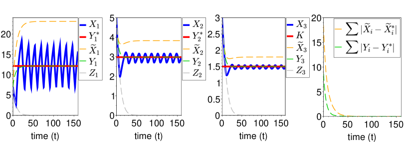
Figure 3: Solution for systems (21)-(24) and candidate Lyapunov function for (22) and (23). All parameters are equal to $1$ except for $k_{1}=3$, $\nu_{n}=0.2$, $\mu=0.1$ and $K=1.5$. The initial conditions are $X_{1}(0)=7$, $X_{2}(0)=5$ and $X_{3}(0)=3$. The switching system (21) oscillates around the sliding mode $(Y_{1}^{*},Y_{2}^{*},K)$, which is the equilibrium point of system (23). Moreover, the switching system (21) is bounded between systems (22) and (24), which converge both to their respective equilibrium points.

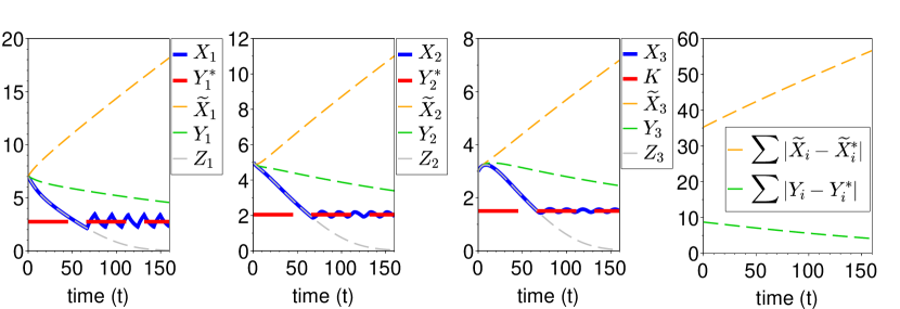
Figure 4: Solution for systems (21)-(24) and candidate Lyapunov function for (22) and (23). All parameters are equal to $1$ except for $k_{1}=0.3$, $\nu_{n}=0.2$, $\mu=0$ and $K=1.5$. The initial conditions are $X_{1}(0)=7$, $X_{2}(0)=5$ and $X_{3}(0)=3$. The switching system (21) oscillates around the sliding mode $(Y_{1}^{*},Y_{2}^{*},K)$, which is the equilibrium point of system (23). Moreover, the switching system (21) is bounded between systems (22) and (24). However, system (22) does not have a positive equilibrium point and it is not stable.. System (24) converges to $\bar{0}$.

4.2 Stable system

In Figure 5, Figure 6 and Figure 7 there are three examples of the stabilization of the switching system (21) as stated in Theorem 3.18.

Figure 5 depicts the case when system (23) with constant input $\alpha\cdot k_{1}$ has a positive equilibrium point and $1<\alpha$ (i.e. i) is satisfied). In this case, the constant input ON is small enough to let the system stabilize and do not oscillate around the sliding mode. Notice that the equilibrium point of the switching system (21) is uniformly asymptotically stable and lower (entry by entry) than the equilibrium point related to the sliding mode (i.e. $Y^{*}$ the equilibrium point of system (23)).

In Figure 6, condition i) is not satisfied, but ii) holds. That is to say, the system related to the sliding mode (23) has not a nonnegative equilibrium point (it has an equilibrium point, but its first entry is negative) and system (22) with the constant input ON has a positive equilibrium point. In this case, the switching system (21) converges uniformly and asymptotically to the equilibrium point of system (22).

The case when the switching system (21) reaches the sliding mode is represented in Figure 7. Here the constant input ON is such that system (22) has an equilibrium point satisfying $\widetilde{X}_{n}^{*}=K$. The switching system (21) converges uniformly and asymptotically to the sliding mode $Y^{*}=\widetilde{X}^{*}$.

Finally, as stated in Lemma 3.21, in the three examples it can be observed that the solution of the switching system (21) is upper and lower bounded by system (22) and system (24), the solutions of the systems with the constant inputs ON and OFF, respectively.

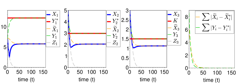
Figure 5: Solution for systems (21)-(24) and candidate Lyapunov function for (22) and (23). All parameters are equal to $1$ except for $\nu_{n}=0.2$, $\mu=0.1$ and $K=1.5$. The initial conditions are $X_{1}(0)=7$, $X_{2}(0)=5$ and $X_{3}(0)=3$. The switching system (21) converges to the equilibrium point of system (22), because $k_{1}<\alpha\cdot k_{1}$. Moreover, the switching system (21) is bounded between systems (22) and (24), which converge both to their respective equilibrium points. System (23) converges to its positive equilibrium point $(Y_{1}^{*},Y_{2}^{*},K)$.

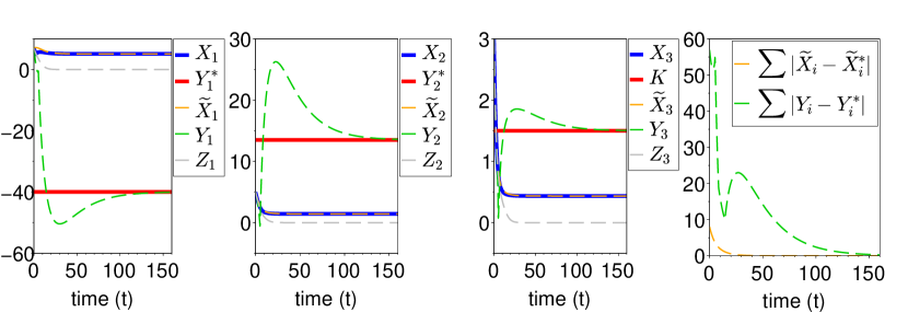
Figure 6: Solution for systems (21)-(24) and candidate Lyapunov function for (22) and (23). All parameters are equal to $1$ except for $\mu=0.1$ and $K=1.5$. The initial conditions are $X_{1}(0)=7$, $X_{2}(0)=5$ and $X_{3}(0)=3$. The switching system (21) converges to the equilibrium point of system (22), because $\alpha<1$. Moreover, the switching system (21) is bounded between systems (22) and (24), which converge both to their respective equilibrium points. The equilibrium point $(Y_{1}^{*},Y_{2}^{*},K)$ of system (23) is nonpositive.

Figure 7: Solution for systems (21)-(24) and candidate Lyapunov function for (22) and (23). All parameters are equal to $1$ except for $k_{1}=\mu\cdot(Y_{1}^{*}+Y_{2}^{*}+K)+\nu_{n}f_{n}(K)\sim 1.78$, $\nu_{n}=0.2$, $\mu=0.1$ and $K=1.5$. The initial conditions are $X_{1}(0)=7$, $X_{2}(0)=5$ and $X_{3}(0)=3$. The switching system (21) converges asymptotically to the sliding mode, which is the equilibrium point of systems (22) and (23), because $\alpha=1$. Moreover, the switching system (21) is bounded between systems (22) and (24), which converge both to their respective equilibrium points.

4.3 Example with different decay rates

We show an example of a system with different decay rates to illustrate Theorem 3.25. As in the previous example, we consider reversible Michaelis-Menten kinetics. Let

$$u[X_{3}] :=\begin{cases}k_{1}&\text{ if }X_{3}<K\\ 0&\text{ if }K<X_{3}.\end{cases}$$

$$f_{1}(X_{1},X_{2}) :=\frac{k_{2}X_{1}-l_{2}X_{2}}{m_{2}X_{1}+n_{2}X_{2}+K_{2}},$$

$$f_{2}(X_{2},X_{3}) :=\frac{k_{3}X_{2}-l_{3}X_{3}}{m_{3}X_{2}+n_{3}X_{3}+K_{3}},$$

$$f_{3}(X_{3}) :=\nu_{n}\frac{X_{3}}{X_{3}+K_{n}},$$

$$g(u,X,\overline{\mu},\nu_{n}):= \begin{pmatrix}u-f_{1}(X_{1},X_{2})-\mu_{1}X_{1}\\ f_{1}(X_{1},X_{2})-f_{2}(X_{2},X_{3})-\mu_{2}X_{2}\\ f_{2}(X_{2},X_{3})-\nu_{n}f_{3}(X_{3})-\mu_{3}X_{3}\end{pmatrix},$$

for some $k_{1}>0$, $K>0$, $\mu_{i}\geq 0$ for all $i=1,2,3$, $\nu_{n}\geq 0$ and $0<\mu_{3}+\nu_{n}$.

Consider the ODE systems

(25) $$\frac{dX}{dt} =g(u[X_{3}],X,\overline{\mu},\nu_{n}),$$

(26) $$\frac{d\widetilde{X}}{dt} =g(k_{1},\widetilde{X},\overline{\mu},\nu_{n}),$$

(27) $$\frac{dY}{dt} =g(\alpha\cdot k_{1},Y,\overline{\mu},\nu_{n}),$$

(28) $$\frac{dZ}{dt} =g(0,Z,\overline{\mu},\nu_{n}),$$

where

$$\alpha:=\frac{1}{k_{1}}\big{(}\sum_{i=1}^{n-1}\mu_{i}\cdot Y_{i}^{*}+\mu_{n}\cdot K+\nu_{n}f_{n}(K)\big{)}.$$

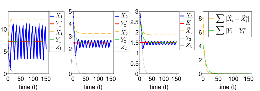
Figure 8: Solution for systems (25)-(28) with different decay rates and candidate Lyapunov function for (26) and (27). All parameters are equal to $1$ except for $k_{1}=3$, $\nu_{n}=0.2$, $\mu_{1}=0.2$, $\mu_{2}=0.1$, $\mu_{3}=0.05$ and $K=1.5$. The initial conditions are $X_{1}(0)=7$, $X_{2}(0)=5$ and $X_{3}(0)=3$. The switching system (25) oscillates around the sliding mode $(Y_{1}^{*},Y_{2}^{*},K)$, which is the equilibrium point of system (27). Moreover, the switching system (25) is bounded between systems (26) and (28), which converge both to their respective equilibrium points.

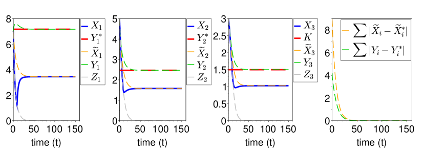
Figure 9: Solution for systems (25)-(28) with different decay rates and candidate Lyapunov function for (26) and (27). All parameters are equal to $1$ except for $\nu_{n}=0.2$, $\mu_{1}=0.2$, $\mu_{2}=0.1$, $\mu_{3}=0.05$ and $K=1.5$. The initial conditions are $X_{1}(0)=7$, $X_{2}(0)=5$ and $X_{3}(0)=3$. The initial conditions are $X_{1}(0)=7$, $X_{2}(0)=5$ and $X_{3}(0)=3$. The switching system (25) converges to the equilibrium point of system (26), because $k_{1}<\alpha\cdot k_{1}$. Moreover, the switching system (25) is bounded between systems (26) and (28), which converge both to their respective equilibrium points. System (27) converges to its positive equilibrium point $(Y_{1}^{*},Y_{2}^{*},K)$.

Figure 10: Solution for systems (25)-(28) with different decay rates and candidate Lyapunov function for (26) and (27). All parameters are equal to $1$ except for $k_{1}=\mu_{1}\cdot Y_{1}^{*}+\mu_{2}\cdot Y_{2}^{*}+\mu_{3}\cdot K+\nu_{n}f_{n}(K)\sim 1.88$, $\nu_{n}=0.2$, $\mu_{1}=0.2$, $\mu_{2}=0.1$, $\mu_{3}=0.05$ and $K=1.5$. The initial conditions are $X_{1}(0)=7$, $X_{2}(0)=5$ and $X_{3}(0)=3$. The switching system (25) converges asymptotically to the sliding mode, which is the equilibrium point of systems (26) and (27), because $\alpha=1$. Moreover, the switching system (25) is bounded between systems (26) and (28), which converge both to their respective equilibrium points.

5 Continuous feedback systems

The purpose of this Section is to exhibit some sequences of equations of the form (1) with continuous inputs whose solutions converge pointwise to the solution of the switching system (3) (equal to system (15)). This follows the idea of considering the switching input (2) as the limit case of allosteric regulation processes that occur very fast (see Section 1 and Figure 1).

5.1 Smooth input

In Proposition 5.1, we introduce a sequence of equations of the form (1) with smooth inputs. The purpose is that the smooth inputs converge to the step function defined by the switching input (2). For this, sigmoid functions of the form

$$\frac{k_{1}}{1+\big{(}\frac{X_{n}}{K}\big{)}^{m}}$$

are considered. However, a sigmoid input would not allow the system to remain constant in the sliding mode if there is $t^{*}\geq t_{0}$ such that $X_{i}(t^{*})=Y_{i}^{*}$ for every $i=1,2,\dots,n-1$ and $X_{n}(t^{*})=K$. This is a property that, according to Theorem 3.1 and Theorem 3.18, the switching systems (3) and (15) satisfy. In order to approximate this particular dynamics of the switching systems, the sigmoid function is multiplied by the Gaussian function

$$\Big{[}(2\cdot\alpha-1)\cdot\exp\Big{\{}-\Big{(}\frac{X_{n}-K}{\sigma}\Big{)}^{2}\Big{\}}+1\Big{]}.$$

Proposition 5.1.

Under Assumption 1, consider the switching system

$$\frac{dX}{dt} =f(u[X_{n}],X,\mu,\nu_{n})$$

with initial conditions $X_{i}(t_{0})\geq 0$, $i=1,2,\dots,n$, $K>0$, $k_{1}>0$, $\mu\geq 0$, $\nu_{n}\geq 0$ and the input $u[X_{n}]$ defined in (2).

Suppose that there are positive values $Y_{1}^{*},Y_{2}^{*},\dots,Y_{n-1}^{*}$ such that

$$0 =f_{1}(Y_{1}^{*},Y_{2}^{*})-f_{2}(Y_{2}^{*},Y_{3}^{*})-\mu\cdot Y_{2}^{*}$$

$$0 =f_{2}(Y_{2}^{*},Y_{3}^{*})-f_{3}(Y_{3}^{*},Y_{4}^{*})-\mu\cdot Y_{3}^{*}$$

$$\vdots$$

$$0 =f_{n-1}(Y_{n-1}^{*},K)-\nu_{n}f_{n}(K)-\mu\cdot K,$$

and define

$$\alpha:=\frac{1}{k_{1}}\Big{(}\sum_{i=1}^{n-1}\mu\cdot Y_{i}^{*}+\mu\cdot K+\nu_{n}f_{n}(K)\Big{)}.$$

For every $m\in\mathbb{N}$, let $\varphi^{m}:=(\varphi^{m}_{1},\varphi^{m}_{2},\dots,\varphi^{m}_{n})$ be the solution for the continuous differential equation

$$\frac{d\varphi^{m}}{dt} =f\big{(}U_{m}^{\sigma}(\varphi^{m}_{n}),\varphi^{m},\mu,\nu\big{)}$$

where

$$U_{m}^{\sigma}(\varphi^{m}_{n}):=\frac{k_{1}}{1+\big{(}\frac{\varphi^{m}_{n}}{K}\big{)}^{m}}\cdot\Big{[}(2\cdot\alpha-1)\cdot\exp\Big{\{}-\Big{(}\frac{\varphi^{m}_{n}-K}{\sigma}\Big{)}^{2}\Big{\}}+1\Big{]},$$

$\sigma$ is a small real number and the initial conditions $\varphi^{m}_{i}(t_{0})=X_{i}(t_{0})$ for all $i=1,2,\dots,n$.

Then, for a.e. $t\in[t_{0},\infty)$,

$$\lim_{m\to\infty,\sigma\to 0}\varphi^{m}_{i}(t,\sigma) =X_{i}(t) \forall i=1,2,\dots,n.$$

Proof 5.2.

Notice that

$$\lim_{m\to\infty,\sigma\to 0}U_{m}^{\sigma}(\varphi^{m}_{n})=\begin{cases}k_{1}&\text{if }\varphi^{m}_{n}<K\\ 0&\text{if }\varphi^{m}_{n}>K\\ \alpha\cdot k_{1}&\text{if }\varphi^{m}_{n}=K\end{cases}.$$

The result follows from Lemma 3 in Section 7, Chapter 2 (p. 82) of [8].

Example 5.3.

Consider the switching system (21) with Michaelis-Menten kinetics introduced in Section 4. In Figure 11, Figure 12 and Figure 13 is depicted the approximation of the switching system (21) given by the series of function $\{\varphi^{m}\}$. Note that to closely approximate the solution of (21), the parameter $m$ in the series of smooth equations has to be large, specially in case of sliding mode (see Figure 13).

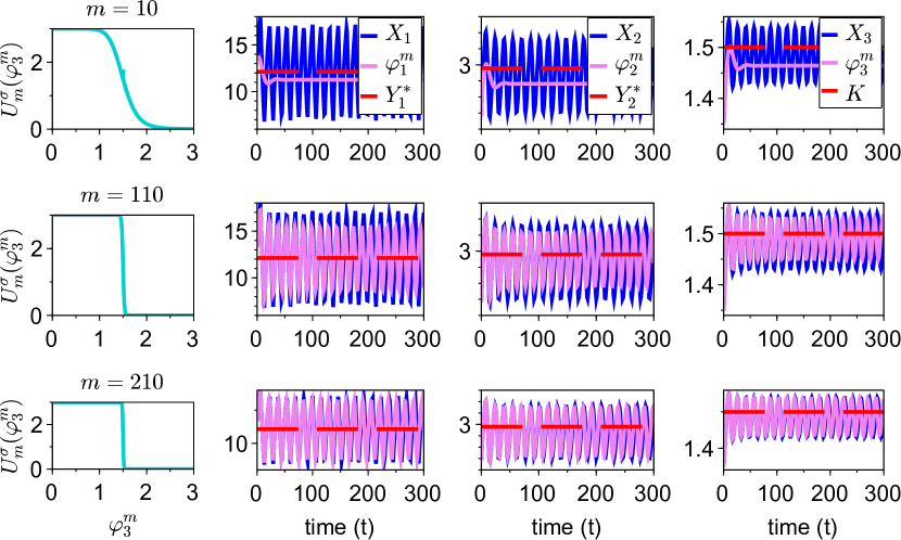
Figure 11: The switching system (21) oscillates around the sliding mode $(Y_{1}^{*},Y_{2}^{*},K)$. Functions $\varphi^{m}$ approximate $X$ as $m\to\infty$ and $\sigma\to 0$. All parameters are equal to $1$ except for $k_{1}=3$, $\nu_{n}=0.2$, $\mu=0.1$, $K=1.5$ and $\sigma=10^{-6}$. The initial conditions are $X_{1}(0)=13.34$, $X_{2}(0)=2.68$ and $X_{3}(0)=1.35$.

Figure 12: The switching system (21) converges to an equilibrium point smaller than the sliding mode $(Y_{1}^{*},Y_{2}^{*},K)$. Functions $\varphi^{m}$ approximate $X$ as $m\to\infty$ and $\sigma\to 0$. All parameters are equal to $1$ except for $k_{1}=1.6$, $\nu_{n}=0.2$, $\mu=0.1$, $K=1.5$ and $\sigma=10^{-6}$. The initial conditions are $X_{1}(0)=13.34$, $X_{2}(0)=2.68$ and $X_{3}(0)=1.35$.

Figure 13: The switching system (21) converges to the sliding mode $(Y_{1}^{*},Y_{2}^{*},K)$. Functions $\varphi^{m}$ approximate $X$ as $m\to\infty$ and $\sigma\to 0$. All parameters are equal to $1$ except for $k_{1}=\sum_{i=1}^{n-1}\mu\cdot Y_{i}^{*}+\mu\cdot K+\nu_{n}f_{n}(K)\sim 1.78$, $\nu_{n}=0.2$, $\mu=0.1$, $K=1.5$ and $\sigma=10^{-6}$. The initial conditions are $X_{1}(0)=13.34$, $X_{2}(0)=2.68$ and $X_{3}(0)=1.35$.

5.2 Piecewise linear input

In Proposition 5.4, we introduce a sequence of equations with continuous inputs (even so not everywhere differentiable). The idea is to approximate the step function defined by the switching input (2) by a sequence of piecewise linear functions of the form

$$L_{\varepsilon}\big{[}X_{n}\big{]}:=\begin{cases}k_{1}&\text{ if }X_{n}<K-\varepsilon\\ \frac{k_{1}}{2\cdot\varepsilon}(K+\varepsilon-X_{n})&\text{ if }K-\varepsilon\leq X_{n}\leq K+\varepsilon\\ 0&\text{ if }X_{n}>K+\varepsilon\\ \end{cases}$$

with $\varepsilon$ a small positive number. However, the input $L_{\varepsilon}$ above would not allow the functions of the sequence to remain constant in the sliding mode if there is $t^{*}\geq t_{0}$ such that $X_{i}(t^{*})=Y_{i}^{*}$ for every $i=1,2,\dots,n-1$ and $X_{n}(t^{*})=K$. This is a property that, according to Theorem 3.1 and Theorem 3.18, the switching systems (3) and (15) satisfy. In order to approximate this particular dynamics of the switching systems, a slightly more elaborate piecewise linear function is defined Proposition 5.4.

Proposition 5.4.

Under Assumption 1, consider the switching system

$$\frac{dX}{dt} =f(u[X_{n}],X,\mu,\nu_{n})$$

with initial conditions $X_{i}(t_{0})\geq 0$, $i=1,2,\dots,n$, $K>0$, $k_{1}>0$, $\mu\geq 0$, $\nu_{n}\geq 0$ and the input $u[X_{n}]$ defined in (2).

Suppose that there are positive values $Y_{1}^{*},Y_{2}^{*},\dots,Y_{n-1}^{*}$ such that

$$0 =f_{1}(Y_{1}^{*},Y_{2}^{*})-f_{2}(Y_{2}^{*},Y_{3}^{*})-\mu\cdot Y_{2}^{*}$$

$$0 =f_{2}(Y_{2}^{*},Y_{3}^{*})-f_{3}(Y_{3}^{*},Y_{4}^{*})-\mu\cdot Y_{3}^{*}$$

$$\vdots$$

$$0 =f_{n-1}(Y_{n-1}^{*},K)-\nu_{n}f_{n}(K)-\mu\cdot K,$$

and define

$$\alpha:=\frac{1}{k_{1}}\Big{(}\sum_{i=1}^{n-1}\mu\cdot Y_{i}^{*}+\mu\cdot K+\nu_{n}f_{n}(K)\Big{)}.$$

For every $m\in\mathbb{N}$, let $\psi^{\varepsilon}(t):=(\psi^{\varepsilon}_{1},\psi^{\varepsilon}_{2},\dots,\psi^{\varepsilon}_{n})$ be the solution for the continuous differential equation

$$\frac{d\psi^{\varepsilon}}{dt} =f\begin{pmatrix}U_{\varepsilon}\big{[}\psi^{\varepsilon}_{n}\big{]},\psi^{\varepsilon},\mu,\nu\end{pmatrix}$$

where

$$U_{\varepsilon}\big{[}\psi^{\varepsilon}_{n}\big{]}:=\begin{cases}k_{1}&\text{ if }\psi^{\varepsilon}_{n}<K-\varepsilon\\ \frac{k_{1}(\alpha-1)}{\varepsilon}(\psi^{\varepsilon}_{n}-K)+\alpha\cdot k_{1}&\text{ if }K-\varepsilon\leq\psi^{\varepsilon}_{n}<K\\ \frac{\alpha\cdot k_{1}}{\varepsilon}(K+\varepsilon-\psi^{\varepsilon}_{n})&\text{ if }K\leq\psi^{\varepsilon}_{n}<K+\varepsilon\\ 0&\text{ if }\psi^{\varepsilon}_{n}>K+\varepsilon\\ \end{cases}$$

$\varepsilon$ is a small number and the initial conditions $\psi^{\varepsilon}_{i}(t_{0})=X_{i}(t_{0})$ for all $i=1,2,\dots,n$.

Then, for a.e. $t\in[t_{0},\infty)$,

$$\lim_{\varepsilon\to 0}\psi^{\varepsilon}_{i}(t) =X_{i}(t) \forall i=1,2,\dots,n.$$

Proof 5.5.

Notice that

$$\lim_{\varepsilon\to 0}U_{\varepsilon}\big{[}\psi_{n}^{\varepsilon}\big{]}=\begin{cases}k_{1}&\text{if }\psi_{n}^{\varepsilon}<K\\ \alpha\cdot k_{1}&\text{if }\psi_{n}^{\varepsilon}=K\\ 0&\text{if }\psi_{n}^{\varepsilon}>K\end{cases}.$$

The result follows from Lemma 3 in Section 7, Chapter 2 (p. 82) of [8].

Example 5.6.

Consider the switching system (21) with reversible Michaelis-Menten kinetics introduced in Section 4. Figure 14, Figure 15 and Figure 16 illustrate the result of Proposition 5.4.

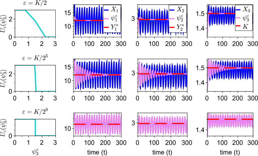
Figure 14: The switching system (21) oscillates around the sliding mode $(Y_{1}^{*},Y_{2}^{*},K)$. Functions $\psi^{\varepsilon}$ approximate $X$ as $\varepsilon\to 0$. All parameters are equal to $1$ except for $k_{1}=3$, $\nu_{n}=0.2$, $\mu=0.1$ and $K=1.5$. The initial conditions are $X_{1}(0)=13.34$, $X_{2}(0)=2.68$ and $X_{3}(0)=1.35$.

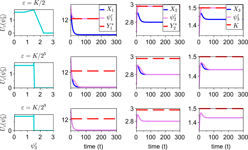
Figure 15: The switching system (21) converges to an equilibrium point smaller than the sliding mode $(Y_{1}^{*},Y_{2}^{*},K)$. Functions $\psi^{\varepsilon}$ approximate $X$ as $\varepsilon\to 0$. All parameters are equal to $1$ except for $k_{1}=1.6$, $\nu_{n}=0.2$, $\mu=0.1$ and $K=1.5$. The initial conditions are $X_{1}(0)=13.34$, $X_{2}(0)=2.68$ and $X_{3}(0)=1.35$.

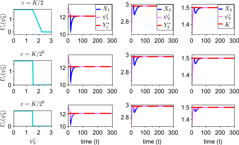
Figure 16: The switching system (21) converges to the sliding mode $(Y_{1}^{*},Y_{2}^{*},K)$. Functions $\psi^{\varepsilon}$ approximate $X$ as $\varepsilon\to 0$. All parameters are equal to $1$ except for $k_{1}=\sum_{i=1}^{n-1}\mu\cdot Y_{i}^{*}+\mu\cdot K+\nu_{n}f_{n}(K)\sim 1.78$, $\nu_{n}=0.2$, $\mu=0.1$ and $K=1.5$. The initial conditions are $X_{1}(0)=13.34$, $X_{2}(0)=2.68$ and $X_{3}(0)=1.35$.

6 Discussion and Conclusions

In this work, a model to represent allosteric regulation in a metabolic pathway is presented. In this approach, the enzymes are considered to have slow dynamics and to be therefore constant. Metabolites have faster dynamics and a ODE system based on an end-product control structure [12, 13] is studied.

Considering that allosteric processes occur very fast, the mechanism of regulation is supposed to act as a switched feedback control that is modulated according to the concentration of the end-product of the metabolic pathway. Then, a differential inclusion is defined for the discontinuous switching system and the existence and right uniqueness of an absolutely continuous solution is proved.

Moreover, the qualitative behavior of the absolutely continuous solution is analyzed and three possible trajectories are observed:

• There is a positive sliding mode and the switching system reaches it. Then the switching system stabilizes at the sliding mode.

• There is a positive sliding mode and the constant input ON is larger than a threshold defined by the sliding mode. Then the switching system oscillates around the sliding mode.

• The system with the constant input ON has a positive equilibrium point and the switching system converges uniformly and asymptotically to this, because the constant input ON is smaller than the threshold defined by the positive sliding mode (in this case the equilibrium point of the switching system is equal to or lower than the sliding mode entry by entry), or because there is no positive sliding mode.

Novel features presented in this work for the study of oscillatory behaviors are the reversibility of reactions in the metabolic pathway and the use of differential inclusions to characterize the system solutions.

The approach of Filippov [8] was necessary to study the discontinuous systems (3), (15) and (18). The existence and uniqueness of their solutions are based on that. In Section 5, we have proved that the dynamics of the discontinuous system can be approximated by continuous equations with more complex inputs than the classical sigmoid or monotone piecewise linear functions. We can then conclude that the analysis with differential inclusions has allowed to also rigorously characterize the dynamical behavior of a class of continuous feedback systems with reversible reactions and smooth or piecewise linear inputs. These results are new to our knowledge, specially concerning the oscillatory behavior.

Finally, the results obtained with this approach are potentially useful for reducing a genetic-metabolic network with slow and fast dynamics using the theory of singularly perturbed system.

Appendix A Proof of Proposition 3.6 when $\mu=0$ and $\nu_{n}>0$

Proof A.1.

Define the (Lyapunov) norm-like function

$$V(X):=\sum_{i=1}^{n}|X_{i}-X_{i}^{*}|.$$

$V$ is nonnegative and $V(X)=0$ if and only if $X_{i}=X_{i}^{*}$ for every $i=1,\dots,n$. Moreover,

$$\dot{V}= \sum_{i=1}^{n}\dot{X}_{i}\cdot sgn(X_{i}-X_{i}^{*}).$$

On the other hand, the existence of the equilibrium point guarantees

$$f_{i}(X_{i}^{*},X_{i+1}^{*}) =\mathbf{I} \forall i=1,\dots,n-1,$$

$$\nu_{n}f_{n}(X_{n}^{*}) =\mathbf{I}.$$

Then, after some algebraic computations we obtain

$$\dot{V}\leq 0$$

Therefore, $V(X)$ is decreasing. This implies that the trajectories of $X$ are bounded, since the distance to the nonnegative equilibrium point $X^{*}$ is nonincreasing.

On the other hand, the Jacobian of (5)

$$J(X)=\begin{pmatrix}-\frac{\partial f_{1}}{\partial X_{1}}&-\frac{\partial f_{1}}{\partial X_{2}}&\dots&0\\ \frac{\partial f_{1}}{\partial X_{1}}&\frac{\partial f_{1}}{\partial X_{2}}-\frac{\partial f_{2}}{\partial X_{2}}&\dots&0\\ 0&\frac{\partial f_{2}}{\partial X_{2}}&\dots&0\\ \vdots&\vdots&\ddots&\vdots\\ 0&0&\dots&-\frac{\partial f_{n-1}}{\partial X_{n}}\\ 0&0&\dots&\frac{\partial f_{n-1}}{\partial X_{n}}-\nu_{n}\frac{\partial f_{n}}{\partial X_{n}}\end{pmatrix}$$

is a compartmental matrix for every $X$ thanks to the monotonicity of the functions $f_{i}$ established Assumption 1. By Theorem 5 in [18], every orbit of (10) tends to the equilibrium set, i.e. the equilibrium $X^{*}$ is globally attractive.

Moreover, since $f_{n}$ is strictly increasing w.r.t. $X_{n}$, $\nu_{n}\frac{\partial f_{n}}{\partial X_{n}}\not=0$. Then, the Jacobian $J$ is out-flow connected. Hence, by Theorem 3 in [18], $J$ is nonsingular. By the Gershgorin Disc Theorem, a column diagonally dominant nonsingular matrix is stable. Therefore, $X^{*}$ is locally asymptotically stable. But, since $X^{*}$ is also globally attractive, we conclude that $X^{*}$ is globally asymptotically stable. Finally, since system (5) is autonomous, $X^{*}$ is globally uniformly asymptotically stable.

Appendix B Proofs of Lemmas

Proof B.1 (Proof of Lemma 3.5).

Using the monotonicity conditions set in Assumption 1 for the functions $f_{i}$, it can be proved that $\Omega_{j}$ is invariant showing that $X(t)$ points into $\Omega_{j}$ on the boundary of $\Omega_{j}$ for every $j=1,2,3,4$.

Proof B.2 (Proof of Lemma 3.9).

We will first prove that $Y_{n}^{*}<X_{n}^{*}$ by contradiction. Suppose that $X_{n}^{*}\leq Y_{n}^{*}$. We will prove by induction that $X_{i}^{*}\leq Y_{i}^{*}$ for all $i=1,2,\dots,n-1$ as well.

First, since $f_{n}$ is strictly increasing and $0\leq\mu$, this implies

$$f_{n-1}(X_{n-1}^{*},X_{n}^{*})=\nu_{n}f_{n}(X_{n}^{*})+\mu\cdot X_{n}^{*}$$

$$\leq \nu_{n}f_{n}(Y_{n}^{*})+\mu\cdot Y_{n}^{*}=f_{n-1}(Y_{n-1}^{*},Y_{n}^{*}).$$

But $f_{n-1}$ is decreasing w.r.t. to the second entry and $X_{n}^{*}\leq Y_{n}^{*}$, then

$$f_{n-1}(X_{n-1}^{*},X_{n}^{*})\leq f_{n-1}(Y_{n-1}^{*},Y_{n}^{*})\leq f_{n-1}(Y_{n-1}^{*},X_{n}^{*}).$$

Hence, since $f_{n-1}$ is strictly increasing w.r.t. to the first entry,

$$X_{n-1}^{*}\leq Y_{n-1}^{*}.$$

The induction hypothesis is that for some $m<n-1$ it is satisfied

$$X_{i}^{*} \leq Y_{i}^{*} \forall i>m.$$

We will prove that $X_{m}^{*}\leq Y_{m}^{*}$. The existence of the equilibrium points guarantees that

$$f_{m}(X_{m}^{*},X_{m+1}^{*}) =f_{m+1}(X_{m+1}^{*},X_{m+2}^{*})+\mu\cdot X_{m+1}^{*}$$

$$=\nu_{n}f_{n}(X_{n}^{*})+\sum_{i=m+1}^{n}\mu\cdot X_{i}^{*},$$

and

$$f_{m}(Y_{m}^{*},Y_{m+1}^{*}) =f_{m+1}(Y_{m+1}^{*},Y_{m+2}^{*})+\mu\cdot Y_{m+1}^{*}$$

$$=\nu_{n}f_{n}(Y_{n}^{*})+\sum_{i=m+1}^{n}\mu\cdot Y_{i}^{*},$$

But, by the induction hypothesis,

$$\nu_{n}f_{n}(X_{n}^{*})+\sum_{i=m+1}^{n}\mu\cdot X_{i}^{*}\leq\nu_{n}f_{n}(Y_{n}^{*})+\sum_{i=m+1}^{n}\mu\cdot Y_{i}^{*}.$$

Thus,

$$f_{m}(X_{m}^{*},X_{m+1}^{*}) \leq f_{m}(Y_{m}^{*},Y_{m+1}^{*})\leq f_{m}(Y_{m}^{*},X_{m+1}^{*}),$$

where the second inequality is due to hypothesis of induction $X_{m+1}^{*}\leq Y_{m+1}^{*}$ and to that $f_{m}$ is decreasing w.r.t. the second entry. Moreover, since $f_{m}$ is strictly increasing w.r.t. the first entry, we conclude that

$$X_{m}^{*}\leq Y_{m}^{*}.$$

Therefore, we have proved by induction that assuming $X_{n}^{*}\leq Y_{n}^{*}$ implies

$$X_{i}^{*} \leq Y_{i}^{*} \forall i=1,\dots,n-1.$$

But, since $f_{n}$ is strictly increasing, $0\leq\nu_{n}$ and $0\leq\mu$, this leads to conclude

$$\mathbf{I}_{1}=\sum_{i=1}^{n}\mu\cdot X_{i}^{*}+\nu_{n}f_{n}(X_{n}^{*})\leq\sum_{i=1}^{n}\mu\cdot Y_{i}^{*}+\nu_{n}f_{n}(Y_{n}^{*})=\mathbf{I}_{2},$$

which contradicts the hypothesis of that $\mathbf{I}_{2}<\mathbf{I}_{1}$. We conclude that $Y_{n}^{*}<X_{n}^{*}$. With similar arguments as above, we prove that $Y_{i}^{*}<X_{i}^{*}$ for every $i=1,2,\dots,n-1$.

Proof B.3 (Proof of Lemma 3.10).

We have that

$$f_{n-1}(X_{n-1}^{*},X_{n}^{*})=\nu_{n}f_{n}(X_{n}^{*})+\mu\cdot X_{n}^{*}.$$

Then, since $f_{n-1}$ is continuous and strictly increasing w.r.t. the first entry,

$$\nu_{n}f_{n}(X_{n}^{*})+\mu\cdot X_{n}^{*}<\lim_{X_{n-1}\to\infty}f_{n-1}(X_{n-1},X_{n}^{*}).$$

By the continuity of $f_{n}$ and $f_{n-1}$, it follows that

$$\nu_{n}f_{n}(X_{n}^{*})+\mu\cdot X_{n}^{*}=\lim_{X_{n}\to X_{n}^{*}}\nu_{n}f_{n}(X_{n})+\mu\cdot X_{n}$$

$$< \lim_{X_{n-1}\to\infty}f_{n-1}(X_{n-1},X_{n}^{*})=\lim_{X_{n}\to X_{n}^{*}}\lim_{X_{n-1}\to\infty}f_{n-1}(X_{n-1},X_{n}).$$

Then, there exists $X_{n}^{*}<X_{n}^{\prime}$ such that

$$\nu_{n}f_{n}(X_{n}^{*})+\mu\cdot X_{n}^{*}<\nu_{n}f_{n}(X_{n}^{\prime})+\mu\cdot X_{n}^{\prime}<\lim_{X_{n-1}\to\infty}f_{n-1}(X_{n-1},X_{n}^{\prime}).$$

By induction it can be proved that for any sequence $\{X_{n}^{\alpha(j)}\}_{j\in\mathbb{N}}$ such that $X_{n}^{\alpha(j)}\in(X_{n}^{*},X^{\prime}]$ for every $j=1,2,\dots$ and

$$\lim_{j\to\infty}X_{n}^{\alpha(j)}=X_{n}^{*},$$

there exists $X_{i}^{*}<X_{i}^{\alpha(j)}$, $i=1,2,\dots,n-1$, such that

$$0 =f_{1}(X_{1}^{\alpha(j)},X_{2}^{\alpha(j)})-f_{2}(X_{2}^{\alpha(j)},X_{3}^{\alpha(j)})-\mu\cdot X_{2}^{\alpha(j)}$$

$$0 =f_{2}(X_{2}^{\alpha(j)},X_{3}^{\alpha(j)})-f_{3}(X_{3}^{\alpha(j)},X_{4}^{\alpha(j)})-\mu\cdot X_{3}^{\alpha(j)}$$

$$\vdots$$

$$0 =f_{n-1}(X_{n-1}^{\alpha(j)},X_{n}^{\alpha(j)})-\nu_{n}f_{n}(X_{n}^{\alpha(j)})-\mu\cdot X_{n}^{\alpha(j)}.$$

Define

$$\mathbf{I}^{\alpha(j)}:=f_{1}(X_{1}^{\alpha(j)},X_{2}^{\alpha(j)})+\mu\cdot X_{1}^{\alpha(j)}.$$

This is satisfied, because $f_{n}$ is strictly increasing,

$$\mathbf{I}_{1} =f_{n}(X_{n}^{*})+\sum_{i=1}^{n}\mu\cdot X_{i}^{*}$$

$$<f_{n}(X_{n}^{\alpha(j)})+\sum_{i=1}^{n}\mu\cdot X_{i}^{\alpha(j)}=\mathbf{I}^{\alpha(j)},$$

and

$$\lim_{j\to\infty}\mathbf{I}^{\alpha(j)}=\mathbf{I}_{1}.$$

We conclude that, for any $0<\varepsilon$, there exists $\mathbf{I}_{1}<\mathbf{I}^{\alpha(j^{\prime})}<\mathbf{I}_{1}+\varepsilon$ such that $X_{i}^{*}<X_{i}^{\alpha(j^{\prime})}$ for all $i=1,\dots,n$ and

$$0 =\mathbf{I}^{\alpha(j^{\prime})}-f_{1}(X_{1}^{\alpha(j^{\prime})},X^{\alpha(j^{\prime})}_{2})-\mu\cdot X^{\alpha(j^{\prime})}_{1}$$

$$0 =f_{1}(X^{\alpha(j^{\prime})}_{1},X^{\alpha(j^{\prime})}_{2})-f_{2}(X^{\alpha(j^{\prime})}_{2},X^{\alpha(j^{\prime})}_{3})-\mu\cdot X^{\alpha(j^{\prime})}_{2}$$

$$\vdots$$

$$0 =f_{n-1}(X^{\alpha(j^{\prime})}_{n-1},X^{\alpha(j^{\prime})}_{n})-\nu_{n}f_{n}(X^{\alpha(j^{\prime})}_{n})-\mu\cdot X^{\alpha(j^{\prime})}_{n}.$$

Proof B.4 (Proof of Lemma 3.8).

Define

$$Z_{i}(t) :=X_{i}(t)-Y_{i}(t) t\geq t_{0},\forall i=1,2,\dots,n.$$

The first conclusion of the Lemma follows from the fact that the sets

$$\mathbb{R}^{n}_{+}:=\underset{n\text{-times}}{[0,\infty)\times[0,\infty)\times\dots\times[0,\infty)},$$

$$int(\mathbb{R}^{n}_{+}):=\underset{n\text{-times}}{(0,\infty)\times(0,\infty)\times\dots\times(0,\infty)},$$

are invariant under the flow $Z(t)$ if $\mathbf{I}_{2}<\mathbf{I}_{1}$.

On the other hand, if $\mathbf{I}_{1}=\mathbf{I}_{2}$ and $Y_{i}(t_{0})<X_{i}(t_{0})$ for every $i=1,2,\dots,n$, then, by the continuity of $Z$, there is $\varepsilon>0$ such that for all $i=1,2,\dots,n$

$$0<Z_{i}(t) :=X_{i}(t)-Y_{i}(t) t_{0}<t<t_{0}+\varepsilon.$$

With similar arguments as above, it can be proved that $\mathbb{R}^{n}_{+}$ is positively invariant under the flow of $Z$.

Proof B.5 (Proof of Lemma 3.13).

The proof can be done by induction over $m$, i.e., first proving the Lemma when $m=n-1$, assuming the Lemma as the induction hypothesis for some $m+1$ and proving it for the case $m$.

Proof B.6 (Proof of Lemma 3.14).

By hypothesis,

$$sgn(\dot{\widetilde{X}}_{n}(t_{0})) =sgn(\dot{Z}_{n}(t_{0})).$$

Suppose that $sgn(\dot{\widetilde{X}}_{n}(t_{0}))<0$. Then, by the continuity of $\dot{\widetilde{X}}_{n}$ and $\dot{Z}_{n}$, there exist $\varepsilon_{1}$ and $\varepsilon_{2}$ such that

$$sgn(\dot{\widetilde{X}}_{n}(t)) <0 \forall t\in(t_{0},t_{0}+\varepsilon_{1}),$$

$$sgn(\dot{Z}_{n}(t)) <0 \forall t\in(t_{0},t_{0}+\varepsilon_{2}).$$

Hence, if $\varepsilon:=\min\{\varepsilon_{1},\varepsilon_{2}\}$,

$$sgn(\dot{\widetilde{X}}_{n}(t)) =sgn(\dot{Z}_{n}(t))<0 \forall t\in(t_{0},t_{0}+\varepsilon).$$

Analogously, if $0<sgn(\dot{\widetilde{X}}_{n}(t_{0}))$, by the continuity of $\dot{\widetilde{X}}_{n}$ and $\dot{Z}_{n}$, there exist $\varepsilon_{1}$ and $\varepsilon_{2}$ such that

$$0< sgn(\dot{\widetilde{X}}_{n}(t)) \forall t\in(t_{0},t_{0}+\varepsilon_{1}),$$

$$0< sgn(\dot{Z}_{n}(t)) \forall t\in(t_{0},t_{0}+\varepsilon_{2}).$$

Hence, if $\varepsilon:=\min\{\varepsilon_{1},\varepsilon_{2}\}$,

$$0<sgn(\dot{\widetilde{X}}_{n}(t)) =sgn(\dot{Z}_{n}(t)) \forall t\in(t_{0},t_{0}+\varepsilon).$$

Assume that $sgn(\dot{\widetilde{X}}_{n}(t_{0}))=0$. If there exist $\varepsilon_{1}$ and $\varepsilon_{2}$ such that

$$sgn(\dot{\widetilde{X}}_{n}(t))<0 \forall t\in(t_{0},t_{0}+\varepsilon_{1}),$$

$$0<sgn(\dot{Z}_{n}(t)) \forall t\in(t_{0},t_{0}+\varepsilon_{2}),$$

then,

$$\dot{\widetilde{X}}_{n}(t)<\dot{\widetilde{X}}_{n}(t_{0})<\dot{Z}_{n}(t) \forall t\in(t_{0},t_{0}+\varepsilon),$$

where $\varepsilon:=\min\{\varepsilon_{1},\varepsilon_{2}\}$. But the inequality above contradicts Lemma 3.8, since $0<k_{1}$.

We cannot suppose there exist $\varepsilon_{1}$ and $\varepsilon_{2}$ such that

$$sgn(\dot{\widetilde{X}}_{n}(t)) =0 \forall t\in[t_{0},t_{0}+\varepsilon_{1})$$ or

$$sgn(\dot{Z}_{n}(t)) =0 \forall t\in[t_{0},t_{0}+\varepsilon_{2}),$$

because this leads to conclude that the systems are at equilibrium in $[t_{0},t_{0}+\varepsilon)$.

But this contradicts the hypothesis, as it was assumed

$$\dot{Z}_{m}(t_{0}) =\dot{\widetilde{X}}_{m}(t_{0})\not=0 \text{for some }m\in\{1,2,\dots,n\}.$$

Now suppose $sgn(\dot{\widetilde{X}}_{n}(t_{0}))=0$ and there exist $\varepsilon_{1}$ and $\varepsilon_{2}$ such that

$$0<sgn(\dot{\widetilde{X}}_{n}(t)) \forall t\in(t_{0},t_{0}+\varepsilon_{1}),$$

$$sgn(\dot{Z}_{n}(t))<0 \forall t\in(t_{0},t_{0}+\varepsilon_{2}).$$

(One option is to say that this contradicts Proposition 3.15 (existence of solution theorem of Filippov, Theorem 1, p. 77 in [8]), another option is as follows).

According to the hypothesis, $\dot{\widetilde{X}}_{m}(t_{0})=\dot{Z}_{m}(t_{0})\not=0$ for some $1<m<n$. Without loss of generality, assume that $\dot{\widetilde{X}}_{i}(t_{0})=\dot{Z}_{i}(t_{0})=0$ for every $m<i$ Hence, let us assume that there is $0<\varepsilon<\min\{\varepsilon_{1},\varepsilon_{2}\}$ such that

$$0 <sgn(\dot{\widetilde{X}}_{m}(t))=sgn(\dot{Z}_{m}(t)) \forall t\in[t_{0},t_{0}+\varepsilon).$$

This implies, according to Lemma 3.13,

$$0 <sgn(\dot{\widetilde{X}}_{i}(t))=sgn(\dot{Z}_{i}(t)) \forall t\in(t_{0},t_{0}+\varepsilon),\forall i>m,$$

that contradicts the supposition

$$sgn(\dot{Z}_{n}(t))<0 \forall t\in(t_{0},t_{0}+\varepsilon_{2}).$$

Analogously, by Lemma 3.13, assuming

$$sgn(\dot{\widetilde{X}}_{m}(t))=sgn(\dot{Z}_{m}(t)) <0 \forall t\in[t_{0},t_{0}+\varepsilon),$$

implies for all $i>m$

$$sgn(\dot{\widetilde{X}}_{i}(t))=sgn(\dot{Z}_{i}(t))<0 \forall t\in(t_{0},t_{0}+\varepsilon),$$

that contradicts the supposition

$$0<sgn(\dot{\widetilde{X}}_{n}(t)) \forall t\in(t_{0},t_{0}+\varepsilon_{1}).$$

We conclude that is false that $sgn(\dot{\widetilde{X}}_{n}(t_{0}))=0$ and there exist $\varepsilon_{1}$ and $\varepsilon_{2}$ such that

$$0<sgn(\dot{\widetilde{X}}_{n}(t)) \forall t\in(t_{0},t_{0}+\varepsilon_{1}),$$

$$sgn(\dot{Z}_{n}(t))<0 \forall t\in(t_{0},t_{0}+\varepsilon_{2}).$$

Proof B.7 (Proof of Lemma 3.20).

Consider any $X_{n}^{\prime}\in(0,X_{n}^{*})$. According to Assumption 1,

$$f_{n-1}(0,X_{n}^{\prime})\leq 0<\nu_{n}f_{n}(X_{n}^{\prime})+\mu\cdot X_{n}^{\prime}<f_{n-1}(X_{n-1}^{*},X_{n}^{\prime})$$

Then, since $f_{n-1}$ is strictly increasing w.r.t. the first entry, there exists an unique $X_{n-1}^{\prime}\in(0,X_{n-1}^{*})$ such that

$$f_{n-1}(X_{n-1}^{\prime},X_{n}^{\prime})=\nu_{n}f_{n}(X_{n}^{\prime})+\mu\cdot X_{n}^{\prime}.$$

The proof follows by induction.

Proof B.8 (Proof of Lemma 3.21).

The trivial case where the hybrid system $X$ never switches follows from Lemma 3.8.

Now suppose that the hybrid system switches. By the continuity of $X_{n}$, there exists a countable $\mathbf{N}:=\{0,1,2,\dots,k\}\subset\mathbb{N}$ and values $\{t_{j}\}_{j\in\mathbb{N}}\subset\mathbb{R}^{+}$, with $t_{j}<t_{j+1}$ for every $j\in\mathbb{N}$, such that the switching system is under a single regime in any interval $(t_{j},t_{j+1})$ for every $j\in\mathbb{N}$ (i.e. $X_{n}(t)\leq K$ for all $t\in(t_{j},t_{j+1})$ or $K<X_{n}(t)$ for all $t\in(t_{j},t_{j+1})$).

It can be proved by induction, using Lemma 3.8, that for every $j\in\mathbb{N}$,

$$X_{i}(t) \leq\widetilde{X}_{i}(t) \forall t\in(t_{j},t_{j+1}),\forall i=1,2,\dots,n.$$

Furthermore, by continuity of $X_{i}$ and $\widetilde{X}_{i}$,

$$X_{i}(t_{j}) \leq\widetilde{X}_{i}(t_{j}) \forall i=1,2,\dots,n, \forall j\in\mathbb{N}.$$

Appendix C Comparison with a piecewise linear model

Here we present an example for comparison with the approach of piecewise linear models first proposed by Glass and Pasternack in [51]. The following piecewise linear model is based on the model proposed by Poignard et al. in [49]:

(29) $$\frac{dX_{1,Bool}}{dt} :=k_{1}\cdot(1-s^{+}(X_{3,Bool},K))-\mu\cdot X_{1,Bool}$$

$$\frac{dX_{2,Bool}}{dt} :=k_{2}\cdot s^{+}(X_{1,Bool},Y_{1}^{*})-\mu\cdot X_{2,Bool}$$

$$\frac{dX_{3,Bool}}{dt} :=k_{3}\cdot s^{+}(X_{2,Bool},Y_{2}^{*})-\mu\cdot X_{3,Bool},$$

where the boolean functions are defined as

$$s^{+}(X_{i,Bool},Y_{i}^{*}) :=\begin{cases}1&\text{if }X_{i,Bool}>Y_{i}^{*}\\ 0&\text{if }X_{i,Bool}<Y_{i}^{*}\end{cases} i=1,2,$$

$$s^{+}(X_{3,Bool},K) :=\begin{cases}1&\text{if }X_{3,Bool}>K\\ 0&\text{if }X_{3,Bool}<K.\end{cases}$$

To compare the piecewise model (29) with a hybrid model as proposed in this article consider

(30) $$\frac{dX_{1}}{dt} :=u[X_{3}]-k_{2}\cdot X_{1}-\mu\cdot X_{1}$$

$$\frac{dX_{2}}{dt} :=k_{2}\cdot X_{1}-k_{3}\cdot X_{2}-\mu\cdot X_{2}$$

$$\frac{dX_{3}}{dt} :=k_{3}\cdot X_{2}-\mu\cdot X_{3},$$

where $u[X_{3}]$ is defined as in (2). Notice that, in contrast to (29), mass-action kinetics are considered in (30). This property of the class of models studied in this work has been recurrently used in the demonstration of our results. In Figure 17 are depicted numerical solutions for systems (29) and (30). They both exhibit oscillations crossing the sliding mode $(Y_{1}^{*},Y_{2}^{*},K)$, but with different magnitude and amplitude of oscillations.

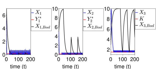
Figure 17: Numerical solution of (29) and (30). All parameters are equal to 1 except for $K=1.5$ and $\mu=0.1$. The vector $(Y_{1}^{*},Y_{2}^{*},K)$ corresponds to the sliding mode equilibrium point of (30) (see Theorem 3.1). The solutions of (29) and (30) were computed in Scilab using the Runge-Kutta and ode functions, respectively. Both models (29) and (30) exhibit oscillations crossing the sliding mode $(Y_{1}^{*},Y_{2}^{*},K)$, but with different magnitude and amplitude of oscillations.

References

• [1] D. Allwright, A global stability criterion for simple control loops, Journal of Mathematical Biology, 4 (1977), pp. 363–373.
• [2] J. Anderson, Y.-C. Chang, and A. Papachristodoulou, Model decomposition and reduction tools for large-scale networks in systems biology, Automatica, 47 (2011), pp. 1165–1174.
• [3] M. Arcak and E. D. Sontag, Diagonal stability of a class of cyclic systems and its connection with the secant criterion, Automatica, 42 (2006), pp. 1531–1537.
• [4] V. Baldazzi, D. Ropers, J. Geiselmann, D. Kahn, and H. de Jong, Importance of metabolic coupling for the dynamics of gene expression following a diauxic shift in escherichia coli, Journal of theoretical biology, 295 (2012), pp. 100–115.
• [5] M. Chaves and D. A. Oyarzún, Dynamics of complex feedback architectures in metabolic pathways, Automatica, 99 (2019), pp. 323–332.
• [6] H. El Samad, M. Khammash, L. Petzold, and D. Gillespie, Stochastic modelling of gene regulatory networks, International Journal of Robust and Nonlinear Control: IFAC-Affiliated Journal, 15 (2005), pp. 691–711.
• [7] N. Fenichel, Geometric singular perturbation theory for ordinary differential equations, Journal of differential equations, 31 (1979), pp. 53–98.
• [8] A. Filippov, Differential equations with discontinuous righthand sides, Springer Science & Business Media, 1988.
• [9] E. Fung, W. W. Wong, J. K. Suen, T. Bulter, S.-g. Lee, and J. C. Liao, A synthetic gene–metabolic oscillator, Nature, 435 (2005), pp. 118–122.
• [10] Z. P. Gerdtzen, P. Daoutidis, and W.-S. Hu, Non-linear reduction for kinetic models of metabolic reaction networks, Metabolic engineering, 6 (2004), pp. 140–154.
• [11] A. Goeke and S. Walcher, A constructive approach to quasi-steady state reductions, Journal of mathematical chemistry, 52 (2014), pp. 2596–2626.
• [12] A. Goelzer, F. B. Brikci, I. Martin-Verstraete, P. Noirot, P. Bessières, S. Aymerich, and V. Fromion, Reconstruction and analysis of the genetic and metabolic regulatory networks of the central metabolism of bacillus subtilis, BMC systems biology, 2 (2008), p. 20.
• [13] A. Goelzer and V. Fromion, Towards the modular decomposition of the metabolic network, in A Systems Theoretic Approach to Systems and Synthetic Biology I: Models and System Characterizations, Springer, 2014, pp. 121–152.
• [14] A. Goelzer, V. Fromion, and G. Scorletti, Cell design in bacteria as a convex optimization problem, Automatica, 47 (2011), pp. 1210–1218.
• [15] R. Heinrich and T. Rapoport, Mathematical analysis of multienzyme systems. II. steady state and transient control, Biosystems, 7 (1975), pp. 130–136.
• [16] F. Horn and R. Jackson, General mass action kinetics, Archive for rational mechanics and analysis, 47 (1972), pp. 81–116.
• [17] F. Jacob and J. Monod, Genetic regulatory mechanisms in the synthesis of proteins, Journal of molecular biology, 3 (1961), pp. 318–356.
• [18] J. A. Jacquez and C. P. Simon, Qualitative theory of compartmental systems, Siam Review, 35 (1993), pp. 43–79.
• [19] H. Kacser and J. A. Burns, The control of flux, Symposia of the Society for Experimental Biology, 27 (1973).
• [20] H. Khalil, Nonlinear systems, Prentice Hall, New Jersey, third edition, 2002.
• [21] J. K. Kim, K. Josić, and M. R. Bennett, The validity of quasi-steady-state approximations in discrete stochastic simulations, Biophysical journal, 107 (2014), pp. 783–793.
• [22] P. Kokotović, H. K. Khalil, and J. O’reilly, Singular perturbation methods in control: analysis and design, SIAM, 1999.
• [23] J. Kuntz, D. Oyarzún, and G.-B. Stan, Model reduction of genetic-metabolic networks via time scale separation, in A systems theoretic approach to systems and synthetic biology I: models and system characterizations, Springer, 2014, pp. 181–210.
• [24] J. A. Lerman, D. R. Hyduke, H. Latif, V. A. Portnoy, N. E. Lewis, J. D. Orth, A. C. Schrimpe-Rutledge, R. D. Smith, J. N. Adkins, K. Zengler, et al., In silico method for modelling metabolism and gene product expression at genome scale, Nature communications, 3 (2012), pp. 1–10.
• [25] L. Liu and A. Bockmayr, Regulatory dynamic enzyme-cost flux balance analysis: A unifying framework for constraint-based modeling, Journal of Theoretical Biology, (2020), p. 110317.
• [26] C. Lopez-Zazueta, O. Bernard, and J.-L. Gouzé, Analytical reduction of nonlinear metabolic networks accounting for dynamics in enzymatic reactions, Complexity, 2018 (2018).
• [27] C. Lopez-Zazueta, O. Bernard, and J.-L. Gouzé, Dynamical reduction of linearized metabolic networks through quasi steady state approximation, AIChE Journal, 65 (2019), pp. 18–31.
• [28] A. Mees and P. Rapp, Periodic metabolic systems: oscillations in multiple-loop negative feedback biochemical control networks, Journal of Mathematical Biology, 5 (1978), pp. 99–114.
• [29] N. Meslem and V. Fromion, Lyapunov function for irreversible linear metabolic pathways with allosteric and genetic regulation, in 2011 50th IEEE Conference on Decision and Control and European Control Conference, IEEE, 2011, pp. 5182–5187.
• [30] N. Meslem, V. Fromion, A. Goelzer, and L. Tournier, Stability analysis for bacterial linear metabolic pathways with monotone control system theory, in 7. International Conference on Informatics in Control, Automation and Robotics, Springer-Verlag, 2010.
• [31] I. Ndiaye and J.-L. Gouzé, Global stability of reversible enzymatic metabolic chains, Acta biotheoretica, 61 (2013), pp. 41–57.
• [32] Y. Orlov, Discontinuous systems: Lyapunov analysis and robust synthesis under uncertainty conditions, Springer Science & Business Media, 2009.
• [33] J. D. Orth, I. Thiele, and B. Ø. Palsson, What is flux balance analysis?, Nature biotechnology, 28 (2010), pp. 245–248.
• [34] D. A. Oyarzún, M. Chaves, and M. Hoff-Hoffmeyer-Zlotnik, Multistability and oscillations in genetic control of metabolism, Journal of theoretical biology, 295 (2012), pp. 139–153.
• [35] O. Radulescu, A. N. Gorban, A. Zinovyev, and A. Lilienbaum, Robust simplifications of multiscale biochemical networks, BMC systems biology, 2 (2008), p. 86.
• [36] C. V. Rao and A. P. Arkin, Stochastic chemical kinetics and the quasi-steady-state assumption: Application to the gillespie algorithm, The Journal of chemical physics, 118 (2003), pp. 4999–5010.
• [37] T. A. Rapoport, R. Heinrich, G. Jacobasch, and S. Rapoport, A linear steady-state treatment of enzymatic chains: A mathematical model of glycolysis of human erythrocytes, European Journal of Biochemistry, 42 (1974), pp. 107–120.
• [38] C. Reder, Metabolic control theory: a structural approach, Journal of theoretical biology, 135 (1988), pp. 175–201.
• [39] M. A. Savageau, Biochemical systems analysis: I. some mathematical properties of the rate law for the component enzymatic reactions, Journal of theoretical biology, 25 (1969), pp. 365–369.
• [40] A. Tikhonov, A. B. Vasil’eva, and A. G. Sveshnikov, Differential Equations, Springer-Verlag, Berlin, 1985.
• [41] J. J. Tyson and H. G. Othmer, The dynamics of feedback control circuits in biochemical pathways, Progress in theoretical biology, 5 (1978), pp. 1–62.
• [42] A. Varma and B. O. Palsson, Metabolic flux balancing: basic concepts, scientific and practical use, Bio/technology, 12 (1994), pp. 994–998.
• [43] F. Verhulst, Singular perturbation methods for slow–fast dynamics, Nonlinear Dynamics, 50 (2007), pp. 747–753.
• [44] E. O. Voit, H. A. Martens, and S. W. Omholt, 150 years of the mass action law, PLoS Comput Biol, 11 (2015), p. e1004012.
• [45] S. Waldherr, D. A. Oyarzún, and A. Bockmayr, Dynamic optimization of metabolic networks coupled with gene expression, Journal of theoretical biology, 365 (2015), pp. 469–485.
• [46] L. Wang, P. De Leenheer, and E. D. Sontag, Conditions for global stability of monotone tridiagonal systems with negative feedback, Systems & control letters, 59 (2010), pp. 130–138.
• [47] Hastings, Stuart and Tyson, John and Webster, Dallas, Existence of periodic solutions for negative feedback cellular control systems, Journal of Differential Equations, 25, 1, 39–64, 1977, Academic Press
• [48] Mallet-Paret, John and Smith, Hal, The Poincaré-Bendixson theorem for monotone cyclic feedback systems, Journal of Dynamics and Differential Equations, 2, 4, 367–421, 1990, Springer New York
• [49] Poignard, Camille and Chaves, Madalena and Gouzé, Jean-Luc, Periodic oscillations for nonmonotonic smooth negative feedback circuits, SIAM Journal on Applied Dynamical Systems, 15, 1, 257–286, 2016, SIAM
• [50] Poignard, Camille and Chaves, Madalena and Gouzé, Jean-Luc, A stability result for periodic solutions of nonmonotonic smooth negative feedback systems, SIAM Journal on Applied Dynamical Systems, 17, 2, 1091–1116, 2018, SIAM
• [51] Glass, Leon and Pasternack, Joel S, Stable oscillations in mathematical models of biological control systems, Journal of Mathematical Biology, 6, 3, 207–223, 1978, Springer
• [52] Farcot, Etienne and Gouzé, Jean-Luc, Periodic solutions of piecewise affine gene network models with non uniform decay rates: the case of a negative feedback loop, Acta Biotheoretica, 57, 4, 429–455, 2009, Springer
• [53] Quee, G and Edwards, R, Ramp approximations of sigmoid control functions in gene networks, Physica D: Nonlinear Phenomena, 418, 132840, 2021, Elsevier
• [54] Farcot, Etienne and Gouzé, Jean-Luc, Limit cycles in piecewise-affine gene network models with multiple interaction loops, International Journal of Control, 41, 1, 119–130, 2010, Taylor & Francis
• [55] Casey, Richard and Jong, Hidde de and Gouzé, Jean-Luc, Piecewise-linear models of genetic regulatory networks: equilibria and their stability, Journal of mathematical biology, 52, 1, 27–56, 2006, Springer
• [56] Duncan, William and Gedeon, Tomas and Kokubu, Hiroshi and Mischaikow, Konstantin and Oka, Hiroe, Equilibria and their stability in networks with steep sigmoidal nonlinearities, SIAM Journal on Applied Dynamical Systems, 20, 4, 2108–2141, 2021, SIAM
• [57] Plahte, Erik and Mestl, Thomas and Omholt, Stig W, Global analysis of steady points for systems of differential equations with sigmoid interactions, Dynamics and Stability of Systems, 9, 4, 275–291, 1994, Taylor & Francis
• [58] Mestl, Thomas and Plahte, Erik and Omholt, Stig W, A mathematical framework for describing and analysing gene regulatory networks, Journal of theoretical Biology, 176, 2, 291–300, 1995, Elsevier