Lorentz-covariant kinetic theory for massive spin-1/2 particles

Abstract

We construct a matrix-valued spin-dependent distribution function (MVSD) for massive spin-1/2 fermions and study its properties under Lorentz transformations. Such transformations result in a Wigner rotation in spin space and in a nontrivial matrix-valued shift in space-time, which corresponds to the side jump in the massless case. We express the vector and axial-vector components of the Wigner function in terms of the MVSD and show that they transform in a Lorentz-covariant manner. We then construct a manifestly Lorentz-covariant Boltzmann equation which contains a nonlocal collision term encoding spin-orbit coupling. Finally, we obtain the spin-dependent distribution function in local equilibrium by demanding detailed balance.

Introduction. —

In noncentral heavy-ion collisions, a part of the large orbital angular momentum (OAM) of the system is converted into polarization of final-state hadrons Liang and Wang (2005a, b); Voloshin (2004). The polarization of $\Lambda$ and $\bar{\Lambda}$ hyperons along the direction of the global OAM has been experimentally measured by the STAR collaboration Adamczyk et al. (2017); Adam et al. (2018) and agrees well with theoretical calculations Becattini et al. (2013); Karpenko and Becattini (2017); Wei et al. (2019). However, the dependence on azimuthal angle of the longitudinal polarization of $\Lambda$’s Adam et al. (2019) shows the opposite sign as in theoretical frameworks which reproduce the global polarization. Various efforts Florkowski et al. (2019a); Sun and Ko (2019); Florkowski et al. (2019b); Becattini et al. (2019a); Xia et al. (2019); Wu et al. (2019); Liu et al. (2020) have been made to resolve this so-called “sign problem of the longitudinal polarization”, but a fully convincing explanation does not yet exist. It was recently proposed Becattini et al. (2021a); Liu and Yin (2021); Fu et al. (2021); Becattini et al. (2021b) that previous calculations had missed a shear-induced contribution to the polarization at freeze-out, which has the potential to solve this problem, but so far results including this term appear to be sensitive to the equation of state and other parameters of the calculation Yi et al. (2021).

Therefore, from both the theoretical and the experimental perspective, a consistent way to describe the dynamics of spin in heavy-ion collisions is urgently needed. Recently, a lot of activity was devoted to deriving kinetic theory for massive particles with spin Zhang et al. (2019); Li and Yee (2019); Liu and Huang (2020); Yang et al. (2020); Weickgenannt et al. (2020); Li (2021); Manuel and Torres-Rincon (2021); Weickgenannt et al. (2021); Sheng et al. (2021); Lin (2021) and spin hydrodynamics Florkowski et al. (2018a, b); Montenegro et al. (2017); Florkowski et al. (2019c, 2018c); Becattini et al. (2019b); Hattori et al. (2019a); Bhadury et al. (2021); Montenegro and Torrieri (2020); Li et al. (2021). The dynamics of massless particles is described by Chiral Kinetic Theory (CKT), first proposed in Refs. Son and Yamamoto (2012); Stephanov and Yin (2012); Chen et al. (2013). The helicity, defined as the product of momentum and spin, is Lorentz invariant. However, both the momentum and the spin of a particle will change under a Lorentz boost, in order to preserve the helicity. Conservation of total angular momentum then requires that the OAM of the particle also changes. This in general implies that the particle’s position will undergo a nontrivial shift, which is called the side-jump effect Chen et al. (2014a, 2015); Hidaka et al. (2017). On the other hand, it has been realized that the collisionless kinetic theory for massive particles can be smoothly connected to CKT, if one properly defines the reference frame Sheng et al. (2020) or if one directly replaces the spin vector by the momentum vector Gao and Liang (2019); Weickgenannt et al. (2019); Wang et al. (2019); Hattori et al. (2019b). Such a connection exists because Wigner’s little group for massless particles can be obtained from that for massive particles by taking the infinite-momentum limit and the massless limit at the same time, indicating that spin for massive particles reduces to helicity in this limit Wigner (1939); Kim and Wigner (1987, 1990). Then, one naturally expects that the massless limit for the collision term as well as for the equilibrium distribution agrees with the result from CKT Chen et al. (2015); Hidaka et al. (2017, 2018). In order to confirm this expectation, we need to discard any reference to the rest frame of a massive particle, as such a frame does not exist for massless particles. Instead, we need to consider a Lorentz boost between two arbitrary reference frames.

In this work, we derive a matrix-valued spin-dependent distribution function (MVSD) and show that its Lorentz-transformation properties are highly nontrivial: in addition to a Wigner rotation in spin space, the MVSD undergoes a matrix-valued shift in space-time, which is similar to the side-jump effect for massless particles. Using this MVSD, we then construct a Lorentz-covariant Boltzmann equation with a nonlocal collision term, which forms the theoretical foundation for a consistent description of the dynamics of massive spin-1/2 particles in heavy-ion collisions. It constitutes a well-founded theory for numerical simulations of spin polarization and thus may potentially contribute to solving the sign problem of the longitudinal polarization.

Matrix-valued spin-dependent distribution function. —

We define a plane-wave state as

$$|\mathbf{p},s\rangle\equiv a_{\mathbf{p},s}^{\dagger}|0\rangle\;,$$ (1)

where $a_{\mathbf{p},s}^{\dagger}$ is the creation operator for a particle with momentum $\mathbf{p}$ and spin $s$, with the corresponding annihiliation operator being $a_{\mathbf{p},s}$, fulfilling the anticommutation relation $\left\{a_{\mathbf{p},s}^{\dagger},a_{\mathbf{p}^{\prime},s^{\prime}}\right\}=2E_{\mathbf{p}}(2\pi\hbar)^{3}\delta^{(3)}(\mathbf{p}-\mathbf{p}^{\prime})\delta_{ss^{\prime}}$, with the mass-shell energy $E_{\bf p}\equiv\sqrt{{\bf p}^{2}+m^{2}}$. The density matrix is defined as

$$\rho\equiv\sum_{rs}\int Dp_{1}\int Dp_{2}\,\tilde{f}_{rs}(\mathbf{p}_{1},\mathbf{p}_{2})\left|\mathbf{p}_{1},r\right\rangle\left\langle\mathbf{p}_{2},s\right|\;,$$ (2)

where the invariant momentum-integration measure is defined as $Dp\equiv d^{3}{\bf p}/\left[(2\pi\hbar)^{3}2E_{{\bf p}}\right]$. The MVSD in momentum space is given as $\tilde{f}_{rs}(\mathbf{p}_{1},\mathbf{p}_{2})=\left\langle a_{\mathbf{p}_{2},s}^{\dagger}a_{\mathbf{p}_{1},r}\right\rangle$, where $\langle\mathcal{O}\rangle\equiv\mathrm{Tr}(\rho\,\mathcal{O})$ denotes the expectation value of the operator $\mathcal{O}$ in the ensemble characterized by the density matrix (2). We define the MVSD in phase space by taking the Fourier transform with respect to the relative momentum $q^{\mu}\equiv p_{1}^{\mu}-p_{2}^{\mu}$,

$$f_{rs}(x,p)\equiv\int\frac{d^{4}q}{2(2\pi\hbar)^{3}}\exp\left(-\frac{i}{\hbar}q\cdot x\right)\delta(p\cdot q)\tilde{f}_{rs}(\mathbf{p}_{1},\mathbf{p}_{2})\;,$$ (3)

where $p^{\mu}\equiv(p_{1}^{\mu}+p_{2}^{\mu})/2$ is the average momentum. The MVSD (3) is a generalization of the classical distribution function to the case of quantum particles with spin 1/2, which satisfies $f_{rs}^{\ast}=f_{sr}$, indicating that $f_{rs}(x,p)$ is a Hermitian matrix. We note that $p_{1}^{\mu}$ and $p_{2}^{\mu}$ are restricted to the mass-shell $p_{1}^{2}=p_{2}^{2}=m^{2}$, leading to the constraint $p\cdot q=0$. The MVSD has previously been used to derive the equilibrium form of the polarization (Becattini and Tinti, 2010; Becattini et al., 2013). In this work, we will derive the Boltzmann equation for the MVSD that describes its dynamical evolution in a nonequilibrium system.

For a system of weakly interacting particles, one expects that $\tilde{f}_{rs}(\mathbf{p}_{1},\mathbf{p}_{2})$ has nonvanishing values only when $|{\bf p}_{1}-{\bf p}_{2}|=|\mathbf{q}|\ll|\mathbf{p}|=|{\bf p}_{1}+{\bf p}_{2}|$. As a consequence, the gradient of the MVSD (3) satisfies $\hbar\left|\boldsymbol{\nabla}_{{\bf x}}f_{rs}(x,p)\right|\ll\left|{\bf p}f_{rs}(x,p)\right|$, ensuring the validity of the $\hbar$ expansion, which we will employ in the following.

Wigner function. —

We now relate the MVSD (3) to the Wigner function Heinz (1983); Vasak et al. (1987)

$$W(x,p)=\int\frac{d^{4}y}{(2\pi\hbar)^{4}}e^{-ip\cdot y/\hbar}\left\langle\bar{\psi}\left(x+\frac{y}{2}\right)\otimes\psi\left(x-\frac{y}{2}\right)\right\rangle,$$ (4)

where $\otimes$ denotes the Kronecker product. Let us consider the collisionless case, i.e., we assume that the Dirac-field operators in Eq. (4) fulfill the non-interacting Dirac equation Itzykson and Zuber (1980). Inserting these operators into the definition (4), performing a gradient expansion, and keeping terms of first order in $\hbar$ we arrive at

$$W(x,p) \equiv\frac{1}{(2\pi)^{3}}\theta(p^{0})\delta(p^{2}-m^{2})$$

$$\!\!\!\!\!\!\!\!\!\!\!\!\!\!\!\!\!\!\times\sum_{rs}\left[\bar{u}_{s}(\mathbf{p})\otimes u_{r}(\mathbf{p})+i\hbar\,\boldsymbol{\mathcal{U}}_{sr}({\bf p})\cdot\boldsymbol{\nabla}_{\mathbf{x}}\right]f_{rs}(x,p)\;.$$ (5)

The momentum in Eq. (5) is restricted to the mass-shell $p^{2}=m^{2}$, while off-shell corrections arise at second order in $\hbar$. The matrix-valued Berry connection for Dirac fermions is defined as Chen et al. (2014b); Sheng et al. (2020)

$$\boldsymbol{\mathcal{U}}_{sr}({\bf p})\equiv\frac{1}{2}\!\left\{\vphantom{\frac{}{}}\!\left[\boldsymbol{\nabla}_{\mathbf{p}}\bar{u}_{s}(\mathbf{p})\right]\otimes u_{r}(\mathbf{p})-\bar{u}_{s}(\mathbf{p})\otimes\left[\boldsymbol{\nabla}_{\mathbf{p}}u_{r}(\mathbf{p})\right]\!\right\},$$ (6)

which is a $2\times 2$ matrix in spin space and a $4\times 4$ matrix in Dirac space.

We further decompose the Wigner function in terms of the generators of the Clifford algebra,

$$W=\frac{1}{4}\left(\mathcal{F}+i\gamma^{5}\mathcal{P}+\gamma^{\mu}\mathcal{V}_{\mu}+\gamma^{5}\gamma^{\mu}\mathcal{A}_{\mu}+\frac{1}{2}\sigma^{\mu\nu}\mathcal{S}_{\mu\nu}\right)\;,$$ (7)

where $\sigma^{\mu\nu}\equiv\frac{i}{2}[\gamma^{\mu},\gamma^{\nu}]$. The vector component $\mathcal{V}^{\mu}$ has a clear physical meaning: it is the current density in phase space Vasak et al. (1987). Its zeroth component, $\mathcal{V}^{0}\equiv\text{Tr}(\gamma^{0}W)$, where “Tr” denotes the trace in Dirac space, is given by

$$\mathcal{V}^{0}=\frac{2}{(2\pi\hbar)^{3}}\theta(p^{0})\delta(p^{2}-m^{2})E_{{\bf p}}\,\text{tr}\left[F(x,p)\right]\;,$$ (8)

where “tr” denotes the trace in spin space and

$$F(x,p) \equiv f(x,p)$$

$$\!\!\!\!\!\!\!\!\!\!\!\!\!\!\!\!\!\!\!\!\!+\frac{\hbar}{4(u_{0}\cdot p)(u_{0}\cdot p+m)}\epsilon^{\mu\nu\alpha\beta}u_{0,\mu}p_{\nu}\left\{n_{\beta}({\bf p}),\,\partial_{\alpha}f(x,p)\right\}\;.$$ (9)

Here, $\{A,B\}\equiv AB+BA$ for two arbitrary $2\times 2$ matrices $A,B$. The vector $u_{0}^{\mu}\equiv(1,0,0,0)$ defines the rest frame of a specific system, called “laboratory system” in the following. The quantity $\text{tr}\left[F(x,p)\right]$ in Eq. (8) is therefore the particle number density observed in the laboratory frame. The spin-polarization vector $n^{\mu}({\bf p})$ is a $2\times 2$ matrix and is defined as

$$n_{sr}^{\mu}({\bf p}) \equiv\frac{1}{2m}\bar{u}_{s}(\mathbf{p})\gamma^{\mu}\gamma_{5}u_{r}(\mathbf{p})$$

$$=\left(\frac{\mathbf{p}\cdot\boldsymbol{\tau}_{sr}}{m},\,\boldsymbol{\tau}_{sr}+\frac{\mathbf{p}\cdot\boldsymbol{\tau}_{sr}}{m(E_{\mathbf{p}}+m)}\mathbf{p}\right)\;,$$ (10)

where $\boldsymbol{\tau}_{sr}=\chi_{s}^{\dagger}\boldsymbol{\sigma}\chi_{r}$, with $\boldsymbol{\sigma}$ being the vector of Pauli matrices and $\chi_{r}^{\dagger},\chi_{s}$ the Pauli spinors.

The gradient term in Eq. (9) arises from the Berry connection (6). It can be absorbed into $f(x,p)$ by introducing a matrix-valued shift $\delta x$ in space-time and defining the Taylor expansion up to first order in $\delta x$ as $f(x+\delta x)=f(x)+\left\{\delta x^{\mu},\partial_{\mu}f(x)\right\}/2+\mathcal{O}(\delta x^{2})$. The new position $x+\delta x$ agrees with the canonical position operator proposed in Refs. Pryce (1948); Bacry (1988); Rivas (2002); Lorcé (2021), which is interpreted as the energy center for a particle with spin. Then, we identify $\text{tr}\left[F(x,p)\right]$ as the particle number density for particles with momentum $\mathbf{p}$ and energy center at $x+\delta x$ in the laboratory frame.

The vector and axial-vector components of the Wigner function can be expressed in terms of $F(x,p)$ as

$$\mathcal{V}^{\mu} = C\,\text{tr}\left[\left(p^{\mu}+\hbar S_{u_{0}}^{\mu\nu}\partial_{\nu}\right)F\right]\;,$$ (11)

$$\mathcal{A}^{\mu} = C\,\text{tr}\left\{\left[mn^{\mu}({\bf p})+\hbar L_{u_{0}}^{\mu\nu}\partial_{\nu}\right]F\right\}\;,$$ (12)

where the prefactor $C=\left[2/(2\pi\hbar)^{3}\right]\theta(p^{0})\delta(p^{2}-m^{2})$ and

$$S_{u_{0}}^{\mu\nu}\equiv\frac{m}{2(u_{0}\cdot p)}\epsilon^{\mu\nu\alpha\beta}n_{\alpha}({\bf p})u_{0,\beta}\;,$$ (13)

$$L_{u_{0}}^{\mu\nu}\equiv\frac{1}{2(u_{0}\cdot p)}\epsilon^{\mu\nu\alpha\beta}p_{\alpha}u_{0,\beta}\;.$$ (14)

Equations (11) and (12) agree with the results derived in Appendix C of Ref. Hattori et al. (2019b). In the massless case, the spin-polarization vector aligns (anti-aligns) with the momentum for positive (negative) helicity, i.e., one has to replace $mn^{\mu}({\bf p})/2\rightarrow\lambda p^{\mu}$, where $\lambda=\pm 1/2$, and the expression (13) agrees with the spin tensor introduced in Eq. (3) of Ref. Chen et al. (2015). The vector current (11) has a rather similar form as the result in the massless case, cf. Eq. (7) of Ref. Chen et al. (2015).

In order to clarify the physical meaning of the terms in Eqs. (11) and (12), we first consider the canonical angular-momentum tensor

$$J^{\lambda\mu\nu}=x^{\mu}T^{\lambda\nu}-x^{\nu}T^{\lambda\mu}+\hbar S^{\lambda\mu\nu}\;,$$ (15)

where the canonical energy-momentum tensor and the canonical spin angular-momentum tensor are defined as $T^{\mu\nu}\equiv\int d^{4}p\,p^{\mu}\mathcal{V}^{\nu}$ and $S^{\lambda\mu\nu}\equiv-\int d^{4}p\,\epsilon^{\lambda\mu\nu\alpha}\mathcal{A}_{\alpha}/2$, respectively. The corresponding conserved charge $J^{0\mu\nu}$ can be calculated by substituting Eqs. (11) and (12) into $J^{\lambda\mu\nu}$ and then take the $\lambda=0$ component. At leading order in $\hbar$, the result reads

$$J^{0\mu\nu}=\int\frac{d^{3}\bf{p}}{(2\pi\hbar)^{3}}\,\text{tr}[(x^{\mu}p^{\nu}-x^{\nu}p^{\mu}+\hbar S_{u_{0}}^{\mu\nu})F]\;,$$ (16)

We therefore identify $S_{u_{0}}^{\mu\nu}$ defined in Eq. (13) as the rank-2 spin tensor in the laboratory frame and the term $\sim\text{tr}(S_{u_{0}}^{\mu\nu}\partial_{\nu}F)$ in Eq. (11) as the magnetization current induced by the inhomogeneity of the distribution $F$.

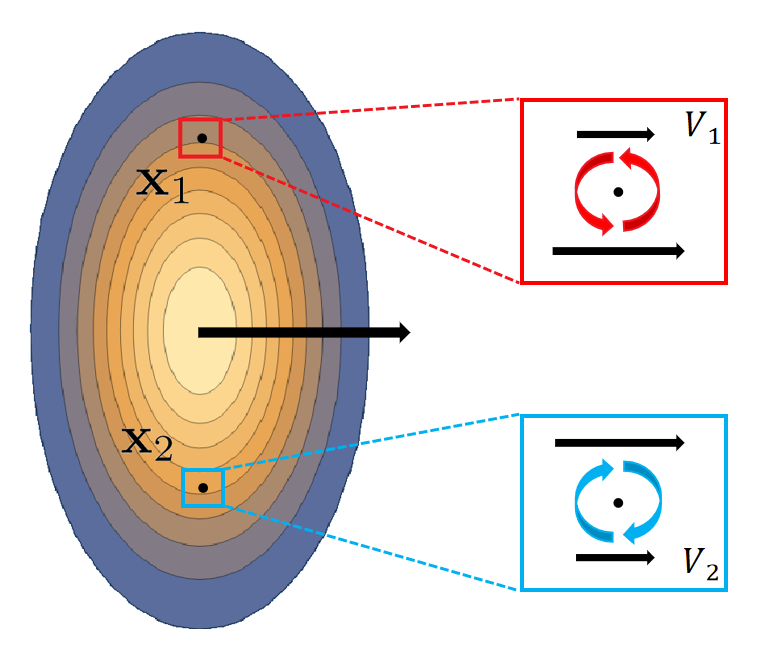
Figure 1: Local angular momentum density generated by an inhomogeneous current density.

On the other hand, $\mathcal{A}_{\mu}$ in Eq. (12) is interpreted as the spin angular-momentum density, which consists of two parts. The first part is an intrinsic spin density $\sim\text{tr}\left[n^{\mu}({\bf p})F\right]$, which is proportional to the polarization vector multiplied with the distribution function. The second part is a motion-induced part $\sim\text{tr}(L_{u_{0}}^{\mu\nu}\partial_{\nu}F)$, which is generated through the spin-orbit coupling. Considering a Gaussian-type particle number-density distribution moving to the right with momentum $\mathbf{p}$ at time $t=0$, cf. Fig. 1, the local current density is then given by ${\bf p}\,\text{tr}\left[F(\mathbf{x},p)\right]$. For the region $V_{1}$ in the vicinity of the point ${\bf x}_{1}$, the current density nearer to the center of the distribution is larger than that further away from the center, leading to a nonvanishing OAM

$${\bf L}_{V_{1}} =\int_{V_{1}}d^{3}{\bf x}^{\prime}\left({\bf x}^{\prime}-{\bf x}_{1}\right)\times{\bf p}\,\text{tr}\left[F({\bf x}^{\prime},p)\right]$$

$$\simeq-\frac{1}{3}{\bf p}\times\boldsymbol{\nabla}_{{\bf x}_{1}}\text{tr}[F({\bf x}_{1},p)]\int_{V_{1}}d^{3}{\bf x}^{\prime}\left({\bf x}^{\prime}-{\bf x}_{1}\right)^{2}\;,$$ (17)

where we have made a gradient expansion for $F({\bf x}^{\prime},p)$ near ${\bf x}_{1}$. By comparing $L_{V_{1}}$ with the OAM of a local vortex with kinetic vorticity $\boldsymbol{\omega}$,

$${\bf L}_{\boldsymbol{\omega}}=\frac{1}{3}{\boldsymbol{\omega}}E_{\bf p}\text{tr}[F({\bf x}_{1},p)]\int_{V_{1}}d^{3}{\bf x}^{\prime}\left({\bf x}^{\prime}-{\bf x}_{1}\right)^{2}\;,$$ (18)

one can find that the OAM generated by the inhomogeneous current density near point ${\bf x}_{1}$ corresponds to that of an anti-clockwise rotating vortex with

$${\boldsymbol{\omega}}=-\frac{{\bf p}\times\boldsymbol{\nabla}_{{\bf x}_{1}}\text{tr}[F({\bf x}_{1},p)]}{E_{\bf p}\text{tr}[F({\bf x}_{1},p)]}\;.$$ (19)

Similarly, the OAM near the point ${\bf x}_{2}$ is equivalent to the contribution of a clockwise rotating vortex, because the density gradient at $\mathbf{x}_{2}$ points in the opposite direction than that at point ${\bf x}_{1}$. Through the spin-orbit coupling, the OAM results in a nonvanishing spin density, i.e., the term $\sim\text{tr}(L_{u_{0}}^{\mu\nu}\partial_{\nu}F)$ in Eq. (12).

Lorentz transformation. —

We now study how the MVSD transforms under a Lorentz boost from the laboratory frame, characterized by the frame vector $u_{0}^{\mu}=(1,0,0,0)$, to a new reference frame called “$u$-frame” in the following, which moves with velocity $u^{\mu}=(\gamma,\gamma{\bf v})$ with respect to the laboratory frame. This Lorentz boost is denoted as $\Lambda_{uu_{0}}$ (without specifying the particular representation of the Lorentz group that this boost acts on).

The plane-wave state introduced in Eq. (1) transforms as

$$U(\Lambda_{uu_{0}})\left|{\bf p},s\right\rangle=\sum_{r}\left|{\bf p}^{\prime},r\right\rangle D_{rs}(R_{u,{\bf p}})\;,$$ (20)

where $U(\Lambda_{uu_{0}})$ is a unitary representation for $\Lambda_{uu_{0}}$ (appropriate for acting on the Fock-space state $\left|{\bf p},s\right\rangle$) and ${\bf p}^{\prime}$ is the spatial component of the momentum in the $u$-frame, satisfing $p^{\prime\mu}=\left(\Lambda_{uu_{0}}\right)_{\ \nu}^{\mu}p^{\nu}$. Note that in general a Lorentz boost changes the spin of a particle, which is also known as Wigner rotation $R_{u,{\bf p}}$. The latter is defined as the product of three Lorentz boosts, $R_{u,{\bf p}}\equiv\Lambda_{\text{rest},u}\Lambda_{uu_{0}}\Lambda_{u_{0},\text{rest}}$, where “rest” denotes the rest frame with $p_{\text{rest}}^{\mu}=\left(\Lambda_{\text{rest},u_{0}}\right)_{\ \nu}^{\mu}p^{\nu}=(m,{\bf 0})$. In Eq. (20), the Wigner rotation is encoded in the unitary $2\times 2$ matrix $D_{rs}(R_{u,{\bf p}})$ in spin space. For massless particles, this matrix is diagonal and reduces to a mere phase factor.

The transformation behavior of the Dirac spinors follows from Eq. (20),

$$\left(\Lambda_{uu_{0}}\right)_{\frac{1}{2}}u_{s}({\bf p})=\sum_{r}u_{r}({\bf p}^{\prime})D_{rs}(R_{u,{\bf p}})\;,$$ (21)

which gives

$$D_{rs}(R_{u,{\bf p}})=\frac{1}{2m}\bar{u}_{r}({\bf p}^{\prime})\left(\Lambda_{uu_{0}}\right)_{\frac{1}{2}}u_{s}({\bf p})\;,$$ (22)

where $\left(\Lambda_{uu_{0}}\right)_{\frac{1}{2}}$ is the spinor representation of the Lorentz boost $\Lambda_{uu_{0}}$.

Demanding that the density matrix in Eq. (2) transforms as $\rho^{\prime}=U(\Lambda_{uu_{0}})\rho\,U^{\dagger}(\Lambda_{uu_{0}})$ and then using Eq. (20), we obtain the transformation property of the MVSD in momentum space,

$$\tilde{f}^{\prime}(\mathbf{p}_{1}^{\prime},\mathbf{p}_{2}^{\prime})=D(R_{u,{\bf p}_{1}})\tilde{f}(\mathbf{p}_{1},\mathbf{p}_{2})D^{\dagger}(R_{u,{\bf p}_{2}})\;,$$ (23)

where $\tilde{f}^{\prime}$, $\mathbf{p}_{1}^{\prime}$, and $\mathbf{p}_{2}^{\prime}$ are quantities in the $u$-frame, with $p_{i}^{\prime\mu}=\left(\Lambda_{uu_{0}}\right)_{\ \nu}^{\mu}p_{i}^{\nu}$ for $i=1,2$. Here, both $D$ and $\tilde{f}$ are $2\times 2$ matrices, whose indices are omitted for the sake of simplicity. Substituting the above relation into Eq. (3), we derive

$$f^{\prime}(x^{\prime},p^{\prime}) =D(R_{u,{\bf p}})f(x,p)D^{\dagger}(R_{u,{\bf p}})$$

$$\!\!\!\!\!\!\!\!\!\!\!\!-\frac{i\hbar}{2}\left[\boldsymbol{\nabla}_{{\bf p}}D(R_{u,{\bf p}})\right]\cdot\left[\boldsymbol{\nabla}_{{\bf x}}f(x,p)\right]D^{\dagger}(R_{u,{\bf p}})$$

$$\!\!\!\!\!\!\!\!\!\!\!\!+\frac{i\hbar}{2}D(R_{u,{\bf p}})\left[f(x,p)\overleftarrow{\boldsymbol{\nabla}}_{{\bf x}}\right]\cdot\left[\boldsymbol{\nabla}_{{\bf p}}D^{\dagger}(R_{u,{\bf p}})\right]\;.$$ (24)

Given explicit expressions for the Dirac spinors, we can derive the matrix $D$ in Eq. (22). Then, we substitute $D$ into Eq. (24). The Lorentz transform of $F$, defined in Eq. (9), can be expressed with the help of Eq. (24) as

$$F^{\prime}=D(R_{u,{\bf p}})\left[F+\frac{\hbar}{2}\left\{\Delta_{u_{0}u}^{\mu},\partial_{\mu}F\right\}\right]D^{\dagger}(R_{u,{\bf p}})\;,$$ (25)

where

$$\Delta_{u_{0}u}^{\mu}\equiv\Delta_{u_{0}}^{\mu}-\Delta_{u}^{\mu}\;.$$ (26)

with the frame-dependent shift term being

$$\Delta_{u}^{\mu}\equiv-\frac{1}{m^{2}}S_{u}^{\mu\nu}p_{\nu}\equiv\frac{1}{m}L_{u}^{\mu\nu}n_{\nu}(\mathbf{p})\;.$$ (27)

Note that, if the $u$-frame is the rest frame of the particle, $u_{\mathrm{rest}}^{\mu}=p^{\mu}/m$, we have $\Delta_{u_{\mathrm{rest}}}^{\mu}=0$ and $\Delta_{u_{0}u_{\mathrm{rest}}}^{\mu}=\Delta_{u_{0}}^{\mu}$. Equation (25) states that, under a Lorentz boost, the transformed $F$ contains a rotation in spin space and an additional contribution from the gradient of $F$. The latter part arises because the magnetization current induced by an inhomogeneous spin angular momentum density and the OAM induced by an inhomogeneous current density are frame-dependent quantities. The shift term (27) has been studied for non-relativistic electron scattering off a central potential in ferromagnets in Ref. Berger (1970), and in this work we generalize it to the relativistic case.

We now discuss the behavior of $\mathcal{V}^{\mu}$ and $\mathcal{A}^{\mu}$ in Eqs. (11) and (12) under Lorentz transformations. In the $u$-frame, the vector current reads

$$\mathcal{V}^{\prime\mu}=C\,\text{tr}\left[\left(p^{\prime\mu}+\hbar S_{u_{0}}^{\prime\mu\nu}\partial^{\prime}_{\nu}\right)F^{\prime}(x^{\prime},p^{\prime})\right]\;,$$ (28)

where $S_{u_{0}}^{\prime\mu\nu}$ is the spin tensor (13) with $n^{\mu}(\mathbf{p})$ and $p^{\mu}$ replaced by $n^{\prime\mu}(\mathbf{p}^{\prime})$ and $p^{\prime\mu}$, respectively, while the frame vector $u_{0}^{\mu}=(1,0,0,0)$ is not transformed due to the frame dependence of $S_{u_{0}}^{\prime\mu\nu}$. We now replace all $u$-frame Lorentz tensors in Eq. (28) by laboratory-frame tensors, using $a^{\prime\mu}=(\Lambda_{uu_{0}})^{\mu}_{\ \nu}a^{\nu}$ and $u_{0}^{\mu}=(\Lambda_{uu_{0}})^{\mu}_{\ \nu}u^{\nu}$. The Lorentz transformation of the spin-polarization vector can be deduced from its definition (10) and the transformation behavior of the Dirac spinors (21),

$$n^{\prime\mu}({\bf p}^{\prime})=D(R_{u,\mathbf{p}})(\Lambda_{uu_{0}})^{\mu}_{\ \nu}n^{\nu}(\mathbf{p})D^{\dagger}(R_{u,\mathbf{p}})\;.$$ (29)

Then, using Eq. (25), the Schouten identity for $p^{\lambda}\epsilon^{\mu\nu\alpha\beta}$ Sheng et al. (2020), as well as $p\cdot n(\mathbf{p})=0$, up to first order in $\hbar$ Eq. (28) reads

$$\mathcal{V}^{\prime\mu}=(\Lambda_{uu_{0}})^{\mu}_{\ \nu}\left(\mathcal{V}^{\nu}+\hbar\,C\,\text{tr}\left\{\Delta_{u_{0}u}^{\nu}p\cdot\partial F\right\}\right)\;.$$ (30)

To lowest order in $\hbar$, the distribution function $F$ fulfills a Boltzmann equation of the form $p\cdot\partial F=\mathcal{C}[F]$, cf. Eq. (41) below. Then, in the absence of collisions, $\mathcal{C}[F]=0$, the second term in Eq. (30) vanishes, so the vector current transforms in a Lorentz-covariant manner Chen et al. (2015); Hattori et al. (2019b).

In order to ensure the covariance of $\mathcal{V}^{\mu}$ in the presence of collisions, an additional term

$$\delta\mathcal{V}^{\mu}=\hbar\,C\,\text{tr}\left(\Delta_{u_{0}\bar{u}}^{\mu}p\cdot\partial F\right)$$ (31)

needs to be added to $\mathcal{V}^{\mu}$ in Eq. (11), where $\bar{u}^{\mu}$ is an arbitrary frame vector and $\Delta^{\mu}_{\bar{u}}$, cf. Eq. (27), transforms as a Lorentz vector. Then, defining $\hat{\mathcal{V}}^{\mu}\equiv\mathcal{V}^{\mu}+\delta\mathcal{V}^{\mu}$ one can show that $\hat{\mathcal{V}}^{\prime\mu}=(\Lambda_{uu_{0}})^{\mu}_{\ \nu}\hat{\mathcal{V}}^{\nu}$ up to order $\mathcal{O}(\hbar)$, i.e., $\hat{\mathcal{V}}^{\mu}$ transforms as a Lorentz vector.

To prove the Lorentz covariance of the axial-vector current, an analogous calculation as in the vector case yields Hattori et al. (2019b)

$$\mathcal{A}^{\prime\mu}=(\Lambda_{uu_{0}})^{\mu}_{\ \nu}\,\mathcal{A}^{\nu}\;,$$ (32)

using Eqs. (27), (29), as well as the relation

$$\left\{n^{\mu}(\mathbf{p}),n^{\nu}(\mathbf{p})\right\}=-2\left(g^{\mu\nu}-\frac{p^{\mu}p^{\nu}}{m^{2}}\right)\;.$$ (33)

Equation (32) shows that the axial-vector current always transforms in a Lorentz-covariant manner, even in the case with collisions.

Collision term. —

Now we consider the case of binary elastic collisions. In the classical case, all incoming or outgoing particles have well-defined positions and the scattering process happens at one space-time point $x$. However, for quantum particles the position has a finite uncertainty and therefore particles can interact with each other over a finite distance. Such a nonlocal collision involves a finite OAM, which can be converted into the particle’s spin, or vice versa.

In the laboratory frame, the conserved angular-momentum tensor relative to a specific point $x_{0}^{\mu}$ is given by $J^{0\mu\nu}$,

$$J^{0\mu\nu}= \int\frac{d^{3}{\bf p}}{(2\pi\hbar)^{3}}\text{tr}\left\{\left[(x^{\mu}-x_{0}^{\mu})p^{\nu}\right.\right.$$

$$\left.\left.-(x^{\nu}-x_{0}^{\nu})p^{\mu}+\hbar S_{u_{0}}^{\mu\nu}\right]F(x,p)\right\}\;.$$ (34)

One can clearly identify the last term as the contribution from spin angular momentum and the remaining terms as the OAM part. However, note that the following identity holds up to order $\hbar$,

$$\Delta^{\mu}_{u_{0}u}p^{\nu}-\Delta^{\nu}_{u_{0}u}p^{\mu}+S^{\mu\nu}_{u_{0}}-S^{\mu\nu}_{u}=0\;,$$ (35)

which can be proved by employing Eqs. (26), (27), and the Schouten identity. Here $S_{u}^{\mu\nu}$ is the spin tensor defined in Eq. (13) with $u_{0}^{\mu}$ replaced by $u^{\mu}$. Then it is possible to express $J^{0\mu\nu}$ in another form with the help of the frame vector $u^{\mu}$,

$$J^{0\mu\nu}= \int\frac{d^{3}{\bf p}}{(2\pi\hbar)^{3}}\text{tr}\left\{\left[(x^{\mu}-x_{0}^{\mu}-\hbar\Delta^{\mu}_{u_{0}u})p^{\nu}\right.\right.$$

$$\left.\left.-(x^{\nu}-x_{0}^{\nu}-\hbar\Delta^{\nu}_{u_{0}u})p^{\mu}+\hbar S_{u}^{\mu\nu}\right]F(x,p)\right\}\;.$$ (36)

Using the Lorentz transform (25) of the MVSD, we can prove that the last term in Eq. (Collision term. —) is related to the spin angular momentum in the reference frame moving with velocity $u^{\mu}=(\gamma,\gamma{\bf v})$ relative to the laboratory frame,

$$\text{tr}[\hbar S^{\mu\nu}_{u}F(x,p)]=(\Lambda_{u_{0}u})^{\mu}_{\ \alpha}(\Lambda_{u_{0}u})^{\nu}_{\ \beta}\text{tr}[\hbar S^{\prime\alpha\beta}_{u_{0}}F^{\prime}(x^{\prime},p^{\prime})]\;,$$ (37)

where we have dropped terms of order $\mathcal{O}(\hbar^{2})$. We then conclude that the conserved angular momentum $J^{0\mu\nu}$ is independent of the reference frame, while the decomposition of $J^{0\mu\nu}$ into spin and OAM depends on the choice of $u^{\mu}$.

Assuming that, at leading order in $\hbar$, the MVSD satisfies a Boltzmann equation of the same form as in the classical case, $p\cdot\partial F(x,p)=\mathcal{C}[F]+\mathcal{O}(\hbar)$, one immediately obtains the requirement for angular-momentum conservation during collisions,

$$\int Dp\,\text{tr}\left\{\left[(x^{\mu}-x_{0}^{\mu}-\hbar\Delta^{\mu}_{u_{0}u})p^{\nu}\right.\right.$$

$$\left.\left.-(x^{\nu}-x_{0}^{\nu}-\hbar\Delta^{\nu}_{u_{0}u})p^{\mu}+\hbar S_{u}^{\mu\nu}\right]\mathcal{C}[F]\right\}=0\;.$$ (38)

In the massless case, there exists a special frame, the so-called “no-jump” frame Chen et al. (2015), where the incoming particles collide at the same position $x$. In our case of massive particles, the analogue is a frame, characterized by a frame vector $\bar{u}^{\mu}$, where the spin angular momentum and thus, by conservation of total angular momentum, also the OAM are separately conserved, i.e.,

$$\hbar\int Dp\,\text{tr}\left(S_{\bar{u}}^{\mu\nu}\mathcal{C}[F]\right)=0\;.$$ (39)

In this frame, the Boltzmann equation is assumed to take the same form as in the classical case,

$$\bar{p}\cdot\bar{\partial}\bar{F}(\bar{x},\bar{p})=\bar{\mathcal{C}}[\bar{F}]\;.$$ (40)

Then, using Eq. (25) we conclude that in the laboratory frame the Boltzmann equation reads

$$p\cdot\partial\left[F(x,p)+\frac{\hbar}{2}\left\{\Delta_{u_{0}\bar{u}}^{\mu},\partial_{\mu}F(x,p)\right\}\right]=\mathcal{C}[F]\;,$$ (41)

where the collision term $\mathcal{C}[F]$ is related to $\bar{\mathcal{C}}[\bar{F}]$ as

$$\bar{\mathcal{C}}[\bar{F}]=D(R_{\bar{u},{\bf p}})\mathcal{C}[F]D^{\dagger}(R_{\bar{u},{\bf p}})+\mathcal{O}(\hbar)\;.$$ (42)

Since the left-hand side of Eq. (41) is Hermitian, the collision term must also be Hermitian, $\mathcal{C}^{\dagger}[F]=\mathcal{C}[F]$. In the $\bar{u}$-frame, collisions are local, and the collision term $\bar{\mathcal{C}}[\bar{F}]$ has the same form as in the classical case. One can then show that, in the laboratory frame,

$$\mathcal{C}_{rs}[F] = \frac{1}{4}\sum_{r_{i},s_{i}}\int DP\mathcal{M}\left(p_{1},p_{2};s_{1},s_{2}\rightarrow p,p_{3};r_{0},r_{3}\right)$$ (43)

$$\times\mathcal{M}^{\ast}\left(p_{1},p_{2};r_{1},r_{2}\rightarrow p,p_{3};r,s_{3}\right)$$

$$\times\Biggl{\{}\tilde{F}_{r_{1}s_{1}}(p_{1})\tilde{F}_{r_{2}s_{2}}(p_{2})\left[\delta_{r_{0}s}-\tilde{F}_{r_{0}s}(p)\right]$$

$$\times\left[\delta_{r_{3}s_{3}}-\tilde{F}_{r_{3}s_{3}}(p_{3})\right]-\tilde{F}_{r_{0}s}(p)\tilde{F}_{r_{3}s_{3}}(p_{3})$$

$$\times\left[\delta_{r_{1}s_{1}}-\tilde{F}_{r_{1}s_{1}}(p_{1})\right]\left[\delta_{r_{2}s_{2}}-\tilde{F}_{r_{2}s_{2}}(p_{2})\right]\Biggr{\}}$$

$$+\text{h.c.}\;,$$

where the invariant integration measure $DP\equiv Dp_{1}Dp_{2}Dp_{3}\,(2\pi\hbar)^{4}\delta^{(4)}(p_{1}+p_{2}-p-p_{3})$ and “h.c” stands for the Hermitian conjugate (complex conjugate and interchanging $r$ and $s$) of the first term. In Eq. (43), the distribution function $\tilde{F}$ is defined as

$$\tilde{F}(x,p)\equiv F(x,p)+\frac{\hbar}{2}\left\{\Delta_{u_{0}\bar{u}}^{\mu},\partial_{\mu}F(x,p)\right\}\;,$$ (44)

and we suppressed the $x$-dependence of $\tilde{F}$ for the sake of simplicity. Under a Lorentz boost the transition amplitude transforms as

$$\bar{\mathcal{M}} =\sum_{s_{0}s_{1}s_{2}s_{3}}D_{s_{0}\bar{s}_{0}}D_{s_{3}\bar{s}_{3}}D_{\bar{s}_{1}s_{1}}^{\dagger}D_{\bar{s}_{2}s_{2}}^{\dagger}$$

$$\times\mathcal{M}\left(p_{1},p_{2};s_{1},s_{2}\rightarrow p,p_{3};s_{0},s_{3}\right)\;.$$ (45)

The Wigner rotation matrices in this equation partially cancel with those for the MVSDs in Eq. (25), which ensures that $\mathcal{C}[F]$ transforms as in Eq. (42). Note that the spin-orbit coupling enters the collision term through the presence of the shift term $\Delta_{u_{0}\bar{u}}^{\mu}$ in the definition of $\tilde{F}$, making the collision term nonlocal at first order in $\hbar$, cf. Refs. Weickgenannt et al. (2020, 2021); Sheng et al. (2021).

One can further check that the Boltzmann equation (41) fulfills the local conservation law for total angular momentum,

$$\hbar\partial_{\lambda}S^{\lambda\mu\nu}+T^{\mu\nu}-T^{\nu\mu}$$

$$=-2\hbar\int Dp\,\text{tr}\left(S_{\bar{u}}^{\mu\nu}\mathcal{C}[F]\right)+\mathcal{O}(\hbar^{2})=0\;,$$ (46)

where $S^{\lambda\mu\nu}$ is the canonical spin angular-momentum tensor defined above, $T^{\mu\nu}\equiv\int d^{4}p\,p^{\mu}\hat{\mathcal{V}}^{\nu}$, and $S_{\bar{u}}^{\mu\nu}$ is the spin tensor defined in Eq. (13) with $u_{0}^{\mu}$ replaced by $\bar{u}^{\mu}$. We emphasize that in the last line in Eq. (46) we have used Eq. (39), which demands that the spin is conserved in collisions in the $\bar{u}$-frame.

Local thermodynamical equilibrium. —

Usually, local thermodynamical equilibrium is defined by demanding that the collision term vanishes. This requirement leads to the solution $\tilde{F}(x,p)=f_{FD}(x,p;\delta E)$, with the Fermi-Dirac distribution defined as

$$f_{FD}(x,p;\delta E)\equiv\left\{1+\exp[(u\cdot p+\delta E-\mu)/T]\right\}^{-1}\;,$$ (47)

where the energy shift $\delta E\equiv\hbar S^{\mu\nu}_{\bar{u}}\Omega_{\mu\nu}$, with $\Omega_{\mu\nu}$ being the spin potential. Using Eq. (44) the MVSD in the lab frame is then up to order $\mathcal{O}(\hbar)$ given by

$$F(x,p)=f_{FD}(x,p;\delta E)-\frac{\hbar}{2}\left\{\Delta_{u_{0}\bar{u}}^{\mu},\partial_{\mu}f_{FD}(x,p;\delta E)\right\}\;.$$ (48)

With Eqs. (12), (14), (26), and (33) one then computes the axial-vector component of the Wigner function as

$$\mathcal{A}^{\mu} =C\,\text{tr}\left\{\left[mn^{\mu}({\bf p})\,\frac{}{}\right.\right.$$

$$\left.\left.-\frac{\hbar}{2(\bar{u}\cdot p)}\epsilon^{\mu\nu\alpha\beta}\bar{u}_{\nu}p_{\alpha}\partial_{\beta}\right]f_{FD}(x,p;\delta E)\right\}\;,$$ (49)

which agrees with the result that includes the thermal-shear contribution Wang et al. (2020); Becattini et al. (2021a); Liu and Yin (2021); Fu et al. (2021); Becattini et al. (2021b); Yi et al. (2021); Buzzegoli (2021); Liu and Huang (2021). In the massless limit, Eq. (49) smoothly reduces to the result of CKT Chen et al. (2015); Hidaka et al. (2018), which can be proved by replacing $mn^{\mu}({\bf p})\rightarrow p^{\mu}$.

Conclusions. —

In this work, we have derived a matrix-valued spin-dependent distribution function (MVSD) $F(x,p)$ for quantum particles, which describes the particle number density and intrinsic spin density in phase space. A physical interpretation of the MVSD is provided by expressing the vector and axial-vector components of the Wigner function in terms of $F(x,p)$. In an inhomogeneous system, the magnetization current and the OAM contained in an inhomogeneous momentum distribution result in nontrivial Lorentz-transformation properties for $F(x,p)$: in addition to the ordinary Wigner rotation, $F(x,p)$ undergoes a matrix-valued shift $\Delta_{u_{0}u}^{\mu}$ in space-time. This term ensures that the axial-vector component, and in the collisionless case, also the vector component of the Wigner function transform in a Lorentz-covariant manner. Including collisions, the vector component requires an additional contribution to preserve Lorentz covariance. Assuming the existence of a $\bar{u}$-frame where spin is a collisional invariant, and using the Lorentz transformation properties of the MVSD, we further constructed a manifestly covariant Boltzmann equation including nonlocal terms, which give rise to spin-orbit coupling during collisions. In the $\bar{u}$–frame, we derive a local-equilibrium solution for $F(x,p)$ and for the axial-vector component $\mathcal{A}^{\mu}$. The Lorentz-covariant Boltzmann equation derived in this work provides a solid foundation for studying spin dynamics in heavy-ion collisions and, ultimately, the long-sought means to solve the sign problem of the longitudinal polarization.

References

- Liang and Wang (2005a) Z.-T. Liang and X.-N. Wang, Phys. Rev. Lett. 94, 102301 (2005a), [Erratum: Phys. Rev. Lett.96,039901(2006)], arXiv:nucl-th/0410079 [nucl-th] .
- Liang and Wang (2005b) Z.-T. Liang and X.-N. Wang, Phys. Lett. B 629, 20 (2005b), arXiv:nucl-th/0411101 .
- Voloshin (2004) S. A. Voloshin, (2004), arXiv:nucl-th/0410089 .
- Adamczyk et al. (2017) L. Adamczyk et al. (STAR), Nature 548, 62 (2017), arXiv:1701.06657 [nucl-ex] .
- Adam et al. (2018) J. Adam et al. (STAR), Phys. Rev. C98, 014910 (2018), arXiv:1805.04400 [nucl-ex] .
- Becattini et al. (2013) F. Becattini, V. Chandra, L. Del Zanna, and E. Grossi, Annals Phys. 338, 32 (2013), arXiv:1303.3431 [nucl-th] .
- Karpenko and Becattini (2017) I. Karpenko and F. Becattini, Eur. Phys. J. C 77, 213 (2017), arXiv:1610.04717 [nucl-th] .
- Wei et al. (2019) D.-X. Wei, W.-T. Deng, and X.-G. Huang, Phys. Rev. C 99, 014905 (2019), arXiv:1810.00151 [nucl-th] .
- Adam et al. (2019) J. Adam et al. (STAR), Phys. Rev. Lett. 123, 132301 (2019), arXiv:1905.11917 [nucl-ex] .
- Florkowski et al. (2019a) W. Florkowski, A. Kumar, R. Ryblewski, and R. Singh, Phys. Rev. C 99, 044910 (2019a), arXiv:1901.09655 [hep-ph] .
- Sun and Ko (2019) Y. Sun and C. M. Ko, Phys. Rev. C 99, 011903 (2019), arXiv:1810.10359 [nucl-th] .
- Florkowski et al. (2019b) W. Florkowski, A. Kumar, R. Ryblewski, and A. Mazeliauskas, Phys. Rev. C 100, 054907 (2019b), arXiv:1904.00002 [nucl-th] .
- Becattini et al. (2019a) F. Becattini, G. Cao, and E. Speranza, Eur. Phys. J. C 79, 741 (2019a), arXiv:1905.03123 [nucl-th] .
- Xia et al. (2019) X.-L. Xia, H. Li, X.-G. Huang, and H. Z. Huang, Phys. Rev. C 100, 014913 (2019), arXiv:1905.03120 [nucl-th] .
- Wu et al. (2019) H.-Z. Wu, L.-G. Pang, X.-G. Huang, and Q. Wang, Phys. Rev. Research. 1, 033058 (2019), arXiv:1906.09385 [nucl-th] .
- Liu et al. (2020) S. Y. F. Liu, Y. Sun, and C. M. Ko, Phys. Rev. Lett. 125, 062301 (2020), arXiv:1910.06774 [nucl-th] .
- Becattini et al. (2021a) F. Becattini, M. Buzzegoli, and A. Palermo, Phys. Lett. B 820, 136519 (2021a), arXiv:2103.10917 [nucl-th] .
- Liu and Yin (2021) S. Y. F. Liu and Y. Yin, JHEP 07, 188 (2021), arXiv:2103.09200 [hep-ph] .
- Fu et al. (2021) B. Fu, S. Y. F. Liu, L. Pang, H. Song, and Y. Yin, Phys. Rev. Lett. 127, 142301 (2021), arXiv:2103.10403 [hep-ph] .
- Becattini et al. (2021b) F. Becattini, M. Buzzegoli, A. Palermo, G. Inghirami, and I. Karpenko, (2021b), arXiv:2103.14621 [nucl-th] .
- Yi et al. (2021) C. Yi, S. Pu, and D.-L. Yang, (2021), arXiv:2106.00238 [hep-ph] .
- Zhang et al. (2019) J.-j. Zhang, R.-h. Fang, Q. Wang, and X.-N. Wang, Phys. Rev. C 100, 064904 (2019), arXiv:1904.09152 [nucl-th] .
- Li and Yee (2019) S. Li and H.-U. Yee, Phys. Rev. D 100, 056022 (2019), arXiv:1905.10463 [hep-ph] .
- Liu and Huang (2020) Y.-C. Liu and X.-G. Huang, Nucl. Sci. Tech. 31, 56 (2020), arXiv:2003.12482 [nucl-th] .
- Yang et al. (2020) D.-L. Yang, K. Hattori, and Y. Hidaka, JHEP 07, 070 (2020), arXiv:2002.02612 [hep-ph] .
- Weickgenannt et al. (2020) N. Weickgenannt, E. Speranza, X.-l. Sheng, Q. Wang, and D. H. Rischke, (2020), arXiv:2005.01506 [hep-ph] .
- Li (2021) S. Li, Nucl. Phys. A 1005, 121977 (2021), arXiv:2003.00106 [hep-ph] .
- Manuel and Torres-Rincon (2021) C. Manuel and J. M. Torres-Rincon, Phys. Rev. D 103, 096022 (2021), arXiv:2101.05832 [hep-ph] .
- Weickgenannt et al. (2021) N. Weickgenannt, E. Speranza, X.-l. Sheng, Q. Wang, and D. H. Rischke, (2021), arXiv:2103.04896 [nucl-th] .
- Sheng et al. (2021) X.-L. Sheng, N. Weickgenannt, E. Speranza, D. H. Rischke, and Q. Wang, Phys. Rev. D 104, 016029 (2021), arXiv:2103.10636 [nucl-th] .
- Lin (2021) S. Lin, (2021), arXiv:2109.00184 [hep-ph] .
- Florkowski et al. (2018a) W. Florkowski, B. Friman, A. Jaiswal, and E. Speranza, Phys. Rev. C 97, 041901 (2018a), arXiv:1705.00587 [nucl-th] .
- Florkowski et al. (2018b) W. Florkowski, B. Friman, A. Jaiswal, R. Ryblewski, and E. Speranza, Phys. Rev. D 97, 116017 (2018b), arXiv:1712.07676 [nucl-th] .
- Montenegro et al. (2017) D. Montenegro, L. Tinti, and G. Torrieri, Phys. Rev. D 96, 056012 (2017), [Addendum: Phys.Rev.D 96, 079901 (2017)], arXiv:1701.08263 [hep-th] .
- Florkowski et al. (2019c) W. Florkowski, R. Ryblewski, and A. Kumar, Prog. Part. Nucl. Phys. 108, 103709 (2019c), arXiv:1811.04409 [nucl-th] .
- Florkowski et al. (2018c) W. Florkowski, E. Speranza, and F. Becattini, Acta Phys. Polon. B 49, 1409 (2018c), arXiv:1803.11098 [nucl-th] .
- Becattini et al. (2019b) F. Becattini, W. Florkowski, and E. Speranza, Phys. Lett. B 789, 419 (2019b), arXiv:1807.10994 [hep-th] .
- Hattori et al. (2019a) K. Hattori, M. Hongo, X.-G. Huang, M. Matsuo, and H. Taya, Phys. Lett. B 795, 100 (2019a), arXiv:1901.06615 [hep-th] .
- Bhadury et al. (2021) S. Bhadury, W. Florkowski, A. Jaiswal, A. Kumar, and R. Ryblewski, Phys. Lett. B 814, 136096 (2021), arXiv:2002.03937 [hep-ph] .
- Montenegro and Torrieri (2020) D. Montenegro and G. Torrieri, Phys. Rev. D 102, 036007 (2020), arXiv:2004.10195 [hep-th] .
- Li et al. (2021) S. Li, M. A. Stephanov, and H.-U. Yee, Phys. Rev. Lett. 127, 082302 (2021), arXiv:2011.12318 [hep-th] .
- Son and Yamamoto (2012) D. T. Son and N. Yamamoto, Phys. Rev. Lett. 109, 181602 (2012), arXiv:1203.2697 [cond-mat.mes-hall] .
- Stephanov and Yin (2012) M. A. Stephanov and Y. Yin, Phys. Rev. Lett. 109, 162001 (2012), arXiv:1207.0747 [hep-th] .
- Chen et al. (2013) J.-W. Chen, S. Pu, Q. Wang, and X.-N. Wang, Phys. Rev. Lett. 110, 262301 (2013), arXiv:1210.8312 [hep-th] .
- Chen et al. (2014a) J.-Y. Chen, D. T. Son, M. A. Stephanov, H.-U. Yee, and Y. Yin, Phys. Rev. Lett. 113, 182302 (2014a), arXiv:1404.5963 [hep-th] .
- Chen et al. (2015) J.-Y. Chen, D. T. Son, and M. A. Stephanov, Phys. Rev. Lett. 115, 021601 (2015), arXiv:1502.06966 [hep-th] .
- Hidaka et al. (2017) Y. Hidaka, S. Pu, and D.-L. Yang, Phys. Rev. D 95, 091901 (2017), arXiv:1612.04630 [hep-th] .
- Sheng et al. (2020) X.-L. Sheng, Q. Wang, and X.-G. Huang, Phys. Rev. D 102, 025019 (2020), arXiv:2005.00204 [hep-ph] .
- Gao and Liang (2019) J.-H. Gao and Z.-T. Liang, Phys. Rev. D 100, 056021 (2019), arXiv:1902.06510 [hep-ph] .
- Weickgenannt et al. (2019) N. Weickgenannt, X.-L. Sheng, E. Speranza, Q. Wang, and D. H. Rischke, Phys. Rev. D100, 056018 (2019), arXiv:1902.06513 [hep-ph] .
- Wang et al. (2019) Z. Wang, X. Guo, S. Shi, and P. Zhuang, Phys. Rev. D 100, 014015 (2019), arXiv:1903.03461 [hep-ph] .
- Hattori et al. (2019b) K. Hattori, Y. Hidaka, and D.-L. Yang, Phys. Rev. D 100, 096011 (2019b), arXiv:1903.01653 [hep-ph] .
- Wigner (1939) E. P. Wigner, Annals Math. 40, 149 (1939), [Reprint: Nucl. Phys. Proc. Suppl.6,9(1989)].
- Kim and Wigner (1987) Y. S. Kim and E. P. Wigner, J. Math. Phys. 28, 1175 (1987).
- Kim and Wigner (1990) Y. S. Kim and E. P. Wigner, J. Math. Phys. 31, 55 (1990).
- Hidaka et al. (2018) Y. Hidaka, S. Pu, and D.-L. Yang, Phys. Rev. D 97, 016004 (2018), arXiv:1710.00278 [hep-th] .
- Becattini and Tinti (2010) F. Becattini and L. Tinti, Annals Phys. 325, 1566 (2010), arXiv:0911.0864 [gr-qc] .
- Heinz (1983) U. W. Heinz, Phys. Rev. Lett. 51, 351 (1983).
- Vasak et al. (1987) D. Vasak, M. Gyulassy, and H. T. Elze, Annals Phys. 173, 462 (1987).
- Itzykson and Zuber (1980) C. Itzykson and J. Zuber, Quantum Field Theory, International Series In Pure and Applied Physics (McGraw-Hill, New York, 1980).
- Chen et al. (2014b) J.-W. Chen, J.-y. Pang, S. Pu, and Q. Wang, Phys. Rev. D 89, 094003 (2014b), arXiv:1312.2032 [hep-th] .
- Pryce (1948) M. H. L. Pryce, Proc. Roy. Soc. Lond. A 195, 62 (1948).
- Bacry (1988) H. Bacry, Localizability and Space in Quantum Physics, Vol. 308 (1988).
- Rivas (2002) M. Rivas, Kinematical Theory of Spinning Particles, Vol. 116 (Springer Netherlands, 2002).
- Lorcé (2021) C. Lorcé, Eur. Phys. J. C 81, 413 (2021), arXiv:2103.10100 [hep-ph] .
- Berger (1970) L. Berger, Phys. Rev. B 2, 4559 (1970).
- Wang et al. (2020) Z. Wang, X. Guo, and P. Zhuang, (2020), arXiv:2009.10930 [hep-th] .
- Buzzegoli (2021) M. Buzzegoli, (2021), arXiv:2109.12084 [nucl-th] .
- Liu and Huang (2021) Y.-C. Liu and X.-G. Huang, (2021), arXiv:2109.15301 [nucl-th] .