Channel Estimation and Projection for RIS-assisted MIMO Using Zadoff-Chu Sequences

Abstract

The reconfigurable intelligent surface (RIS) technology is a promising enabler for millimeter wave (mmWave) wireless communications, as it can potentially provide spectral efficiency comparable to the conventional massive multiple-input multiple-output (MIMO) but with significantly lower hardware complexity. In this paper, we focus on the estimation and projection of the uplink RIS-aided massive MIMO channel, which can be time-varying. We propose to let the user equipments (UE) transmit Zadoff-Chu (ZC) sequences and let the base station (BS) conduct maximum likelihood (ML) estimation of the uplink channel. The proposed scheme is computationally efficient: it uses ZC sequences to decouple the estimation of the frequency and time offsets; it uses the space-alternating generalized expectation-maximization (SAGE) method to reduce the high-dimensional problem due to the multipaths to multiple lower-dimensional ones per path. Owing to the estimation of the Doppler frequency offsets, the time-varying channel state can be projected, which can significantly lower the overhead of the pilots for channel estimation. The numerical simulations verify the effectiveness of the proposed scheme.

I Introduction

Although the millimeter wave (mmWave) communication technology can provide abundant frequency bandwidth, it suffers from large pathloss. The massive multi-input multi-output (MMO) can be used to compensate for the pathloss with its large array gain; thus, mmWave massive MIMO has been intensively researched in the past several years (see [1], [2], [3] and the references therein). More recently, the reconfigurable intelligent surface (RIS) technology [4] has been introduced to wireless communication systems [5]. Compared with the conventional massive MIMO technology, the RIS-assisted MIMO allows for incorporating a very large number (thousands or even more) of reflection elements, leading to the so-called extreme massive MIMO with very large array gain [6]. As a passive device, the RIS can customize favorable wireless propagation environments with limited power consumption. Hence, it is envisioned that the combination of the mmWave and RIS technologies will be one of the keys to the beyond fifth-generation (B5G) wireless communications [7].

It is usually a prerequisite to have the channel state information (CSI) for reaping the great gain of the RIS-assisted massive MIMO. But the CSI is challenging to estimate due to the high dimensionality of the RIS. The similar issue also occurs in the mmWave phase shifter network (PSN) based hybrid massive MIMO scenario [8], [9]. In [10], Mishra et al. proposed a least square (LS) based channel estimation method for RIS-aided MIMO. A method using sparse matrix factorization and matrix completion was presented in [11]. However, both methods assumed a frequency-flat channel, which may not be the case in a real-world environment. Using the sparsity of the RIS channel, Wan, et al. proposed a compressive sensing (CS) based algorithm to estimate the frequency-selective channel [12], but the CS-based broadband channel estimation did not appear robust in different simulation scenarios. In [13], Zheng et al. also considered the scenario of the wide-band and frequency-selective channels. Assuming high channel correlation between the adjacent elements of the RIS, they proposed to group the adjacent elements into some sub-surfaces to reduce the dimension of the channel estimation problem [13]. But such elements-grouping would cause performance degradation, because the reflection coefficients of all the elements in one group have to be set the same [13]. The channel estimation based on the RIS-element-grouping was extended to the multi-user scenario in [14] and the time-varying channel scenario [15]. Both [13] and [14] made the restrictive assumption that the access point is only equipped with a single antenna. All the algorithms proposed in [13], [14] and [15] require that the number of training sequences increased linearly with the number of the elements (or the subsurface) of the RIS, which may cause too much pilot overhead in practice. In [16], Mao et al. considered the estimation of a time-variant frequency-flat channels, and employed Kalman filtering to estimate the time-varying channel.

In this paper, we investigate the uplink channel estimation for the RIS aided massive MIMO-OFDM system in a multipath environment. We consider the scenario where the RIS is placed close to the antennas of the base station (BS); thus, the RIS-to-BS channel can be assumed to be line-of-sight (LOS), frequency-flat, static, and hence is estimated a priori. This assumption is realistic and was also made in [12, 17]. Therefore, we focus on the estimation of the UE-to-RIS channel and the UE-to-BS (direct link) channel, which can be frequency selective and fast time-varying. In contrast, all the aforementioned papers only considered static RIS channels.

We propose to parameterize the multipath channel by a set of the directions of arrival (DOA), the time delays, the channel gains, and the Doppler frequency offsets. As a prominent feature of this work, introducing the Doppler frequency offsets into the model enables projection of the time-varying channel and henceforth reduces the pilots needed for channel estimation, which can help solve the pilot contamination issue [18].

We propose to use Zadoff-Chu (ZC) sequences as the pilots and exploit ZC’s unique property of time-delay and frequency offset ambiguity: That is, a ZC sequence with a time delay appears like one with frequency offset. Indeed, this property was exploited in [19] to simplify the two-dimensional problem of joint time delay-frequency offset estimation into a problem that can be efficiently solved via two one-dimensional fast Fourier transforms (FFT), based on a conjugate pair of ZC sequences. The ZC sequences’ time delay and frequency offset ambiguity is also exploited in this paper to reduce the computational complexity of channel estimation.

We let the UE transmit the ZC sequence multiple times, during which the reflection phases of the RIS will be varied. Based on the multiple sets of received samples, the channel parameters can be estimated. By exploiting the ZC sequence’s time delay-frequency offset ambiguity, we devise an FFT-based fast algorithm for joint estimation of the channel parameters. To tackle the multipath scenario, we use the space-alternating generalized expectation-maximization (SAGE) method [20] to decompose the multipath problem into multiple single-path subproblems. For each single path, the ML estimation consists of two steps: i) a fast initialization of the parameter estimates using FFTs; ii) the refinement for super-resolution estimation using Newton’s iterative method.

The main contributions of this paper are summarized as follows.

• we propose to use ZC sequences as the pilots, and devise a computationally efficient FFT-based channel estimation algorithm by exploiting the ambiguity of the time delay-frequency offset of the ZC sequences;

• the proposed algorithm can achieve super-resolution maximum likelihood (ML) parameters estimation for the frequency selective multipath channel, which leads to channel estimation with the root mean square error (RMSE) performance approaching the Cramer-Rao bound (CRB);

• with the estimated Doppler frequency offsets, the time-varying channel state can be projected to greatly reduce the pilot overhead for channel estimation, and thus help mitigate the pilot contamination in massive MIMO communications.

The remainder of this paper is organized as follows. Section II establishes the signal model and formulates the channel estimation problem based on RIS. Section III derives the solution to the channel estimation problem in the single-path case when the UE-BS channel is blocked. Based on the single-path solution, we further propose to apply the SAGE method to the multipath case. Section IV addresses the more general case where the direct channel link between the UE and the BS exists. Numerical examples are given in Section V and conclusions are made in Section VI.

Notations: $(\cdot)^{T}$, $(\cdot)^{*}$ and $(\cdot)^{H}$ stand for transpose, conjugate and Hermitian transpose, respectively. $\otimes$ denotes Kronecker product and $\odot$ denotes Hadamard (element-wise) product. ${\mathbb{Z}}$ is the set of integers, ${\mathbb{R}}$ is the set of real numbers, and $\mathbb{C}^{N\times K}$ is the set of $N\times K$ complex matrices. $\mathop{\rm diag}({\bf a})$ denotes a diagonal matrix with vector ${\bf a}$ being its diagonal and ${\mbox{vec}}(\cdot)$ denotes a vectorization operation to a matrix by stacking the columns of the matrix into a long column-vector. $\left\arrowvert\cdot\right\arrowvert$ stand for absolute value, $\|\cdot\|_{F}$ stands for the Frobenius norm, and $\left\Arrowvert\cdot\right\Arrowvert$ the $l_{2}$ norm. $\mathop{\rm Re}\{\cdot\}$ and $\mathop{\rm Im}\{\cdot\}$ stands for taking the real and imaginary part, respectively. $[\cdot]_{i,j}$ denotes the $(i,j)$th element of a matrix.

II Signal Model and Problem Formulation

II-A Signal Model

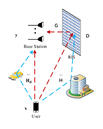
Figure 1: A RIS aided massive MIMO wireless communication system.

An RIS aided massive MIMO wireless communication system consists of a BS, a RIS, and a UE, as shown in Fig. 1, where the BS is connected to the UE through the direct link and the reflections of the RIS. Given that the RIS is a planar uniform rectangular array (URA) of $P$ rows and $Q$ columns. The array response of the RIS with respect to a signal from angle $(\theta,\varphi)$ can be represented by ${\bf A}(\theta,\varphi)\in{\mathbb{C}}^{P\times Q}$, whose entries are [21]

$$\left[{\bf A}(\theta,\varphi)\right]_{pq}=e^{-j\frac{2\pi}{\lambda}(q-1)d_{x}\sin\varphi\cos\theta+j\frac{2\pi}{\lambda}(p-1)d_{z}\cos\varphi},$$

$$p=1,2,\cdots,P,q=1,2,\cdots,Q,$$ (1)

where $\lambda$ denotes the wavelength of the carrier frequency, $d_{x}$ and $d_{z}$ represent the inter-element spacing along the horizontal and vertical direction of the RIS, respectively.

The array response of the $M_{r}$-antenna BS with respect to a signal from angle $\overline{\theta}$ can be represented by

$$\left[{\bf c}(\overline{\theta})\right]_{m}=e^{-j\frac{2\pi}{\lambda}(m-1)\bar{d}_{x}\cos\overline{\theta}}\in{\mathbb{C}}^{M_{r}\times 1},m=1,2,\cdots,M_{r},$$ (2)

where $\bar{d}_{x}$ is the inter-antenna distance of the BS array.

In the uplink channel, while the single-antenna UE transmits a continuous-time signal $x(t)$, the BS receives the signal

$${\bf y}(t) ={\bf G}{\bf D}\int{\bf H}(\tau,t)x(t-\tau)d\tau$$

$$+\int{\bf H}_{d}(\tau,t)x(t-\tau)d\tau+{\bf z}(t),$$ (3)

where ${\bf G}\in{\mathbb{C}}^{M_{r}\times M}$ is the RIS-to-BS channel with $M=PQ$ being the number of the elements of the RIS, ${\bf D}=\mathop{\rm diag}\{e^{j\phi_{1}},\ldots,e^{j\phi_{M}}\}$ with the diagonal represents the reflection phases of the RIS elements, ${\bf H}(t,\tau)$ is the time-varying multipath channel between the UE and the RIS, and ${\bf H}_{d}(t,\tau)$ is the time-varying multipath channel between the UE and the BS, ${\bf z}(t)\sim{\cal CN}(0,\sigma_{z}^{2}{\bf I}_{M_{r}})$ is the additive white Gaussian noise. Throughout this paper, we assume that the antennas of the BS are placed close to the RIS so that the channel ${\bf G}$ is frequency flat and static. Indeed, we can expect a steady LOS-path between the RIS and the BS, while the NLOS paths are much weaker than the LOS paths in the mmWave frequency band as shown in [22]. Therefore, one can construct the LOS part based on the position of the RIS relative to the BS. The same assumption that ${\bf G}$ is known a priori is also made in [12]. This paper focuses on estimating the UE-to-RIS channel

$${\bf H}(\tau,t)= \sum_{u=1}^{U}{\bf h}_{u}(t)\delta(\tau-\tau_{u}),$$ (4)

and the UE-to-BS channel

$${\bf H}_{d}(\tau,t)= \sum_{d=1}^{D}{\bf h}_{d}(t)\delta(\tau-\overline{\tau}_{d}).$$ (5)

Inserting (4) and (5) into (II-A) yields

$${\bf y}(t)={\bf G}{\bf D}\sum_{u=1}^{U}{\bf h}_{u}(t)x(t-\tau_{u})+\sum_{d=1}^{D}{\bf h}_{d}(t)x(\tau-\overline{\tau}_{d})+{\bf z}(t).$$ (6)

As the Doppler frequency spread is proportional to $\frac{v}{C}f_{c}$ – where $v$ is the UE’s mobility speed, $C$ is the speed-of-light, and $f_{c}$ is the carrier frequency – the large $f_{c}$ of the mmWave makes it necessary to model the channel as time-varying. To estimate the time-varying and high-dimensional channels ${\bf H}(\tau,t)$ and ${\bf H}_{d}(\tau,t)$ will apparently entail a large overhead of training sequences. To reduce the overhead, we propose to parameterize the time-varying channel as follows.

Denote ${\bf a}(\theta_{u},\varphi_{u})\triangleq{\mbox{vec}}({\bf A}(\theta_{u},\varphi_{u}))\in{\mathbb{C}}^{M}$, the array response of the $u$th path in (6) can be represented as

$${\bf h}_{u}(t)=\beta_{u}{\bf a}(\theta_{u},\varphi_{u})e^{j2\pi\xi_{u}t},$$ (7)

where $\beta_{u}$ is the complex-valued multipath gain, and $\xi_{u}$ is the Doppler frequency offset. The array response of the $d$th path in (6) can be represented as

$${\bf h}_{d}(t)=\alpha_{d}{\bf c}(\overline{\theta}_{u})e^{j2\pi\overline{\xi}_{d}t},$$ (8)

where $\alpha_{d}$ is the complex-valued multipath gain, and $\overline{\xi}_{d}$ is the Doppler frequency offset. Thus, we rewrite (6) to be

$${\bf y}(t)={\bf G}{\bf D}\sum_{u=1}^{U}\beta_{u}{\bf a}(\theta_{u},\varphi_{u})x(t-\tau_{u})e^{j2\pi\xi_{u}t}$$

$$+\sum_{d=1}^{D}\alpha_{d}{\bf c}(\overline{\theta}_{d})x(t-\overline{\tau}_{d})e^{j2\pi\overline{\xi}_{d}t}+{\bf z}(t).$$ (9)

The sampled signal at the output of the receiver’s analog-to-digital converters (ADC) is

$${\bf y}(n)={\bf G}{\bf D}\sum_{u=1}^{U}\beta_{u}{\bf a}(\theta_{u},\varphi_{u})x(n-\tau_{u})e^{j2\pi\xi_{u}n}$$

$$+\sum_{d=1}^{D}\alpha_{d}{\bf c}(\overline{\theta}_{d})x(n-\overline{\tau}_{d})e^{j2\pi\overline{\xi}_{d}n}+{\bf z}(n),n\in{\mathbb{Z}},$$ (10)

where we denote without loss of generality the Nyquist sampling interval $T_{s}=1$ for notational simplicity, but $\tau_{u}\in{\mathbb{R}}$ and $\overline{\tau}_{d}\in{\mathbb{R}}$ are not necessarily integers.

To improve the channel estimation, we change the reflection phases of the RIS for $K$ times, each corresponding to the transmission of a pilot with length $L$. Given that the channel parameters are static during the $K$ observations (note that a time-varying channel can be represented with static parameters), the BS receives

$${\bf y}_{k}(n) ={\bf W}(\Phi_{k})\sum_{u=1}^{U}\beta_{u}e^{j2\pi\xi_{u}(k-1)N}{\bf a}(\theta_{u},\varphi_{u})x(n-\tau_{u})$$

$$\times e^{j2\pi\xi_{u}n}+\sum_{d=1}^{D}\alpha_{d}e^{j2\pi\overline{\xi}_{d}(k-1)N}{\bf c}(\overline{\theta}_{d})x(n-\overline{\tau}_{d})$$

$$\times e^{j2\pi\overline{\xi}_{d}n}+{\bf z}_{k}(n),k=1,2,\cdots,K,$$ (11)

where ${\bf W}(\Phi_{k})\triangleq{\bf G}{\bf D}(\Phi_{k})$ with $\Phi_{k}$ being the phase of all elements of the RIS for the $k$th observation, and $N$ is the length of the OFDM symbol.

For each observation, we assume that $L$ samples, with indices from $-L/2$ to $L/2-1$, are processed [if $L$ is an odd number, the indices are from $-(L-1)/2$ to $(L-1)/2$]. The index range differs from the convention to cater to the proposed special design of the pilot $x(t)$, as we will see soon.

By formatting ${\bf y}_{k}(n)$ into the matrices

$$\begin{split}&{\bf Y}_{k}\!=\![{\bf y}_{k}(-\frac{L}{2}),{\bf y}_{k}(-\frac{L}{2}+1),\dots,{\bf y}_{k}(\frac{L}{2}-1)]\!\in\mathbb{C}^{M_{r}\times L},\\ \mbox{and}\\ &{\bf Z}_{k}=\left[{\bf z}_{k}(-L/2),{\bf z}_{k}(-L/2+1),\cdots,{\bf z}_{k}(L/2-1)\right],\end{split}$$ (12)

we have from (II-A) that

$${\bf Y}_{k}\!=\!{\bf W}(\Phi_{k})\sum_{u=1}^{U}{\bf a}(\theta_{u},\varphi_{u})\beta_{u}e^{j2\pi\xi_{u}(k-1)N}\left({\bf x}(\tau_{u})\odot{\bf d}(\xi_{u})\right)^{T}$$

$$\!+\!\sum_{d=1}^{D}{\bf c}(\overline{\theta}_{d})\alpha_{d}e^{j2\pi\overline{\xi}_{d}(k-1)N}\left({\bf x}(\overline{\tau}_{d})\odot{\bf d}(\overline{\xi}_{d})\right)^{T}\!+\!{\bf Z}_{k},$$ (13)

where

$$\begin{split}{\bf x}(\tau)=\begin{bmatrix}x(-\frac{L}{2}-\tau)\\ x(-\frac{L}{2}+1-\tau)\\ \vdots\\ x(\frac{L}{2}-1-\tau)\end{bmatrix},\;{\bf d}(\xi)=\begin{bmatrix}e^{j2\pi\xi(-\frac{L}{2})}\\ e^{j2\pi\xi(-\frac{L}{2}+1)}\\ \vdots\\ e^{j2\pi\xi(\frac{L}{2}-1)}\end{bmatrix}.\end{split}$$ (14)

Denoting

$${\mathcal{W}}(\xi_{u})\triangleq\begin{bmatrix}{\bf W}(\Phi_{1})\\ {\bf W}(\Phi_{2})e^{j2\pi\xi_{u}N}\\ \vdots\\ {\bf W}(\Phi_{K})e^{j2\pi\xi_{u}(K-1)N}\end{bmatrix}\in{\mathbb{C}}^{KM_{r}\times M}$$ (15)

and

$${\mathcal{B}}(\overline{\xi}_{d})\triangleq\begin{bmatrix}{\bf I}_{M_{r}}\\ {\bf I}_{M_{r}}e^{j2\pi\overline{\xi}_{d}N}\\ \vdots\\ {\bf I}_{M_{r}}e^{j2\pi\overline{\xi}_{d}(K-1)N}\end{bmatrix}={\bf p}(\overline{\xi}_{d})\otimes{\bf I}_{M_{r}}\in{\mathbb{C}}^{KM_{r}\times M_{r}}$$ (16)

where

$${\bf p}(\overline{\xi}_{d})=\begin{bmatrix}1\\ e^{j2\pi\overline{\xi}_{d}N}\\ \vdots\\ e^{j2\pi\overline{\xi}_{d}(K-1)N}\end{bmatrix}\in{\mathbb{C}}^{K\times 1},$$ (17)

we stack the received samples as

$${\bf Y}=\sum_{u=1}^{U}{\cal W}(\xi_{u}){\bf a}(\theta_{u},\varphi_{u})\beta_{u}({\bf x}(\tau_{u})\odot{\bf d}(\xi_{u}))^{T}$$

$$+\sum_{d=1}^{D}{\cal B}(\overline{\xi}_{d}){\bf c}(\overline{\theta}_{d})\alpha_{d}({\bf x}(\overline{\tau}_{d})\odot{\bf d}(\overline{\xi}_{d}))^{T}+{\bf Z},$$ (18)

where

$$\begin{split}&{\bf Y}=\begin{bmatrix}{\bf Y}_{1}^{T},{\bf Y}_{2}^{T},\cdots,{\bf Y}_{K}^{T}\end{bmatrix}^{T}\in{\mathbb{C}}^{KM_{r}\times L},\\ &{\bf Z}=\begin{bmatrix}{\bf Z}_{1}^{T},{\bf Z}_{2}^{T},\cdots,{\bf Z}_{K}^{T}\end{bmatrix}^{T}\in{\mathbb{C}}^{KM_{r}\times L}.\end{split}$$ (19)

II-B Problem Formulation

Given the whiten Gaussian noise, the ML estimation of the channel parameters is identical to the least squared one:

$$\{\hat{\mbox{\boldmath$\beta$\unboldmath}},\hat{\mbox{\boldmath$\tau$\unboldmath}},\hat{\mbox{\boldmath$\xi$\unboldmath}},\hat{{\mbox{\boldmath$\theta$\unboldmath}}},\hat{\mbox{\boldmath$\varphi$\unboldmath}},\hat{\mbox{\boldmath$\alpha$\unboldmath}},\hat{\overline{\mbox{\boldmath$\tau$\unboldmath}}},\hat{\overline{\mbox{\boldmath$\xi$\unboldmath}}},\hat{\overline{{\mbox{\boldmath$\theta$\unboldmath}}}}\}=\arg\min_{\mbox{\boldmath$\beta$\unboldmath},\mbox{\boldmath$\tau$\unboldmath},\mbox{\boldmath$\xi$\unboldmath},{\mbox{\boldmath$\theta$\unboldmath}},\mbox{\boldmath$\varphi$\unboldmath},\mbox{\boldmath$\alpha$\unboldmath},\overline{\mbox{\boldmath$\tau$\unboldmath}},\overline{\mbox{\boldmath$\xi$\unboldmath}},\overline{{\mbox{\boldmath$\theta$\unboldmath}}}}$$

$$\Arrowvert{\bf Y}-\sum_{u=1}^{U}{\cal W}(\xi_{u}){\bf a}(\theta_{u},\varphi_{u})\beta_{u}({\bf x}(\tau_{u})\odot{\bf d}(\xi_{u}))^{T}$$

$$-\sum_{d=1}^{D}{\cal B}(\overline{\xi}_{d}){\bf c}(\overline{\theta}_{d})\alpha_{d}({\bf x}(\overline{\tau}_{d})\odot{\bf d}(\overline{\xi}_{d}))^{T}\Arrowvert^{2}_{F},$$ (20)

where $\mbox{\boldmath$\beta$\unboldmath}=[\beta_{1},\cdots,\beta_{U}]^{T},\mbox{\boldmath$\tau$\unboldmath}=[\tau_{1},\cdots,\tau_{U}]^{T},\mbox{\boldmath$\xi$\unboldmath}=[\xi_{1},\cdots,\xi_{U}]^{T},{\mbox{\boldmath$\theta$\unboldmath}}=[\theta_{1},\cdots,\theta_{U}]^{T},\mbox{\boldmath$\varphi$\unboldmath}=[\varphi_{1},\cdots,\varphi_{U}]^{T},\mbox{\boldmath$\alpha$\unboldmath}=[\alpha_{1},\cdots,\alpha_{D}]^{T},\overline{\mbox{\boldmath$\tau$\unboldmath}}=[{\overline{\tau}}_{1},\cdots,{\overline{\tau}}_{D}]^{T},\overline{\mbox{\boldmath$\xi$\unboldmath}}=[{\overline{\xi}}_{1},\cdots,{\overline{\xi}}_{D}]^{T},\overline{{\mbox{\boldmath$\theta$\unboldmath}}}=[\overline{\theta}_{1},\cdots,\overline{\theta}_{D}]^{T}$.

The high-dimensional problem (II-B) appears highly involved. We propose to use ZC sequences as the pilot $x(t)$, which will be shown to be able to drastically simplify this problem.

A length-$\tilde{L}$ ZC sequence is[23]

$$s(n)=\begin{cases}e^{\frac{j\pi rn(n+1)}{\tilde{L}}}&{\rm if}\;\tilde{L}\;{\rm is\;odd}\cr e^{\frac{j\pi rn^{2}}{\tilde{L}}}&{\rm if}\;\tilde{L}\;{\rm is\;even,}\end{cases}$$ (21)

where the index $r$ is an integer co-prime to $\tilde{L}$.

It is easy to verify that $s(n)=s(n+\tilde{L})$, i.e., the ZC is periodic. Hence we can set the index range of the ZC to be from $-\tilde{L}/2$ to $\tilde{L}/2-1$ for an even $\tilde{L}$, or from $-(\tilde{L}-1)/2$ to $(\tilde{L}-1)/2$ for an odd $\tilde{L}$.

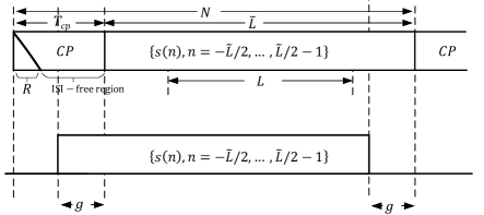
Figure 2: Illustration of the truncation process and relative delay between the transmitted signal and the $\tilde{L}$ samples.

Selecting the ZC sequence as follows:

$$s(n)=e^{j\pi n^{2}/\tilde{L}},n=-\frac{\tilde{L}}{2},-\frac{\tilde{L}}{2}+1,\cdots,\frac{\tilde{L}}{2}-1,$$ (22)

we can add a length-$T_{cp}$ cyclic prefix (CP)

$$\begin{split}&\left[s\left(\frac{\tilde{L}}{2}-T_{cp}\right),s\left(\frac{\tilde{L}}{2}-T_{cp}+1\right),\cdots,s\left(\frac{\tilde{L}}{2}-1\right)\right]\end{split}$$

to transform a $linear$ time delay to a $cyclic$ delay.

While the high-frequency components of the ZC sequence will be affected by the pulse shaping filter, the low-frequency components will be intact. Indeed, it is established in [24, eq. (22)] that the lower-frequency part of the ZC sequence pulse shaped by a raised cosine filter can be represented as a continuous-time chirp signal $x(t)=e^{j\pi t^{2}/\tilde{L}}$ for $-\frac{L}{2}\leq t<\frac{L}{2}$, which has the ambiguity between time-delay and frequency-offset:

$$x(t-\tau)=e^{j\frac{\pi\tau^{2}}{\tilde{L}}}e^{-j\frac{2\pi\tau t}{\tilde{L}}}x(t),\;-\frac{L}{2}\leq t<\frac{L}{2};$$ (23)

that is, a time delay $\tau$ amounts to a frequency offset $\frac{\tau}{\tilde{L}}$.

Denoting

$${\bf x}(\tau)\triangleq\begin{bmatrix}x(-\frac{L}{2}-\tau)\\ x(-\frac{L}{2}+1-\tau)\\ \vdots\\ x(\frac{L}{2}-1-\tau)\end{bmatrix},\;{\bf s}\triangleq\begin{bmatrix}s(-\frac{L}{2})\\ s(-\frac{L}{2}+1)\\ \vdots\\ s(\frac{L}{2}-1)\end{bmatrix},$$ (24)

and recognizing that ${\bf x}(0)={\bf s}$, we can rewrite (23) in the vector form as

$${\bf x}(\tau)=e^{j\frac{\pi\tau^{2}}{\tilde{L}}}{\bf s}\odot{\bf d}\left(-\frac{\tau}{\tilde{L}}\right),$$ (25)

where ${\bf d}(\cdot)$ is as defined in (14).

To have the time-frequency transformation relationship (23) hold, we partially remove the CP, making sure ${\bf y}(0)$ is sampled in the “ISI-free region” (illustrated in Fig. 2). That is, the delayed version of the transmitted signal should be sampled from the “ISI-free region”, otherwise it may suffer from interferences outside of the sequence. In Fig. 2, ${\bf y}(0)$ is sampled $g$-sample ahead the time of $s(0)$, where $T_{cp}-R>g\geq 0$ with the assumption that all the propagation delays are smaller than $R$, which is known a prior. Although the pilot is of length $N=\tilde{L}+T_{cp}$ samples, we only truncate out $\tilde{L}$ samples, indexed from $-\tilde{L}/2$ to $\tilde{L}/2-1$, starting from the ISI-free region as shown in Fig. 2, out of which we further truncate out the low frequency part of the $L$ samples indexed from $-L/2$ to $L/2-1$ for channel estimation. Note again that $L<\tilde{L}$ is chosen to ensure that the ZC sequence filtered by a raised cosine filter is a chirp signal that satisfy (23).

Inserting (25) into (II-B), yields

$$\{\hat{\mbox{\boldmath$\beta$\unboldmath}},\hat{\mbox{\boldmath$\tau$\unboldmath}},\hat{\mbox{\boldmath$\xi$\unboldmath}},\hat{{\mbox{\boldmath$\theta$\unboldmath}}},\hat{\mbox{\boldmath$\varphi$\unboldmath}},\hat{\mbox{\boldmath$\alpha$\unboldmath}},\hat{\overline{\mbox{\boldmath$\tau$\unboldmath}}},\hat{\overline{\mbox{\boldmath$\xi$\unboldmath}}},\hat{\overline{{\mbox{\boldmath$\theta$\unboldmath}}}}\}=\arg\min_{\mbox{\boldmath$\beta$\unboldmath},\mbox{\boldmath$\tau$\unboldmath},\mbox{\boldmath$\xi$\unboldmath},{\mbox{\boldmath$\theta$\unboldmath}},\mbox{\boldmath$\varphi$\unboldmath},\mbox{\boldmath$\alpha$\unboldmath},\overline{\mbox{\boldmath$\tau$\unboldmath}},\overline{\mbox{\boldmath$\xi$\unboldmath}},\overline{{\mbox{\boldmath$\theta$\unboldmath}}}}$$

$$\Arrowvert{\bf Y}-\sum_{u=1}^{U}{\cal W}(\xi_{u}){\bf a}(\theta_{u},\varphi_{u})\beta_{u}e^{j\frac{\pi\tau_{u}^{2}}{\tilde{L}}}{\bf d}\left(\xi_{u}-\frac{\tau_{u}}{\tilde{L}}\right)^{T}\mathop{\rm diag}({\bf s})$$

$$-\sum_{d=1}^{D}{\cal B}(\overline{\xi}_{d}){\bf c}(\overline{\theta}_{d})\alpha_{d}e^{j\frac{\pi\overline{\tau}_{d}^{2}}{\tilde{L}}}{\bf d}\left(\overline{\xi}_{d}-\frac{\overline{\tau}_{d}}{\tilde{L}}\right)^{T}\mathop{\rm diag}({\bf s})\Arrowvert^{2}_{F}.$$ (26)

Denote

$$\tilde{\beta}_{u}\triangleq\beta_{u}e^{\frac{j\pi\tau_{u}^{2}}{\tilde{L}}},\;\tilde{\alpha}_{d}\triangleq\alpha_{d}e^{\frac{j\pi\overline{\tau}_{d}^{2}}{\tilde{L}}}$$ (27)

and

$$\zeta_{u}\triangleq\xi_{u}-\frac{\tau_{u}}{\tilde{L}},\;\overline{\zeta}_{d}\triangleq\overline{\xi}_{d}-\frac{\overline{\tau}_{d}}{\tilde{L}}.$$ (28)

Then (II-B) can be expressed as

$$\{\hat{\tilde{\mbox{\boldmath$\beta$\unboldmath}}},\hat{\mbox{\boldmath$\zeta$\unboldmath}},\hat{\mbox{\boldmath$\xi$\unboldmath}},\hat{{\mbox{\boldmath$\theta$\unboldmath}}},\hat{\mbox{\boldmath$\varphi$\unboldmath}},\hat{\tilde{\mbox{\boldmath$\alpha$\unboldmath}}},\hat{\overline{\mbox{\boldmath$\zeta$\unboldmath}}},\hat{\overline{\mbox{\boldmath$\xi$\unboldmath}}},\hat{\overline{{\mbox{\boldmath$\theta$\unboldmath}}}}\}=\arg\min_{\tilde{\mbox{\boldmath$\beta$\unboldmath}},\mbox{\boldmath$\zeta$\unboldmath},\mbox{\boldmath$\xi$\unboldmath},{\mbox{\boldmath$\theta$\unboldmath}},\mbox{\boldmath$\varphi$\unboldmath},\tilde{\mbox{\boldmath$\alpha$\unboldmath}},\overline{\mbox{\boldmath$\zeta$\unboldmath}},\overline{\mbox{\boldmath$\xi$\unboldmath}},\overline{{\mbox{\boldmath$\theta$\unboldmath}}}}$$

$$\Arrowvert{\bf Y}-\sum_{u=1}^{U}{\cal W}(\xi_{u}){\bf a}(\theta_{u},\varphi_{u})\tilde{\beta}_{u}{\bf d}(\zeta_{u})^{T}\mathop{\rm diag}({\bf s})$$

$$-\sum_{d=1}^{D}{\cal B}(\overline{\xi}_{d}){\bf c}(\overline{\theta}_{d})\tilde{\alpha}_{d}{\bf d}(\overline{\zeta}_{d})^{T}\mathop{\rm diag}({\bf s})\Arrowvert^{2}_{F}.$$ (29)

Denote

$$\tilde{{\bf Y}}\triangleq{\bf Y}\mathop{\rm diag}({\bf s}^{*}),\;{\rm and}\;\tilde{{\bf Y}}=[\tilde{{\bf Y}}_{1}^{T},\cdots,\tilde{{\bf Y}}_{K}^{T}]^{T},$$ (30)

then we can rewrite (II-B) to be

$$\{\hat{\tilde{\mbox{\boldmath$\beta$\unboldmath}}},\hat{\mbox{\boldmath$\zeta$\unboldmath}},\hat{\mbox{\boldmath$\xi$\unboldmath}},\hat{{\mbox{\boldmath$\theta$\unboldmath}}},\hat{\mbox{\boldmath$\varphi$\unboldmath}},\hat{\tilde{\mbox{\boldmath$\alpha$\unboldmath}}},\hat{\overline{\mbox{\boldmath$\zeta$\unboldmath}}},\hat{\overline{\mbox{\boldmath$\xi$\unboldmath}}},\hat{\overline{{\mbox{\boldmath$\theta$\unboldmath}}}}\}=\arg\min_{\tilde{\mbox{\boldmath$\beta$\unboldmath}},\mbox{\boldmath$\zeta$\unboldmath},\mbox{\boldmath$\xi$\unboldmath},{\mbox{\boldmath$\theta$\unboldmath}},\mbox{\boldmath$\varphi$\unboldmath},\tilde{\mbox{\boldmath$\alpha$\unboldmath}},\overline{\mbox{\boldmath$\zeta$\unboldmath}},\overline{\mbox{\boldmath$\xi$\unboldmath}},\overline{{\mbox{\boldmath$\theta$\unboldmath}}}}$$

$$\Arrowvert\tilde{{\bf Y}}-\sum_{u=1}^{U}{\cal W}(\xi_{u}){\bf a}(\theta_{u},\varphi_{u})\tilde{\beta}_{u}{\bf d}(\zeta_{u})^{T}$$

$$-\sum_{d=1}^{D}{\cal B}(\overline{\xi}_{d}){\bf c}(\overline{\theta}_{d})\tilde{\alpha}_{d}{\bf d}(\overline{\zeta}_{d})^{T}\Arrowvert^{2}_{F}.$$ (31)

The next two sections are dedicated to solve this high-dimensional nonlinear problem, first without the direct link between the UE and the BS and then with the link. After solving (II-B), we have from (28) the time delays as

$$\hat{\tau}_{u}=(\hat{\xi}_{u}-\hat{\zeta}_{u})\tilde{L},\;\hat{\overline{\tau}}_{d}=(\hat{\overline{\xi}}_{d}-\hat{\overline{\zeta}}_{d})\tilde{L}$$

$$u=1,\cdots,U,d=1,\cdots,D.$$ (32)

III Estimation of the RIS Channel Without the UE-to-BS Direct Link

In this section, we study the channel estimation problem in the scenario where the direct link between the UE and the BS is blocked. The math derivations in this simpler case will lay foundation for the channel estimation algorithm developed in Section IV for the more general case with the direct link.

Assuming no direct link between the UE and the BS, we can rewrite (II-A) as

$${\bf y}(n)={\bf G}{\bf D}\sum_{u=1}^{U}\beta_{u}{\bf a}(\theta_{u},\varphi_{u})x(n-\tau_{u})e^{j2\pi\xi_{u}n}+{\bf z}(n),$$ (33)

and (II-B) can be simplified as

$$\{\hat{\tilde{\mbox{\boldmath$\beta$\unboldmath}}},\hat{\mbox{\boldmath$\zeta$\unboldmath}},\hat{\mbox{\boldmath$\xi$\unboldmath}},\hat{{\mbox{\boldmath$\theta$\unboldmath}}},\hat{\mbox{\boldmath$\varphi$\unboldmath}}\}=\arg\min_{\tilde{\mbox{\boldmath$\beta$\unboldmath}},\mbox{\boldmath$\zeta$\unboldmath},\mbox{\boldmath$\xi$\unboldmath},{\mbox{\boldmath$\theta$\unboldmath}},\mbox{\boldmath$\varphi$\unboldmath}}$$

$$\left\Arrowvert\tilde{{\bf Y}}-\sum_{u=1}^{U}{\cal W}(\xi_{u}){\bf a}(\theta_{u},\varphi_{u})\tilde{\beta}_{u}{\bf d}(\zeta_{u})^{T}\right\Arrowvert^{2}_{F}.$$ (34)

For ease of presentation, we first address the single path case.

III-A The Channel Estimation in Single-path Case

In the single-path case, we can rewrite (III) to be

$$\begin{split}&\{\hat{\tilde{\beta}},\hat{\zeta},\hat{\xi},\hat{\theta},\hat{\varphi}\}\\ &=\arg\min_{\tilde{\beta},\zeta,\xi,\theta,\varphi}\left\Arrowvert\tilde{{\bf Y}}-\tilde{\beta}{\cal W}(\xi){\bf a}(\theta,\varphi){\bf d}(\zeta)^{T}\right\Arrowvert^{2}_{F}.\end{split}$$ (35)

Expanding (LABEL:eq.ML) to obtain the quadratic function of $\tilde{\beta}$, we can minimize the function with respect to $\tilde{\beta}$ to obtain

$$\tilde{\beta}=\frac{{\bf a}(\theta,\varphi)^{H}{\cal W}(\xi)^{H}\tilde{{\bf Y}}{\bf d}(\zeta)^{*}}{L\times{\bf a}(\theta,\varphi)^{H}{\cal W}(\xi)^{H}{\cal W}(\xi){\bf a}(\theta,\varphi)}.$$ (36)

It follows from (15) that (36) can be rewritten as

$$\tilde{\beta}=\frac{{\bf a}(\theta,\varphi)^{H}{\cal W}(\xi)^{H}\tilde{{\bf Y}}{\bf d}(-\zeta)}{L\times\sum_{k=1}^{K}\left\Arrowvert{\bf a}(\theta,\varphi)^{H}{\bf W}(\Phi_{k})^{H}\right\Arrowvert^{2}}.$$ (37)

Inserting (37) into (LABEL:eq.ML) yields

$$\{\hat{\zeta},\hat{\xi},\hat{\theta},\hat{\varphi}\}=\arg\max_{\zeta,\xi,\theta,\varphi}\frac{\left|{\bf a}(\theta,\varphi)^{H}{\cal W}(\xi)^{H}\tilde{{\bf Y}}{\bf d}(-\zeta)\right|^{2}}{\sum_{k=1}^{K}\left\Arrowvert{\bf a}(\theta,\varphi)^{H}{\bf W}(\Phi_{k})^{H}\right\Arrowvert^{2}}$$ (38)

$$\!=\!\arg\!\max_{\zeta,\xi,\theta,\varphi}\!\!\!\frac{\left|\sum_{k=1}^{K}\!{\bf a}(\theta,\varphi)^{H}{\bf W}(\Phi_{k})^{H}\tilde{{\bf Y}}_{k}{\bf d}(-\zeta)e^{-j2\pi N\xi(k-1)}\right|^{2}}{\sum_{k=1}^{K}\left\Arrowvert{\bf a}(\theta,\varphi)^{H}{\bf W}(\Phi_{k})^{H}\right\Arrowvert^{2}},$$ (39)

which can be coarsely solved using FFTs as explained in the following.

III-A1 Coarse Solution to (39) Using FFTs

The denominator of (39) can be rewritten as

$${\sum_{k=1}^{K}\sum_{m=1}^{M_{r}}\left|{\bf a}(\theta,\varphi)^{H}{\bf w}_{m}^{(k)}\right|^{2}},$$ (40)

where ${\bf w}_{m}^{(k)}$ is the $m$th column of ${\bf W}(\Phi_{k})^{H}$. We can get

$$\begin{split}&{\bf a}(\theta,\varphi)^{H}{\bf w}_{m}^{(k)}\\ &=\sum\limits_{p=1}^{P}\sum\limits_{q=1}^{Q}w_{q,p,m}^{(k)}e^{j\frac{2\pi}{\lambda}(q-1)d_{x}\sin\varphi\cos\theta-j\frac{2\pi}{\lambda}(p-1)d_{z}\cos\varphi},\end{split}$$ (41)

which can be evaluated by applying 2D-FFT to ${\bf w}_{m}^{(k)}$, and $w_{q,p,m}^{(k)}$ is the $((p-1)Q+q)$th element of ${\bf w}_{m}^{(k)}$; thus, (40) can be evaluated efficiently over the mesh grids $-\frac{d_{x}}{\lambda}\sin\varphi\cos\theta=0,\frac{1}{N_{\theta}},\ldots,\frac{N_{\theta}-1}{N_{\theta}},\frac{d_{z}}{\lambda}\cos\varphi=0,\frac{1}{N_{\varphi}},\ldots,\frac{N_{\varphi}-1}{N_{\varphi}}$ using $N_{\theta}\times N_{\varphi}$-point 2D-FFT $KM_{r}$ times.

Since $\{{\bf W}(\Phi_{k}),k=1,\cdots,K\}$ are prescribed, we can actually compute (40) offline and store in advance

$${\bf R}^{(k)}\!\triangleq\!\begin{bmatrix}\begin{array}[]{c}\vdots\\ {\bf a}(\theta,\varphi)^{H}{\bf w}_{1}^{(k)}\\ \vdots\end{array}\cdots\begin{array}[]{c}\vdots\\ {\bf a}(\theta,\varphi)^{H}{\bf w}_{M_{r}}^{(k)}\\ \vdots\end{array}\end{bmatrix}\!\in{\mathbb{C}}^{N_{\theta}N_{\varphi}\times M_{r}},$$ (42)

where the $N_{\theta}N_{\varphi}$-dimensional columns correspond to the $N_{\theta}\times N_{\varphi}$ points 2D-FFT of the corresponding columns of ${\bf W}(\Phi_{k})^{H}$. Then the denominator of (39) is evaluated and stored in vector $\bm{\gamma}\in{\mathbb{C}}^{N_{\theta}N_{\varphi}}$ whose entries are

$$\gamma_{n}=\sum_{k=1}^{K}\|{\bf R}^{(k)}(n,:)\|^{2},$$ (43)

where ${\bf R}^{(k)}(n,:)$ stands for the $n$th row of ${\bf R}^{(k)}$.

According to the expression ${\bf d}(\xi_{u})$ given in (14), in the numerator of (39) $\tilde{{\bf Y}}_{k}{\bf d}(-\zeta)$ can be evaluated efficiently over the mesh grids $\zeta=0,\frac{1}{N_{\zeta}},\ldots,\frac{N_{\zeta}-1}{N_{\zeta}}$ using $N_{\zeta}$-point FFTs to obtain

$${\bf B}^{(k)}\triangleq\begin{bmatrix}\tilde{{\bf Y}}_{k}{\bf d}(0),\cdots,\tilde{{\bf Y}}_{k}{\bf d}(-\frac{N_{\zeta}-1}{N_{\zeta}})\end{bmatrix}\in{\mathbb{C}}^{M_{r}\times N_{\zeta}}.$$ (44)

Denote

$${\bf Q}^{(k)}\triangleq{\bf R}^{(k)}{\bf B}^{(k)}\in{\mathbb{C}}^{({N_{\theta}N_{\varphi}})\times N_{\zeta}},$$ (45)

which corresponds to the term ${\bf a}(\theta,\varphi)^{H}{\bf W}(\Phi_{k})^{H}\tilde{{\bf Y}}_{k}{\bf d}(-\zeta)$ in the numerator of (39). Thus, we can evaluate the numerator of (39) by applying $N_{\xi}$-point FFTs across the $K$ matrices ${\bf Q}^{(k)}$ to obtain a 3D tensor ${\bf M}\in{\mathbb{C}}^{N_{\theta}N_{\varphi}\times N_{\zeta}\times N_{\xi}}$, i.e.,

$${\bf M}(:,:,n_{\xi})=\sum_{k=1}^{K}{\bf Q}^{(k)}e^{-j2\pi\frac{(n_{\xi}-1)(k-1)}{N_{\xi}}},n_{\xi}=1,2,\ldots,N_{\xi}.$$ (46)

Thus, the numerator of (39) can be evaluated by computing the squared absolute values of every entries of ${\bf M}$, which we refer to as ${\bf N}=|{\bf M}|^{2}$. To evaluate the numerator ${\bf N}$ divided by the denominator $\bm{\gamma}$, we compute an $N_{\theta}N_{\varphi}\times N_{\zeta}\times N_{\xi}$ real-valued matrix $\breve{{\bf A}}$ by

$$\breve{{\bf A}}(n,n_{\zeta},n_{\xi})={\bf N}(n,n_{\zeta},n_{\xi})/\gamma_{n}.$$ (47)

By locating the largest entry of $\breve{{\bf A}}$, whose subscript is denoted by $(n_{\varphi},n_{\theta},n_{\zeta},n_{\xi})$, we calculate

$$f_{x}\triangleq\frac{n_{\varphi}-1}{N_{\varphi}},f_{y}\triangleq\frac{n_{\theta}-1}{N_{\theta}},f_{\zeta}\triangleq\frac{n_{\zeta}-1}{N_{\zeta}},f_{\xi}\triangleq\frac{n_{\xi}-1}{N_{\xi}},$$ (48)

of which all range from 0 to 1. We then take the modulo operation

$$f=\left\{\begin{array}[]{ll}f,&f<0.5\\ f-1,&f\geq 0.5\end{array}\right.$$ (49)

so that the frequencies in (48) range from $-0.5$ to $0.5$. Therefore, the channel parameters can be (coarsely) estimated as

$$\varphi=\arccos\left(\frac{\lambda f_{x}}{d_{z}}\right),\;\theta=\arccos\left(-\frac{\lambda f_{y}}{d_{x}\sin\varphi}\right),$$ (50)

$$\hskip 40.00006pt\zeta=f_{\zeta},\quad\xi=f_{\xi}.$$

The online computation involves (44)(45) and (46), which take $\mathcal{O}(KM_{r}N_{\zeta}\log(N_{\zeta}))$ flops, $\mathcal{O}(KN_{\theta}N_{\varphi}M_{r}N_{\zeta})$ flops, and $\mathcal{O}(N_{\theta}N_{\varphi}N_{\zeta}N_{\xi}\log(N_{\xi}))$, respectively. Hence, the total online computational complexity is $\mathcal{O}(KM_{r}N_{\zeta}\log(N_{\zeta})+KN_{\theta}N_{\varphi}M_{r}N_{\zeta}+N_{\theta}N_{\varphi}N_{\zeta}N_{\xi}\log(N_{\xi}))$ flops, a drastically reduced complexity compared with the simplistic method of computing (39) over $N_{\theta}\times N_{\varphi}\times N_{\zeta}\times N_{\xi}$ mesh grid points, which requires $\mathcal{O}(N_{\theta}N_{\varphi}N_{\zeta}N_{\xi}PQLK)$ flops instead.

We emphasize that all the parameters $(\tau,\xi,\theta,\varphi)$ can be conveniently estimated using the FFTs because of the unique property of ZC sequences – a time-delayed ZC appears like one with a frequency offset.

III-A2 Refined Channel Estimation Using Newton’s Method

Given the coarse parameter estimation, we use Newton’s iterative method for refined estimation of $\zeta,\xi$ and $\theta,\varphi$.

With $\hat{\theta}$ and $\hat{\varphi}$ being fixed, since $\zeta$ and $\xi$ are independent of the denominator of (38), $\zeta$ and $\xi$ can be estimated by

$$\{\hat{\zeta},\hat{\xi}\}=\arg\max_{\zeta,\xi}\left|{\bf a}(\hat{\theta},\hat{\varphi})^{H}{\cal W}(\xi)^{H}\tilde{{\bf Y}}{\bf d}(-\zeta)\right|^{2}.$$ (51)

To estimate $\theta$ and $\varphi$ with $\hat{\zeta}$ and $\hat{\xi}$ being fixed, (38) can be simplified as

$$\{\hat{\theta},\hat{\varphi}\}=\arg\max_{\theta,\varphi}\frac{\left|{\bf a}(\theta,\varphi)^{H}{\bf r}\right|^{2}}{\sum_{k=1}^{K}\left\Arrowvert{\bf a}(\theta,\varphi)^{H}{\bf W}(\Phi_{k})^{H}\right\Arrowvert^{2}},$$ (52)

where

$${\bf r}\triangleq{\cal W}(\hat{\xi})^{H}\tilde{{\bf Y}}{\bf d}(-\hat{\zeta}).$$ (53)

Let $\Lambda_{1},\Lambda_{2}$ denote the objective functions of (51) and (52) respectively, i.e.,

$$\Lambda_{1}(\mbox{\boldmath$\psi$\unboldmath}_{1})\triangleq\left|{\bf a}(\hat{\theta},\hat{\varphi})^{H}{\cal W}(\xi)^{H}\tilde{{\bf Y}}{\bf d}(-\zeta)\right|^{2},$$ (54)

and

$$\Lambda_{2}(\mbox{\boldmath$\psi$\unboldmath}_{2})\triangleq\frac{\left|{\bf a}(\theta,\varphi)^{H}{\bf r}\right|^{2}}{\sum_{k=1}^{K}\left\Arrowvert{\bf a}(\theta,\varphi)^{H}{\bf W}(\Phi_{k})^{H}\right\Arrowvert^{2}},$$ (55)

where $\mbox{\boldmath$\psi$\unboldmath}_{1}\triangleq[\zeta,\xi]^{T}$ and $\mbox{\boldmath$\psi$\unboldmath}_{2}\triangleq[\theta,\varphi]^{T}$.

The derivation of the Hessian matrices and Jacobian vectors

$${\bf H}_{1}=\frac{\partial^{2}\Lambda_{1}}{\partial\mbox{\boldmath$\psi$\unboldmath}_{1}\partial\mbox{\boldmath$\psi$\unboldmath}_{1}^{T}},\;{\bf g}_{1}=\frac{\partial\Lambda_{1}}{\partial\mbox{\boldmath$\psi$\unboldmath}_{1}},$$ (56)

and

$${\bf H}_{2}=\frac{\partial^{2}\Lambda_{2}}{\partial\mbox{\boldmath$\psi$\unboldmath}_{2}\partial\mbox{\boldmath$\psi$\unboldmath}_{2}^{T}},\;{\bf g}_{2}=\frac{\partial\Lambda_{2}}{\partial\mbox{\boldmath$\psi$\unboldmath}_{2}}$$ (57)

are routine and are thus relegated to Appendix A in the supplementary document online https://github.com/csrlab-fudan/ris-chan-est/blob/main/appendices.pdf. We can update the estimation as

$$\mbox{\boldmath$\psi$\unboldmath}_{1}^{(i+1)}=\mbox{\boldmath$\psi$\unboldmath}_{1}^{(i)}-s_{1}{\bf H}_{1}^{-1}{\bf g}_{1},$$ (58)

and

$$\mbox{\boldmath$\psi$\unboldmath}_{2}^{(i+1)}=\mbox{\boldmath$\psi$\unboldmath}_{2}^{(i)}-s_{2}{\bf H}_{2}^{-1}{\bf g}_{2},$$ (59)

where $s_{1},s_{2}$ are the step sizes determined by the backtracking line search method [25] to maximize (54) and (55). Then a few alternations between (54) and (55) are needed to achieve the final convergence.

In summary, the proposed scheme for the channel estimation based on RIS in the single-path scenario consists of two steps: i) to obtain the initial estimates according to (39); ii) to use Newton’s method to search for the optimal estimation of (54) and (55). Fast convergence is guaranteed owing to the good, albeit simple, initialization using the FFTs for the Newton’s method. At the end, the estimate of the complex-valued amplitude $\hat{\tilde{\beta}}$ is obtained by substituting the estimated parameters into (37).

We summarize the RIS channel estimation algorithm for the single-path scenario in Algorithm 1.

Algorithm 1 The RIS Channel Estimation in Single-path

1:Input: the received signal ${\bf Y}$.

2:Obtain coarse solution $\{\hat{\zeta},\hat{\xi},\hat{\theta},\hat{\varphi}\}$ to (39) using FFTs as explained in Section III-A1;

3:Initialize $i=0$, $\mbox{\boldmath$\psi$\unboldmath}_{1}^{(0)}=\{\hat{\zeta},\hat{\xi}\}$ and $\mbox{\boldmath$\psi$\unboldmath}_{2}^{(0)}=\{\hat{\theta},\hat{\varphi}\}$;

4:while both $\mbox{\boldmath$\psi$\unboldmath}_{1}^{(i)}$ and $\mbox{\boldmath$\psi$\unboldmath}_{2}^{(i)}$ are not converged do

5:     Calculate ${\bf H}_{1}$, ${\bf g}_{1}$ according to (56);

6:     Update $\mbox{\boldmath$\psi$\unboldmath}_{1}^{(i+1)}$ according to (58);

7:     Update (58);

8:     Calculate ${\bf H}_{2}$, ${\bf g}_{2}$ according to (57);

9:     Update $\mbox{\boldmath$\psi$\unboldmath}_{2}^{(i+1)}$ according to (59);

10:     $i=i+1$;

11:end while

12:Output: $\{\hat{\zeta},\hat{\xi},\hat{\theta},\hat{\varphi}\}$

III-B Channel Estimation in The Multipath Case

Now we proceed to study the multipath case. The key idea is to use the classic SAGE method [20] to decompose the multipath problem to multiple single-path subproblems, to which the method in the previous section can be applied.

The SAGE consists of two steps : the expectation step (E-step), which calculates

$$\hat{\tilde{{\bf Y}}}_{u}=\tilde{{\bf Y}}-\sum_{\begin{subarray}{c}u^{\prime}=1\\ u^{\prime}\neq u\end{subarray}}^{U}\tilde{{\bf Y}}_{u^{\prime}},$$ (60)

where $\tilde{{\bf Y}}$ is as defined in (30) and

$$\tilde{{\bf Y}}_{u}=\hat{\tilde{\beta}}_{u}{\cal W}(\hat{\xi}_{u}){\bf a}(\hat{\theta}_{u},\hat{\varphi}_{u}){\bf d}(\hat{\zeta}_{u})^{T};$$ (61)

the maximization step (M-step), which calculates

$$\begin{split}&\{\hat{\zeta}_{u},\hat{\xi}_{u},\hat{\theta}_{u},\hat{\varphi}_{u}\}\\ &=\arg\max_{\zeta_{u},\xi_{u},\theta_{u},\varphi_{u}}\frac{\left|{\bf a}(\theta_{u},\varphi_{u})^{H}{\cal W}(\xi_{u})^{H}\hat{\tilde{{\bf Y}}}_{u}{\bf d}(-\zeta_{u})\right|^{2}}{\sum_{k=1}^{K}\left\Arrowvert{\bf a}(\theta_{u},\varphi_{u})^{H}{\bf W}(\Phi_{k})^{H}\right\Arrowvert^{2}},\end{split}$$ (62)

to which the solution is delineated in the previous subsection, and

$$\hat{\tilde{\beta}}_{u}=\frac{{\bf a}(\hat{\theta}_{u},\hat{\varphi}_{u})^{H}{\cal W}(\hat{\xi}_{u})^{H}\hat{\tilde{{\bf Y}}}_{u}{\bf d}(-\hat{\zeta}_{u})}{L\times{\sum_{k=1}^{K}\left\Arrowvert{\bf a}(\hat{\theta}_{u},\hat{\varphi}_{u})^{H}{\bf W}(\Phi_{k})^{H}\right\Arrowvert^{2}}}.$$ (63)

We refer to the consecutive iterations for updating the parameter estimates of all the multipaths for one round as an iteration cycle of the SAGE algorithm.

To initialize the SAGE procedure, we assume the received signal contains only one path and estimate $\{\hat{\zeta}_{1},\hat{\xi}_{1},\hat{\theta}_{1},\hat{\varphi}_{1},\hat{\tilde{\beta}}_{1}\}^{(1)}$ via (LABEL:eq.sageM) and (63), where the superscript denotes the iteration index; thus $\tilde{{\bf Y}}_{1}^{(1)}=\hat{\tilde{\beta}}_{1}{\cal W}(\hat{\xi}_{1}){\bf a}(\hat{\theta}_{1},\hat{\varphi}_{1}){\bf d}(\hat{\zeta}_{1})^{T}$ is obtained. Then we set $\hat{\tilde{{\bf Y}}}_{2}^{(1)}=\tilde{{\bf Y}}-\tilde{{\bf Y}}_{1}^{(1)}$ and estimate $\{\hat{\zeta}_{2},\hat{\xi}_{2},\hat{\theta}_{2},\hat{\varphi}_{2},\hat{\tilde{\beta}}_{2}\}^{(1)}$ via (LABEL:eq.sageM) and (63); thus $\tilde{{\bf Y}}_{2}^{(1)}$ is obtained by (61). Next we set $\hat{\tilde{{\bf Y}}}_{3}^{(1)}=\tilde{{\bf Y}}-\tilde{{\bf Y}}_{1}^{(1)}-\tilde{{\bf Y}}_{2}^{(1)}$ and estimate $\{\hat{\zeta}_{3},\hat{\xi}_{3},\hat{\theta}_{3},\hat{\varphi}_{3},\hat{\tilde{\beta}}_{3}\}^{(1)}$, and so on. This procedure continues until $\{\hat{\zeta}_{U},\hat{\xi}_{U},\hat{\theta}_{U},\hat{\varphi}_{U},\hat{\tilde{\beta}}_{U}\}^{(1)}$ with $\hat{\tilde{{\bf Y}}}_{U}^{(1)}=\tilde{{\bf Y}}-\tilde{{\bf Y}}_{1}^{(1)}-\cdots-\tilde{{\bf Y}}_{U-1}^{(1)}$.

In the second round of iteration, first estimate $\{\hat{\zeta}_{1},\hat{\xi}_{1},\hat{\theta}_{1},\hat{\varphi}_{1},\hat{\tilde{\beta}}_{1}\}^{(2)}$ according to (LABEL:eq.sageM) and (63) with $\hat{\tilde{{\bf Y}}}_{1}^{(2)}=\tilde{{\bf Y}}-\tilde{{\bf Y}}_{2}^{(1)}-\tilde{{\bf Y}}_{3}^{(1)}-\cdots-\tilde{{\bf Y}}_{U}^{(1)}$, and obtain $\tilde{{\bf Y}}_{1}^{(2)}$ by (61). Then estimate $\{\hat{\zeta}_{2},\hat{\xi}_{2},\hat{\theta}_{2},\hat{\varphi}_{2},\hat{\tilde{\beta}}_{2}\}^{(2)}$ according to (LABEL:eq.sageM) and (63) with $\hat{\tilde{{\bf Y}}}_{2}^{(2)}=\tilde{{\bf Y}}-\tilde{{\bf Y}}_{1}^{(2)}-\tilde{{\bf Y}}_{3}^{(1)}-\cdots-\tilde{{\bf Y}}_{U}^{(1)}$, and obtain $\tilde{{\bf Y}}_{2}^{(2)}$ by (61) and so on. Proceed the iterations to update the parameters of each path until convergence. The whole SAGE iteration process is summarized in Algorithm 2.

In the above derivations we assume that the number of multipaths $U$ is known. In practice, it can be estimated using, e.g., the Akaike’s information criterion (AIC) [26].

Algorithm 2 The RIS Channel Estimation in Multipath

1:Input: the number of multipath $U$ and the received signal ${\bf Y}$.

2:Initialize $\tilde{{\bf Y}}={\bf Y}\mathop{\rm diag}({\bf s}^{*}),\tilde{{\bf Y}}_{1}=\tilde{{\bf Y}}_{2}=\cdots=\tilde{{\bf Y}}_{U}=0$;

3:while not converged do

4:     for $u=1:U$ do

5:         Calculate $\hat{\tilde{{\bf Y}}}_{u}$ according to (60);

6:         Calculate $\{\hat{\zeta}_{u},\hat{\xi}_{u},\hat{\theta}_{u},\hat{\varphi}_{u}\}$ according to (LABEL:eq.sageM) using Algorithm 1;

7:         Calculate $\hat{\tilde{\beta}}_{u}$ according to (63);

8:         Calculate $\tilde{{\bf Y}}_{u}$ according to (61);

9:     end for

10:end while

11:Output: $\{\hat{\mbox{\boldmath$\zeta$\unboldmath}},\hat{\mbox{\boldmath$\xi$\unboldmath}},\hat{{\mbox{\boldmath$\theta$\unboldmath}}},\hat{\mbox{\boldmath$\varphi$\unboldmath}},\hat{\tilde{\mbox{\boldmath$\beta$\unboldmath}}}\}$

According to (27) and (II-B), we can get

$$\hat{\beta}_{u}=\hat{\tilde{\beta}}_{u}/e^{\frac{j\pi\hat{\tau}_{u}^{2}}{\tilde{L}}},$$ (64)

and

$$\hat{\tau}_{u}=(\hat{\xi}_{u}-\hat{\zeta}_{u})\tilde{L}.$$ (65)

After obtaining $\hat{\mbox{\boldmath$\tau$\unboldmath}}=[\hat{\tau}_{1},\cdots,\hat{\tau}_{U}]^{T}$ and $\hat{\mbox{\boldmath$\beta$\unboldmath}}=[\hat{\beta}_{1},\cdots,\hat{\beta}_{U}]^{T}$, we obtain the estimated time-domain channel response at time $0$

$$\hat{{\bf H}}^{(0)}=\sum_{u=1}^{U}\hat{\beta}_{u}{\bf a}(\hat{\theta}_{u},\hat{\varphi}_{u})p(\tau-\hat{\tau}_{u}).$$ (66)

Hence the projected time-domain channel after time $T$ is

$$\hat{{\bf H}}^{(T)}=\sum_{u=1}^{U}\hat{\beta}_{u}e^{j2\pi\hat{\xi}_{u}T}{\bf a}(\hat{\theta}_{u},\hat{\varphi}_{u})p(\tau-\hat{\tau}_{u}).$$ (67)

where $p(\tau)$ is the raised cosine filter pulse shaper

$$p(\tau)={\rm sinc}(\tau)\frac{{\rm cos}(\pi\mu\tau)}{1-(2\mu\tau)^{2}},$$ (68)

where we have assumed the Nyquist sampling interval $T_{s}=1$ for notational simplicity and $\mu$ is the roll-off factor.

Note that the channel projection is made possible by the estimation of the Doppler frequency offsets $\hat{\xi}_{u},u=1,\ldots,U$.

The frequency-domain channel response of the estimated channel and the projected channel from UE to RIS can be obtained by applying a $\tilde{L}$-point FFT to (66) or (67).

III-C Cramer Rao Bound

To gauge the effectiveness of the proposed algorithm, we derive the CRB of the channel parameter estimation as follows:

Define all the unknown parameters as $\hbox{$\bf\Omega$}=[\mbox{\boldmath$\tau$\unboldmath},\mbox{\boldmath$\xi$\unboldmath},{\mbox{\boldmath$\theta$\unboldmath}},\mbox{\boldmath$\varphi$\unboldmath},\mbox{\boldmath$\beta$\unboldmath}_{r},\mbox{\boldmath$\beta$\unboldmath}_{i}]\in\mathbb{R}^{6U}$, where $\mbox{\boldmath$\tau$\unboldmath}=[\tau_{1},\cdots,\tau_{U}]^{T}$, $\mbox{\boldmath$\xi$\unboldmath}=[\xi_{1},\cdots,\xi_{U}]^{T}$, ${\mbox{\boldmath$\theta$\unboldmath}}=[\theta_{1},\cdots,\theta_{U}]^{T}$, $\mbox{\boldmath$\varphi$\unboldmath}=[\varphi_{1},\cdots,\varphi_{U}]^{T}$, $\mbox{\boldmath$\beta$\unboldmath}_{r}=[\mathop{\rm Re}\{\beta_{1}\},\cdots,\mathop{\rm Re}\{\beta_{U}\}]^{T}$ and $\mbox{\boldmath$\beta$\unboldmath}_{i}=[\mathop{\rm Im}\{\beta_{1}\},\cdots,\\ \mathop{\rm Im}\{\beta_{U}\}]^{T}$. Denote ${\bf y}\triangleq{\mbox{vec}}({\bf Y})$, where

$${\bf Y}=\sum_{u=1}^{U}{\cal W}(\xi_{u}){\bf a}(\theta_{u},\varphi_{u})\beta_{u}({\bf x}(\tau_{u})\odot{\bf d}(\xi_{u}))^{T}+{\bf Z}.$$ (69)

Since ${\mbox{vec}}({\bf A}{\bf B}{\bf C}^{T})=({\bf C}\otimes{\bf A}){\mbox{vec}}({\bf B})$, we have

$${\bf y}={\bf b}+{\mbox{vec}}({\bf Z})$$

$$=\sum_{u=1}^{U}\beta_{u}\left[{\bf x}(\tau_{u})\odot{\bf d}(\xi_{u})\right]\otimes\left[{\cal W}(\xi_{u}){\bf a}(\theta_{u},\varphi_{u})\right]+{\mbox{vec}}({\bf Z}).$$ (70)

Given that ${\bf Z}$ is white Gaussian noise, ${\bf y}\sim{\cal CN}({\bf b},\sigma^{2}{\bf I})$, the expression of the fisher information matrix (FIM) can be written as

$${\bf F}=\frac{2}{\sigma^{2}}\mathop{\rm Re}\left\{\frac{\partial{\bf b}^{H}}{\partial\hbox{$\bf\Omega$}^{T}}\frac{\partial{\bf b}}{\partial\hbox{$\bf\Omega$}}\right\},$$ (71)

where $\frac{\partial{\bf b}}{\partial\hbox{$\bf\Omega$}}=\left[\frac{\partial{\bf b}}{\partial\mbox{\boldmath$\tau$\unboldmath}},\frac{\partial{\bf b}}{\partial\mbox{\boldmath$\xi$\unboldmath}},\frac{\partial{\bf b}}{\partial{\mbox{\boldmath$\theta$\unboldmath}}},\frac{\partial{\bf b}}{\partial\mbox{\boldmath$\varphi$\unboldmath}},\frac{\partial{\bf b}}{\partial\mbox{\boldmath$\beta$\unboldmath}_{r}},\frac{\partial{\bf b}}{\partial\mbox{\boldmath$\beta$\unboldmath}_{i}}\right]\in\mathbb{C}^{KM_{r}L\times 6U}$.

For $\frac{\partial{\bf b}}{\partial\mbox{\boldmath$\tau$\unboldmath}}=\left[\frac{\partial{\bf b}}{\partial\tau_{1}},\cdots,\frac{\partial{\bf b}}{\partial\tau_{U}}\right]$, we have

$$\frac{\partial{\bf b}}{\partial\tau_{u}}=\beta_{u}\left[\frac{\partial{\bf x}(\tau_{u})}{\partial\tau_{u}}\odot{\bf d}(\xi_{u})\right]\otimes\left[{\cal W}(\xi_{u}){\bf a}(\theta_{u},\varphi_{u})\right].$$ (72)

For $\frac{\partial{\bf b}}{\partial\mbox{\boldmath$\xi$\unboldmath}}=\left[\frac{\partial{\bf b}}{\partial\xi_{1}},\cdots,\frac{\partial{\bf b}}{\partial\xi_{U}}\right]$, we have

$$\begin{split}&\frac{\partial{\bf b}}{\partial\xi_{u}}=\beta_{u}\left[{\bf x}(\tau_{u})\odot\frac{\partial{\bf d}(\xi_{u})}{\partial\xi_{u}}\right]\otimes\left[{\cal W}(\xi_{u}){\bf a}(\theta_{u},\varphi_{u})\right]\\ &+\beta_{u}\left[{\bf x}(\tau_{u})\odot{\bf d}(\xi_{u})\right]\otimes\left[\frac{\partial{\cal W}(\xi_{u})}{\partial\xi_{u}}{\bf a}(\theta_{u},\varphi_{u})\right].\end{split}$$ (73)

For $\frac{\partial{\bf b}}{\partial{\mbox{\boldmath$\theta$\unboldmath}}}=\left[\frac{\partial{\bf b}}{\partial\theta_{1}},\cdots,\frac{\partial{\bf b}}{\partial\theta_{U}}\right]$, we have

$$\frac{\partial{\bf b}}{\partial\theta_{u}}=\beta_{u}\left[{\bf x}(\tau_{u})\odot{\bf d}(\xi_{u})\right]\otimes\left[{\cal W}(\xi_{u})\frac{\partial{\bf a}(\theta_{u},\varphi_{u})}{\partial\theta_{u}}\right].$$ (74)

For $\frac{\partial{\bf b}}{\partial\mbox{\boldmath$\varphi$\unboldmath}}=\left[\frac{\partial{\bf b}}{\partial\varphi_{1}},\cdots,\frac{\partial{\bf b}}{\partial\varphi_{U}}\right]$, we have

$$\frac{\partial{\bf b}}{\partial\varphi_{u}}=\beta_{u}\left[{\bf x}(\tau_{u})\odot{\bf d}(\xi_{u})\right]\otimes\left[{\cal W}(\xi_{u})\frac{\partial{\bf a}(\theta_{u},\varphi_{u})}{\partial\varphi_{u}}\right].$$ (75)

For $\frac{\partial{\bf b}}{\partial\mbox{\boldmath$\beta$\unboldmath}_{r}}=\left[\frac{\partial{\bf b}}{\partial\mathop{\rm Re}\{\beta_{1}\}},\cdots,\frac{\partial{\bf b}}{\partial\mathop{\rm Re}\{\beta_{U}\}}\right]$, we have

$$\frac{\partial{\bf b}}{\partial\mathop{\rm Re}\{\beta_{u}\}}=\left[{\bf x}(\tau_{u})\odot{\bf d}(\xi_{u})\right]\otimes\left[{\cal W}(\xi_{u}){\bf a}(\theta_{u},\varphi_{u})\right].$$ (76)

Similarly, $\frac{\partial{\bf b}}{\partial\mbox{\boldmath$\beta$\unboldmath}_{i}}=\sqrt{-1}\frac{\partial{\bf b}}{\partial\mbox{\boldmath$\beta$\unboldmath}_{r}}$.

Based on the above derivations, we insert $\frac{\partial{\bf b}}{\partial\hbox{$\bf\Omega$}}$ into (71). The CRBs of $\left\{\tau_{u},\xi_{u},\theta_{u},\varphi_{u}\right\}$ are given by

$${\rm CRB}(\tau_{u})=[{\bf F}^{-1}]_{u,u},$$ (77)

$${\rm CRB}(\xi_{u})=[{\bf F}^{-1}]_{U+u,U+u},$$ (78)

$${\rm CRB}(\theta_{u})=[{\bf F}^{-1}]_{2U+u,2U+u},$$ (79)

$${\rm CRB}(\varphi_{u})=[{\bf F}^{-1}]_{3U+u,3U+u}.$$ (80)

$${\rm CRB}(\mathop{\rm Re}{(\beta_{u})})=[{\bf F}^{-1}]_{4U+u,4U+u},$$ (81)

and

$${\rm CRB}(\mathop{\rm Im}{(\beta_{u})})=[{\bf F}^{-1}]_{5U+u,5U+u}.$$ (82)

IV Estimation of the RIS Channel With the Direct Link

This section addresses the more general RIS channel estimation problem in the presence of direct path between the BS and the UE. Using the RIS property that the RIS can independently reflect the incident signal by controlling the reflection amplitude [27], we propose to estimate the channel by two steps: i) to shut down the RIS, and estimate ${\bf H}_{d}$ in a way similar to that given in Section III; ii) to turn on the RIS, and we can get the received signal of the reflected path after subtracting the received signal of the direct link, since ${\bf H}_{d}$ has been estimated from the first step.

IV-A The Channel Estimation of ${\bf H}_{d}$

With the RIS being shut down, the user-to-BS channel is a $D$-tap ISI channel, in which the BS receives

$${\bf y}(n)=\sum_{d=1}^{D}\alpha_{d}{\bf c}(\overline{\theta}_{d})x(n-\overline{\tau}_{d})e^{j2\pi\overline{\xi}_{d}n}+{\bf z}(n).$$ (83)

Similar to (II-B), the channel parameters can be estimated as

$$\{\hat{\tilde{\mbox{\boldmath$\alpha$\unboldmath}}},\hat{\overline{\mbox{\boldmath$\zeta$\unboldmath}}},\hat{\overline{\mbox{\boldmath$\xi$\unboldmath}}},\hat{\overline{{\mbox{\boldmath$\theta$\unboldmath}}}}\}\!=\!\arg\!\min_{\tilde{\mbox{\boldmath$\alpha$\unboldmath}},\overline{\mbox{\boldmath$\zeta$\unboldmath}},\overline{\mbox{\boldmath$\xi$\unboldmath}},\overline{{\mbox{\boldmath$\theta$\unboldmath}}}}\!\left\Arrowvert\tilde{{\bf Y}}-\sum_{d=1}^{D}{\cal\overline{B}}(\overline{\xi}_{d}){\bf c}(\overline{\theta}_{d})\tilde{\alpha}_{d}{\bf d}(\overline{\zeta}_{d})^{T}\right\Arrowvert^{2}_{F},$$ (84)

where

$${\mathcal{\overline{B}}}(\overline{\xi}_{d})\triangleq\begin{bmatrix}{\bf I}_{M_{r}}\\ {\bf I}_{M_{r}}e^{j2\pi\overline{\xi}_{d}N}\\ \vdots\\ {\bf I}_{M_{r}}e^{j2\pi\overline{\xi}_{d}(\overline{K}-1)N}\end{bmatrix}\in{\mathbb{C}}^{\overline{K}M_{r}\times M_{r}}.$$ (85)

$\overline{K}$ is the number of observations made for estimating the user-to-BS channel (in contrast, $K$ is the number of observations made for estimating the user-to-RIS channel). Problem (84) can be similarly solved using the algorithms given in Section III as explained in the next.

In the single-path case, (84) degenerates to be

$$\begin{split}\{\hat{\tilde{\alpha}},\hat{\overline{\zeta}},\hat{\overline{\xi}},\hat{\overline{\theta}}\}=\arg\min_{\tilde{\alpha},\overline{\zeta},\overline{\xi},\overline{\theta}}\left\Arrowvert\tilde{{\bf Y}}-\tilde{\alpha}{\cal{\overline{B}}}(\overline{\xi}){\bf c}(\overline{\theta}){\bf d}(\overline{\zeta})^{T}\right\Arrowvert_{F},\end{split}$$ (86)

where$\tilde{{\bf Y}}={\bf Y}\mathop{\rm diag}({\bf s}^{*})$, ${\bf Y}$ is the received signal of the direct path after $\overline{K}$ observations.

Expanding the cost function of (86) to obtain the quadratic function of $\tilde{\alpha}$, since ${{\bf p}}(\overline{\xi})$, ${\bf d}(\overline{\zeta})$ and ${\bf c}(\overline{\theta})$ all have unit-modulus elements, we can minimize the cost function with respect to $\tilde{\alpha}$ to obtain

$$\tilde{\alpha}=\frac{{\bf c}(\overline{\theta})^{H}{\cal\overline{B}}(\overline{\xi})^{H}\tilde{{{\bf Y}}}{\bf d}(-\overline{\zeta})}{L\overline{K}M_{r}}.$$ (87)

Inserting (87) into (86) yields

$$\{\hat{\overline{\zeta}},\hat{\overline{\xi}},\hat{\overline{\theta}}\}=\arg\max_{\overline{\zeta},\overline{\xi},\overline{\theta}}{\left|{\bf c}(\overline{\theta})^{H}{\cal\overline{B}}(\overline{\xi})^{H}\tilde{{{\bf Y}}}{\bf d}(-\overline{\zeta})\right|}$$

$$=\arg\max_{\overline{\zeta},\overline{\xi},\overline{\theta}}{\left|\sum_{k=1}^{\overline{K}}{\bf c}(\overline{\theta})^{H}\tilde{{{\bf Y}}}_{k}{\bf d}(-\overline{\zeta})e^{-j2\pi N\overline{\xi}(k-1)}\right|},$$ (88)

which can be coarsely solved using FFTs as explained in the following.

IV-A1 Coarse Solution to (IV-A) Using FFTs

According to the expression ${\bf c}(\overline{\theta})$ given in (2), ${\bf c}(\overline{\theta})^{H}\tilde{{\bf Y}}_{k}$ can be evaluated efficiently over the mesh grids $-\frac{\bar{d}_{x}}{\lambda}\cos{\overline{\theta}}=0,\frac{1}{N_{\overline{\theta}}},\ldots,\frac{N_{\overline{\theta}}-1}{N_{\overline{\theta}}}$ using $N_{\overline{\theta}}$-point FFTs to obtain

$${\bf C}^{(k)}\triangleq\begin{bmatrix}\begin{array}[]{c}\vdots\\ {\bf c}(\overline{\theta})^{H}\tilde{{\bf Y}}_{k}\\ \vdots\end{array}\end{bmatrix}\in{\mathbb{C}}^{N_{\overline{\theta}}\times L},$$ (89)

According to the expression ${\bf d}(\cdot)$ given in (14),${\bf C}^{(k)}{\bf d}(-\overline{\zeta})$ can be evaluated efficiently over the mesh grids $\overline{\zeta}=0,\frac{1}{N_{\overline{\zeta}}},\ldots,\frac{N_{\overline{\zeta}}-1}{N_{\overline{\zeta}}}$ using $N_{\overline{\zeta}}$-point FFTs to obtain

$${\bf V}^{(k)}\triangleq\begin{bmatrix}{\bf C}^{(k)}{\bf d}(0),\cdots,{\bf C}^{(k)}{\bf d}(-\frac{N_{\overline{\zeta}}-1}{N_{\overline{\zeta}}})\end{bmatrix}\in{\mathbb{C}}^{N_{\overline{\theta}}\times N_{\overline{\zeta}}}.$$ (90)

Thus, we can evaluate (IV-A) by applying $N_{\overline{\xi}}$-point FFTs across the $\overline{K}$ matrices ${\bf V}^{(k)}$ to obtain a 3D tensor ${\bf P}\in{\mathbb{C}}^{N_{\overline{\theta}}\times N_{\overline{\zeta}}\times N_{\overline{\xi}}}$, i.e.,

$${\bf P}(:,:,n_{\overline{\xi}})=\sum_{k=1}^{\overline{K}}{\bf V}^{(k)}e^{-j2\pi\frac{(n_{\overline{\xi}}-1)(k-1)}{N_{\overline{\xi}}}},n_{\overline{\xi}}=1,2,\ldots,N_{\overline{\xi}}.$$ (91)

Thus, (IV-A) can be evaluated by computing the absolute values of every entries of ${\bf P}$, which we refer to as $|{\bf P}|$. By identifying the indices of the largest entry of $|{\bf P}|$, we obtain the estimation $\hat{\overline{\zeta}},\hat{\overline{\xi}},\hat{\overline{\theta}}$ using the procedure similar to that of (48)-(50).

IV-A2 Refined Channel Estimation

Given the initial estimation, we use Newton’s iterative method for refined estimation of $\overline{\zeta}$, $\overline{\xi}$, and $\overline{\theta}$.

Let $\Lambda_{3}$ denote the squared objective function of (IV-A), i.e.,

$$\Lambda_{3}(\mbox{\boldmath$\psi$\unboldmath}_{3})\triangleq\left\arrowvert{\bf c}(\overline{\theta})^{H}{\cal\overline{B}}(\overline{\xi})^{H}\tilde{{{\bf Y}}}{\bf d}(-\overline{\zeta})\right\arrowvert^{2},$$ (92)

where $\mbox{\boldmath$\psi$\unboldmath}_{3}\triangleq[\overline{\zeta},\overline{\xi},\overline{\theta}]^{T}$. The routine derivations of the Hessian matrix and Jacobian vector

$${\bf H}_{3}=\frac{\partial^{2}\Lambda_{3}}{\partial\mbox{\boldmath$\psi$\unboldmath}_{3}\partial\mbox{\boldmath$\psi$\unboldmath}_{3}^{T}},\;{\bf g}_{3}=\frac{\partial\Lambda_{3}}{\partial\mbox{\boldmath$\psi$\unboldmath}_{3}}$$ (93)

can be found in Appendix B in the supplementary document online https://github.com/csrlab-fudan/ris-chan-est/blob/main/appendices.pdf. we can update the estimation as

$$\mbox{\boldmath$\psi$\unboldmath}_{3}^{(i+1)}=\mbox{\boldmath$\psi$\unboldmath}_{3}^{(i)}-s_{3}{\bf H}_{3}^{-1}{\bf g}_{3},$$ (94)

where $s_{3}$ are the step sizes determined by the backtracking line search method to maximize (92). Then the optimal channel estimation can be obtained by using Newton’s method.

In the multipath case, the key idea to use the SAGE algorithm is similar to subsection III-B. That is, to use the SAGE algorithm to decompose the multipath problem to multiple single-path subproblems.

The SAGE consists of two steps: the expectation step (E-step), which calculates

$$\hat{\tilde{{{\bf Y}}}}_{d}=\tilde{{{\bf Y}}}-\sum_{\begin{subarray}{c}d^{\prime}=1\\ d^{\prime}\neq d\end{subarray}}^{D}\tilde{{{\bf Y}}}_{d^{\prime}},$$ (95)

where $\tilde{{{\bf Y}}}_{d}$ is defined as

$$\tilde{{{\bf Y}}}_{d}=\hat{\tilde{\alpha}}_{d}{\cal\overline{B}}(\hat{\overline{\xi}}_{d}){\bf c}(\hat{\overline{\theta}}_{d}){\bf d}(\hat{\overline{\zeta}}_{d})^{T},$$ (96)

and the maximization step (M-step), which calculates

$$\{\hat{\overline{\zeta}}_{d},\hat{\overline{\xi}}_{d},\hat{\overline{\theta}}_{d}\}\!=\!\arg\!\max_{\overline{\zeta}_{d},\overline{\xi}_{d},\overline{\theta}_{d}}\left|{\bf c}({\overline{\theta}}_{d})^{H}{\cal\overline{B}}({\overline{\xi}}_{d})^{H}\hat{\tilde{{{\bf Y}}}}_{d}{\bf d}(-{\overline{\zeta}}_{d})\right|$$ (97)

and

$$\hat{\tilde{\alpha}}_{d}=\frac{{\bf c}(\hat{\overline{\theta}}_{d})^{H}{\cal\overline{B}}(\hat{\overline{\xi}}_{d})^{H}\hat{\tilde{{{\bf Y}}}}_{d}{\bf d}(-\hat{\overline{\zeta}}_{d})}{LKM_{r}}$$ (98)

through $\hat{\tilde{{\bf Y}}}_{d}$. The solution to (97) is already delineated above. The whole SAGE procedure is summarized in Algorithm 3.

Algorithm 3 Channel Estimation of ${\bf H}_{d}$ in Multipath

1:Input: the number of multipath $D$ and the received signal ${{\bf Y}}$.

2:Initialize $\tilde{{\bf Y}}={{\bf Y}}\mathop{\rm diag}({\bf s}^{*}),\tilde{{\bf Y}}_{1}=\tilde{{\bf Y}}_{2}=\cdots=\tilde{{\bf Y}}_{D}=0$;

3:while not converged do

4:     for $d=1:D$ do

5:         Calculate $\hat{\tilde{{\bf Y}}}_{d}$ according to (95);

6:         Calculate $\{\hat{\overline{\zeta}}_{d},\hat{\overline{\xi}}_{d},\hat{\overline{\theta}}_{d}\}$ according to (97);

7:         Calculate $\hat{\tilde{\alpha}}_{d}$ according to (98)

8:         Calculate $\tilde{{\bf Y}}_{d}$ according to (96);

9:     end for

10:end while

11:Output: $\{\hat{\overline{\mbox{\boldmath$\zeta$\unboldmath}}},\hat{\overline{\mbox{\boldmath$\xi$\unboldmath}}},\hat{\overline{{\mbox{\boldmath$\theta$\unboldmath}}}},\hat{\tilde{\mbox{\boldmath$\alpha$\unboldmath}}}\}$

According to (27) and (II-B), we can get

$$\hat{\alpha}_{d}=\hat{\tilde{\alpha}}_{d}/e^{\frac{j\pi\hat{\overline{\tau}}_{d}^{2}}{\tilde{L}}},\;\;\hat{\overline{\tau}}_{d}=(\hat{\overline{\xi}}_{d}-\hat{\overline{\zeta}}_{d})\tilde{L},\;d=1,\ldots,D.$$ (99)

Then the estimated time-domain channel response from the UE to the BS is at time $0$ is

$$\hat{{\bf H}}_{d}^{(0)}=\sum_{d=1}^{D}\hat{\alpha}_{d}e^{j2\pi\hat{\overline{\xi}}_{d}\overline{K}N}{\bf c}(\hat{\overline{\theta}}_{d})p(\tau-\hat{\overline{\tau}}_{d}),$$ (100)

and the projected time-domain channel response from the UE to the BS at time $T$ is

$$\hat{{\bf H}}_{d}^{(T)}=\sum_{d=1}^{D}\hat{\alpha}_{d}e^{j2\pi\hat{\overline{\xi}}_{d}(T+\overline{K}N)}{\bf c}(\hat{\overline{\theta}}_{d})p(\tau-\hat{\overline{\tau}}_{d}).$$ (101)

The corresponding frequency-domain channel response can be obtained by applying an $\tilde{L}$-point FFT to (100) or (101).

IV-B Estimation of the UE-to-RIS Channel

Given the estimation of the parameters of the UE-to-BS direct-link channel $\hat{\overline{\mbox{\boldmath$\zeta$\unboldmath}}},\hat{\overline{\mbox{\boldmath$\xi$\unboldmath}}},\hat{\overline{{\mbox{\boldmath$\theta$\unboldmath}}}},\hat{\tilde{\mbox{\boldmath$\alpha$\unboldmath}}}$, the channel information of the direct link after $\bar{K}$ observations can be obtained as follows

$$\tilde{\breve{{\bf Y}}}=\sum_{d=1}^{D}\hat{\tilde{\alpha}}_{d}e^{j2\pi\hat{\overline{\xi}}_{d}\overline{K}N}{\cal B}(\hat{\overline{\xi}}_{d}){\bf c}(\hat{\overline{\theta}}_{d}){\bf d}(\hat{\overline{\zeta}}_{d})^{T},$$ (102)

where ${\cal B}(\cdot)$ is as defined in (16).

The SAGE consists of two steps : the expectation step (E-step), which calculates

$$\hat{\tilde{{\bf Y}}}_{u}=\tilde{{\bf Y}}-\tilde{\breve{{\bf Y}}}-\sum_{\begin{subarray}{c}u^{\prime}=1\\ u^{\prime}\neq u\end{subarray}}^{U}\tilde{{\bf Y}}_{u^{\prime}},$$ (103)

and $\tilde{{\bf Y}}_{u}$ is defined in (61); the maximization step (M-step), which calculates (LABEL:eq.sageM) and (63) through $\hat{\tilde{{\bf Y}}}_{u}$. The whole SAGE iteration process is summarized in Algorithm 4.

Algorithm 4 Estimation of the RIS Channel With the Direct Link ${\bf H}_{d}$ in Multipath

1:Input: the number of multipath $D$, $U$ and the received signal.

2:Estimate $\{\hat{\overline{\mbox{\boldmath$\zeta$\unboldmath}}},\hat{\overline{\mbox{\boldmath$\xi$\unboldmath}}},\hat{\overline{{\mbox{\boldmath$\theta$\unboldmath}}}},\hat{\tilde{\mbox{\boldmath$\alpha$\unboldmath}}}\}$ using Algorithm 3;

3:Restruct $\tilde{\breve{{\bf Y}}}$ via (102);

4:Initialize $\tilde{{\bf Y}}={\bf Y}\mathop{\rm diag}({\bf s}^{*}),\tilde{{\bf Y}}_{1}=\tilde{{\bf Y}}_{2}=\cdots=\tilde{{\bf Y}}_{U}=0$;

5:while not converged do

6:     for $u=1:U$ do

7:         Calculate $\hat{\tilde{{\bf Y}}}_{u}$ according to (103);

8:         Calculate $\{\hat{\zeta}_{u},\hat{\xi}_{u},\hat{\theta}_{u},\hat{\varphi}_{u}\}$ according to (LABEL:eq.sageM) using Algorithm 1;

9:         Calculate $\hat{\tilde{\beta}}_{u}$ according to (63);

10:         Calculate $\tilde{{\bf Y}}_{u}$ according to (61);

11:     end for

12:end while

13:Output: $\{\hat{\overline{\mbox{\boldmath$\zeta$\unboldmath}}},\hat{\overline{\mbox{\boldmath$\xi$\unboldmath}}},\hat{\overline{{\mbox{\boldmath$\theta$\unboldmath}}}},\hat{\tilde{\mbox{\boldmath$\alpha$\unboldmath}}},\hat{\mbox{\boldmath$\zeta$\unboldmath}},\hat{\mbox{\boldmath$\xi$\unboldmath}},\hat{{\mbox{\boldmath$\theta$\unboldmath}}},\hat{\mbox{\boldmath$\varphi$\unboldmath}},\hat{\tilde{\mbox{\boldmath$\beta$\unboldmath}}}\}$

Therefore, after the RIS is switched on, at time $n=0$, for example, the estimated and the projected time-domain channel responses from UE to RIS is as defined in (66) and (67). And the frequency-domain channel response can be obtained by applying FFTs to the time domain channels.

V Simulation Results

This section evaluates the performance of the proposed scheme through numerical simulations. Consider a $32\times 32$-element RIS (i.e., $M=PQ=1024$) with half wavelength inter-element spacing, and a BS with $M_{r}=6$ antennas. The transmitted pilot is the ZC sequences of length $\tilde{L}=1024$ with cyclic prefix (CP) of length $T_{cp}=64$. The pulse shaper is a raised cosine filter with the roll-off factor $0.3$. The adjustable phases of the RIS are $\{0,\pi/2,\pi,3\pi/2\}$, and the reflection efficiency of the RIS is 0.5. The carrier frequency $f_{c}=28$GHz and the bandwidth $B=50$MHz. Hence the time-duration of an OFDM symbol is about 20$\mu s$. Out of the $1024$-length training sequence, $L=600$ samples corresponding to the lower frequency will be taken out for channel estimation. The dimensions of the FFTs for solving (39) and (IV-A) are $N_{\theta}=32$, $N_{\varphi}=32$, $N_{\overline{\theta}}=32$, $N_{\zeta}=N_{\overline{\zeta}}=1024$ and $N_{\xi}=N_{\overline{\xi}}=64$. All the following simulation results are based on the average of 100 Monte-Carlo trials.

We first simulate the single-path LOS scenario where the direct UE-to-BS link is blocked. The 2D-DOA $\theta=90^{\circ},\varphi=60^{\circ}$, the Doppler frequency offset $\xi=3\times 10^{-6}/T_{s}$ (or 150Hz). According to the velocity-Doppler frequency offset translation $v=\frac{C\xi}{f_{c}}$, where $C$ is the speed of light, the corresponding moving speed $v\approx 1.6m/s$. The time delay $\tau=0.5T_{s}$, and the channel complex gain $\beta=e^{j\phi}$, where $\phi$ was generated at random. The ZC training sequences are transmitted four times ($K=4$); for each of them the RIS phases are varied at random. Fig. 3 shows the root mean square error (RMSE) estimation of the time delay, the Doppler frequency offset, and the two-dimensional angles versus the SNR. We can see that the RMSE results of the proposed scheme overlap with the CRBs as derived in Section III-C, which verify the effectiveness of the proposed method.

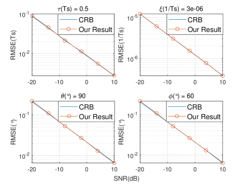
Figure 3: The RMSEs of channel estimation and projection of a single-path case.

In the second example, the simulated channel has six paths with settings: $\mbox{\boldmath$\tau$\unboldmath}=[0.5,1.1,1.8,2.6,5.5,6.4]T_{s}$, $\mbox{\boldmath$\xi$\unboldmath}=[3\times 10^{-4},-10^{-5},10^{-6},10^{-4},3\times 10^{-6},-2\times 10^{-5}]/T_{s}$ (the mobility corresponding to $\xi=3\times 10^{-4}$ is $v\approx 160.7$m/s), ${\mbox{\boldmath$\theta$\unboldmath}}=[40^{\circ},65^{\circ},150^{\circ},100^{\circ},120^{\circ},90^{\circ}]$, $\mbox{\boldmath$\varphi$\unboldmath}=[30^{\circ},50^{\circ},60^{\circ},45^{\circ},40^{\circ},55^{\circ}]$ and the channel gains $[0.85e^{j\phi_{1}},0.8e^{j\phi_{2}},0.7e^{j\phi_{3}},0.65e^{j\phi_{4}},0.6e^{j\phi_{5}},0.5e^{j\phi_{6}}]$, where $\phi_{1},\ldots,\phi_{6}$ are random. The ZC training sequences are transmitted six times ($K=6$), each with a different set of RIS phases. Fig. 4 shows the RMSE of the channel estimation and projection. The RMSE of the channel estimation/projection is calculated by

$${\rm RMSE}=\sqrt{\frac{1}{\tilde{L}M}\|\hat{{\bf H}}-{\bf H}\|_{F}^{2}},$$ (104)

where $\hat{{\bf H}}$ and ${\bf H}$ are the estimated/projected channel and the true channel from the UE to the RIS in the frequency domain, respectively, both with dimensionality $M\times\tilde{L}$. It can be seen from Fig. 4 that the channel projection is quite accurate after 10, 20 and even 40 OFDM symbols.

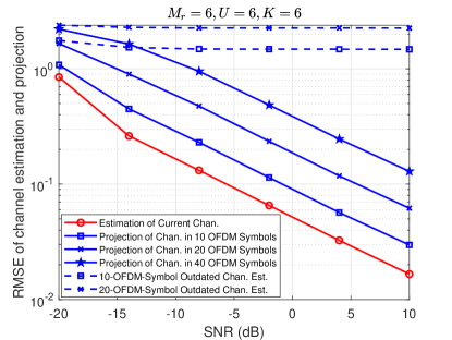
Figure 4: The RMSEs of channel estimation and projection of the UE-to-RIS channel with six paths.

The third example simulates the proposed scheme in the channel with the direct UE-to-BS link, where the channel settings from UE to RIS are the same as those in the second example, $\overline{\mbox{\boldmath$\tau$\unboldmath}}=[0.1,3.5]T_{s}$, $\overline{\mbox{\boldmath$\xi$\unboldmath}}=[6\times 10^{-5},-9\times 10^{-5}]/T_{s}$, $\overline{{\mbox{\boldmath$\theta$\unboldmath}}}=[80^{\circ},110^{\circ}]$, and the channel gains $\mbox{\boldmath$\alpha$\unboldmath}=[e^{j\phi_{7}},0.8e^{j\phi_{8}}]$, where $\phi_{7},\phi_{8}$ are randomly generated. To estimate the direct-link channel, the RIS is turned off at first and the UE transmits the ZC sequences four times ($\bar{K}=4$). Then the RIS is turned on with some random phases and the UE trains the ZC sequences six times ($K=6$). Fig. 5 (a) and Fig. 5 (b) show the RMSEs of the channel estimation and projection of ${\bf H}$ and ${\bf H}_{d}$ under different SNRs respectively. The RMSE of the channel estimation/projection in Fig. 5 (a) is calculated by (104); the RMSE of the channel estimation/projection of the UE-to-BS direct link as shown in Fig. 5 (b) is similarly calculated by

$${\rm RMSE}=\sqrt{\frac{1}{\tilde{L}M_{r}}\|\hat{{\bf H}}_{d}-{\bf H}_{d}\|_{F}^{2}}.$$ (105)

The circled lines in Fig. 5 show the RMSE performance of the channel estimation. The dashed lines represent the RMSE performance of the channel projection without Doppler offset, which show that the channel estimation becomes obsolete quickly after 10 or 20 OFDM symbols. The solid lines marked with squares, crosses and pentagram show that the channel projection enabled by the Doppler estimation can track the time-varying channel quite well after 10, 20 and even 40 OFDM symbols.

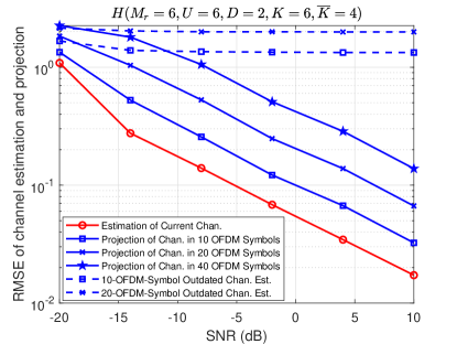
(a) The RMSEs of channel estimation and projection of the UE-to-RIS channel ${\bf H}$

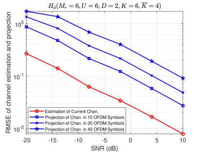
(b) The RMSEs of channel estimation and projection of the UE-to-BS direct-link channel ${\bf H}_{d}$

Figure 5: The RMSEs of channel estimation and projection of a RIS channel with direct link between the UE and the BS.

The last example shows the RMSEs of channel estimation for different number of observations. The channel parameters are set as follows: $\mbox{\boldmath$\tau$\unboldmath}=[0.5,1.1,1.8,2.6]T_{s}$, $\mbox{\boldmath$\xi$\unboldmath}=[3\times 10^{-4},-10^{-5},10^{-6},10^{-4}]/T_{s}$, ${\mbox{\boldmath$\theta$\unboldmath}}=[40^{\circ},65^{\circ},150^{\circ},100^{\circ}]$, $\mbox{\boldmath$\varphi$\unboldmath}=[30^{\circ},50^{\circ},60^{\circ},45^{\circ}]$, and the channel gains $\mbox{\boldmath$\beta$\unboldmath}=[0.85e^{j\phi_{1}},0.8e^{j\phi_{2}},0.7e^{j\phi_{3}},0.6e^{j\phi_{4}}]$, where $\phi_{1},\ldots,\phi_{4}$ are random. The RMSEs of channel estimation of the $U=4$ case versus the number of observations $K=2,3,4,5,6,8,10$ are plotted in Fig. 6, which shows that it requires at least $K=3$ observations to estimate the channel parameters sufficiently well. It is not surprising that the accuracy of channel estimation improves as the number of observations increases.

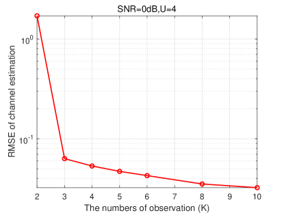
Figure 6: The RMSEs of channel estimation of a $U=4$ case in different $K$.

VI Conclusion

This paper studied uplink channel estimation for an RIS-assisted massive MIMO-OFDM system in a frequency selective channel. By parameterizing the channel in the directions of arrivals (DOA), the time delays, and the frequency offsets, we convert the channel estimation into a parameter estimation problem. We proposed to use the ZC pilot sequences and exploit the time delay-frequency offset ambiguity of the ZC sequences to simplify the high-dimensional parameter estimation problem. The multi-dimensional parameters can be first coarsely initialized via FFTs, before being fine-estimated using Newton’s method. Base on the SAGE method, the multipath parameters estimation problem is transformed into multiple single-path problems. Owing to the estimation of the Doppler frequency offsets, the proposed algorithm can project the time-varying channel, which can greatly reduce the pilot overhead needed for channel estimation, and help mitigate the pilot contamination issue in massive MIMO communications.

References

• [1] Z. Pi and F. Khan, “An introduction to millimeter-wave mobile broadband systems,” IEEE Communications Magazine, vol. 49, no. 6, pp. 101–107, 2011.
• [2] T. S. Rappaport, S. Sun, R. Mayzus, H. Zhao, Y. Azar, K. Wang, G. N. Wong, J. K. Schulz, M. Samimi, and F. Gutierrez, “Millimeter wave mobile communications for 5g cellular: It will work!,” IEEE Access, vol. 1, pp. 335–349, 2013.
• [3] T. E. Bogale and L. B. Le, “Massive MIMO and mmwave for 5G wireless hetnet: Potential benefits and challenges,” IEEE Vehicular Technology Magazine, vol. 11, no. 1, pp. 64–75, 2016.
• [4] T. J. Cui, M. Q. Qi, X. Wan, J. Zhao, and Q. Cheng, “Coding metamaterials, digital metamaterials and programmable metamaterials,” Light-Science & Applications, vol. 3, no. 10, 2014.
• [5] Q. Wu and R. Zhang, “Towards smart and reconfigurable environment: Intelligent reflecting surface aided wireless network,” IEEE Communications Magazine, vol. 58, no. 1, pp. 106–112, 2020.
• [6] N. Shlezinger, G. C. Alexandropoulos, M. F. Imani, Y. C. Eldar, and D. R. Smith, “Dynamic metasurface antennas for 6G extreme massive MIMO communications,” IEEE Wireless Communications, pp. 1–8, 2021.
• [7] M. Nemati, J. Park, and J. Choi, “RIS-assisted coverage enhancement in millimeter-wave cellular networks,” IEEE Access, vol. 8, pp. 188171–188185, 2020.
• [8] K. Venugopal, A. Alkhateeb, N. Gonz lez Prelcic, and R. W. Heath, “Channel estimation for hybrid architecture-based wideband millimeter wave systems,” IEEE Journal on Selected Areas in Communications, vol. 35, no. 9, pp. 1996–2009, 2017.
• [9] F. E. Asim, F. Antreich, C. C. Cavalcante, A. D. Almeida, and J. A. Nossek, “Channel parameter estimation for millimeter-wave cellular systems with hybrid beamforming,” Signal Processing, vol. 176, p. 107715, 2020.
• [10] D. Mishra and H. Johansson, “Channel estimation and low-complexity beamforming design for passive intelligent surface assisted MISO wireless energy transfer,” in ICASSP 2019 - 2019 IEEE International Conference on Acoustics, Speech and Signal Processing (ICASSP), pp. 4659–4663, 2019.
• [11] Z.-Q. He and X. Yuan, “Cascaded channel estimation for large intelligent metasurface assisted massive MIMO,” IEEE Wireless Communications Letters, vol. 9, no. 2, pp. 210–214, 2020.
• [12] Z. Wan, Z. Gao, and M.-S. Alouini, “Broadband channel estimation for intelligent reflecting surface aided mmwave massive MIMO systems,” ICC 2020 - 2020 IEEE International Conference on Communications (ICC), pp. 1–6, 2020.
• [13] B. Zheng and R. Zhang, “Intelligent reflecting surface-enhanced OFDM: Channel estimation and reflection optimization,” IEEE Wireless Communications Letters, vol. 9, no. 4, pp. 518–522, 2020.
• [14] B. Zheng, C. You, and R. Zhang, “Intelligent reflecting surface assisted multi-user OFDMA: Channel estimation and training design,” IEEE Transactions on Wireless Communications, vol. 19, no. 12, pp. 8315–8329, 2020.
• [15] S. Sun and H. Yan, “Channel estimation for reconfigurable intelligent surface-assisted wireless communications considering Doppler effect,” IEEE Wireless Communications Letters, vol. 10, no. 4, pp. 790–794, 2021.
• [16] Z. Mao, M. Peng, and X. Liu, “Channel estimation for reconfigurable intelligent surface assisted wireless communication systems in mobility scenarios,” China Communications, vol. 18, no. 3, pp. 29–38, 2021.
• [17] J. Zhang, C. Qi, P. Li, and P. Lu, “Channel estimation for reconfigurable intelligent surface aided massive MIMO system,” in 2020 IEEE 21st International Workshop on Signal Processing Advances in Wireless Communications (SPAWC), pp. 1–5, 2020.
• [18] O. Elijah, C. Y. Leow, T. A. Rahman, S. Nunoo, and S. Z. Iliya, “A comprehensive survey of pilot contamination in massive MIMO–5G system,” IEEE Communications Surveys Tutorials, vol. 18, no. 2, pp. 905–923, 2016.
• [19] Y. Jiang, B. Daneshrad, and G. J. Pottie, “A practical approach to joint timing, frequency synchronization and channel estimation for concurrent transmissions in a MANET,” IEEE Transactions on Wireless Communications, vol. 16, no. 6, pp. 3461–3475, 2017.
• [20] B. Fleury, M. Tschudin, R. Heddergott, D. Dahlhaus, and K. Ingeman Pedersen, “Channel parameter estimation in mobile radio environments using the SAGE algorithm,” IEEE Journal on Selected Areas in Communications, vol. 17, no. 3, pp. 434–450, 1999.
• [21] D. Su, Y. Jiang, X. Wang, and X. Gao, “Omnidirectional precoding for massive MIMO with uniform rectangular array–part II: Numerical optimization based schemes,” IEEE Transactions on Signal Processing, vol. 67, no. 18, pp. 4772–4781, 2019.
• [22] Z. Gao, C. Hu, L. Dai, and Z. Wang, “Channel estimation for millimeter-wave massive MIMO with hybrid precoding over frequency-selective fading channels,” IEEE Communications Letters, vol. 20, no. 6, pp. 1259–1262, 2016.
• [23] D. Chu, “Polyphase codes with good periodic correlation properties (corresp.),” IEEE Transactions on Information Theory, vol. 18, no. 4, pp. 531–532, 1972.
• [24] Z. Yang, R. Wang, Y. Jiang, and J. Li, “Joint estimation of velocity, angle-of-arrival and range (jevar) using a conjugate pair of zadoff-chu sequences,” IEEE Transactions on Signal Processing, vol. 69, pp. 6009–6022, 2021.
• [25] S. Boyd and L. Vandenberghe, Convex Optimization. 2004.
• [26] H. Akaike, “Information theory and an extension of the maximum likelihood principle,” in 2nd International Symposium on Information Theory, Akademiai Kiado, Budapest (1973), vol. 1, pp. 610–624, 1973.
• [27] H. Yang, X. Chen, F. Yang, S. Xu, X. Cao, M. Li, and J. Gao, “Design of resistor-loaded reflectarray elements for both amplitude and phase control,” IEEE Antennas and Wireless Propagation Letters, vol. 16, pp. 1159–1162, 2017.