Towards a Numerical Proof of Turbulence Closure

Abstract

The development of turbulence closure models, parametrizing the influence of small non-resolved scales on the dynamics of large resolved ones, is an outstanding theoretical challenge with vast applicative relevance. We present a closure, based on deep recurrent neural networks, that quantitatively reproduces, within statistical errors, Eulerian and Lagrangian structure functions and the intermittent statistics of the energy cascade, including those of subgrid fluxes. To achieve high-order statistical accuracy, and thus a stringent statistical test, we employ shell models of turbulence. Our results encourage the development of similar approaches for 3D Navier-Stokes turbulence.

Turbulence is the chaotic and ubiquitous dynamics of fluids, almost unavoidable for high velocity flows. Key to a vast number of environmental and industrial flows [15], 3D turbulence is characterized by a nonlinear forward energy cascade from large scales, where energy is injected, to smaller scales, where it is dissipated via viscous friction [1].

The number of dynamically active degrees of freedom (DOFs) in a turbulent flow is estimated to grow as $Re^{9/4}$ [8], where $Re$ is the Reynolds number, quantifying the turbulent intensity of the flow. Typical natural and industrial flows are characterized by a value of the Reynolds number so high to make it attractive, or even mandatory, the development of so called Large Eddy Simulation (LES) capable of parameterizing, via subgrid closure models, the effect of the smallest scales on the larger ones. However, the complex space-time correlations of turbulence, characterized by intermittent dynamics and anomalous scaling laws [8], challenge physical understanding and hinder the development of accurate and reliable subgrid closure models.

Given the practical importance of turbulence modelling, Large Eddy Simulations have flourished  [14], demonstrating important potential in partially reproducing, in specific geometries, some (statistical) features of the fully resolved Navier-Stokes turbulence.

Due to the fact that turbulence is a (deterministic) chaotic system, the best that any turbulence model could ever achieve is being able to quantitatively reproduce all statistical properties. Additionally, due to intermittency, these statistical properties require in principle the evaluation of arbitrarily high-order space-time statistical moments. Therefore the “perfect” Large Eddy Simulations should be capable of reproducing all statistical moments of the resolved scales, having these indistinguishable from those computed from a filtered direct numerical simulation of the Navier-Stokes equation. Such a demanding requirement has never been accomplished before, making it unclear if this goal could be achieved at all. In this work we show that, within the highest statistical accuracy we could achieve, this task is indeed feasible.

Due to the massive amount of data needed to reach converged statistics of high order statistical moments, we operate in the simplified setting of a reduced dynamical system: the shell model of turbulence [3]. Shell models model the dynamics of homogeneous isotropic turbulence in Fourier space via a (small) number of complex-valued scalars $u_{n}$, $n=0,1,\dots,\infty$, whose magnitude represents the energy of fluctuations at representative logarithmically equispaced spatial scales with wavelength $k_{n}=k_{0}\lambda^{n}$ (usually $\lambda=2$). Shell models reproduce, using a small number of DOFs, the main features of the turbulent energy cascade, including intermittency and anomalous scaling exponents, which are practically indistinguishable from those of real 3D turbulence [13].

The challenge of subgrid closure in the context of the shell model consists in resolving only a subset of the shell variables, $\{u_{n},n=0,\dots,N_{cut}\}$, above an arbitrary subgrid cutoff scale $N_{cut}\ll N_{\eta}$, where $N_{\eta}$ corresponds to the Kolmogorov scale (i.e. $k_{N_{\eta}}$ is the wavelenght of the Kolmogorov scale). This entails modelling the effects of the small scales $\{u_{n},n=N_{cut}+1,\dots,N_{\eta}\}$ on the large scales.

This problem has been recently adressed in [4], where it has been formalized in terms of reduced systems of probability distributions, allowing a precise definition of an optimal subgrid model, although practically intractable, and a series of systematic approximations, yet lacking relevant physical features (correct scaling, energy backscatter). The approach proposed here, which will be denoted as LSTM-LES, employs a custom ODE integrator enhanced by a Long-Short Term Memory (LSTM) [9] Recurrent Neural Network, and is capable of reproducing scaling laws for high order Eulerian (Figure 1) and Lagrangian (Figure 2) structure functions indistinguishable, within statistical accuracy, from those of the fully resolved model, together with intermittency (Figure 3(b)) and energy backscatter (Figure 3(a)), significantly outperforming the state-of-the-art [4].

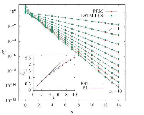
Figure 1: Eulerian structure functions $S_{n}^{p}=\langle|u_{n}|^{p}\rangle$ vs. shell index $n$, in lin-log scale, for orders $p$ from $1$ to $10$ and with $N_{cut}=14$ , comparison between fully resolved model (FRM) and LSTM-LES model. Inset plot: anomalous scaling exponents $\xi_{p}$ of Eulerian structure fuctions, $S_{n}^{p}\propto k_{n}^{-\xi_{p}}$, for the fully resolved model (FRM), the LSTM-LES model, the prediction from Kolmogorov K41 theory [12] and the prediction from She-Leveque model (SL) [16]. For error-bar estimates see supplementary materials.

We consider the SABRA shell model [13], for which the governing equations read:

$$\frac{du_{n}}{dt}=f_{n}+D_{n}+C_{n}=f_{n}\underbrace{-\nu k_{n}^{2}u_{n}}_{D_{n}}+i(ak_{n+1}u_{n+2}u^{*}_{n+1}+bk_{n}u_{n+1}u^{*}_{n-1}+ck_{n-1}u_{n-1}u_{n-2})$$ (1)

with $n=0,1,\dots,N$. For an overview of the parameters, see Table 2. The shell variables $u_{n}$ evolve following three distinct mechanisms, represented by the three terms in the right-hand side of the equation: the forcing ($f_{n}$), injecting energy at large scales, the viscous term ($D_{n}$), dissipating energy at the smaller scales, and the convective term ($C_{n}$), a nonlinear coupling between the shells, responsible for the energy cascade mechanism. The forcing mechanism chosen for our experiments is constant in time, with the magnitude defined by a parameter $\epsilon$, and it is applied only at large scales, with $f_{0}=\epsilon$ and $f_{1}=0.7\epsilon$ (which ensures zero helicity flux [13]), and determines, together with the value of the viscosity $\nu$, the Reynolds number of the model ($Re\sim 1/\nu$).

We now introduce the two models that will be confronted in this paper namely the Fully Resolved Model (FRM), used to generate large amount of data with converged statistics of high-order statistical moments, and our LSTM-LES model, to be trained on the basis of the generated data, and whose target is to reproduce the statistical behavior of the FRM.

The FRM is resolved with a $4^{th}$ order Runge-Kutta scheme with explicit integration of the viscosity [5]. The integration timestep $\Delta t_{GT}$ (for Ground Truth) needs to be sufficiently small as to resolve the complete energy cascade up to the Kolmogorov scale (shell index $N_{\eta}$).

The LSTM-LES model, instead, is composed of the same $4^{th}$ order Runge-Kutta scheme for the evolution of the large scale DOFs $\{u_{n},n=0,\dots,N_{cut}\}$, and a Recurrent Artificial Neural Network, modelling the subgrid closure. The timestep used in this model will be indicated by $\Delta t_{LES}$ and is considerably bigger than $\Delta t_{GT}$ (see Table 2), being $N_{cut}\ll N_{\eta}$ the smallest scale that needs to be explicitly resolved, significantly reducing the computational costs.

Artificial Neural Networks are a class of complex nonlinear models that have been shown to satisfy, under some hypothesis, universal approximation theorems for arbitrary functions [10]. In the last decade they have obtained outstanding results in various fields [11], also comprising fluid dynamics and turbulence modelling [7, 2, 6]. We employ a Recurrent Neural Network (RNN) architecture [17], which is particularly useful in the context of time series data since the input of the neural network is composed by a present input term and by a state (or memory) term, coming from a previous evaluation of the network. In particular, we use Long-Short Term Memory (LSTM) networks, which are a particular istance of recurrent neural networks that implement a gating mechanism in order to alleviate the problem of vanishing/exploding gradients during training [9].

Before explaining the functioning of the LSTM-LES model, described extensively in the supplementary materials, we highlight one of the main assumptions made in the definition of the SABRA shell model. This feature, crucial for our subgrid closure approach, is the locality in Fourier space of the convective term $C_{n}$, mimicking the Richardson energy cascade model [8]. This means that the convective term for the shell with index $n$ depends only on shells indexed by $\{n-2,n-1,n,n+1,n+2\}$ (see Equation 1). This implies that, after performing the subgrid cut at shell $N_{cut}$, the only shells for which $\frac{du_{n}}{dt}$ remains undefined are $n=N_{cut}$ and $n=N_{cut}-1$, and that to compute the value of the derivative for those shells is necessary to model the values of $u_{N_{cut}+1}$ and $u_{N_{cut}+2}$. The subgrid closure modelling, performed by the Neural Network, consists then in the prediction of these two shells given the present and past state of the large scales:

$$\begin{pmatrix}u_{0}(t),\cdots,u_{N_{cut}}(t)\\ state(t)\end{pmatrix}\xmapsto{\text{LSTM}}\begin{pmatrix}u_{N_{cut}+1}(t),u_{N_{cut}+2}(t)\\ state(t+\Delta t_{LES})\end{pmatrix}.$$ (2)

We train our Neural Network in an a-priori fashion by asking for one-step pointwise prediction, without using the predicted value to advance to the next timestep (for more details on the training procedure, see the supplementary material). We opt for this approach because of the chaoticity of turbulence, reproduced by the SABRA shell model [3]. Analogously, we test the network by confronting the LSTM-LES model and the FRM only in terms of statistical quantities such as distributions and statistical moments, avoiding meaningless computation of pointwise errors.

In the following, we present and discuss the performances of the LSTM-LES model in comparison with the fully resolved model (FRM) and the literature [4].

We begin by considering the scaling of the $p^{th}$ order Eulerian structure functions, with $p=1,\cdots,10$ computed as:

$$S_{n}^{p}=\langle|u_{n}|^{p}\rangle.$$ (3)

The results are shown in Figure 1. The LSTM-LES model is indistinguishable, within statistical accuracy, from the fully resolved model. This can be further verified by considering the value of the scaling exponents $\xi_{p}$ ($S_{n}^{p}\propto k_{n}^{-\xi_{p}}$) as a function of the order, $p$, of the structure function, as shown in the inset of Figure 1 and reported in Table Towards a Numerical Proof of Turbulence Closure.

Order	K41	SL	FRM	LSTM-LES
$1$	$0.3333$	$0.3640$	$0.423\pm 0.005$	$0.423\pm 0.005$
$2$	$0.6667$	$0.6959$	$0.78\pm 0.01$	$0.78\pm 0.01$
$3$	$1.0000$	$1.0000$	$1.10\pm 0.02$	$1.10\pm 0.02$
$4$	$1.3333$	$1.2797$	$1.38\pm 0.03$	$1.39\pm 0.02$
$5$	$1.6667$	$1.5380$	$1.64\pm 0.04$	$1.65\pm 0.03$
$6$	$2.0000$	$1.7778$	$1.89\pm 0.06$	$1.89\pm 0.05$
$7$	$2.3333$	$2.0013$	$2.11\pm 0.08$	$2.12\pm 0.07$
$8$	$2.6667$	$2.2105$	$2.33\pm 0.11$	$2.33\pm 0.09$
$9$	$3.0000$	$2.4074$	$2.54\pm 0.14$	$2.53\pm 0.12$
$10$	$3.3333$	$2.5934$	$2.74\pm 0.16$	$2.73\pm 0.15$

Table 1: Anomalous exponents $\xi_{p}$ for the scaling laws of the Eulerian structure fuctions $S_{n}^{p}=\langle|u_{n}|^{p}\rangle\propto k_{n}^{-\xi_{p}}$ for the fully resolved model (FRM), the LSTM-LES model, the prediction from Kolmogorov K41 theory, and the prediction from She-Leveque model (SL). For error-bar estimates see supplementary material.

In order to establish the capability of the LSTM-LES model to reproduce time correlations of the signal, we considered the behavior of the Lagrangian structure functions. These are computed as the time correlation functions of Lagrangian signals obtained by summing the real parts of all the shells $u(t)=\Re(\sum_{n}u_{n}(y))$ [3]:

$$L^{p}_{\tau}=\langle|u(t+\tau)-u(t)|^{p}\rangle.$$ (4)

The results are shown in Figure 2, where we can see that the LSTM-LES model closely follows the scaling laws of the fully resolved model.

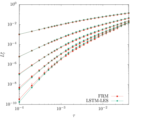
Figure 2: Lagrangian structure functions (see Eq. 4), in log-log scale ($\tau$ on the x-axis, $p=1,..,5$), comparison between the fully resolved model (FRM) and LSTM-LES model. For error-bar estimates see supplementary material.

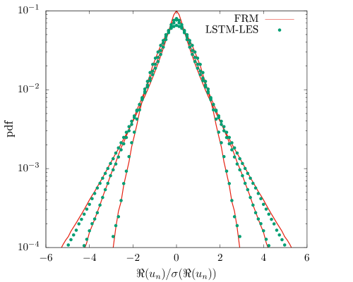
(a)

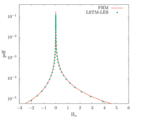
(b)

Figure 3: (a) PDF of the real part of shells 4, 8 and 12, in log scale, normalized with standard deviation $\Re u_{n}/\sigma(\Re u_{n})$ for the fully resolved model (FRM), and the LSTM-LES model. (b) PDF of the convective fluxes (Eq. 5) at shell $n=N_{cut}$, for the fully resolved model (FRM) and the LSTM-LES model.

In terms of statistical distributions, we show, in Figure 3(b), the distributions for the real part of shells 4, 8 and 12 ($N_{cut}=14,N_{\eta}=30$), normalized by standard deviation, $(\Re u^{n})/(\sigma(\Re u^{n}))$. Notably, the model correctly reproduces intermittency at the small scales, characterized by the non-gaussian nature of the pdf.

In order to evaluate the capability of the subgrid closure to properly model the energy fluxes to the unresolved scales, we consider the distribution for the convective fluxes computed at the subgrid cut $N_{cut}$ [4]:

$$\Pi_{N_{cut}}=k_{0}\lambda^{N_{cut}}(\lambda au_{N_{cut}+2}u_{N_{cut}+1}^{*}u_{N_{cut}}^{*}+bu_{N_{cut}+1}u_{N_{cut}}^{*}u_{N_{cut}-1}^{*}).$$ (5)

The results are shown in Figure 3(a), where we can see that the phenomenon of backscatter, i.e. the presence of events of net energy fluxes going from small scales to large scales (negative values of the flux in the plot), is well captured by our model. This behavior is tipically very hard to reproduce in typical LES schemes and, when included improperly, it can even compromise the scheme stability [8].

Finally, we present a comparison of the LSTM-LES model with the three physics-based alternatives proposed in [4], denoted respectively with sm0, sm1 and smk, and corresponding to three different approximation of the optimal subgrid closure scheme. The comparison is made in terms of local slopes for the $2^{nd}$ order Eulerian structure functions, computed as finite differences $\frac{\Delta S^{2}_{n}}{\Delta n}$ (Figure 4). We can see that our model significantly outperforms the three models presented in [4]. In fact, the models sm0 and sm1 present wide oscillations around the correct scaling law $\frac{\Delta S^{2}_{n}}{\Delta n}=-\xi_{2}\approx-0.78$. The model denoted as smk instead, i.e. the one with better scaling properties, does not entail backscatter, which is present (though not perfectly resolved) in sm0, sm1.

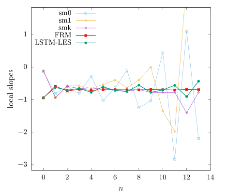
Figure 4: Local slopes for the second order Eulerian structure function $\frac{\Delta S^{2}_{n}}{\Delta n}$ vs. shell index $n$. Comparison between fully resolved model (FRM), LSTM-LES model and three physics based model introduced in [4], denoted as sm0, sm1 and smk.

In this work we have provided a numerical proof of the fact that turbulence closures are possible. Specifically, we have focused on the ambitious goal of developing a model for the small (unresolved) scales capable of reproducing a dynamics of the large (resolved) scales that is statistically indistinguishable from the fully resolved dynamics. Our model, based on a deep learning approach, implements a closure on a shell model of turbulence. While shell models are simplified versions of the Navier-Stokes equation, they are well know for faithfully reproducing the complex phenomenology of the turbulent energy flux, including multiscale correlations and intermittency.

Employing shell models for turbulence allowed us to work in a well-controlled environment where high Reynolds numbers, and thus clean scaling laws over several orders of magnitude, are easily achievable. Additionally, due to the computational lightweight of the shell models, we could perform stringent statistical comparisons, something that would have not been easily achievable in the framework of the full Navier-Stokes equation.

We numerically demonstrated that our subgrid closure model generates a dynamics indistinguishable, in statistical terms, from that of a filtered fully resolved simulation. To this aim, we considered high order Eulerian and Lagrangian structure functions together with distributions of shell variables and convective fluxes. Additionally we showed that our model yields results that outperform the state-of-the-art physics based approaches proposed in literature [4].

Our results provide solid foundations towards the possibility to develop subgrid closure for Navier-Stokes that are capable of faithfully reproducing all statistical properties of 3D turbulence.

1 Supplementary Materials

1.1 LSTM-LES model

We provide here the details about our LSTM-LES deep learning model, implementing the subgrid closure for the SABRA shell model. This is composed by a combination of a $4^{th}$ order Runge Kutta integration scheme with explicit integration of the viscosity [5], together with a LSTM Recurrent Neural Network that provides the value of the fluxes to/from the unresolved scales.

Thanks to the locality of the convective term $C_{n}$ (Eq. 1), we can close (and resolve) the large scale system, denoted here by convenience $u^{<}=\{u^{n},n=0,\cdots,N_{cut}\}$, by only providing the values of the shells below the subgrid cutoff scale, denoted $u^{>}=\{u_{N_{cut}+1},u_{N_{cut}+2}\}$, given as output of a LSTM Neural Network. However, this is only true for one-step schemes such as Explicit Euler. As we employ a $4^{th}$ order Runge Kutta multistepping integration scheme, a dependency on higher shell indexes (up to $u_{N_{cut}+8}$) emerges, since we need more terms to approximate the higher order derivatives in the scheme. Our approach consists then in an application of the LSTM Neural Network for each of the sub-steps of the multistepping scheme.

Specifically, the LSTM-LES model (cf. Figure 5) takes as input the large scales of turbulence, above the subgrid cutoff $N_{cut}$, at time $t$, $u^{<}(t)$, and the hidden state from the previous timestep $h(t)$, and returns $u^{<}(t+\Delta t)$ and the hidden state for the next timestep $h(t+\Delta t)$ (here and in the following we will indicate for conciseness $\Delta t_{LES}$ with $\Delta t$).

In order to compute $u^{<}(t+\Delta t)$, we need to evaluate the four terms $k_{1},k_{2},k_{3}$ and $k_{4}$, and use them to advance the large scales in time, in formulas:

$$u^{<}(t+\Delta t)=u^{<}(t)+\frac{\Delta t}{6}(k_{1}+2k_{2}+2k_{3}+k_{4}).$$ (6)

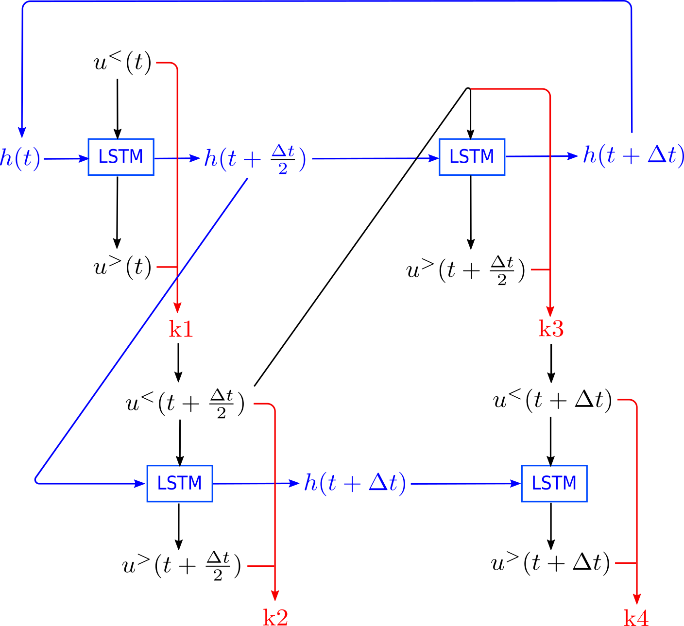
Figure 5: LSTM-LES model. The input of the timestepping scheme are the hidden state $h(t)$ and the value of the solution at the large scales, before the cut, $u^{<}(t)$. The scheme computes the four terms $k1,k2,k3$ and $k4$, and uses those to update $u^{<}(t)$ according to Eq. 6.

The scheme is then composed of 4 steps:

1. (top left of Figure 5) use $u^{<}(t)$ and $h(t)$ (both from the previous timestep) to compute $k_{1}=\frac{du^{<}}{dt}(t)$ and return $h(t+\frac{\Delta t}{2})$. After that, compute $u^{<}(t+\frac{\Delta t}{2})$ using an Exlicit Euler scheme:

   $$u^{<}(t+\frac{\Delta t}{2})=u^{<}(t)+\frac{\Delta t}{2}\frac{du^{<}}{dt}(t);$$ (7)

2. (bottom left) use $u^{<}(t+\frac{\Delta t}{2})$ (computed in 1.) and the hidden state $h(t+\frac{\Delta t}{2})$ (computed in 1.) to compute $k2=\frac{du^{<}}{dt}(t+\frac{\Delta t}{2})$ and $h(t+\Delta t)$;

3. (top right) use $u^{<}(t+\frac{\Delta t}{2})$ (computed in 2.) and $h(t+\frac{\Delta t}{2})$ (computed in 1.) to compute $k3=\frac{du^{<}}{dt}(t+\frac{\Delta t}{2})$, use that to compute $u^{<}(t+\Delta t)$ like in Equation 7, and feed in the output hidden state $h(t+\Delta t)$ for the next timestep;

4. (bottom right) use $u^{<}(t+\Delta t)$ (computed in 3.) and $h(t+\Delta t)$ (computed in 2.) to compute $k4=\frac{du^{<}}{dt}(t+\Delta t)$.

In the scheme above, the LSTM model used (architecture, values of weights/biases) is the same for all the 4 steps. The only differences are in the input, $u^{<}$, and the hidden state, $h$, resulting in different outputs. Moreover, the hidden states are organized to have time consistency of the LSTM, i.e. the input of the LSTM $u^{<}$ and the hidden state $h$ are evaluated at the same timestep, where one evaluation of the LSTM corresponds to half a timestep. Finally, we remark that requiring the time consistency between hidden states and solution does not fully define the scheme, and that we could have reorganized the topology of the graph of Figure 5 in different ways, possibly obtaining different results. From the experiments done, different reorganizations of the topology did not give qualitateively different results; this will be investigated more deeply in a future work.

Parameter	Value	Description
$\nu$	$1\times 10^{-12}$	viscosity
Re	$\approx 10^{12}$	Reynolds number
$\epsilon$	$0.5$	forcing
$N$	$40$	number of shells
$N_{\eta}$	$30$	Kolmogorov scale
$N_{cut}$	$14$	subgrid cutoff scale
$\tau_{0}$	$7.553\times 10^{-1}$	eddy turnover time for the integral scale
$\tau_{\eta}$	$1.8367\times 10^{-6}$	eddy turnover time for the dissipative scale
$\Delta t_{GT}$	$1\times 10^{-8}$	timestep of FRM
$\Delta t_{LES}$	$1\times 10^{-5}$	timestep of LES-LSTM model
$N_{data}$	$5000$	number of initial conditions of dataset
$N_{batch}$	$3000$	batch size for training
$T_{train}$	$20480\times\Delta t_{LES}$	integration time of training dataset
$T_{test}$	$81920\times\Delta t_{LES}$	integration time of test dataset
bptt	$32$	backpropagation through time truncation parameter

Table 2: Values of the parameters of the numerical experiments.

1.2 Model Training and Testing

The ground truth datasets for training of the LSTM is generated by integrating the shell model with the FRM model for a certain number of random initial conditions $N_{data}$ and for a fixed time interval $T_{train}$ (after a transient). The timestep used in this phase is $\Delta t_{GT}$. We dump the solution every $\frac{\Delta t_{GT}}{\Delta t_{LES}}$ timesteps, where $\Delta t_{LES}$ is the timestep of the LSTM-LES model, for a total of $T_{train}$ time snapshots.

The training is then done by considering a batch size of $N_{batch}$ intial conditions, randomly sampled at each epoch from the training set, and by performing Truncated Backpropagation Through Time (TBTT) over it [17].

Specifically, we take the following steps:

$epoch\leftarrow 0$

while $epoch<n\_epochs$ do

     $t\leftarrow 0$

     select randomly $N_{batch}$ ICs from $N_{data}$ $\rightarrow$ $u^{<}(0)$

     while $t<T$ do

         $loss\leftarrow 0$

         for $k=0$; $k<\text{tbtt}$; $k\mathrel{+}=1$  do

              $u^{<}(t+\Delta t_{LES})=\text{LSTM-LES}(u^{<}(t))$

              $t\leftarrow t+\Delta t_{LES}$

              $loss\leftarrow loss+\mathcal{L}(u^{<}(t),u_{GT}^{<}(t))$

         end for

         backpropagate loss through LSTM

         update LSTM parameters via gradient descent

     end while

end while

As a loss function, $\mathcal{L}(u,v)$, we used the classical $L^{2}$ loss $||u-v||^{2}$ applied to shells $N_{cut}-8$ to $N_{cut}$. For the gradient descent we used the Adam optimizer with adaptative learning rate (initial value $lr_{0}=3e-4$).

The testing is done by confronting the FRM model and the LSTM-LES model in terms of statistical quantities (Eulerian and Lagrangian structure functions, distributions, anomalous exponents). These statistics are computed for the two models, respectively:

• (FRM model) by considering the test ground truth dataset, i.e.  $N_{data}$ different initial conditions for $T_{test}$ timesteps. The timestep used in this phase is $\Delta t_{GT}$. We dump the solution every $\frac{\Delta t_{GT}}{\Delta t_{LES}}$ timesteps, where $\Delta t_{LES}$ is the timestep of the LSTM-LES model.

• (LSTM-LES model) by taking the final state of the $N_{data}$ solutions of the test ground truth dataset and integrating forward, using the LSTM-LES model, for the same number of timesteps $T_{test}$ of size $\Delta t_{LES}$.

We estimate the error-bars by splitting the datasets in chunks consisting of $1024$ time snapshots (for a total of $80$ chunks). We then compute individual statistics on these chunks, and report the average of these statistics as a central point, and the difference between minimum and maximum as the error-bar.

References

- [1] A. Alexakis and L. Biferale. Cascades and transitions in turbulent flows. Phys. Rep., 767-769:1–101, 2018.
- [2] A. Beck and M. Kurz. A perspective on machine learning methods in turbulence modeling. GAMM-Mitteilungen, 44, 03 2021.
- [3] L. Biferale. Shell models of energy cascade in turbulence. Annu. Rev. Fluid Mech., 35(1):441–468, 2003.
- [4] L. Biferale, A. A. Mailybaev, and G. Parisi. Optimal subgrid scheme for shell models of turbulence. Phys. Rev. E, 95(4), Apr 2017.
- [5] T. Bohr, M. H. Jensen, G. Paladin, and A. Vulpiani. Dynamical Systems Approach to Turbulence. Cambridge University Press, 1998.
- [6] A. Corbetta, V. Menkovski, R. Benzi, and F. Toschi. Deep learning velocity signals allow quantifying turbulence intensity. Science Advances, 7(12):eaba7281, 2021.
- [7] K. Duraisamy, G. Iaccarino, and H. Xiao. Turbulence modeling in the age of data. Annu. Rev. Fluid Mech., 51(1):357–377, Jan 2019.
- [8] U. Frisch. Turbulence: The Legacy of A. N. Kolmogorov. Cambridge University Press, 1995.
- [9] S. Hochreiter and J. Schmidhuber. Long short-term memory. Neural Comput., 9(8):1735–1780, Nov 1997.
- [10] K. Hornik, M. Stinchcombe, and H. White. Multilayer feedforward networks are universal approximators. Neural Netw., 2(5):359–366, 1989.
- [11] J. Jumper, R. Evans, A. Pritzel, T. Green, M. Figurnov, O. Ronneberger, K. Tunyasuvunakool, R. Bates, A. Žídek, A. Potapenko, A. Bridgland, C. Meyer, S. A. A. Kohl, A. J. Ballard, A. Cowie, B. Romera-Paredes, S. Nikolov, R. Jain, J. Adler, T. Back, S. Petersen, D. Reiman, E. Clancy, M. Zielinski, M. Steinegger, M. Pacholska, T. Berghammer, S. Bodenstein, D. Silver, O. Vinyals, A. W. Senior, K. Kavukcuoglu, P. Kohli, and D. Hassabis. Highly accurate protein structure prediction with alphafold. Nature, 596(7873):583–589, Aug 2021.
- [12] A. N. Kolmogorov. The local structure of turbulence in incompressible viscous fluid for very large reynolds numbers. Proc. Math. Phys. Eng. Sci., 434(1890):9–13, 1991.
- [13] V. S. L’vov, E. Podivilov, A. Pomyalov, I. Procaccia, and D. Vandembroucq. Improved shell model of turbulence. Phys. Rev. E, 58(2):1811–1822, Aug 1998.
- [14] C. Meneveau and J. Katz. Scale-invariance and turbulence models for large-eddy simulation. Annual Review of Fluid Mechanics, 32(1):1–32, 2000.
- [15] S. B. Pope. Turbulent Flows. Cambridge University Press, 2000.
- [16] Z.-S. She and E. Leveque. Universal scaling laws in fully developed turbulence. Phys. Rev. Lett., 72:336–339, Jan 1994.
- [17] A. Sherstinsky. Fundamentals of recurrent neural network (rnn) and long short-term memory (lstm) network. Physica D., 404:132306, 2020.