Optimization of the Sparse Multi-Threaded Cholesky Factorization for A64FX

Abstract.

Sparse linear algebra routines are fundamental building blocks of a large variety of scientific applications. Direct solvers, which are methods for solving linear systems via the factorization of matrices into products of triangular matrices, are commonly used in many contexts. The Cholesky factorization is the fastest direct method for symmetric and definite positive matrices. This paper presents selective nesting, a method to determine the optimal task granularity for the parallel Cholesky factorization based on the structure of sparse matrices. We propose the OPT-D-COST algorithm, which automatically and dynamically applies selective nesting. OPT-D-COST leverages matrix sparsity to drive complex task- based parallel workloads in the context of direct solvers. We run an extensive evaluation campaign considering a heterogeneous set of 60 sparse matrices and a parallel machine featuring the A64FX processor. OPT-D-COST delivers an average performance speedup of 1.46$\times$ with respect to the best state-of-the-art parallel method to run direct solvers.

1. Introduction

Linear algebra routines are common building blocks of scientific computing workloads. In particular, direct linear solvers are widely used. Indeed, a very common way to solve a system such as $Ax=b$ is to factorize matrix $A$ into a product of triangular matrices. When dealing with symmetric and definite positive matrices, the Cholesky factorization ((hornJohnsonMatrix, ), Corollary 7.2.9) is faster than alternative direct methods like the LU ((hornJohnsonMatrix, ), Definition 3.5.1) or the QR ((hornJohnsonMatrix, ), Theorem 2.1.14) factorizations. The Cholesky decomposition factorizes matrix $A$ in terms of a product of a lower triangular matrix $L$ and its transposed matrix $L^{T}$, that is, $A=LL^{T}$.

For the case of sparse matrices, there are several high-performance parallel solvers implementing the Cholesky factorization: MUMPS (mumps, ), PaStiX (pastix, ), PARDISO (PARDISO, ) or CHOLMOD (cholmod, ). CHOLMOD is one of the most widely used implementations of the Cholesky factorization. It is an open source software.In particular, CHOLMOD implements a supernodal version of the Cholesky factorization. Supernodal algorithms rely on a decomposition of the matrix in terms of blocks of columns, that we call supernodes. These algorithms rely on sub-operations (Level-3 BLAS kernels) on a supernode or between supernodes to perform the factorization of the whole matrix. Like many numerical solvers, CHOLMOD is composed of three main computing phases: The first one analyzes the structure of the matrix and reorders matrix rows and columns to minimize the fill-in, i.e. the number of non-zero elements in the final factorization. The second phase factorizes the matrix by applying BLAS kernels within a supernode or between them, and the third one solves a couple of triangular systems of equations, namely $Ly=b$ and $L^{T}x=y$ in the case of Cholesky factorization. Among the three phases, the factorize phase represents the bulk of the CHOLMOD solver.

Although the state-of-the-art CHOLMOD implementation is sequential, one can easily link it with multi-threaded BLAS libraries (BLAS, ) to take advantage of many-core architectures. Other approaches rely on task-level parallelism to run direct solvers on sparse matrices (tangHybrid, ; pastixRuntime, ). They exploit the structure of the elimination tree (liuTree, ), which represents the order in which supernodes have to be factorized, to orchestrate the parallel run. Other aspects of the matrix sparse pattern are usually ignored by previous works. Since the computational load of every task heavily depends on the structure of its corresponding supernode, current schemes are prone to load balancing problems. More advanced approaches (mumpsQR, ), consider different features of the input matrix to optimize the setup of the parallel run in terms of aspects like task granularity, but determining the quality of these parameter setups requires trying them all.

This paper presents selective nesting, a method to determine the optimal task granularity based on the structure of sparse matrices. We propose the Opt-D-Cost algorithm, which automatically and dynamically applies selective nesting. The main criteria that Opt-D-Cost uses to determine task granularity is the number of inter-node operations per intra-node operation. Applying Opt-D-Cost on a heterogeneous set of 60 sparse matrices yields an average speed-up with respect to state-of-the-art multi-threaded BLAS CHOLMOD of 1.95$\times$. When comparing Opt-D-Cost with state-of-the-art task-based approaches for direct solvers, it obtains average speed-ups of 1.46$\times$. Opt-D-Cost is the first approach to leverage matrix sparsity to drive complex task-based parallel workloads in the context of direct solvers. This information increases load balancing, reduces task creation overhead, and significantly improves performance with respect to state-of-the-art approaches.

The remainder of the paper is organized as follows: Section 2 summarizes the sequential supernodal CHOLMOD algorithm. Section 3 presents our baseline task-based parallelization of CHOLMOD using OpenMP. Section 4 analyzes several heuristics to determine task granularity. We evaluate the different algorithms on a wide and heterogeneous set of matrices using A64FX processors in Section 5. Section 6 describes relevant state-of-the-art approaches and, finally, we provide some concluding remarks in Section 7.

2. Background on CHOLMOD

This section briefly describes the supernodal CHOLMOD algorithm (cholmod, ). The default CHOLMOD algorithm is composed of three main phases: analysis, factorization, solve. The analysis phase traverses the input matrix and applies optimizations like matrix reordering, which minimizes the number of non-zeros in the final factorization, elimination tree setup (liuTree, ), which determines data-dependencies between partial factorizations, and node amalgamation, which merges nodes of the elimination tree corresponding to adjacent columns and obtains what we call supernodes. Matrix reordering is an important performance factor, as with less non-zeros, both the number of operations and the memory consumption are reduced. In CHOLMOD, several algorithms like METIS (metis, ) or AMD (amd, ) are used and the best ordering method is kept. These algorithms are heuristics, since matrix reordering is a NP-complete problem (fillin_np, ). Node amalgamation makes Level-3 BLAS and LAPACK routines more efficient when applied to supernodes. The denser and larger the supernode is, the more efficient BLAS routines become in terms of cache locality and data reuse. Large nodes may incur some overhead in terms of redundant operations involving zero values, which wastes execution time and memory.

Due to the short duration of the initial phase, this paper is not focused on its improvement, although some of its optimizations impact the algorithms we discuss in Section 4. For example, node amalgamation determines supernodes count and size. The size of the inter-node operations grows with the supernode size, and the number of calls to BLAS kernels increases with the supernode count. The final solve phase obtains the final solution of the linear system by solving a couple of triangular systems. This paper does not apply any optimization to the solve phase since it is short and simple.

3. Task-Based Parallel CHOLMOD

This section describes our parallelization of the factorization phase of CHOLMOD, which is based on task parallelism. This baseline implementation is equivalent to state-of-the-art parallel approaches for direct solvers (tangHybrid, ; pastixRuntime, ). We use the task constructs of the OpenMP programming model.

The initial structure of the factorization algorithm consists in a for loop over all supernodes in ascending order (i.e. starting with the supernode who has the leftmost columns and finishing with the rightmost supernode). We refer to this loop as the main loop. For each supernode, the updates coming from previous supernodes are processed using the SYRK and GEMM BLAS kernels. Then, the supernode is factorized using LAPACK’s POTRF and TRSM from BLAS. This code is said to be left-looking, meaning that each supernode accumulates updates from previous (i.e. on its left) supernodes before factorizing. Note that this approach is very close to tiled algorithms for dense matrices (cholesky-tile, ), except that all sub-diagonal tiles are merged together in a supernode. While the factorization of the supernode is composed of only two kernel calls (POTRF and TRSM), the updates can come from any of the previous supernodes. This is translated as another for loop inside the main loop, that we refer as the inner loop.

Our strategy to parallelize CHOLMOD consists in exploiting the information available in the elimination tree to orchestrate the parallel run. While supernodes are factorized one after another in the baseline CHOLMOD code, it is possible to factorize in parallel some supernodes. We illustrate this parallel factorization with a simple example. Figure 1 shows a simple elimination tree, where each node label corresponds to the index of the supernode. CHOLMOD first factorizes supernode 1, then 2, and so on until factorizing supernode 6. However, this tree clearly shows that supernode 1 and 2 can be factorized in parallel. Supernode 4 needs both supernodes 1 and 2 to be factorized before it can be processed. Similarly, supernodes 3 and 5 can be factorized in parallel of supernodes 1, 2 and 4. An optimal parallel algorithm should factorize supernodes 1, 2 and 3 in parallel, then 4 and 5 in parallel, and finally 6. Our strategy is based on a task-based parallel execution model where tasks represent the factorization of one supernode, and dependencies between them are directly given by the elimination tree. It is also possible to use multi-threaded versions of BLAS and LAPACK kernels to run CHOLMOD in parallel. We consider and evaluate both strategies in Section 5.

Figure 1. A simple elimination tree with 6 supernodes.

Using OpenMP #pragma omp task directives, we can specify each iteration of the main loop as one factorization task. We define these tasks as outer tasks. Each one of these tasks execute all BLAS and LAPACK kernels related to the factorization of its supernode. Most elimination trees can be decomposed in linear chains that join at some point. At the beginning of the parallel run, they can expose a large amount of parallelism because many supernodes can be independently factorized. However, near the end of the matrix factorization, there is a reduced number of independent supernodes. Previous work discusses trade-offs between elimination tree parallelism and BLAS parallelism for the QR factorization (buttariQR, ).

To leverage as much concurrency as possible, we define nested tasks inside the source code of the outer tasks. We call them inner tasks. The easiest way of parallelizing one outer task is to separate the updates (SYRK+GEMM) that occur from previous supernodes. We add another #pragma omp task directive that will encapsulate the content of the inner loop. These updates are not totally parallel since, despite the fact that the computation itself is independent for each previous supernode, partial outputs need to be assembled within the outer task at the end. These write operations must not take place simultaneously to enforce correctness. We make use of OpenMP locks to prevent concurrent writing in this part. Alternative approaches to avoid simultaneous writes to the same address, like using the OpenMP task depend clause, incur significant overhead for these fine-grain updates and force the programmer to statically specify an update order, which might undermine the performance.

Listing 1 summarizes the parallel factorization algorithm. Here, dep_in and dep_out are arrays that indicate the input and output dependencies for all supernodes. There are no dependencies across the inner tasks, just a serialized write operation at the end. Each outer task contains a final synchronization point in terms of a #pragma omp taskwait to enforce the completion of all inner tasks before finalizing the outer task. Indeed, all updates must be completed before we can factorize the node. This code constitutes the baseline task-based CHOLMOD. Section 4 describes sparsity-driven approaches to drive parallel granularity.

⬇

1 for (s = 0 ; s < nsuper ; s++)

2 {

3 #pragma omp task in({*(dep_in[s][ii]), ii=0;num_in[s]}) out(*dep_out[s]) \

4 default(none) shared(…) firstprivate(…) private(…) label(outer)

5 {

6 //Construction of the supernode

7 for (idxS = STp [s] ; idxS < STp[s+1] ; idxS++) {

8 d = STi[idxS] ;

9 if (d==s) continue ;

10 #pragma omp task default(none) shared(…) \

11 private(…) firstprivate(…) private(…) label(inner)

12 {

13 //SYRK and GEMM

14 omp_set_lock(&omp_lock);

15 //Assembly of supernode

16 omp_unset_lock(&omp_lock);

17 }

18 }

19 #pragma omp taskwait

20 //POTRF and TRSM

21 }

22 }

Listing 1: Structure of the implementation of outer and inner tasks in CHOLMOD with OpenMP directives.

4. Sparsity-Driven Selective Nesting

This section presents the selective nesting concept, a method to determine the optimal task granularity based on the matrix sparsity. We present two heuristics to drive the use of nested tasks for the parallel Cholesky factorization. Subsection 4.1 motivates, through some simple examples, the use of selective nesting. Subsection 4.2 describes an auto-adaptive efficient algorithm, derived from the prior analysis. Subsection 4.3 extends this auto-adaptive algorithm by considering the cost of inner tasks. Finally, we consider a hybrid approach based on a simple condition to get the best of both our heuristics and the existing multi-threaded CHOLMOD algorithm in Subsection 4.4.

4.1. Why is selective nesting necessary?

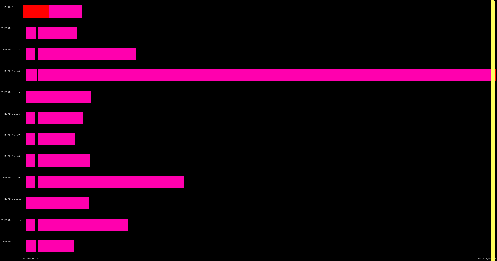
(a) Without nested tasks (Non-nested)

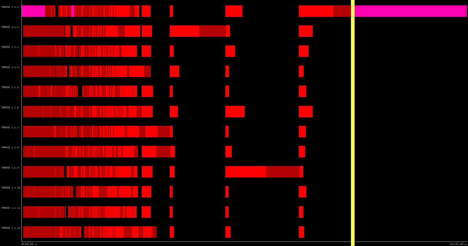
(b) With nested tasks (Nested)

Figure 2. Comparison of execution traces with or without nested tasks for bone010. The yellow line indicates the end of the parallel part.

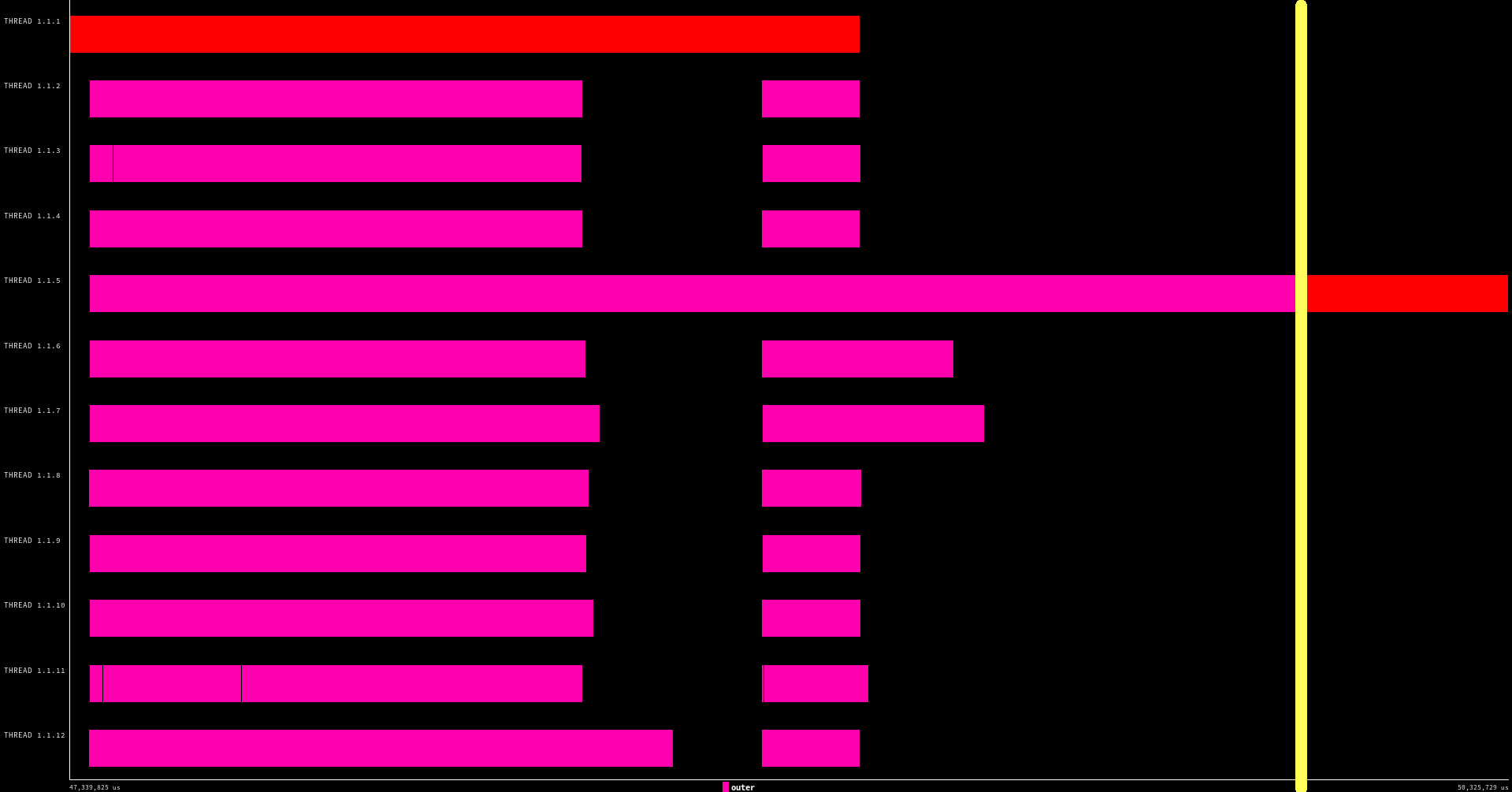
(a) Without nested tasks (Non-nested)

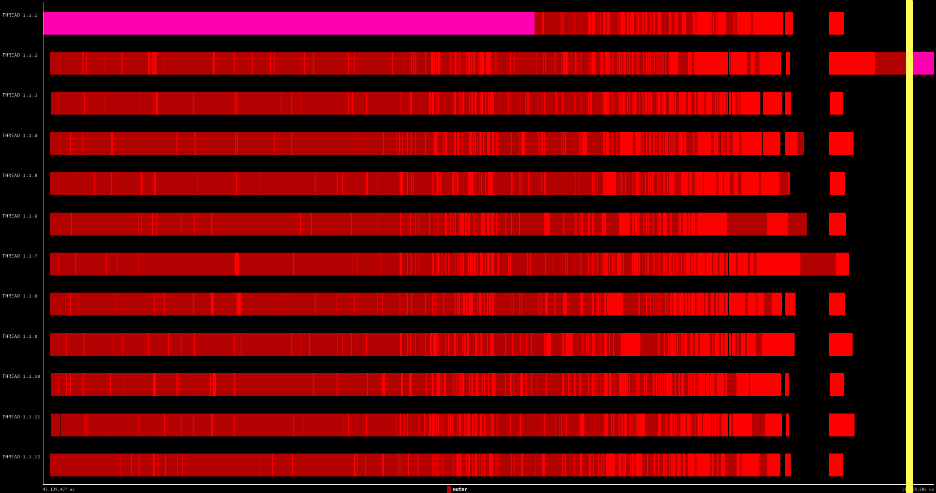
(b) With nested tasks (Nested)

Figure 3. Comparison of execution traces with or without nested tasks for inline_1. The yellow line indicates the end of the parallel part.

Figure 2 shows the execution trace of Listing 1 when inner tasks are not instantiated (top, Non-nested strategy), and when they are used (bottom, Nested strategy) for the input matrix bone010. Our complete experimental setup is described in detail in Section 5.1. The x-axis represents time while the y-axis represents different threads, 12 in this case. Each colored block corresponds to a task, and black blocks represent idle thread periods. The colors only indicate which part of the code is running. For Non-nested, as there are only outer tasks, there is only one color (pink) for them. For Nested, the two shades of red indicate whether it is an outer (dark red) or inner (light red) task. When using nested tasks, one color is used for outer tasks and another for inner tasks. As we can see, never using inner tasks usually slows down the parallel run because it does not fully expose all sources of parallelism available. However, always using nesting can also slow down the matrix factorization since task creation incurs overhead. Figure 3 shows such a case with the comparison of Non-nested (top) and Nested (bottom) strategies for the input matrix inline_1. When too many inner tasks are created, the main thread is fully dedicated to creating tasks as fast as possible and more synchronization is needed, and this becomes a bottleneck for performance. As an example with matrix boneS10, when we do not use nesting, we have 53,030 tasks and the ratio between the total time spent in task creation, scheduling and synchronization over the total time spent computing is around 11%. Mainly one thread is responsible for managing the dependencies. When using nesting, we reach 248,510 tasks and the same ratio goes up to 28% and all the threads are involved into task management. The total computing time is also increased in that case. Besides the task creation overhead problem, instantiating many tasks significantly increases the application memory footprint and sometimes overwhelms the system memory storage capacity, as Section 5 indicates.

For these reasons, we introduce selective nesting. As demonstrated by the previous examples, there is a performance trade-off between exploiting the parallelism as much as possible and the overhead of task creation. We need to determine what should be the best granularity for the tasks. Our idea is to select which outer tasks will be split in several inner tasks and which outer tasks will not. This means that, either all inner tasks inside an outer task will be used, or none of them. To select which tasks we split, we introduce a threshold value, named $D$, on the number of updates received by each supernode from the previous ones. Each update corresponds to one iteration of the inner loop, Line 7 in Listing 1: if the number of updates is higher than or equal to $D$ then the outer task is split. Otherwise, if there are not enough updates, all computation is kept embedded in the outer task. Thus, by varying $D$, we have a spectrum of heuristics to perform selective nesting with the two extreme cases being Non-nested (when $D=\infty$) and Nested (when $D=1$).

To implement selective nesting, we use the final clause of OpenMP (openmp, ) in the definition of the outer task: if the clause evaluates to True, then the task cannot have nested tasks and all task directives inside of that task are ignored. If the clause evaluates to False, then all task directives encountered inside the task are executed as usual.

4.2. The Opt-D algorithm

This section proposes the Opt-D algorithm, a heuristic to drive selective nesting. Opt-D determines the best value of $D$ depending on the input matrix, instead of using a pre-determined value. Indeed, setting a threshold of $D=100$ could be an efficient heuristic for some matrices, although it may happen that other $D$ values work better for some other sparse matrices. To explain this variety of behaviors, Figure 4 shows the distribution of outer tasks in terms of the number of inner tasks they instantiate for three different matrices: s3dkq4m2, boneS10 and G3_circuit. Each point of coordinates $(x,y)$ represents the number of outer tasks ($y$) that have $x$ updates to perform, i.e. result in the creation of $x$ inner tasks if nesting is used. Section 5.1 describes our experimental setup.

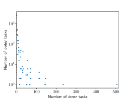
(a) s3dkq4m2

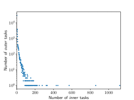
(b) boneS10

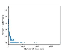
(c) G3_circuit

Figure 4. Histogram of the number of inner task per outer task. Each point of x-axis value $i$ represents the number of outer tasks that have $i$ inner tasks.

The three distributions have the same profile: there is a huge number of outer tasks that have only a few inner tasks, and there are only a few outer tasks with numerous inner tasks. The same shape of distribution can also be found for all the other sparse matrices we consider. However, there is one impact aspect that changes across different matrices: the scale. For s3dkq4m2 the maximum number of inner tasks is 505, while it is 1120 for boneS10, and 3669 for G3_circuit. This means that setting a threshold of $D=300$ for G3_circuit will create a much bigger proportion of possible inner tasks than a threshold of 300 for s3dkq4m2. It appears natural to adapt the $D$ threshold to each input matrix instead of using a predefined one.

We show the impact of $D$ on the Cholesky execution time for the three same matrices, s3dkq4m2, boneS10, and G3_circuit, in Figure 5. We also report the corresponding number of tasks (inner and outer) created. The experiment considers 12 threads on an A64FX processor. Our experimental setup is described in detail in Section 5.1.

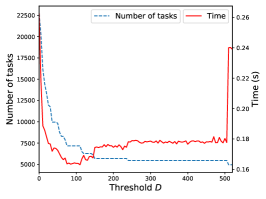
(a) s3dkq4m2

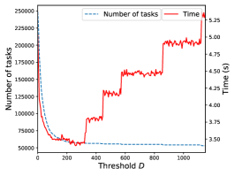
(b) boneS10

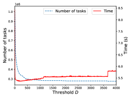
(c) G3_circuit

Figure 5. Impact of $D$ on the execution time and the number of tasks for three input matrices.

We can distinguish two different phases: First, when $D$ is small the execution time is large and decreases steadily as $D$ increases. Then, when $D$ becomes larger, the execution time starts increasing again by jumps. The first phase behavior, characterized by small values of $D$ and progressively better performance as $D$ value increases, can be explained by the overhead of task creation and destruction, which is not negligible when a large amount of tasks is created. This is the case when $D$ is small because most outer tasks instantiate many inner tasks. For the case of boneS10 for example, the number of tasks is close to 250,000 when $D$ is 1, whereas it is only around 55,000 when $D=400$. The shape of the curve for execution times actually follows that of the number of tasks in that first phase, since task instantiation is the bottleneck. Therefore, the parallel execution is slowed down by the task creation overhead.

The second phase comes from the opposite behavior: task instantiation is not anymore the bottleneck and the jumps we can see correspond to the time taken by a long outer task that does not instantiate inner tasks as $D$ increases. The more we increase $D$, the longer the execution time becomes since there are more and more long tasks executing on one thread while the other threads are idle. The limit case corresponds the Non-nested strategy. For G3_circuit, the shape is a bit different but we can still distinguish the two phases. For this matrix, the number of supernodes (hence the number of outer tasks) is huge compared to other matrices. As a comparison, even without nesting, the G3_circuit matrix creates more than 276,000 tasks. When too much nesting is introduced, i. e. $D$ is close to 1, the number of tasks skyrockets and so does the execution time, which indicates that task creation is a serious performance bottleneck.

We design the Opt-D algorithm to automatically find a good $D$ value for each input matrix. Algorithm 1 shows a high-level description of Opt-D. As input parameters it uses the size of the matrix $n$, the number of supernodes $n_{super}$ and the number of potential inner tasks of an outer task (array $C$), which CHOLMOD computes during the analysis phase.

1

input : $n$: size of the matrix

$n_{super}$: number of supernodes

$C$: array of size $n_{super}$ with the number of inner tasks of each outer task

output : $D$

2 goalTasks $\leftarrow$ max($1.1\cdot n_{super}$,$\frac{n}{14}$);

3 maxChildren $\leftarrow$ 0;

4 for $i\leftarrow 1$ to $n_{super}$ do

5       maxChildren $\leftarrow$ max(maxChildren,$C[i]$);

6      

7Create array $T$ of size maxChildren initialized at 0;

8 for $i\leftarrow 1$ to $n_{super}$ do

9       $T[C[i]]\leftarrow T[C[i]]+1$;

10      

11 $D\leftarrow$ maxChildren $+~{}1$;

12 numOuterTasks $\leftarrow$ 0;

13 numTasks $\leftarrow n_{super}$;

14 while  (numTasks $<$ goalTasks or $D>0.3\cdot$maxChildren or numOuterTasks $<\frac{n_{super}}{1000}$) and $D>0$  do

15       $D\leftarrow D-1$;

16       numOuterTasks $\leftarrow$ numOuterTasks $+~{}T[D]$;

17       numTasks $\leftarrow$ numTasks $+~{}D\cdot T[D]$;

18      

19return $D$;

Algorithm 1 Opt-D.

The first step of Opt-D is to determine a reasonable number of tasks (variable goalTasks), which is done at Line 1. We experimentally determine the values of $D$ that provide the lowest execution time for several matrices (including the ones presented in Figure 5) in order to find correlations between the different matrices. The behavior of these relevant sparse matrices indicates that allowing the ratio between the size of the matrix and the number of created tasks to be above 14 implies a too large $D$ value. Just slightly overestimating $D$ can lead to a significant increase in the execution time, as execution time sudden jumps in Figure 5 indicate. Thus, we target the smallest number of tasks which reduces this ratio just below 14. However, if the average size, in terms of number of columns, of each supernode was already below 14, the minimum number of tasks would be targeted, i.e. no nesting, according to this criteria. However, our data show that, even in this case, allowing some nesting reduces the execution time, so we require that at least 10% more tasks are created. We thus take the maximum between $\frac{n}{14}$ and $1.1\cdot n_{super}$ as the minimum number of tasks to reach, with $n$ the size of the matrix, and $n_{super}$ the number of supernodes.

The second step is to sort the outer tasks by decreasing number of inner tasks. This step is done through the application of bucket sort to the C array in the T array, through Lines 1 to 1. Once the bucket sort is done, T[i] contains the number of outer tasks that have $i$ updates, i.e. T contains the information presented in Figure 4.

The third step of the algorithm is to determine $D$ by going through the T array backwards, which corresponds to Lines 1 to 1. Additionally, we enforce $D$ to be smaller than $30\%$ of the maximum number of inner tasks in an outer task, as our preliminary analysis on the optimal $D$ value for a set of relevant sparse matrices indicates. We also ensure that at least the largest 0.1% outer tasks always instantiate other inner tasks. This takes into account the case when the largest outer tasks (in terms of number of inner tasks) account for more than 10% of new created tasks. If this occurs, only the largest tasks are split, limiting the parallelism for the supernodes that are factorized first, as big outer tasks tend to be executed at the end due to the ordering in the analyze phase.

As maxChildren is in practice much smaller than the number of supernodes, the algorithm runs in $O(n_{super})$ where $n_{super}$ is the number of supernodes. Its cost is thus negligible in front of the factorization time.

4.3. The Opt-D-Cost algorithm

This Section presents the Opt-D-Cost algorithm, which is an extension of Opt-D. Opt-D determines a threshold $D$ based on the estimated size of each outer task. If an outer task has more than $D$ (as computed by Opt-D) inner tasks, then all the inner tasks are created. However, if an inner task embeds a tiny amount of computation, it might be worth keeping it in the outer task to avoid paying the cost of task creation, which would be of the same order of magnitude.

To deal with this problem we introduce an additional threshold to drive inner task creation. An inner task is composed of one SYRK kernel and one GEMM kernel, so we estimate its cost in terms of floating-point operations using previously proposed methods based on computational complexities (trefethen97, ). If the cost of the inner task is smaller than the threshold, the task will not be created and computation will be embedded in the original outer task. Otherwise, the task is created as usual. We experimentally tuned the threshold to be 50,000 floating-point operations and we refer to this algorithm as Opt-D-Cost. OpenMP does not provide any way of controlling the task creation of a single nested task based on a condition, so the implementation was done by having the code of the inner tasks preceded by an OpenMP task directive guarded by an if-then construct.

4.4. Additional Methods to Exploit Parallelism Within Supernodes

While Sections 4.2 and 4.3 describe methods to adjust nested tasking within supernodes without exploiting any parallelism within BLAS calls, this section describes an additional method to exploit parallelism within supernodes based on multi-threaded BLAS kernels. This method sequentially factorizes supernodes via BLAS/LAPACK calls (POTRF, TRSM, SYRK and GEMM) that run on multiple threads. These multi-threaded BLAS kernels are very efficient for dense matrices, which makes them more suitable for large and dense supernodes as they require larger updates and factorizations. We refer to this method based on multi-threaded BLAS kernels as mt-BLAS. To improve our algorithms, we define a hybrid approach that switches between Opt-D-Cost (or Opt-D) and mt-BLAS. This hybrid algorithm can be summarized as follows:

• if the average supernode size is greater than 50: use mt-BLAS;

• if the average supernode size is greater than 20 and the density of the matrix, i.e. the number of non-zeros divided by the total number of cells, is below $10^{-4}$: use mt-BLAS;

• otherwise, use Opt-D-Cost (or Opt-D) with sequential BLAS calls and OpenMP task directives.

We will compare our hybrid approach to mt-BLAS in Section 5. For simplicity, we will refer to this hybrid approach as Opt-D-Cost (or Opt-D) through the end of the paper, even though depending on the input matrix, the algorithm may rely on mt-BLAS.

5. Evaluation

This section is dedicated to the performance evaluation of all the heuristics described in Section 4. Section 5.1 describes in detail our experimental setup, and Section 5.2 compares the performance of Opt-D and Opt-D-Cost with mt-BLAS on a wide range of matrices. Section 5.2 also considers two more approaches: Non-nested, which never creates inner tasks, and Nested which always does so.

5.1. Experimental setup

This subsection describes the hardware platform and the software stack we use in our experimental campaign. We consider a 4-socket A64FX (A64FX, ) machine, which implements the Armv8.2 architecture and supports SVE instructions:

• 4 sockets of 12-core A64FX CPU chips, each @2.20GHz for a total of 48 cores per node

• 32 GB of main memory HBM2

• TofuD network

We use the Red Hat Enterprise Linux Server 8.1 operating system, Fujitsu optimized BLAS kernels, and the vendor-optimized fcc 4.2.0b compiler. To support the execution of our OpenMP codes using task directives we use the OmpSs-1 19.06 as a runtime system (ompss, ). This runtime system fully supports OpenMP and makes use of nanos++ and mercurium as runtime library and compiler. Our results consider hybrid versions of the Opt-D and Opt-D-Cost algorithms that use either multi-threaded BLAS kernels or OpenMP tasks. We report the performance that these hybrid versions achieve based on the condition that selects using either multi-threaded BLAS kernels or OpenMP tasks.

Table 1. Matrices of Group 1.

Matrix Name	Number of rows	Non-zeros	Problem type
bcsstk34	588	21418	Structural
msc01050	1050	26198	Structural
bcsstk21	3600	26600	Structural
plbuckle	1282	30644	Structural
plat1919	1919	32399	2D/3D
bcsstk11	1473	23241	Structural
msc00726	726	34518	Structural
nasa1824	1824	39208	Structural
Trefethen_2000	2000	41906	Combinatorial
msc01440	1440	44998	Structural
bcsstk23	3134	45178	Structural

Table 2. Matrices of Group 2.

Matrix Name	Number of rows	Non-zeros	Problem type
nasa4704	4704	104756	Structural
crystm01	4875	105339	Materials
bcsstk15	3948	117816	Structural
bodyy4	17546	121550	Structural
aft01	8205	125567	Acoustics
bodyy5	18589	128853	Structural
bodyy6	19366	134208	Structural
bcsstk18	11948	149090	Structural
bcsstk24	3562	159910	Structural
Muu	7102	170134	Structural
nasa2910	2910	174296	Structural
t2dah_e	11445	176117	Duplicate Model Reduction
obstclae	40000	197608	Optimization
jnlbrng1	40000	199200	Optimization

Table 3. Matrices of Group 3.

Matrix Name	Number of rows	Non-zeros	Problem type
cfd2	123440	3085406	Computational Fluid Dynamics
nd3k	9000	3279690	2D/3D
shipsec8	114919	3303553	Structural
shipsec1	140874	3568176	Structural
Dubcova3	146689	3636643	2D/3D
parabolic_fem	525825	3674625	Computational Fluid Dynamics
s3dkt3m2	90449	3686223	Structural
smt	25710	3749582	Structural
ship_003	121728	3777036	Structural
ship_001	34920	3896496	Structural
cant	62451	4007383	2D/3D
offshore	259789	4242673	Electromagnetics
pdb1HYS	36417	4344765	Weighted Unidrected Graph
s3dkq4m2	90449	4427725	Structural
thread	29736	4444880	Structural
shipsec5	179860	4598604	Structural
consph	83334	6010480	2D/3D

Table 4. Matrices of Group 4.

Matrix Name	Number of rows	Non-zeros	Problem type
apache2	715176	4817870	Structural
ecology2	999999	4995991	2D/3D
tmt_sym	726713	5080961	Electromagnetics
boneS01	127224	5516602	Model Reduction
G3_circuit	1585478	7660826	Circuit Simulation
thermal2	1228045	8580313	Thermal
af_shell3	504855	17562051	Subsequent Structural
StocF-1465	1465137	21005389	Computational Fluid Dynamics
Fault_639	638802	27245944	Structural
nd24k	72000	28715634	2D/3D
inline_1	503712	36816170	Structural
Emilia_923	923136	40373538	Structural
boneS10	914898	40878708	Model Reduction
ldoor	952203	42493817	Structural
bone010	986703	47851783	Model Reduction
Hook_1498	1498023	59374451	Structural
audikw_1	943695	77651847	Structural
Flan_1565	1564794	114165372	Structural

We evaluate the different algorithms considering 60 input matrices from the SuiteSparse Matrix Collection (suitesparseMC, ). We define 4 different groups of symmetric definite positive matrices based on their number of non-zero elements:

• Group 1 is described in Table 2. It contains matrices from 10,000 to 50,000 non-zero elements.

• Group 2 is described in Table 2. It contains matrices from 100,000 to 200,000 non-zero elements.

• Group 3 is described in Table 4. It contains matrices from 3,000,000 to 6,000,000 non-zero elements.

• Group 4 is described in Table 4. It contains matrices with at least 4,800,000 non-zero elements, and they are among the largest matrices in terms of number of rows in the SuiteSparse collection.

The experiments report the average over 100 runs for matrices of Groups 1 and 2, and over 10 runs for matrices of Groups 3 and 4.

5.2. Performance evaluation of Opt-D and Opt-D-Cost

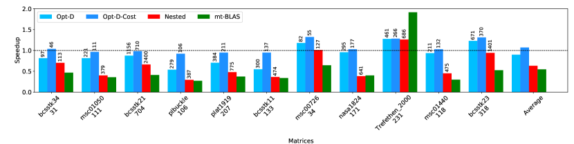
Figure 6. Speed-up relative to Non-nested of 4 algorithms on CTE-ARM using 12 threads for matrices of Group 1.

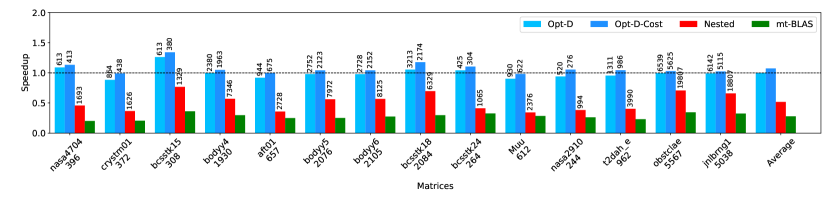
Figure 7. Speed-up relative to Non-nested of 4 algorithms on CTE-ARM using 12 threads for matrices of Group 2.

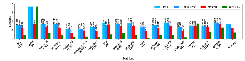
Figure 8. Speed-up relative to Non-nested of 4 algorithms on CTE-ARM using 12 threads for matrices of Group 3.

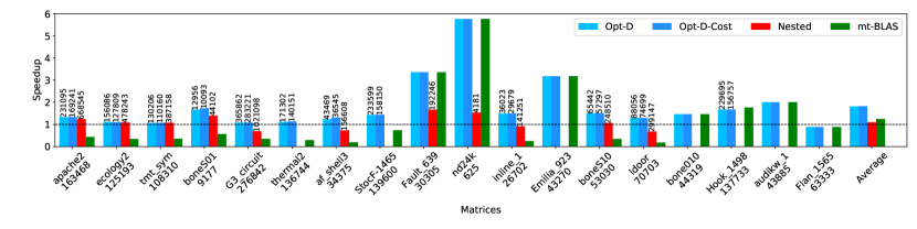
Figure 9. Speed-up relative to Non-nested of 4 algorithms on CTE-ARM using 12 threads for matrices of Group 4.

This section compares the performance of Opt-D, Opt-D-Cost, Nested, Non-nested and mt-BLAS. Figures 6, 7, 8, and 9 show the speed-up of all algorithms with respect to Non-nested for group matrices 1, 2, 3, and 4, respectively. We report the average speed-ups for each group on the right-hand side of each plot. On top of each bar, we also indicate the total number of tasks executed for each algorithm. The number of tasks executed using Non-nested, i.e. the number of supernodes for the matrix, is reported below the matrix name. Note that for mt-BLAS implementation, even when used by Opt-D and Opt-D-Cost heuristics, we do not have any number of tasks as the parallelism comes from classical multi-threading.

Figure 6 reports performance results when considering matrices belonging to Group 1. Opt-D-Cost is the only approach that provides better average performance than Non-nested since it achieves a 1.07$\times$ average speedup. Results of Figure 6 indicate that Opt-D-Cost provides very significant performance improvements with respect to Non-nested for some matrices (e.g. 1.32$\times$ for the case of msc00726). The average speed-ups of Opt-D is 0.90$\times$ for Group 1 with respect to Non-nested, which clearly indicates the benefits of adding the additional condition to drive nested parallelism that Section 4.3 introduces. We can also notice that in most cases mt-BLAS is much slower than Opt-D-Cost, averaging a speed-up of only 0.55$\times$. This is due to the size and sparsity of supernodes, which make BLAS kernels and inner tasks very short. The parallelization of the BLAS kernel then leads to poor performance, and the overhead due to creation of nested tasks is not negligible for the case of Opt-D. This can be clearly seen for matrix bcsstk11, where Opt-D-Cost has a speed-up of 0.95$\times$, compared to 0.55$\times$ for Opt-D, by removing the creation of small inner tasks. Opt-D-Cost was designed to counter this problem and thus gives a good performance overall.

Figure 7 reports the performance of all considered approaches on matrices belonging to Group 2. Nested obtains worse performance than Non-nested, a 0.52$\times$ average speed-up, while mt-BLAS only achieves a speed-up of 0.28$\times$ compared to Non-nested. The poor performance of these two techniques, Nested and mt-BLAS, is due to the sparsity and the small size of matrices supernodes. In contrast, Opt-D-Cost achieves an average speed-up of 1.07$\times$ for Group 2 with respect to Non-nested. Precisely, Opt-D-Cost is 3.84$\times$ faster than mt-BLAS. and 2.07$\times$ faster than Nested for Group 2.

For Group 3, on Figure 8, mt-BLAS has an average speed-up of 0.75$\times$, while Nested grants a 1.28$\times$ average speed-up with respect to Non-nested. Opt-D and Opt-D-Cost overcome the other approaches by reaching an average speed-up of 1.68$\times$ and 1.67$\times$ respectively. For Group 3, Opt-D-Cost is thus 1.30$\times$ faster than Nested and 2.23$\times$ faster than mt-BLAS. The performance of Opt-D and Opt-D-Cost is very similar for the 18 matrices while mt-BLAS is clearly the worst heuristic, reaching a speed-up of only 0.15$\times$ for cant. Contrarily to Group 2, Nested is a more efficient heuristic than Non-nested for Group 3, which can be explained by two facts: First, inner tasks embed a significant amount of computation. Second, when reaching the root of the elimination tree, tree parallelism experiences a significant reduction and Non-nested induces long sequential tasks at the end of the execution since supernodes are large for Group 3 matrices.

There is one special matrix in Group 3: nd3k. This matrix is much denser than the others, has less rows and columns than the others and has especially huge supernodes. While most matrices so far have an average supernode size between 5 and 25, that of nd3k is 103.45. This matrix has a few large and dense supernodes. Large and dense supernodes mean that multi-threaded BLAS kernels are efficient,which is why mt-BLAS gets a speed-up of 3.66$\times$ for nd3k, but so does our heuristics Opt-D and Opt-D-Cost as the average supernode size is well above 50.

Finally, we can derive the same conclusions for Group 4 as for Group 3. Opt-D and Opt-D-Cost are the best heuristics with average speed-ups of 1.82$\times$ and 1.83$\times$, respectively. There are several matrices where Opt-D and Opt-D-Cost use mt-BLAS: Fault_639, Emilia_923, bone010, audikw_1, Flan_1565 and nd24k. The last one is a matrix with the same properties as nd3k of Group 3, while the five others have densities smaller than $10^{-3}$ and an average supernode size between 20 and 25. Except for Flan_1565, the speed-up reached by the use of multi-threaded BLAS kernels is greater than 1$\times$ for all this subset of matrices. We can clearly see the benefits or our hybrid approach for matrices such as af_shell3, where the speed-up of mt-BLAS drops to only 0.19$\times$, while Opt-D-Cost is at 1.31$\times$. The average speed-up of mt-BLAS is 1.25$\times$, meaning that Opt-D-Cost has a 1.46$\times$ speed-up with respect to mt-BLAS. Generally, the speed-up of Opt-D and Opt-D-Cost is better than Nested, with the advantage of consuming less memory. Indeed, the speed-up for Nested is not reported for all inputs because of the memory consumption of all instantiated tasks is above the machine capacity. The total memory capacity of the A64FX machine is not enough to handle Nested, at least for one of the ten runs, for the seven following matrices: thermal2, StocF-1465, Emilia_923, bone010, audikw_1, Hook_1498, Flan_1565.

To summarize, the improvement made with Opt-D-Cost over Opt-D is more noticeable for small matrices. It thus makes Opt-D-Cost an efficient algorithm over a large number of different input matrices (a total of 60 in this evaluation). Its performance is equal or better than Non-nested, always better than Nested and is rarely beaten by mt-BLAS as we are able to detect the matrices for which it is better not to rely on a task-based decomposition. Importantly, in each group, we can see that mt-BLAS can really slow down the factorization phase for some matrices. On average over the 60 matrices, mt-BLAS, Opt-D and Opt-D-Cost achieve a speed-up of 0.75$\times$, 1.42$\times$, and 1.46$\times$, respectively, with respect to Non-nested. This means that Opt-D-Cost is on average 1.95$\times$ faster than mt-BLAS over the 60 sparse matrices we consider. The speed-up of Nested averages 0.90$\times$ over the 53 matrices for which it terminates. All source files, raw data and scripts for re-doing this evaluation are available (github, ).

6. Related work

Task-based Cholesky factorization. There is recent work on multi-threaded algorithms for sparse matrix factorization. In particular, Tang et al. (tangHybrid, ) developed a multi-threaded version of CHOLMOD for hybrid architectures, using both CPU and GPU. Their speed-up is high thanks to the use of the GPU but their parallel implementation corresponds to the use of outer tasks only. Davis et al. (davisGPU, ) also design a method for sparse Cholesky factorizations on GPUs, using subtrees and batching to take advantage of the BLAS and LAPACK kernels on a GPU. Hogg et al. (HoggCholesky, ) designed an algorithm for sparse Cholesky factorization using OpenMP. They divide supernodes in blocks to have a really fine-grained implementation but their algorithm does not change its granularity depending on the tasks and/or the input matrix as we do. Other known implementations include MUMPS (mumps, ), which is designed for distributed-memory machines with MPI, PARDISO (PARDISO, ), which is a supernodal algorithm, and WSMP (WSMP, ), which uses Pthreads. Authors of PaStiX (pastixRuntime, ) also investigated the use of a runtime-driven supernodal Cholesky factorization. Starting from the original scheduling scheme of PaStiX (pastix, ), which uses a 1D decomposition of the matrix similar to our Non-nested strategy, they study the dynamical decomposition of the updates to other supernodes into several nested tasks to accelerate the critical path of the algorithm, mainly for heterogeneous platforms. PaStiX does not take into account the sparsity of the matrix when creating nested tasks. It is thus equivalent to the Nested strategy. Note that in (pastix, ), the authors use timing models for BLAS kernels instead of considering the number of flops, but these timing models need to be calibrated just as our algorithm Opt-D and the algorithm was not task-based at the time.

Multifrontal algorithms. Multifrontal methods constitute another class of algorithms targeting matrix factorization problems. These methods divide the input matrix into several blocks, called fronts, that are operated following the order defined by the elimination tree. Contrarily to supernodal algorithms, the fronts are computed and moved along the elimination tree, instead of directly factorizing the supernodes. As such, these methods exploit the parallelism available at the elimination tree level. Multifrontal methods were introduced by Duff and Reid (duffreid, ) in the early 80s. Other works introduced node amalgamation (duffreid, ; ashcraftSparse, ), which consists in merging elimination tree nodes, creating bigger fronts and allowing more reuse of the data. It incurs additional storage and computation cost. Some early multifrontal and parallel sparse Cholesky factorizations were proposed in the early 90s (schreiberParallel, ), but they were obviously not designed to run on modern architectures, even if node amalgamation was already in place. A great survey about techniques used for general multifrontal algorithms was written in early 90s (liuMultifrontal, ). The work from Geist and Ng (GeistNgLeverage, ) describes an algorithm to leverage the cost of the subtrees in the elimination tree for Cholesky factorization. The algorithm finds a separation layer in the tree to reach an acceptable load balance (in terms of flops).

About QR and LU factorizations. Recent parallel matrix factorizations using multifrontal algorithms exist for the QR and LU methods. The method of Geist-Ng was re-used by L’Excellent and Sid-Lakhdar (mumps-shared, ) for LU factorization, while also adding the use of multi-threaded BLAS calls for the top nodes of the tree. They also switch from flops to estimated running times using models to avoid load imbalance due to the presence of many small fronts (where speed is limited) on one side and a few large fronts on another (where implementations are more efficient). However, their approach corresponds to using only non-nested tasks or multi-threaded BLAS for one node, depending on its depth in the elimination tree, and we have shown that using multi-threaded BLAS usually undermines the performance compared to a task-based approach in most cases. Davis et al. (Davis2009MultifrontralQR, ) provide an implementation for a rank-revealing QR using both parallelism in BLAS kernels and at tree level using Intel’s Threading Building Blocks software. Another fine-grained implementation of QR similar to our Nested strategy has been proposed (buttariQR, ). It uses OpenMP. This proposal assigns the creation and assembly of the fronts to independent tasks, while we assign the equivalent operations in the context of CHOLMOD to outer tasks. Previous approaches (mumpsQR, ) analyze the effect of the granularity on the performance for task-based QR factorization, based on 1D or 2D decomposition of the matrix. However, they do not provide an auto-adaptive algorithm: they run the algorithm with different parameters and report the best set for each input. For LU, Booth et al. (BoothBasker, ) developed a parallel implementation based on the Gilbert-Peierls algorithm (GilbertPeierls, ). Their approach is not based on the use of supernodes and their implementation used Kokkos (kokkos, ) as a portable framework to provide parallelism. Closer to our work in term of implementation, Ghysels et al. (HSS-Ghysels, ) use OpenMP to define a task-based implementation of multi-frontal LU factorization using different levels of nesting. They implement their own task-based linear algebra kernels so that the node parallelism does not conflict with the tree parallelism. To limit the number of tasks created, they simply take into account the depth of a node in the elimination tree so that the deeper nodes are merged with their parents. Finally, Tang (tangPHD, ) also implemented the LU factorization for hybrid architectures.

7. Conclusion

This paper presents a selective nesting approach to drive the parallel granularity of CHOLMOD, a sparse Cholesky factorization algorithm, using OpenMP. Our parallel implementation has two different types of tasks, outer and inner. The latter can be used to parallelize even more the former. To deliver the best parallel approach, we present two heuristics that determine the outer tasks for which it is better to use nested inner tasks. One of these heuristics, Opt-D, determines a good nesting threshold for any input matrix, so that the user does not have to tune the algorithm beforehand. It gives a very good performance for large matrices compared to the multi-threaded version of CHOLMOD (mt-BLAS), which relies on multi-threaded BLAS kernels. It also proves to be better than the two extreme and more classical options of having either always or never nested tasks, as the matrix sparse pattern has to be taken into account for creating the task-graph. To further increase the generality of Opt-D, we present an improved algorithm, Opt-D-Cost. By setting a threshold on the cost of the inner tasks, we decrease the execution times by avoiding the creation of small tasks. Both these heuristics run a fast algorithm before factorizing the input matrix to decide which parallel approach should be used. Results delivered by Opt-D-Cost are similar to Opt-D for large matrices and much better for small matrices. The average speed-up achieved by Opt-D-Cost compared to Non-nested is 1.07$\times$ for small matrices and 1.83$\times$ for large matrices, while mt-BLAS delivers very low performance (down to 0.15$\times$ speed-up) for some matrices. Our whole evaluation was done using OmpSs and A64FX processors.

In the future, we plan to apply our algorithms to matrix factorizations running on x86 architectures. Due to the high memory-bandwidth of A64FX processors, we expect the algorithm to be tuned to target a lower number of tasks. In addition, we plan to further improve the performance by enabling multi-threaded BLAS and LAPACK kernels at the end of the factorization only, as tree parallelism is reduced when reaching the root.

References

- (1) Ompss specification, task construct. https://pm.bsc.es/ftp/ompss/doc/spec/OmpSsSpecification.pdf.
- (2) Openmp specification, task construct. https://www.openmp.org/spec-html/5.0/openmpsu46.html.
- (3) Source code and evaluation files. https://doi.org/10.5281/zenodo.5974376.
- (4) Emmanuel Agullo, Olivier Beaumont, Lionel Eyraud-Dubois, and Suraj Kumar. Are static schedules so bad? a case study on cholesky factorization. pages 1021–1030, 2016.
- (5) Emmanuel Agullo, Alfredo Buttari, Abdou Guermouche, and Florent Lopez. Implementing multifrontal sparse solvers for multicore architectures with sequential task flow runtime systems. ACM Trans. Math. Softw., 43(2), August 2016.
- (6) Patrick R. Amestoy, Timothy A. Davis, and Iain S. Duff. Algorithm 837: Amd, an approximate minimum degree ordering algorithm. ACM Trans. Math. Softw., 30(3):381–388, September 2004.
- (7) Patrick R. Amestoy, Iain S. Duff, Jean-Yves L’Excellent, and Jacko Koster. A fully asynchronous multifrontal solver using distributed dynamic scheduling. SIAM J. Matrix Anal. Appl., 23(1):15–41, January 2001.
- (8) C. Cleveland Ashcraft, Roger G. Grimes, John G. Lewis, Barry W. Peyton, Horst D. Simon, and Petter E. Bjørstad. Progress in sparse matrix methods for large linear systems on vector supercomputers. The International Journal of Supercomputing Applications, 1(4):10–30, 1987.
- (9) J. Booth, S. Rajamanickam, and H. Thornquist. Basker: A threaded sparse lu factorization utilizing hierarchical parallelism and data layouts. 2016 IEEE International Parallel and Distributed Processing Symposium Workshops (IPDPSW), pages 673–682, 2016.
- (10) Alfredo Buttari. Fine-grained multithreading for the multifrontal qr factorization of sparse matrices. SIAM Journal on Scientific Computing, 35(4):C323–C345, 2013.
- (11) Yanqing Chen, Timothy A. Davis, William W. Hager, and Sivasankaran Rajamanickam. Algorithm 887: Cholmod, supernodal sparse cholesky factorization and update/downdate. ACM Trans. Math. Softw., 35(3), October 2008.
- (12) T. Davis. Multifrontral multithreaded rank-revealing sparse qr factorization. In Combinatorial Scientific Computing, 2009.
- (13) Timothy A. Davis and Yifan Hu. The university of florida sparse matrix collection. ACM Trans. Math. Softw., 38(1), December 2011.
- (14) J. J. Dongarra, Jeremy Du Croz, Sven Hammarling, and I. S. Duff. A set of level 3 basic linear algebra subprograms. ACM Trans. Math. Softw., 16(1):1–17, March 1990.
- (15) I. S. Duff and J. K. Reid. The multifrontal solution of indefinite sparse symmetric linear. ACM Trans. Math. Softw., 9(3):302–325, September 1983.
- (16) H. Carter Edwards, Christian R. Trott, and Daniel Sunderland. Kokkos: Enabling manycore performance portability through polymorphic memory access patterns. Journal of Parallel and Distributed Computing, 74(12):3202 – 3216, 2014. Domain-Specific Languages and High-Level Frameworks for High-Performance Computing.
- (17) G. A. Geist and E. Ng. Task scheduling for parallel sparse cholesky factorization. Int. J. Parallel Program., 18(4):291–314, jul 1990.
- (18) Pieter Ghysels, Xiaoye Li, François-Henry Rouet, Samuel Williams, and Artem Napov. An efficient multicore implementation of a novel hss-structured multifrontal solver using randomized sampling. SIAM Journal on Scientific Computing, 38, 02 2015.
- (19) J. Gilbert and Timothy Peierls. Sparse partial pivoting in time proportional to arithmetic operations. Siam Journal on Scientific and Statistical Computing, 9:862–874, 1986.
- (20) John Gilbert and Robert Schreiber. Highly parallel sparse cholesky factorization. SIAM Journal on Scientific and Statistical Computing, 13, 09 1990.
- (21) Anshul Gupta, Mahesh Joshi, and Vipin Kumar. Wsmp: A high-performance serial and parallel sparse linear solver. 01 2001.
- (22) J. D. Hogg, J. K. Reid, and J. A. Scott. Design of a multicore sparse cholesky factorization using dags. SIAM Journal on Scientific Computing, 32(6):3627–3649, 2010.
- (23) Roger A. Horn and Charles R. Johnson. Matrix Analysis. Cambridge University Press, USA, 2nd edition, 2012.
- (24) Pascal Hénon, Pierre Ramet, and Jean Roman. Pastix: A high-performance parallel direct solver for sparse symmetric definite systems. Parallel Computing, 28:301–321, 02 2002.
- (25) George Karypis and Vipin Kumar. A fast and high quality multilevel scheme for partitioning irregular graphs. SIAM Journal on Scientific Computing, 20(1):359–392, 1998.
- (26) Xavier Lacoste, Mathieu Faverge, George Bosilca, Pierre Ramet, and Samuel Thibault. Taking advantage of hybrid systems for sparse direct solvers via task-based runtimes. In 2014 IEEE International Parallel Distributed Processing Symposium Workshops, pages 29–38, 2014.
- (27) Fujitsu Limited. A64fx specifications. https://www.fujitsu.com/downloads/SUPER/a64fx/a64fx_datasheet_en.pdf.
- (28) Joseph W. H. Liu. The multifrontal method for sparse matrix solution: Theory and practice. SIAM Review, 34(1):82–109, 1992.
- (29) Joseph W.H. Liu. The role of elimination trees in sparse factorization. SIAM Journal on Matrix Analysis and Applications, 11(1):134–172, 1990.
- (30) Jean-Yves L’Excellent and Wissam M. Sid-Lakhdar. A study of shared-memory parallelism in a multifrontal solver. Parallel Computing, 40(3):34–46, 2014.
- (31) Steven C. Rennich, Darko Stosic, and Timothy A. Davis. Accelerating sparse cholesky factorization on gpus. Parallel Comput., 59(C):140–150, November 2016.
- (32) Olaf Schenk and Klaus Gärtner. Solving unsymmetric sparse systems of linear equations with pardiso. Future Generation Computer Systems, 20(3):475–487, 2004. Selected numerical algorithms.
- (33) Meng Tang. Performance Optimization For Sparse Matrix Factorization Algorithms On Hybrid Multicore Architectures. PhD thesis, University of Florida, 2020.
- (34) Meng Tang, Mohamed Gadou, and Sanjay Ranka. A multithreaded algorithm for sparse cholesky factorization on hybrid multicore architectures. Procedia Computer Science, 108:616–625, 12 2017.
- (35) Lloyd N. Trefethen and David Bau. Numerical Linear Algebra. SIAM, 1997.
- (36) Mihalis Yannakakis. Computing the minimum fill-in is np-complete. SIAM Journal on Algebraic Discrete Methods, 2(1):77–79, 1981.