Sketching Distances in Monotone Graph Classes

Abstract

We study the two-player communication problem of determining whether two vertices $x,y$ are nearby in a graph $G$, with the goal of determining the graph structures that allow the problem to be solved with a constant-cost randomized protocol. Equivalently, we consider the problem of assigning constant-size random labels (sketches) to the vertices of a graph, which allow adjacency, exact distance thresholds, or approximate distance thresholds to be computed with high probability from the labels.

Our main results are that, for monotone classes of graphs: constant-size adjacency sketches exist if and only if the class has bounded arboricity; constant-size sketches for exact distance thresholds exist if and only if the class has bounded expansion; constant-size approximate distance threshold (ADT) sketches imply that the class has bounded expansion; any class of constant expansion (i.e. any proper minor closed class) has constant-size ADT sketches; and a class may have arbitrarily small expansion without admitting constant-size ADT sketches.

1 Introduction

We are interested in understanding the power of constant-cost, public-coin, randomized communication, which has been the subject of a number of recent works [Har20, HHH23, HWZ22, CHZZ22, HHM23, HHP⁺22]. Here, two players compute a function of their inputs (with success probability at least, say, $2/3$) using a randomized protocol whose cost (number of bits communicated) is independent of the size of the inputs. Examples include the Equality problem, where two players must decide if they had the same input. In practice, such protocols are used, for example, as checksums (using, say, the SHA256 hash function).

One natural type of problem is if two players have vertices $x$ and $y$ in a graph $G$, and would like to decide if their vertices are nearby. We say $G$ belongs to a class of graphs ${\mathcal{F}}$, and we ask which classes ${\mathcal{F}}$ allow the problem to be solved by a protocol whose cost is independent of the size of $G\in{\mathcal{F}}$. An equivalent question (see e.g. [Har20, HWZ22]) is to ask for a random assignment of constant-size labels to each vertex of $G$ (where the number of bits in each label does not depend on the number of vertices of $G$), which we call sketches, in such a way that one can determine whether two vertices $x$ and $y$ are nearby from their sketches. There are a number of ways one might define “nearby”​​. To give some examples, consider the case where ${\mathcal{F}}$ is the class of hypercube graphs (whose vertices are binary strings $\{0,1\}^{n}$, with an edge between $x$ and $y$ if they differ on a single bit):

1. Adjacency in the hypercube can be computed (with probability at least $2/3$) from sketches of constant size (which follows from the Hamming distance communication protocol [HSZZ06]);

2. Distinguishing between $\mathsf{dist}(x,y)\leqslant r$ and $\mathsf{dist}(x,y)>r$ can be done with sketches of size depending only on $r$ (which also follows from the Hamming distance protocol);

3. Distinguishing between $\mathsf{dist}(x,y)\leqslant r$ and $\mathsf{dist}(x,y)>\alpha r$ (for constant $\alpha>1$) can be done with sketches of size independent of $r$ and $n$ [KOR00].

We call these adjacency sketches, small-distance sketches, and approximate distance threshold (ADT) sketches, respectively (see Section 1.2 for formal definitions). We would like to know which classes of graphs, other than the hypercubes, admit similarly efficient sketches. Sketches for deciding $\mathsf{dist}(x,y)\leqslant r$ vs. $\mathsf{dist}(x,y)>\alpha r$ in general metric spaces (especially normed spaces e.g. [Ind06, AKR18, KN19]) are well-studied, and characterizing the metrics which admit this type of sketch is a well-known open problem [SS02, AK08, Jay09, Raz17], but little is known about the natural case of path-distance metrics in graphs. Recent work [HWZ22] asked which hereditary classes of graphs admit constant-size adjacency sketches, motivated by a connection between communication complexity and graph labelling schemes. [HWZ22] also gives some examples of constant-size small-distance sketches, including for planar graphs, answering a question of [Har20].

We study the relationships between these three types of sketches for the important special case of monotone classes of graphs. A class of graphs is a set of (labelled) graphs closed under isomorphism. It is hereditary if it is closed under taking induced subgraphs, and monotone if it is closed under taking subgraphs. Monotone graph classes are ubiquitous: typical examples include minor-closed classes, graphs avoiding some subgraph $H$, or graphs with bounded chromatic number.

In this paper, we completely determine the monotone graph classes which admit constant-size adjacency sketches and constant-size (i.e. independent of the number of vertices) small-distance sketches, and show that constant-size (i.e. independent of the number of vertices and the parameter $r$) ADT sketches imply the existence of constant-size small-distance sketches. Our main tool is a new connection between communication complexity and sparsity theory of graphs [NO12]. We show that the monotone classes which admit constant-size adjacency sketches are exactly the classes with bounded arboricity, and the monotone classes which admit constant-size small-distance sketches are exactly the classes with bounded expansion. Monotone classes which admit constant-size ADT sketches must also have bounded expansion, and any class with constant expansion (i.e. any proper minor-closed class) has a constant-size ADT sketch, but on the other hand a class can have expansion growing arbitrarily slowly and yet does not admit a constant-size ADT sketch. We describe these results in more detail below.

1.1 Motivation and Related Work

Labelling schemes and sketches are important primitives for distributed computing, streaming, communication, data structures for approximate nearest neighbors, and even classical algorithms (see e.g. [KNR92, GP03, Spi03, Pel05, EIX22], and [AMS99, Ind06, AK08, Raz17, AKR18] and references therein). As such, a great deal of research has been done on finding other spaces having nice sketching and labelling properties.

One direction of research investigates the metric spaces which admit approximate distance threshold (ADT) sketches, of the third type described above, as defined in [SS02]. This is a well-known open problem in sublinear algorithms (see e.g. [AK08, Jay09, Raz17]). Here, $n$ points $X\subseteq{\mathcal{X}}$ in a metric space $({\mathcal{X}},\mathsf{dist})$, should be assigned random sketches $\mathsf{sk}:X\to\{0,1\}^{*}$ such that $\mathsf{dist}(x,y)\leqslant r$ or $\mathsf{dist}(x,y)\geqslant\alpha r$ can be determined (with probability at least $2/3$) from $\mathsf{sk}(x)$ and $\mathsf{sk}(y)$. The goal is to obtain sketches whose size depends only on $\alpha$. This problem is fairly well-understood when the metric is a norm: there is a constant-size sketch for the $\ell_{p}$ (quasi-)norm, for any $0<p\leqslant 2$ [Ind06], so any metric that can be embedded into such an $\ell_{p}$ is sketchable; conversely, sketching a norm is equivalent to embedding it into $\ell_{1-\varepsilon}$ [AKR18]. Outside of norms, the problem is less well-understood: there are sketchable metrics that are not embeddable into $\ell_{1-\varepsilon}$ [KN19].

Another direction of research investigates the classes ${\mathcal{F}}$ of graphs that admit (deterministic) labelling schemes for various functions, generally called informative labelling schemes [Pel05]. The most well-studied labelling schemes are for adjacency, introduced in [KNR92, Mul89]. The main open problem is to identify the hereditary classes of graphs that admit adjacency labelling schemes of size $O(\log n)$. A solution was suggested in [KNR92] and later conjectured in [Spi03], but recently refuted in a breakthrough of [HH22], leaving the problem wide open. Randomized adjacency labelling (i.e. adjacency sketching) was studied in [FK09, Har20, HWZ22]. It was observed in [Har20, HWZ22] that a constant-size sketch implies an $O(\log n)$ labelling scheme, as desired in the above open problem, and it was further observed in [HWZ22] that the set of hereditary graph classes which admit constant-size adjacency sketches is equivalent to the set of Boolean-valued communication problems that admit constant-cost public-coin protocols, whose structure is unknown [HHH23]. This raises the following question, which was the main motivation of [HWZ22]:

Question 1.

Which hereditary classes of graphs admit constant-size adjacency sketches?

Perhaps the next most commonly studied graph labelling problem is distance labelling [GPPR04], where the goal is to compute $\mathsf{dist}(x,y)$ from the labels (see e.g. [ADKP16, AGHP16b, FGNW17, GU21]). Intermediate between distance and adjacency labelling is the decision version of distance labelling: for given $r$, decide whether $\mathsf{dist}(x,y)\leqslant r$ from the labels. We call this small-distance labelling, following the terminology of [ABR05, GL07]. For $r=1$, this coincides with adjacency labelling. The natural generalization of constant-size adjacency sketches is to ask for small-distance sketches whose size depends only on $r$; it was shown in [Har20] that such sketches exist for trees, and in [HWZ22] that they exist for any Cartesian product graphs and any stable class of bounded twin-width (including, for example, planar graphs or any proper minor-closed class; see [GPT22]).

Question 2.

Which hereditary classes of graphs admit small-distance sketches whose size depends only on $r$?

It is common to weaken distance labelling to approximate distance labelling [GKK⁺01], where the goal is to approximate $\mathsf{dist}(x,y)$ up to a constant factor (see e.g. [Tho04, ACG12, AGHP16a]). The decision version is to distinguish, for a given $r$, between $\mathsf{dist}(x,y)\leqslant r$ and $\mathsf{dist}(x,y)>\alpha r$; we will call this problem $\alpha$-approximate distance threshold (ADT) labelling and sketching. This is a similar formulation as the distance sketching problem mentioned above, with the $n$ points from the metric space ${\mathcal{X}}$ being replaced with a size $n$ graph from a class ${\mathcal{F}}$. Despite significant interest in distance sketching and labelling, the only prior work explicitly relating the two, or studying randomized ADT labelling, appears to be the unpublished manuscript [AK08] (although there is extensive literature on the related problem of embedding graph metrics into normed spaces [Mat13, Chapter 15]; embedding planar graphs into $\ell_{1}$ with constant distortion is a major open problem [GNRS04]). This raises the following question, which is a special case of the open problem of identifying sketchable metrics:

Question 3.

Which classes of graphs admit constant-size ADT sketches?

It holds by definition (see definitions below) that a small-distance sketchable class ${\mathcal{F}}$ is adjacency sketchable, but the relationships between other types of sketching are otherwise unclear, a priori. It seems reasonable to suspect that these three types of sketching require similar conditions on the graph class ${\mathcal{F}}$; so we ask:

Question 4.

What is the relationship between adjacency, small-distance, and ADT sketching?

Finally, the adjacency and small-distance sketches we obtain in this paper turn out to be equality-based, meaning that the associated randomized communinication protocols can be simulated by deterministic communication protocols that have access to an oracle which computes Equality (we explain this more carefully below). Communication with the Equality oracle has recently become a topic of interest in communication complexity; see [GPW18, CLV19, HHH23, HWZ22, AY22, PSS23].

1.2 Our Results

In this paper, we resolve Questions 1, 2, and 4 for monotone classes of graphs, and make progress towards Question 3. The sketches we obtain usually do not assume that the classes under consideration are monotone, but our lower bounds crucially rely on this assumption. We first formally define the main three types of sketchability that we are concerned with. We will generalize these definitions in Section 2.2. For a graph class ${\mathcal{F}}$, we say:

1. ${\mathcal{F}}$ admits an adjacency sketch of size $s(n)$ if there is a function $D:\{0,1\}^{*}\times\{0,1\}^{*}\to\{0,1\}$ such that $\forall G\in{\mathcal{F}}$ with size $n$, there is a random function $\mathsf{sk}:V(G)\to\{0,1\}^{s(n)}$ satisfying

   $$\forall x,y\in V(G):\qquad\Pr\left[D(\mathsf{sk}(x),\mathsf{sk}(y))=1\iff x,y\text{ are adjacent}\right]\geqslant 2/3\,.$$

   ${\mathcal{F}}$ is adjacency sketchable if it admits an adjacency sketch of constant size.

2. ${\mathcal{F}}$ admits a small-distance sketch of size $s(n,r)$ if for every $r\in{\mathbb{N}}$ there is a function $D_{r}:\{0,1\}^{*}\times\{0,1\}^{*}\to\{0,1\}$ such that $\forall G\in{\mathcal{F}}$ with size $n$, there is a random function $\mathsf{sk}:V(G)\to\{0,1\}^{s(n,r)}$ satisfying

   $$\forall x,y\in V(G):\qquad\Pr\left[D_{r}(\mathsf{sk}(x),\mathsf{sk}(y))=1\iff\mathsf{dist}_{G}(x,y)\leqslant r\right]\geqslant 2/3\,.$$

   ${\mathcal{F}}$ is small-distance sketchable if it admits a small-distance sketch of size independent of $n$.

3. For constant $\alpha>1$, ${\mathcal{F}}$ admits an $\alpha$-ADT sketch of size $s(n)$ if for every $r\in{\mathbb{N}}$ there is a function $D_{r}:\{0,1\}^{*}\times\{0,1\}^{*}\to\{0,1\}$ such that $\forall G\in{\mathcal{F}}$ with size $n$, there is a random function $\mathsf{sk}:V(G)\to\{0,1\}^{s(n)}$ satisfying

   $$\forall x,y\in V(G):\qquad\mathsf{dist}(x,y)\leqslant r \implies\Pr\left[D_{r}(\mathsf{sk}(x),\mathsf{sk}(y))=1\right]\geqslant 2/3$$

   $$\mathsf{dist}(x,y)>\alpha r \implies\Pr\left[D_{r}(\mathsf{sk}(x),\mathsf{sk}(y))=0\right]\geqslant 2/3\,.$$

   For a constant $\alpha>1$, we say that ${\mathcal{F}}$ is $\alpha$-ADT sketchable if ${\mathcal{F}}$ admits an $\alpha$-ADT sketch with size independent of $n$. ${\mathcal{F}}$ is ADT sketchable if there is a constant $\alpha>1$ such that ${\mathcal{F}}$ is $\alpha$-ADT sketchable. We discuss some nuances of ADT sketch size in Section 5.

Our results imply the following hierarchy, which answers Question 4 for monotone classes of graphs. Let $\mathsf{ADJ}$ be the adjacency sketchable monotone graph classes, $\mathsf{SD}$ the small-distance sketchable monotone graph classes, and $\mathsf{ADT}$ the ADT sketchable monotone graph classes. Then

$$\mathsf{ADT}\subsetneq\mathsf{SD}\subsetneq\mathsf{ADJ}\,.$$

That $\mathsf{SD}\subseteq\mathsf{ADJ}$ follows by definition, and $\mathsf{SD}\neq\mathsf{ADJ}$ is witnessed by the arboricity-2 graphs (as observed in [Har20]). Our contribution to this hierarchy is $\mathsf{ADT}\subsetneq\mathsf{SD}$ (which does not necessarily hold for non-monotone classes, see Example 5.2), a complete characterization of the sets $\mathsf{SD}$ and $\mathsf{ADJ}$, and some results towards a characterization of $\mathsf{ADT}$.

1.2.1 Adjacency Sketching

We resolve Question 1 for monotone classes by showing that they are adjacency sketchable if and only if they have bounded arboricity. Moreover, we obtain an adjacency sketch of size at most linear in the arboricity, and show that this is best possible. The arboricity of a graph $G$ is the minimum integer $k$ such that the edges of $G$ can be partitioned into $k$ forests. A class ${\mathcal{F}}$ has arboricity at most $k$ if all graphs $G\in{\mathcal{F}}$ have arboricity at most $k$. If there exists some constant $k$ such that ${\mathcal{F}}$ has arboricity at most $k$, we say ${\mathcal{F}}$ has bounded arboricity.

Theorem 1.1.

Any class of arboricity at most $k$ has an adjacency sketch of size $O(k)$, and any monotone class containing a graph of arboricity $k$ requires adjacency sketches of size $\Omega(k)$. In particular, any monotone class ${\mathcal{F}}$ is adjacency sketchable if and only if ${\mathcal{F}}$ has bounded arboricity.

All proofs for adjacency sketching are in Section 3. Using standard random hashing and the adjacency labelling scheme of [KNR92], it is easy to see that any class of bounded arboricity is adjacency sketchable; this was stated explicitly in [Har20, HWZ22] (the latter giving slightly improved sketch size) and the result for trees also appeared in [FK09]. We prove the converse for monotone classes (which does not hold for hereditary classes in general [HWZ22]). We use a counting argument to show that for any graph $G$ of arboricity $d$, the class of all spanning subgraphs of $G$ requires adjacency sketches of size $\Omega(d)$; our approach is inspired by the recent proof of [HHH22, HHH23] that refuted a conjecture of [HWZ22] regarding adjacency sketchable graph classes (see Conjecture 3.5), and we find that the subgraphs of the hypercube are a more natural counterexample to the conjecture of [HWZ22].

The hashing-based sketch uses randomization only to compute Equality subproblems; i.e. it can be simulated by a constant-cost deterministic communication protocol with access to a unit-cost Equality oracle. This type of sketch is called equality-based in [HWZ22]. Equality-based sketches imply some structural properties of the graph class, such as the strong Erdős-Hajnal property [HHH23]. Recent work has studied the power of the Equality oracle and found that it does not capture the full power of randomization [CLV19, HHH23, HWZ22]; in particular, the Boolean hypercubes (and any Cartesian product graphs) are adjacency sketchable, but not with an equality-based sketch [HHH23, HWZ22]. Our result shows that Equality captures the power of randomization for sketching monotone classes of graphs. In fact, it is only necessary to compute a disjunction of equality checks, which we think of as the simplest possible type of sketch. In terms of graph structure, a constant-size equality-based sketch means that the graph can be written as the Boolean combination of a constant number of equivalence graphs; if the Boolean combination is a disjunction, then the graph may simply be covered by a constant number of equivalence graphs.

We remark that sketches (especially small-distance or ADT sketches) which compute a disjunction of equality checks can be used to obtain locality-sensitive hashes, a widely-used algorithmic tool introduced in [IM98]. Almost all of our positive results are of this type. See Remark 2.4.

1.2.2 Small-Distance Sketching

We answer Question 2 by proving that the monotone graph classes that are small-distance sketchable are exactly those with bounded expansion (as in [NO12]); see Definition 2. Informally, bounded expansion means that the edge density of a graph increases only as a function of $r$ when contracting subgraphs of radius $r$ into a single vertex. Many graph classes of theoretical and practical importance have bounded expansion, including bounded-degree graphs, proper minor-closed graph classes, and graphs of bounded genus [NO12], along with many random graph models and real-world graphs [DRR⁺14].

To state our theorem, we briefly describe another type of sketch that generalizes small-distance sketching, called first-order sketching. A graph class ${\mathcal{F}}$ is first-order sketchable if any first-order (FO) formula $\phi(x,y)$ over the vertices and edge relation of the graph (with two free variables whose domain is the set of vertices) is sketchable (see Section 2.2). This type of sketch was introduced in [HWZ22] and generalizes small-distance sketching, along with (for example) testing whether vertices $x,y$ belong to a subgraph isomorphic to some fixed graph $H$. We show that, for monotone graph classes, first-order sketchability is equivalent to small-distance sketchability. All proofs for small-distance sketching are in Section 4.

Theorem 1.2.

Let ${\mathcal{F}}$ be a monotone class of graphs. Then the following are equivalent:

1. ${\mathcal{F}}$ is small-distance sketchable;

2. ${\mathcal{F}}$ is first-order sketchable;

3. ${\mathcal{F}}$ has bounded expansion.

The implications $(3)\implies(2)\implies(1)$ do not require monotonicity. $(2)\implies(1)$ holds by definition. The proof of $(3)\implies(2)$ is straightforward, but relies on a structural result of [GKN⁺20] whose proof is highly technical. We actually get the stronger result that any class with structurally bounded expansion (i.e. any class that is a first-order transduction of a class with bounded expansion) is first-order sketchable, which improves the results of [HWZ22]. It was proved in [HWZ22], using structural results of [GPT22], that any stable class of bounded twin-width is first-order sketchable. A stable class has bounded twin-width if and only if it is a transduction of a class of bounded sparse twin-width [GPT22]. Every class of bounded sparse twin-width has bounded expansion, but the converse does not hold (e.g. for cubic graphs) [BGK⁺21], so our result generalizes the result of [HWZ22]. It essentially follows from using the structural results of [GKN⁺20] instead of [GPT22]. Another interesting consequence of our result, in conjunction with concurrent work of [HHP⁺22], is that graph classes with structurally bounded expansion can be represented as a type of constant-dimensional geometric intersection graphs; see Corollary 4.8.

Our proof of $(1)\implies(3)$ (Section 4.5) requires our proof of Theorem 1.1 and some results in sparsity theory [KO04, NO12]. We actually prove a stronger statement: for any monotone class ${\mathcal{F}}$, the existence of a sketch for deciding $\mathsf{dist}(x,y)\leqslant r$ vs. $\mathsf{dist}(x,y)>5r-1$, with size depending only on $r$, implies bounded expansion. Under a conjecture of Thomassen [Tho83], we can replace the constant 5 with any arbitrarily large constant; see the remark after Conjecture 4.16. Note that, even with a constant-factor gap between distance thresholds, this problem is distinct from ADT sketching, since the small-distance sketch size is allowed to depend on $r$. If we could replace the constant 5 with any arbitrarily large constant, this would immediately imply $\mathsf{ADT}\subseteq\mathsf{SD}$.

We also present a more direct proof of $(3)\implies(1)$, without going through first-order sketching, that allows for quantitative results. Going through first-order sketching (as was also done in [HWZ22]) proves the existence of a function $f(r)$ bounding the sketch size, without giving it explicitly. We obtain explicit bounds in terms of the weak coloring number [NO12], written as $\mathrm{wcol}_{r}({\mathcal{F}})$ for any $r\in{\mathbb{N}}$ (Definition 3). Using known bounds on the weak coloring number [vdHOQ⁺17], we obtain the following corollary. As was the case for adjacency sketching, we observe that this proof (unlike the more general one for first-order sketching) produces sketches that only use randomization to compute a disjunction of Equality checks, establishing that this extremely simple type of sketch suffices for monotone classes.

Corollary 1.3.

Any graph class ${\mathcal{F}}$ with bounded $\mathrm{wcol}_{r}({\mathcal{F}})$ admits a small-distance sketch of size $O(r+\mathrm{wcol}_{r}({\mathcal{F}})\log(\mathrm{wcol}_{r}({\mathcal{F}})))$. In particular, planar graphs admit a small-distance sketch of size $O(r^{3}\log r)$, and the class of $K_{t}$-minor-free graphs admits a small-distance sketch of size $O(r^{t-1}\log r)$. Furthermore, planar graphs admit a small-distance labelling scheme of size $O(r^{3}\log n)$ and $K_{t}$-minor-free graphs admit a small-distance labelling scheme of size $O(r^{t-1}\log n)$.

Although it is not necessary for our main goal, it may be desirable for large values of $r$ to have small-distance sketches with smaller dependence on $r$, at the expense of some dependence on the graph size $n$. We present a proof that, for any fixed surface $\Sigma$, the class of graphs which can be embedded in $\Sigma$ admits a small-distance labelling scheme of size $O(r\log^{2}n)$; see Theorem 4.19. This proof, using the layering technique of [RS84, Epp00], is due to Gwenaël Joret (personal communication); we thank him for allowing us to include it here.

1.2.3 Approximate Distance Sketching

In light of Theorem 1.2, a reasonable question is whether ADT sketching for monotone classes is also determined by expansion. Our first result is that bounded expansion is necessary. All proofs on approximate distance sketching are in Section 5.

Theorem 1.4.

If a monotone class ${\mathcal{F}}$ is ADT sketchable, then it has bounded expansion.

Combined with Theorem 1.2, this proves $\mathsf{ADT}\subseteq\mathsf{SD}$. Our proof uses a recent and fairly involved result in extremal graph theory [LM20], along with the theory of sparsity [NO12], to show that an $\alpha$-ADT sketch for a monotone class ${\mathcal{F}}$ of unbounded expansion could be used to get a constant-size sketch for deciding $\mathsf{dist}(x,y)\leqslant 1$ vs. $\mathsf{dist}(x,y)>\alpha$ in arbitrary graphs, which (as we show) is a contradiction.

We are then concerned with the converse. We show that the class of max-degree 3 graphs, which has expansion exponential in $r$ [NO08], is not ADT sketchable. After proving this theorem, we learned of an unpublished result [AK08] which proves a $\Theta(\log(n)/\alpha)$ bound for one-way communication of the $\alpha$-ADT problem on degree-3 expander graphs. This could be used in place of our theorem to get the same qualitative (constant vs. non-constant) results, but not the quantitative bound: note that communication complexity cannot give sketching or labelling lower bounds better than $\Theta(\log n)$.

Theorem 1.5.

For any $\alpha>1$, any $\alpha$-ADT sketch for the class of graphs with maximum degree 3 has size at least $\Omega(n^{\tfrac{1}{4\alpha}-\varepsilon})$, for any constant $\varepsilon>0$.

This establishes that $\mathsf{ADT}\neq\mathsf{SD}$ (and negatively answers open problem 2 of [AG06] about approximate distance labels for bounded-degree graphs, which [AK08] does not). But max-degree 3 graphs have exponential expansion. Smaller bounds on the expansion are associated with structural properties: for example, in monotone classes, polynomial expansion is equivalent to the existence of strongly sublinear separators [DN16]. One may then wonder if smaller bounds on the expansion suffice to guarantee ADT sketchability. We prove that this is not the case for two natural examples: subgraphs of the 3-dimensional grid (with polynomial expansion [NO12]), and subgraphs of the 2-dimensional grid with crosses (with linear expansion [Dvo21]) are not ADT sketchable. For this we require our Theorem 1.5.

Proposition 1.6.

For the class of subgraphs of the 3-dimensional grid (the Cartesian product of 3 paths), and the class of subgraphs of the 2-dimensional grid with crosses (the strong product of 2 paths), an $\alpha$-ADT sketch requires size at least $n^{\Omega(1/\alpha)}$.

We strengthen this result by showing that one can obtain monotone classes of graphs with expansion that grows arbitrarily slowly, which are not ADT sketchable.

Theorem 1.7.

For any function $\rho$ tending to infinity, there exists a monotone class of expansion $r\mapsto\rho(r)$ that is not ADT sketchable. Moreover, for any $\varepsilon>0$, there exists a monotone class ${\mathcal{F}}$ of expansion $r\mapsto O(r^{\varepsilon})$, such that, if ${\mathcal{F}}$ admits an $\alpha$-ADT sketch of size $s(n)$, then we must have $s(n)=n^{\Omega(1/\alpha)}$.

We conclude with a brief discussion of upper bounds for ADT sketching. A number of concepts have been introduced in the literature that can be used to obtain ADT sketches, including sparse covers [AP90] and padded decompositions [KPR93]. See Section 5.5 for definitions of these concepts. We present in Theorem 5.14 a construction of ADT sketches from sparse covers.

Using the sketches obtained from sparse covers, combined with results of [Fil20] on sparse covers (based on [KPR93, FT03]), we obtain the following, which complements our Theorem 1.7; note that the graph classes with constant expansion are exactly the proper minor-closed classes [NO12].

Corollary 1.8.

For any $t\geqslant 4$, the class of $K_{t}$-minor-free graphs has a $O(2^{t})$-ADT sketch of size $O(t^{2}\log t)$. The sketch is equality-based and has one-sided error. As a consequence, every monotone class of constant expansion is ADT sketchable.

It is also relatively straightforward (see Theorem 5.16) to obtain ADT sketches from padded decompositions, with an interesting difference. These sketches may not have one-sided error and, unlike all other positive examples of sketches in this paper, they may not be equality-based. On the other hand, they are extremely small. We can use constructions of padded decompositions due to [LS10, AGG⁺19] to obtain the following remarkable corollary:

Corollary 1.9.

For any $t\geqslant 4$, the class of $K_{t}$-minor-free graphs has an $O(t)$-ADT sketch of size 2. For $g\geqslant 0$, the class of graphs embeddable on a surface of Euler genus $g$ has an $O(\log g)$-ADT sketch of size 2.

1.3 Discussion and Open Problems

The main problem left open by this paper is Question 3 for monotone classes of graphs; we have shown that a constant bound on the expansion implies ADT sketchability, while arbitrarily small non-constant bounds do not, but this does not rule out a monotone, ADT sketchable class with non-constant expansion.

We have examples showing that ADT sketching does not imply small-distance sketching, in general. But our examples are not even hereditary. Is there a hereditary class that is ADT sketchable, but not small-distance or adjacency sketchable?

Our Theorem 1.2 shows that bounded expansion implies first-order sketchability, and that for monotone classes the converse also holds. We showed more generally that classes of structurally bounded expansion are first-order sketchable. To extend our study of sketchability beyond monotone classes, it would be interesting to investigate whether the converse of this statement holds: does first-order sketchability of a hereditary class imply structurally bounded expansion?

In the preprint of this paper, we asked whether the class of subgraphs of hypercubes is a counterexample to the Implicit Graph Conjecture (IGC):

Implicit Graph Conjecture (see e.g. [KNR92, Spi03]): Does every hereditary graph class ${\mathcal{F}}$ containing at most $2^{O(n\log n)}$ graphs on $n$-vertices, admit an adjacency labeling scheme with labels of size $O(\log n)$?

This long-standing conjecture was refuted in [HH22] by a non-constructive argument, and it would be interesting to find a more natural class that refutes the conjecture. One way to design adjacency labels is to find a constant-size adjacency sketch [Har20, HWZ22], but our Corollary 3.6 shows that this doesn’t exist for the family of subgraphs of hypercubes; furthermore, prior work (e.g. [CLR20]) had not found another way of designing labels of size $O(\log n)$, suggesting that subgraphs of hypercubes might be an explicit counterexample. But, follow-up work has now found efficient labels for this class [EHZ23], leaving open the problem of finding an explicit counterexample to the IGC. A related question is whether we may characterize the monotone classes of graphs which admit adjacency labeling schemes of size $O(\log n)$.

We have focused on determining whether there exists a constant $\alpha$ such that a class is $\alpha$-ADT sketchable. It is also of interest to obtain sketches for arbitrarily small $\alpha>1$, with sketch size depending on $\alpha$. One strategy is to embed the graph isometrically into $\ell_{1}$, but this is not always the best option. We obtained a $(1+\varepsilon)$-ADT sketch for the class of forests with size $O\left(\tfrac{1}{\varepsilon}\log\tfrac{1}{\varepsilon}\right)$, but this result appeared earlier in [AK08]; this sketch is more efficient than the one obtained by embedding the trees isometrically in $\ell_{1}$. We remark that a class (monotone or not) that admits a $(1+\varepsilon)$-ADT sketch for $\varepsilon<1$ must also admit an adjacency sketch.

Finally, we point out an interesting conjecture of [HHH23], that all constant-cost public-coin communication problems contain a large monochromatic rectangle. In our terminology, using the equivalence between constant-cost communication and adjacency sketching from [HWZ22], this conjecture states that all adjacency sketchable graph classes have the strong Erdős-Hajnal property.

2 Preliminaries

2.1 Notation

Throughout the paper, $\log$ denotes the logarithm base 2, while $\ln$ denotes the natural logarithm.

We will write $\mathbf{1}[E]$ for the indicator variable for the event $E$, which takes value 1 if $E$ is true.

Given a graph $G$, the length of a path $P$ in $G$ is the number of edges of $P$. Given two vertices $x,y\in V(G)$, we define $\mathsf{dist}_{G}(x,y)$ to be the infimum of the length of a path between $x$ and $y$ in $G$; we define $\mathsf{dist}_{G}(x,y)=\infty$ if there exists no path between $x$ and $y$. Notice that $(V(G),\mathsf{dist}_{G})$ is a metric space (with possibly infinite distances between pairs of vertices if $G$ is disconnected).

The girth of a graph $G$ is defined as the size of a shortest cycle in $G$ (if $G$ is acyclic, its girth is infinite).

For a class ${\mathcal{F}}$ of graphs and an integer $n\geqslant 0$, we denote by ${\mathcal{F}}_{n}$ the family of graphs from ${\mathcal{F}}$ with $n$ vertices.

2.2 Distance and First-Order Sketching

We will require more general notions of sketching than those introduced above. For a class ${\mathcal{F}}$ of graphs, we will say that a sequence $\{f_{G}\}_{G\in{\mathcal{F}}}$ of partial functions $f_{G}:V(G)\times V(G)\to\{0,1,*\}$ is a partial function $f$ parameterized by graphs $G\in{\mathcal{F}}$. We will write $f$ to refer to this sequence.

For a graph class ${\mathcal{F}}$, we define an $f$-sketch for ${\mathcal{F}}$ as a decoder $D:\{0,1\}^{*}\times\{0,1\}^{*}\to\{0,1\}$, such that for every $G\in{\mathcal{F}}$ the following holds. There is a probability distribution over functions $\mathsf{sk}:V(G)\to\{0,1\}^{*}$, such that for all $x,y\in V(G)$,

$$f_{G}(x,y)\neq*\implies\Pr[D(\mathsf{sk}(x),\mathsf{sk}(y))=f_{G}(x,y)]\geqslant 2/3\,.$$

For a fixed $f$-sketch for ${\mathcal{F}}$ and any graph $G\in{\mathcal{F}}$, we call any probability distribution over $\mathsf{sk}:V(G)\to\{0,1\}^{*}$ that satisfies the above condition an $f_{G}$-sketch or an $f$-sketch for $G$. We define the size of the sketch as

$$\max_{G\in{\mathcal{F}}_{n}}\sup_{\mathsf{sk}}\max_{x\in V(G)}|\mathsf{sk}(x)|\,,$$

where the supremum is over the set of functions $\mathsf{sk}:V(G)\to\{0,1\}^{*}$ in the support of the distribution defined for $G$, and $|\mathsf{sk}(x)|$ is the number of bits of $\mathsf{sk}(x)$. We will say that a class ${\mathcal{F}}$ is $f$-sketchable if there exists an $f$-sketch for ${\mathcal{F}}$ with size that does not depend on the number of vertices $n$.

For a graph class ${\mathcal{F}}$, we also define an $f$-labelling scheme for ${\mathcal{F}}$ similar to above, except that for every $G\in{\mathcal{F}}$ there is a deterministic function $\ell:V(G)\to\{0,1\}^{*}$ such that for all $x,y\in V(G)$,

$$f_{G}(x,y)\neq*\;\implies\;D(\ell(x),\ell(y))=f_{G}(x,y)\,.$$

The following simple proposition (observed in [Har20, HWZ22]) relates sketches to labelling schemes:

Proposition 2.1.

If ${\mathcal{F}}$ admits an $f$-sketch of size $s(n)$, then it admits an $f$-labelling scheme of size $O(s(n)\log n)$.

We now define certain important types of $f$-sketches. Let ${\mathcal{F}}$ be a class of graphs. For any $r_{1}\leqslant r_{2}$, a distance-$(r_{1},r_{2})$ sketch for ${\mathcal{F}}$ is an $f$-sketch, as defined above, when for any graph $G$ we define the function

$$f_{G}(x,y)=\begin{cases}1&\text{ if }\mathsf{dist}_{G}(x,y)\leqslant r_{1}\\ 0&\text{ if }\mathsf{dist}_{G}(x,y)>r_{2}\\ *&\text{ otherwise.}\end{cases}$$

The size of such a sketch may depend on $r_{1}$, $r_{2}$, the number of vertices $n$, or other graph parameters.

Recall the definitions of adjacency sketchable, small-distance sketchable, and ADT sketchable. It is clear that:

1. A class ${\mathcal{F}}$ is adjacency sketchable if it is distance-$(1,1)$ sketchable;

2. A class ${\mathcal{F}}$ is small-distance sketchable if for every $r\geqslant 1$ it is distance-$(r,r)$ sketchable.

3. A class ${\mathcal{F}}$ is $\alpha$-ADT sketchable if for every $r\geqslant 1$ it is distance-$(r,\alpha r)$ sketchable, and furthermore the size of the sketch does not depend on $r$.

Following [HWZ22], we will also define FO-sketchable classes, for which we require some terminology (see e.g. [NOdMS22] for more on the following terminology). A relational vocabulary $\Sigma$ is a set of relation symbols, with each $R\in\Sigma$ having an arity $\mathrm{arity}(R)\in{\mathbb{N}}\setminus\{0\}$. A $\Sigma$-structure ${\mathcal{A}}$ consists of a domain $A$, and for each relation symbol $R\in\Sigma$ an interpretation $R^{{\mathcal{A}}}\subseteq A^{\mathrm{arity}(R)}$, which is a relation. Fix a countably infinite set $X$ of variables. Atomic formulas of vocabulary $\Sigma$ are of the form

• $x=y$ for $x,y\in X$; or,

• $R(x_{1},\dotsc,x_{r})$ for $x_{1},\dotsc,x_{r}\in X$, $R\in\Sigma$ and $r=\mathrm{arity}(R)$, which evaluates to true when $(x_{1},\dotsc,x_{r})\in R$.

First-order (FO) formulas of vocabulary $\Sigma$ are inductively defined as either atomic formulas, or a formula of the form $\neg\phi,\phi\wedge\psi,\phi\vee\psi$, or $\exists x.\phi$ or $\forall x.\psi$, where $\phi$ and $\psi$ are each FO formulas. A free variable of a formula $\phi$ is one which is not bound by a quantifier. We will write $\phi(x_{1},x_{2},\dotsc,x_{k})$ to show that the free variables of $\phi$ are $x_{1},\dotsc,x_{k}\in X$. For a value $u\in A$, we write $\phi[u/x]$ for the formula obtained by substituting the constant $u$ for the free variable $x$.

Let $\phi(x,y)$ be any formula with two free variables and relational vocabulary $\Sigma=\{E^{\prime},R_{1},\dotsc,R_{k}\}$ where $E^{\prime}$ is symmetric of arity 2 and each $R_{i}$ is unary (i.e. of arity 1). We will say that a graph class ${\mathcal{F}}$ is $\phi$-sketchable if it is $f$-sketchable for any $f$ chosen as follows. For any graph $G=(V,E)$, we choose any $\Sigma$-structure with domain $V$ where $E$ is the interpretation of the symbol $E^{\prime}$. Then set $f_{G}(u,v)=1$ if and only if $\phi(u/x,v/y)$ evaluates to true.

We remark that for any graph $G$, there are many ways to choose a $\Sigma$-structure with domain $V$ with $E$ being the interpretation of $E^{\prime}$. To be first-order sketchable, a class ${\mathcal{F}}$ must be $f$-sketchable for every such choice of functions $f_{G}$. A concrete example is that, for any $r\in{\mathbb{N}}$, we can choose the formula

$$\phi(x,y)=\exists u_{1},u_{2},\dotsc,u_{r-1}:(E^{\prime}(x,u_{1})\vee x=u_{1})\wedge(E^{\prime}(u_{1},u_{2})\vee u_{1}=u_{2})\wedge\dotsm\wedge(E^{\prime}(u_{r},y)\vee u_{r}=y)\,,$$

which evaluates to true if and only if $\mathsf{dist}_{G}(x,y)\leqslant r$.

2.3 Equality-Based Labelling Schemes and Sketches

An equality-based labelling scheme is one which assigns to each vertex a deterministic label, comprising a data structure of size $s$ that holds $k$ “equality codes”​​, which can be used only for checking equality. These labelling schemes: 1) capture the constant-cost randomized communication protocols that can be simulated by a constant-cost deterministic communication protocol with access to an Equality oracle (as studied in e.g. [CLV19, BBM⁺21, HHH23, HWZ22]); and 2) capture a common type of adjacency labels, including those of [KNR92] for bounded arboricity graphs (see [HWZ22] for others).

One might formalize these schemes in a few ways; we slightly adapt the definition from [HWZ22]. This definition is intended to simplify notation rather than optimize label size, since we care mainly about constant vs. non-constant.

Definition 1 (Equality-Based Labeling Scheme).

Let ${\mathcal{F}}$ be a class of graphs and let $f:{\mathbb{N}}\times{\mathbb{N}}\times{\mathcal{F}}\to\{0,1,*\}$ be a partial function. An $(s,k)$-equality-based $f$-labeling scheme for ${\mathcal{F}}$ is an algorithm $D$, called a decoder, which satisfies the following. For every $G\in{\mathcal{F}}$ with vertex set $[n]$ and every $x\in[n]$, there is a tuple of the form

$$\ell_{G}(x)=(p(x)\mid q(x))\,,$$

where $p(x)\in\{0,1\}^{s}$ is called the prefix and $q(x)\in{\mathbb{N}}^{k}$ is called the vector of equality codes, such that, for all $x,y\in[n]$, on inputs $\ell_{G}(x),\ell_{G}(y)$, the algorithm $D$ chooses a function $D_{p(x),p(y)}:\{0,1\}^{k\times k}\to\{0,1\}$ and outputs

$$D_{p(x),p(y)}(Q_{x,y})\,,$$

where $Q_{x,y}\in\{0,1\}^{k\times k}$ is the matrix recording whether each pair of equality codes are equal:

$$Q_{x,y}(i,j)\vcentcolon=\mathbf{1}[q(x)_{i}=q(y)_{j}]\,.$$

It is required that, for all $G\in{\mathcal{F}}$ and all $x,y\in[n]$, the output satisfies

$$D(\ell_{G}(x),\ell_{G}(y))=D_{p(x),p(y)}(Q_{x,y})=f(x,y,G)\,.$$

We make the further distinction that an $(s,k)$-equality-based labelling scheme is $(s,k)$-disjunctive if for every $G\in{\mathcal{F}}$ and $x,y\in[n]$, $D_{p(x),p(y)}(Q_{x,y})$ simply outputs a disjunction of a subset of entries of $Q_{x,y}$.

It will be convenient to introduce some alternate notation for constructing equality-based labeling schemes. We define an $(s,t,k)$-equality-based $f$-labelling scheme for ${\mathcal{F}}$ similarly to an $(s,k)$-equality-based labelling scheme, except for $G\in{\mathcal{F}}$ and $x\in[n]$, the labels are of the form

$$\ell_{G}(x)=\left[(p_{1}(x)\mid\vec{q}_{1}(x)),(p_{2}(x)\mid\vec{q}_{2}(x)),\dotsc,(p_{t}(x)\mid\vec{q}_{t}(x))\right],$$

where the vectors $p_{i}(x)\in\{0,1\}^{*}$ are called the prefixes, the entries of the vectors $\vec{q}_{i}(x)\in{\mathbb{N}}^{*}$ are called equality codes, and we must have $\sum_{i=1}^{t}|p_{i}(x)|\leqslant s$ and $\sum_{i=1}^{t}|\vec{q}_{i}(x)|\leqslant k$ (where $|v|$ denotes the number of entries of $v$). When an element $(p_{i}(x)\mid\vec{q}_{i}(x))$ in an equality-based label has $p_{i}(x)$ of size 0, we will write $(-\mid\vec{q}_{i}(x))$; similarly, we write $(p_{1}(x)\mid-)$ when $\vec{q}_{i}(x)$ is empty. Given labels of this form, it is straightforward to obtain an $(s,k)$-equality based labelling scheme by concatenating the prefixes and equality codes, along with separator symbols so that the decoder can reconstruct each $(p_{i}\mid\vec{q}_{i})$.

We emphasize that $k$ bounds the total number of equality codes associated with any vertex $x$, but not necessarily the total number of bits needed to store these codes (see Example 2.2 below, where $k=2$ but storing the codes would require $2\log n$ bits per vertex).

Example 2.2.

The adjacency labelling scheme of [KNR92] for forests can be written as an equality-based labelling scheme. For each $x$ in an $n$-vertex forest $G$ with arbitrarily rooted trees, which we assume has vertex set $[n]$, we assign the label $\ell_{G}(x)=(-\mid x,p(x))$ where $p(x)$ is the parent of $x$ if it has one, or 0 otherwise. Here the equality codes are $q(x)=(x,p(x))\in{\mathbb{N}}^{2}$. The decoder simply outputs the disjunction of $p(x)=y$ or $p(y)=x$, so in fact this is a $(0,2)$-disjunctive labeling scheme.

An equality-based labelling scheme is easily transformed into a standard deterministic labelling scheme or a sketch. The following simple proposition was observed in [HWZ22]. We sketch the proof for the sake of clarity.

Proposition 2.3.

Let ${\mathcal{F}}$ be a class of graphs and $f:{\mathbb{N}}\times{\mathbb{N}}\times{\mathcal{F}}\to\{0,1,*\}$ be a partial function. If there is an $(s,t,k)$-equality-based $f$-labelling scheme for ${\mathcal{F}}$ then there is an $f$-sketch for ${\mathcal{F}}$ of size at most $O(s+t+k\log k)$. If the scheme is disjunctive, the sketch has one-sided error: when $f(x,y,G)=1$, the sketch will produce the wrong output with probability 0.

Proof sketch.

Choose a random function $\xi:{\mathbb{N}}\to[w]$ for $w=3k^{2}$. For any vertex $x$ of a graph $G$, replace each vector $\vec{q}_{i}(x)=(q_{i,1}(x),\dotsc,q_{i,m}(x))$ with $(\xi(q_{i,1}(x)),\dotsc,\xi(q_{i,m}(x)))$. We have replaced each of the (at most) $k$ equality codes $(\vec{q}_{i}(x))_{j}$ with $\xi((q_{i}(x))_{j})$, using $k\log w=O(k\log k)$ bits in total. The sketch has size $O(s+t+k\log k)$ since we must include each $p_{i}(x)$ (using $s$ bits in total), the $O(k\log k)$ bits for the equality codes, and $O(t)$ bits to encode the symbols $(\;|\;)$.

For two vertices $x,y$, write $Q_{x,y}^{\xi}(i_{1},i_{2},j_{1},j_{2})=\mathbf{1}[\xi((\vec{q}_{i_{1}}(x))_{i_{2}})=\xi((\vec{q}_{j_{1}}(y))_{j_{2}})]$. Since there are at most $k$ equality codes in each label, there are at most $k^{2}$ equality comparisons. By the union bound, the probability that any of these comparisons have

$$\mathbf{1}[\xi((\vec{q}_{i_{1}}(x))_{i_{2}})=\xi((\vec{q}_{j_{1}}(y))_{j_{2}})]\neq\mathbf{1}[(\vec{q}_{i_{1}}(x))_{i_{2}}=(\vec{q}_{j_{1}}(y))_{j_{2}}]$$

is at most $k^{2}\cdot(1/w)=1/3$, so with probability at least $2/3$ all of the comparisons made by the decoder have the correct value, so the decoder will be correct. Note that when $(\vec{q}_{i_{1}}(x))_{i_{2}}=(\vec{q}_{j_{1}}(y))_{j_{2}}$, the random values under $\xi$ will be equal with certainty. We conclude from this that disjunctive schemes will produce sketches with one-sided error. ∎

Remark 2.4.

Disjunctive labelling schemes with $s=0$ (i.e. the $p$ values are empty) can be transformed into locality-sensitive hashes (LSH) [IM98]. A $(r_{1},r_{2},\gamma_{1},\gamma_{2})$-LSH must map any two points $x,y$ with $\mathsf{dist}(x,y)\leqslant r_{1}$ to the same hash value with probability at least $\gamma_{1}$, and map any two points $x,y$ with $\mathsf{dist}(x,y)>r_{2}$ to the same hash value with probability at most $\gamma_{2}$, where $r_{1}<r_{2}$ and $\gamma_{1}>\gamma_{2}$. By boosting the success probability of each Equality check in the disjunction, and then sampling a uniformly random term from the disjunction, one obtains an LSH with distance parameters that depend on the original sketch. All of the equality-based sketches presented in this paper, except the first-order sketches, are of this form.

3 Adjacency Sketching

In this section, we prove Theorem 1.1, and include the additional equivalent statement that ${\mathcal{F}}$ admits a constant-size disjunctive adjacency sketch. We think of disjunctive sketches as the simplest possible use of randomization in a sketch, with the theorem establishing that the simplest possible sketches are sufficient for monotone classes.

Theorem 3.1.

Let ${\mathcal{F}}$ be a monotone class of graphs. Then the following are equivalent:

1. ${\mathcal{F}}$ is adjacency sketchable.

2. ${\mathcal{F}}$ admits a constant-size disjunctive adjacency labelling scheme.

3. ${\mathcal{F}}$ has bounded arboricity.

A disjunctive labelling scheme for graphs of arboricity at most $k$ can be obtained from the adjacency labelling scheme of [KNR92], as in Example 2.2. This leads to a sketch of size $O(k\log k)$ by Proposition 2.3, which was improved slightly in [HWZ22]:

Proposition 3.2 ([HWZ22]).

Let ${\mathcal{F}}$ be any class with arboricity at most $k$. Then ${\mathcal{F}}$ admits a $(0,1,k+1)$-disjunctive adjacency labelling scheme, and an adjacency sketch of size $O(k)$.

Therefore, to prove Theorem 3.1, it suffices to prove $(1)\implies(3)$, which we will prove by contrapositive. Our proof is inspired by the recent proof of Hambardzumyan, Hatami, and Hatami [HHH23], which refuted a conjecture of [HWZ22] (see Conjecture 3.5 below). Our proof also leads to another, more natural counterexample to the conjecture of [HWZ22]: the class of subgraphs of the hypercube (Corollary 3.6).

A spanning subgraph of a graph $G=(V,E)$ is a subgraph of $G$ with vertex set $V$. Our next lemma will give a lower bound on the adjacency sketch size for the class ${\mathcal{G}}$ of spanning subgraphs of a graph $G$ of minimum degree $d$. We will actually prove the lower bound for a weaker type of adjacency sketch, which is only required to be correct on pairs $(x,y)$ that were originally edges in $G$. This stronger statement is not necessary for the current section, but will be used in the proof of Theorem 4.15.

For a graph $G=(V,E)$ and the class ${\mathcal{G}}$ of spanning subgraphs of $G$, and any subgraph $H\in{\mathcal{G}}$, we will define the partial function $\mathrm{adj}^{E}_{H}:V\times V\to\{0,1,*\}$ as

$$\mathrm{adj}^{E}_{H}(x,y)=\begin{cases}\mathrm{adj}_{H}(x,y)&\text{ if }(x,y)\in E\\ *&\text{ otherwise.}\end{cases}$$

In the remainder of this section, we view $\mathrm{adj}^{E}$ as the function $(\mathrm{adj}^{E}_{H})_{H\in{\mathcal{G}}}$ parameterized by $H\in{\mathcal{G}}$. In particular, an $\mathrm{adj}^{E}$-sketch for ${\mathcal{G}}$ computes the partial function $\mathrm{adj}^{E}_{H}$ for each $H\in{\mathcal{G}}$.

We thank an anonymous reviewer for suggesting a proof of the following lemma, which simplified and improved our original discrepancy argument.

Lemma 3.3.

Let $G=(V,E)$ be a graph of minimum degree $d$, and let ${\mathcal{G}}$ be the class of spanning subgraphs of $G$. Then any $\mathrm{adj}^{E}$-sketch for ${\mathcal{G}}$ requires size at least $\Omega(d)$.

Proof.

Fix a constant $\delta>0$ small enough that $\delta\log(e/\delta)\leqslant 1/2$. Let $n=|V|$ and $m=|E|$; we will identify $V$ with $[n]$. Assume there is an $\mathrm{adj}^{E}$-sketch for ${\mathcal{G}}$ of size $s^{\prime}$; then by standard boosting techniques, there is a sketch of size $s=O(s^{\prime})$ with error probability $\delta$ instead of $2/3$. Let $D:\{0,1\}^{s}\times\{0,1\}^{s}\to\{0,1\}$ be the decoder for the sketch.

For every subgraph $H\in{\mathcal{G}}$, we say a string $\rho\in\{0,1\}^{sn}$ is good for $H$ if the following holds. Partition $[n]=S_{1}\cup\dotsm\cup S_{n}$ such that $S_{i}\vcentcolon=\{(i-1)s+1,(i-1)s+1,\dotsc,is\}$ is the $i^{th}$ interval of $s$ consecutive indices, and write $\rho_{i}\in\{0,1\}^{s}$ for the substring of $\rho$ on indices $S_{i}$. Then $\rho$ is good for $H$ if

$$\left|\left\{(i,j):i<j,ij\in E,D(\rho_{i},\rho_{j})=H(i,j)\right\}\right|\geqslant(1-\delta)|E|\,,$$

where $H(i,j)\in\{0,1\}$ is $1$ if and only if $i,j$ are adjacent in $H$. We make two observations:

1. For every $H\in{\mathcal{G}}$ there exists $\rho\in\{0,1\}^{sn}$ that is good for $H$. Consider the random string ${\bf\rho}^{H}\vcentcolon=(\mathsf{sk}(1),\mathsf{sk}(2),\dotsc,\mathsf{sk}(n))$, where $\mathsf{sk}$ is the random $\mathrm{adj}^{E}$-sketch of size $s$ for $H$, so that ${\bf\rho}^{H}\in\{0,1\}^{sn}$ with probability 1. Then, by definition,

   $$\mathbb{E}\left[\left|\left\{(i,j):i<j,ij\in E,D({\bf\rho}^{H}_{i},{\bf\rho}^{H}_{j})=H(i,j)\right\}\right|\right]\geqslant(1-\delta)|E|\,,$$

   so ${\bf\rho}^{H}$ is good for $H$ with nonzero probability.

2. Each string $\rho\in\{0,1\}^{sn}$ is good for at most $2^{m/2}$ graphs $H\in{\mathcal{G}}$. This is because, for every string $\rho\in\{0,1\}^{sn}$, we can define $F\in{\mathcal{G}}$ as the graph obtained by putting each pair $\{i,j\}\in E$, with $i<j$, adjacent in $F$ if and only if $D(\rho_{i},\rho_{j})=1$. If $\rho$ is good for $H$, then $H(i,j)\neq F(i,j)$ for at most $\delta|E|$ pairs $\{i,j\}\in E$. Therefore the number of graphs $H$ such that $\rho$ is good for $H$ is at most

   $${m\choose\delta m}\leqslant\left(\frac{em}{\delta m}\right)^{\delta m}=2^{\delta m\log(e/\delta)}\leqslant 2^{m/2}\,,$$

   by definition of $\delta$.

From these two observations, we have $|{\mathcal{G}}|\leqslant 2^{sn}\cdot 2^{m/2}$. Since $|{\mathcal{G}}|\geqslant 2^{m}$, we conclude that $sn\geqslant m/2\geqslant dn/4$, so $s=\Omega(d)$ and therefore $s^{\prime}=\Omega(d)$. ∎

We may now complete the proof of Theorem 3.1. We aim to prove $(1)\implies(3)$, which we will prove by contrapositive: i.e. that any class of unbounded arboricity has non-constant adjacency sketch size. We will prove the following more precise version, which also completes the proof of Theorem 1.1.

Lemma 3.4.

If ${\mathcal{F}}$ contains a graph of arboricity $d$ and all its subgraphs, then ${\mathcal{F}}$ requires adjacency sketches of size $\Omega(d)$. In particular, if ${\mathcal{F}}$ is a monotone class of graphs with unbounded arboricity, then ${\mathcal{F}}$ does not admit a constant-size adjacency sketch.

Proof.

It is well-known that the degeneracy of a graph is within factor 2 of the arboricity, so ${\mathcal{F}}$ contains a graph $G$ of degeneracy $\Omega(d)$. By definition, $G$ contains a subgraph $H$ of minimum degree $\Omega(d)$. Let ${\mathcal{G}}$ be the class of spanning subgraphs of $H$. Since ${\mathcal{F}}$ contains all subgraphs of $G$, it contains all subgraphs of $H$ and thus ${\mathcal{G}}\subseteq{\mathcal{F}}$. Then by Lemma 3.3, any adjacency sketch for ${\mathcal{G}}$ must have size $\Omega(d)$, which proves the first part of the result.

If ${\mathcal{F}}$ is a monotone class of graphs with unbounded arboricity, it follows from the paragraph above that for every integer $d$ there is a lower bound of $\Omega(d)$ on the size of an adjacency sketch for ${\mathcal{F}}$; it follows that any adjacency sketch for ${\mathcal{F}}$ is of non-constant size. ∎

Theorem 1.1 now follows directly from Proposition 3.2 and Lemma 3.4.

As a consequence, we obtain a new counterexample to the following conjecture of [HWZ22]. In their terminology, a graph class ${\mathcal{F}}$ is stable if there is an absolute constant $k$ such that any sequence $a_{1},b_{1},a_{2},b_{2},\dotsc,a_{t},b_{t}$ of vertices in a graph $G\in{\mathcal{F}}$, which satisfies the condition that $a_{i},b_{j}$ are adjacent if and only if $i\leqslant j$, has length at most $t\leqslant k$.

Conjecture 3.5.

Let ${\mathcal{F}}$ be a hereditary graph class which contains at most $2^{O(n\log n)}$ graphs on $n$ vertices, and is stable, Then ${\mathcal{F}}$ admits a constant-size adjacency sketch.

We remind the reader that the conjecture was already refuted in [HHH22], using an interesting construction of a graph class that was originally used to establish a “proof barrier” in communication complexity [HHH23]. Our counterexample, the subgraphs of the hypercube, is more easily defined. The following bound on the number of subgraphs of the hypercube was observed by Viktor Zamaraev (personal communication). See [HWZ22] for a definition of stable.

Corollary 3.6.

Let ${\mathcal{F}}$ be a class of subgraphs of the hypercube. Then:

1. ${\mathcal{F}}$ is stable, and there are at most $2^{O(n\log n)}$ graphs on $n$ vertices in ${\mathcal{F}}$.

2. ${\mathcal{F}}$ is not adjacency sketchable.

Proof.

Since the $d$-dimensional hypercube of size $N=2^{d}$ has minimum degree $d=\log N$, ${\mathcal{F}}$ has non-constant adjacency sketch size. To bound the number of $n$-vertex subgraphs of the hypercubes, we first observe that there are at most $2^{O(n\log n)}$ induced subgraphs of the hypercube on $n$ vertices, which follows from the $O(\log n)$ adjacency labelling scheme for this class [Har20] (see a simpler exposition at [Har22]). It is known that any $n$-vertex induced subgraph of the hypercube has at most $O(n\log n)$ edges [Gra70], so each induced subgraph admits at most $2^{O(n\log n)}$ spanning subgraphs. Therefore the number of $n$-vertex subgraphs of the hypercube is at most $2^{O(n\log n)}\cdot 2^{O(n\log n)}=2^{O(n\log n)}$. Any monotone class of graphs which is not stable contains $K_{t,t}$, for every $t\in{\mathbb{N}}$, and therefore contains the class of all bipartite graphs. This does not hold for ${\mathcal{F}}$ (or indeed for any class containing at most $2^{O(n\log n)}$ $n$-vertex graphs), so ${\mathcal{F}}$ must be stable. ∎

4 Small-Distance Sketching

In this section we prove Theorem 1.2. This requires the notion of bounded expansion which we define in Section 4.1 before stating the formal version of the theorem in Section 4.2 and proving it in the remainder of the section.

4.1 Bounded expansion

Here we introduce the notion of expansion from sparsity theory, as discussed in [NO12, Chapter 5]. We will require some equivalence results stated in Theorem 4.1.

Definition 2 (Bounded Expansion).

Given a graph $G$ and an integer $r\geqslant 0$, a depth-$r$ minor of $G$ is a graph obtained by contracting pairwise disjoint connected subgraphs of radius at most $r$ in a subgraph of $G$. For any function $f$, we say that a class of graphs $\mathcal{G}$ has expansion at most $f$ if any depth-$r$ minor of a graph of $\mathcal{G}$ has average degree at most $f(r)$ (see [NO12, Section 5.5] for more details on this notion). We say that a class $\mathcal{G}$ has bounded expansion if there is a function $f$ such that $\mathcal{G}$ has expansion at most $f$.

Note that, for example, every proper minor-closed family has constant expansion. We now introduce two other equivalent ways to define bounded expansion: via generalized coloring numbers, and via bounded depth topological minors (both we be useful for our purposes).

Definition 3 (Weak $r$-coloring number).

Given a total order $(V,<)$ on the vertex set $V$ of a graph $G$ and an integer $r\geqslant 0$, we say that a vertex $v\in V$ is weakly $r$-reachable from a vertex $u\in V$ if there is a path of length at most $r$ connecting $v$ to $u$ in $G$, and such that for any vertex $w$ on the path, $v\leqslant w$ (in words, $v$ is the smallest vertex on the path with respect to $(V,<)$). For a graph $G$ and an integer $r\geqslant 0$, the weak $r$-coloring number $\mathrm{wcol}_{r}(G)$ is the smallest integer $k$ for which the vertex set of $G$ has a total order $(V,<)$ such that for any vertex $u\in V$, at most $k$ vertices are weakly $r$-reachable from $u$ with respect to $(V,<)$. For a graph class $\mathcal{F}$, we write $\mathrm{wcol}_{r}(\mathcal{F})$ for the supremum of $\mathrm{wcol}_{r}(G)$, for $G\in\mathcal{F}$.

Definition 4 ($(k,\ell)$-Subdivisions).

For a graph $G$ and two integers $0\leqslant k\leqslant\ell$, a $(k,\ell)$-subdivision of $G$ is any graph obtained from $G$ by subdividing each edge of $G$ at least $k$ times and at most $\ell$ times (i.e. we replace each edge of $G$ by a path with at least $k$ and an most $\ell$ internal vertices). A $(k,k)$-subdivision is also called a $k$-subdivision for simplicity;

Definition 5 (Depth-$r$ Topological Minor).

We say that $H$ is a depth-$r$ topological minor of a graph $G$ if $G$ contains a $(0,2r)$-subdivision of $H$ as a subgraph. In other words, $G$ contains a subgraph $H^{\prime}$ obtained from $H$ by subdividing each edge at most $2r$ times.

In the proof below it will be convenient to use the following equivalent definitions of bounded expansion.

Theorem 4.1 ([NO12]).

For a class $\mathcal{F}$ of graphs, the following are equivalent:

1. $\mathcal{F}$ has bounded expansion.

2. There is a function $f:\mathbb{N}\to\mathbb{N}$ such that for any $r\in\mathbb{N}$, $\mathrm{wcol}_{r}(\mathcal{F})\leqslant f(r)$.

3. There is a function $f:\mathbb{N}\to\mathbb{N}$ such that for any $r\in\mathbb{N}$ and any $G\in\mathcal{F}$, any depth-$r$ topological minor of $G$ has average degree at most $f(r)$.

The equivalence between 1. and 3. follows from Proposition 5.5 in [NO12]; while the equivalence between 1. and 2. follows from Lemma 7.11 and Theorem 7.11 in [NO12].

We will also require the following fact about the expansion of monotone classes, which is a simple consequence of Theorem 4.1 (see for instance [NO15]) combined with a result of Kühn and Osthus [KO04].

Corollary 4.2.

Let $\mathcal{F}$ be a monotone class of unbounded expansion. Then there is a constant $r\geqslant 0$, so that for any $d\geqslant 0$, $\mathcal{F}$ contains an $r$-subdivision of a bipartite graph of minimum degree at least $d$ and girth at least 6.

Proof.

Since $\mathcal{F}$ has unbounded expansion, it follows from Theorem 4.1 that there exists an $r\geqslant 0$, such that depth-$r$ topological minors of graphs in $\mathcal{F}$ have unbounded average degree. Since each edge in a depth-$r$ topological minor is subdivided at most $2r$ times, if $\mathcal{F}$ contains a depth-$r$ topological minor $H$ of average degree at least $d$, $\mathcal{F}$ also contains an $r^{\prime}$-subdivision of a subgraph $H^{\prime}$ of $H$, for some $r^{\prime}\leqslant 2r$, such that $H^{\prime}$ has average degree at least $\tfrac{d}{2r+1}$ (recall that $\mathcal{F}$ is monotone). It follows that there exists an integer $r^{\prime\prime}\leqslant 2r$ such that for infinitely many $d$, $\mathcal{F}$ contains an $r^{\prime\prime}$-subdivision of a graph of average degree at least $d$. It was proved by Kühn and Osthus [KO04] that any graph of sufficiently large average degree contains a bipartite subgraph of large minimum degree and girth at least 6. As $\mathcal{F}$ is monotone, the desired result follows. ∎

We should remark that the weaker version of Corollary 4.2 where the girth at least 6 is replaced by girth at least 4 is much simpler and does not require the result of Kühn and Osthus [KO04]: it suffices to use the simple result that any graph $G$ of large average degree contains a bipartite graph of large average degree as a subgraph (consider for instance a random bipartition of $G$).

4.2 Statement of Theorem 1.2

As in Theorem 3.1 from the previous section, we refine the theorem by showing that the sketches are in fact disjunctive.

Theorem 4.3.

Let ${\mathcal{F}}$ be a monotone class of graphs. Then the following are equivalent:

1. ${\mathcal{F}}$ is small-distance sketchable.

2. For some function $f:{\mathbb{N}}\to{\mathbb{N}}$ and every $r\in{\mathbb{N}}$, ${\mathcal{F}}$ admits a disjunctive small-distance labelling scheme of size $f(r)$.

3. ${\mathcal{F}}$ is first-order sketchable.

4. ${\mathcal{F}}$ has bounded expansion.

It holds by definition that $(3)\implies(1)$ and $(2)\implies(1)$, even without the assumption of monotonicity. We will prove $(4)\implies(3)$ and $(4)\implies(2)$ using different methods. We prove $(4)\implies(3)$ (again without the assumption of monotonicity) in Section 4.3 using the structural result of [GKN⁺20]. This proof does not give explicit bounds on the sketch size. $(4)\implies(2)$ is proved in Section 4.4 and gives explicit upper bounds on the sketch size. The final piece of the theorem, $(1)\implies(4)$, is proved in Section 4.5.

In Section 4.6, we present small-distance sketches for graphs embeddable on a given surface, with sketch size that has a smaller dependence on $r$ than in Section 4.4, but some dependence on the graph size $n$. This is desirable when $r$ is large (as a function of $n$).

4.3 Bounded Expansion Implies FO Labelling Schemes

To prove that any class of bounded expansion is first-order sketchable, we use the result of [GKN⁺20] that shows how to decompose any class of (structurally) bounded expansion into a number of graphs of bounded shrubdepth. We will require an adjacency sketch for classes of bounded shrubdepth, given below.

4.3.1 Adjacency Sketching for Bounded Shrubdepth

We must first define shrubdepth. A connection model for a graph $G$ is a rooted tree $T$ whose nodes are colored with some number $k$ of colors, such that:

• the vertices of $G$ are the leaves of $T$; and

• for two vertices $u,v\in V(G)$, whether $u$ and $v$ are adjacent in $G$ depends only on the colors of $u$ and $v$ in $T$, and the color of the lowest common ancestor of $u$ and $v$ in $T$.

To avoid ambiguity, we say $G$ has vertices while $T$ has nodes. Note that we can assume without loss of generality that all leaves are at the same distance from the root in $T$. A class $\mathcal{G}$ has bounded shrubdepth if there are some $d,k\in\mathbb{N}$ such that every $G\in\mathcal{G}$ has a connection model of depth $d$ with colors in $[k]$ (we recall that the depth of a rooted tree $T$ is the maximum number of edges on a root-to-leaf path in $T$). The reader is referred to [GHN⁺12, GHN⁺19] for more details on shrubdepth, and a number algorithmic applications in model checking.

Lemma 4.4.

Any class $\mathcal{G}$ of bounded shrubdepth admits a constant-size equality-based adjacency labelling scheme.

Proof.

Let $d,k$ be such that any graph $G\in\mathcal{G}$ has a connection model $T_{G}$ of depth $d$ using color set $[k]$. We denote by $\varphi_{G}:[k]^{3}\to\{0,1\}$ the function such that if $u$ has color $a$, $v$ has color $b$, and the lowest common ancestor of $u$ and $v$ has color $c$ in $T_{G}$, then $u$ and $v$ are adjacent in $G$ if and only if $\varphi_{G}(a,b,c)=1$. For every node $u$ of $T_{G}$, write $\chi(u)$ for the color of $u$ in the connection model.

We now construct our equality-based labels for $G$. For any vertex $x$, let $t_{0}(x),t_{1}(x),\dotsc,t_{d}(x)$ be the leaf-to-root path for $x$, where $t_{0}(x)=x$ and $t_{d}(x)$ is the root of $T_{G}$. Then the label for $x$ is the sequence $(\varphi_{G}\mid-),(\chi(t_{0}(x))\mid t_{0}(x)),\dotsc,(\chi(t_{d}(x))\mid t_{d}(x))$.

On inputs

$$(\varphi_{G}\mid-),(\chi(t_{0}(x))\mid t_{0}(x)),\dotsc,(\chi(t_{d}(x))\mid t_{d}(x))\,,$$

$$(\varphi_{G}\mid-),(\chi(t_{0}(y))\mid t_{0}(y)),\dotsc,(\chi(t_{d}(y))\mid t_{d}(y))\,,$$

the decoder operates as follows. It finds the smallest $i\in[d]$ such that $\mathbf{1}[t_{i}(x)=t_{i}(y)]$ and outputs $\varphi_{G}(\chi(t_{1}(x)),\chi(t_{1}(y)),\chi(t_{i}(x)))$.

The correctness of this labelling scheme follows from the fact that we will have $t_{i}(x)=t_{i}(y)$ if and only if the node $t_{i}(x)=t_{i}(y)$ is an ancestor of both $x$ and $y$ in $T_{G}$, so the smallest $i\in[d]$ such that $t_{i}(x)=t_{i}(y)$ identifies the lowest common ancestor of $x$ and $y$ in $T_{G}$. ∎

4.3.2 Structurally Bounded Expansion Implies First-Order Sketching

Following [GKN⁺20], we say that a class of graphs has structurally bounded expansion if it can be obtained from a class of bounded expansion by first-order (FO) transductions. We omit the precise definition of FO transductions in this paper, as they are not necessary to our discussion, and instead refer the reader to [GKN⁺20]. We just note that a particular case of FO transduction is the notion of FO interpretation, which is of specific interest to us. Consider an FO formula $\phi(x,y)$ with two free variables and relational vocabulary $\Sigma=\{F,R_{1},\dotsc,R_{k}\}$ where $F$ is symmetric of arity 2. We will say that a graph class ${\mathcal{F}}^{\prime}$ is an FO interpretation of a graph class ${\mathcal{F}}$ with respect to $\phi$ if for any graph $G^{\prime}=(V,E^{\prime})\in{\mathcal{F}}^{\prime}$ there is a graph $G=(V,E)\in{\mathcal{F}}$ and a $\Sigma$-structure with domain $V$ where $E$ is the interpretation of the symbol $F$, such that for any pair $u,v\in V$, $uv\in E^{\prime}$ if and only if $\phi(u/x,v/y)$ evaluates to true. For instance, if $\phi(u/x,v/y)$ encodes the property $\mathsf{dist}_{G}(u,v)\leqslant r$ for some fixed integer $r\geqslant 1$ (which can be written as an FO formula), then the corresponding FO interpretation of the class ${\mathcal{F}}$ is the class of all graph powers $\{G^{r}\,|\,G\in F\}$. FO transductions are slightly more involved, as it is allowed to consider a bounded number of copies of a graph before applying the formula, and then it is possible to delete vertices. We will use the following structural result for classes of structurally bounded expansion, proved in [GKN⁺20].

Theorem 4.5 ([GKN⁺20]).

A class $\mathcal{G}$ of graphs has structurally bounded expansion if and only if the following condition holds. For every $p\in\mathbb{N}$, there is a constant $m=m(p)$ such that for every graph $G\in\mathcal{G}$, one can find a family $\mathcal{F}(G)$ of vertex subsets of $G$ with $|\mathcal{F}(G)|\leqslant m$ and the following properties:

• for every $X\subseteq V(G)$ with $|X|\leqslant p$, there is $A\in\mathcal{F}(G)$ such that $X\subseteq A$; and

• the class $\{G[A]\,|\,G\in\mathcal{G},A\in\mathcal{F}(G)\}$ of induced subgraphs has bounded shrubdepth.

We directly deduce the following result.

Lemma 4.6.

Any class $\mathcal{G}$ of structurally bounded expansion admits a constant-size equality-based adjacency labelling scheme.

Proof.

Let $m$ and $\mathcal{F}$ be given by applying Theorem 4.5 to $\mathcal{G}$ with $p=2$. By definition, for every graph $G\in\mathcal{G}$ and every pair of vertices $u,v\in V(G)$, there is a set $A\in\mathcal{F}(G)$ containing $u$ and $v$. Moreover, $\mathcal{F}(G)$ contains at most $m$ sets and the family $\mathcal{C}$ of all graphs $G[A]$, for $G\in\mathcal{G}$, and $A\in\mathcal{F}(G)$, has bounded shrubdepth. It follows from Lemma 4.4 that there is a constant-size equality-based adjacency labelling scheme for $\mathcal{C}$. We denote the decoder of this scheme by $D$, and the corresponding labels as $\ell_{G[A]}$.

Consider some graph $G\in\mathcal{G}$, and let $\mathcal{F}(G)=\{A_{1},\ldots,A_{m}\}$ (for convenience we consider $\mathcal{F}(G)$ as a multiset of size exactly $m$, that is, some sets $A_{i}$ might be repeated). For each vertex $x$ of $G$ and $i\in[m]$, we write $a(x)=(a_{1}(x),\dotsc,a_{m}(x))$ where $a_{i}(x)=\mathbf{1}[x\in A_{i}]$. Then we define the label for $x$ by taking the prefix $a(x)$ and appending the labels $\ell_{G[A_{i}]}(x)$ for each induced subgraph $G[A_{i}]\in\mathcal{C}$ to which $x$ belongs. Given the labels for vertices $x$ and $y$, the decoder finds any $i\in[m]$ such that $a_{i}(x)=a_{i}(y)=1$; and outputs $D(\ell_{G[A_{i}]}(x),\ell_{G[A_{i}]}(y))$. Such a number $i\in[m]$ always exists due to Theorem 4.5. The correctness of this labelling scheme follows from Theorem 4.5 and Lemma 4.4. ∎

Since FO-transductions compose (see e.g. [NOdMS22]), sketching FO formulas in a class of structurally bounded expansion is equivalent to sketching adjacency in another class of structurally bounded expansion. We obtain the following direct corollary of Theorem 4.6.

Corollary 4.7.

Any class $\mathcal{G}$ of structurally bounded expansion is first-order sketchable.

As the property $\mathsf{dist}_{G}(x,y)\leqslant r$ can be written as an FO formula, this directly implies that classes of bounded expansion are small-distance sketchable. However, this does not tell anything on the size of the sketches as a function of $r$, unlike the approach using weak coloring numbers described in the next section.

We also observe another interesting corollary, that graph classes of structurally bounded expansion can be represented as constant-dimensional geometric intersection graphs. This follows from our lemma in conjunction with concurrent work of [HHP⁺22]. We require the notion of sign-rank. The sign-rank $\mathrm{rank}_{\pm}(M)$ of a sign matrix $M\in\{\pm 1\}^{n\times n}$ is the minimum rank $r$ of a matrix $R\in\mathbb{R}^{n\times n}$ such that $M(i,j)=\mathrm{sign}(R_{i,j})$ for all $i,j\in[n]$. Equivalently, $\mathrm{rank}_{\pm}(M)$ is the minimum dimension $d$ such that $M$ can be represented as a $d$-dimensional point-halfspace arrangement with halfspaces through the origin; i.e. $M_{i,j}=\mathrm{sign}(\left\langle u_{i},v_{j}\right\rangle)$ where $u_{i},v_{j}$ are unit vectors assigned to each row $i$ and column $j$.

For any graph $G$ on $n$ vertices, we can define its adjacency sign-matrix as the matrix $M\in\{\pm 1\}^{n\times n}$ with $M_{i,j}=1$ if and only if $i,j$ are adjacent in $G$. We say that a class ${\mathcal{G}}$ of graphs has bounded sign-rank if there exists a constant $r$ such that for every $G\in{\mathcal{G}}$, the sign-rank of the adjacency sign-matrix of $G$ is at most $r$. A graph class ${\mathcal{G}}$ with bounded sign-rank is therefore a type of constant-dimensional geometric intersection graph; if ${\mathcal{G}}$ has bounded sign-rank, then ${\mathcal{G}}$ is semi-algebraic, (and it is not known whether having bounded sign-rank is equivalent to being semi-algebraic [HHP⁺22]).

Corollary 4.8.

Any class $\mathcal{G}$ of structurally bounded expansion has bounded sign-rank.

Proof.

A result of [HHP⁺22] is that for every $M\in\{\pm 1\}^{n\times n}$, $\mathrm{rank}_{\pm}(M)\leqslant 4^{\mathsf{D}^{\textsc{Eq}}(M)}$, where $\mathsf{D}^{\textsc{Eq}(M)}$ is the deterministic communication cost of $M$ with access to an Equality oracle. ${\mathcal{G}}$ having a constant-size equality-based adjacency labelling scheme is equivalent to the existence of a constant $c$ such that $\mathsf{D}^{\textsc{Eq}}(M)\leqslant c$ for every adjacency sign-matrix $M$ of a graph in ${\mathcal{G}}$. Therefore every adjacency sign-matrix $M$ for graphs $G\in{\mathcal{G}}$ has $\mathrm{rank}_{\pm}(M)\leqslant 4^{c}$. ∎

Remark 4.9.

A very recent result of Dvořák [Dvo23, Corollary 9], which appeared after our paper was made public, can also be used to give an alternative proof of the result that any class of structurally bounded expansion is small-distance sketchable. The drawback is that his result applies to small-distance sketching (rather than first-order sketching), but the benefit is that the small-distance sketch for a vertex $v$ in a given graph $G$ can be obtained by taking a constant number of adjacency sketches of the vertices in a small ball around $v$ in $G$. This approach is more general than the approach we take in the next section, which considers classes of bounded expansion instead of classes of structurally bounded expansion.

4.4 Bounded Expansion Implies Small-Distance Sketching

Recall the definition of weak $r$-coloring number from Definition 3. We give a quantitative bound on the small-distance sketch of any graph class $\mathcal{F}$ in terms of $\mathrm{wcol}_{r}(\mathcal{F})$. Recall from Theorem 4.1 that any class with bounded expansion has $\mathrm{wcol}_{r}(\mathcal{F})\leqslant f(r)$ for some function $f(r)$; therefore we obtain the existence of small-distance sketches for any class of bounded expansion.

Theorem 4.10.

For any $r\in{\mathbb{N}}$, any class ${\mathcal{F}}$ has an $(0,r,\mathrm{wcol}_{r}({\mathcal{F}}))$-disjunctive distance-$(r,r)$ labelling scheme.

Proof.

Let $G\in{\mathcal{F}}$, and consider a total order $(V,\prec)$ such that for any vertex $x\in V$, at most $\mathrm{wcol}_{r}({\mathcal{F}})$ vertices are weakly $r$-reachable from $v$ in $G$ with respect to $(V,\prec)$. We say that vertex $y\in V$ has $x$-rank $k$ if $y$ is weakly $k$-reachable from $x$ but not weakly $(k-1)$-reachable from $x$. For each vertex $x$ and $k\in[r]$, write $S_{k}(x)$ for the set of vertices $y$ with $x$-rank $k$.

We construct a disjunctive labelling scheme as follows. Each vertex $x$ is assigned the label

$$(-\mid\vec{q}_{1}(x)),(-\mid\vec{q}_{2}(x)),\dotsc,(-\mid\vec{q}_{r^{\prime}}(x))$$

where $r^{\prime}\leqslant r$ is the maximum number such that $S_{r^{\prime}}(x)\neq\emptyset$, and the equality codes $\vec{q}_{i}(x)$ are names of vertices in the set $S_{i}(x)$. Each label contains at most $\mathrm{wcol}_{r}(G)$ equality codes. Given labels for $x$ and $y$, the decoder outputs 1 if and only if there exist $0\leqslant i,j\leqslant r$ such that $i+j\leqslant r$ and $S_{i}(x)\cap S_{j}(y)\neq\emptyset$, which can be checked using the equality codes in $\vec{q}_{i}(x)$ and $\vec{q}_{j}(y)$.

Suppose that $\mathsf{dist}_{G}(x,y)\leqslant r$ and let $P\subseteq V(G)$ be a path of length $\mathsf{dist}_{G}(x,y)$. Let $z\in P$ be the minimal element of $P$ with respect to $\prec$. Then $z$ is weakly $i$-reachable from $x$ and weakly $j$-reachable from $y$, for some values $i,j$ such that $i+j\leqslant r$. Then $z\in S_{i}(x)\cap S_{j}(y)$, so the decoder will output 1 given the labels for $x$ and $y$. On the other hand, if the decoder outputs 1, then there are values $i,j$ such that $i+j\leqslant r$ and $S_{i}(x)\cap S_{j}(y)\neq\emptyset$. Let $z\in S_{i}(x)\cap S_{j}(y)$, so that $z$ is weakly $i$-reachable from $x$ and weakly $j$-reachable from $y$. Then $\mathsf{dist}_{G}(x,y)\leqslant\mathsf{dist}_{G}(x,z)+\mathsf{dist}_{G}(z,y)\leqslant i+j\leqslant r$. ∎

We noticed after proving this result that a similar idea was used in [GKS17, Lemma 6.10] to obtain sparse neighborhood covers in nowhere-dense classes.

We will need the following quantitative results for planar graphs and graphs avoiding some specific minor, due to [vdHOQ⁺17].

Theorem 4.11 ([vdHOQ⁺17]).

For any planar graph $G$, and any integer $r\geqslant 0$, $\mathrm{wcol}_{r}(G)\leqslant(2r+1){r+2\choose 2}=O(r^{3})$.

Theorem 4.12 ([vdHOQ⁺17]).

For any integer $t\geqslant 3$, any graph $G$ with no $K_{t}$-minor, and any integer $r\geqslant 0$, $\mathrm{wcol}_{r}(G)\leqslant{r+t-2\choose t-2}(t-3)(2r+2)=O(r^{t-1})$.

In the proof of Theorem 4.10, the equality codes are just the names of vertices; so we can use $\lceil\log n\rceil$ bits to encode each of the $\mathrm{wcol}_{r}({\mathcal{F}})$ equality codes to obtain an adjacency label. Then, combined with Proposition 2.3, we obtain the following corollary:

Corollary 4.13.

If a class $\mathcal{F}$ has bounded expansion, then ${\mathcal{F}}$ has a small-distance sketch of size at most $O(r+\mathrm{wcol}_{r}({\mathcal{F}})\log(\mathrm{wcol}_{r}({\mathcal{F}})))$. If ${\mathcal{F}}$ is the class of planar graphs, then the sketch has size $O(r^{3}\log r)$ and if ${\mathcal{F}}$ is the class of $K_{t}$-minor free graphs for some fixed integer $t\geqslant 3$, then the sketch has size $O(r^{t-1}\log r)$. Furthermore, ${\mathcal{F}}$ admits a distance-$(r,r)$ labelling scheme of size $O(r+\mathrm{wcol}_{r}({\mathcal{F}})\log n)$; if ${\mathcal{F}}$ is the class of planar graphs, then the scheme has size $O(r^{3}\log n)$ and if ${\mathcal{F}}$ is the class of $K_{t}$-minor free graphs, then the scheme has size $O(r^{t-1}\log n)$.

Remark 4.14.

The fact that the sketch size is independent of the number of vertices in Corollary 4.13 implies that the scheme actually works for infinite graphs. It was proved in [HMŠ⁺21] that for infinite graphs $G$, $\mathrm{wcol}_{r}(G)$ is the supremum of $\mathrm{wcol}_{r}(H)$ for all finite subgraphs $H$ of $G$ (this was actually proved explicitly for the strong coloring numbers instead of the weak coloring numbers, but the proof is the same). This shows that Theorems 4.11 and 4.12, and thus Corollary 4.13, also hold for infinite graphs.

In Section 4.6 below, we will see how to improve the dependence in $r$ in the result above, at the cost of an increased dependence in $n$.

4.5 Small-Distance Sketching Implies Bounded Expansion

To complete the proof of Theorem 4.3, we must show that any monotone class of graphs that is small-distance sketchable has bounded expansion, which we do by contrapositive. In fact, we will prove a stronger statement: even having a weaker $(r,5r-1)$-distance sketch of size $f(r)$ implies bounded expansion.

Theorem 4.15.

Let $\mathcal{F}$ be a monotone class of graphs and assume that there is a function $f$ such that for any $r\geqslant 1$, $\mathcal{F}$ has a $(r,5r-1)$-distance sketch of size $f(r)$. Then $\mathcal{F}$ has bounded expansion.

Proof.

Assume for the sake of contradiction that $\mathcal{F}$ has unbounded expansion. By Corollary 4.2, there is a constant $k$ such that for every $d\geqslant 0$, $\mathcal{F}$ contains a $k$-subdivision of some bipartite graph $G=(V,E)$ of minimum degree at least $d$ and girth at least 6. Let $\mathcal{G}$ be the class consisting of the graph $G$, together with all its spanning subgraphs. By monotonicity, $\mathcal{F}$ contains $k$-subdivisions of all the graphs of $\mathcal{G}$.

Recall the definition of the partial function $\mathrm{adj}^{E}$ parameterized by graphs $H\in{\mathcal{G}}$, from the discussion preceding Lemma 3.3. We will show that the $(k+1,5(k+1)-1)$-distance sketch of size $f(k+1)$ for ${\mathcal{F}}$ can be used to obtain an $\mathrm{adj}^{E}$-sketch for ${\mathcal{G}}$, which must have size $\Omega(d)$ due to Lemma 3.3. This is a contradiction since we must have $f(k)=\Omega(d)$ for arbitrarily large $d$, whereas $f(k+1)$ is a constant independent of $d$.

Let $H$ be any spanning subgraph of $G$ and let $H^{(k)}$ denote the $k$-subdivision of $H$. Consider two vertices $u,v\in V(H)\subseteq V(G)$ that are adjacent in $G$. Observe that $\mathsf{dist}_{H^{(k)}}(u,v)=(k+1)\mathsf{dist}_{H}(u,v)$, and thus if $u,v$ are adjacent in $H$ then $\mathsf{dist}_{H^{(k)}}(u,v)\leqslant k+1$. Assume now that $u,v$ are non-adjacent in $H$. Since $u,v$ are adjacent in $G$, $G$ has girth at least 6, and $H$ is a spanning subgraph of $G$, it follows that in this case $\mathsf{dist}_{H}(u,v)\geqslant 5$, and thus $\mathsf{dist}_{H^{(k)}}(u,v)\geqslant 5(k+1)$. Therefore, by using the same decoder as the $(k+1,5(k+1)-1)$-distance sketch for ${\mathcal{F}}$, and using the random sketch $\mathsf{sk}$ defined for $G$, we obtain an $\mathrm{adj}^{E}$-sketch for $H$. This gives an $\mathrm{adj}^{E}$-sketch for ${\mathcal{G}}$ of size $f(k+1)$. ∎

In our proof of Theorem 4.15 we have used Corollary 4.2, which is based on the result of [KO04], stating that every graph of large minimum degree contains a bipartite subgraph of girth at least 6 and large minimum degree. As explained after the proof of Corollary 4.2, the version of this statement with girth 4 instead of girth 6 is much easier to prove, and using it gives a version of Theorem 4.15 with a $(r,3r-1)$-distance sketch (instead of a $(r,5r-1)$-distance sketch) that does not use the result of [KO04].

The following statement was conjectured by Thomassen [Tho83].

Conjecture 4.16 ([Tho83]).

For every integer $k$, every graph of sufficiently large minimum degree contains a bipartite subgraph of girth at least $k$ and large minimum degree.

If Conjecture 4.16 is true, it readily follows from our proof that the constant 5 in Theorem 4.15 can be replaced by an arbitrarily large constant. Compare this with Theorem 5.7 in the next section, where we prove this result for randomized labelling schemes whose label size is constant (independent or $r$).

Theorem 4.15 bears some similarities with the following result of Nešetřil and Ossona de Mendez [NO15]. An $r$-neighborhood cover of a graph $G$ is a cover of its vertex sets by connected subgraphs $S_{1},S_{2},\ldots,S_{k}$ of radius at most $2r$, such that any ball of radius $r$ in $G$ is contained in some set $S_{i}$. The multiplicity of the cover is the maximum, over all vertices $v$ of $G$, of the number of sets $S_{i}$ containing $v$. It was proved in [GKS17] that for every class of bounded expansion there is a function $f$ such that the class has $r$-neighborhood covers of multiplicity $f(r)$, for any $r$ (our proof of Theorem 4.10 uses similar arguments, as explained earlier). Nešetřil and Ossona de Mendez [NO15] then proved that the converse holds for monotone classes. Note that the existence of $r$-neighborhood covers of multiplicity $f(r)$ can be used to design randomized distance-$(r,4r)$ sketches of size at most $O(f(r))$, but the converse does not seem to be possible (i.e. it does not seem possible to obtain $r$-neighborhood covers from distance-$(r,4r)$ sketches).

4.6 Improved Sketches for Large $r$

We now explain how to improve the dependence in $r$ (at the cost of an increased dependence in $n$) in Corollary 4.13, in the case of planar graphs, or more generally graphs embedded on a fixed surface. This result is due to Gwenaël Joret, who we thank for allowing us to include it here. We will require the notion of layering:

Definition 6 (Layering).

A layering in a graph $G$ is a partition $V_{1},V_{2},\ldots$ of its vertex set (where each set $V_{i}$ is called a layer) such that each edge is either inside some layer $V_{i}$, or between consecutive layers, say $V_{i}$ and $V_{i+1}$ (for some $i$).

We will use the following result due to Robertson and Seymour [RS84] for planar graphs, and later extended by Eppstein [Epp00] to general surfaces. Their results are stated for balls of bounded radius but they easily imply the version below by considering a Breadth-First Search layering. See also Theorem 12 in [DMW17] for a result that directly implies Theorem 4.17.

Theorem 4.17 ([Epp00, RS84]).

For any fixed surface $\Sigma$, there is a constant $c$ such that any graph embeddable on $\Sigma$ has a layering such that for any integer $k$, the subgraph induced by any $k$ consecutive layers has treewidth at most $ck$.

We will also need the following simple result [NO12, Corollary 6.1].

Lemma 4.18 ([NO12]).

There is a constant $c>0$ such that if an $n$-vertex graph $G$ has treewidth at most $k$, then for any integer $r\geqslant 0$, $\mathrm{wcol}_{r}(G)\leqslant ck\log n$.

Theorem 4.19.

For any surface $\Sigma$, and integers $r\geqslant 0$ and $n\geqslant 1$, the class of $n$-vertex graphs embeddable on $\Sigma$ has a distance-$(r,r)$ labelling scheme with labels of at most $O(r\log^{2}n)$ bits.

Proof.

Consider an $n$-vertex graph $G$ embeddable on $\Sigma$ and an integer $r\geqslant 0$. By Theorem 4.17, there is a layering $V_{1},V_{2},\ldots$ of $G$ such that for any integer $k$, any $k$ consecutive layers induce a graph of treewidth $O(k)$. For any integer $i\geqslant 0$, let $L_{i}$ be the union of layers $V_{ir+1},V_{ir+2},\ldots,V_{(i+2)r}$. Note that each set $L_{i}$ induces a graph of treewidth $O(r)$ and each vertex lies in at most 2 sets $L_{i}$ (namely $L_{i}$ and $L_{i+1}$, for some $i$). Moreover, any path of length at most $r$ in $G$, is contained in some set $L_{i}$.

Assign each vertex of $G$ a distinct identifier from $[n]$. By Lemma 4.18, each set $L_{i}$ has a total order such that for any $v\in L_{i}$, at most $O(r\log n)$ vertices are weakly $r$-reachable from $v$ in $G[L_{i}]$. Each vertex $v$ records the indices of the (at most 2) sets $L_{i}$ it lies in, together with the sets of (identifiers of) the vertices that are weakly $r$-reachable from $v$ in these (at most 2) sets $L_{i}$ (as in the proof of Theorem 4.10, we store each of these vertices together with its $v$-rank with respect to the ordering of $L_{i}$, so in total each vertex has a label of at most $2\log n+O(r\log n)\cdot O(\log n)=O(r\log^{2}n)$ bits).

As each path of length at most $r$ is contained in some $L_{i}$, the property $d(u,v)\leqslant r$ can be checked as in the proofs of Theorem 4.10, by testing whether in some $L_{i}$ in which both $u$ and $v$ lie, some vertex is weakly $s$-reachable from $u$ and weakly $t$-reachable from $v$ (with respect to the total ordering of $L_{i}$), such that $s+t\leqslant r$. ∎

Note that one could replace the identifiers of the weakly $r$-reachable vertices with equality codes, to obtain a sketch; however, this would save a log factor at best.

As observed by a reviewer, Theorem 4.19 can also be deduced from Corollary 4.13, combined with the result that $n$-vertex graphs of bounded genus have weak $r$-coloring number $O(r\log n)$. More precisely, in Corollary 4.13 we proved that any class $\mathcal{F}$ has a distance-$(r,r)$ labelling scheme of size $O(r+\mathrm{wcol}_{r}(\mathcal{F})\log n)$ but the proof shows the stronger result that in such a scheme, every $n$-vertex graph $G$ is assigned labels of size at most $O(r+\mathrm{wcol}_{r}(G)\log n)$. Now, it remains to prove that $n$-vertex graphs of bounded genus have weak $r$-coloring number $O(r\log n)$. As observed by Gwenaël Joret (personal communication), this can be quickly deduced from Lemma 4.18 and [DJM⁺20, Theorem 20], in a way that is very similar to the proof of Theorem 4.19.

5 Approximate Distance Threshold Sketching

In this section, we prove the results listed in Section 1.2.3. Recall that a class ${\mathcal{F}}$ admits an $\alpha$-ADT sketch of size $s(n)$ if for every $r\in{\mathbb{N}}$ there is a function $D_{r}:\{0,1\}^{*}\times\{0,1\}^{*}\to\{0,1\}$ such that every graph $G\in{\mathcal{F}}$ on $n$ vertices admits a probability distribution over functions $\mathsf{sk}:V(G)\to\{0,1\}^{s(n)}$ such that, for all $x,y\in V(G)$,

$$\mathsf{dist}_{G}(u,v)\leqslant r \implies\Pr[D_{r}(\mathsf{sk}(u),\mathsf{sk}(v))=1]\geqslant 2/3\,,$$

$$\mathsf{dist}_{G}(u,v)>\alpha r \implies\Pr[D_{r}(\mathsf{sk}(u),\mathsf{sk}(v))=0]\geqslant 2/3\,.$$

We emphasize that the size of the sketch should not depend on $r$, especially when $s(n)$ is constant (unlike in the notion of small-distance sketches studied in previous sections). A desirable property of these sketches is that the decoder $D_{r}$ does not depend on $r$ either, so that $D_{r}=D_{r^{\prime}}=D$ for every $r,r^{\prime}$. We will call such sketches distance-invariant. We remark that any $\alpha$-ADT sketch can be made distance-invariant by including the value of $r$ in the sketch using $\log n$ bits, which is useful to keep in mind for some of the lower bounds below. However, our main goal is to determine when constant-size sketches are possible, and for this goal distance-invariance does not make any qualitative difference, as shown in the following simple proposition:

Proposition 5.1.

If ${\mathcal{F}}$ admits a constant-size $\alpha$-ADT sketch, then ${\mathcal{F}}$ admits a constant-size distance-invariant $\alpha$-ADT sketch.

Proof.

Let $s$ be the size of the $\alpha$-approximate distance sketch. Then it holds that for every $r\in{\mathbb{N}}$, the function $D_{r}$ has domain $\{0,1\}^{s}\times\{0,1\}^{s}$. There are at most $2^{2^{2s}}$ functions $\{0,1\}^{s}\times\{0,1\}^{s}\to\{0,1\}$; therefore there are at most $2^{2^{2s}}$ distinct functions $D_{r}:\{0,1\}^{s}\times\{0,1\}^{s}\to\{0,1\}$. We obtain a distance-invariant $\alpha$-approximate distance sketch as follows. For each $G\in{\mathcal{F}}$, each $r\in{\mathbb{N}}$, and each $u\in V(G)$, we sample $\mathsf{sk}_{r}$ from the distribution defined by the constant-size sketch with decoder $D_{r}$, and we construct $\mathsf{sk}^{\prime}(u)$ by concatenating at most $2^{2s}$ bits to specify the function $D_{r}$. We then define the decoder $D:\{0,1\}^{2^{2s}+s}\times\{0,1\}^{2^{2s}+s}\to\{0,1\}$ on inputs $\mathsf{sk}^{\prime}(u),\mathsf{sk}^{\prime}(v)$ as $D_{r}(\mathsf{sk}(u),\mathsf{sk}(v))$, where $D_{r}$ is the function specified by $\mathsf{sk}^{\prime}(u)$. ∎

We will show that for monotone classes, ADT sketching implies small-distance sketching (and therefore adjacency sketching). Any class (monotone or not) that is adjacency sketchable contains at most $2^{O(n\log n)}$ graphs on $n$ vertices [KNR92, HWZ22], so any monotone ADT-sketchable class must satisfy this condition also. One may wonder if these conditions hold for non-monotone ADT-sketchable classes. The next simple example shows that this is not so.

Example 5.2.

Consider the class of graphs obtained by choosing any graph $G$ and adding an arbitrary path, with one endpoint connected to all vertices of $G$. The set of $n$-vertex graphs in this class contains all $(n-1)$-vertex graphs as induced subgraphs, so it has more than $2^{O(n\log n)}$ graphs and is not adjacency sketchable. But it is $2$-ADT sketchable: every pair of vertices in $G$ have distance at most 2 and are equidistant to all other vertices, so we may essentially reduce the problem to a single path. Here we have included a path instead of a single vertex so that the graph class has unbounded diameter.

5.1 Lower Bound for the Class of All Graphs

We will write ${\mathfrak{G}}$ for the class of all graphs, and for an integer $N$, we will write ${\mathfrak{G}}_{N}$ for the class of all graphs with vertex set $[N]$. It follows from Theorem 3.4 in [TZ05] that for any $r$, ${\mathfrak{G}}$ admits an $(r,\alpha r)$-distance labelling scheme with labels of size $O(n^{2/\alpha}\log^{2-2/\alpha}n)$. In [TZ05] a lower bound was also given, but this was for deterministic approximate distance labels, which must allow an approximate computation of all distances. We give a stronger result (although the proof is nearly the same) that holds even for the case where we allow only a $(1,\alpha)$-distance sketch; our bound of $\Omega(n^{1/\alpha})$ has nearly the same dependence on $\alpha$ as the upper bound.

We will need the following classical result (see Lemma 15.3.2 in [Mat13] and the references therein).

Lemma 5.3 ([Mat13]).

For any $\ell\geqslant 2$ and $n\geqslant 2$, there is an $n$-vertex graph with at least $\tfrac{1}{9}n^{1+1/{\ell}}$ edges and without any cycle of length at most $\ell+1$.

The proof of the following lower bound is inspired by a seminal proof of Matoušek on non-embeddability of graph metrics in Euclidean space [Mat96] (see also Proposition 5.1 in [TZ05] for a closer application on approximate distance oracles).

Theorem 5.4.

For any $\alpha\geqslant 2$ and $n\geqslant 2$, there exists a class ${\mathcal{F}}$ of $n$-vertex graphs such that any distance-$(1,\alpha)$ labelling scheme for ${\mathcal{F}}$ requires labels of size at least $\tfrac{1}{9}n^{1/\alpha}$.

Proof.

For $\alpha\geqslant 2$ and $n\geqslant 2$, let $G$ be an $n$-vertex graph with $m\geqslant\tfrac{1}{9}n^{1+\tfrac{1}{\alpha}}$ edges and without any cycle of length at most $\alpha+1$ (given by Lemma 5.3). Consider a (deterministic) distance-$(1,\alpha)$ distance labelling scheme for the class of all spanning subgraphs of $G$. Let $H$ be a subgraph of $G$. Note that for any edge $uv\in E(G)$, $u$ and $v$ are at distance 1 in $H$ if $uv\in E(H)$, and are at distance greater than $\alpha$ otherwise (since $G$ has no cycle of length at most $\alpha+1$). It follows that given the labels of $u$ and $v$ in $H$, the decoder outputs 1 if $uv\in E(G)$ and 0 otherwise. Consequently, for any two distinct subgraphs $H_{1},H_{2}$ of $G$, the sequences of labels of the vertices $v_{1},v_{2},\ldots,v_{n}$ of $G$ in $H_{1}$ and $H_{2}$ are distinct. As there are $2^{m}$ such subgraphs, some subgraph $H$ of $G$ is such that the sequence of labels of $v_{1},v_{2},\ldots,v_{n}$ in $H$ takes at least $m\geqslant\tfrac{1}{9}n^{1+\tfrac{1}{\alpha}}$ bits, and thus some vertex of $H$ has a label of size at least $\tfrac{1}{9}n^{1/{\alpha}}$, as desired. ∎

Due to Proposition 2.1, we obtain the following immediate corollary.

Corollary 5.5.

For any $\alpha\geqslant 2$ and $n\geqslant 2$, there exists a class ${\mathcal{F}}$ of $n$-vertex graphs such that any distance-$(1,\alpha)$ sketch for ${\mathcal{F}}$ requires labels of size $\Omega(n^{1/\alpha}/\log n)$.

Note that in Theorem 5.4 and Corollary 5.5, we do not assume that the distance labelling scheme under consideration is distance-invariant (indeed, we only use the case $r=1$ to obtain the lower bound).

5.1.1 Lower Bound for Bounded-Degree Graphs

We now prove that a monotone class may have bounded expansion but still have a lower bound of $n^{\Omega(1/\alpha)}$ on the $\alpha$-ADT sketch size. This bound holds for the class of graphs of maximum degree 3, which has expansion exponential in $r$ [NO12].

Write ${\mathcal{F}}_{n,3}$ for the class of all $n$-vertex graphs of maximum degree at most 3. We will need the following construction: Given an $N$-vertex graph $G$ and an integer $\ell\geqslant 2\lceil\log N\rceil+1$, let $G[\ell]$ be any graph obtained from $G$ as follows: each vertex $v$ of $G$ is associated with a rooted balanced binary tree $T_{v}$ in $G[\ell]$, whose leaves are indexed by the neighbors of $v$ in $G$ (the trees $T_{v}$ are balanced, so they have depth at most $\lceil\log N\rceil$). Then $G[\ell]$ consists in the disjoint union of all trees $T_{v}$, for $v\in V(G)$, together with paths connecting the leaf of $T_{v}$ indexed by $u$ to the leaf of $T_{u}$ indexed by $v$, for any edge $uv$ of $G$. The length of the path connecting these two leaves is such that the distance in $G[\ell]$ between the root of $T_{v}$ and the root of $T_{u}$ is precisely $\ell$.

Theorem 5.6.

Assume that there is a real $\alpha$ such that the class ${\mathcal{F}}_{n,3}$ has a distance-invariant $\alpha$-ADT sketch of size $s(n)$. Then for any $\varepsilon>0$, we have $s(n)=\Omega\left(n^{\frac{1}{4\alpha}-\varepsilon}\right)$.

Proof.

Recall that ${\mathfrak{G}}$ is the class of all graphs, and ${\mathfrak{G}}_{N}$ is the class of all graphs on vertex set $[N]$. For a graph $G\in{\mathfrak{G}}_{N}$, consider the graph $H:=G[\ell]$ as defined above, with $\ell=\lceil 4\log N\rceil$. We denote the root of each tree $T_{v}$ in $H$ by $r_{v}$ (see the paragraph above for the definition of $T_{v}$). Observe that for any $u,v\in V(G)$,

$$\tfrac{\ell}{2}\cdot\mathsf{dist}_{G}(u,v)\leqslant(\ell-2\log N)\mathsf{dist}_{G}(u,v)\leqslant\mathsf{dist}_{H}(r_{u},r_{v})\leqslant\ell\cdot\mathsf{dist}_{G}(u,v).$$

Note that $H\in{\mathcal{F}}_{n,3}$, with $n\leqslant N\cdot 2N+{N\choose 2}\cdot 5\log N\leqslant 8N^{2}\log N$, for sufficiently large $N$. We construct a distance-$(1,2\alpha)$ sketch for ${\mathfrak{G}}_{N}$ as follows. Let $D$ be the decoder for the $\alpha$-ADT sketch for ${\mathcal{F}}_{n,3}$. Given $G\in{\mathfrak{G}}_{N}$, the encoder computes a graph $H$ as above. Since $H\in{\mathcal{F}}_{n,3}$, for any $r\in{\mathbb{N}}$ there is a probability distribution over functions $\mathsf{sk}_{r}:V(H)\to\{0,1\}^{s(n)}$ such that for all $u,v\in V(H)$:

$$\mathsf{dist}_{H}(u,v)\leqslant r \implies\Pr[D(\mathsf{sk}_{r}(u),\mathsf{sk}_{r}(v))=1]\geqslant 2/3\,,$$

$$\mathsf{dist}_{H}(u,v)>\alpha r \implies\Pr[D(\mathsf{sk}_{r}(u),\mathsf{sk}_{r}(v))=0]\geqslant 2/3\,.$$

To obtain a sketch for $G$, draw $\mathsf{sk}_{\ell}:V(H)\to\{0,1\}^{s(n)}$ from the appropriate distribution, and assign to each vertex $v\in V(G)$ the value $\mathsf{sk}^{\prime}(v)=\mathsf{sk}_{\ell}(r_{v})$. We establish the correctness of this sketch as follows. Let $u,v\in V(G)$ and suppose that $\mathsf{dist}_{G}(u,v)\leqslant 1$. Then $\mathsf{dist}_{H}(r_{u},r_{v})\leqslant\ell$, so we have

$$\Pr[D(\mathsf{sk}_{\ell}(r_{u}),\mathsf{sk}_{\ell}(r_{v}))=1]\geqslant 2/3\,.$$

Now suppose $\mathsf{dist}_{G}(u,v)>2\alpha$. Then $\mathsf{dist}_{H}(r_{u},r_{v})>\alpha\ell$, so we have

$$\Pr[D(\mathsf{sk}_{\ell}(r_{u}),\mathsf{sk}_{\ell}(r_{v}))=0]\geqslant 2/3\,.$$

We therefore have a $(1,2\alpha)$-distance sketch for ${\mathfrak{G}}_{N}$ of size $s(n)$. Assume for contradiction that $s(n)=O\left(n^{\tfrac{1}{4\alpha}-\varepsilon}\right)$ for some $\varepsilon>0$. By Corollary 5.5, it must be that any distance-$(1,2\alpha)$ sketch for ${\mathcal{G}}_{N}$ has size $\Omega(N^{1/2\alpha}/\log N)$. Therefore we must have $s(n)=\Omega(N^{1/2\alpha}/\log N)$, so $N^{1/2\alpha}/\log N=O\left(n^{\tfrac{1}{4\alpha}-\varepsilon}\right)$. But $n\leqslant 8N^{2}\log N$ for sufficiently large $N$, so

$$\frac{N^{1/2\alpha}}{\log N}=O\left(N^{\tfrac{1}{2\alpha}-2\varepsilon}\log^{\tfrac{1}{4\alpha}-\varepsilon}N\right)\,,$$

which is a contradiction. ∎

5.2 ADT Sketching Implies Bounded Expansion

We now prove that if a monotone class $\mathcal{F}$ is ADT sketchable, then $\mathcal{F}$ has bounded expansion. This is an extension of a similar (unpublished) result for classes of bounded Assouad-Nagata dimension.

Theorem 5.7.

Let ${\mathcal{F}}$ be any monotone class of graphs that is $\alpha$-ADT sketchable, for some $\alpha>1$. Then ${\mathcal{F}}$ has bounded expansion.

Proof.

Let $\mathcal{F}$ have unbounded expansion, and suppose for the sake of contradiction that it admits an $\alpha$-approximate distance sketch of constant size $s$. By Proposition 5.1, we may assume that the sketch is distance-invariant. Write $D:\{0,1\}^{s}\times\{0,1\}^{s}\to\{0,1\}$ for the decoder, and for every $G\in\mathcal{F}$ and integer $r$, write $\mathsf{sk}_{G,r}:V(G)\to\{0,1\}^{s}$ for the associated (random) sketch.

Since $\mathcal{F}$ has unbounded expansion, by Corollary 4.2, there exists an integer $p\geqslant 0$ such that for any integer $t$, $\mathcal{F}$ contains a $p$-subdivision of a graph of minimum degree at least $t$. Then, by a recent result of Liu and Montgomery [LM20], for any integer $t$ there is an integer $k_{t}\geqslant 0$ such that $\mathcal{F}$ contains a $k_{t}$-subdivision of the complete graph $K_{t}$.

Recall that ${\mathfrak{G}}$ is the class of all graphs. We will design an $\alpha$-approximate distance sketch for ${\mathfrak{G}}$. For any $t\in{\mathbb{N}}$, let $G\in{\mathfrak{G}}_{t}$. Then for $k_{t}$ defined above, $\mathcal{F}$ contains a $k_{t}$-subdivision of the complete graph $K_{t}$. Since $\mathcal{F}$ is monotone, it also contains the $k_{t}$-subdivision $G^{(k_{t})}$ of $G$. Now observe that, for any $u,v\in V(G)\subseteq V(G^{(k_{t})})$ and integer $r$, we have

$$\mathsf{dist}_{G}(u,v)\leqslant r \implies\mathsf{dist}_{G^{(k_{t})}}(u,v)\leqslant(k_{t}+1)r$$

$$\mathsf{dist}_{G}(u,v)>\alpha r \implies\mathsf{dist}_{G^{(k_{t})}}(u,v)>\alpha(k_{t}+1)r\,.$$

Therefore, with probability at least $2/3$ over the choice of $\mathsf{sk}_{G^{(k_{t})},(k_{t}+1)r}$, we have

$$D(\mathsf{sk}_{G^{(k_{t})},(k_{t}+1)r}(u),\mathsf{sk}_{G^{(k_{t})},(k_{t}+1)r}(v))=\begin{cases}1&\text{ if }\mathsf{dist}_{G}(u,v)\leqslant r\\ 0&\text{ if }\mathsf{dist}_{G}(u,v)>\alpha r\,,\end{cases}$$

as desired; so ${\mathfrak{G}}$ admits a distance-invariant $\alpha$-approximate distance sketch of constant size $s$. But this contradicts Theorem 5.4. ∎

A natural question is whether this can be proved directly, without using the theory of sparsity and the fairly involved result of Liu and Montgomery [LM20].

Remark 5.8.

We note that the proof of Theorem 5.7 gives more than just bounded expansion. By using [Dvo08, Theorem 11] and the recent quantitative improvements [FHL⁺23, LTWY22] of the result of Liu and Montgomery [LM20], it can be proved that any monotone class with a distance-invariant $\alpha$-ADT sketch of size $s$ has expansion bounded by $f(r)=O((4rs^{2\alpha})^{(r+1)^{2}})$. We believe that this bound is far from optimal.

5.3 Lower Bound: Grids

The two-dimensional grid with crosses (also known as the King’s graph) is a standard example of a class with bounded expansion [NOW12]. Let $\mathcal{G}_{d}$ denote the class of all finite subgraphs of the $d$-dimensional grid with all diagonals (the strong product of $d$ paths). It is was proved in [Dvo21] that for even $d$, the expansion of $\mathcal{G}_{d}$ is $r\mapsto\Theta(r^{d/2})$, and in particular the expansion of $\mathcal{G}_{2}$ is $r\mapsto\Theta(r)$.

Lemma 5.9.

For any graph $G$ of maximum degree 3, there exists a constant $k=k_{G}$ such that $\mathcal{G}_{2}$ contains the $k$-subdivision of $G$.

Proof sketch..

Observe first that $\mathcal{G}_{2}$ contains arbitrarily large complete graphs as minors (see Figure 1, left, where the clique minor is obtained by contracting each thick path into a single vertex). It follows that for any graph $G$, some graph of $\mathcal{G}_{2}$ contains $G$ as a minor. Note that for a graph $G$ of maximum degree at most 3, a graph $H$ contains $G$ as a minor if and only if $H$ contains a subdivision of $G$. It follows that for any graph $G$ of maximum degree 3, some sufficiently large grid $H$ of $\mathcal{G}_{2}$ contains a subdivision of $G$ as a subgraph. For a vertex $u$ of $G$, we denote by $\pi(u)$ its image in $H$ (in a copy of some subdivision of $G$ in $H$), and for any edge $uv$ in $G$, we denote the corresponding path of the subdivision of $G$ in $H$ between $\pi(u)$ and $\pi(v)$ by $P_{uv}$.

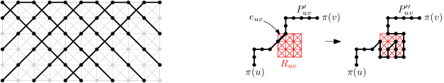
Figure 1: A large clique minor in a 2-dimensional grid with diagonals (left), and a way to increase the lengths of the path $P_{uv}^{\prime}$ using the private areas $R_{uv}$ (right).

For an odd integer $\lambda\geqslant 1$, a $\lambda$-refinement of the grid $H$ is obtained by replacing each $(1\times 1)$-cell of the grid $H$ by a $(\lambda\times\lambda)$-grid. Note that if $H$ contains a subdivision of $G$ as above, then any $\lambda$-refinement of $H$ contains a subdivision of $G$, where each path $P_{uv}$ is replaced by a path $P_{uv}^{\prime}$ of length $\lambda|P_{uv}|$. Note that after performing a $\lambda$-refinement and adding small perturbations to some of the paths $P_{uv}^{\prime}$, we can assume in addition that there is an integer $s\geqslant\lambda/2$ such that for any edge $uv$ of $G$, $H$ contains a $(s\times s)$-subgrid $R_{uv}$ that intersects the subdivision of $G$ in $H$ in a single edge $e_{uv}$, which is included in $P_{uv}^{\prime}$ (see Figure 1, right).

Using the subgrid $R_{uv}$, we can replace $e_{uv}$ by a path of any length between 1 and $(\tfrac{\lambda}{2}-1)^{2}\geqslant\lambda^{2}/16$ (assuming $\lambda\geqslant 4$) between its endpoints, turning $P_{uv}^{\prime}$ into a new path $P_{uv}^{\prime\prime}$ of length $|P_{uv}^{\prime}|+\ell=\lambda|P_{uv}|+\ell$ (for any possible value of $0\leqslant\ell\leqslant\lambda^{2}/16$), in such a way that the vertices $\pi(u)$, $u\in V(G)$, and the paths $P_{uv}^{\prime\prime}$, $uv\in E(H)$, still form a subdivision of $G$ in $H$.

Note that a path $P_{uv}$ of maximum length can replaced by a path $P_{uv}^{\prime\prime}$ of length $\lambda|P_{uv}|$ after the $\lambda$-refinement, while a path $P_{xy}$ of minimum length can be replaced by a path $P_{xy}^{\prime\prime}$ of any length between $\lambda|P_{xy}|$ and $\lambda|P_{xy}|+\lambda^{2}/16\geqslant\lambda|P_{uv}|$, where the inequality holds whenever $\lambda\geqslant 16|P_{uv}|-16|P_{xy}|$. It follows that by taking $\lambda$ sufficiently large, we obtain a subdivision of $G$ in $H$ where all edges of $G$ correspond to paths of the same length in $H$, as desired. ∎

Using a similar argument to the above, we obtain a similar result for subgraphs of 3-dimensional grids. Write ${\mathcal{P}}^{3}$ for the class of subgraphs of the 3-dimensional grid; i.e. the class of finite subgraphs of the Cartesian product $P^{3}$, where $P$ is the infinite path. We omit this proof due to its similarity to the one above.

Lemma 5.10.

For any graph $G$ of maximum degree 3, there exists a constant $k=k_{G}$ such that ${\mathcal{P}}^{3}$ contains the $k$-subdivision of $G$.

We easily deduce the following simple corollary.

Corollary 5.11.

The classes $\mathcal{G}_{2}$ and ${\mathcal{P}}^{3}$ are not ADT sketchable.

Proof.

The proof is similar to that of Theorem 5.7. Suppose for contradiction that, for some constant $\alpha>1$, the class admits a constant-size $\alpha$-approximate distance sketch. Then by Proposition 5.1, we can assume that the sketch is distance-invariant. By Lemma 5.9, this can be used to design an $\alpha$-approximate distance sketch for the class of all graphs of maximum degree 3, contradicting Theorem 5.6. ∎

5.4 Lower Bound for Classes of Low Expansion

Now we show that there is no non-constant bound on the expansion that guarantees the existence of constant-size ADT sketches. We achieve this by constructing classes of graphs of arbitrarily low non-constant expansion, which cannot admit constant-size $\alpha$-ADT sketches for any constant $\alpha>1$. We start with a simple variant of [GKR⁺18, Theorem 4.5].

For a function $f:\mathbb{N}\to\mathbb{N}$ such that $f(n)\to\infty$ when $n\to\infty$, we define $f^{-1}(n):=\max\{k\,|\,f(k)\leqslant n\}$. We recall that for an $N$-vertex graph $G$ and an integer $\ell\geqslant 2\log N+1$, the graph $G[\ell]$ was defined just before the statement of Theorem 5.6.

Lemma 5.12.

Let $f$ be a function such that $f(n)\to\infty$ when $n\to\infty$. For any $n$-vertex graph $G$, and any integer $r\geqslant 0$, every depth-$r$ minor of $G[6f(6n^{2})+2\log n]$ has average degree at most $\max\{4,f^{-1}(r)\}$.

Proof.

Let $H=G[6f(6n^{2})+2\log n]$, and let $H^{\prime}$ be any depth-$r$ minor of $H$. Observe that $G[2\log n+1]$ has at most $2n^{2}+{n\choose 2}\leqslant 3n^{2}$ vertices, and thus tree-width at most $3n^{2}$. The graph $H$ itself is obtained from $G[2\log n+1]$ by subdividing some edges, an operation that leaves the tree-width unchanged. It follows that $H$ also has tree-width at most $3n^{2}$. Since tree-width is a minor-monotone parameter, $H^{\prime}$ also has tree-width at most $3n^{2}$ and is thus $3n^{2}$-degenerate. It follows that $H^{\prime}$ has average degree at most $6n^{2}$. If $r\geqslant f(6n^{2})$, then $6n^{2}\leqslant f^{-1}(r)$ and thus $H^{\prime}$ has average degree at most $f^{-1}(r)$, as desired. Assume now that $r\leqslant f(6n^{2})$. In this case, since $H^{\prime}$ is obtained from disjoint trees by connecting their leaves with paths of length at least $6f(6n^{2})$, it can be checked that $H^{\prime}$ is 2-degenerate, and thus has average degree at most 4. ∎

Theorem 5.13.

For any function $\rho$ tending to infinity, there exists a monotone class of expansion $r\mapsto\rho(r)$ that is not ADT sketchable. Moreover, for any $\varepsilon>0$, there exists a monotone class ${\mathcal{F}}$ of expansion $r\mapsto O(r^{\varepsilon})$, such that, if ${\mathcal{F}}$ admits an $\alpha$-ADT sketch of size $s(n)$, then we must have $s(n)=n^{\Omega(1/\alpha)}$.

Proof.

Let $\rho:{\mathbb{N}}\to{\mathbb{N}}$ be a function tending to infinity, so that $\rho^{-1}$ is a non-decreasing function tending to infinity. We proceed as in the proof of Theorem 5.6, setting $\ell(N)=6\rho^{-1}(6N^{2})+2\log N$ (instead of $\ell=\lceil 4\log N\rceil$). For any $N$-vertex graph $G$, $G[\ell(N)]\in{\mathcal{F}}_{n,3}$ with $n\leqslant 6N^{2}(\rho^{-1}(6N^{2})+2\log N)$. By Lemma 5.12, any depth-$r$ minor of such a graph $G[\ell(N)]$ has average degree at most $\max\{4,\rho(r)\}$. It follows that the monotone class ${\mathcal{F}}$ of all graphs $G[\ell(N)]$ for $G\in{\mathfrak{G}}_{N}$ and their subgraphs has expansion at most $r\mapsto\max\{4,\rho(r)\}$.

By the same argument as in Theorem 5.6, if there is a distance-invariant $\alpha$-ADT sketch for ${\mathcal{F}}$ of size $s(n)$ (which is a non-decreasing function in $n$), we obtain a $(1,2\alpha)$-distance sketch for ${\mathfrak{G}}$ of size $N\mapsto s(n)$. Then, due to Corollary 5.5,

$$N^{\tfrac{1}{2\alpha}}/\log N=O\left(s(n)\right)=O\left(s\left(6N^{2}(\rho^{-1}(6N^{2})+2\log N)\right)\right)\,.$$

It is clear that, for any choice of $\rho$, we cannot have $s(n)$ constant, which establishes the first part of the theorem. To get the second part, let $\varepsilon>0$ and suppose that we choose $\rho(r)=r^{\varepsilon}$ so that $\rho^{-1}(r)=r^{1/\varepsilon}$, and assume for contradiction that $s(n)=n^{o(1/\alpha)}$. Then

$$N^{\tfrac{1}{2\alpha}}/\log N=O\left(s\left(6N^{2}((6N^{2})^{1/\varepsilon}+2\log N)\right)\right)=O\left(N^{o(1/\alpha)}\right)\,,$$

which means we must have $s(n)=n^{\Omega(1/\alpha)}$ as desired. ∎

5.5 Upper Bounds

The weak diameter of a subset $S$ of vertices of a graph $G$ is the maximum distance in $G$ between two vertices of $S$. Given a graph $G$, a $(\sigma,\tau,\Delta)$-sparse cover is a family $\mathcal{C}$ of subsets of $V(G)$ of weak diameter at most $\Delta$, such that (i) for each $u\in V(G)$, there is a set $C\in\mathcal{C}$ such that $B(u,\tfrac{\Delta}{\sigma})\subseteq C$ (where $B(u,r)$ denotes the ball of radius $r$ centered in $u$), and (ii) each vertex $u\in V(G)$ lies in at most $\tau$ sets of $\mathcal{C}$.

We say that a graph $G$ admits a $(\sigma,\tau)$-sparse cover scheme if for any $\Delta$, it admits a $(\sigma,\tau,\Delta)$-sparse cover. We say that a graph class ${\mathcal{F}}$ has a $(\sigma,\tau)$-sparse cover scheme if any graph of ${\mathcal{F}}$ has such a scheme). Classes of graphs with $(\sigma,\tau)$-sparse cover schemes are also known as classes of Assouad-Nagata dimension at most $\tau-1$ in metric geometry [Ass82] (see also [LS05]).

We recall that disjunctive labelling schemes have been defined in Subsection 2.3, and that by Proposition 2.3 they can be turned into constant-size sketches with one-sided error. The following result is a simple consequence of the definition of sparse covers. Note that here the size of the labels is independent of $r$, in contrast with the setting of Theorem 4.10 and its corollaries.

Theorem 5.14.

If a graph class ${\mathcal{F}}$ has a $(\sigma,\tau)$-sparse cover scheme, then $\mathcal{F}$ has distance-invariant, disjunctive $\sigma$-ADT labelling scheme with labels of size $O(\tau)$.

Proof.

By the definition of sparse covers, for any $r>0$, there is a family $\mathcal{C}$ of subsets of $V(G)$ of weak diameter at most $\sigma r$, such that (i) for each $u\in V(G)$, there is a set $C\in\mathcal{C}$ such that $B(u,r)\subseteq C$, and (ii) each vertex $u\in V(G)$ lies in at most $\tau$ sets of $\mathcal{C}$.

We may now define a disjunctive $\sigma$-ADT labelling scheme. Assign each set $C\in\mathcal{C}$ a unique number in ${\mathbb{N}}$, and for each vertex $x$, let $S(x)$ be the set of names of the (at most $\tau$) sets $C$ containing $x$. For each vertex $x\in V(G)$, the equality code $\vec{q}(x)$ contains the names $S(x)$, and we assign $x$ the label $(-\mid\vec{q}(x))$. On inputs $(-\mid\vec{q}(x))$ and $(-\mid\vec{q}(y))$, the decoder outputs 1 if and only $S(x)\cap S(y)\neq\emptyset$ (which can be checked using the equality codes).

Suppose $\mathsf{dist}_{G}(x,y)\leqslant r$. Since there is a set $C\in\mathcal{C}$ such that $B(x,r)\subseteq C$, we also have $y\in C$, and thus $S(x)\cap S(y)\neq\emptyset$. Now suppose that $\mathsf{dist}_{G}(x,y)>\sigma r$. Since each set $C\in\mathcal{C}$ has weak diameter at most $\sigma r$, there is no set $C\in\mathcal{C}$ containing both $x$ and $y$ and thus $S(x)\cap S(y)=\emptyset$. ∎

Using Proposition 2.3 together with results of [Fil20] on sparse covers (based on [KPR93, FT03]), we deduce the following immediate corollary.

Corollary 5.15.

For any $t\geqslant 4$, the class of $K_{t}$-minor free graphs has a distance-invariant $O(2^{t})$-ADT sketch of size $O(t^{2}\log t)$.

5.5.1 Padded Decompositions

We will see now how to obtain improved sketches using padded decompositions. These improved sketches have some disadvantages: they have two-sided error whereas the other sketches in this paper have one-sided error, and they are not equality-based. For a graph $G$, a probability distribution $\mathcal{P}$ over partitions of $V(G)$ is said to be $(\beta,\delta,\Delta)$-padded if

• for each partition $P$ in the support of $\mathcal{P}$, each set of $P$ has weak diameter at most $\Delta$, and

• for any $u\in V(G)$ and any $0\leqslant\gamma\leqslant\delta$, the ball $B(u,\gamma\Delta)$ is included in some set of a random partition from $\mathcal{P}$ with probability at least $2^{-\beta\gamma}$.

We say that a graph $G$ admits a $(\beta,\delta)$-padded decomposition scheme if for any $\Delta$, it admits a $(\beta,\delta,\Delta)$-padded distribution over partitions of $V(G)$. We say that a graph class ${\mathcal{F}}$ has a $(\beta,\delta)$-padded decomposition scheme if any graph of ${\mathcal{F}}$ has such a scheme. We note that padded decomposition schemes are incomparable with the sparse cover schemes introduced above.

Theorem 5.16.

If a graph class ${\mathcal{F}}$ has a $(\beta,\delta)$-padded decomposition scheme, then ${\mathcal{F}}$ admits a distance-invariant $\alpha$-ADT sketch of size 2, where $\alpha=\max(\tfrac{1}{\delta},\tfrac{\beta}{\log(3/2)})$.

Proof.

Fix some $r>0$, and some graph $G\in{\mathcal{F}}$. Let $\gamma=\min(\delta,\tfrac{1}{\beta}\log(3/2))$. Note that $0\leqslant\gamma\leqslant\delta$ and $2^{-\beta\gamma}\geqslant\tfrac{2}{3}$. Let $\Delta=r/\gamma$, and let $\mathcal{P}$ be a $(\beta,\delta,\Delta)$-padded distribution over partitions of $V(G)$. Let $\mathbf{P}$ be a partition of $V(G)$ drawn according to the distribution $\mathcal{P}$. Then each set of $\mathbf{P}$ has weak diameter at most $\Delta$. Assign a random identifier $\text{id}(S)$ to each set $S\in\mathbf{P}$, drawn uniformly at random from the set $\{1,2,3\}$ (each $\text{id}(S)$ requires only 2 bits). The label of each vertex $u\in V(G)$ simply consists of the identifier $\text{id}(S)$ of the unique set $S\in\mathbf{P}$ such that $u\in S$. Given the labels of $u$ and $v$, the decoder outputs 1 if and only the labels are equal. Note that the decoder is clearly distance-invariant.

Assume first that $d(u,v)\leqslant r$, then since $v$ is in the ball of radius $r=\gamma\Delta$ centered in $u$, it follows that $u$ and $v$ are in the same set $S\in\mathbf{P}$ with probability at least $2^{-\beta\gamma}\geqslant\tfrac{2}{3}$. If $u$ and $v$ are in the same set $S\in\mathbf{P}$, then their labels are equal with probability 1. It follows that if $d(u,v)\leqslant r$, the decoder outputs 1 with probability at least $2/3$, as desired.

Assume now that $d(u,v)>r/\gamma$. Since each set in $\mathbf{P}$ has weak diameter at most $\Delta=r/\gamma$, it follows that $u$ and $v$ are in different sets of $\mathbf{P}$ with probability 1. As each set $S\in\mathbf{P}$ is assigned a random element from $\{1,2,3\}$, $u$ and $v$ have the same label with probability $\tfrac{1}{3}$. It follows that if $d(u,v)>r/\gamma$, the decoder outputs 0 with probability $1-\tfrac{1}{3}=\tfrac{2}{3}$, as desired. ∎

Although this sketch does use randomization for an equality check, it also uses randomization to construct the padded decomposition, and so it is not equality-based.

It was proved in [AGG⁺19] that for $t\geqslant 4$, the class of $K_{t}$-minor free graphs admits a $(320t,\tfrac{1}{160})$-padded decomposition scheme. It was also proved in [LS10] (see also [AGG⁺19]) that for any $g\geqslant 0$, the class of graphs embeddable on a surface of Euler genus $g$ admits a $(O(\log g),\Omega(1))$-padded decomposition scheme. We obtain the following two corollaries, and again emphasize that these sketches have two-sided error.

Corollary 5.17.

For any $t\geqslant 4$, the class of $K_{t}$-minor free graphs has a distance-invariant $O(t)$-ADT sketch with labels of at most 2 bits.

Corollary 5.18.

For any $g\geqslant 0$, the class of graphs embeddable on a surface of Euler genus $g$ has a distance-invariant $O(\log g)$-ADT sketch with labels of at most 2 bits.

We remark that lower bounds for sketching therefore imply lower bounds on sparse covers and padded decompositions. For example, the communication complexity lower bound of [AK08] implies that bounded-degree expanders do not admit padded covers or sparse covers, which is something that we were unable to prove directly.

Acknowledgments.

We thank Gwenaël Joret for many helpful discussions, and for allowing us to include his proof of Theorem 4.19. We thank Viktor Zamaraev for leading us to Corollary 3.6 and carefully proofreading our manuscript. We thank Alexandr Andoni for a helpful discussion and for sharing with us the manuscript [AK08]. We thank Renato Ferreira Pinto Jr. and Sebastian Wild for comments on the presentation of this article. Finally, we thank the anonymous reviewers of the journal and conference [EHK22] versions of this paper for the many insightful comments and suggestions. We especially thank a reviewer for suggesting the simplified and improved version of Lemma 3.3.

References

- [ABR05] Stephen Alstrup, Philip Bille, and Theis Rauhe. Labeling schemes for small distances in trees. SIAM Journal on Discrete Mathematics, 19(2):448–462, 2005.
- [ACG12] Ittai Abraham, Shiri Chechik, and Cyril Gavoille. Fully dynamic approximate distance oracles for planar graphs via forbidden-set distance labels. In Proceedings, ACM Symposium on Theory of Computing (STOC 2012), pages 1199–1218, 2012.
- [ADKP16] Stephen Alstrup, Søren Dahlgaard, Mathias Bæk Tejs Knudsen, and Ely Porat. Sublinear distance labeling. In Proceedings, European Symposium on Algorithms (ESA 2016). Schloss Dagstuhl-Leibniz-Zentrum für Informatik, 2016.
- [AG06] Ittai Abraham and Cyril Gavoille. Object location using path separators. In Proceedings of the twenty-fifth annual ACM Symposium on Principles of Distributed Computing (PODC 2006), pages 188–197, 2006.
- [AGG+19] Ittai Abraham, Cyril Gavoille, Anupam Gupta, Ofer Neiman, and Kunal Talwar. Cops, robbers, and threatening skeletons: Padded decomposition for minor-free graphs. SIAM Journal on Computing, 48(3):1120–1145, 2019.
- [AGHP16a] Stephen Alstrup, Cyril Gavoille, Esben Bistrup Halvorsen, and Holger Petersen. Simpler, faster and shorter labels for distances in graphs. In Proceedings, ACM-SIAM Symposium on Discrete Algorithms (SODA 2016), pages 338–350. SIAM, 2016.
- [AGHP16b] Stephen Alstrup, Inge Li Gørtz, Esben Bistrup Halvorsen, and Ely Porat. Distance labeling schemes for trees. In Proceedings, International Colloquium on Automata, Languages, and Programming (ICALP 2016). Schloss Dagstuhl-Leibniz-Zentrum für Informatik, 2016.
- [AK08] Alexandr Andoni and Robert Krauthgamer. Distance estimation protocols for general metrics. https://www.cs.columbia.edu/~andoni/papers/de.pdf, 2008.
- [AKR18] Alexandr Andoni, Robert Krauthgamer, and Ilya P. Razenshteyn. Sketching and embedding are equivalent for norms. SIAM J. Comput., 47(3):890–916, 2018.
- [AMS99] Noga Alon, Yossi Matias, and Mario Szegedy. The space complexity of approximating the frequency moments. Journal of Computer and system sciences, 58(1):137–147, 1999.
- [AP90] Baruch Awerbuch and David Peleg. Sparse partitions (extended abstract). In Proceedings, Symposium on Foundations of Computer Science (FOCS 1990), pages 503–513. IEEE, 1990.
- [Ass82] Patrice Assouad. Sur la distance de Nagata. CR Acad. Paris, 294:31–34, 1982.
- [AY22] Daniel Avraham and Amir Yehudayoff. On block ranks of matrices. Electronic Colloquium on Computational Complexity (ECCC), page 137, 2022.
- [BBM+21] Alexander R. Block, Simina Brânzei, Hemanta K. Maji, Himanshi Mehta, Tamalika Mukherjee, and Hai H. Nguyen. -free Partition and Cover Numbers & Applications. In Proceedings, Conference on Information-Theoretic Cryptography (ITC 2021). Schloss Dagstuhl – Leibniz-Zentrum für Informatik, 2021.
- [BGK+21] Édouard Bonnet, Colin Geniet, Eun Jung Kim, Stéphan Thomassé, and Rémi Watrigant. Twin-width II: small classes. In Proceedings, ACM-SIAM Symposium on Discrete Algorithms (SODA 2021), pages 1977–1996. SIAM, 2021.
- [CHZZ22] Tsun-Ming Cheung, Hamed Hatami, Rosie Zhao, and Itai Zilberstein. Boolean functions with small approximate spectral norm. Electronic Colloquium on Computational Complexity (ECCC), 2022. TR22-041.
- [CLR20] Victor Chepoi, Arnaud Labourel, and Sébastien Ratel. On density of subgraphs of Cartesian products. Journal of Graph Theory, 93(1):64–87, 2020.
- [CLV19] Arkadev Chattopadhyay, Shachar Lovett, and Marc Vinyals. Equality alone does not simulate randomness. In Proceedings, Computational Complexity Conference (CCC 2019). Schloss Dagstuhl-Leibniz-Zentrum für Informatik, 2019.
- [DJM+20] Vida Dujmovic, Gwenaël Joret, Piotr Micek, Pat Morin, Torsten Ueckerdt, and David R. Wood. Planar graphs have bounded queue-number. J. ACM, 67(4):22:1–22:38, 2020.
- [DMW17] Vida Dujmović, Pat Morin, and David R. Wood. Layered separators in minor-closed graph classes with applications. J. Comb. Theory, Ser. B, 127:111–147, 2017.
- [DN16] Zdeněk Dvorák and Sergey Norin. Strongly sublinear separators and polynomial expansion. SIAM J. Discret. Math., 30(2):1095–1101, 2016.
- [DRR+14] Erik D. Demaine, Felix Reidl, Peter Rossmanith, Fernando Sánchez Villaamil, Somnath Sikdar, and Blair D Sullivan. Structural sparsity of complex networks: Bounded expansion in random models and real-world graphs. arXiv preprint arXiv:1406.2587, 2014.
- [Dvo08] Zdeněk Dvorák. On forbidden subdivision characterizations of graph classes. European J. Combin., 29(5):1321–1332, 2008.
- [Dvo21] Zdeněk Dvorák. A note on sublinear separators and expansion. European J. Combin., 93:103273, 2021.
- [Dvo23] Zdenek Dvorák. Representation of short distances in structurally sparse graphs. In Proceedings, International Symposium on Theoretical Aspects of Computer Science (STACS 2023). Schloss Dagstuhl - Leibniz-Zentrum für Informatik, 2023.
- [EHK22] Louis Esperet, Nathaniel Harms, and Andrey Kupavskii. Sketching Distances in Monotone Graph Classes. In Proceedings of Approximation, Randomization, and Combinatorial Optimization. Algorithms and Techniques (APPROX/RANDOM 2022), pages 18:1–18:23. Schloss Dagstuhl – Leibniz-Zentrum für Informatik, 2022.
- [EHZ23] Louis Esperet, Nathaniel Harms, and Viktor Zamaraev. Optimal adjacency labels for subgraphs of cartesian products. In Proceedings, International Colloquium on Automata, Languages, and Programming (ICALP 2023). Schloss Dagstuhl - Leibniz-Zentrum für Informatik, 2023.
- [EIX22] Talya Eden, Piotr Indyk, and Haike Xu. Embeddings and labeling schemes for . In Proceedings, Innovations in Theoretical Computer Science Conference (ITCS 2022). Schloss Dagstuhl–Leibniz-Zentrum für Informatik, 2022.
- [Epp00] David Eppstein. Diameter and treewidth in minor-closed graph families. Algorithmica, 27(3):275–291, 2000.
- [FGNW17] Ofer Freedman, Paweł Gawrychowski, Patrick K. Nicholson, and Oren Weimann. Optimal distance labeling schemes for trees. In Proceedings, ACM Symposium on Principles of Distributed Computing (PODC 2017), pages 185–194, 2017.
- [FHL+23] Irene Gil Fernández, Joseph Hyde, Hong Liu, Oleg Pikhurko, and Zhuo Wu. Disjoint isomorphic balanced clique subdivisions. Journal of Combinatorial Theory, Series B, 161:417–436, 2023.
- [Fil20] Arnold Filtser. Scattering and sparse partitions, and their applications. In Proceedings, International Colloquium on Automata, Languages, and Programming (ICALP 2020). Schloss Dagstuhl-Leibniz-Zentrum für Informatik, 2020.
- [FK09] Pierre Fraigniaud and Amos Korman. On randomized representations of graphs using short labels. In Proceedings, Symposium on Parallelism in Algorithms and Architectures (SPAA 2009), pages 131–137, 2009.
- [FT03] Jittat Fakcharoenphol and Kunal Talwar. An improved decomposition theorem for graphs excluding a fixed minor. In Proceedings of Approximation, Randomization, and Combinatorial Optimization: Algorithms and Techniques (APPROX/RANDOM 2003), pages 36–46. Springer, 2003.
- [GHN+12] Robert Ganian, Petr Hlinený, Jaroslav Nešetřil, Jan Obdrzálek, Patrice Ossona de Mendez, and Reshma Ramadurai. When trees grow low: Shrubs and fast MSO1. In Branislav Rovan, Vladimiro Sassone, and Peter Widmayer, editors, Mathematical Foundations of Computer Science 2012 - 37th International Symposium, MFCS 2012, Bratislava, Slovakia, August 27-31, 2012. Proceedings, volume 7464 of Lecture Notes in Computer Science, pages 419–430. Springer, 2012.
- [GHN+19] Robert Ganian, Petr Hlinený, Jaroslav Nešetřil, Jan Obdrzálek, and Patrice Ossona de Mendez. Shrub-depth: Capturing height of dense graphs. Log. Methods Comput. Sci., 15(1), 2019.
- [GKK+01] Cyril Gavoille, Michal Katz, Nir A. Katz, Christophe Paul, and David Peleg. Approximate distance labeling schemes. In Proceedings, European Symposium on Algorithms (ESA 2001), pages 476–487. Springer, 2001.
- [GKN+20] Jakub Gajarský, Stephan Kreutzer, Jaroslav Nešetřil, Patrice Ossona de Mendez, Michał Pilipczuk, Sebastian Siebertz, and Szymon Toruńczyk. First-order interpretations of bounded expansion classes. ACM Trans. Comput. Logic, 21(4), jul 2020.
- [GKR+18] Martin Grohe, Stephan Kreutzer, Roman Rabinovich, Sebastian Siebertz, and Konstantinos Stavropoulos. Coloring and covering nowhere dense graphs. SIAM Journal on Discrete Mathematics, 32(4):2467–2481, 2018.
- [GKS17] Martin Grohe, Stephan Kreutzer, and Sebastian Siebertz. Deciding first-order properties of nowhere dense graphs. Journal of the ACM (JACM), 64(3):1–32, 2017.
- [GL07] Cyril Gavoille and Arnaud Labourel. On local representation of distances in trees. In Proceedings, ACM Symposium on Principles of Distributed Computing (PODC 2007), pages 352–353, 2007.
- [GNRS04] Anupam Gupta, Ilan Newman, Yuri Rabinovich, and Alistair Sinclair. Cuts, trees and -embeddings of graphs. Combinatorica, 24(2):233–269, 2004.
- [GP03] Cyril Gavoille and David Peleg. Compact and localized distributed data structures. Distributed Computing, 16(2):111–120, 2003.
- [GPPR04] Cyril Gavoille, David Peleg, Stéphane Pérennes, and Ran Raz. Distance labeling in graphs. Journal of Algorithms, 53(1):85–112, 2004.
- [GPT22] Jakub Gajarský, Michal Pilipczuk, and Szymon Torunczyk. Stable graphs of bounded twin-width. In Proceedings, ACM/IEEE Symposium on Logic in Computer Science (LICS 2022), pages 39:1–39:12. ACM, 2022.
- [GPW18] Mika Göös, Toniann Pitassi, and Thomas Watson. The landscape of communication complexity classes. Computational Complexity, 27:245–304, 2018.
- [Gra70] Ron L. Graham. On primitive graphs and optimal vertex assignments. Annals of the New York academy of sciences, 175(1):170–186, 1970.
- [GU21] Paweł Gawrychowski and Przemysław Uznański. Better distance labeling for unweighted planar graphs. In Workshop on Algorithms and Data Structures (WADS 2021), pages 428–441. Springer, 2021.
- [Har20] Nathaniel Harms. Universal communication, universal graphs, and graph labeling. In Proceedings, Innovations in Theoretical Computer Science Conference (ITCS 2020), page 33. Schloss Dagstuhl–Leibniz-Zentrum für Informatik, 2020.
- [Har22] Nathaniel Harms. Adjacency labeling and sketching for induced subgraphs of the hypercube. https://cs.uwaterloo.ca/~nharms/downloads/hypercube_sketch.pdf, 2022.
- [HH22] Hamed Hatami and Pooya Hatami. The implicit graph conjecture is false. In Proceedings, IEEE Annual Symposium on Foundations of Computer Science (FOCS 2022), pages 1134–1137. IEEE, 2022.
- [HHH22] Lianna Hambardzumyan, Hamed Hatami, and Pooya Hatami. A counter-example to the probabilistic universal graph conjecture via randomized communication complexity. Discret. Appl. Math., 322:117–122, 2022.
- [HHH23] Lianna Hambardzumyan, Hamed Hatami, and Pooya Hatami. Dimension-free bounds and structural results in communication complexity. Isr. J. Math., 253(2):555–616, 2023.
- [HHM23] Hamed Hatami, Kaave Hosseini, and Xiang Meng. A Borsuk-Ulam lower bound for sign-rank and its applications. In Barna Saha and Rocco A. Servedio, editors, Proceedings, ACM Symposium on Theory of Computing, (STOC 2023), pages 463–471. ACM, 2023.
- [HHP+22] Hamed Hatami, Pooya Hatami, William Pires, Ran Tao, and Rosie Zhao. Lower bound methods for sign-rank and their limitations. In Proceedings of Approximation, Randomization, and Combinatorial Optimization. Algorithms and Techniques (RANDOM 2022). Schloss Dagstuhl-Leibniz-Zentrum für Informatik, 2022.
- [HMŠ+21] Tony Huynh, Bojan Mohar, Robert Šámal, Carsten Thomassen, and David R Wood. Universality in minor-closed graph classes. arXiv preprint arXiv:2109.00327, 2021.
- [HSZZ06] Wei Huang, Yaoyun Shi, Shengyu Zhang, and Yufan Zhu. The communication complexity of the hamming distance problem. Information Processing Letters, 99(4):149–153, 2006.
- [HWZ22] Nathaniel Harms, Sebastian Wild, and Viktor Zamaraev. Randomized communication and implicit graph representations. In Proceedings, ACM Symposium on Theory of Computing (STOC 2022), 2022.
- [IM98] Piotr Indyk and Rajeev Motwani. Approximate nearest neighbors: towards removing the curse of dimensionality. In Proceedings, ACM Symposium on Theory of Computing (STOC 1998), pages 604–613, 1998.
- [Ind06] Piotr Indyk. Stable distributions, pseudorandom generators, embeddings, and data stream computation. Journal of the ACM (JACM), 53(3):307–323, 2006.
- [Jay09] T.S. Jayram. Problem 25: Communication complexity and metric spaces. https://sublinear.info/25, 2009.
- [KN19] Subhash Khot and Assaf Naor. The Andoni–Krauthgamer–Razenshteyn characterization of sketchable norms fails for sketchable metrics. In Proceedings, ACM-SIAM Symposium on Discrete Algorithms (SODA 2019), pages 1814–1824. SIAM, 2019.
- [KNR92] Sampath Kannan, Moni Naor, and Steven Rudich. Implicit representation of graphs. SIAM Journal on Discrete Mathematics, 5(4):596–603, 1992.
- [KO04] Daniela Kühn and Deryk Osthus. Every graph of sufficiently large average degree contains a -free subgraph of large average degree. Combinatorica, 24(1):155–162, 2004.
- [KOR00] Eyal Kushilevitz, Rafail Ostrovsky, and Yuval Rabani. Efficient search for approximate nearest neighbor in high dimensional spaces. SIAM Journal on Computing, 30(2):457–474, 2000.
- [KPR93] Philip Klein, Serge A. Plotkin, and Satish Rao. Excluded minors, network decomposition, and multicommodity flow. In Proceedings, ACM Symposium on Theory of Computing (STOC 1993), pages 682–690, 1993.
- [LM20] Hong Liu and Richard Montgomery. A solution to Erdős and Hajnal’s odd cycle problem. arXiv preprint arXiv:2010.15802, 2020.
- [LS05] Urs Lang and Thilo Schlichenmaier. Nagata dimension, quasisymmetric embeddings, and lipschitz extensions. International Mathematics Research Notices, 2005(58):3625–3655, 2005.
- [LS10] James R. Lee and Anastasios Sidiropoulos. Genus and the geometry of the cut graph. In Proceedings, ACM-SIAM Symposium on Discrete Algorithms (SODA 2010), pages 193–201. SIAM, 2010.
- [LTWY22] Bingyu Luan, Yantao Tang, Guanghui Wang, and Donglei Yang. Balanced subdivisions of cliques in graphs, 2022.
- [Mat96] Jiří Matoušek. On the distortion required for embedding finite metric spaces into normed spaces. Israel Journal of Mathematics, 93(1):333–344, 1996.
- [Mat13] Jiří Matoušek. Lectures on discrete geometry, volume 212. Springer Science & Business Media, 2013.
- [Mul89] John H. Muller. Local structure in graph classes. 1989.
- [NO08] Jaroslav Nešetřil and Patrice Ossona de Mendez. Grad and classes with bounded expansion II. algorithmic aspects. European Journal of Combinatorics, 29(3):777–791, 2008.
- [NO12] Jaroslav Nešetřil and Patrice Ossona de Mendez. Sparsity: graphs, structures, and algorithms, volume 28. Springer-Verlag, 2012.
- [NO15] Jaroslav Nešetřil and Patrice Ossona de Mendez. On low tree-depth decompositions. Graphs and combinatorics, 31(6):1941–1963, 2015.
- [NOdMS22] Jaroslav Nešetřil, Patrice Ossona de Mendez, and Sebastian Siebertz. Structural properties of the first-order transduction quasiorder. In Proceedings, EACSL Annual Conference on Computer Science Logic (CSL 2022). Schloss Dagstuhl-Leibniz-Zentrum für Informatik, 2022.
- [NOW12] Jaroslav Nešetřil, Patrice Ossona de Mendez, and David R. Wood. Characterisations and examples of graph classes with bounded expansion. European Journal of Combinatorics, 33(3):350–373, 2012.
- [Pel05] David Peleg. Informative labeling schemes for graphs. Theoretical Computer Science, 340(3):577–593, 2005.
- [PSS23] Toniann Pitassi, Morgan Shirley, and Adi Shraibman. The strength of equality oracles in communication. In Proceedings, Innovations in Theoretical Computer Science Conference (ITCS 2023), 2023.
- [Raz17] Ilya Razenshteyn. High-dimensional similarity search and sketching: algorithms and hardness. PhD thesis, Massachusetts Institute of Technology, 2017.
- [RS84] Neil Robertson and Paul D. Seymour. Graph minors. III. planar tree-width. Journal of Combinatorial Theory, Series B, 36(1):49–64, 1984.
- [Spi03] Jeremy P. Spinrad. Efficient graph representations. American Mathematical Society, 2003.
- [SS02] Michael Saks and Xiaodong Sun. Space lower bounds for distance approximation in the data stream model. In Proceedings, ACM Symposium on Theory of Computing (STOC 2002), pages 360–369, 2002.
- [Tho83] Carsten Thomassen. Girth in graphs. Journal of Combinatorial Theory, Series B, 35(2):129–141, 1983.
- [Tho04] Mikkel Thorup. Compact oracles for reachability and approximate distances in planar digraphs. Journal of the ACM, 51(6):993–1024, 2004.
- [TZ05] Mikkel Thorup and Uri Zwick. Approximate distance oracles. Journal of the ACM, 52(1):1–24, 2005.
- [vdHOQ+17] Jan van den Heuvel, Patrice Ossona de Mendez, Daniel Quiroz, Roman Rabinovich, and Sebastian Siebertz. On the generalised colouring numbers of graphs that exclude a fixed minor. European Journal of Combinatorics, 66:129–144, 2017.