Bjorken flow revisited: analytic and numerical solutions in flat space-time coordinates

Abstract

In this work we provide analytic and numerical solutions for the Bjorken flow, a standard benchmark in relativistic hydrodynamics providing a simple model for the bulk evolution of matter created in collisions between heavy nuclei.

We consider relativistic gases of both massive and massless particles, working in a $(2+1)$ and $(3+1)$ Minkowski space-time coordinate system. The numerical results from a recently developed lattice kinetic scheme show excellent agreement with the analytic solutions.

1 Introduction

In recent years, experimental data from the Relativistic Heavy-Ion Collider (RHIC) and the Large Hadron Collider (LHC) [1, 2, 3, 4, 5] has provided the first clear observation of the Quark-Gluon Plasma (QGP), a deconfined phase of matter where quarks and gluons are effectively free beyond the nucleonic volume [6, 7, 8].

Remarkably, the earliest stages following the heavy-ion collisions present collective behaviors that can be described by the laws of fluid dynamics [9], and indeed these results have significantly boosted the interest in the study of viscous relativistic fluid dynamics [10], both at the level of theoretical formulations as well as in the development of reliable numerical simulation methods.

Most of the numerical methods are based on Israel-Stewart theory [11] or more recent second-order causal formalism [12], with a few example represented by MUSIC [13], vSHASTA [14], ECHO-QGP [15], and several more (see e.g. [16, 17] and citations therein). Besides, mesoscopic approaches are often employed in order to study relativistic hydrodynamic systems, including lattice kinetic schemes [18], as well as Monte Carlo based methods [19, 20].

The development of new numerical tools for the study of relativistic fluids is an active field of research. However evaluating and comparing the accuracy, stability and performance of the available solvers represent a challenging task, due to the fact that numerical benchmarks with an analytic solution are rare and available only in very idealized situations.

Two of the most commonly used benchmarks are the Riemann problem [21, 22], for which an analytic solution is available only in the inviscid limit (see [23, 24, 25, 26, 27] for numerical results in the viscous regime), and the Bjorken flow [28] (as well as its generalization given by the Gubser flow [29]).

The Bjorken flow represents the simplest numerical setup in the QGP context. Under the assumption that all particles get their velocity at the initial collision, the Bjorken flow describes the boost-invariant longitudinal (i.e. along the heavy-ion beams) expansion of the QGP. Because of its formulation, this flow is naturally described recurring to the Milne coordinate system, where the macroscopic velocity results at rest. The formulation of the flow in a static Minkowski space-time is on one hand more complex, but potentially useful in the validation of codes working in a Cartesian laboratory frame coordinates.

In this work, we present the analytic solution for the Bjorken flow, considering a inviscid fluid consisting of both massive and massless particles, working in a $(2+1)$ and $(3+1)$ Minkowski space-time coordinate system.

We provide details for the implementation of the benchmark using the Relativistic Lattice Boltzmann Method (RLBM) [18], a class of numerical models providing a computational efficient approach for the solution of the the relaxation time approximation of the relativistic Boltzmann equation. Since lattice kinetic models rely on a mesoscopic description of the dynamics viscous effects are naturally included, with relativistic invariance and causality preserved by construction (this at variance with respect to aforementioned hydrodynamic models).

Numerical results are shown to be in excellent agreement with the analytic solutions.

This paper is organized as follows: in Sec. 2 we provide a brief introduction on the notation and the relevant equations for the kinetic description of a relativistic fluid. In Sec. 3 we provide analytic solutions for the Bjorken flow in a Minkowski space-time for fluids of both massive and massless particles. In Sec. 4 we report the implementation of the benchmark with RLBM, and compare the numerical results with the analytic solutions for a few selected cases.

Finally, conclusions are summarized in Sec. 5.

2 Ideal Relativistic Hydrodynamics

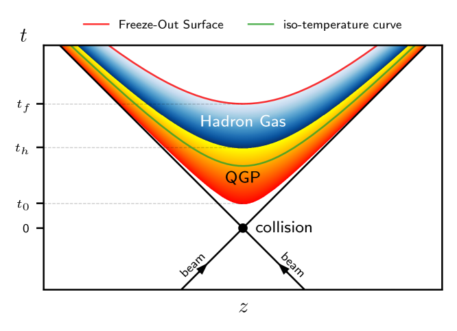
Figure 1: Schematic description of the phase transitions occurring in QGP in a z-t plane. At a time $t_{0}\sim 1$ fm/c after the collision and at values of temperature above the Hagedorn temperature, quarks become deconfined and free to roam in a so called gas of colored charges that interact with each other through the strong force. The resulting QGP fireball expands and cools down until hadronization becomes possible again ($t_{h}\sim 5$ fm/c), and the QGP quickly turns into a gas of hadrons that undergoes further transformations as neutrons and protons aggregate into nuclei (chemical freeze-out) and later on nuclei and electrons aggregate into atoms (thermal freeze out, occurring at time $t=t_{f}$). This point corresponds in the history of the Universe to the surface of last scattering, when Cosmic Microwave Background was formed.

In this section we consider a gas of particles with rest mass $m$ in a (d+1)-dimensional Minkowski space-time. The metric tensor is given by $\eta^{\alpha\beta}=\text{diag}(1,-\mathds{1})$, with $\mathds{1}=\left(1,\dots,1\right)\in\mathbb{N}^{d}$.

Einstein’s summation convention is in place, with Greek indexes running from $0$ to $d$, and latin indexes running from $1$ to $d$ (spatial d-dimensional vectors are represented in bold).

The starting point in the development of a relativistic kinetic theory is the single-particle distribution function $f(x^{\alpha},p^{\alpha})$, where $x^{\alpha}=(ct,\bm{x})$ are space-time coordinates, and $p^{\alpha}=(p^{0},\bm{p})$ is relativistic momentum, that accounts for the number of particles contained at time $t$ in the $2d$-dimensional phase space of infinitesimal volume $d\bm{x}d\bm{p}$.

An evolution equation for $f(x^{\alpha},p^{\alpha})$ can be worked out considering the usual hypothesis of kinetic theory and the language of special relativity:

$$p^{\alpha}\frac{\partial f}{\partial x^{\alpha}}=-\frac{p^{\alpha}U_{\alpha}}{c^{2}\tau}\big{(}f-f^{\mbox{\tiny eq}}\big{)}\;,$$ (1)

the so called Relativistic Boltzmann Equation, here written in the Anderson-Witting approximation [30]. $\tau$ is a typical relaxation time, i.e. the typical time needed to $f$ to approach its equilibrium value $f^{\mbox{\tiny eq}}$, the Maxwell-Jüttner  [31] distribution

$$f^{\mbox{\tiny eq}}=\left(\frac{c}{k_{\rm B}T}\right)^{d}\frac{n}{2^{\frac{d+1}{2}}\pi^{\frac{d-1}{2}}\zeta^{\frac{d+1}{2}}K_{\frac{d+1}{2}}(\zeta)}exp{\left(-\frac{p^{\alpha}U_{\alpha}}{k_{\rm B}T}\right)}\;,$$ (2)

where $K_{i}(\zeta)$ is the modified Bessel function of the second kind of index $i$, $T(\bm{x},t)$ the temperature, $n(\bm{x},t)$ the particle number density, $U^{\alpha}(\bm{x},t)$ the macroscopic fluid velocity.

The parameter $\zeta=\frac{mc^{2}}{k_{\rm B}T}$, named Relativistic Coldness, is the ratio between the rest energy of a particle $mc^{2}$ and the thermal energy of the gas $k_{\rm B}T$. This is the parameter that quantifies the level of ’relativity’ of the gas:

$$\zeta\ll 1\quad\Rightarrow$$ ultra-relativistic regime (massless particles)

$$\zeta\sim 1\quad\Rightarrow$$ mildly-relativistic regime

$$\zeta\gg 1\quad\Rightarrow$$ classical (non-relativistic) regime

The first and second order moments of the distribution function $f(x^{\alpha},p^{\alpha})$ are the quantities of interest in relativistic hydrodynamics, the Particle Flow $N^{\alpha}$ and the Energy-Momentum Tensor $T^{\alpha\beta}$:

$$N^{\alpha} =c\int p^{\alpha}f\frac{d\bm{p}}{p^{0}}\;,$$ (3)

$$T^{\alpha\beta} =c\int p^{\alpha}p^{\beta}f\frac{d\bm{p}}{p^{0}}\;.$$ (4)

These quantities are conserved under collisions,

$$\partial_{\alpha}N^{\alpha}=0\;,\quad\quad\quad\partial_{\alpha}T^{\alpha\beta}=0\;,$$ (5)

and when the fluid is ideal they can be decomposed in the following way:

$$N^{\alpha} =nU^{\alpha}\;,$$ (6)

$$T^{\alpha\beta} =(\epsilon-P)\frac{U^{\alpha}U^{\beta}}{c^{2}}+P\eta^{\alpha\beta}\;,$$ (7)

where $P(\bm{x},t)$ is the hydrostatic pressure and $\epsilon(\bm{x},t)$ the energy density.

Lastly the following ideal Equation of State (EOS) is considered:

$$\begin{array}[]{rll}\epsilon&=&P\left(\zeta\frac{K_{\frac{d+3}{2}}(\zeta)}{K_{\frac{d+1}{2}}(\zeta)}-1\right)\;,\\ P&=&nk_{\rm B}T\;.\end{array}$$ (8)

3 Bjorken Flow

At sufficiently high energies ($k_{\rm B}T\sim 1$ GeV - $1$ TeV), quarks and gluons become asymptotically free from the strong interaction which binds them into hadrons, and form a plasma of Partons which can be thought of as an extremely dense and hot gas of relativistic particles.

The gas expands and cools down, until the hadronization temperature ($k_{\rm B}T\sim 170$ MeV, also called Hagedorn temperature [32]) is reached. Matter re-hadronize into baryons and mesons. As the temperature further decreases, the gas goes through two additional phase transitions: at $k_{\rm B}T\sim 100$ KeV protons and neutrons bind together to form atomic nuclei (Chemical Freeze-Out), and at $k_{\rm B}T\sim 1/4$ eV (Thermal Freeze-Out) complete atoms are formed.

The process here described, and sketched in Fig. 1, is expected to provide a description of the first moments after the big bang [33].

The Bjorken flow, also called the mono-dimensional boost invariant expansion model [28], represents the simplest setup for modeling the longitudinal expansion of the dynamics observed in heavy ion collisions in particle accelerators.

It takes into consideration an inviscid fluid which is expanding along the propagation direction of the two beams (the z-axis cf. Fig. 1), with fluid velocity

$$\beta=\frac{U^{z}}{U^{0}}=\frac{z}{ct}\;.$$ (9)

In the next section, we detail the governing equations of the flow, and provide details on the analytical solutions. For simplicity, in what follow we make use of natural units: $c=k_{\rm B}=1$.

3.1 Analytic Solution for an ideal fluid

We use a flat space-time, with coordinates $(t,z)$, where only the spatial coordinate $z$ is considered since it is assumed that no transverse dynamic develops.

As previously mentioned, the most natural coordinate system for describing a Bjorken flow is given by Milne coordinates, since in this metric the flow describes a static fluid in a longitudinally expanding space-time. Milne coordinates $(\uptau,w)$ are defined as

$$\begin{cases}\uptau&=\sqrt{t^{2}-z^{2}}\\ w&=\operatorname{arctanh}{\left(\frac{z}{t}\right)}\end{cases}\;.$$ (10)

In what follows, we denote with a tilde superscript quantities expressed in the Milne metric.

We define the following transformation matrix between the two reference frames:

$$\Lambda^{\mu}_{\phantom{\mu}\nu}=\frac{\partial\tilde{x}^{\mu}}{\partial x^{\nu}}\quad;$$ (11)

the above provides an expression for the metric in the new basis:

$$\tilde{\eta}^{\alpha\beta} =\Lambda_{\mu\phantom{\alpha}}^{\alpha}\Lambda_{\nu\phantom{\beta}}^{\beta}~{}\eta^{\mu\nu}=\text{diag}\left(+1,-\frac{1}{\uptau^{2}}\right)\;,$$ (12)

$$\tilde{\eta}_{\alpha\beta} =\text{diag}\left(+1,-\uptau^{2}\right)\;.$$ (13)

Moreover, the curvilinear coordinates define Christoffel symbols $\Gamma^{\alpha}_{\beta\gamma}$, and the usual derivative is replaced with the covariant derivative:

$$A^{\alpha}_{;\beta}=\partial_{\beta}A^{\alpha}+\Gamma^{\alpha}_{\beta\gamma}A^{\gamma}\;.$$ (14)

Milne’s Christoffel symbols are defined by

$$\tilde{\Gamma}^{0}_{dd}=\uptau\quad\quad\tilde{\Gamma}^{d}_{0d}=\frac{1}{\uptau}\quad\quad\tilde{\Gamma}^{d}_{d0}=\frac{1}{\uptau}\;,$$ (15)

with all the other symbols being zero.

From the condition in Eq. 9, we define the macroscopic velocity $U^{\alpha}$:

$$U^{\alpha}=\frac{1}{\sqrt{t^{2}-z^{2}}}\left(t,z\right)\;.$$ (16)

By applying the transformation matrix $\Lambda^{\mu}_{\phantom{\mu}\nu}$ we obtain the corresponding Milne macroscopic velocity $\tilde{U}^{\alpha}$:

$$\tilde{U}^{\mu}=\Lambda^{\mu}_{\phantom{\mu}\nu}U^{\nu}=(1,0)\;.$$ (17)

The particle-flow (Eq. 3) and the energy-momentum tensor (Eq. 4) in Milne coordinates write as

$$\tilde{N}^{\alpha} =n\tilde{U}^{\alpha}\;,$$ (18)

$$\tilde{T}^{\alpha\beta} =(\epsilon+P)\tilde{U}^{\alpha}\tilde{U}^{\beta}-P\tilde{\eta}^{\alpha\beta}\;.$$ (19)

Moreover, the balance equations (Eq. 5) in Milne coordinates take the form

$$0 =\tilde{N}^{\alpha}_{\phantom{\alpha};\alpha}=\partial_{\alpha}\tilde{N}^{\alpha}+\tilde{\Gamma}^{\beta}_{\beta\alpha}\tilde{N}^{\alpha}\;,$$ (20)

$$0 =\tilde{T}^{\alpha\beta}_{\phantom{\alpha\beta};\alpha}=\partial_{\alpha}\tilde{T}^{\alpha\beta}+\tilde{\Gamma}^{\beta}_{\mu\alpha}\tilde{T}^{\mu\alpha}+\tilde{\Gamma}^{\alpha}_{\mu\alpha}\tilde{T}^{\mu\beta}\;.$$ (21)

By imposing such conservation equations, in combination with Eq. 17 and Eq.  18, one gets:

$$0 =\partial_{\uptau}(n\uptau)\;,$$

$$0 =\partial_{\uptau}(\epsilon)+\frac{P+\epsilon}{\uptau}\;,$$ (22)

$$0 =\partial_{w}(P)\;,$$

Combining the above with the EOS it is possible to derive analytic expressions for the particle number density $n$, the energy density $\epsilon$, and the temperature $T$.

Considering a ultra-relativistic gas, with ideal EOS

$$P =nT\;,$$

$$\epsilon =dP\;,$$ (23)

the solution for the scalar fields $n,\epsilon,P,T$ can be obtained in the local Minkowski metric with a simple coordinate substitution, leading to:

$$n(\uptau) =n_{0}\frac{\uptau_{0}}{\uptau}=n_{0}\left(\frac{t_{0}^{2}-z_{0}^{2}}{t^{2}-z^{2}}\right)^{1/2}\;,$$

$$\epsilon(\uptau) =\epsilon_{0}\left(\frac{\uptau_{0}}{\uptau}\right)^{\frac{d+1}{d}}=\epsilon_{0}\left(\frac{t_{0}^{2}-z_{0}^{2}}{t^{2}-z^{2}}\right)^{\frac{d+1}{2d}}\;,$$ (24)

$$P(\uptau) =P_{0}\left(\frac{\uptau_{0}}{\uptau}\right)^{\frac{d+1}{d}}=P_{0}\left(\frac{t_{0}^{2}-z_{0}^{2}}{t^{2}-z^{2}}\right)^{\frac{d+1}{2d}}\;,$$

$$T(\uptau) =T_{0}\left(\frac{\uptau_{0}}{\uptau}\right)^{\frac{1}{d}}=t_{0}\left(\frac{t_{0}^{2}-z_{0}^{2}}{t^{2}-z^{2}}\right)^{\frac{1}{2d}}\;.$$

In the above, the values $(n_{0},\epsilon_{0},P_{0},T_{0})$ are prescribed at $\uptau=\uptau_{0}(t_{0},z_{0})$.

We remark that for the more general EOS in Eq. 8, suitable for a fluid consisting of massive particles $(\zeta\neq 0)$, it is necessary to perform numerical integrations of the equations in Eq. 3.1. Specifically, one takes the second of Eq. 3.1 and expresses it using the EOS Eq. 8:

$$\partial_{\tau}\left[nT\left(\zeta(T)\frac{K_{\frac{d+3}{2}}(\zeta(T))}{K_{\frac{d+1}{2}}(\zeta(T))}-1\right)\right]+\frac{nT}{\tau}\left(\zeta(T)\frac{K_{\frac{d+3}{2}}(\zeta(T))}{K_{\frac{d+1}{2}}(\zeta(T))}\right)=0\;.$$ (25)

Combining the above with the equation for the density (Eq. 3.1) delivers

$$-\frac{nT}{\tau}\left(\zeta(T)\frac{K_{\frac{d+3}{2}}(\zeta(T))}{K_{\frac{d+1}{2}}(\zeta(T))}-1\right)+n\partial_{\tau}\left[T\left(\zeta(T)\frac{K_{\frac{d+3}{2}}(\zeta(T))}{K_{\frac{d+1}{2}}(\zeta(T))}-1\right)\right]+\frac{nT}{\tau}\left(\zeta(T)\frac{K_{\frac{d+3}{2}}(\zeta(T))}{K_{\frac{d+1}{2}}(\zeta(T))}\right)=0\;,$$

from which it directly follows,

$$\partial_{\uptau}\left[T\left(\zeta(T)\frac{K_{\frac{d+3}{2}}(\zeta(T))}{K_{\frac{d+1}{2}}(\zeta(T))}-1\right)\right]+\frac{T}{\uptau}=0\;.$$ (26)

4 Numerical Results

In this section we report numerical results for the Bjorken flow simulated in a $(2+1)$ and $(3+1)$ Minkowski coordinate system, using the Relativistic Lattice Boltzmann Method (RLBM). We first give a short overview of the numerical method, followed by a comparison of the numerical results with the analytic solutions presented in the previous section.

4.1 Relativistic Lattice Boltzmann Method

RLBM is a computationally efficient approach to dissipative relativistic hydrodynamics. The derivation of the method and its algorithm (see [18] for full details), closely follow its non-relativistic counterpart [34, 35]: RLBM solves a minimal version of Eq. 1, in which the discretization of the microscopic momentum vector on a Cartesian grid is coupled with a Gauss-type quadrature which ensures the preservation of the lower (hydrodynamics) moments of the particle distribution:

$$f_{i}(\bm{x}+\bm{v}_{i}\Delta t,t+\Delta t)=f_{i}(\bm{x},t)-\Delta t\frac{p^{\mu}_{i}U^{\mu}}{cp_{i}^{0}\tau}\left(f_{i}(\bm{x},t)-f_{i}^{\rm eq}(\bm{x},t)\right)\quad i=1,2,\dots M\quad.$$ (27)

where $\bm{v}_{i}=\bm{p}_{i}/p^{0}_{i}$ are the (discrete) microscopic velocities, and $f_{i}^{\mbox{\tiny eq}}{}$ is the discrete equilibrium distribution obtained from a polynomial expansion of Eq. 2:

$$f_{i}^{\rm eq}(\bm{x},t)=w_{i}\sum_{k=1}^{N}a_{(k)}(U^{\mu}(\bm{x},t),T(\bm{x},t))J^{(k)}(p^{\mu}_{i})\quad;$$ (28)

refer to Appendix F and  G in [18] for the definition of the polynomials and the projection coefficients used in the expansion.

Eq. 27 can be evolved in time following the collide-streaming paradigm typical of classic Lattice Boltzmann schemes. Moreover, at each time step, and for each grid cell, we can compute the macroscopic fields from the moments of the discrete particle distribution. Indeed, the quadrature rule allows the computation of integrals in Eq. 3 and Eq. 4 in a exact form [18, 36] via discrete summation:

$$N^{\alpha}(\bm{x},t)=\sum_{i}p^{\alpha}_{i}f_{i}(\bm{x},t)\;,\quad T^{\alpha\beta}(\bm{x},t)=\sum_{i}p^{\alpha}_{i}p^{\beta}_{i}f_{i}(\bm{x},t)\;.$$ (29)

Finally, all the macroscopic fields can be determined combining the above with the eigenvalue problem

$$T^{\alpha\beta}U_{\beta}=\epsilon U^{\alpha}\;,$$ (30)

which allows calculating the density $n$ via

$$n=\frac{1}{c^{2}}N^{\alpha}U_{\alpha},$$ (31)

and finally the temperature $T$ from the EOS in Eq. 8.

4.2 Simulation Details and Results

We consider a domain of lenght $L=1~{}\rm{fm}$ along the $z$ dimension, with $z\in[-\frac{L}{2},\frac{L}{2}]$, discretized using $2000$ grid points, and with one single grid point used to represent the other (periodic) dimensions.

We follow the dynamics from an initial time value of $t_{0}=1~{}\rm{fm/c}$, up to $t_{h}=5~{}\rm{fm/c}$, which approximately represents a time in the QGP dynamics when a departure from a hydrodynamic regime occurs [37].

Initial prescriptions for the temperature and the density are given at time $t_{0}$ at the value $z_{0}=L/2\leq t_{0}$, which in turn defines

$$\uptau_{0}=\sqrt{t_{0}^{2}-z_{0}^{2}}\;.$$ (32)

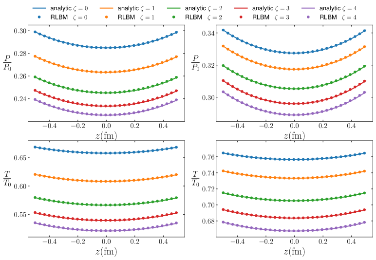
Figure 2: Comparison of numerical results for the Bjorken flow of an ideal gas of particles with different values of the relativistic coldness $\zeta$, computed with respect to the reference temperature $k_{\rm B}T_{0}=300$ MeV. Represented in the figure are the Pressure and Temperature profiles in the $z$ spatial domain, taken at time $t=2$ fm/c, both considering a $d=2$ (left column) and $d=3$ (right column) ideal Equation of State. The numerical results are confronted with the analytic ($\zeta=0$) and semi-analytic ($\zeta\neq 0$) results, and a perfect match is obtained.

We take as initial value for the temperature $T(t_{0},z_{0})=T_{0}=300~{}\rm{MeV}$, that is approximately the value given by both theoretical [28] and lattice QCD  [38] calculations, and is well above the Hagedorn temperature  [32]. Following [39], we set the particle number to $n(t_{0},z_{0})=n_{0}=1.5~{}\rm{fm}^{-d}$.

We select the following values for the relativistic coldness $\zeta=mc^{2}/k_{\rm B}T_{0}$: $\zeta=(0,1,2,3,4)$, that with the value chosen for $T_{0}$ roughly translate to rest masses that fall within the quark mass range [40].

The macroscopic fields $n(t_{0},z)$, $T(t_{0},z)$ are initialized from Eq. 3.1 (or by numerically solving Eq. 26 in the case $\zeta\neq 0$), while the macroscopic velocity $U^{\alpha}(t_{0},z)$ is set according to Eq. 16.

The discrete particle distribution functions $f_{i}$ are initialized at equilibrium

$$f_{i}(t_{0},z)=f^{{\mbox{\tiny eq}}}_{i}\left(n(t_{0},z),T(t_{0},z),U^{\alpha}(t_{0},z)\right)\quad.$$ (33)

We implement boundary conditions along the $z$ axis using the following expression:

$$f_{i}\left(t,z=\pm\left(\frac{L}{2}+dz\right)\right)=f^{{\mbox{\tiny eq}}}_{i}\left(n_{*}(t,z),T_{*}(t,z),U_{*}^{\alpha}(t,z)\right)+\phi_{i}\quad,$$ (34)

where quantities denoted with the subscript “*” are calculated from Eq. 3.1 and Eq. 16, and with $\phi_{i}$ a zero-th order extrapolation of the non-equilibrium part of the distribution calculated from the inner grid points.

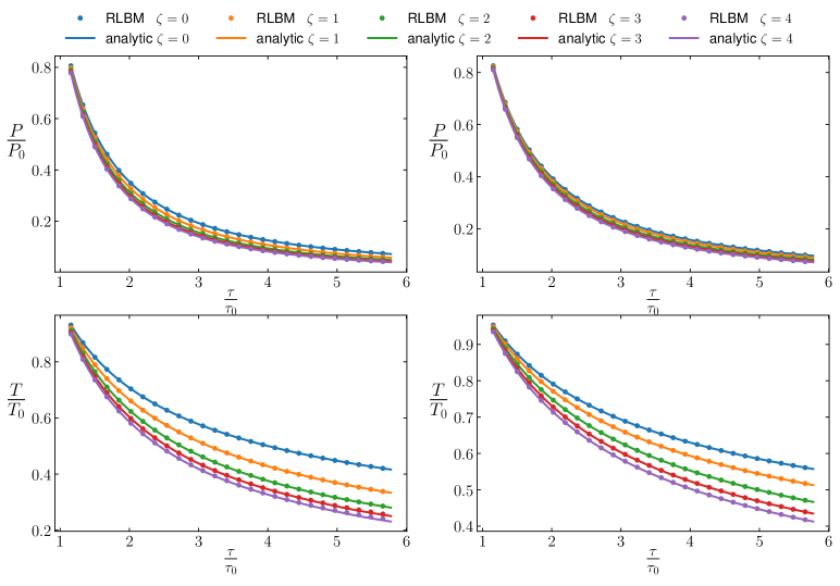
Figure 3: Comparison of numerical results for the Bjorken flow of an ideal gas of particles with different values of the relativistic coldness $\zeta$, computed with respect to the reference temperature $k_{\rm B}T_{0}=300$ MeV. Represented in the figure are the Pressure and Temperature profiles in the $\uptau$ time domain, both considering a $d=2$ (left column) and $d=3$ (right column) ideal Equation of State. The initial value for $\uptau_{0}$ is computed according to 32, where $L=1$ fm and $t_{0}=1$ fm/c. The numerical results are confronted with the analytic ($\zeta=0$) and semi-analytic ($\zeta\neq 0$) results, and a perfect match is obtained.

In Fig. 2 and Fig. 3 we compare numerical results from RLBM simulations against the analytic solutions presented in Sec. 3.

In Fig. 2 we show the profiles for temperature and pressure as a function of the spatial coordinate $z$. The snapshots are taken at $t=2~{}\rm{fm/c}$. The macroscopic profiles are in excellent agreement with the analytic solution.

In the panels on the left hand side we report results in $(2+1)$ dimensions, while on the right we show the results in $(3+1)$ dimensions. Although the flow is mono-dimensional, the number of spatial dimensions enters the definition of the EOS 8. We observe that the evolution of the QGP phase is accelerated in the $(2+1)$-dimensional case, with the gas cooling down at a quicker rate with respect to the $(3+1)$ counterpart.

Moreover, from Fig. 2 it is possible to appreciate that the evolution of fluids consisting of heavier particles leads to lower temperature values and therefore to a quicker cooling of the QGP. This suggests that such cases would lead to phase transitions at an earlier time, in complete consistence with theoretical calculations and experimental observations  [41] and providing a basis for more complex coalescence models  [42].

Finally, in Fig. 3 we give a different representation of Fig. 2, with the macroscopic profiles presented as function of the Milne coordinate $\uptau$. We once again stress that the RLBM used in this work operates in Minkowski coordinates; the results in Fig. 3 have been translated into the Milne spacetime via a simple coordinate transformation thanks to the fact that all the thermodynamic fields are Lorentz scalars.

5 Conclusions

In this work, we have presented analytic and numerical solutions describing a Bjorken flow in a flat space-time coordinate system. This type of benchmark provides a simplified description of the longitudinal expansion of the QGP, mimicking the dynamics observed in relativistic heavy ion collisions taking place in particle colliders such as RHIC and LHC.

We have considered the dynamics of a relativistic fluid for several kinematic parameters, in particular varying the rest mass of the particles, as well as the equation of state. The numerical results show excellent agreement with the analytic solutions.

This work may provide a useful reference for evaluating the accuracy of numerical solvers for relativistic hydrodynamics working in a Minkowski flat space-time. Furthermore, the proposed solver might be useful for further simulations of QGP, that go beyond the longitudinal description and investigate the transversal motion as well. As an example, study of elliptic flows [43] and characterizations of Bjorken attractors [44, 45] might be natural next steps of investigation.

References

- [1] STAR Collaboration, Experimental and theoretical challenges in the search for the quark–gluon plasma: The star collaboration’s critical assessment of the evidence from rhic collisions, Nuclear Physics A 757 (1) (2005) 102–183, first Three Years of Operation of RHIC. doi:10.1016/j.nuclphysa.2005.03.085.
- [2] PHOBOS Collaboration, The phobos perspective on discoveries at rhic, Nuclear Physics A 757 (1) (2005) 28–101, first Three Years of Operation of RHIC. doi:10.1016/j.nuclphysa.2005.03.084.
- [3] PHENIX Collaboration, Formation of dense partonic matter in relativistic nucleus–nucleus collisions at rhic: Experimental evaluation by the phenix collaboration, Nuclear Physics A 757 (1) (2005) 184–283, first Three Years of Operation of RHIC. doi:10.1016/j.nuclphysa.2005.03.086.
- [4] BRAHAMS Collaboration, Quark–gluon plasma and color glass condensate at rhic? the perspective from the brahms experiment, Nuclear Physics A 757 (1) (2005) 1–27, first Three Years of Operation of RHIC. doi:10.1016/j.nuclphysa.2005.02.130.
- [5] R. Pasechnik, M. Šumbera, Phenomenological review on quark–gluon plasma: Concepts vs. observations, Universe 3 (1) (2017). doi:10.3390/universe3010007.
- [6] H. Satz, The transition from hadron matter to quark-gluon plasma, Annual Review of Nuclear and Particle Science 35 (1) (1985) 245–270. doi:10.1146/annurev.ns.35.120185.001333.
- [7] F. Karsch, Lattice results on qcd thermodynamics, Nuclear Physics A 698 (1) (2002) 199–208, 15th Int. Conf. on Ultra-Relativistic Nucleus-Nucleus Collisions (Quark Matter 2001). doi:10.1016/S0375-9474(01)01365-3.
- [8] W. Busza, K. Rajagopal, W. van der Schee, Heavy ion collisions: The big picture and the big questions, Annual Review of Nuclear and Particle Science 68 (1) (2018) 339–376. doi:10.1146/annurev-nucl-101917-020852.
- [9] A. Jaiswal, V. Roy, Relativistic hydrodynamics in heavy-ion collisions: general aspects and recent developments, Advances in High Energy Physics 2016 (2016). doi:10.1155/2016/9623034.
- [10] P. Romatschke, U. Romatschke, Relativistic Fluid Dynamics In and Out of Equilibrium: And Applications to Relativistic Nuclear Collisions, Cambridge Monographs on Mathematical Physics, Cambridge University Press, 2019. doi:10.1017/9781108651998.
- [11] W. Israel, J. M. Stewart, On transient relativistic thermodynamics and kinetic theory. ii, Proceedings of the Royal Society of London A: Mathematical, Physical and Engineering Sciences 365 (1720) (1979) 43–52. doi:10.1098/rspa.1979.0005.
- [12] R. Baier, P. Romatschke, D. T. Son, A. O. Starinets, M. A. Stephanov, Relativistic viscous hydrodynamics, conformal invariance, and holography, Journal of High Energy Physics 2008 (04) (2008) 100–100. doi:10.1088/1126-6708/2008/04/100.
- [13] B. Schenke, S. Jeon, C. Gale, (3+1)d hydrodynamic simulation of relativistic heavy-ion collisions, Phys. Rev. C 82 (2010) 014903. doi:10.1103/PhysRevC.82.014903.
- [14] E. Molnar, H. Niemi, D. Rischke, Numerical tests of causal relativistic dissipative fluid dynamics, The European Physical Journal C 65 (3) (2010) 615–635. doi:10.1016/j.nuclphysa.2009.10.121.
- [15] L. DelZanna, V. Chandra, G. Inghirami, V. Rolando, A. Beraudo, A. DePace, G. Pagliara, A. Drago, F. Becattini, Relativistic viscous hydrodynamics for heavy-ion collisions with echo-qgp, The European Physical Journal C 73 (8) (2013) 2524. doi:10.1140/epjc/s10052-013-2524-5.
- [16] I. Karpenko, P. Huovinen, M. Bleicher, A 3+1 dimensional viscous hydrodynamic code for relativistic heavy ion collisions, Computer Physics Communications 185 (11) (2014) 3016–3027. doi:10.1016/j.cpc.2014.07.010.
- [17] K. Okamoto, Y. Akamatsu, C. Nonaka, A new relativistic hydrodynamics code for high-energy heavy-ion collisions, The European Physical Journal C 76 (10) (2016) 579. doi:10.1140/epjc/s10052-016-4433-x.
- [18] A. Gabbana, D. Simeoni, S. Succi, R. Tripiccione, Relativistic lattice boltzmann methods: Theory and applications, Physics Reports 863 (2020) 1–63, relativistic lattice Boltzmann methods: Theory and applications. doi:10.1016/j.physrep.2020.03.004.
- [19] Z. Xu, C. Greiner, Transport rates and momentum isotropization of gluon matter in ultrarelativistic heavy-ion collisions, Phys. Rev. C 76 (2007) 024911. doi:10.1103/PhysRevC.76.024911.
- [20] S. Plumari, A. Puglisi, F. Scardina, V. Greco, Shear Viscosity of a strongly interacting system: Green-Kubo vs. Chapman-Enskog and Relaxation Time Approximation, Phys. Rev. C C86 (2012) 054902. arXiv:1208.0481, doi:10.1103/PhysRevC.86.054902.
- [21] K. W. Thompson, The special relativistic shock tube, Journal of Fluid Mechanics 171 (1986) 365–375. doi:10.1017/S0022112086001489.
- [22] J. M. Marti, E. Mueller, The analytical solution of the riemann problem in relativistic hydrodynamics, Journal of Fluid Mechanics 258 (1994) 317–333. doi:10.1017/S0022112094003344.
- [23] I. Bouras, E. Molnár, H. Niemi, Z. Xu, A. El, O. Fochler, C. Greiner, D. H. Rischke, Relativistic Shock Waves in Viscous Gluon Matter, Physical Review Letters 103 (2009) 032301. doi:10.1103/PhysRevLett.103.032301.
- [24] I. Bouras, E. Molnár, H. Niemi, Z. Xu, A. El, O. Fochler, C. Greiner, D. Rischke, Development of relativistic shock waves in viscous gluon matter, Nuclear Physics A 830 (2009) 741c–744c. doi:10.1016/j.nuclphysa.2009.10.121.
- [25] I. Bouras, E. Molnár, H. Niemi, Z. Xu, A. El, O. Fochler, C. Greiner, D. H. Rischke, Investigation of shock waves in the relativistic riemann problem: A comparison of viscous fluid dynamics to kinetic theory, Phys. Rev. C 82 (2010) 024910. doi:10.1103/PhysRevC.82.024910.
- [26] I. Bouras, E. Molnár, H. Niemi, Z. Xu, A. El, O. Fochler, F. Lauciello, C. Greiner, D. H. Rischke, Relativistic shock waves and Mach cones in viscous gluon matter, Journal of Physics: Conference Series 230 (2010) 012045. doi:10.1088/1742-6596/230/1/012045.
- [27] A. Gabbana, S. Plumari, G. Galesi, V. Greco, D. Simeoni, S. Succi, R. Tripiccione, Dissipative hydrodynamics of relativistic shock waves in a quark gluon plasma: Comparing and benchmarking alternate numerical methods, Phys. Rev. C 101 (2020) 064904. doi:10.1103/PhysRevC.101.064904.
- [28] J. D. Bjorken, Highly relativistic nucleus-nucleus collisions: The central rapidity region, Phys. Rev. D 27 (1983) 140–151. doi:10.1103/PhysRevD.27.140.
- [29] S. S. Gubser, Symmetry constraints on generalizations of bjorken flow, Phys. Rev. D 82 (2010) 085027. doi:10.1103/PhysRevD.82.085027.
- [30] J. Anderson, H. Witting, A relativistic relaxation-time model for the boltzmann equation, Physica 74 (3) (1974) 466 – 488. doi:10.1016/0031-8914(74)90355-3.
- [31] F. Jüttner, Das maxwellsche gesetz der geschwindigkeitsverteilung in der relativtheorie, Annalen der Physik 339 (5) (1911) 856–882. arXiv:https://onlinelibrary.wiley.com/doi/pdf/10.1002/andp.19113390503, doi:10.1002/andp.19113390503.
- [32] J. Rafelski (Ed.), Melting Hadrons, Boiling Quarks - From Hagedorn Temperature to Ultra-Relativistic Heavy-Ion Collisions at CERN, Springer International Publishing, 2016. doi:10.1007/978-3-319-17545-4.
- [33] U. W. Heinz, Concepts of heavy-ion physics (2004). arXiv:hep-ph/0407360, doi:10.5170/CERN-2006-001.
- [34] T. Krüger, H. Kusumaatmaja, A. Kuzmin, O. Shardt, G. Silva, E. M. Viggen, The Lattice Boltzmann Method - Principles and Practice, 2016. doi:10.1007/978-3-319-44649-3.
- [35] S. Succi, The Lattice Boltzmann Equation: For Complex States of Flowing Matter, OUP Oxford, 2018. doi:10.1093/oso/9780199592357.001.0001.
- [36] N. Kovvali, Theory and applications of Gaussian quadrature methods, Synthesis Lectures on Algorithms and Software in Engineering, Morgan & Claypool, San Rafael, CA, 2010.
- [37] J.-F. Paquet, Probing the space-time evolution of heavy ion collisions with photons and dileptons, Nuclear Physics A 967 (2017) 184–191, the 26th International Conference on Ultra-relativistic Nucleus-Nucleus Collisions: Quark Matter 2017. doi:10.1016/j.nuclphysa.2017.06.003.
- [38] Z. Fodor, S. Katz, Critical point of QCD at finite t and , lattice results for physical quark masses, Journal of High Energy Physics 2004 (04) (2004) 050–050. doi:10.1088/1126-6708/2004/04/050.
- [39] V. E. Ambruş, R. Blaga, High-order quadrature-based lattice boltzmann models for the flow of ultrarelativistic rarefied gases, Phys. Rev. C 98 (2018) 035201. doi:10.1103/PhysRevC.98.035201.
- [40] Particle Data Group, Review of particle physics, Journal of Physics G: Nuclear and Particle Physics 37 (7A) (2010) 075021. doi:10.1088/0954-3899/37/7a/075021.
- [41] M. Waqas, G. X. Peng, F.-H. Liu, Z. Wazir, Effects of coalescence and isospin symmetry on the freezeout of light nuclei and their anti-particles, Scientific Reports 11 (1) (2021) 20252. doi:10.1038/s41598-021-99455-x.
- [42] R. Fries, V. Greco, P. Sorensen, Coalescence models for hadron formation from quark-gluon plasma, Annual Review of Nuclear and Particle Science 58 (1) (2008) 177–205. doi:10.1146/annurev.nucl.58.110707.171134.
-
[43]
R. Snellings, Elliptic
flow: a brief review, New Journal of Physics 13 (5) (2011) 055008.
doi:10.1088/1367-2630/13/5/055008.
URL https://doi.org/10.1088/1367-2630/13/5/055008 -
[44]
J.-P. Blaizot, L. Yan,
Analytical
attractor for bjorken flows, Physics Letters B 820 (2021) 136478.
doi:https://doi.org/10.1016/j.physletb.2021.136478.
URL https://www.sciencedirect.com/science/article/pii/S0370269321004184 - [45] V. E. Ambruş, S. Busuioc, J. A. Fotakis, K. Gallmeister, C. Greiner, Bjorken flow attractors with transverse dynamics, Phys. Rev. D 104 (2021) 094022. doi:10.1103/PhysRevD.104.094022.