Efficient computation of the volume of a polytope in high-dimensions using Piecewise Deterministic Markov Processes

Abstract

Computing the volume of a polytope in high dimensions is computationally challenging but has wide applications. Current state-of-the-art algorithms to compute such volumes rely on efficient sampling of a Gaussian distribution restricted to the polytope, using e.g. Hamiltonian Monte Carlo. We present a new sampling strategy that uses a Piecewise Deterministic Markov Process. Like Hamiltonian Monte Carlo, this new method involves simulating trajectories of a non-reversible process and inherits similar good mixing properties. However, importantly, the process can be simulated more easily due to its piecewise linear trajectories — and this leads to a reduction of the computational cost by a factor of the dimension of the space. Our experiments indicate that our method is numerically robust and is one order of magnitude faster (or better) than existing methods using Hamiltonian Monte Carlo. On a single core processor, we report computational time of a few minutes up to dimension 500.

1 Introduction

1.1 Volume of polytopes

High dimensional integration and sampling is a pervasive challenge in modern science. A subproblem of prime importance consists of computing the volume of a polytope, a bounded convex set of $\mathbb{R}^{d}$ defined as the intersection of a fixed set of half spaces (H-polytope) or the convex hull of a finite set of vertices (V-polytope). This challenge, of estimating the volume of a set, is closely related to problems in Statistics of computing marginal likelihoods [1] or Bayes factors for comparing competing models [2, 3]. It is also related to problems in Physics of estimating partition functions and free energies [4].

Other applications appear across a range of disciplines. For example, in systems biology, the study of genome wide metabolic models based on systems of ODEs requires studying polytopes defined as the intersection between a hyperplane and the null space of a stoichiometry matrix [5, 6]. In robotics, the computation of reachable sets for time-varying linear systems is based upon special polytopes called zonotopes [7]. In finance, the cross sectional score of a portfolio is defined from the intersection between a simplex (representing assets) and hyperplanes or ellipsoids [8]. In artificial intelligence, ReLU networks can be characterized by the conjunction of a set of linear inequalities which define a polytope in the input domain known as the activation condition [9]. In a related vein, the regularization of neural networks using piecewise affine functions involves the evaluation of the volume of polytopes defined by intersections of these hyperplanes [10].

Complexity-wise, computing the volume is #-P hard irrespective of the representation of the polytope (H-polytope or V-polytope)  [11]. Intuitively, any deterministic algorithm using a polynomial number of points and computing the corresponding convex hull omits an exponentially large fraction of the volume. This observation prompted the development of approximation algorithms delivering $(\varepsilon,\delta)$ approximations, that is volume approximations within a factor $1+\varepsilon$ with a probability at least $1-\delta$ [12, 13]. The complexity of such algorithms is measured by the number of calls to an oracle stating whether a point is inside the polytope, or alternatively computing the intersection between a line and the polytope boundary. Remarkably, over the years, the complexity has been lowered from $O^{\star}(d^{23})$ [14] to $O^{\star}(d^{5})$ [15] using a sequence of balls intersecting the convex body, then from $O^{\star}(d^{4})$ [16] to $O^{\star}(d^{3})$ [17] using a sequence of smooth probability densities restricted to the convex body. The reader is referred to [18] for the full history.

Importantly, it should be stressed that the backbone of such algorithms is a telescoping product (Section 2) whose individual terms are the ratio of the integrals (i) of Gaussians on the polytope, or (ii) of the identity function integrated on the intersection between the polytope and a convex body. The former strategy is theoretically faster but the latter puts less burden on the samplers–see next section, since uniform distributions are used.

While the previous works are remarkable from the theoretical standpoint, it is difficult to turn these algorithms into effective implementations. This task is indeed challenging due to possibly huge constants in the complexities and un-realistic worst cases. This state of affairs recently motivated the development of strategies relaxing the theoretical guarantees, based on novel algorithmic and statistical techniques [19, 20, 21, 22]. While these methods are not provably correct in general, their performances in terms of accuracy and running time have proven satisfactory.

1.2 Samplers

The most recent volume computation algorithms mentioned above rely on a procedure that samples a Gaussian distribution restricted to the polytope. The standard way to sample a probability distribution $\pi$ is to build a Markov chain with invariant distribution $\pi$.

For sampling from a Gaussian distribution restricted to a compact region, a number of Markov chains have been proposed, including the Ball Walk sampler [23], the Hit and Run and coordinate Hit and Run samplers [24, 25, 26, 5], and Hamiltonian Monte Carlo [27, 21].

The Ball Walk is a simple Markov chain where the next point is proposed in a ball centered around the current point. If the proposed point is outside of the polytope, or if it rejected by Metropolis-Hasting, the chain stays at the current point.

By comparison, Hit and Run is a rejection free algorithm: a line passing through the current point is chosen at random, and the next point is sampled from the intersection of this line and the inside of the polytope. While this Hit and Run mixes faster than the Ball Walk sampler, it can get stuck in corners [26, 21]. The computational cost of Hit and Run can be reduced by restricting the lines chosen to axis–coordinate Hit and Run.

Hamiltonian Monte Carlo can also be viewed as a rejection free method. It produces trajectories that are based on Hamiltonian dynamics for a physical system whose potential energy is defined by the Gaussian distribution within the polytope, and reflects the trajectory if it hits the boundary of the polytope. This sampler does not get stuck in corners like Hit and Run and has a very good mixing. However, unlike Hit and Run, the computation of the intersection of the trajectories and the boundary requires inverse trigonometric functions, and the computational cost cannot be reduced like Coordinate Hit and Run.

Another sampler is based on the billiard walk [28], which can be seen as a special case of HMC for uniform distributions, and is amenable to a computational complexity reduction similar to the one of coordinate Hit and Run [20]. This sampler can only target uniform distributions and not Gaussians.

Finally, a new class of samplers based on Piecewise Detereministic Markov Processes (PDMPs) has emerged in the computational statistics community [29]. Recall that a PDMP is a deterministic process in-between random jump events, which occur at a certain rate. Hamiltonian Monte Carlo can actually be seen as a PDMP. However, Hamiltonian Monte Carlo relies entirely on the Hamiltonian flow to preserve the target measure, while most of the PDMP samplers developed to date have straight paths. The target measure is then preserved by changing direction at opportune random times. These methods are non reversible, which prevents the diffusive behavior of reversible chains, and have good properties in high dimension [30].

1.3 Contributions

In this work we introduce the use of a PDMP, the Bouncy Particle Sampler [31], to sample from a Gaussian restricted to a polytope within algorithms for calculating the volume of the polytope. Like Hamiltonian Monte Carlo, the Bouncy Particle Sampler has good mixing properties. Moreover, we show how we can re-use many calculations so that it has a much lower computational overhead. The key idea is that the main computation in sampling from a polytope is checking whether and when a trajectory hits the boundary of the polytope. For the Bouncy Particle Sampler, the trajectories are straight lines. We can use properties of how the trajectories change, for example after reflecting off a boundary, to reduce the cost of recalculating when the trajectory will next hit a given face of the boundary of a $d$-dimensional polytope from $O(d)$ to $O(1)$.

We provide detailed experiments up to dimension 500, and a comparison with Hamiltonian Monte Carlo up to dimension 100. These show that our method can be an order of magnitude faster, for the same level of precision, as the current best algorithms using Hamiltonian Monte Carlo.

2 Volume estimation algorithms

Without loss of generality, we consider a polytope $H$ in $d$ dimensions with the origin $0$ strictly inside $H$. We define the polytope $H$ through a $d\times d$ matrix $A$ and a $d$-vector $b$:

$$H=\{x~{}|~{}\forall i,(Ax)_{i}\leq b_{i}\}.$$

We wish to estimate the volume of $H$,

$$Vol(H)=\int_{H}\mbox{d}x.$$

Our approach is based on the algorithm of [19]. Consider a sequence of isotropic Gaussians with marginal variances $\sigma_{0}^{2}<\sigma_{1}^{2}<...<\sigma_{m}^{2}$. Let $f_{i}$ denote the density of the Gaussian with variance $\sigma_{i}$. We discuss the choice of the variances below, but [19] assumes that $\sigma_{m}$ is sufficiently large so that the Gaussian of variance $\sigma_{m}$ is nearly flat on $H$. These assumptions mean that

$$\int_{H}f_{m}(x)dx = \left(\frac{1}{\sqrt{2\pi}\sigma_{m}}\right)^{d}\int_{H}\exp\left\{\frac{-1}{2\sigma_{m}^{2}}\|x\|^{2}\right\}\mbox{d}x$$

$$\approx \left(\frac{1}{\sqrt{2\pi}\sigma_{m}}\right)^{d}Vol(H).$$

Thus the volume of $H$ can be rewritten as:

$$Vol(H) \approx (2\pi\sigma_{m}^{2})^{d/2}\int_{H}f_{m}(x)dx$$

$$= (2\pi\sigma_{m}^{2})^{d/2}\int_{H}f_{0}(x)dx\ \prod_{i=1}^{m}\frac{\int_{H}f_{i}(x)dx}{\int_{H}f_{i-1}(x)dx}$$

We can rewrite each ratio in the product as:

$$\frac{\int_{H}f_{i}(x)dx}{\int_{H}f_{i-1}(x)dx}=\int_{H}\frac{f_{i}(x)}{f_{i-1}(x)}\frac{f_{i-1}(x)}{\int_{H}f_{i-1}(y)dy}dx,$$ (1)

which is just the expectation of $\frac{f_{i}(X)}{f_{i-1}(x)}$ where $X$ is distributed as a Gaussian with variance $\sigma_{i-1}^{2}$ restricted to $H$. Finally, [19] assumes $\sigma_{0}$ is sufficiently small that almost all the mass of the Gaussian with variance $\sigma_{0}^{2}$ lies within in $H$. This means that $\int_{H}f_{0}(x)\mbox{d}x\approx 1$.

This leads to the following approach to estimate $Vol(H)$:

• Choose $m$, the variances $\sigma^{2}_{0}<\cdots<\sigma^{0}_{m}$ and Monte Carlo sizes $N_{1},\ldots,N_{m}$.

• For each $i=1,\ldots,m$, use an MCMC algorithm, or other, to get $N_{i}$ draws $x^{(i)}_{1},\ldots,x^{(i)}_{N_{i}}$ from a Gaussian with variance $\sigma_{i-1}^{2}$ restricted to $H$.

• For each $i=1,\ldots,m$ construct the estimator of (1) as

  $$\hat{I}_{i}=\frac{1}{N_{i}}\sum_{j=1}^{N_{i}}\frac{f_{i}(x^{(i)}_{j})}{f_{i-1}(x^{(i)}_{j})}.$$ (2)

• Estimate $\log\{Vol(H)\}$ as

  $$\frac{d}{2}(2\pi\sigma_{m}^{2})+\sum_{i=1}^{m}\log(\hat{I}_{i}).$$ (3)

In the original algorithm [32], the number of phases, the variances $\sigma_{i}$ and the number of steps per phase were chosen deterministically, leading to a $O^{\star}(d^{3})$ complexity. In the practical implementation [19], a heuristic was added to find a better sequence of Gaussians, reducing the number of steps. In addition, to reduce the number of steps $N_{i}$, a convergence diagnosis based on a heuristic was added. It uses a sliding window of size $W$ (tied to the mixing time of the random walk) to estimate the ratio of Eq. 2. The number of samples $N_{i}$ is therefore not a fixed number, and tuning $W$ is a non trivial issue [21]. Currently the best implementations of this approach [21], uses Hamiltonian Monte Carlo [33] to sample from the restricted Gaussians in step (2).

In this work, we improve this algorithm in three respects.

First, in using the first Gaussian, $\sigma_{0}$ is chosen so that the Gaussian with variance $\sigma_{0}^{2}$ has probability mass of between $c_{min}$ and $c_{max}$ within $H$. Practically, we use $c_{min}=0.1$ and $c_{max}=0.2$. This introduces an additional term to the estimator – we need to add an estimate of the log of the probability mass that $f_{0}$ places with $H$ to (3). To estimate this probability mass, we sample points from the Gaussian and use rejection sampling. The advantage of this adaptation is that it allows us to take a much larger variance, $\sigma_{0}^{2}$, for the initial Gaussian, and thus a smaller value of $m$.

Second, we remove the stopping criterion on the window size used as a proxy for the number of samples $N_{i}$. The size of the sliding windows $W$ has to be tuned, which proved complicated to do. Furthermore, the target precision was not reliably obtained. We use a different strategy where a global given computational budget $N$ is used (outside of the tuning phase of the random walks). For each Gaussian of variance $\sigma_{i}$, we compute $ess_{i}$ the Effective Sample Size (ESS) per iteration of the random walk using the method described in [34, Section 16.4.2]. Then we choose the target number of samples $(N_{i})_{i\leq m}$ such that each ratio has about the same number of independent samples, i.e. $N_{i}\times ess_{i}\approx N_{j}\times ess_{j}$ for all $i$ and $j$, and $\sum_{i=1}^{m}N_{i}=N$.

Third, as explained in the next section, we introduce a novel strategy to sample the Gaussians.

3 Restricted Gaussian sampling using Piecewise Deterministic Markov Processes (PDMP)

3.1 Bouncy Particle Sampler on Unbounded Space

We describe the PDMPs, and proceed with the Bouncy Particle Sampler on an unbounded space.

PDMP.

A PDMP, $z_{t}$, is a continuous time Markov process defined by:

1. a deterministic flow $\phi_{t}(z)$,

2. a jump rate $\lambda(z)$, and

3. a jump kernel $q(\cdot|z)$.

The process $z_{t}$ follows the deterministic flow until a jump event happens. Jumps happen with probability $\lambda(z(t))dt+o(dt)$ in the interval $[t,t+dt]$. If a jump event happens at time $t$, the process $z_{t}$ jumps using the jump kernel $q$:

$$z_{t}\sim q(\cdot\mid z_{t^{-}}),$$

where $z_{t^{-}}=\lim_{s\rightarrow t,s<t}z_{s}$.

Bouncy Particle Sampler.

For a given target density $\pi$ on $\mathbb{R}^{d}$, the state space of the Bouncy Particle Sampler is extended by adding a velocity vector, yielding the state space:

$$E=\mathbb{R}^{d}\times\mathbb{R}^{d}.$$

Thus the state of our PDMP is $z=(x,v)$ and the target density becomes $\mu(x,v)=\pi(x)p_{v}(v)$ where $p_{v}(\cdot)$ is the density of a multivariate normal of mean $0$ and covariance matrix $I_{d}$. The Bouncy Particle Sampler is defined as follow:

1. $\phi_{t}(x,v)=(x+tv,v)$,

2. $\lambda(x,v)=\max(0,-\langle\nabla_{x}(\log\pi)(x),v\rangle)$, and

3. $q(\cdot|z)=\delta_{R(z)}$ with

   $$R(x,v)=\left(x,v-2\frac{\langle v,\nabla_{x}(\log\pi)(x)\rangle}{\|\nabla_{x}(\log\pi)(x)\|^{2}}\nabla_{x}(\log\pi)(x)\right)$$ (4)

Note that the latter formula corresponds to a reflection of vector $v$ with respect to the gradient of the potential. In practice, computing the jump times requires simulating a Poisson process of intensity $\lambda(z_{t})$. This is done by sampling $u$ from an exponential law of rate 1, then solving for $t$ the equation

$$\int_{0}^{t}\lambda(z_{s})ds=u.$$

For a Gaussian target of the form $\pi(x)\propto\exp(-a\|x\|^{2})$, finding the event times amounts to solving:

$$\int_{0}^{t}\max(0,2a(\langle x,v\rangle+s\langle v,v\rangle))ds=u,$$ (5)

which gives a quadratic equation.

3.2 Bouncy Particle Sampler Restricted to a Polytope

The Bouncy Particle Sampler just introduced requires the target density to be continuous and almost everywhere differentiable. Therefore restriction of a Gaussian to a polytope requires adding jumps whenever the process reaches the boundary [35]. We will write $q_{b}(\cdot\mod z)$ the jump kernel at the boundary.

Our target density is of the form

$$\pi(x)\propto\exp(-a\|x\|^{2})1_{H}(x),$$

for some constant $a$ that depends on the variance of the Gaussian, and where $1_{H}$ is the indicator function of $H$. At a point $x$ of the boundary $\partial H$, we write $n(x)$ the outward normal, $\mathcal{V}_{x}^{+}=\{v\in\mathcal{V}|\langle n(x),v\rangle\geq 0\}$ the set of outgoing velocities, $\mathcal{V}_{x}^{-}=\{v\in\mathcal{V}|\langle n(x),v\rangle<0\}$ the set of in-going velocities. Then the process will target the correct distribution if the jump kernel at the boundary $q_{b}$ satisfies the following condition [35]:

$$\int_{\mathcal{V}_{x}^{-}}\langle n(x),u\rangle q_{b}(x,v|u)du=-\langle n(x),v\rangle,$$ (6)

where $x$ is on the boundary, $n(x)$ the outward normal at $x$, and $v\in\mathcal{V}^{+}$ an outgoing velocity. The simplest dynamics that satisfy (6) are to reflect the trajectory off the boundary, so the new velocity becomes $v^{\prime}$ with

$$v^{\prime}=v-2\frac{\langle n,v\rangle}{\|n\|^{2}}n,$$ (7)

with $n$ the normal to the boundary that was hit.

Finally, the Bouncy Particle Sampler is not always ergodic [31]. To ensure ergodicity, we add a refresh event with constant rate $\lambda_{refresh}$ [31]. At refresh events, the velocity is resampled from its marginal invariant distribution, the multivariate normal distribution.

The full algorithm is described in Algorithm 1, and an example trajectory can be found in Figure 1.

  while $t\leq t_{max}$ do

     compute $\tau_{H}$ the intersection time with $H$

     compute $\tau_{evt}$ the next event time by solving (5).

     compute $\tau_{refresh}$ the next refresh event time

     set $\tau=\min(\tau_{H},\tau_{evt},\tau_{refresh})$

     set $x=x+\tau v$

     set $t=t+\tau$

     if $\tau=\tau_{H}$ then

        let $n$ be the normal of the boundary at intersection

        set $v=v-2\frac{\langle n,v\rangle}{\|n\|}n$ (Eq. 7)

     if $\tau=\tau_{evt}$ then

        set $v=R(x,v)$ (Eq. 4)

     if $\tau=\tau_{refresh}$ then

        resample $v$

Algorithm 1 Bouncy Particle Sampler (BPS).

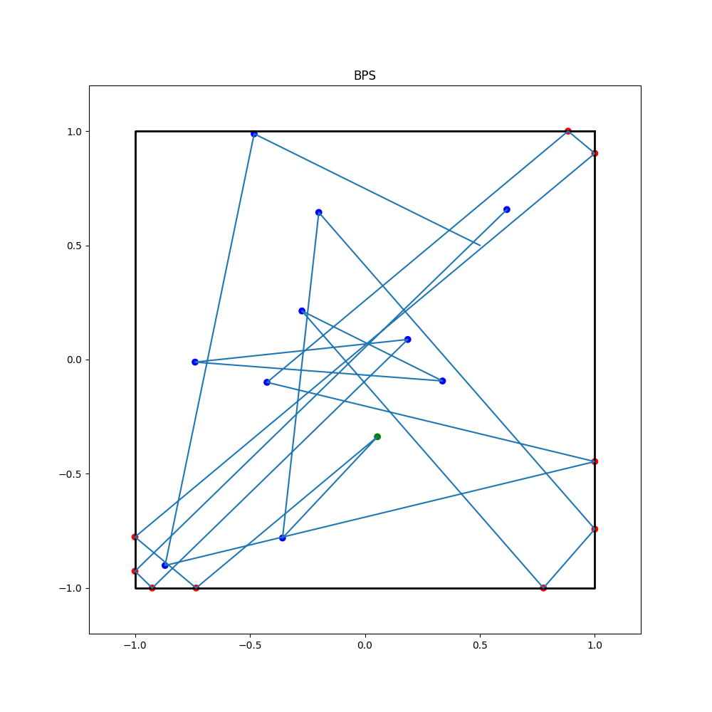
Figure 1: Example BPS trajectory. in the 2d cube $[-1,1]^{2}$, Gaussian of variance $\sigma=1$. Blue: PDMP jump events, Red: reflections on the boundary, Green: refresh events

3.3 Efficient Implementation

An important feature of the Bouncy Particle Sampler is that the velocity is constant between events which leads to deterministic trajectories that are straight-lines. This makes it possible to substantially reduce the computational cost of calculating the times at which the trajectory will hit a boundary. By pre-calculating suitable matrix vector products we can reduce the cost of calculating when the process next hits a boundary from $O(dk)$, where $k$ is the number of hyperplanes that defines $H$, to $O(d)$. This efficient implementation is not possible, for Hamiltonian Monte Carlo samplers due to its non-constant velocity.

Starting from a point $x$ with velocity $v$, the intersection time $\tau_{i}$ for hyperplane $i$ is the solution of $(A(x+tv))_{i}=b_{i}$, in other words $\tau_{i}=\frac{b_{i}-(Ax)_{i}}{(Av)_{i}}$. Finding the intersections for all hyperplanes requires computing the products $Ax$ and $Av$, which leads to a complexity of $dk$. However, in our cases, we keep track of the values of $Ax$ and $Av$ and update them without having to fully recompute the matrix vector product. To update the value of $Ax$ for each event, we use

$$A(x+\tau v)=Ax+\tau Av.$$

Two cases are faced:

Case 1: Reflection on the boundary. First, if the event is a reflection on the boundary with updated velocity $v^{\prime}$, we have

$$Av^{\prime}=Av-2\frac{\langle n,v\rangle}{\|n\|}An.$$

By precomputing $An$ for each hyperplane of the polytope, we can avoid the matrix multiplication.

Case 2: PDMP jump event. The new velocity $v^{\prime}$ is the reflection of $v$ with respect to the gradient of the potential. In the case of Gaussians, the gradient is colinear with $x$. Hence $v^{\prime}=v-2\frac{\langle x,v\rangle}{\|x\|}x$, and we can write

$$Av^{\prime}=Av-2\frac{\langle x,v\rangle}{\|x\|}Ax.$$

Since $Ax$ is known, we can also avoid the matrix-vector product.

Finally, note that for a refresh event, we have no choice but to recompute the matrix-vector product. In practice the proportion of events that are of this type is small.

Remark 1.

In [6], a similar strategy is used for reflection on the boundary, in a setting where there is no PDMP jump event.

3.4 Tuning parameters of the Bouncy Particle Sampler

The Bouncy Particle Sampler has two parameters that requires to be tuned. We describe here the automatic tuning strategy we implemented.

The Bouncy Particle Sampler is currently described as a continuous time process. To extract points from the trajectory $z_{t}$, we add another Poisson rate $\lambda_{out}$. Each time an event happens with respect to this Poisson process, the current point $z_{t}$ is passed to the volume computation algorithm. To tune $\lambda_{out}$, we use the following heuristic: to get a sample independent from the starting point, we require $d$ events (see Cases 1 and 2 above) to happen. Hence, we automatically tune $\lambda_{out}$ at runtime so that there is on average $d$ events between points passed to the volume algorithm.

Furthermore, as noted before, we have a refresh rate $\lambda_{refresh}$, whose tuning is important for the mixing time. To tune this parameter, we use an optimization procedure described in more details in Section 5.2.

4 Implementation and multiprecision

4.1 Code overview

Our code is written in C++, using the number types discussed below. ESS calculations were carried out using the Autoppl library https://github.com/JamesYang007/autoppl.

4.2 Multiprecision

Trajectories escaping the polytope. As noted in [21], Hamiltonian Monte Carlo trajectories can escape the polytope due to numerical issues – a phenomenon becoming prevalent in high dimension. The solution introduced in [21] is to recompute a trajectory leaving the convex by using interval arithmetic with increased precision.

Since the trajectory escaping the polytope can lead to a completely wrong estimate at best, and a crash of the program at worse, a similar strategy is used in this work. Assuming the $T_{k}$ are the output times of the trajectories that are passed to the volume algorithm (i.e. the sequence used by the volume algorithm is $(x_{T_{k}})_{k\in\mathbb{N}}$ ), the strategy is as follow:

1. at time $T_{i}$, save the state of the Bouncy Particle Sampler: $x_{T_{i}}$ and $v_{T_{i}}$, but also the state of the random generator;

2. compute the trajectory using double precision until time $T_{i+1}$;

3. if $x_{T_{i+1}}$ is in the polytope, nothing needs to be done;

4. else:

   1. roll back the state of the Bouncy Particle Sampler to time $T_{i}$.

   2. increase the precision of real numbers used in the previous step.

   3. compute the trajectory until time $T_{i+1}$.

   4. repeat until $x_{T_{i+1}}$ is in the polytope.

It should also be noticed that precision cannot be increased indefinitely. As a fallback, if the required precision reaches a certain threshold, we go back to time $T_{i}$ and sample a new velocity. In the Experiments below, we report on these outcomes using two statistics:

• $\#M$: the number of times the else above is entered.

• $\#R$: the number of times the precision limit is reached.

Number types. To handle precision refinements, we use the number type boost::multiprecision::mpfr_float.

Numerical values for volumes. Multiprecision is also required to compute the volume, in two guises. On the one hand, the exact volume of the polytopes used in our tests cannot be represented using double precision, when increasing the dimension. On the other hand, high precision floating points must be used when computing the exponential of the sum of the log of the ratios $\sum_{i=1}^{m}\log(\hat{I}_{i})$. To handle these difficulties, we use the number type
boost::multiprecision::cpp_dec_float, which makes it possible to specify the number of decimal digits used.

5 Experiments

5.1 Setup and statistics of interest

Polytopes.

We study our algorithm for three polytopes where the exact volume is known:

• The cube, $-1\leq x_{i}\leq 1$, for $i=1,\ldots,d$.

• The standard simplex ($\Delta_{\text{std}}$), $\sum x_{i}\leq 1$, $x_{i}\geq 0$.

• The isotropic simplex ($\Delta_{\text{iso}}$), a simplex which is also a regular polytope.

Targeting a given error.

Assessing the complexity of our algorithm as a function of the dimension–for a given polytope, requires finding the number of samples for which a target error on the volume estimate is obtained. To this end, consider a minibatch of repeats (24 in our case to exploit brute force parallelism on our computer), each using $N$ samples. We run a binary search on $N$ to obtain the smallest value for which the median error of the minibatch lies in the interval $4\%\pm 1\%$. (Nb: to speed up calculations, the binary search is also exited if the number of samples between two consecutive runs varies less than 5%.)

In this experiment, the dimensions $d=50,70,100,140,175,250$ are used for each polytope. For a given statistic of interest (the median running time or the final number of samples $N$), we then perform a linear regression in log log scale, to assess the polynomial scaling of the statistic.

The output of each computation contains

• the final estimation of the volume,

• the run-time (in seconds), and

• the number of times the precision had to be increased to stay in the polytope.

Using a fixed number of samples.

To compare PDMP against state-of-the-art volume algorithms based on Hamiltonian Monte Carlo [21], we resort to experiments at a fixed number of samples. The volume computation is launched for dimension $d=100,500$, using sample sizes $N=10^{5},10^{6},10^{7}$ – the latter for $d=500$ only.

Computer used.

Calculations were run on a desktop DELL Precision 7920 Tower (Intel Xeon Silver 4214 CPU at 2.20GHz, 64 Gb of RAM), under Linux Fedora core 34.

5.2 Tuning

Based on the results in [36], heuristically, a small refresh rate will lead to better mixing for individual coordinates of the samples, whereas a higher refresh rate will mean better mixing for functionals such as the norm of the position. In our case, bouncing on the boundary of the polytope can play a similar role to refreshing the velocity. Hence we expect the optimal refresh rate to depend on the variance of the sampled restricted Gaussian.

Thus we compute the ESS for the projection on each coordinate, and take the minimum, which we call $ess_{min}$. Further we compute $ess_{norm}$, the ESS associated to the norm of our samples. If $ess_{min}<ess_{norm}$, we decrease the refresh rate $\lambda_{refresh}$, and if $ess_{min}>ess_{norm}$, we increase the refresh rate.

However, refreshing the velocity is expensive, since it requires recomputing the matrix-vector product $Av$, with a cost of $O(d^{2})$ instead of $O(d)$ for other events. Thus the new refresh rate is only accepted if it leads to a higher ESS per second, with the overall ESS being $min(ess_{min},ess_{norm})$. If not, the tuning is stopped (Fig. 2).

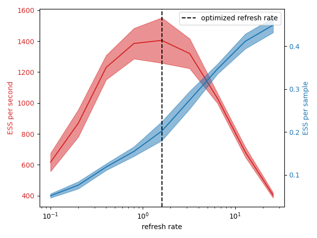
Figure 2: ESS optimization of the resfresh rate $\lambda_{refresh}$. Model: cube of dimension $100$. We show in red the ESS per second and in blue the ESS per sample around the optimized value for $\lambda_{refresh}$. The ESS is computed with $10000$ samples. The solid red and blue lines are the avarage of the ESS and the envelop represents the standard deviation of the ESS.

The number of consecutive samples used to evaluate the ESS results from a tradeof between the quality of the tuning, which increases with number of samples, and the time spent tuning the walk with In our experiments, the number of consecutive samples is restricted by runs in dimension 500, which leads us to use 100 consecutive samples to evaluate the ESS. is advised.

5.3 Results

PDMP: complexity.

The experiments at prescribed error rate show a clear polynomial time complexity (Fig. 3), with a scaling around $O(d^{3.5})$ for the three test polytopes (Table 1). In particular, we can see that the time complexity is close to the number of samples times $d^{2}$. This is consistent with intuition, since each sample requires on average $O(d)$ events, and each event (except for refresh events) requires $O(d)$ computations.

	Time		Num. samples
model	slope	$R^{2}$	slope	$R^{2}$
cube	3.77	0.96	1.94	0.88
$\Delta_{\text{iso}}$	3.52	1.00	1.72	0.99
$\Delta_{\text{std}}$	3.18	0.99	1.37	0.96

Table 1: Linear regression in log log scale for the three polytopes. First variable regressed: running time (seconds); second variable: number of samples $N$ used to obtain a prescribed error estimate on the volume.

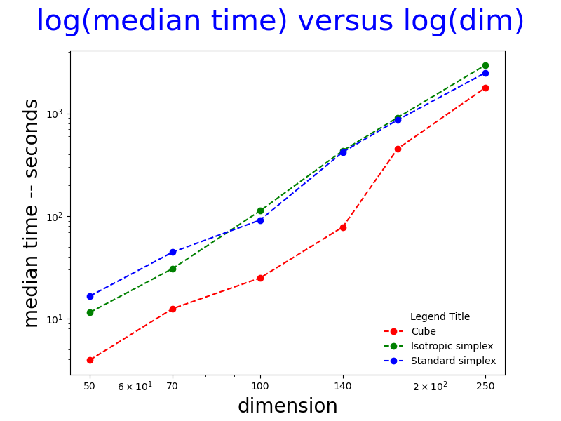
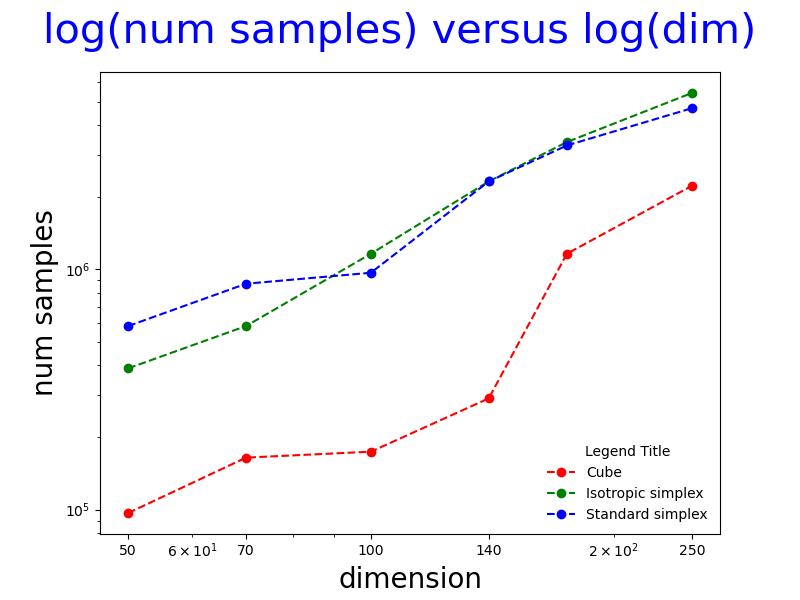
Figure 3: Complexity of PDMP studied using the smallest number of samples achieving a target error estimate for each polytope. Dimensions used: $d=50,70,100,140,175,250$. Plots are in log log scale. (Top) Time as a function of dimension (Bottom) Number of samples as a function of dimension. See also Table 1.

PDMP versus HMC: complexity.

Hamiltonian Monte Carlo based methods require the specification of a so-called window size used to determine convergence of the ratio of (1) [21]. In the sequel, we use two window sizes:

• Low profile comparison: the window size $W=250$ is used to compare Hamiltonian Monte Carlo against PDMP with $10^{5}$ samples – short-hand: HMC1;

• High profile comparison: the window size $W=250+d\sqrt{d}$ is used to compare Hamiltonian Monte Carlo against PDMP with $10^{6}$ samples – short-hand: HMC2.

Two facts stand out (Tables S3 and S4). On the one hand, for the three polytopes, the two algorithms compared yield equivalent error estimates. On the other hand, PDMP yields a speedup between one and two orders of magnitude over HMC. To be precise, in dimension $d=100$ e.g.: between $\sim$ 56 and 135 for the low profile comparison, and between $\sim$ 14 and 44 for the high profile comparison. This comparison shows the superiority of linear trajectories over curved ones in HMC.

As a final analysis, we challenge PDMP with calculations up to dimension $d=500$, using a fixed number of samples (Tables S8.2 and S8.2). Obtaining a relative error below 10% now requires using a number of samples $N$ one order of magnitude larger. Still, with a running time of the order of hours, such large dimensions remain tractable.

PDMP versus HMC: numerics.

Another important issue is that of numerical robustness faced by geometric algorithms in general [37]. Along with the volumes, we monitor the number of multi-precision refinements – Table S8.1. In sharp contrast with the method based on Hamiltonian Monte Carlo [21], such refinements are not triggered by the PDMP sampler – the statistic #M is null and therefore so is #R. We conjecture that multiprecision is required with HMC due to intersections between curved trajectories and the polytope boundary, requiring the (numerically challenging) computation of an $\arctan$.

Cooling schedules: using Gaussians versus balls.

As mentioned in the Introduction, an alternative algorithm uses balls intersected with the polytope instead of Gaussians restricted to the polytope [20]. Since this algorithm only requires uniform sampling, the simpler billiard walk sampler can be used [20]. It should be noted than our sampling strategies are essentially the same than the one provided in [20], the main difference being that our random walk handle Gaussians while still having a low computational complexity.

Ball cooling essentially amounts to changing the functions $f_{i}$ in Eq. (2) from Gaussian densities to indicator functions of balls. In that case, the ratio found in Eq. (2) is exactly $0$ or $1$. In principle, this should lead to a higher variance of $\hat{I}_{i}$ of Eq. (2) than for Gaussians, which would be less efficient. This is consistent with known theoretical results [15, 17] which seems to indeed indicate a greater efficiency of the Gaussian cooling compared to balls.

Interestingly, the implementation provided in the preprint [20] yields better results, which contradicts theory [15, 17]. This calls for further analysis in two directions. The first is the analysis of the cooling schedule based on a sequence of balls [20] versus a sequence of Gaussians [19]. The second one is the tuning of the random walk generating samples (in our case: refresh rate $\lambda_{refresh}$, output rate $\lambda_{output}$).

We believe that two things might be happening. First, the tuning strategy used for balls might outperform ours, which is expensive since it relies on calculating the ESS. Second, we rely on the sequence of Gaussians provided by [19], while a new one, possibly more optimal for balls, is used in [20].

6 Code availability

Visit the github repo https://github.com/augustin-chevallier/PolytopeVolume.

7 Conclusion

Recent developments for polytope volume calculation algorithms have exploited two strategies, namely using a sequence of Gaussians or a sequence of balls intersecting the polytope. Our work presents improvements for the former, yielding a substantial speedup (more than one order of magnitude on running times) over state-of-the-art HMC based methods. On the other hand, recent work in the latter vein has resulted in faster and more accurate results [20], an unexpected observation given the theoretical bounds known to date for both classes of methods. An interesting avenue for future work will therefore consist of hybridising both approaches.

For convex bodies with piecewise $C^{1}$ boundaries, our algorithm could also be applied. While the improvement to the oracle complexity might not apply, the intersection of linear trajectories with the boundary would improve on HMC.

On the practical aspect, there are a few improvements that could be made in future work. The most obvious one would be to re-use the points sampled at previous phases using importance sampling. The second would be to introduce a way of refreshing velocities that do not require recomputing the matrix-vector product.

Polytope volume calculations algorithms first underwent major improvements in the theoretical realm (with bounds on the mixing times but algorithms lacking efficiency in practice), and more recently in the practical realm (with efficient algorithms lacking theoretical bounds). Combining both is clearly an outstanding challenge ahead.

Acknowledgments. We thank Sylvain Pion for stimulating discussions on numerical issues.

This work has been partially supported by the French government, through the 3IA Côte d’Azur Investments in the Future project managed by the National Research Agency (ANR) with the reference number ANR-19-P3IA-0002, and EPSRC grants EP/R034710/1 and EP/RO18561/1.

8 Supporting Information

8.1 Comparisons at a fixed error rate

• Table S8.1 and Table S8.1 present the full results corresponding to the protocol Targeting a given error from Section 5.

N	Algo.	model	$d$	$\varepsilon$	$Vol$	$\min\tilde{V}$	$\max\tilde{V}$	$med(\tilde{V})$	$stdev(\tilde{Vol})$	$med(\text{err}_{r})$	$stdev(\text{err}_{r})$
24	PDMP-N9.7e+04	cube	50	NA	1.126e+15	1.04e+15	1.292e+15	1.129e+15	5.653e+13	3.089E-02	3.410E-02
24	PDMP-N1.6e+05	cube	70	NA	1.181e+21	1.106e+21	1.296e+21	1.155e+21	5.099e+19	3.563E-02	2.459E-02
24	PDMP-N1.7e+05	cube	100	NA	1.268e+30	1.125e+30	1.423e+30	1.254e+30	6.966e+28	3.075E-02	3.619E-02
24	PDMP-N2.9e+05	cube	140	NA	1.394e+42	1.245e+42	1.553e+42	1.386e+42	8.808e+40	5.590E-02	2.983E-02
24	PDMP-N1.2e+06	cube	175	NA	4.789e+52	4.469e+52	5.235e+52	4.825e+52	2.368e+51	4.301E-02	2.697E-02
24	PDMP-N2.2e+06	cube	250	NA	1.809e+75	1.662e+75	1.968e+75	1.81e+75	7.275e+73	2.300E-02	2.593E-02
24	PDMP-N3.9e+05	$\Delta_{\text{iso}}$	50	NA	3.421e+21	3.173e+21	3.65e+21	3.419e+21	1.127e+20	2.462E-02	1.968E-02
24	PDMP-N5.8e+05	$\Delta_{\text{iso}}$	70	NA	1.658e+30	1.529e+30	1.888e+30	1.64e+30	7.302e+28	3.066E-02	2.955E-02
24	PDMP-N1.2e+06	$\Delta_{\text{iso}}$	100	NA	1.771e+43	1.648e+43	1.847e+43	1.783e+43	4.733e+41	1.739E-02	1.675E-02
24	PDMP-N2.3e+06	$\Delta_{\text{iso}}$	140	NA	4.167e+60	3.855e+60	4.441e+60	4.223e+60	1.73e+59	3.069E-02	2.139E-02
24	PDMP-N3.4e+06	$\Delta_{\text{iso}}$	175	NA	6.607e+75	5.94e+75	6.928e+75	6.66e+75	2.726e+74	2.896E-02	2.755E-02
23	PDMP-N5.4e+06	$\Delta_{\text{iso}}$	250	NA	2.466e+108	2.22e+108	2.762e+108	2.466e+108	1.223e+107	2.916E-02	3.131E-02
24	PDMP-N5.8e+05	$\Delta_{\text{std}}$	50	NA	3.288e-65	3.136e-65	3.525e-65	3.254e-65	1.144e-66	2.917E-02	1.702E-02
24	PDMP-N8.7e+05	$\Delta_{\text{std}}$	70	NA	8.348e-101	7.864e-101	9.148e-101	8.437e-101	3.563e-102	2.716E-02	2.651E-02
24	PDMP-N9.7e+05	$\Delta_{\text{std}}$	100	NA	1.072e-158	9.614e-159	1.191e-158	1.084e-158	5.896e-160	2.851E-02	3.276E-02
24	PDMP-N2.3e+06	$\Delta_{\text{std}}$	140	NA	7.428e-242	6.621e-242	7.962e-242	7.264e-242	3.31e-243	3.717E-02	3.101E-02
24	PDMP-N3.3e+06	$\Delta_{\text{std}}$	175	NA	8.893e-319	8.029e-319	9.465e-319	8.672e-319	4.164e-320	4.609E-02	2.545E-02
24	PDMP-N4.7e+06	$\Delta_{\text{std}}$	250	NA	3.093e-493	2.751e-493	3.611e-493	3.062e-493	2.114e-494	5.489E-02	3.935E-02

Table S  1: Statistics on volumes and their estimates. See text for details.

N	Algo.	model	$d$	$\varepsilon$	med($\#O/\#S$)	stdev($\#O/\#S$)	med($\#M$)	med($\#R$)	med(time)	stdev(time)
24	PDMP-N9.7e+04	cube	50	NA	5.502E+01	1.120E+00	0	0	3.980E+00	1.349E-01
24	PDMP-N1.6e+05	cube	70	NA	7.661E+01	1.683E+00	0	0	1.257E+01	3.556E-01
24	PDMP-N1.7e+05	cube	100	NA	1.075E+02	2.906E+00	0	0	2.497E+01	8.915E-01
24	PDMP-N2.9e+05	cube	140	NA	1.525E+02	4.738E+00	0	0	7.820E+01	2.079E+00
24	PDMP-N1.2e+06	cube	175	NA	1.870E+02	6.107E+00	0	0	4.523E+02	9.362E+00
24	PDMP-N2.2e+06	cube	250	NA	2.655E+02	6.158E+00	0	0	1.774E+03	4.370E+01
24	PDMP-N3.9e+05	$\Delta_{\text{iso}}$	50	NA	5.325E+01	4.078E-01	0	0	1.153E+01	1.755E-01
24	PDMP-N5.8e+05	$\Delta_{\text{iso}}$	70	NA	7.398E+01	7.903E-01	0	0	3.078E+01	7.514E-01
24	PDMP-N1.2e+06	$\Delta_{\text{iso}}$	100	NA	1.049E+02	1.349E+00	0	0	1.126E+02	1.651E+00
24	PDMP-N2.3e+06	$\Delta_{\text{iso}}$	140	NA	1.473E+02	2.441E+00	0	0	4.331E+02	5.064E+00
24	PDMP-N3.4e+06	$\Delta_{\text{iso}}$	175	NA	1.815E+02	2.603E+00	0	0	9.097E+02	1.406E+01
23	PDMP-N5.4e+06	$\Delta_{\text{iso}}$	250	NA	2.594E+02	2.725E+00	0	0	2.944E+03	5.608E+01
24	PDMP-N5.8e+05	$\Delta_{\text{std}}$	50	NA	5.287E+01	4.716E-01	0	0	1.663E+01	2.769E-01
24	PDMP-N8.7e+05	$\Delta_{\text{std}}$	70	NA	7.310E+01	5.935E-01	0	0	4.453E+01	8.768E-01
24	PDMP-N9.7e+05	$\Delta_{\text{std}}$	100	NA	1.039E+02	8.778E-01	0	0	9.153E+01	1.698E+00
24	PDMP-N2.3e+06	$\Delta_{\text{std}}$	140	NA	1.444E+02	1.641E+00	0	0	4.197E+02	4.341E+00
24	PDMP-N3.3e+06	$\Delta_{\text{std}}$	175	NA	1.799E+02	1.238E+00	0	0	8.625E+02	1.202E+01
24	PDMP-N4.7e+06	$\Delta_{\text{std}}$	250	NA	2.560E+02	1.543E+00	0	0	2.481E+03	2.766E+01

Table S  2: Misc statistics. The columns read as follows: $\varepsilon$: precision target (NA for PDMP) $\#S$: num samples. $\#O/\#S$: num calls to the oracle per sample $\#M$: number of multi-precision refinements. $\#R$: number of calls to resample.

8.2 Comparisons at a fixed number of samples

• Tables S3 and S4 present a comparison between HMC and PDMP, in dimensions $d=50$ and $d=100$.

• Table S8.2 and Table S8.2 present the full results corresponding to the protocol Using a fixed number of samples from Section 5.

Algorithm	Model	$med(\text{err}_{r})$	$med(time)$
HMC1	cube	3.563E-02	1.076E+02
HMC2	cube	2.363E-02	1.452E+02
PDMP-$10^{5}$	cube	2.731E-02	4.025E+00
PDMP-$10^{6}$	cube	2.248E-02	3.583E+01
HMC1	$\Delta_{\text{iso}}$	5.191E-02	1.164E+02
HMC2	$\Delta_{\text{iso}}$	3.181E-02	1.798E+02
PDMP-$10^{5}$	$\Delta_{\text{iso}}$	4.751E-02	3.712E+00
PDMP-$10^{6}$	$\Delta_{\text{iso}}$	2.394E-02	2.877E+01
HMC1	$\Delta_{\text{std}}$	6.691E-02	2.302E+02
HMC2	$\Delta_{\text{std}}$	5.715E-02	3.655E+02
PDMP-$10^{5}$	$\Delta_{\text{std}}$	4.624E-02	3.702E+00
PDMP-$10^{6}$	$\Delta_{\text{std}}$	2.760E-02	2.907E+01

Table S  3: Comparison PDMP versus HMC in dimension $d=50$. Results are for cube, isostropic-simplex ($\Delta_{\text{iso}}$) and standard-simplex ($\Delta_{\text{std}}$). HMC- Hamiltonian Monte Carlo based methods from [21]; PDMP – this work with sample sizes $N=10^{5}$ and $N=10^{6}$. HMC1: $W=250$; HMC2: $W=250+d^{1.5}$

Algorithm	Model	$med(\text{err}_{r})$	$med(time)$
HMC1	cube	4.221E-02	9.122E+02
HMC2	cube	2.274E-02	1.765E+03
PDMP-$10^{5}$	cube	4.421E-02	1.506E+01
PDMP-$10^{6}$	cube	2.104E-02	1.261E+02
HMC1	$\Delta_{\text{iso}}$	5.782E-02	7.285E+02
HMC2	$\Delta_{\text{iso}}$	3.469E-02	1.671E+03
PDMP-$10^{5}$	$\Delta_{\text{iso}}$	6.347E-02	1.368E+01
PDMP-$10^{6}$	$\Delta_{\text{iso}}$	3.324E-02	9.637E+01
HMC1	$\Delta_{\text{std}}$	8.130E-02	1.755E+03
HMC2	$\Delta_{\text{std}}$	4.200E-02	4.424E+03
PDMP-$10^{5}$	$\Delta_{\text{std}}$	1.054E-01	1.350E+01
PDMP-$10^{6}$	$\Delta_{\text{std}}$	2.856E-02	9.465E+01

Table S  4: Comparison PDMP versus HMC in dimension $d=100$. Results are for cube, isostropic-simplex ($\Delta_{\text{iso}}$) and standard-simplex ($\Delta_{\text{std}}$). HMC- Hamiltonian Monte Carlo based methods from [21]; PDMP – this work with sample sizes $N=10^{5}$ and $N=10^{6}$. HMC1: $W=250$; HMC2: $W=250+d^{1.5}$

N	Algo.	model	$d$	$\varepsilon$	$Vol$	$\min\tilde{V}$	$\max\tilde{V}$	$med(\tilde{V})$	$stdev(\tilde{Vol})$	$med(\text{err}_{r})$	$stdev(\text{err}_{r})$
48	PDMP-N10**5	cube	100	NA	1.268e+30	1.08e+30	1.505e+30	1.253e+30	8.121e+28	4.421E-02	4.029E-02
48	PDMP-N10**6	cube	100	NA	1.268e+30	1.189e+30	1.332e+30	1.259e+30	3.594e+28	2.104E-02	1.544E-02
48	PDMP-N10**5	cube	500	NA	3.273e+150	1.193e+150	6.295e+150	2.656e+150	1.173e+150	2.955E-01	2.033E-01
48	PDMP-N10**6	cube	500	NA	3.273e+150	2.289e+150	4.084e+150	3.197e+150	4.064e+149	9.948E-02	6.933E-02
24	PDMP-N10**7	cube	500	NA	3.273e+150	2.868e+150	3.593e+150	3.25e+150	1.666e+149	3.969E-02	3.274E-02
48	PDMP-N10**5	$\Delta_{\text{iso}}$	100	NA	1.771e+43	1.31e+43	2.145e+43	1.697e+43	1.819e+42	6.347E-02	6.675E-02
48	PDMP-N10**6	$\Delta_{\text{iso}}$	100	NA	1.771e+43	1.586e+43	1.948e+43	1.754e+43	8.567e+41	3.324E-02	2.850E-02
48	PDMP-N10**5	$\Delta_{\text{iso}}$	500	NA	9.235e+216	1.311e+216	2.292e+217	5.133e+216	4.806e+216	5.364E-01	3.031E-01
48	PDMP-N10**6	$\Delta_{\text{iso}}$	500	NA	9.235e+216	4.967e+216	1.38e+217	9.04e+216	1.938e+216	1.410E-01	1.284E-01
24	PDMP-N10**7	$\Delta_{\text{iso}}$	500	NA	9.235e+216	7.16e+216	1.123e+217	9.113e+216	9.188e+215	4.407E-02	6.582E-02
48	PDMP-N10**5	$\Delta_{\text{std}}$	100	NA	1.072e-158	7.873e-159	1.537e-158	1.081e-158	1.752e-159	1.054E-01	9.916E-02
48	PDMP-N10**6	$\Delta_{\text{std}}$	100	NA	1.072e-158	9.567e-159	1.177e-158	1.085e-158	5.308e-160	2.856E-02	2.991E-02
48	PDMP-N10**5	$\Delta_{\text{std}}$	500	NA	8.196e-1135	1.431e-1135	2.249e-1134	5.193e-1135	4.255e-1135	4.676E-01	3.004E-01
48	PDMP-N10**6	$\Delta_{\text{std}}$	500	NA	8.196e-1135	4.838e-1135	1.546e-1134	7.885e-1135	1.859e-1135	1.504E-01	1.487E-01
24	PDMP-N10**7	$\Delta_{\text{std}}$	500	NA	8.196e-1135	7.02e-1135	1.037e-1134	8.099e-1135	7.98e-1136	7.312E-02	6.213E-02

Table S  5: Statistics on volumes and their estimates. See text for details.

N	Algo.	model	$d$	$\varepsilon$	med($\#O/\#S$)	stdev($\#O/\#S$)	med($\#M$)	med($\#R$)	med(time)	stdev(time)
48	PDMP-N10**5	cube	100	NA	1.084E+02	3.456E+00	0	0	1.506E+01	4.787E-01
48	PDMP-N10**6	cube	100	NA	1.094E+02	3.739E+00	0	0	1.261E+02	3.464E+00
48	PDMP-N10**5	cube	500	NA	5.187E+02	5.499E+00	0	0	1.127E+03	6.796E+01
48	PDMP-N10**6	cube	500	NA	5.155E+02	4.751E+00	0	0	6.595E+03	6.420E+02
24	PDMP-N10**7	cube	500	NA	5.123E+02	5.283E+00	0	0	5.729E+04	1.107E+04
48	PDMP-N10**5	$\Delta_{\text{iso}}$	100	NA	1.070E+02	1.309E+00	0	0	1.368E+01	3.791E-01
48	PDMP-N10**6	$\Delta_{\text{iso}}$	100	NA	1.047E+02	1.054E+00	0	0	9.637E+01	1.424E+00
48	PDMP-N10**5	$\Delta_{\text{iso}}$	500	NA	5.240E+02	3.540E+00	0	0	7.503E+02	4.174E+01
48	PDMP-N10**6	$\Delta_{\text{iso}}$	500	NA	5.114E+02	2.122E+00	0	0	3.112E+03	2.659E+02
24	PDMP-N10**7	$\Delta_{\text{iso}}$	500	NA	5.092E+02	2.132E+00	0	0	2.328E+04	2.978E+03
48	PDMP-N10**5	$\Delta_{\text{std}}$	100	NA	1.061E+02	1.022E+00	0	0	1.350E+01	2.935E-01
48	PDMP-N10**6	$\Delta_{\text{std}}$	100	NA	1.037E+02	6.735E-01	0	0	9.465E+01	9.332E-01
48	PDMP-N10**5	$\Delta_{\text{std}}$	500	NA	5.179E+02	3.678E+00	0	0	7.727E+02	6.141E+01
48	PDMP-N10**6	$\Delta_{\text{std}}$	500	NA	5.053E+02	2.175E+00	0	0	3.175E+03	1.058E+02
24	PDMP-N10**7	$\Delta_{\text{std}}$	500	NA	5.050E+02	1.624E+00	0	0	2.744E+04	3.650E+03

Table S  6: Misc statistics. The columns read as follows: $\varepsilon$: precision target (NA for PDMP) $\#S$: num samples. $\#O/\#S$: num calls to the oracle per sample $\#M$: number of multi-precision refinements. $\#R$: number of calls to resample.

References

- [1] Edwin Fong and Chris C Holmes. On the marginal likelihood and cross-validation. Biometrika, 107(2):489–496, 2020.
- [2] Andrew Gelman and Xiao-Li Meng. Simulating normalizing constants: From importance sampling to bridge sampling to path sampling. Statistical Science, 13:163–185, 1998.
- [3] Nial Friel and Jason Wyse. Estimating the evidence–a review. Statistica Neerlandica, 66(3):288–308, 2012.
- [4] Clara D Christ, Alan E Mark, and Wilfred F Van Gunsteren. Basic ingredients of free energy calculations: a review. Journal of Computational Chemistry, 31(8):1569–1582, 2010.
- [5] H. Haraldsdóttir, B. Cousins, I. Thiele, R. Fleming, and S. Vempala. CHRR: coordinate hit-and-run with rounding for uniform sampling of constraint-based models. Bioinformatics, 33(11):1741–1743, 2017.
- [6] A. Chalkis, V. Fisikopoulos, E. Tsigaridas, and H. Zafeiropoulos. Geometric algorithms for sampling the flux space of metabolic networks. In E. Colin de Verdiere and K. Buchin, editors, 37th International Symposium on Computational Geometry (SoCG 2021), 2021.
- [7] M. Althoff, C. Le Guernic, and B.H. Krogh. Reachable set computation for uncertain time-varying linear systems. In Proceedings of the 14th International Conference on Hybrid Systems: Computation and Control, pages 93–102, 2011.
- [8] L. Calès, A. Chalkis, I. Emiris, and V. Fisikopoulos. Practical volume computation of structured convex bodies, and an application to modeling portfolio dependencies and financial crises. arXiv:1803.05861, 2018.
- [9] C. Păsăreanu, H. Converse, A. Filieri, D., and Gopinath. On the probabilistic analysis of neural networks. In Proceedings of the IEEE/ACM 15th International Symposium on Software Engineering for Adaptive and Self-Managing Systems, pages 5–8, 2020.
- [10] H. Robinson. Approximate piecewise affine decomposition of neural networks. IFAC-PapersOnLine, 54(7):541–546, 2021.
- [11] M. Dyer and A. Frieze. On the complexity of computing the volume of a polyhedron. SIAM Journal on Computing, 17(5):967–974, 1988.
- [12] I. Bárány and Z. Füredi. Computing the volume is difficult. Discrete and Computational Geometry, 2(4):319–326, 1987.
- [13] S. Levy. Flavors of Geometry. Cambridge University Press, 1997.
- [14] M. Dyer, A. Frieze, and R. Kannan. A random polynomial-time algorithm for approximating the volume of convex bodies. Journal of the ACM (JACM), 38(1):1–17, 1991.
- [15] R. Kannan, L. Lovász, and M. Simonovits. Random walks and an ) volume algorithm for convex bodies. Random Structures & Algorithms, 11(1):1–50, 1997.
- [16] László L. Lovász and S. Vempala. Simulated annealing in convex bodies and an volume algorithm. Journal of Computer and System Sciences, 72(2):392–417, 2006.
- [17] B. Cousins and S. Vempala. Bypassing KLS: Gaussian cooling and an volume algorithm. In ACM STOC, pages 539–548. ACM, 2015.
- [18] Yin Tat Lee and Santosh S Vempala. Convergence rate of Riemannian Hamiltonian Monte Carlo and faster polytope volume computation. In STOC, pages 1115–1121. ACM, 2018.
- [19] B. Cousins and S. Vempala. A practical volume algorithm. Mathematical Programming Computation, 8(2):133–160, 2016.
- [20] Apostolos Chalkis, Ioannis Z Emiris, and Vissarion Fisikopoulos. A practical algorithm for volume estimation based on billiard trajectories and simulated annealing. arXiv preprint arXiv:1905.05494, 2019.
- [21] A. Chevallier, S. Pion, and F. Cazals. Improved polytope volume calculations based on Hamiltonian Monte Carlo with boundary reflections and sweet arithmetics. J. of Computational Geometry, NA, 2022.
- [22] Apostolos Chalkis and Vissarion Fisikopoulos. volesti: Volume approximation and sampling for convex polytopes in R. arXiv:2007.01578, 2020.
- [23] L. Lovász and R. Kannan. Faster mixing via average conductance. In Proceedings of the Thirty-first Annual ACM Symposium on Theory of Computing, STOC ’99, pages 282–287, New York, NY, USA, 1999. ACM.
- [24] L. Lovász. Hit-and-run mixes fast. Mathematical Programming, Series B, 86:443–461, 12 1999.
- [25] L. Lovász and S. Vempala. Hit-and-run is fast and fun. preprint, Microsoft Research, 2003.
- [26] L. Lovász and S. Vempala. Hit-and-run from a corner. In Proceedings of the Thirty-sixth Annual ACM Symposium on Theory of Computing, STOC ’04, pages 310–314, New York, NY, USA, 2004. ACM.
- [27] A. Pakman and L. Paninski. Exact Hamiltonian Monte Carlo for truncated multivariate Gaussians. Journal of Computational and Graphical Statistics, 23(2):518–542, 2014.
- [28] Elena Gryazina and Boris Polyak. Random sampling: Billiard walk algorithm. European Journal of Operational Research, 238(2):497–504, 2014.
- [29] Paul Fearnhead, Joris Bierkens, Murray Pollock, and Gareth O. Roberts. Piecewise Deterministic Markov Processes for Continuous-Time Monte Carlo. Statistical Science, 33(3):386 – 412, 2018.
- [30] Joris Bierkens, Kengo Kamatani, and Gareth O. Roberts. High-dimensional scaling limits of piecewise deterministic sampling algorithms, 2019. arXiv.1807.11358.
- [31] Alexandre Bouchard-Côté, Sebastian J. Vollmer, and Arnaud Doucet. The bouncy particle sampler: A nonreversible rejection-free Markov Chain Monte Carlo method. Journal of the American Statistical Association, 113(522):855–867, 2018.
- [32] Benjamin Cousins and Santosh Vempala. Bypassing KLS: Gaussian cooling and an volume algorithm. In Proceedings of the Forty-Seventh Annual ACM Symposium on Theory of Computing, STOC ’15, page 539–548, New York, NY, USA, 2015. Association for Computing Machinery.
- [33] R.M. Neal. MCMC using Hamiltonian dynamics. In Steve Brooks, Andrew Gelman, Galin L. Jones, and Xiao-Li Meng, editors, Handbook of Markov chain Monte Carlo, pages 113–162. Chapman & Hall/CRC, 2011.
- [34] Stan Development Team. Stan modeling language user’s guide and reference manual. http://mc-stan.org/, 2016. Version 2.14.0.
- [35] J. Bierkens, A. Bouchard-Côté, A. Doucet, A.B. Duncan, P. Fearnhead, T. Lienart, G. Roberts, and S. J. Vollmer. Piecewise deterministic markov processes for scalable Monte Carlo on restricted domains. Statistics & Probability Letters, 136:148–154, 2018. The role of Statistics in the era of big data.
- [36] George Deligiannidis, Daniel Paulin, Alexandre Bouchard-Côté, and Arnaud Doucet. Randomized Hamiltonian Monte Carlo as scaling limit of the bouncy particle sampler and dimension-free convergence rates, 2018. arXiv:1808.04299.
- [37] L. Kettner, K. Mehlhorn, S. Pion, S. Schirra, and C. Yap. Classroom examples of robustness problems in geometric computations. Computational Geometry, 40(1):61–78, 2008.