What Functions Can Graph Neural Networks Generate?

Abstract

In this paper, we fully answer the above question through a key algebraic condition on graph functions, called permutation compatibility, that relates permutations of weights and features of the graph to functional constraints. We prove that: (i) a GNN, as a graph function, is necessarily permutation compatible; (ii) conversely, any permutation compatible function, when restricted on input graphs with distinct node features, can be generated by a GNN; (iii) for arbitrary node features (not necessarily distinct), a simple feature augmentation scheme suffices to generate a permutation compatible function by a GNN; (iv) permutation compatibility can be verified by checking only quadratically many functional constraints, rather than an exhaustive search over all the permutations; (v) GNNs can generate any graph function once we augment the node features with node identities, thus going beyond graph isomorphism and permutation compatibility. The above characterizations pave the path to formally study the intricate connection between GNNs and other algorithmic procedures on graphs. For instance, our characterization implies that many natural graph problems, such as min-cut value, max-flow value, max-clique size, and shortest path can be generated by a GNN using a simple feature augmentation. In contrast, the celebrated Weisfeiler-Lehman graph-isomorphism test fails whenever a permutation compatible function with identical features cannot be generated by a GNN. At the heart of our analysis lies a novel representation theorem that identifies basis functions for GNNs. This enables us to translate the properties of the target graph function into properties of the GNN’s aggregation function.

1 Introduction

Processing data with graph structures has become an essential tool in application domains such as as computer vision [38], natural language processing [42], recommendation systems [33], and drug discovery [17], to name a few. Graph Neural Networks (GNN) are a class of iterative-based models that can process information represented in the form of graphs. Through a message passing mechanism, GNNs aggregate information from neighboring nodes in the graph in order to update node features [11]. Such node features can be ultimately used for down-stream tasks such as classification, link prediction, clustering, etc.

Even though many variations and architectures of GNNs have been proposed in recent years to increase the representation capacity of GNNs [14, 12, 30, 36, 25, 9, 32, 39, 44, 23, 24, 27, 2, 31, 7, 13, 16, 5, 35], it is still not clear what class of functions GNNs can generate exactly. There has been a large body of work that aims to understand the expressive power of GNNs through their ability to distinguish non-isomorphic graphs and the Weisfeiler–Lehman graph isomorphism test [34, 28, 35, 21]. However, the aforementioned results do not provide much indication to practitioners whether a specific graph function (e.g., shortest paths, min-cut, etc) can be computed by a GNN. In this paper, we aim to provide an exact characterization of how a given graph problem can be solved by GNNs. Our results are analogous to those of approximation capabilities of the feedforward neural networks on the space of continuous functions [1].

More specifically, we consider graphs that consist of nodes equipped with feature vectors, along with weights assigned to all pairs of nodes (i.e., edges). We should note that almost all graph problems can be stated over fully connected but weighted graphs. For example, for computing the shortest path on a given graph (which may not be fully connected), we can assign a very large value to non-existing edges. A graph function takes as input a graph in the form of weight and feature matrices and assigns a vector to each node. Similarly, a GNN is an evolving graph function that updates node features iteratively through an aggregation operation. Naturally, for GNNs to be able to solve graph problems defined over weighted graphs, their message-passing iterates need to incorporate edge weights. Finally, in our setting, we do not generally consider pooling/readout operations, since such operations can considerably reduce the class of functions generated by a GNN. However, as we will discuss shortly in related work, our results have important implications on GNNs with readouts.

Our Contributions are summarized as follows:

1. We provide an algebraic condition, so called permutation-compatibility that relates permutations of weights and features of the graph to functional constraints. This condition will be used as a key notion in characterizing the representation power of GNNs. Indeed, we show that a GNN, as a graph function, is necessarily permutation compatible.

2. Conversely, any permutation-compatible function, when restricted on input graphs with distinct node features, can be generated by a GNN. Further, for arbitrary node features (not necessarily distinct), a simple feature augmentation scheme suffices to generate a permutation-compatible function by a GNN.

3. We show that for any graph problem, permutation compatibility can be verified over quadratically many constraints rather than an exhaustive search over exponentially many permutations.

4. We characterize the basis functions for permutation-compatible graph functions. These basis functions effectively relate the properties of aggregation operators to the expressive power of the resulting GNNs. For instance, it follows that with continuous aggregation operators, all continuous permutation-compatible functions lie within the reach of GNNs.

5. Going beyond permutation compatibility and graph isomorphism, we show that GNNs can generate any graph function once we augment the node features with node identities. Such feature augmentations then allow us to study the connection between GNNs and other iterative graph procedures such as dynamic programs.

1.1 Related Work

It is well-established that GNNs cannot assign different values to isomorphic graphs [28]. Moreover, from [35] and [21] we know that GNNs with appropriate aggregation and pooling operators, over unweighted graphs, are only as powerful as the color refinement of the Weisfeiler–Lehman graph isomorphism test, denoted by 1-WL [34]. Due to this negative result, many follow-up works proposed more involved variants such as as adding stochastic features [22, 26, 41, 29, 8], adding deterministic distance features [15, 40], or building higher order GNNs [21, 19, 20, 18, 4], so that the expressive power of the resulting GNNs go beyond the 1-WL test [10]. In this light, we establish in Section 5 a precise connection between permutation compatibility and 1-WL test on unweighted graphs. Note that in our GNN setting, we consider fully connected weighted graphs without the pooling/readout operation. As a result, the equivalence between GNNs (on unweighted graphs with readout mechanisms) and 1-WL test do not directly apply to our setting. Indeed, our precise characterization of graph functions generated by GNNs, namely permutation-compatibility, also allows us to shed light on some of the elusive features of GNNs.

Implications of our results. One of the main theoretical directions with regard to the expressive power of GNNs has been through establishing an alignment between the iterative updates of a GNN and the 1-WL test [35, 21]. However, our results are of a different nature. Given any graph function, our representation theorem provides explicit choices for a GNN that generates the function (possibly with appropriate feature augmentation). In this sense, our results are in nature similar to the ones showing that neural networks are universal function approximators [1], or the ones showing that deep sets can approximate any permutation-invariant function [43]. A similar comparison can be made between our results and the recent works on the alignment of GNNs with the dynamic programming approaches for specific graph problems such as the shortest path problem [37, 6]. Indeed, our results prove (via construction) the existence of GNNs that can solve a graph problem (such as shortest path, min-cut, max-flow, etc) once the features are properly augmented.

2 Preliminaries

Throughout the paper, we consider multi-dimensional arrays (sequences) of objects. By $(a_{1},\ldots,a_{n})$, we denote a one-dimensional array of objects $a_{1},\ldots,a_{n}$. If $A=(a_{1},\ldots,a_{n})$, we refer to the $i$-th element of $A$ by $[A]_{i}$, i.e., $[A]_{i}=a_{i}$. Similarly, if $A$ is a two-dimensional array (e.g., a matrix), $[A]_{i,j}$ refers to its $(i,j)$-th element. Similarly, $[A]_{i,j,k}$ refers to the $(i,j,k)$-th element in a three-dimensional array $A$. Sets are denoted by $\{\cdot\}$. We also let $[n]=\{1,\ldots,n\}$ and $[n]_{-i}=\{1,\ldots,n\}\setminus\{i\}$, where $A\setminus B$ denotes the set difference. The set of complex numbers is denoted by $\mathbb{C}$. If $z\in\mathbb{C}$, we use the standard notation $z=\operatorname{Re}(z)+\operatorname{Im}(z)\sqrt{-1}$.

In the following, we formally define graphs, graph functions, and GNNs.

Definition 2.1 (Class $\mathcal{G}_{n,d}$ graphs).

An undirected graph $G$ is a tuple $G=([n],W,X)$, where $[n]=\{1,\ldots,n\}$ is the set of nodes, and every pair of nodes $\{i,j\}$ with $i\neq j$ forms an edge to which a weight $w_{i,j}=w_{j,i}$ is assigned. The symmetric matrix $W\in\mathbb{R}^{n\times n}$ is called the weight matrix with zeros on its diagonal. Further, each node $i$ is associated with a row feature vector $x_{i}\in\mathbb{R}^{d}$. We call $X=(x_{1}^{\top},\ldots,x_{n}^{\top})$ the feature matrix. Finally, we denote by $\mathcal{G}_{n,d}$ the set of graphs of size $n$ with feature vectors of dimension $d$.

Remark 2.2.

For the ease of presentation, we mainly consider scalar-valued weights. However, all of results can be extended to vector-valued weights.

Definition 2.3 (Graph function).

A graph function over $\mathcal{G}_{n,d}$ is a function $F$ that takes as input any graph $G=([n],W,X)\in\mathcal{G}_{n,d}$ and is identified by its action on $(W,X)$ via the following form: $F(W,X)=(f_{1}(W,X),\ldots,f_{n}(W,X))$, where $f_{i}(W,X)$, so called the node-functions, are vector-valued functions in some common Euclidean vector space.

Example 2.4.

To better understand the notion of graph functions, let us consider a few examples.

1. Feature-Oblivious. Let $n=3$, and consider a function $F$ with $f_{1}(W,X)=0$, $f_{2}(W,X)=w_{1,2}+w_{2,3}$, and $f_{3}(W,X)=\sin\left(w_{1,3}+w_{2,3}\right)$.

2. Feature-Sum. Let $f_{i}(W,X)=\sum_{j\in[n]}x_{j}$.

3. Min-Sum. Let $f_{i}(W,X)=\min(x_{i},\,\sum_{j\in[n]_{-i}}x_{j})$ for scalar-valued features, i.e., $d=1$.

4. Degree. Let $f_{i}(W,X)=\sum_{j\in[n]}w_{i,j}$.

5. Max-Neighbor-Degree. Let $F$ be a function that assigns to each node $i$ the maximum degree of its neighbors, i.e., $f_{i}(W,X)=\max_{j\in[n]_{-i}}(\sum_{r\in[n]}w_{r,j})$.

6. Distance-to-Node-$1$. Let $F$ be a function that assigns to each node $i$ the length of its shortest path to node $1$. More formally, $f_{1}(W,X)=0$, and for $i\in[n]_{-1}$

   $$f_{i}(W,X)=\min_{(j_{0},\ldots,j_{\ell})\in P(i,1)}\left(\sum_{r=0}^{\ell-1}w_{j_{r},j_{r+1}}\right),$$ (1)

   where $P(i,1)$ denotes the set of all paths starting from node $i$ and ending in node $1$.

7. Min-Cut Value. Let $F$ be a function that assigns to every node the minimum-cut of the whole graph; i.e., for all $i\in[n]$

   $$f_{i}(W,X)=\min_{\emptyset\subsetneq A\subsetneq[n]}\left(\sum_{r\in A}\sum_{s\in[n]\setminus A}w_{r,s}\right).$$ (2)

Definition 2.5 (GNN).

A Graph Neural Network (GNN) is an iterative mechanism that generates a sequence of functions $H^{(k)}$, for $k\geq 0$, over $\mathcal{G}_{n,d}$ in the following manner. For $G=([n],W,X)\in\mathcal{G}_{n,d}$, the function $H^{(k)}(W,X)=(h_{1}^{(k)}(W,X),\ldots,h_{n}^{(k)}(W,X))$ is given as

$$\text{if }k=0:\,h_{i}^{(0)}=x_{i},$$ (3)

$$\text{if }k\geq 1:\,h_{i}^{(k)}=\sum_{j\in[n]_{-i}}\phi_{k}\left(h_{i}^{(k-1)},h_{j}^{(k-1)},w_{i,j}\right).$$ (4)

We assume that the outputs of functions $\phi_{k}$, for $k\geq 1$, lie in some Euclidean vector space.

Definition 2.5 puts no restriction on the function-class of $\phi_{k}$. However, $\phi_{k}$ is often chosen from the class of multi-layer perceptrons (MLPs). The update (4) is called the aggregation operator. It is common in the literature to consider more general aggregation operators. Nevertheless, the following proposition states that these general aggregators do not enlarge the function-class of GNNs. For a more formal statement and proof, we refer to Appendix B.

Proposition 2.6 (Informal).

Suppose we replace (4) with an aggregation operation of the form

$$h_{i}^{(k)}=\operatorname{AGG}\left(h_{i}^{(k-1)},\left\{(h_{j}^{(k-1)},w_{i,j})\mid j\in[n]_{-i}\right\}\right).$$ (5)

Then the class of functions generated by GNNs under such an aggregation is not larger than the class of functions generated by a GNN with the aggregation defined in (4).

The proof of Proposition 2.6 shows that in fact every iteration of the form (5) can be represented by two consecutive iterations of the form (4). Finally, our characterization of the class of functions generated by GNNs requires formalizing the concepts and notation related to permutations.

Definition 2.7 (Permutations).

A permutation $\pi$ over $[n]$ is a bijective mapping $\pi:[n]\to[n]$. The set of all permutations over $[n]$ is denoted by $S_{n}$. We also need the following restricted permutations.

1. For $i\in[n]$, we use $\nabla_{i}$ to denote the set of all permutations $\pi$ over $[n]$ such that $\pi(i)=i$. More formally, $\nabla_{i}=\{\pi\in S_{n}\mid\pi(i)=i\}$. Here, for simplicity, we have dropped the dependency of $\nabla_{i}$ on $n$.

2. For $i,j\in[n]$, we use $\pi_{i,j}$ to denote the specific permutation over $[n]$ that swaps $i$ and $j$ but fixes all the other elements. More formally, $\pi_{i,j}\in S_{n}$ with $\pi_{i,j}(i)=j$, $\pi_{i,j}(j)=i$, and $\pi_{i,j}(\ell)=\ell$ for $\ell\in[n]\setminus\{i,j\}$.

We next define permutations on weights and features that are induced by a permutation on the nodes.

Definition 2.8 (Induced Weight-Feature Permutation (IWFP)).

Consider a graph $G=([n],W,X)$ and a permutation $\pi\in S_{n}$ over its nodes. Then $\pi$ induces a permutation $\sigma_{\pi}$ over the elements of $W$, and a permutation $\lambda_{\pi}$ over the elements of $X$ as follows: $\sigma_{\pi}(W)$ is an $n\times n$ matrix whose $(i,j)$-th element is $w_{\pi(i),\pi(j)}$. More formally, $[\sigma_{\pi}(W)]_{i,j}=w_{\pi(i),\pi(j)}$. Also, given the feature matrix $X=(x_{1}^{\top},\ldots,x_{n}^{\top})$, we have $\lambda_{\pi}(X)=(x_{\pi(1)}^{\top},\ldots,x_{\pi(n)}^{\top})$, or equivalently $[\lambda_{\pi}(X)]_{i}=x_{\pi(i)}^{\top}$. For every $\pi\in S_{n}$, we call $(\sigma_{\pi},\lambda_{\pi})$, a weight-feature permutation induced by $\pi$.

3 Main Results

In this section, we aim to understand how a graph function can be generated by GNNs. We proceed by introducing the main algebraic structure which our results are based on.

Definition 3.1 (Class of permutation-compatible functions $\mathcal{F}_{n,d}$).

Consider a function $F=(f_{1},\ldots,f_{n})$ over $\mathcal{G}_{n,d}$. We say that $F$ belongs to the class of permutation-compatible functions $\mathcal{F}_{n,d}$ if and only if for every $\pi\in S_{n}$ and every $G=([n],W,X)\in\mathcal{G}_{n,d}$, we have

$$f_{\pi{(i)}}\left(W,X\right)=f_{i}\left(\sigma_{\pi}(W),\lambda_{\pi}(X)\right)\quad\forall i\in[n].$$ (6)

Permutation compatibility can be seen as a natural generalization of the permutation-invariance condition (see e.g. [35, 21]) for graph functions that assigns a node function $f_{i}$ to each node $i$. We refer to Figure 1 - (a) for an illustration and Section 3.1 for the corresponding examples.

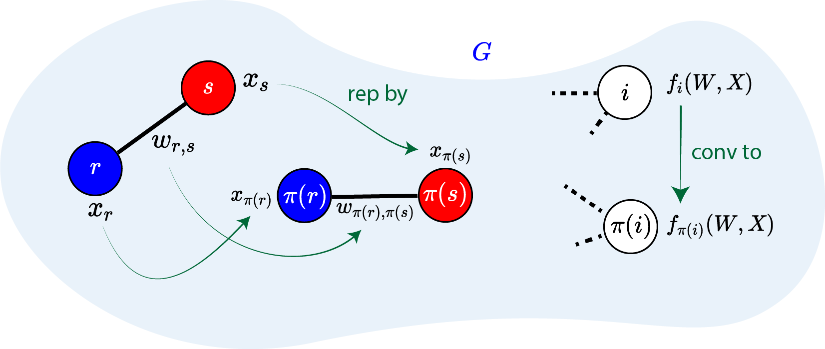
(a) Illustration of Condition (6).

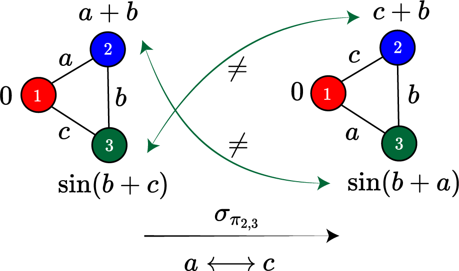
(b) Item 1 of Example 2.4

Figure 1: (a) Illustration of (6) which states that replacing all weights $w_{r,s}$ by $w_{\pi(r),\pi(s)}$ and all features $x_{r}$ by $x_{\pi(r)}$, converts $f_{i}(W,X)$ into $f_{\pi(i)}(W,X)\,$; (b) Showing that Item 1 of Example 2.4 fails to satisfy (6) for $\pi=\pi_{2,3}$. For simplicity we used $w_{1,2}=a$, $w_{2,3}=b$, and $w_{1,3}=c$.

To demonstrate the connection between permutation compatibility and GNNs, we start by the necessity result, which generalizes the previously-known results on the permutation invariancy of GNNs.

Theorem 3.2 (Necessity).

Suppose $H^{(k)}(W,X)$ is a GNN over $\mathcal{G}_{n,d}$. For any finite $k\geq 0$, the resulting $H^{(k)}$ is permutation compatible.

The above theorem can be formally proven by induction on $k$. We next proceed with sufficiency results which are far more challenging and, in some cases, require feature augmentation. Our first sufficiency result is restricted to graphs with distinct features.

Definition 3.3.

Define $\tilde{\mathcal{G}}_{n,d}$ to be the set of all graphs with distinct node features:

$$\tilde{\mathcal{G}}_{n,d}=\left\{G=([n],W,X)\in\mathcal{G}_{n,d}\mid X=(x_{1}^{\top},\ldots,x_{n}^{\top})\text{, where }x_{1},\ldots,x_{n}\text{ are distinct}\right\}.$$ (7)

Theorem 3.4 (Sufficiency for distinct features).

Suppose $F\in\mathcal{F}_{n,d}$. Then there exists a GNN $H^{(k)}$ with finite $k\geq 0$ such that $H^{(k)}(W,X)=F(W,X)$ for all $G=([n],W,X)\in\tilde{\mathcal{G}}_{n,d}$.

In the case where the features are identical, we show later in Section 5 that permutation compatibility of a graph function may no longer be sufficient to guarantee that it is generated by a GNN. We establish this result by making a connection with the 1-WL test. However, as we will show below, a simple augmentation scheme makes it possible to extend Theorem 3.4 to any permutation-compatible function.

Theorem 3.5 (Extending the sufficiency to arbitrary features).

Suppose $F\in\mathcal{F}_{n,d}$. For any graph $G=([n],W,X)\in\mathcal{G}_{n,d}$, let us augment the (row vector) features $x_{1},\ldots,x_{n}$ with arbitrary but distinct vectors, i.e., $x^{\ast}_{i}=(x_{i},y_{i})$, where $y_{1},\ldots,y_{n}\in\mathbb{R}^{d_{0}}$ are distinct. Let us denote the new feature matrix by $X^{\ast}=(x^{\ast\top}_{1},\ldots,x^{\ast\top}_{n})$. Then, there exists a GNN, i.e., $H^{(k)}$ with some finite $k\geq 0$ over $\mathcal{G}_{n,d+d_{0}}$, such that $H^{(k)}(W,X^{\ast})=F(W,X)$ for all $G=([n],W,X)\in\mathcal{G}_{n,d}$.

Theorem 3.4 and Theorem 3.5 are proven in Appendix D and Appendix E, respectively. However, we provide the sketch of the proof in Section 3.3.

3.1 Verification of Permutation-Compatible Functions

It is easy to see that naively verifying Condition (6) over all permutations leads to $n\cdot n!$ functional constraints. However, it turns out that these constraints can be equivalently represented by a subset of $n(n-1)/2$ constraints. This is because, at a high level, any permutation can be decomposed into a sequence of swaps of a pair of elements (a.k.a transpositions), and thus, invariancy on arbitrary permutations can be verified via the invariancy on transpositions. This results in the following theorem.

Proposition 3.6.

Consider a function $F=(f_{1},\ldots,f_{n})$ over $\mathcal{G}_{n,d}$. Then $F\in\mathcal{F}_{n,d}$ if and only if there exists $i_{0}\in[n]$ such that both of the following conditions hold for all $G=([n],W,X)\in\mathcal{G}_{n,d}$:

$$\text{For all }r,s\in[n]_{-i_{0}}:\quad f_{i_{0}}(\sigma_{\pi_{r,s}}(W),\lambda_{\pi_{r,s}}(X))=f_{i_{0}}(W,X).$$ (8)

$$\text{For all }j\in[n]_{-i_{0}}:\quad f_{j}(W,X)=f_{i_{0}}(\sigma_{\pi_{i_{0},j}}(W),\lambda_{\pi_{i_{0},j}}(X)).$$ (9)

In the next two subsections, we consider specific examples of graph functions and determine whether or not they satisfy the conditions stated in Proposition 3.6.

3.1.1 Permutation-Compatible Examples

Using Proposition 3.6 it is easy to verify that the functions given in Item 4 and Item 5 of Example 2.4 are permutation compatible. The following corollary provides cases for which verifying permutation-compatibility is even simpler than Proposition 3.6. We refer to Appendix G for more details.

Corollary 3.7 (Informal).

$F=(f_{1},\ldots,f_{n})$ is permutation compatible if any of the following holds:

(i) $F$ ignores $W$ and $f_{i}$ is invariant under any permutation of features $x_{j}\,$ for $j\neq i$,

(ii) $F$ assigns the same value to all $f_{i}$ and this value is invariant under any graph isomorphism.

Using Corollary 3.7 - part (i), we can immediately conclude that Items  2 and 3 of Example 2.4 are permutation-compatible functions. The implication of part (ii) is expressed in the following remark.

Remark 3.8.

Corollary 3.7- part (ii) implies that the min-cut value function given in Item 7 of Example 2.4 is permutation compatible and hence can be generated by a GNN using a distinct feature augmentation due to Theorem 3.5. Indeed, many classical graph problems such as the clique number and the max-flow value can be shown to be permutation compatible due to Corollary 3.7 - part (ii).

3.1.2 Permutation-Incompatible Examples

Consider the function $F$ defined in Item 1 of Example 2.4. We claim that $F\notin\mathcal{F}_{3,d}$, i.e., $F$ fails to satisfy (6). Let $\pi=\pi_{2,3}$, i.e., we have $\pi(1)=1,\pi(2)=3,\pi(3)=2$. Let $W^{\prime}=\sigma_{\pi}(W)$ and $X^{\prime}=\lambda_{\pi}(X)$. Note that $W^{\prime}$ consists of three elements $w^{\prime}_{1,2}$, $w^{\prime}_{1,3}$, and $w^{\prime}_{2,3}$ and $X^{\prime}=(x_{1}^{\prime},x_{2}^{\prime},x_{3}^{\prime})$. As shown in Figure 1-(b), under the permutation $\sigma_{\pi}$ on the weights, we get $w^{\prime}_{1,2}=w_{1,3}$, $w^{\prime}_{1,3}=w_{1,2}$, and $w^{\prime}_{2,3}=w_{2,3}$, and under $\lambda_{\pi}$ on the features, we get $x^{\prime}_{1}=x_{1}$, $x^{\prime}_{2}=x_{3}$, and $x^{\prime}_{3}=x_{2}$. We now apply $(\sigma_{\pi},\lambda_{\pi})$ on each node function as follows (note that the specific choice of $F$ considered here totally ignores $X$ and only depends on $W$):

$$f_{1}(\sigma_{\pi}(W),\lambda_{\pi}(X)) =f_{1}(W^{\prime},X^{\prime})=0,$$ (10)

$$f_{2}(\sigma_{\pi}(W),\lambda_{\pi}(X)) =f_{2}(W^{\prime},X^{\prime})=w^{\prime}_{1,2}+w^{\prime}_{2,3}=w_{1,3}+w_{2,3},$$ (11)

$$f_{3}(\sigma_{\pi}(W),\lambda_{\pi}(X)) =f_{3}(W^{\prime},X^{\prime})=\sin\left(w^{\prime}_{1,3}+w^{\prime}_{2,3}\right)=\sin\left(w_{1,2}+w_{2,3}\right).$$ (12)

Since $\pi(2)=3$, guaranteeing (6) requires $f_{3}(W,X)=f_{2}(\sigma_{\pi}(W),\lambda_{\pi}(X))$, which does not hold as $f_{3}(W,X)=\sin(w_{1,3}+w_{2,3})$ while $f_{2}(\sigma_{\pi}(W),\lambda_{\pi}(X))=w_{1,3}+w_{2,3}$. Hence, $F\notin\mathcal{F}_{3,d}$.

3.2 Permutation Compatibility and Node Labeling

In this section, we explain that permutation compatibility is a formal way of saying that a function is blind to node identities, i.e., fixing a node, the value that the function assigns to that node remains the same under re-labeling. To see this, pick a permutation $\pi\in S_{n}$ and re-label the nodes by writing $\pi^{-1}(i)$ instead of $i$. Therefore, the new label for the edge $\{i,j\}$ is now $\{\pi^{-1}(i),\pi^{-1}(j)\}$. Letting $W^{\prime}=\sigma_{\pi}(W)$ and $X^{\prime}=\lambda_{\pi}(X)$, note that $w_{\pi^{-1}(i),\,\pi^{-1}(j)}^{\prime}$ refers the weight of the edge whose new name is $\{\pi^{-1}(i),\pi^{-1}(j)\}$ and $x^{\prime}_{\pi^{-1}(i)}$ refers to the feature of the node whose name is $\pi^{-1}(i)$. Indeed, $w_{\pi^{-1}(i),\,\pi^{-1}(j)}^{\prime}=w_{\pi(\pi^{-1}(i)),\,\pi(\pi^{-1}(j))}=w_{i,j}$ and $x^{\prime}_{\pi^{-1}(i)}=x_{\pi(\pi^{-1}(i))}=x_{i}$. The original function value assigned to node $i$ was $f_{i}(W,X)$, and now under the re-labeling the value assigned to the same node (which is now named $\pi^{-1}(i)$) is $f_{\pi^{-1}(i)}(W^{\prime},X^{\prime})$. If $F$ does not depend on node labelings, these two values should be equal, i.e., $f_{\pi^{-1}(i)}(W^{\prime},X^{\prime})=f_{i}(W,X)$ or $f_{\pi^{-1}(i)}(\sigma_{\pi}(W),\lambda_{\pi}(X))=f_{i}(W,X)$ for all $i\in[n]$. Replacing $i=\pi(k)$ in this equation implies that $f_{k}(\sigma_{\pi}(W),\lambda_{\pi}(X))=f_{\pi(k)}(W,X)$ must hold for all $k$, which is the permutation-compatibility condition in (6).

3.3 Characterization of $\mathcal{F}_{n,d}$ and Proof Sketch

In this section, we study a characterization of $\mathcal{F}_{n,d}$ that paves the path for proving Theorem 3.4. Based on the definitions and results of this section, Theorem 3.4 is proven in Appendix D. To reach the result of Theorem 3.4, we take the following steps:

(i) Building MEF functions. We start by introducing the notion of multiset-equivalent functions (MEF) and provide useful candidates for such functions. MEFs are building blocks for defining the basis functions in step (ii).

Definition 3.9 (Multiset-Equivalent Function (MEF)).

For positive integers $n$ and $m$, we call the function $\psi:\mathbb{R}^{m}\to\mathbb{R}^{p}$ a multiset-equivalent function (MEF), if for all $v_{1},\ldots,v_{n},v_{1}^{\prime},\ldots,v_{n}^{\prime}\in\mathbb{R}^{m}$, the equation

$$\sum_{i=1}^{n}\psi\left(v_{i}\right)=\sum_{i=1}^{n}\psi\left(v_{i}^{\prime}\right),$$ (13)

holds if and only if there exists a permutation $\pi\in S_{n}$ such that $(v_{1}^{\prime},\ldots,v_{n}^{\prime})=(v_{\pi(1)},\ldots,v_{\pi(n)})$. For fixed $m$ and $n$, the class of all such functions is denoted by $\Psi_{m,n}$. Moreover, we refer to $p$, the dimension of the co-domain of the function $\psi$ as $p({\psi})$.

The summation of the function $\psi$ aims to generate an algebraic form for a multiset of vectors. Previous works [43, 35] developed ideas to translate multisets to functional forms. However, the approaches in these works cannot translate a multiset of “vectors” of arbitrary dimension to an algebraic summation which is required by Definition 3.9. In Proposition 3.10, we introduce candidate multiset-equivalent functions for every $m$ and $n$ to ensure that the existence of such functions and provide a constructive framework for the proofs in this paper. The term “multise” in MEF refers to a generalisation of a set in which repetition of elements is permitted (see Appendix A for a formal definition of a multiset). The name multiset-equivalent function for $\psi$ in Definition 3.9, relates to the fact that the summation of $\psi$ over a sequence of vectors preserves all the data up to a permutation and thus this sum is equivalent to the “multiset” of data. It is not trivial to find an MEF. For instance, note that the identity function (which leads to $\sum_{i=1}^{n}v_{i}=\sum_{i=1}^{n}v_{i}^{\prime}$) is not an MEF for $n>1$. This is because when $m=1$ and $n=2$, we have $2+5=3+4$ but $(2,5)$ is not a permutation of $(3,4)$. A natural question here is whether such function exists at all. The following proposition introduces candidate elements of $\Psi_{m,n}$ for all positive integers $n$ and $m$.

Proposition 3.10.

The followings are specific constructions of MEFs for (i) $m=1$, and (ii) $m>1$:

1. Consider the function $\psi:\mathbb{R}\to\mathbb{R}^{n}$ such that for $v\in\mathbb{R}$, $\psi(v)=(v,v^{2},\ldots,v^{n})$. Then $\psi\in\Psi_{1,n}$. Moreover, note that $p(\psi)=n$.

2. Let $m>1$ and consider $v=(v_{1},\ldots,v_{m})\in\mathbb{R}^{m}$. Define $\psi(v)=\psi(v_{1},\cdots,v_{m})$ to be an $n\times m\times m$ array (tensor) with real elements such that for every $\ell\in[n]$ and $r,s\in[m]$ with $r<s$:

   $$[\psi(v_{1},\cdots,v_{m})]_{\ell,r,s} =\operatorname{Re}\left(\left(v_{r}+v_{s}\sqrt{-1}\right)^{\ell}\right),$$ (14)

   $$[\psi(v_{1},\cdots,v_{m})]_{\ell,s,r} =\operatorname{Im}\left(\left(v_{r}+v_{s}\sqrt{-1}\right)^{\ell}\right).$$ (15)

   Note that $\psi(v)\in\mathbb{R}^{n\times m\times m}$. Let us re-shape $\psi(v)$ into a long vector in $\mathbb{R}^{m^{2}n}$, and consider $\psi:\mathbb{R}^{m}\to\mathbb{R}^{m^{2}n}$. Then $\psi\in\Psi_{m,n}$. Moreover, note that $p(\psi)=m^{2}n$.

To construct valid MEFs, the idea behind this specific choice of $\psi$ in Proposition 3.10 for $m=1$ is that when we take the sum $\psi$ over $n$ scalars, it encodes them into the roots of a unique polynomial and thus it preserves the data up to a permutation. For $m>1$, this idea is extended by encoding vectors of arbitrary size into the roots of a system of complex polynomials. See the proof in Appendix H.

(ii) Constructing a basis function based on MEFs. In the following definition, we construct a graph function over $\mathcal{G}_{n,d}$ through MEFs which we call a basis function.

Definition 3.11 (Basis Function).

Define the graph function $\mathcal{B}=(\beta_{1},\ldots,\beta_{n})$ over $\mathcal{G}_{n,d}$ such that for $i\in[n]$:

$$\beta_{i}\left(W,X\right)=\left(x_{i},\sum_{j\in[n]_{-i}}\psi_{2}\left(x_{j},w_{i,j},\sum_{\ell\in[n]_{-j}}\psi_{1}\left(x_{\ell},w_{j,\ell}\right)\right)\right),$$ (16)

where $\psi_{1}\in\Psi_{d+1,n-1}$ and $\psi_{2}\in\Psi_{p(\psi_{1})+d+1,n-1}$ is the same for all $i\in[n]$. We call $\mathcal{B}$ a basis function over $\mathcal{G}_{n,d}$.

This specific structure of a basis function leads to an important property which is stated and formally proven in the following proposition.

Proposition 3.12.

Let $\mathcal{B}=(\beta_{1},\ldots,\beta_{n})$ be a basis function over $\mathcal{G}_{n,d}$. Then $\mathcal{B}\in\mathcal{F}_{n,d}$ with the following additional property: Given two graphs $G=([n],W,X)$ and $G^{\prime}=([n],W^{\prime},X^{\prime})$ in $\tilde{\mathcal{G}}_{n,d}$, for every $i\in[n]$, if $\beta_{i}(W,X)=\beta_{i}(W^{\prime},X^{\prime})$, then there exists $\pi\in\nabla_{i}$ such that $W^{\prime}=\sigma_{\pi}(W)$ and $X^{\prime}=\lambda_{\pi}(X)$.

The fact that $\psi_{1}$ and $\psi_{2}$ are MEFs is crucial in showing that the specific structure of the basis function in (16) leads to Proposition 3.12. We omit the details here and refer to the proof of Proposition 3.12 in Appendix I.

(iii) Representing any permutation-compatible function in terms of the basis function. The key property of $\beta_{i}$ mentioned in part (ii) enables us to represent any permutation-compatible function $F$ in terms of the basis function. This is formalized in the following theorem.

Theorem 3.13 (Main Representation Theorem).

Suppose $F\in\mathcal{F}_{n,d}$ with $F=(f_{1},\ldots,f_{n})$ and let $\mathcal{B}=(\beta_{1},\ldots,\beta_{n})$ be a basis function over $\mathcal{G}_{n,d}$ and recall $\tilde{\mathcal{G}}_{n,d}$ from Definition 3.3. Then, there exists a function $\rho$ s.t. for every $i\in[n]$ and $G=([n],W,X)\in\tilde{\mathcal{G}}_{n,d}$, we have $f_{i}(W,X)=\rho(\beta_{i}(W,X))$.

Theorem 3.13 states that any node function $f_{i}$ of a permutation-compatible function $F$ can be written in terms of $\beta_{i}$ over the set of graphs with distinct features $\tilde{\mathcal{G}}_{n,d}$ defined in Definition 3.3. Theorem 3.13 is an equivalent way of saying that subject to having distinct node features in a graph, $\beta_{i}(W,X)=\beta_{i}(W^{\prime},X^{\prime})$ leads to $f_{i}(W,X)=f_{i}(W^{\prime},X^{\prime})$.

(iv) Constructing the GNN. Using the Representation Theorem 3.13, to generate $F$, it suffices to construct a GNN such that $h_{i}^{(k)}(W,X)=\rho(\beta_{i}(W,X))$. Due to the construction of $\beta_{i}$ in (16), a GNN can generate it in two iterations. Using $\rho$ in the third iteration then completes the construction. More formally, we set candidates for $\phi_{1}$, $\phi_{2}$, and $\phi_{3}$ (defined in (4)) as follows:

$$\phi_{1}\left(h_{j}^{(0)},h_{\ell}^{(0)},w_{j,\ell}\right)=\left(\frac{1}{n-1}h_{j}^{(0)},\,\,\psi_{1}\left(h_{\ell}^{(0)},w_{j,\ell}\right)\right),$$ (17)

$$\phi_{2}\left(h_{i}^{(1)},h_{j}^{(1)},w_{i,j}\right)=\left(\frac{1}{n-1}\left[h_{i}^{(1)}\right]_{1:d},\psi_{2}\left(\left[h_{j}^{(1)}\right]_{1:d},w_{i,j},\left[h_{j}^{(1)}\right]_{d+1:d+p(\psi_{1})}\right)\right),$$ (18)

$$\phi_{3}\left(h_{i}^{(2)},h_{j}^{(2)},w_{i,j}\right)=\frac{1}{n-1}{\rho\left(h_{i}^{(2)}\right)}.$$ (19)

In Equation 18, the notation $[v]_{a:b}$ for $v=(v_{1},\ldots,v_{m})$ means $[v]_{a:b}=(v_{a},v_{a+1},\ldots,v_{b})$. It is straightforward to see that $h_{i}^{(2)}(W,X)=\beta_{i}(W,X)$ and $h_{i}^{(3)}(W,X)=\rho(\beta_{i}(W,X))$. This results in $h_{i}^{(3)}(W,X)=f_{i}(W,X)$ for all $G=([n],W,X)\in\tilde{\mathcal{G}}_{n,d}$, due to Theorem 3.13.

The steps (i) to (iv) provide a proof sketch for Theorem 3.4 which is the main stand to reach the other results in this paper. At the heart of this analysis lies Theorem 3.13 which has other theoretical benefits. For example, one might ask if we can generate a continuous permutation-compatible graph function by using continuous $\phi_{k}$’s in the GNN? In particular, answering this question is useful when one chooses $\phi_{k}$ from the class of multi-layer perceptrons (MLPs) as good approximates for continuous functions. The following result provides an answer.

Corollary 3.14.

Considering Theorem 3.4, if $F(W,X)$ is continuous with respect to $(W,X)$, then a GNN $H^{(k)}$ with continuous inner functions $\phi_{k}$ exists that works for the theorem.

4 Feature Crafting to Generate All Graph Functions

In this section, we discuss how GNNs can go beyond permutation compatibility and generate any graph function. In brief, we show that if we augment the identity of each node $i$ to its associated feature $x_{i}$, i.e. set $\tilde{x}_{i}=(x_{i},i)$, and let $\tilde{X}$ be the concatenation of $\tilde{x}_{i}\,$s, then for any graph function $F(W,X)$, a GNN exists that receives $W$ and $\tilde{X}$ and outputs $F(W,X)$.

Theorem 4.1.

Suppose $n$ fixed distinct vectors $y_{1},\ldots,y_{n}\in\mathbb{R}^{d_{0}}$ are given and we augment them to features of all graphs. More formally, for every $G=([n],W,X)\in\mathcal{G}_{n,d}$ with feature matrix $X=(x_{1}^{\top},\ldots,x_{n}^{\top})$, we augment $y_{i}$ to the feature $x_{i}$ to construct $\tilde{x}_{i}=(x_{i},y_{i})\in\mathbb{R}^{d+d_{0}}$ for all $i\in[n]$. One simple option is $d_{0}=1$ and $(y_{1},\ldots,y_{n})=(1,\ldots,n)$. Let $\tilde{X}=(\tilde{x}_{1}^{\top},\ldots,\tilde{x}_{n}^{\top})$. Then for every graph function $F(W,X)$, there exists a GNN $H^{(k)}$ with a finite $k\geq 0$ over $\mathcal{G}_{n,d+d_{0}}$ such that $H^{(k)}(W,\tilde{X})=F(W,X)$ for all $G=([n],W,X)\in\mathcal{G}_{n,d}$.

The proof of Theorem 4.1 is built on the framework of basis functions described in Section 3.3. In brief, the basis function output $\beta_{i}(W,\tilde{X})$ uniquely determines the triple $(W,X,i)$ and thus a GNN can achieve any graph function as the next step after generating $\beta_{i}(W,\tilde{X})$.

How do the augmentations in Theorem 3.5 and Theorem 4.1 differ? We described two types of augmentation in Theorem 3.5 and Theorem 4.1 which we call soft-coded and hard-coded augmentation, respectively. In both cases, distinct nodes in a graph receive distinctly augmented values. However, in the hard-coded case, a fixed and unique value is augmented to the feature of node $i$ for all the graphs in $\mathcal{G}_{n,d}$, while this is not necessarily the case for a soft-coded augmentation. This difference can be stated in logical terms as follows:

$$\text{hard-coded}: \quad\exists y_{1},\ldots,y_{n}\quad\forall G\in\mathcal{G}_{n,d}\quad\text{$G$ is augmented by $y_{i}\,$s,}$$ (20)

$$\text{soft-coded}: \quad\forall G\in\mathcal{G}_{n,d}\quad\exists y_{1},\ldots,y_{n}\quad\text{$G$ is augmented by $y_{i}\,$s}.$$ (21)

To see the computational difference between these two augmentations, consider the example illustrated in Figure 2 -(a) and (b). In each of the Figure 2 -(a) and (b), the right graph is obtained by swapping the labels $1$ and $2$ in the left graph. A hard-coded augmentation means $(y_{1},y_{2},y_{3},y_{4})=(1,2,3,4)$ for both labelings of the graph. This is sensitive to node labeling. In other words, omitting the node labels, one sees two different sets of node features for the same graph in Figure 2 -(b). In contrast, under a soft-coded augmentation, we can have $(y_{1},y_{2},y_{3},y_{4})=(1,2,3,4)$ for the left graph in Figure 2 -(a) and $(y_{1},y_{2},y_{3},y_{4})=(2,1,3,4)$ for the right graph. Unlike the hard-coded augmentation, by ignoring the labels, we see the same set of node features for the same graph. Hence, the soft-coded augmentation can be set independently of node labeling. This elaboration reveals that, under a hard-coded augmentation, building a full dataset for training the GNN needs potentially $n!$ samples corresponding to all the $n!$ possible labelings of the same graph. This is the same cost when one treats a graph data as a matrix pair $(W,X)$ and gives it to an ordinary feed-forward neural net, ignoring the graph-based structure of the GNN.

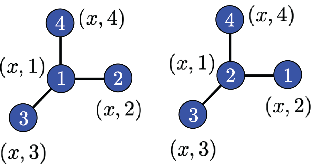
(a) Soft-coded

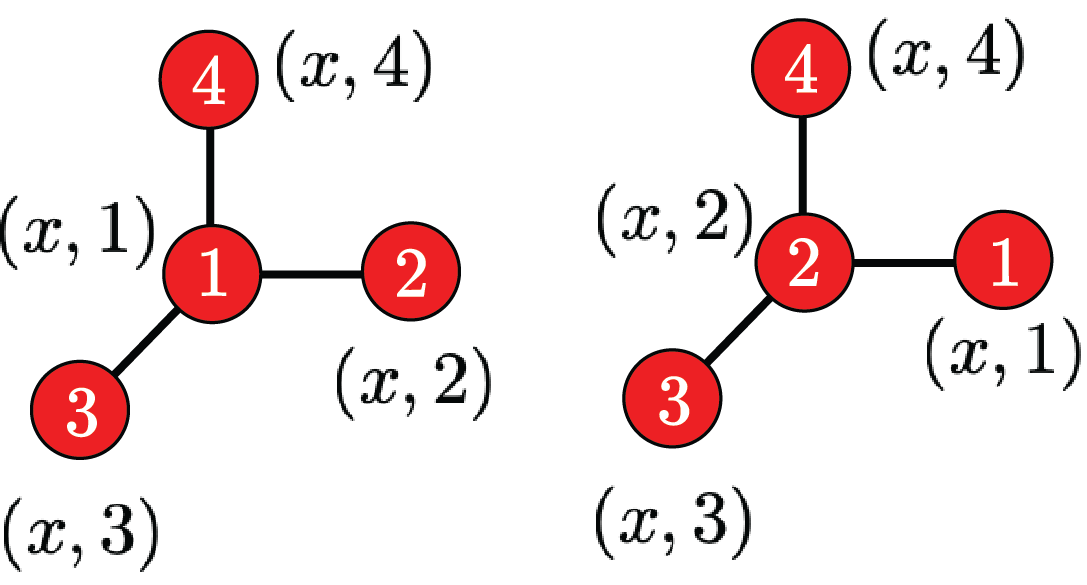
(b) Hard-coded

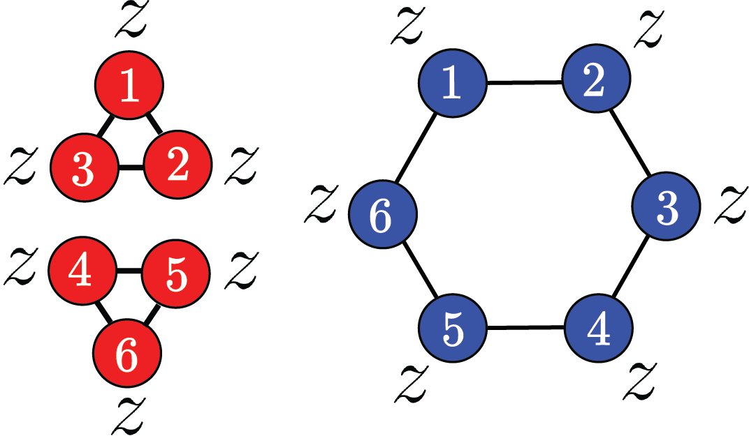
(c) Identical labels

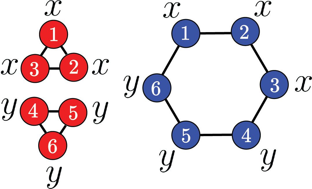
(d) Non-identical labels.

Figure 2: (a) and (b): The difference between the soft-coded and hard-coded augmentations. (c) and (d): Illustration of the hexagon versus the two-triangle graph, where 1-WL cannot separate between the two under identical labels (c) and can separate them under non-identical labels (d).

From Section 3.2, permutation compatibility translates into independency from node identities. Moreover, we know that hard-coded augmentation essentially means revealing node identities to the GNN. In this way, Theorem 4.1 requires revealing all the node identities to the GNN via a hard-coded augmentation. From the discussion above, we know that this is costly. Now the question is: In the case that $F$ depends only on a subset of node identities, can we use a hard-coded augmentation only on that subset of nodes instead of all the nodes? The following informally-stated corollary gives a positive answer. We will see the implications of this result on the shortest-path problem later in Section 6.1. For a formal statement and proof, we refer to Appendix M.

Corollary 4.2 (Informal).

Suppose a graph function $F$ does not depend on the node labels except for $i_{1},\ldots,i_{k}\in[n]$, i.e., (6) holds for every $\pi\in S_{n}$ that satisfies $\pi(j)=j$ for $j\in\{i_{1},\ldots,i_{k}\}$. Then $F$ can be generated by a GNN under a hard-coded augmentation for $i_{1},\ldots,i_{k}$ and a soft-coded augmentation for other nodes.

5 Weisfeiler-Lehman Test Versus GNN

Recent works [35, 21] have explained the expressiveness of GNNs via the Weisfeiler-Lehman (WL) isomorphism test. We now discuss the connection between permutation compatibility and WL test.

Starting with all nodes of identical labels/colors, the 1-WL test iteratively and through message passing assigns new labels to nodes in the form of multi-sets. If at any iteration of the procedure, the labeling of two graphs differ, they are certainly not isomorphic. However, it can very well happen that the 1-WL test produces the same labeling at every single iteration while the two graphs are not isomorphic, e.g., the hexagon and the two-triangle graph shown in Figure 2-(c). Similarly, a GNN that aims to compute the min-cut function (an instance of a permutation-compatible function) produces the same value for both graphs if it starts with identical node features. In fact, this is a general phenomenon: if the 1-WL fails then a permutation-compatible function with identical features cannot be generated by a GNN. To formalize this equivalency, which is essentially the same result as in [35, 21], we need to set a notation for graphs under identical node features and also a formal proof in our general setting. To this end, consider the following definition.

Definition 5.1.

Fix a constant vector $c\in\mathbb{R}^{d}$. Let us define

$$\mathcal{G}^{c}_{n,d}=\left\{G=([n],W,C)\in\mathcal{G}_{n,d}\mid W\in\{0,1\}^{n\times n},C=(c^{\top},\ldots,c^{\top})\right\}.$$

Moreover, we need to precisely define what it means that a GNN can not separate between two graphs. The following definition specifies this notion using the notation $\#\{\cdot\}$. This notation refers to a multiset of elements. A multiset generalizes the concept of a set by allowing the repetition of elements. For a formal definition, we refer to Appendix A.

Definition 5.2.

Suppose $G_{1},G_{2}\in\mathcal{G}_{n,d}$, with $G_{1}=([n],W_{1},X_{1})$ and $G_{2}=([n],W_{2},X_{2})$. We say that GNNs over $\mathcal{G}_{n,d}$ cannot separate $G_{1}$ and $G_{2}$ if for every $k\geq 0$ and every GNN $H^{(k)}=(h_{1}^{(k)},\ldots,h_{n}^{(k)})$, we have $\#\{h_{i}^{(k)}(W_{1},X_{1})\mid i\in[n]\}=\#\{h_{i}^{(k)}(W_{2},X_{2})\mid i\in[n]\}$.

The following result formalises the earlier statement.

Proposition 5.3.

Suppose $G_{1},G_{2}\in\mathcal{G}^{c}_{n,d}$ are graphs without isolated nodes. Then GNNs over $\mathcal{G}^{c}_{n,d}$ cannot separate $G_{1}$ and $G_{2}$ if and only if 1-WL cannot distinguish between $G_{1}$ and $G_{2}$.

In light of the above theorem, feature augmentation for GNNs in general is unavoidable as there are permutation compatible functions (such as min-cut) that cannot be generated by any GNN under identical node features.

6 Dynamic Programming Versus GNN

Dynamic Programming (DP) is an iterative mechanism that evolves the state of some entities by starting at initial states and updating the current state of each entity as a function of the current state of others. Treating $h_{i}^{(k)}$ as the state of node $i$ in the $k$-the iteration, GNNs also lie in this category. Therefore, one would expect a close connection between GNN and DP. One possible approach to explain the connection between GNN and DP is to quantify the connection between their iterative structure [37, 6, 31]. However, our results are of different nature. For any algorithmic procedure on graph, DP or otherwise, for which there is an output graph function $F$, we discuss how GNNs can generate $F$. Due to Theorem 4.1, this is possible for any graph function $F$. The only thing to consider further is that if $F$ is permutation compatible or if it depends on identity of only a subset of nodes (as formalised in Corollary 4.2), we can avoid the costly hard-coded augmentation of Theorem 4.1 and use Theorem 3.5 or Corollary 4.2 instead. Hence, given $F_{\operatorname{DP}}(W,X)$ as the output of a DP, based on whether $F_{\operatorname{DP}}$ is permutation compatible or otherwise, we can generate it under a proper augmentation using Theorem 3.5, Theorem 4.1, and Corollary 4.2. As a particular example, let us explain the situation for the shortest path problem in Section 6.1.

6.1 Shortest-Path-Length Problem

In connection with DP, in this section, we consider the shortest-length problem as the output of the Bellman-Ford dynamic program. We show that GNNs are able to generate the shortest-path-length function to a source node as long as the source node is identified through the node features. This identification of the source node is trivially required by any algorithm. For a formal argument, consider the distance-to-node-$1$ function $F$ in Item 6 of Example 2.4. Note that $F$ is not permutation compatible since it does not necessarily satisfy (6) for a $\pi$ with $\pi(1)\neq 1$. However, (6) is satisfied over all permutations $\pi$ s.t. $\pi(1)=1$. This is formalised in the following lemma.

Lemma 6.1.

Let $F(W,X)$ be the distance-to-node-1 function defined in Item 6 of Example 2.4. Since $F(W,X)$ ignores $X$, we use the notation $F(W)=(f_{1}(W),\ldots,f_{n}(W))$. Then for every $\pi\in\nabla_{1}$ and $i\in[n]$, we have $f_{\pi{(i)}}(W)=f_{i}(\sigma_{\pi}(W))$ for every weight matrix $W$.

Based on Lemma 6.1, Corollary 4.2 implies that hard-coded augmentation is only needed on node $1$ to generate the $F$ which equivalently means revealing the identity of node $1$ to the GNN. Corollary 4.2 also requires a soft-coded augmentation on other nodes. The latter, however, turns out to be unnecessary due to following proposition which summarises our results on the shortest path problem.

Proposition 6.2 (Informal).

Letting $F(W)$ to be the distance-to-node-1 function, (i) $F$ is not permutation compatible. (ii) Using a fixed feature matrix $X_{0}=(y_{1},\ldots,y_{n})$ for all graphs, a GNN can generate $F$ if and only if $y_{1}$ is distinct from other $y_{i}\,$s.

See Appendix P for a formal statement and proof. Note that $X_{0}=(1,0,\ldots,0)$ works well for Proposition 6.2 while for example $X_{0}=(1,1,0,\ldots,0)$ fails. The latter is intuitively trivial since it gives no clue to the GNN in identifying the source node.

Conclusion

In this paper, we provided an analytic framework to study the representation power of GNNs. We introduced the fundamental notion of permutation compatibility that fully characterizes what graph functions may (or may not) be generated by a GNN.

Appendix A Preliminaries for appendices

Notation. We denote by $f\circ g$, the composition of functions $f$ and $g$, meaning that $f\circ g(x)=f(g(x))$. Moreover, for a vector $v=(v_{1},\ldots,v_{m})$, let $[v]_{a:b}$ for $a\leq b$, denote the sub-vector consisting of the elements with indices starting from $a$ to $b$, that is, $[v]_{a:b}=(v_{a},v_{a+1},\ldots,v_{b})$. In this notation, we also use “end” to refer to the last index, i.e., $[v]_{a:\text{end}}=[v]_{a:m}$.

In the following, we provide formal definitions that are used in the proofs. We start by the formal definition of a multiset.

Definition A.1 (Multiset).

Multisets generalize the concept of a set in which the repetition of elements is allowed. A multiset is a pair $Y=(S,m)$, where $S$ is the underlying set of the distinct elements of $Y$ and $m:S\to\mathbb{Z}_{\geq{1}}$ is the function that indicates the multiplicity of each element.

For the ease of explanation, we set the following notation for a multiset.

Definition A.2 (Notation $\#\{\cdot\}$).

Suppose $y_{1},\ldots,y_{n}$ are some objects with possibly repeated elements, then the multiset containing $y_{1},\ldots,y_{n}$ is denoted by $\#\{y_{1},\ldots,y_{n}\}$. More formally, if the set of distinct elements among $y_{1},\ldots,y_{n}$ is $\{y_{i_{1}},\ldots,y_{i_{r}}\}$ with $m(y_{i_{1}}),\ldots,m(y_{i_{n}})$ denoting the multiplicity of the elements, then

$$\#\{y_{1},\ldots,y_{n}\}=(\{y_{i_{1}},\ldots,y_{i_{r}}\},m).$$ (22)

The notation $\#\{\cdot\}$ considers the repetition but ignores the order of the elements. Therefore, for the sequences $(y_{1},\ldots,y_{n})$ and $(z_{1},\ldots,z_{m})$ of possibly repeated elements, the equation

$$\#\{y_{1},\ldots,y_{n}\}=\#\{z_{1},\ldots,z_{m}\}$$ (23)

holds if and only if $m=n$ and there exists a permutation $\pi\in S_{n}$ such that $\left(y_{1},\ldots,y_{n}\right)=\left(z_{\pi(1)},\ldots,z_{\pi(n)}\right)$.

Appendix B Formal statement and proof of Proposition 2.6

To formalise a GNN with aggregator operator (5), we define the Extended-GNN analogous to Definition 2.5 as follows.

Definition B.1 (Extended-GNN).

An Extended Graph Neural Network (Extended-GNN) is an iterative mechanism that generates a sequence of functions $E^{(k)}$, $k\geq 0$, over $\mathcal{G}_{n,d}$ in the following manner. For $G=([n],W,X)\in\mathcal{G}_{n,d}$, the function $E^{(k)}(W,X)=(e_{1}^{(k)}(W,X),\ldots,e_{n}^{(k)}(W,X))$ is given as

$$\text{if }k=0:\,e_{i}^{(0)}=x_{i},$$ (24)

$$\text{if }k\geq 1:\,e_{i}^{(k)}=\Phi_{k}\left(e_{i}^{(k-1)},\#\left\{(e_{j}^{(k-1)},w_{i,j})\mid j\in[n]_{-i}\right\}\right),$$ (25)

for some functions $\Phi_{k},\,k\geq 1$, where for each $k$, the outputs of $\Phi_{k}$ lie in some Euclidean vector space.

Proposition B.2 (Formal).

The function-class of GNNs is equivalent to the function-class of Extended-GNNs. More formally, suppose a graph function $F$ over $\mathcal{G}_{n,d}$ is given. Then, there exists a GNN, denoted by $H^{(k^{\prime})}$, over $\mathcal{G}_{n,d}$ such that $H^{(k^{\prime})}(W,X)=F(W,X)$ for all $G=([n],W,X)\in\mathcal{G}_{n,d}$ if and only if there exists an Extended-GNN $E^{(k)}$ over $\mathcal{G}_{n,d}$ such that $E^{(k)}(W,X)=F(W,X)$ for all $G=([n],W,X)\in\mathcal{G}_{n,d}$.

Proof of Proposition B.2.

First note that the aggregator (4) is a special case of (25). Therefore, the GNN defined in Definition 2.5 is a special case of the Extended-GNN defined in Definition B.1 and thus one side of the claim is immediate. To prove the other direction, suppose an Extended-GNN $E^{(k)}(W,X)$ over $G_{n,d}$ is given. We show that there exists a GNN $H^{(k^{\prime})}(W,X)$ such that for every $r\geq 0$: $E^{(r)}(W,X)=H^{(2r)}(W,X)$ for all $G=([n],W,X)\in\mathcal{G}_{n,d}$. To this end, let us set some notations. Consider $E^{(k)}=(e_{1}^{(k)},\ldots,e_{n}^{(k)})$ and suppose the outputs of $e_{i}^{(k)}$ lie in $\mathbb{R}^{\alpha_{k}}$ for some $\alpha_{k}$ and fix multiset-equivalent functions (MEFs) $\psi_{k}\in\Psi_{\alpha_{k-1}+1,n-1}$, defined in Definition 3.9. Also note that candidates for MEFs are provided in Proposition 3.10.

As the first step, we claim that for all $k\geq 1$, there exists a function $\Theta_{k}$ such that

$$\Phi_{k}\left(e_{i}^{(k-1)},\#\left\{(e_{j}^{(k-1)},w_{i,j})\mid j\in[n]_{-i}\right\}\right)=\Theta_{k}\left(e_{i}^{(k-1)},\sum_{j\in[n]_{-i}}\psi_{k}\left(e_{j}^{(k-1)},w_{i,j}\right)\right).$$ (26)

To prove (26), it suffices to show that having

$$\left(e_{i}^{(k-1)},\sum_{j\in[n]_{-i}}\psi_{k}\left(e_{j}^{(k-1)},w_{i,j}\right)\right)=\left(\hat{e}_{i}^{(k-1)},\sum_{j\in[n]_{-i}}\psi_{k}\left(\hat{e}_{j}^{(k-1)},\hat{w}_{i,j}\right)\right)$$ (27)

leads to

$$\Phi_{k}\left(e_{i}^{(k-1)},\#\left\{(e_{j}^{(k-1)},w_{i,j})\mid j\in[n]_{-i}\right\}\right)=\Phi_{k}\left(\hat{e}_{i}^{(k-1)},\#\left\{(\hat{e}_{j}^{(k-1)},\hat{w}_{i,j})\mid j\in[n]_{-i}\right\}\right).$$ (28)

To show that (27) leads to (28), note that from (27), we have $e_{i}^{(k-1)}=\hat{e}_{i}^{(k-1)}$, and

$$\sum_{j\in[n]_{-i}}\psi_{k}\left(e_{j}^{(k-1)},w_{i,j}\right)=\sum_{j\in[n]_{-i}}\psi_{k}\left(\hat{e}_{j}^{(k-1)},\hat{w}_{i,j}\right).$$ (29)

Having (29), the definition of an MEF (see Definition 3.9) implies that

$$\#\left\{(e_{j}^{(k-1)},w_{i,j})\mid j\in[n]_{-i}\right\}=\#\left\{(\hat{e}_{j}^{(k-1)},\hat{w}_{i,j})\mid j\in[n]_{-i}\right\}.$$ (30)

Equation 30 together with $e_{i}^{(k-1)}=\hat{e}_{i}^{(k-1)}$ proves (28). Hence, we showed the existence of the function $\Theta_{k}$ satisfying (26).

Next, we construct a GNN to generate a given Extended-GNN $E^{(k)}$, using the function $\Theta_{k}$ introduced above. To this end, given an Extended-GNN $E^{(k)}=(e_{1}^{(k)},\ldots,e_{n}^{(k)})$, we construct a GNN $H^{(k^{\prime})}=(h_{1}^{(k^{\prime})},\ldots,h_{n}^{(k^{\prime})})$ such that $h_{i}^{(2r)}=e_{i}^{(r)}$ for all $r\geq 0$ and $i\in[n]$. This construction is as follows: For $r\geq 1$, set

$$\phi_{2r-1}\left(h_{i}^{(2r-2)},h_{j}^{(2r-2)},w_{i,j}\right) =\left(\frac{1}{n-1}h_{i}^{(2r-2)},\psi_{r}\left(h_{j}^{(2r-2)},w_{i,j}\right)\right),$$ (31)

$$\phi_{2r}\left(h_{i}^{(2r-1)},h_{j}^{(2r-1)},w_{i,j}\right) =\frac{1}{n-1}\Theta_{r}\left(h_{i}^{(2r-1)}\right).$$ (32)

Due to (31) and (32), for all $i\in[n]$, we have

$$h_{i}^{(2r-1)} =\sum_{j\in[n]_{-i}}\phi_{2r-1}\left(h_{i}^{(2r-2)},h_{j}^{(2r-2)},w_{i,j}\right)=\left(h_{i}^{(2r-2)},\sum_{j\in[n]_{-i}}\psi_{r}\left(h_{j}^{(2r-2)},w_{i,j}\right)\right),$$ (33)

$$h_{i}^{(2r)} =\sum_{j\in[n]_{-i}}\frac{1}{n-1}\Theta_{r}\left(h_{i}^{(2r-1)}\right)=\Theta_{r}\left(h_{i}^{(2r-2)},\sum_{j\in[n]_{-i}}\psi_{r}\left(h_{j}^{(2r-2)},w_{i,j}\right)\right).$$ (34)

Now, using the relation between $\Theta_{r}$ and $\Psi_{r}$ in (26), we conclude from (34) that

$$h_{i}^{(2r)}=\Phi_{r}\left(h_{i}^{(2r-2)},\#\left\{(h_{j}^{(2r-2)},w_{i,j})\mid j\in[n]_{-i}\right\}\right).$$ (35)

Next, we claim that $h^{(2r)}_{i}=e_{i}^{(r)}$ for all $r\geq 0$ and $i\in[n]$. We prove this by induction on $r$. For $r=0$, we have $h^{(0)}_{i}=e_{i}^{(0)}=x_{i}$. Given the induction hypothesis for $r-1$, we have $h^{(2r-2)}_{i}=e_{i}^{(r-1)}$ for all $i\in[n]$. Replacing this into (35) leads to

$$h_{i}^{(2r)}=\Phi_{r}\left(e_{i}^{(r-1)},\#\left\{(e_{j}^{(r-1)},w_{i,j})\mid j\in[n]_{-i}\right\}\right)=e_{i}^{(r)}.$$ (36)

Hence, we have $E^{(r)}(W,X)=H^{(2r)}(W,X)$ for all $r\geq 0$ and all $G=([n],W,X)\in\mathcal{G}_{n,d}$. ∎

Appendix C Proof of Theorem 3.2

Proof.

Consider a GNN $H^{(k)}=(h_{1}^{(k)},\ldots,h_{n}^{(k)})$ for some $k\geq 0$ over $\mathcal{G}_{n,d}$. We want to show that $H^{(k)}\in\mathcal{F}_{n,d}$. To this end, we must show that for every given $\pi\in S_{n}$, the following holds for all $G=([n],W,X)\in\mathcal{G}_{n,d}$ and all $i\in[n]$:

$$h_{\pi(i)}^{(k)}(W,X)=h_{i}^{(k)}\left(\sigma_{\pi}(W),\lambda_{\pi}(X)\right).$$ (37)

We prove (37) by induction on $k$. For $k=0$, we have $h_{i}^{(0)}(W,X)=x_{i}$ for all $i\in[n]$. Hence,

$$h_{i}^{(0)}\left(\sigma_{\pi}(W),\lambda_{\pi}(X)\right)=x_{\pi(i)}=h_{\pi(i)}^{(0)}\left(W,X\right).$$ (38)

Given the induction hypothesis for $k-1$, we must show that (37) holds for $k$. From (4), we have

$$h_{\pi(i)}^{(k)}(W,X) =\sum_{\ell\in[n]_{-\pi(i)}}\phi_{k}\left(h_{\pi(i)}^{(k-1)}\left(W,X\right),h_{\ell}^{(k-1)}\left(W,X\right),w_{\pi(i),\ell}\right)$$ (39)

$$=\sum_{j\in[n]_{-i}}\phi_{k}\left(h_{\pi(i)}^{(k-1)}\left(W,X\right),h_{\pi(j)}^{(k-1)}\left(W,X\right),w_{\pi(i),\pi(j)}\right)$$ (40)

$$=\sum_{j\in[n]_{-i}}\phi_{k}\left(h_{i}^{(k-1)}\left(\sigma_{\pi}(W),\lambda_{\pi}(X)\right),h_{j}^{(k-1)}\left(\sigma_{\pi}(W),\lambda_{\pi}(X)\right),w_{\pi(i),\pi(j)}\right),$$ (41)

where equation (40) is obtained by putting $j=\pi^{-1}(\ell)$ or equivalently $\ell=\pi(j)$ (note that any permutation is bijective by definition). Moreover, Equation 41 holds due to the induction hypothesis for $k-1$. By letting $W^{\prime}=\sigma_{\pi}(W)$ and $X^{\prime}=\lambda_{\pi}(X)$, we note that $w_{i,j}^{\prime}=w_{\pi(i),\pi(j)}$. Replacing these values in (41) results in

$$h_{\pi(i)}^{(k)}(W,X) =\sum_{j\in[n]_{-i}}\phi_{k}\left(h_{i}^{(k-1)}\left(W^{\prime},X^{\prime}\right),h_{j}^{(k-1)}\left(W^{\prime},X^{\prime}\right),w_{i,j}^{\prime}\right)=h_{i}^{(k)}\left(W^{\prime},X^{\prime}\right).$$ (42)

This concludes the induction and hence (37) is proven. As a result, $H^{(k)}\in\mathcal{F}_{n,d}$. ∎

Appendix D Proof of Theorem 3.4

Proof.

Suppose $F\in\mathcal{F}_{n,d}$ and let $F(W,X)=(f_{1}(W,X),\ldots,f_{n}(W,X))$. Consider a basis function $\mathcal{B}(W,X)=(\beta_{1}(W,X),\ldots,\beta_{n}(W,X))$ over $\mathcal{G}_{n,d}$ as defined in Definition 3.11. Due to Theorem 3.13, we can conclude that there exists a function $\rho$ such that for every $i\in[n]$, the following holds for all $G=([n],W,X)\in\tilde{\mathcal{G}}_{n,d}$:

$$f_{i}(W,X)=\rho\left(\beta_{i}(W,X)\right).$$ (43)

We introduce a GNN with three iterations, i.e., we introduce functions $\phi_{1},\phi_{2},\phi_{3}$ such that $h_{i}^{(3)}=\rho(\beta_{i}(W,X))$ for all $i\in[n]$ and as a result, $H^{(3)}(W,X)=F(W,X)$ for all $G=([n],W,X)\in\tilde{\mathcal{G}}_{n,d}$. First consider the definition of $\beta_{i}(W,X)$ and re-write (43) as

$$f_{i}(W,X)=\rho\left(\beta_{i}(W,X)\right)=\rho\left(x_{i},\sum_{j\in[n]_{-i}}\psi_{2}\left(x_{j},w_{i,j},\sum_{\ell\in[n]_{-j}}\psi_{1}\left(x_{\ell},w_{j,\ell}\right)\right)\right).$$ (44)

Define the function $\phi_{1}$ of the GNN as

$$\phi_{1}\left(h_{j}^{(0)},h_{\ell}^{(0)},w_{j,\ell}\right)=\left(\frac{1}{n-1}h_{j}^{(0)},\,\,\psi_{1}\left(h_{\ell}^{(0)},w_{j,\ell}\right)\right).$$ (45)

This leads to the following formula for all $j\in[n]$:

$$h_{j}^{(1)} =\sum_{\ell\in[n]_{-j}}\phi_{1}\left(h_{j}^{(0)},h_{\ell}^{(0)},w_{j,\ell}\right)$$ (46)

$$=\sum_{\ell\in[n]_{-j}}\left(\frac{1}{n-1}h_{j}^{(0)},\,\,\psi_{1}\left(h_{\ell}^{(0)},w_{j,\ell}\right)\right)=\left(x_{j},\,\,\sum_{\ell\in[n]_{-j}}\psi_{1}\left(x_{\ell},w_{j,\ell}\right)\right).$$ (47)

Using the notation $[\cdot]_{a:b}$ introduced in Appendix A, define the function $\phi_{2}$ of the GNN as

$$\phi_{2}\left(h_{i}^{(1)},h_{j}^{(1)},w_{i,j}\right)=\left(\frac{1}{n-1}\left[h_{i}^{(1)}\right]_{1:d},\,\,\psi_{2}\left(\left[h_{j}^{(1)}\right]_{1:d},w_{i,j},\left[h_{j}^{(1)}\right]_{d+1:\text{end}}\right)\right).$$ (48)

Hence,

$$h_{i}^{(2)} =\sum_{j\in[n]_{-i}}\phi_{2}\left(h_{i}^{(1)},h_{j}^{(1)},w_{i,j}\right)$$ (49)

$$=\sum_{j\in[n]_{-i}}\left(\frac{1}{n-1}\left[h_{i}^{(1)}\right]_{1:d},\,\,\psi_{2}\left(\left[h_{j}^{(1)}\right]_{1:d},w_{i,j},\left[h_{j}^{(1)}\right]_{d+1:\text{end}}\right)\right)$$ (50)

$$=\left(x_{i},\,\,\sum_{j\in[n]_{-i}}\psi_{2}\left(x_{j},w_{i,j},\sum_{\ell\in[n]_{-j}}\psi_{1}\left(x_{\ell},w_{j,\ell}\right)\right)\right)=\beta_{i}(W,X).$$ (51)

Finally, define the function $\phi_{3}$ of the GNN as

$$\phi_{3}\left(h_{i}^{(2)},h_{j}^{(2)},w_{i,j}\right)=\frac{1}{n-1}\rho\left(h_{i}^{(2)}\right),$$ (52)

which results in

$$h_{i}^{(3)}(W,X) =\sum_{j\in[n]_{-i}}\phi_{3}\left(h_{i}^{(2)},h_{j}^{(2)},w_{i,j}\right)=\sum_{j\in[n]_{-i}}\frac{1}{n-1}\rho\left(h_{i}^{(2)}\right)=\rho\left(h_{i}^{(2)}\right)=\rho\left(\beta_{i}(W,X)\right).$$ (53)

Putting (43) and (53) together, we conclude that $h_{i}^{(3)}(W,X)=f_{i}(W,X)$ for all $i\in[n]$ and all $G=([n],W,X)\in\tilde{\mathcal{G}}_{n,d}$ and consequently $H^{(3)}(W,X)=F(W,X)$. ∎

Appendix E Proof of Theorem 3.5

Proof.

Define a graph function $F^{\prime}=(f^{\prime}_{1},\ldots,f^{\prime}_{n})$ over $\mathcal{G}_{d+d_{0}}$ such that $F^{\prime}(W,X^{\ast})=F(W,X)$, i.e., $f^{\prime}_{i}(W,X^{\ast})=f_{i}(W,X)$ for all $i\in[n]$. Note that $F^{\prime}$ ignores the last $d_{0}$ coordinates of node features and returns $F$. Hence, for all $i\in[n]$, we have

$$f^{\prime}_{i}(\sigma_{\pi}(W),\lambda_{\pi}(X^{\ast}))=f_{i}(\sigma_{\pi}(W),\lambda_{\pi}(X))=f_{\pi(i)}(W,X)=f^{\prime}_{\pi(i)}(W,X^{\ast}),$$ (54)

where the first and the third equality in (54) hold due to the definition of $F^{\prime}$ and the second equality holds due to the permutation compatibility of $F$. Equation 54 then implies that $F^{\prime}$ is permutation compatible. Therefore, due to Theorem 3.4, there exists $H^{(k)}$ such that $H^{(k)}(W,Z)=F^{\prime}(W,Z)$ for all $G=([n],W,Z)\in\tilde{\mathcal{G}}_{n,d+d_{0}}$. Note that for any $G=([n],W,X)\in\mathcal{G}_{n,d}$, we have $G=([n],W,X^{\ast})\in\tilde{\mathcal{G}}_{n,d+d_{0}}$. As a result, $H^{(k)}(W,X^{\ast})=F^{\prime}(W,X^{\ast})=F(W,X)$ for all $G=([n],W,X)\in\mathcal{G}_{n,d}$. ∎

Appendix F Proof of Proposition 3.6

Lemma F.1.

Consider a graph $G=([n],W,X)$ and suppose $\pi,\pi_{1},\pi_{2}\in S_{n}$. Then $\lambda_{\pi_{2}\circ\pi_{1}}(X)=\lambda_{\pi_{1}}\circ\lambda_{\pi_{2}}(X)$ and $\sigma_{\pi_{2}\circ\pi_{1}}(W)=\sigma_{\pi_{1}}\circ\sigma_{\pi_{2}}(W)$ (note how the order of the composition changes). In particular, $\lambda_{\pi^{-1}}(X)=\lambda_{\pi}^{-1}(X)$ and $\sigma_{\pi^{-1}}(W)=\sigma_{\pi}^{-1}(W)$.

Proof of Lemma F.1.

Note that $\lambda_{\pi}(X)$ is in general a sequence of objects. To show that two sequences are equal, it suffices to show that their corresponding elements are equal. To this end, fix $i\in[n]$ and note that $\left[\lambda_{\pi_{2}\circ\pi_{1}}(X)\right]_{i}=x_{\pi_{2}\circ\pi_{1}(i)}$. Moreover, let $y_{i}=\left[\lambda_{\pi_{2}}(X)\right]_{i}=x_{\pi_{2}(i)}$ and $Y=(y_{1},\ldots,y_{n})=\lambda_{\pi_{2}}(X)$. Therefore,

$$\left[\lambda_{\pi_{1}}\circ\lambda_{\pi_{2}}(X)\right]_{i}=\left[\lambda_{\pi_{1}}\left(Y\right)\right]_{i}=y_{\pi_{1}(i)}=x_{\pi_{2}\circ\pi_{1}(i)}.$$ (55)

Hence, we showed that $\left[\lambda_{\pi_{2}\circ\pi_{1}}(X)\right]_{i}=x_{\pi_{2}\circ\pi_{1}(i)}=\left[\lambda_{\pi_{1}}\circ\lambda_{\pi_{2}}(X)\right]_{i}$ for all $i\in[n]$, which leads to $\lambda_{\pi_{2}\circ\pi_{1}}(X)=\lambda_{\pi_{1}}\circ\lambda_{\pi_{2}}(X)$.

The argument for $\sigma_{\pi}(W)$ is similar. For fixed and distinct $i,j\in[n]$, note that $\left[\sigma_{\pi_{2}\circ\pi_{1}}(W)\right]_{i,j}=w_{\pi_{2}\circ\pi_{1}(i),\pi_{2}\circ\pi_{1}(j)}$. Define $Z=\sigma_{\pi_{2}}(W)$ whose $(i,j)$-th element is $z_{i,j}$. This means $z_{i,j}=w_{\pi_{2}(i),\pi_{2}(j)}$. Now we have

$$\left[\sigma_{\pi_{1}}\circ\sigma_{\pi_{2}}(W)\right]_{i,j}=\left[\sigma_{\pi_{1}}\left(Z\right)\right]_{i,j}=z_{\pi_{1}(i),\pi_{1}(j)}=w_{\pi_{2}\circ\pi_{1}(i),\pi_{2}\circ\pi_{1}(j)}.$$ (56)

Hence, we showed that $\left[\sigma_{\pi_{2}\circ\pi_{1}}(W)\right]_{i,j}=w_{\pi_{2}\circ\pi_{1}(i),\pi_{2}\circ\pi_{1}(j)}=\left[\sigma_{\pi_{1}}\circ\sigma_{\pi_{2}}(W)\right]_{i,j}$ for all distinct $i,j\in[n]$, which leads to $\sigma_{\pi_{2}\circ\pi_{1}}(W)=\sigma_{\pi_{1}}\circ\sigma_{\pi_{2}}(W)$.

Note that $\lambda_{\pi}(\cdot)$ and $\sigma_{\pi}(\cdot)$ are permutations and thus their inverse exist and right and left inverses coincide. Based on the first part of the statement, we can write $X=\lambda_{\operatorname{id}}(X)=\lambda_{\pi\circ\pi^{-1}}(X)=\lambda_{\pi^{-1}}\circ\lambda_{\pi}(X)$, where $\operatorname{id}$ is the identity permutation. Hence, $\lambda_{\pi^{-1}}(X)=\lambda_{\pi}^{-1}(X)$. Similarly for $\sigma_{\pi}(W)$, we have $X=\sigma_{\operatorname{id}}(X)=\sigma_{\pi\circ\pi^{-1}}(X)=\sigma_{\pi^{-1}}\circ\sigma_{\pi}(X)$. Therefore, $\sigma_{\pi^{-1}}(W)=\sigma_{\pi}^{-1}(W)$. ∎

Lemma F.2.

For a graph $G=([n],W,X)$ and function $f(W,X)$, the following statements are equivalent:

(i) $$f(\sigma_{\pi_{r,s}}(W),\lambda_{\pi_{r,s}}(X))=f(W,X)\quad\forall r,s\in[n]_{-i}.$$ (57)

(ii) $$f(\sigma_{\pi}(W),\lambda_{\pi}(X))=f(W,X)\quad\forall\pi\in\nabla_{i}.$$ (58)

Proof of Lemma F.2.

Since for $r,s\in[n]_{-i}$, we have $\pi_{r,s}\in\nabla_{i}$, we conclude that (57) follows from (58). Therefore, it suffices to show that (58) follows from (57). To this end, suppose $\pi\in\nabla_{i}$. Then $\pi$ fixes $i$, i.e., $\pi(i)=i$ and induces a permutation over $[n]_{-i}$. Call this induced permutation $\tilde{\pi}$. It is known that any permutation can be written as a composition of transpositions, i.e., swapping permutations (see [3]). This means that there exists a sequence of swappings $r_{1}\leftrightarrow s_{1},\ldots,r_{k}\leftrightarrow s_{k}$ over $[n]_{-i}$ whose composition is $\tilde{\pi}$. Note that when the composition of $r_{1}\leftrightarrow s_{1},\ldots,r_{k}\leftrightarrow s_{k}$ is considered over $[n]$ instead of $[n]_{-i}$, it equals to $\pi$. To summarize this argument, there exist $(r_{1},s_{1}),\ldots,(r_{m},s_{m})$, where $s_{\ell},r_{\ell}\in[n]_{-i}$ and $r_{\ell}\neq s_{\ell}$ for all $\ell\in[m]$ such that $\pi=\pi_{r_{1},s_{1}}\circ\pi_{r_{2},s_{2}}\circ\ldots\circ\pi_{r_{m},s_{m}}$. Having this, for $\pi\in\nabla_{i}$, we can write

$$f\left(\sigma_{\pi}(W),\lambda_{\pi}(X)\right) =f\left(\sigma_{\pi_{r_{1},s_{1}}\circ\ldots\circ\pi_{r_{m},s_{m}}}(W),\lambda_{\pi_{r_{1},s_{1}}\circ\ldots\circ\pi_{r_{m},s_{m}}}(X)\right)$$ (59)

$$=f\left(\sigma_{\pi_{r_{m},s_{m}}}\circ\ldots\circ\sigma_{\pi_{r_{1},s_{1}}}(W),\lambda_{\pi_{r_{m},s_{m}}}\circ\ldots\circ\lambda_{\pi_{r_{1},s_{1}}}(X)\right)$$ (60)

$$=f(W,X),$$ (61)

where (60) holds due to applying Lemma F.1, $m$ times and (61) follows from applying (57), $m$ times. ∎

Proof of Proposition 3.6.

The conditions (8) and (9) are particular cases of (6). Therefore, they hold trivially if $F\in\mathcal{F}_{n,d}$. Now suppose both of the conditions (8) and (9) hold. We want to show (6) for all $\pi\in S_{n}$. For a given $\pi\in S_{n}$ and $r\in[n]$, we want to show that

$$f_{\pi{(r)}}(W,X)=f_{r}(\sigma_{\pi}(W),\lambda_{\pi}(X)).$$ (62)

First, note that due to Lemma F.2, condition (8) is equivalent to

$$f_{i_{0}}(\sigma_{\pi}(W),\lambda_{\pi}(X))=f_{i_{0}}(W,X)\quad\forall\pi\in\nabla_{i_{0}}.$$ (63)

Having (63) as an equivalent of condition (8), we proceed as follows. Given $r\in[n]$, let $s=\pi(r)$ and consider the following cases. In each case, we show that (62) holds for the specified $r$ and $s$.

• Case $r=s=i_{0}$. In this case $\pi(i_{0})=i_{0}$ and thus $\pi\in\nabla_{i_{0}}$. Therefore, (63) implies that

  $$f_{i_{0}}(W,X)=f_{i_{0}}(\sigma_{\pi}(W),\lambda_{\pi}(X)).$$ (64)

• Case $r=i_{0}$ and $s\neq i_{0}$. We have

  $$f_{s}(W,X) =f_{i_{0}}(\sigma_{\pi_{s,i_{0}}}(W),\lambda_{\pi_{s,i_{0}}}(X))$$ (65)

  $$=f_{i_{0}}(\sigma_{\pi\circ\pi^{-1}\circ\pi_{s,i_{0}}}(W),\lambda_{\pi\circ\pi^{-1}\circ\pi_{s,i_{0}}}(X))$$ (66)

  $$=f_{i_{0}}(\sigma_{\pi^{-1}\circ\pi_{s,i_{0}}}\circ\sigma_{\pi}(W),\lambda_{\pi^{-1}\circ\pi_{s,i_{0}}}\circ\lambda_{\pi}(X)),$$ (67)

  where the equality (65) follows from (9), the equality (66) holds because $\pi\circ\pi^{-1}\circ\pi_{s,i_{0}}=\pi_{s,i_{0}}$, and the equality (67) is a results of Lemma F.1. Note that $\pi^{-1}\circ\pi_{s,i_{0}}\in\nabla_{i_{0}}$ because $\pi^{-1}\circ\pi_{s,i_{0}}(i_{0})=\pi^{-1}(s)=i_{0}$ and thus, due to (63), we have

  $$f_{i_{0}}(\sigma_{\pi^{-1}\circ\pi_{s,i_{0}}}(W^{\prime}),\lambda_{\pi^{-1}\circ\pi_{s,i_{0}}}(X^{\prime}))=f_{i_{0}}(W^{\prime},X^{\prime}).$$ (68)

  Replace $W^{\prime}=\sigma_{\pi}(W)$ and $X^{\prime}=\lambda_{\pi}(X)$ in (68) to get

  $$f_{i_{0}}(\sigma_{\pi^{-1}\circ\pi_{s,i_{0}}}\circ\sigma_{\pi}(W),\lambda_{\pi^{-1}\circ\pi_{s,i_{0}}}\circ\lambda_{\pi}(X))=f_{i_{0}}(\sigma_{\pi}(W),\lambda_{\pi}(X)).$$ (69)

  Hence, (67) and (69) together lead to

  $$f_{s}(W,X)=f_{i_{0}}(\sigma_{\pi}(W),\lambda_{\pi}(X)).$$ (70)

• Case $r\neq i_{0}$ and $s=i_{0}$. We want to show that $f_{i_{0}}(W,X)=f_{r}(\sigma_{\pi}(W),\lambda_{\pi}(X))$. This is equivalent to $f_{r}(W,X)=f_{i_{0}}(\sigma_{\pi}^{-1}(W),\lambda_{\pi}^{-1}(X))=f_{i_{0}}(\sigma_{\pi^{-1}}(W),\lambda_{\pi^{-1}}(X))$, which follows from the previous case ($r=i_{0}$ and $s\neq i_{0}$) by replacing $\pi$ with $\pi^{-1}$.

• Case $s\neq i_{0}$ and $r\neq i_{0}$.

  $$f_{r}(\sigma_{\pi}(W),\lambda_{\pi}(X)) =f_{i_{0}}(\sigma_{\pi_{r,i_{0}}}\circ\sigma_{\pi}(W),\lambda_{\pi_{ri_{0}}}\circ\lambda_{\pi}(X))$$ (71)

  $$=f_{i_{0}}(\sigma_{\pi\circ\pi_{r,i_{0}}}(W),\lambda_{\pi\circ\pi_{r,i_{0}}}(X))$$ (72)

  $$=f_{i_{0}}(\sigma_{\pi_{s,i_{0}}\circ\pi_{s,i_{0}}\circ\pi\circ\pi_{r,i_{0}}}(W),\lambda_{\pi_{s,i_{0}}\circ\pi_{s,i_{0}}\circ\pi\circ\pi_{r,i_{0}}}(X))$$ (73)

  $$=f_{i_{0}}(\sigma_{\pi_{s,i_{0}}\circ\pi\circ\pi_{r,i_{0}}}\circ\sigma_{\pi_{s,i_{0}}}(W),\lambda_{\pi_{s,i_{0}}\circ\pi\circ\pi_{r,i_{0}}}\circ\lambda_{\pi_{s,i_{0}}}(X)),$$ (74)

  where the equality (71) follows from (9), the equality (73) holds because $\pi_{s,i_{0}}^{-1}=\pi_{s,i_{0}}$ and thus $\pi_{s,i_{0}}\circ\pi_{s,i_{0}}\circ\pi\circ\pi_{r,i_{0}}=\pi\circ\pi_{r,i_{0}}$, and the equality (72) and (74) are results of Lemma F.1. Note that $\pi_{s,i_{0}}\circ\pi\circ\pi_{r,i_{0}}\in\nabla_{i_{0}}$ because $\pi_{s,i_{0}}\circ\pi\circ\pi_{r,i_{0}}(i_{0})=\pi_{s,i_{0}}\circ\pi(r)=\pi_{s,i_{0}}(s)=i_{0}$ and thus due to (63), we have

  $$f_{i_{0}}(\sigma_{\pi_{s,i_{0}}\circ\pi\circ\pi_{r,i_{0}}}(W^{\prime}),\lambda_{\pi_{s,i_{0}}\circ\pi\circ\pi_{r,i_{0}}}(X^{\prime}))=f_{i_{0}}(W^{\prime},X^{\prime}).$$ (75)

  Replace $W^{\prime}=\sigma_{\pi_{s,i_{0}}}(W)$ and $X^{\prime}=\lambda_{\pi_{s,i_{0}}}(X)$ in (75) to get

  $$f_{i_{0}}(\sigma_{\pi_{s,i_{0}}\circ\pi\circ\pi_{r,i_{0}}}\circ\sigma_{\pi_{s,i_{0}}}(W),\lambda_{\pi_{s,i_{0}}\circ\pi\circ\pi_{r,i_{0}}}\circ\lambda_{\pi_{s,i_{0}}}(X))=f_{i_{0}}(\sigma_{\pi_{s,i_{0}}}(W),\lambda_{\pi_{s,i_{0}}}(X)).$$ (76)

  Moreover, for the right-hand side of (76), we use (9) to write

  $$f_{i_{0}}(\sigma_{\pi_{s,i_{0}}}(W),\lambda_{\pi_{s,i_{0}}}(X))=f_{s}(W,X).$$ (77)

  Putting together (74), (76), and (77), we have

  $$f_{r}(\sigma_{\pi}(W),\lambda_{\pi}(X))=f_{s}(W,X).$$ (78)

Having that (62) holds in all cases, we conclude that $F\in\mathcal{F}_{n,d}$. ∎

Appendix G Formal statement and proof of Corollary 3.7

In this section, we decompose Corollary 3.7 into two formal corollaries. The part (i) of Corollary 3.7 can be formally stated as follows.

Corollary G.1 (Formal).

Suppose $F(W,X)$ is a function over $\mathcal{G}_{n,d}$ that ignores $W$, i.e., $F(X)=(f_{1}(X),\ldots,f_{n}(X))$. Then $F\in\mathcal{F}_{n,d}$ if and only if for some $i_{0}\in[n]$: $f_{i_{0}}(X)=f_{i_{0}}(\lambda_{\pi_{r,s}}(X))$ for all $r,s\in[n]_{-i_{0}}$ and $f_{j}(X)=f_{i_{0}}(\lambda_{\pi_{i_{0},j}}(X))$ for all $j\in[n]_{-i_{0}}$.

Corollary G.1 directly follows from Proposition 3.6. A re-statement of Corollary G.1 in the following form better presents the result. We start with the following definition.

Definition G.2.

Consider a function $f$, that accepts $n$ inputs from $\mathbb{R}^{d}$. Then $f$ is called quasi permutation invariant if for all $x,y_{1},\ldots,y_{n-1}\in\mathbb{R}^{d}$ and all $\pi\in S_{n-1}$, we have

$$f\left(x,y_{\pi(1)},\ldots,y_{\pi(n-1)}\right)=f\left(x,y_{1},\ldots,y_{n-1}\right).$$ (79)

Corollary G.3.

Suppose $F(W,X)$ is a function over $\mathcal{G}_{n,d}$ that ignores $W$, i.e., $F(X)=(f_{1}(X),\ldots,f_{n}(X))$. Further, let $X_{-i}$ be the sequence $(x_{1},\ldots,x_{n})$ from which $x_{i}$ is removed. Then $F\in\mathcal{F}_{n,d}$ if and only if $f_{i}(X)=f(x_{i},X_{-i})$ for all $i\in[n]$, where $f$ is some quasi-permutation-invariant function.

Corollary G.3 is just a re-statement and an immediate result of Corollary G.1. As a side result of Corollary G.3, having a fully connected unweighted graph with features $x_{1},\ldots,x_{n}$, any function $f(x_{1},\ldots,x_{n})$ that remains invariant under any permutation of $x_{1},\ldots,x_{n}$ can be generated by a GNN. This particular case was also proven in [37] based on the analytical results from [43].

Part (ii) of Corollary 3.7 can be formally stated as follows.

Corollary G.4.

Consider a function $F=(f_{1},\ldots,f_{n})$ over $\mathcal{G}_{n,d}$ and suppose $F$ assigns the same value to all nodes, i.e., $f_{i}=f$ for all $i\in[n]$. Moreover, assume $f$ is an isomorphism-invariant function, i.e., $f(W,X)=f(\sigma_{\pi}(W),\lambda_{\pi}(X))$ for all $\pi\in S_{n}$ and all $G=([n],W,X)$ in $\mathcal{G}_{n,d}$. Then $F\in\mathcal{F}_{n,d}$.

LABEL:{corr:_per-inv} directly follows from the definition of permutation compatibility in Equation 6 by replacing $f_{i}=f$ for all $i\in[n]$.

Appendix H Proof of Proposition 3.10

Lemma H.1.

If for $v_{1},\ldots,v_{n},v_{1}^{\prime},\ldots,v_{n}^{\prime}\in\mathbb{C}$,

$$\sum_{i=1}^{n}v_{i}^{r}=\sum_{i=1}^{n}v_{i}^{{}^{\prime}r}\quad\forall r\in\{1,\ldots,n\},$$ (80)

then $\#\{v_{1},\ldots,v_{n}\}=\#\{v_{1}^{\prime},\ldots,v_{n}^{\prime}\}$.

Proof of Lemma H.1.

We use the well-known power sum symmetric polynomials $p_{r}(\cdot)$ as well as the elementary symmetric polynomials $e_{r}(\cdot)$ over $n$ variables which are defined as follows:

$$p_{r}\left(v_{1},\ldots,v_{n}\right)=\sum_{i=1}^{n}v_{i}^{r},\quad\quad e_{r}\left(v_{1},\ldots,v_{n}\right)=\left\{\begin{array}[]{lr}1,&r=0,\\ \sum_{1\leq i_{1}<i_{2}<\ldots<i_{r}\leq n}v_{i_{1}}\ldots v_{i_{r}},&1\leq r\leq n.\end{array}\right.$$ (83)

Using this notation, we have $p_{r}\left(v_{1},\ldots,v_{n}\right)=p_{r}\left(v_{1}^{\prime},\ldots,v_{n}^{\prime}\right)$ for all $r\in\{1,\ldots,n\}$. First, we show that $e_{r}\left(v_{1},\ldots,v_{n}\right)=e_{r}\left(v_{1}^{\prime},\ldots,v_{n}^{\prime}\right)$ also holds for all $r\in\{1,\ldots,n\}$. To this end, we use induction on $r$. For $r=1$, $e_{1}$ coincides with $p_{1}$, i.e.,

$$e_{1}\left(v_{1},\ldots,v_{n}\right)=\sum_{i=1}^{n}v_{i}=p_{1}\left(v_{1},\ldots,v_{n}\right).$$ (84)

Hence,

$$e_{1}\left(v_{1},\ldots,v_{n}\right)=p_{1}\left(v_{1},\ldots,v_{n}\right)=p_{1}\left(v_{1}^{\prime},\ldots,v_{n}^{\prime}\right)=e_{1}\left(v_{1}^{\prime},\ldots,v_{n}^{\prime}\right).$$ (85)

For $r>1$, having the result for all values less than $r$, we need to prove it for $r$. From Newton’s identity for elementary symmetric polynomial, we have

$$e_{r}\left(v_{1},\ldots,v_{n}\right)=\frac{1}{r}\,\sum_{i=1}^{r}(-1)^{i-1}e_{r-i}\left(v_{1},\ldots,v_{n}\right)p_{i}\left(v_{1},\ldots,v_{n}\right).$$ (86)

The identity in (86) together with the induction hypothesis and the assumption on $p_{r}$, results in

$$e_{r}\left(v_{1},\ldots,v_{n}\right) =\frac{1}{r}\,\sum_{i=1}^{r}(-1)^{i-1}e_{r-i}\left(v_{1},\ldots,v_{n}\right)p_{i}\left(v_{1},\ldots,v_{n}\right)$$ (87)

$$=\frac{1}{r}\,\sum_{i=1}^{r}(-1)^{i-1}e_{r-i}\left(v_{1}^{\prime},\ldots,v_{n}^{\prime}\right)p_{i}\left(v_{1}^{\prime},\ldots,v_{n}^{\prime}\right)$$ (88)

$$=e_{r}\left(v_{1}^{\prime},\ldots,v_{n}^{\prime}\right).$$ (89)

Hence, for all $r\in\{0,\ldots,n\}$, we have

$$e_{r}\left(v_{1},\ldots,v_{n}\right)=e_{r}\left(v_{1}^{\prime},\ldots,v_{n}^{\prime}\right).$$ (90)

Now consider the polynomial $\prod_{i=1}^{n}(x-v_{i})$ over the complex variable $x$. We can decompose this polynomial and get the identity $\prod_{i=1}^{n}\left(x-v_{i}\right)=\sum_{r=0}^{n}(-1)^{r}e_{r}\left(v_{1},\ldots,v_{n}\right)x^{n-r}$. Replacing (90) in this identity, leads to

$$\prod_{i=1}^{n}\left(x-v_{i}\right)=\sum_{r=0}^{n}(-1)^{r}e_{r}\left(v_{1},\ldots,v_{n}\right)x^{n-r}=\sum_{r=0}^{n}(-1)^{r}e_{r}\left(v_{1}^{\prime},\ldots,v_{n}^{\prime}\right)x^{n-r}=\prod_{i=1}^{n}\left(x-v_{i}^{\prime}\right).$$ (91)

Hence, $\#\{v_{1},\ldots,v_{n}\}=\#\{v_{1}^{\prime},\ldots,v_{n}^{\prime}\}$. ∎

Proof of Proposition 3.10.

1. We need to show that

   $$\sum_{i=1}^{n}\psi\left(v_{i}\right)=\sum_{i=1}^{n}\psi\left(v_{i}^{\prime}\right)\quad\Longleftrightarrow\quad\#\{v_{1},\ldots,v_{n}\}=\#\{v_{1}^{\prime},\ldots,v_{n}^{\prime}\}.$$ (92)

   Note that $\sum_{i=1}^{n}\psi(v_{i})=\sum_{i=1}^{n}\psi(v_{i}^{\prime})$ is equivalent to (80) and thus the statement follows from Lemma H.1.

2. If $\#\{v_{1},\ldots,v_{n}\}=\#\{v_{1}^{\prime},\ldots,v_{n}^{\prime}\}$, then (13) holds trivially. Therefore, suppose (13) holds for $\psi$, i.e.,

   $$\sum_{i=1}^{n}\psi\left(v_{i}\right)=\sum_{i=1}^{n}\psi\left(v_{i}^{\prime}\right).$$ (93)

   We claim that $\#\{v_{1},\ldots,v_{n}\}=\#\{v_{1}^{\prime},\ldots,v_{n}^{\prime}\}$. Without loss of generality, consider the function $\psi$ in its tensor-form rather than its linearized vector-form. Now for $r<s$, taking the $(\ell,r,s)$-th and $(\ell,s,r)$-th coordinate of both sides of the equation (93) leads to the following equations:

   $$\sum_{i=1}^{n}\operatorname{Re}\left(\left(\left[v_{i}\right]_{r}+\left[v_{i}\right]_{s}\sqrt{-1}\right)^{\ell}\right) =\sum_{i=1}^{n}\operatorname{Re}\left(\left(\left[v_{i}^{\prime}\right]_{r}+\left[v_{i}^{\prime}\right]_{s}\sqrt{-1}\right)^{\ell}\right)$$ (94)

   $$\sum_{i=1}^{n}\operatorname{Im}\left(\left(\left[v_{i}\right]_{r}+\left[v_{i}\right]_{s}\sqrt{-1}\right)^{\ell}\right) =\sum_{i=1}^{n}\operatorname{Im}\left(\left(\left[v_{i}^{\prime}\right]_{r}+\left[v_{i}^{\prime}\right]_{s}\sqrt{-1}\right)^{\ell}\right).$$ (95)

   Hence, for every $r,s\in[m]$ with $r<s$, we have

   $$\sum_{i=1}^{n}\left(\left[v_{i}\right]_{r}+\left[v_{i}\right]_{s}\sqrt{-1}\right)^{\ell} =\sum_{i=1}^{n}\left(\left[v_{i}^{\prime}\right]_{r}+\left[v_{i}^{\prime}\right]_{s}\sqrt{-1}\right)^{\ell}\quad\forall\ell\in[n].$$ (96)

   Using Lemma H.1, for every $r,s\in[m]$, the equation (96) leads to

   $$\#\left\{\left[v_{i}\right]_{r}+\left[v_{i}\right]_{s}\sqrt{-1}\mid i\in[n]\right\}=\#\left\{\left[v_{i}^{\prime}\right]_{r}+\left[v_{i}^{\prime}\right]_{s}\sqrt{-1}\mid i\in[n]\right\},$$ (97)

   which is equivalent to

   $$\#\left\{(\left[v_{i}\right]_{r},\left[v_{i}\right]_{s})\mid i\in[n]\right\}=\#\left\{(\left[v_{i}^{\prime}\right]_{r},\left[v_{i}^{\prime}\right]_{s})\mid i\in[n]\right\}.$$ (98)

   Since (98) holds for every two coordinates $r,s\in[m]$ with $r<s$, we conclude that $\#\{v_{1},\ldots,v_{n}\}=\#\{v^{\prime}_{1},\ldots,v^{\prime}_{n}\}$.

∎

Appendix I Proof of Proposition 3.12

Definition I.1.

Consider the graph $G=([n],W,X)$. For each $s\in[n]$, let $W_{s}=\#\{(x_{r},w_{s,r})\mid r\in[n]_{-s}\}$. Then for a given $i\in[n]$, define $\Delta_{i}(W,X)$ as

$$\Delta_{i}(W,X)=\left(x_{i},\#\left\{(x_{j},w_{i,j},W_{j})\mid j\in[n]_{-i}\right\}\right).$$ (99)

Lemma I.2.

Consider the graphs $G=([n],W,X)$ and $G^{\prime}=([n],W^{\prime},X^{\prime})$ in $\tilde{\mathcal{G}}_{n,d}$. Then $\Delta_{i}(W,X)=\Delta_{i}(W^{\prime},X^{\prime})$ if and only if there exists $\pi\in\nabla_{i}$ such that $W^{\prime}=\sigma_{\pi}(W)$ and $X^{\prime}=\lambda_{\pi}(X)$.

Proof of Lemma I.2.

Denote the objects in the multiset by $\alpha_{j}=(x_{j},w_{i,j},W_{j})$ and $\alpha_{j}^{\prime}=(x_{j}^{\prime},w_{i,j}^{\prime},W_{j}^{\prime})$ for every $j\in[n]_{-i}$. To prove the sufficiency part, note that if $W^{\prime}=\sigma_{\pi}(W)$ and $X^{\prime}=\lambda_{\pi}(X)$ for some $\pi\in\nabla_{i}$, then we have $x_{i}^{\prime}=x_{i}$ (because $\pi(i)=i$) as well as $x_{j}^{\prime}=x_{\pi(j)}$ and $w_{i,j}^{\prime}=w_{i,\pi(j)}$ for $j\neq i$. Letting $W_{s}^{\prime}=\#\{(x_{r}^{\prime},w_{s,r}^{\prime})\mid r\in[n]_{-s}\}$, it is straightforward to see that $W_{j}^{\prime}=W_{\pi(j)}$. So far, we have shown that for $j\neq i$:

$$\alpha_{j}^{\prime}=(x_{j}^{\prime},w_{i,j}^{\prime},W_{j}^{\prime})=(x_{\pi(j)},w_{i,\pi(j)},W_{\pi(j)})=\alpha_{\pi(j)}.$$ (100)

This leads to $\#\{\alpha_{j}\mid j\in[n]_{-i}\}=\#\{\alpha_{j}^{\prime}\mid j\in[n]_{-i}\}$ and thus $\Delta_{i}(W,X)=\Delta_{i}(W^{\prime},X^{\prime})$.

To prove the necessity part, note that if $\Delta_{i}(W,X)=\Delta_{i}(W^{\prime},X^{\prime})$, then both of the following conditions hold

$$x_{i}=x_{i}^{\prime},$$ (101)

$$\#\left\{(x_{j},w_{i,j},W_{j})\mid j\in[n]_{-i}\right\}=\#\left\{(x_{j}^{\prime},w_{i,j}^{\prime},W_{j}^{\prime})\mid j\in[n]_{-i}\right\}.$$ (102)

From (102), we conclude that there exists a permutation $\tilde{\pi}$ over $[n]_{-i}$ such that $\alpha_{j}^{\prime}=\alpha_{\tilde{\pi}(j)}$. The permutation $\tilde{\pi}$ can be extended to a permutation $\pi$ over $[n]$ by defining $\pi(i)=i$ and $\pi(j)=\tilde{\pi}(j)$ for $j\neq i$. Note that $\pi\in\nabla_{i}$. We now claim that $W^{\prime}=\sigma_{\pi}(W)$ and $X^{\prime}=\lambda_{\pi}(X)$. Note that $X^{\prime}=\lambda_{\pi}(X)$ trivially holds because for $j\neq i$, we have $\alpha_{j}^{\prime}=\alpha_{\tilde{\pi}(j)}=\alpha_{\pi(j)}$ which leads to $x_{j}^{\prime}=x_{\pi(j)}$ and we already have $x_{i}^{\prime}=x_{i}=x_{\pi(i)}$ from (101). Hence, $X^{\prime}=\lambda_{\pi}(X)$.

To show that $W^{\prime}=\sigma_{\pi}(W)$, it suffices to show that for all $r,s\in[n]$ with $r\neq s$, we have $w_{r,s}^{\prime}=w_{\pi(r),\pi(s)}$. Considering this equality for $r=i$, note that $w_{i,j}^{\prime}=w_{i,\tilde{\pi}(j)}=w_{\pi(i),\pi(j)}$ holds for $j\neq i$ because $\alpha_{j}^{\prime}=\alpha_{\tilde{\pi}(j)}$. Thus, it remains to prove $w_{r,s}^{\prime}=w_{\pi(r),\pi(s)}$ when $r$ and $s$ are not equal to $i$. To this end, we proceed as follows. From $\alpha_{j}^{\prime}=\alpha_{\tilde{\pi}(j)}=\alpha_{{\pi}(j)}$, we conclude that

$$\quad W_{j}^{\prime}=W_{{\pi}(j)}\quad\text{ for }j\in[n]_{-i}.$$ (103)

This means that for $j\in[n]_{-i}$

$$\left\{(x_{\ell}^{\prime},w_{j,\ell}^{\prime})\mid\ell\in[n]_{-j}\right\}=\left\{(x_{k},w_{\pi(j),k})\mid k\in[n]_{-\pi(j)}\right\}.$$ (104)

Note that we already know that $x_{r}^{\prime}=x_{\pi(r)}$ holds for all $r\in[n]$ and since the elements $x_{1}^{\prime},\ldots,x_{n}^{\prime}$ are distinct as well as $x_{1},\ldots,x_{n}$, this $\pi$ is unique. Having this, Equation 104 implies that $w_{j,\ell}^{\prime}=w_{\pi(j),\pi(\ell)}$ holds for all $\ell\in[n]_{-j}$. Hence, we showed that $w_{j,\ell}^{\prime}=w_{\pi(j),\pi(\ell)}$ holds for all $j,\ell\in[n]_{-i}$. The case where either $\ell$ or $j$ is equal to $i$ was proven above. As a result, we have $W^{\prime}=\sigma_{\pi}(W)$, which completes the proof. ∎

Lemma I.3.

Suppose $G=([n],W,X)$ and $G^{\prime}=([n],W^{\prime},X^{\prime})$ are two graphs. Then $\beta_{i}(W,X)=\beta_{i}(W^{\prime},X^{\prime})$ if and only if $\Delta_{i}(W,X)=\Delta_{i}(W^{\prime},X^{\prime})$.

Proof of Lemma I.3.

Note that $\beta_{i}(W,X)=\beta_{i}(W^{\prime},X^{\prime})$ holds if and only if both of the following conditions hold

$$x_{i}=x_{i}^{\prime},$$ (105)

$$\sum_{j\in[n]_{-i}}\psi_{2}\left(x_{j},w_{i,j},\sum_{\ell\in[n]_{-j}}\psi_{1}\left(x_{\ell},w_{j,\ell}\right)\right)=\sum_{j\in[n]_{-i}}\psi_{2}\left(x_{j}^{\prime},w_{i,j}^{\prime},\sum_{\ell\in[n]_{-j}}\psi_{1}\left(x_{\ell}^{\prime},w_{j,\ell}^{\prime}\right)\right).$$ (106)

Since $\psi_{2}$ is an MEF (defined in Definition 3.9), The equation (106) holds if and only if

$$\#\{(x_{j},w_{i,j},\sum_{\ell\in[n]_{-j}}\psi_{1}\left(x_{\ell},w_{j,\ell}\right))\mid j\in[n]_{-i}\}=\#\{(x_{j}^{\prime},w_{i,j}^{\prime},\sum_{\ell\in[n]_{-j}}\psi_{1}\left(x_{\ell}^{\prime},w_{j,\ell}^{\prime}\right))\mid j\in[n]_{-i}\}.$$ (107)

Due to the fact that $\psi_{1}$ is a MEF, we know that

$$\sum_{\ell\in[n]_{-j}}\psi_{1}\left(x_{\ell},w_{j,\ell}\right)=\sum_{\ell\in[n]_{-j}}\psi_{1}\left(x_{\ell}^{\prime},w_{j,\ell}^{\prime}\right)\quad\Longleftrightarrow\quad W_{j}=W_{j}^{\prime}.$$ (108)

Therefore, (107) holds if and only if

$$\#\left\{\left(x_{j},w_{i,j},W_{j}\right)\mid j\in[n]_{-i}\right\}=\#\left\{\left(x_{j}^{\prime},w_{i,j}^{\prime},W_{j}^{\prime}\right)\mid j\in[n]_{-i}\right\}.$$ (109)

Knowing that (106) is equivalent to (109), $\beta_{i}(W,X)=\beta_{i}(W^{\prime},X^{\prime})$ holds if and only if

$$x_{i}=x_{i}^{\prime},$$ (110)

$$\#\left\{\left(x_{j},w_{i,j},W_{j}\right)\mid j\in[n]_{-i}\right\}=\#\left\{\left(x_{j}^{\prime},w_{i,j}^{\prime},W_{j}^{\prime}\right)\mid j\in[n]_{-i}\right\}.$$ (111)

Finally, (110) and (111) hold if and only if $\Delta_{i}(W,X)=\Delta_{i}(W^{\prime},X^{\prime})$, due to Definition I.1. Hence, we showed that $\beta_{i}(W,X)=\beta_{i}(W^{\prime},X^{\prime})$ if and only if $\Delta_{i}(W,X)=\Delta_{i}(W^{\prime},X^{\prime})$. ∎

Proof of Proposition 3.12.

We prove the additional property first. Note that if $\beta_{i}(W,X)=\beta_{i}(W^{\prime},X^{\prime})$ holds for two graphs in $\tilde{\mathcal{G}}_{n,d}$, then due to Lemma I.3, $\Delta_{i}(W,X)=\Delta_{i}(W^{\prime},X^{\prime})$ and thus from Lemma I.2, there exists $\pi\in\nabla_{i}$ such that $W^{\prime}=\sigma_{\pi}(W)$ and $X^{\prime}=\lambda_{\pi}(X)$.

It remains to prove that $\mathcal{B}\in\mathcal{F}_{n,d}$. To this end, we use Proposition 3.6. First, we prove the condition (8) for $\mathcal{B}$. To do so, pick an arbitrary $i_{0}\in[n]$. Given $r,s\in[n]_{-i_{0}}$, let $W^{\prime}=\sigma_{\pi_{r,s}}(W)$ and $X^{\prime}=\lambda_{\pi_{r,s}}(X)$ and note that $\pi_{r,s}\in\nabla_{i_{0}}$. Therefore, due to Lemma I.2, $\Delta_{i_{0}}(W,X)=\Delta_{i_{0}}(W^{\prime},X^{\prime})$ and then from Lemma I.3, $\beta_{i_{0}}(W,X)=\beta_{i_{0}}(W^{\prime},X^{\prime})$.

As a next step, we prove condition (9). Due to (16), we have

$$\beta_{i_{0}}\left(W,X\right)=\left(x_{i_{0}},\sum_{r\in[n]_{-i_{0}}}\psi_{2}\left(x_{r},w_{i_{0},r},\sum_{\ell\in[n]_{-r}}\psi_{1}\left(x_{\ell},w_{r,\ell}\right)\right)\right).$$ (112)

Now replace $W$ by $\sigma_{\pi_{j,i_{0}}}(W)$ and $X$ by $\lambda_{\pi_{j,i_{0}}}(X)$ in (112) to get

$$\beta_{i_{0}}\left(\sigma_{\pi_{j,i_{0}}}(W),\lambda_{\pi_{j,i_{0}}}(X)\right)=\left(x_{j},\sum_{r\in[n]_{-j}}\psi_{2}\left(x_{r},w_{j,r},\sum_{\ell\in[n]_{-r}}\psi_{1}\left(x_{\ell},w_{r,\ell}\right)\right)\right)=\beta_{j}\left(W,X\right).$$ (113)

Hence, $\mathcal{B}$ satisfies condition (9) as well as condition (8), leading to $\mathcal{B}\in\mathcal{F}_{n,d}$. ∎

Appendix J Proof of Theorem 3.13

We first start with a necessary condition for permutation-compatible functions that will be used throughout the proof.

Corollary J.1.

Consider a function $F=(f_{1},\ldots,f_{n})$ over $\mathcal{G}_{n,d}$ and assume $F\in\mathcal{F}_{n,d}$. Then, for any $G=([n],W,X)\in\mathcal{G}_{n,d}$, we have:

$$\text{For every }i\in[n]: \quad f_{i}(\sigma_{\pi}(W),\lambda_{\pi}(X))=f_{i}(W,X)\quad\forall\pi\in\nabla_{i}.$$ (114)

$$\text{For every $i,j\in[n]$ with }i\neq j: \quad f_{j}(W,X)=f_{i}(\sigma_{\pi_{i,j}}(W),\lambda_{\pi_{i,j}}(X)).$$ (115)

Proof of Corollary J.1.

Plug in $\pi\in\nabla_{i}$ and $\pi=\pi_{i,j}$ in the definition of permutation compatibility in (6) to obtain (114) and (115), respectively. ∎

Proof of Theorem 3.13.

Pick an arbitrary $i_{0}\in[n]$. Due to Corollary J.1, we know that

$$f_{i_{0}}(\sigma_{\pi}(W),\lambda_{\pi}(X))=f_{i_{0}}(W,X)\quad\forall\pi\in\nabla_{i_{0}}.$$ (116)

We claim that there exists a function $\rho$ such that for all $G=([n],W,X)\in\tilde{\mathcal{G}}_{n,d}$, we have $f_{i_{0}}(W,X)=\rho\left(\beta_{i_{0}}(W,X)\right)$.

To see this, consider graphs $G=([n],W,X)$ and $G^{\prime}=([n],W^{\prime},X^{\prime})$ in $\tilde{\mathcal{G}}_{n,d}$. It suffices to show that $\beta_{i_{0}}(W^{\prime},X^{\prime})=\beta_{i_{0}}(W,X)$ results in $f_{i_{0}}(W^{\prime},X^{\prime})=f_{i_{0}}(W,X)$. If $\beta_{i_{0}}(W^{\prime},X^{\prime})=\beta_{i_{0}}(W,X)$, Proposition 3.12 implies that there exists $\pi\in\nabla_{i_{0}}$ such that $W^{\prime}=\sigma_{\pi}(W)$ and $X^{\prime}=\lambda_{\pi}(X)$. Note that we are allowed to use Proposition 3.12 since the graphs in $\tilde{\mathcal{G}}_{n,d}$ have distinct node features. Hence, from (116), we can write

$$f_{i_{0}}\left(W^{\prime},X^{\prime}\right)=f_{i_{0}}\left(\sigma_{\pi}(W),\lambda_{\pi}(X)\right)=f_{i_{0}}\left(W,X\right).$$ (117)

Therefore, we have shown the existence of a function $\rho$ such that

$$f_{i_{0}}(W,X)=\rho\left(\beta_{i_{0}}(W,X)\right).$$ (118)

Now, it suffices to prove that $f_{j}(W,X)=\rho(\beta_{j}(W,X))$ holds for $j\in[n]_{-i_{0}}$. To this end, note that due to Proposition 3.12, $\mathcal{B}\in\mathcal{F}_{n,d}$ and we also know that $F\in\mathcal{F}_{n,d}$. Therefore, due to (115), by setting $i=i_{0}$, for all $j\neq i_{0}$ we have

$$f_{j}(W,X) =f_{i_{0}}(\sigma_{\pi_{j,i_{0}}}(W),\lambda_{\pi_{j,i_{0}}}(X)),$$ (119)

$$\beta_{j}(W,X) =\beta_{i_{0}}(\sigma_{\pi_{j,i_{0}}}(W),\lambda_{\pi_{j,i_{0}}}(X)).$$ (120)

Hence, putting together (119), (118), and (120), respectively, implies the following equation for all $j\neq i_{0}$:

$$f_{j}(W,X)=f_{i_{0}}(\sigma_{\pi_{j,i_{0}}}(W),\lambda_{\pi_{j,i_{0}}}(X))=\rho\left(\beta_{i_{0}}(\sigma_{\pi_{j,i_{0}}}(W),\lambda_{\pi_{j,i_{0}}}(X))\right)=\rho\left(\beta_{j}(W,X)\right).$$ (121)

Therefore, we proved the existence of a function $\rho$ such that $f_{i}(W,X)=\rho\left(\beta_{i}(W,X)\right)$ for all $i\in[n]$ and $G=([n],W,X)\in\tilde{\mathcal{G}}_{n,d}$. ∎

Appendix K Proof of Corollary 3.14

Proof.

Consider the proof of Theorem 3.4. Due to the choice of $\phi_{1}$, $\phi_{2}$, and $\phi_{3}$ in (45), (48), and (52), the continuity of $\phi_{1}$, $\phi_{2}$, and $\phi_{3}$ follows from continuity of $\psi_{1}$, $\psi_{2}$, and $\rho$. The MEFs introduced in Proposition 3.10 are continuous and thus $\psi_{1}$ and $\psi_{2}$ can be chosen from the continuous class of functions. Moreover, when $\psi_{1}$ and $\psi_{2}$ are continuous, $\beta_{i}$ is continuous. Having the continuity of $f_{i}$ and $\beta_{i}$ implies that the function $\rho$ in (43) also must be continuous over the range of $\beta_{i}$. Therefore, there exist continuous functions $\phi_{1}$, $\phi_{2}$, and $\phi_{3}$ to generate $F$. ∎

Appendix L Proof of Theorem 4.1

Proof.

It suffices to construct a GNN with the conditions mentioned in the statement. Before introducing this construction, we first show an intermediate result. Using the notation introduced in the statement, fix a basis function $\mathcal{B}=(\beta_{1},\ldots,\beta_{n})$ defined in Definition 3.11 over $\mathcal{G}_{n,d+d_{0}}$. Then we claim that there exists a function $\rho$ such that

$$\rho\left(\beta_{i}(W,\tilde{X})\right)=\left(W,X,i\right).$$ (122)

To show (122), it suffices to show that if $\beta_{i}(W,\tilde{X})=\beta_{i^{\prime}}(W^{\prime},\tilde{X}^{\prime})$, then $(W,X,i)=(W^{\prime},X^{\prime},i^{\prime})$, where $G=([n],W,X)$ and $G^{\prime}=([n],W^{\prime},X^{\prime})$ are two graphs in $\mathcal{G}_{n,d}$. Similar to $\tilde{X}$, the term $\tilde{X}^{\prime}$ denotes the feature matrix $(\tilde{x}_{1}^{{}^{\prime}\top},\ldots,\tilde{x}_{n}^{{}^{\prime}\top})$, where $\tilde{x}_{i}^{\prime}=(x_{i}^{\prime},y_{i})$ with known $y_{i}$’s given in the statement of the theorem. Having $\beta_{i}(W,\tilde{X})=\beta_{i^{\prime}}(W^{\prime},\tilde{X}^{\prime})$, the equality of the first coordinates leads to $\tilde{x}_{i}=\tilde{x}_{i^{\prime}}^{\prime}$. Recall that $\tilde{x}_{i}=(x_{i},y_{i})$ and $\tilde{x}_{i^{\prime}}^{\prime}=(x_{i^{\prime}}^{\prime},y_{i^{\prime}})$ and thus $(x_{i},y_{i})=(x_{i^{\prime}}^{\prime},y_{i^{\prime}})$. This results in $y_{i}=y_{i^{\prime}}$. Having $y_{i}=y_{i^{\prime}}$ then implies $i=i^{\prime}$ because $y_{1},\ldots,y_{n}$ are distinct. From $i=i^{\prime}$, we conclude that $\beta_{i}(W,\tilde{X})=\beta_{i}(W^{\prime},\tilde{X}^{\prime})$. Knowing that each of $\tilde{X}$ and $\tilde{X}^{\prime}$ consist of distinct node features, Proposition 3.12 implies that there exits $\pi\in\nabla_{i}$ such that $W^{\prime}=\sigma_{\pi}(W)$ and $\tilde{X}^{\prime}=\lambda_{\pi}(\tilde{X})$. Particularly, $\tilde{X}^{\prime}=\lambda_{\pi}(\tilde{X})$ means

$$\left(\tilde{x}_{1}^{\prime},\ldots,\tilde{x}_{n}^{\prime}\right)=\left(\tilde{x}_{\pi(1)},\ldots,\tilde{x}_{\pi(n)}\right).$$ (123)

Since the same $y_{i}$’s are augmented for both $X$ and $X^{\prime}$, i.e., $\tilde{x}_{i}^{\prime}=(x_{i}^{\prime},y_{i})$ and $\tilde{x}_{i}=(x_{i},y_{i})$, Equation 123 leads to

$$\left(y_{1},\ldots,y_{n}\right)=\left(y_{\pi(1)},\ldots,y_{\pi(n)}\right).$$ (124)

Since $y_{1},\ldots,y_{n}$ are distinct, $\pi$ must be the identity permutation, i.e., $\pi(i)=i$ for all $i\in[n]$. As a result, $W^{\prime}=\sigma_{\pi}(W)=W$ and $\tilde{X}^{\prime}=\lambda_{\pi}(\tilde{X})=\tilde{X}$. The equality of the augmented features $\tilde{X}^{\prime}=\tilde{X}$ then leads to the equality of the actual features, i.e., $X^{\prime}=X$. Hence, $W^{\prime}=W$, $X^{\prime}=X$, and we already showed that $i=i^{\prime}$. Therefore, $(W,X,i)=(W^{\prime},X^{\prime},i^{\prime})$, which shows the existence of $\rho$ described in (122).

Having established the existence of $\rho$ in (122), as a next step, we seek to construct a GNN that represents the given graph function $F(W,X)$. Let $F(W,X)=(f_{1}(W,X),\ldots,f_{n}(W,X))$ and define $\theta(W,X,i)$ as follows:

$$\theta\left(W,X,i\right)=f_{i}\left(W,X\right).$$ (125)

Next, define a GNN over $\mathcal{G}_{n,d+d_{0}}$ with three iterations as follows. In the first and second iterations, we reach $\beta_{i}$ at node $i$ similar to the proof of Theorem 3.4. We repeat the argument here for self-sufficiency. We define $\phi_{1}$, $\phi_{2}$, and $\phi_{3}$ such that the resulted GNN $H^{(3)}$ satisfies $H^{(3)}(W,\tilde{X})=F(W,X)$ for all $G=([n],W,X)\in\mathcal{G}_{n,d}$. First note that the GNN here receives $\tilde{X}$ as the input feature matrix (which lies in $\mathbb{R}^{(d+d_{0})\times n}$). Therefore, for all $i\in[n]$ we have

$$h_{i}^{(0)}=\tilde{x}_{i}.$$ (126)

Define the function $\phi_{1}$ of the GNN as

$$\phi_{1}\left(h_{j}^{(0)},h_{\ell}^{(0)},w_{j,\ell}\right)=\left(\frac{1}{n-1}h_{j}^{(0)},\,\,\psi_{1}\left(h_{\ell}^{(0)},w_{j,\ell}\right)\right).$$ (127)

This leads to the following formula for all $j\in[n]$:

$$h_{j}^{(1)} =\sum_{\ell\in[n]_{-j}}\phi_{1}\left(h_{j}^{(0)},h_{\ell}^{(0)},w_{j,\ell}\right)$$

$$=\sum_{\ell\in[n]_{-j}}\left(\frac{1}{n-1}h_{j}^{(0)},\,\,\psi_{1}\left(h_{\ell}^{(0)},w_{j,\ell}\right)\right)=\left(\tilde{x}_{j},\,\,\sum_{\ell\in[n]_{-j}}\psi_{1}\left(\tilde{x}_{\ell},w_{j,\ell}\right)\right).$$ (128)

Define the function $\phi_{2}$ of the GNN as

$$\phi_{2}\left(h_{i}^{(1)},h_{j}^{(1)},w_{i,j}\right)=\left(\frac{1}{n-1}\left[h_{i}^{(1)}\right]_{1:d+d_{0}},\,\,\psi_{2}\left(\left[h_{j}^{(1)}\right]_{1:d+d_{0}},w_{i,j},\left[h_{j}^{(1)}\right]_{d+d_{0}+1:\text{end}}\right)\right).$$ (129)

Hence,

$$h_{i}^{(2)} =\sum_{j\in[n]_{-i}}\phi_{2}\left(h_{i}^{(1)},h_{j}^{(1)},w_{i,j}\right)$$

$$=\left(\tilde{x}_{i},\,\,\sum_{j\in[n]_{-i}}\psi_{2}\left(\tilde{x}_{j},w_{i,j},\sum_{\ell\in[n]_{-j}}\psi_{1}\left(\tilde{x}_{\ell},w_{j,\ell}\right)\right)\right)=\beta_{i}(W,\tilde{X}).$$ (130)

So far, we showed that for all $i\in[n]$

$$h_{i}^{(2)}(W,\tilde{X})=\beta_{i}(W,\tilde{X}).$$ (131)

Finally, define the function $\phi_{3}$ of the GNN as

$$\phi_{3}\left(h_{i}^{(2)},h_{j}^{(2)},w_{i,j}\right)=\frac{1}{n-1}\,\theta\left(\rho\left(h_{i}^{(2)}\right)\right),$$ (132)

with $\theta$ defined in (125) and $\rho$ defined in (122). This results in

$$h_{i}^{(3)}(W,\tilde{X}) =\sum_{j\in[n]_{-i}}\phi_{3}\left(h_{i}^{(2)}(W,\tilde{X}),h_{j}^{(2)}(W,\tilde{X}),w_{i,j}\right)$$ (133)

$$=\sum_{j\in[n]_{-i}}\frac{1}{n-1}\,\theta\left(\rho\left(h_{i}^{(2)}(W,\tilde{X})\right)\right)$$ (134)

$$=\theta\left(\rho\left(\beta_{i}(W,\tilde{X})\right)\right)=\theta\left(W,X,i\right)=f_{i}(W,X).$$ (135)

Therefore, $H^{(3)}(W,\tilde{X})=F(W,X)$ for all $G=([n],W,X)\in\mathcal{G}_{n,d}$. ∎

Appendix M Formal statement and proof of Corollary 4.2

To formally state Corollary 4.2, consider the following definition.

Definition M.1.

For $i_{1},\ldots,i_{k}\in[n]$, we use $\nabla_{i_{1},\ldots,i_{k}}$ to denote the set of all permutations over $[n]$ that fix $i_{1},\ldots,i_{k}$. More formally,

$$\nabla_{i_{1},\ldots,i_{k}}=\left\{\pi\in S_{n}\mid\forall j\in\left\{i_{1},\ldots,i_{k}\right\}:\,\,\pi(j)=j\right\}.$$ (136)

Note that in $\nabla_{i_{1},\ldots,i_{k}}$, we omit the dependency to $n$ for simplicity.

Corollary M.2 (Formal).

Consider the graph function $F=(f_{1},\ldots,f_{n})$ over $\mathcal{G}_{n,d}$ and assume that there exist $i_{1},\ldots,i_{k}\in[n]$ such that $F$ satisfies (6) for all permutations $\pi\in\nabla_{i_{1},\ldots,i_{k}}$.
Fix distinct values $y_{i_{1}},\ldots,y_{i_{k}}\in\mathbb{R}^{d_{0}}$ and for every graph $G=([n],W,X)\in\mathcal{G}_{n,d}$ do the following: (i) Choose $y_{j}$ for $j\in[n]\setminus\{i_{1},\ldots,i_{k}\}$ such that the set of vectors $y_{i_{1}},\ldots,y_{i_{k}}$ is expanded to a set of distinct vectors $y_{1},\ldots,y_{n}$. (ii) Augment $y_{i}$ to the feature $x_{i}$ to construct $\tilde{x}_{i}=(x_{i},y_{i})\in\mathbb{R}^{d+d_{0}}$ for all $i\in[n]$ and let $\tilde{X}=(\tilde{x}_{1}^{\top},\ldots,\tilde{x}_{n}^{\top})$.
Then there exists a GNN $H^{(k)}$ with a finite $k\geq 0$ over $\mathcal{G}_{n,d+d_{0}}$ such that $H^{(k)}(W,\tilde{X})=F(W,X)$ for all $G=([n],W,X)\in\mathcal{G}_{n,d}$.

Proof of Corollary M.2.

It suffices to construct a GNN with the conditions mentioned in the statement. Before introducing this construction, we first show an intermediate result. Using the notation introduced in the statement, fix a basis function $\mathcal{B}=(\beta_{1},\ldots,\beta_{n})$ defined in Definition 3.11 over $\mathcal{G}_{n,d+d_{0}}$. Then we claim that there exists a function $\rho$ such that

$$f_{i}(W,X)=\rho\left(\beta_{i}(W,\tilde{X})\right).$$ (137)

To show (137), it suffices to show that if $\beta_{i}(W,\tilde{X})=\beta_{i}(W^{\prime},\tilde{X}^{\prime})$, then $f_{i}(W,X)=f_{i}(W^{\prime},X^{\prime})$, where $G=([n],W,X)$ and $G^{\prime}=([n],W^{\prime},X^{\prime})$ are two graphs in $\mathcal{G}_{n,d}$. Similar to $\tilde{X}$, the term $\tilde{X}^{\prime}$ denotes the feature matrix $(\tilde{x}_{1}^{{}^{\prime}\top},\ldots,\tilde{x}_{n}^{{}^{\prime}\top})$, where $\tilde{x}_{i}^{\prime}=(x_{i}^{\prime},y_{i}^{\prime})$ follows the augmentation scheme described in the statement. Moreover, note that $y_{j}=y_{j}^{\prime}$ holds for $j\in\{i_{1},\ldots,i_{k}\}$ but not necessarily for other $y_{j}$’s. Having $\beta_{i}(W,\tilde{X})=\beta_{i}(W^{\prime},\tilde{X}^{\prime})$ and knowing that each of the feature matrices $X^{\prime}$ and $\tilde{X}^{\prime}$ consist of distinct node features, Proposition 3.12 implies that there exists $\pi\in\nabla_{i}$ such that $W^{\prime}=\sigma_{\pi}(W)$ and $\tilde{X}^{\prime}=\lambda_{\pi}(\tilde{X})$. Particularly, $\tilde{X}^{\prime}=\lambda_{\pi}(\tilde{X})$ means

$$\left(\tilde{x}_{1}^{\prime},\ldots,\tilde{x}_{n}^{\prime}\right)=\left(\tilde{x}_{\pi(1)},\ldots,\tilde{x}_{\pi(n)}\right).$$ (138)

Having $\tilde{x}_{i}^{\prime}=(x_{i}^{\prime},y_{i}^{\prime})$ and $\tilde{x}_{i}=(x_{i},y_{i})$, Equation 138 leads to

$$\left(y_{1}^{\prime},\ldots,y_{n}^{\prime}\right)=\left(y_{\pi(1)},\ldots,y_{\pi(n)}\right).$$ (139)

Since each of the collections $y_{1},\ldots,y_{n}$ and $y_{1}^{\prime},\ldots,y_{n}^{\prime}$ has distinct elements and $y_{j}=y_{j}^{\prime}$ for all $j\in\{i_{1},\ldots,i_{k}\}$, the permutation $\pi$ must satisfy $\pi(j)=j$ for all $j\in\{i_{1},\ldots,i_{k}\}$. For such a $\pi$, the statement mentions that (6) holds for $F$, i.e., we have $f_{\pi(i)}(W,X)=f_{i}(\sigma_{\pi}(W),\lambda_{\pi}(X))=f_{i}(W^{\prime},X^{\prime})$. Moreover, recall that $\pi\in\nabla_{i}$, i.e., $\pi(i)=i$ and thus $f_{i}(W,X)=f_{i}(W^{\prime},X^{\prime})$. As a result, the existence of the function $\rho$ in (137) is proven.

Having established the existence of $\rho$ in (137), we follow the steps of GNN construction in Theorem 3.4, i.e., we define $\phi_{1}$, $\phi_{2}$, and $\phi_{3}$ as introduced in (45), (48), and (52), respectively. Under such a construction, $H^{(3)}(W,\tilde{X})=F(W,X)$ for all $G=([n],W,X)\in\mathcal{G}_{n,d}$. ∎

Appendix N Proof of Proposition 5.3

Definition N.1.

For a graph $G=(n,W,C)\in\mathcal{G}^{c}_{n,d}$, recall that $w_{i,j}\in\{0,1\}$. Define the degree of node $i$ as $d_{i}=\sum_{j\in[n]_{-i}}w_{i,j}$ and its neighborhood as $N_{i}=\{j\in[n]_{-i}\mid w_{i,j}=1\}$. Then consider the following sequence of objects:

$$A_{i}^{(1)}(G)=d_{i},$$ (140)

and for $k>1$

$$A_{i}^{(k)}(G)=\left(A_{i}^{(k-1)}(G),\,\#\{A_{j}^{(k-1)}(G)\mid j\in N_{i}\}\right).$$ (141)

Moreover, let $A^{(0)}(G)=n$ and for $k\geq 1$ let

$$A^{(k)}(G)=\#\{A_{i}^{(k)}(G)\mid i\in[n]\}.$$ (142)

Lemma N.2.

Suppose $G_{1}$ and $G_{2}$ are two graphs in $\mathcal{G}_{n,d}^{c}$. Then 1-WL distinguishes between $G_{1}$ and $G_{2}$ if and only if $A^{(k)}(G_{1})\neq A^{(k)}(G_{2})$ for some $k\geq 1$.

Proof of Lemma N.2.

Let $l_{i}^{(k)}(G)$ denote the label that 1-WL assigns to node $i$ of the graph $G$ at iteration $k$. First, we argue that $l_{i}^{(k)}(G)$ is in one-to-one correspondence with $A_{i}^{(k)}(G)$ for every node $i\in[n]$ and iteration $k\geq 1$, i.e., $l_{i}^{(k)}(G_{1})=l_{i}^{(k)}(G_{2})$ if and only if $A_{i}^{(k)}(G_{1})=A_{i}^{(k)}(G_{2})$. To see this, note that when 1-WL starts with identical labels $l_{i}^{(0)}(G)=c$ for all $i\in[n]$, it produces

$$l_{i}^{(1)}(G)=(c,\#\{\underbrace{c,\ldots,c}_{d_{i}}\}).$$ (143)

Since $c$ is fixed, $l_{i}^{(1)}(G)$ is in one-to-one correspondence with $A_{i}^{(1)}(G)=d_{i}$. At each iteration $k$, the 1-WL’s updated label satisfies $l_{i}^{(k)}(G)=(l_{i}^{(k-1)}(G),\#\{l_{j}^{(k-1)}(G)\mid j\in N_{i}\})$. Using the induction hypothesis on $k-1$, $l_{r}^{(k-1)}(G)$ is in one-to-one correspondence with $A_{r}^{(k-1)}(G)$ and thus $l_{i}^{(k)}(G)=(l_{i}^{(k-1)}(G),\#\{l_{j}^{(k-1)}(G)\mid j\in N_{i}\})$ is in one-to-one correspondence with $A_{i}^{(k)}(G)=(A_{i}^{(k-1)}(G),\,\#\{A_{j}^{(k-1)}(G)\mid j\in N_{i}\})$. Hence, the induction is proven, i.e., $l_{i}^{(k)}(G)$ is in one-to-one correspondence to $A_{i}^{(k)}(G)$ for every node $i$ and iteration $k\geq 1$.

Note that for $G_{1},G_{2}\in\mathcal{G}_{n,d}^{c}$, 1-WL distinguishes between $G_{1}$ and $G_{2}$ if and only if $\#\{l_{i}^{(k)}(G_{1})\mid i\in[n]\}\neq\#\{l_{i}^{(k)}(G_{2})\mid i\in[n]\}$ for some $k\geq 1$. Having the one-to-one correspondence between $l_{i}^{(k)}(G)$ and $A_{i}^{(k)}(G)$, discussed above, this is equivalent to $\#\{A_{i}^{(k)}(G_{1})\mid i\in[n]\}\neq\#\{A^{(k)}(G_{2})\mid i\in[n]\}$, i.e., $A^{(k)}(G_{1})\neq A^{(k)}(G_{2})$. Hence, 1-WL distinguishes between $G_{1}$ and $G_{2}$ if and only if $A^{(k)}(G_{1})\neq A^{(k)}(G_{2})$ for some $k\geq 1$. ∎

Proof of Proposition 5.3.

We use the notation of Definition N.1 throughout the proof. Moreover, for a graph $G=(n,W,C)\in\mathcal{G}^{c}_{n,d}$ and GNN $H^{(k)}=(h_{1}^{(k)},\ldots,h_{n}^{(k)})$, we use the notation $h_{i}^{(k)}(G)$ to refer to $h_{i}^{(k)}(W,C)$. We also use $l_{i}^{(k)}(G)$ to refer to the label that 1-WL assigns to node $i$ of the graph $G$ at iteration $k$. Finally, the initial (identical) labels in the 1-WL algorithm are set to be the node features $x_{i}=c$. Based on these notations, the necessity and sufficiency proofs are as follows.

Necessity. Suppose 1-WL test cannot distinguish between $G_{1}$ and $G_{2}$, then Lemma N.2 implies that $A^{(k)}(G_{1})=A^{(k)}(G_{2})$ for all $k\geq 1$. We want to show that GNNs cannot distinguish between $G_{1}$ and $G_{2}$. Considering a GNN $H^{(k)}=(h_{1}^{(k)},\ldots,h_{n}^{(k)})$ with the inner functions $\phi_{k}$, it suffices to show that $\#\{h_{i}^{(k)}(G_{1})\mid i\in[n]\}=\#\{h_{i}^{(k)}(G_{2})\mid i\in[n]\}$ holds for all $k$. Having the functions $\phi_{k}(\cdot)$ and the value of $c$ fixed, we use induction to show that for every $k\geq 1$, there exists a function $\lambda_{k}$ such that $h_{i}^{(k)}(G)=\lambda_{k}(A_{i}^{(k)}(G),A^{(k-1)}(G))$. Note that the GNN starts with $h_{i}^{(0)}=c$ for all $i\in[n]$ and produces the following in the first iteration:

$$h_{i}^{(1)}=\sum_{j\in[n]_{-i}}\phi_{1}(c,c,w_{i,j})=d_{i}\,\phi_{1}(c,c,1)+(n-1-d_{i})\,\phi_{1}(c,c,0).$$ (144)

Having functions $\phi_{k}$ and $c$ fixed, $h_{i}^{(1)}$ is only a function of $A_{i}^{(1)}(G)=d_{i}$ and $A^{(0)}(G)=n$. Hence, there exists a function $\lambda_{1}$ such that $h_{i}^{(1)}(G)=\lambda_{1}(A_{i}^{(1)}(G),A^{(0)}(G))$. Given the induction hypothesis for $k$, we assume $h_{i}^{(k)}(G)=\lambda_{k}(A_{i}^{(k)}(G),A^{(k-1)}(G))$ for all $i\in[n]$ and prove it for $k+1$. To this end, note that

$$h_{i}^{(k+1)} =\sum_{j\in[n]_{-i}}\phi_{k}\left(h_{i}^{(k)},h_{j}^{(k)},w_{i,j}\right)$$ (145)

$$=\sum_{j\in N_{i}}\phi_{k}\left(\lambda_{k}\left(A_{i}^{(k)}(G),A^{(k)}(G)\right),\lambda_{k}\left(A_{j}^{(k)}(G),A^{(k)}(G)\right),1\right)$$ (146)

$$+\sum_{j\notin N_{i}\cup\{i\}}\phi_{k}\left(\lambda_{k}\left(A_{i}^{(k)}(G),A^{(k)}(G)\right),\lambda_{k}\left(A_{j}^{(k)}(G),A^{(k)}(G)\right),0\right).$$ (147)

Hence, $h_{i}^{(k+1)}$ can be uniquely determined in terms of $A_{i}^{(k)}(G)$, $A^{(k)}(G)$, $\#\{A_{j}^{(k)}(G)\mid j\in N_{i}\}$, and $\#\{A_{j}^{(k)}(G)\mid j\notin N_{i}\cup\{i\}\}$. These quantities themselves can be uniquely determined in terms of $A_{i}^{(k+1)}(G)$ and $A^{(k)}(G)$. To see this, note that $A_{i}^{(k)}(G)$ and $\#\{A_{j}^{(k)}(G)\mid j\in N_{i}\}$ are the first and the second component of $A_{i}^{(k+1)}(G)$. Further, $\#\{A_{j}^{(k)}(G)\mid j\notin N_{i}\cup\{i\}\}$ can be obtained by removing $A_{i}^{(k)}(G)$ and the elements of $\#\{A_{j}^{(k)}(G)\mid j\in N_{i}\}$ from $A^{(k)}(G)$. Hence, the function $\lambda_{k+1}$ exists such that $h_{i}^{(k+1)}(G)=\lambda_{k+1}(A_{i}^{(k+1)}(G),A^{(k)}(G))$ for all $i\in[n]$, which completes the induction.

Having established the existence of $\lambda_{k}$ as described above, we proceed as follows: Given $A^{(k)}(G_{1})=A^{(k)}(G_{2})$ for all $k\geq 1$, we want to show that $\#\{h_{i}^{(k)}(G_{1})\mid i\in[n]\}=\#\{h_{i}^{(k)}(G_{2})\mid i\in[n]\}$ holds for all $k\geq 1$. To see this, note that

$$\#\{h_{i}^{(k)}(G)\mid i\in[n]\}=\#\{\lambda_{k}(A_{i}^{(k)}(G),A^{(k-1)}(G))\mid i\in[n]\}.$$ (148)

Hence, $\#\{h_{i}^{(k)}(G)\mid i\in[n]\}$ is uniquely determined in terms of $A^{(k-1)}(G)$ and $\#\{A_{i}^{(k)}\mid i\in[n]\}=A^{(k)}(G)$. Therefore, the equations $A^{(k)}(G_{1})=A^{(k)}(G_{2})$ for all $k\geq 1$ leads to $\#\{h_{i}^{(k)}(G_{1})\mid i\in[n]\}=\#\{h_{i}^{(k)}(G_{2})\mid i\in[n]\}$ for all $k\geq 1$.

Sufficiency. For the sufficiency part, suppose 1-WL test can distinguish between $G_{1}$ and $G_{2}$. Therefore, there exists $k\geq 1$ such that $A^{(k)}(G_{1})\neq A^{(k)}(G_{2})$. To show that GNNs can also distinguish between $G_{1}$ and $G_{2}$, it suffices to build a GNN $H^{(k)}=(h_{1}^{(k)},\ldots,h_{n}^{(k)})$ such that for any two graphs $G_{1}$ and $G_{2}$, the equality $\#\{h_{i}^{(k)}(G_{1})\mid i\in[n]\}=\#\{h_{i}^{(k)}(G_{2})\mid i\in[n]\}$ implies $A^{(k)}(G_{1})=A^{(k)}(G_{2})$. To build the aforementioned GNN, we set

$$\phi_{1}(h_{i}^{(0)},h_{j}^{(0)},w_{i,j})=w_{i,j},$$ (149)

$$\text{for }k>1:\quad \phi_{k}(h_{i}^{(k-1)},h_{j}^{(k-1)},w_{i,j})=\left(\frac{1}{n-1}h_{i}^{(k-1)},\psi_{k}\left(w_{i,j}\,h_{j}^{(k-1)}\right)\right),$$ (150)

where the multiplication $w_{i,j}\,h_{j}^{(k-1)}$ is either $h_{j}^{(k-1)}$ or zero depending on $w_{i,j}\in\{0,1\}$. Moreover, note that $\psi_{k}\in\Psi_{m_{k},n-1}$ is chosen based on the candidates introduced in Proposition 3.10, for some appropriate $m_{k}$. Having this GNN, as a next step, we show that there exists a function $\lambda_{k}$ such that $A_{i}^{(k)}(G)=\lambda_{k}(h_{i}^{(k)}(G))$. We show this by induction on $k$. For $k=1$

$$h_{i}^{(1)}=\sum_{j\in[n]_{-i}}\phi_{1}\left(h_{i}^{(0)},h_{j}^{(0)},w_{i,j}\right)=\sum_{j\in[n]_{-i}}w_{i,j}=d_{i}.$$ (151)

Hence, $h_{i}^{(1)}(G)=A_{i}^{(1)}(G)=d_{i}$ and thus $\lambda_{1}$ exists. Suppose the induction hypothesis holds for $k-1$. We want to prove it for $k$. From Equation 150, we have

$$h_{i}^{(k)}=\sum_{j\in[n]_{-i}}\phi_{k}\left(h_{i}^{(k-1)},h_{j}^{(k-1)},w_{i,j}\right)=\left(h_{i}^{(k-1)},\sum_{j\in[n]_{-i}}\psi_{k}\left(w_{i,j}\,h_{j}^{(k-1)}\right)\right).$$ (152)

Due to the definition of MEFs (see Definition 3.9), having $\sum_{j\in[n]_{-i}}\psi_{k}\left(w_{i,j}\,h_{j}^{(k-1)}\right)$ uniquely determines the following multiset

$$\#\left\{w_{i,j}h_{j}^{(k-1)}\mid j\in[n]_{-i}\right\}=\#\left\{h_{j}^{(k-1)}\mid j\in N_{i}\right\}\cup\#\left\{\underbrace{\mathbf{0},\ldots,\mathbf{0}}_{n-1-d_{i}}\right\},$$ (153)

where $\mathbf{0}$ is a vector of all zeros with the same size as $h_{j}^{(k-1)}$ corresponding to $w_{i,j}\,h_{j}^{(k-1)}$ when $w_{i,j}=0$. Note that (153) also uniquely determines $\#\{h_{j}^{(k-1)}\mid j\in N_{i}\}$. This is because $h_{j}^{(k-1)}$ cannot be $\mathbf{0}$ if node $j$ is not an isolated node and we assumed that there are no isolated nodes in the graph.

Now let us summarize the induction argument: Given $h_{i}^{(k)}$ in (152), we obtain $h_{i}^{(k-1)}$ and $\sum_{j\in[n]_{-i}}\psi_{k}\left(w_{i,j}\,h_{j}^{(k-1)}\right)$. Then, $h_{i}^{(k-1)}$ uniquely determines $A_{i}^{(k-1)}(G)$ through $A_{i}^{(k-1)}(G)=\lambda_{k-1}(h_{i}^{(k-1)}(G))$. Moreover, $\sum_{j\in[n]_{-i}}\psi_{k}\left(w_{i,j}\,h_{j}^{(k-1)}\right)$ uniquely determines $\#\{h_{j}^{(k-1)}\mid j\in N_{i}\}$, as discussed above. The multiset $\#\{h_{j}^{(k-1)}\mid j\in N_{i}\}$ then uniquely determines $\#\{A_{j}^{(k-1)}\mid j\in N_{i}\}$ because $A_{j}^{(k-1)}(G)=\lambda_{k-1}(h_{j}^{(k-1)}(G))$. Therefore, given $h_{i}^{(k)}$, we can uniquely obtain $A_{i}^{(k-1)}(G)$ and $\#\{A_{j}^{(k-1)}\mid j\in N_{i}\}$, which are the components of $A_{i}^{(k)}(G)$. Hence, $A_{i}^{(k)}(G)$ is a function $h_{i}^{(k)}(G)$ and thus $\lambda_{k}$ exists.

Having established the existence of $\lambda_{k}$ described above, implies that $A^{(k)}(G)=\#\{A_{i}^{(k)}(G)\mid i\in[n]\}$ is a function of $\#\{h_{i}^{(k)}(G)\mid i\in[n]\}$. As a result, the equality $\#\{h_{i}^{(k)}(G_{1})\mid i\in[n]\}=\#\{h_{i}^{(k)}(G_{2})\mid i\in[n]\}$ implies $A^{(k)}(G_{1})=A^{(k)}(G_{2})$ which concludes the proof. ∎

Appendix O Proof of Lemma 6.1

Proof.

We want to show that if $\pi\in\nabla_{1}$, then $f_{\pi(i)}(W)=f_{i}(\sigma_{\pi}(W))$ holds for every $i\in[n]$. For $i=1$, we need to show that $f_{\pi(1)}(W)=f_{1}(\sigma_{\pi}(W))$ or equivalently $f_{1}(W)=f_{1}(\sigma_{\pi}(W))$ because $\pi(1)=1$. This holds since $f_{1}(W)=0$ for every valid weight matrix $W$. Therefore, it suffices to prove the argument when $i\neq 1$.

As the next step, we show that if $r,s\in[n]_{-1}$ with $r\neq s$, then $f_{\pi(i)}(W)=f_{i}(\sigma_{\pi}(W))$ holds for $\pi=\pi_{r,s}$. The case $i=1$ is proven earlier. For the case $i=s$, we have $\pi_{r,s}(s)=r$ which means that we need to show that $f_{r}(W)=f_{s}(\sigma_{\pi_{r,s}}(W))$. This can be either verified algebraically using (1) or by the following combinatorial argument:
Note that in general the distance between nodes $i$ and $j$ in the graph with the weight matrix $W$ equals the distance between nodes $\pi(i)$ and $\pi(j)$ in the graph with the weight matrix $\sigma_{\pi}(W)$. Now, consider $\pi=\pi_{r,s}$. This argument implies that the distance between $r$ and $1$ in the graph with the weight matrix $W$, i.e., $f_{r}(W)$ is equal to the distance between $\pi_{r,s}(r)=s$ and $\pi_{r,s}(1)=1$ in the graph with the weight matrix $\sigma_{\pi_{r,s}}(W)$, i.e., $f_{s}(\sigma_{\pi_{r,s}}(W))$. Therefore, $f_{r}(W)=f_{s}(\sigma_{\pi_{r,s}}(W))$. Using this argument for any $i\in[n]$, we conclude that for every distinct pair $r,s\in[n]_{-1}$,

$$f_{\pi_{r,s}(i)}(W)=f_{i}(\sigma_{\pi_{r,s}}(W)),$$ (154)

holds for all $i\in[n]$ and all valid weight matrices $W$. As the final step, note that due to Lemma F.2, Equation 154 results in $f_{\pi(i)}(W)=f_{i}(\sigma_{\pi}(W))$ for every $\pi\in\nabla_{1}$. ∎

Appendix P Formal statement and proof of Proposition 6.2

Proposition 6.2 is formally stated as follows.

Proposition P.1 (Formal).

Let $F(W,X)$ be the distance-to-node-1 function defined in Item 6 of Example 2.4. Then the following holds:

1. $F\notin\mathcal{F}_{n,d}$.

2. Since $F(W,X)$ ignores $X$, we use $F(W)$ and assume that some $X_{0}\in\mathbb{R}^{d\times n}$ is given (where $X_{0}=(y_{1}^{\top},\ldots,y_{n}^{\top})$). We also let $\mathcal{G}_{n,d}^{0}=\{([n],W,X)\in\mathcal{G}_{n,d}\mid X=X_{0}\}$. Then, there exists a GNN $H^{(k)}$ with some finite $k\geq 0$ such that $H^{(k)}(W,X_{0})=F(W)$ for all $G=([n],W,X_{0})\in\mathcal{G}_{n,d}^{0}$ if and only if $y_{1}\neq y_{s}$ for all $s\neq 1$. One simple example for such $X_{0}$ is $X_{0}=(1,0,\ldots,0)$ with $d=1$.

Proof of Proposition P.1.

First we prove an intermediate result. We claim that if $y_{1}=y_{s}$ for some $s\neq 1$, then no permutation-compatible graph function $Q$ over $\mathcal{G}_{n,d}$ can exist such that $Q(W,X_{0})=F(W)$ for all $G=([n],W,X_{0})\in\mathcal{G}_{n,d}^{0}$. In particular, this will lead to the proof of part (i) and leads to part (ii) as we will discuss below. To show the claim, we use proof by contradiction. Suppose such a function $Q$ exists. Let $Q=(q_{1},\ldots,q_{n})$ and note that $Q$ satisfies (6). Letting $\pi=\pi_{1,s}$ and $X=X_{0}$ in (6), we have $q_{s}(W,X_{0})=q_{1}(\sigma_{\pi_{1,s}}(W),\lambda_{\pi_{1,s}}(X_{0}))$ for all $G=([n],W,X_{0})\in\mathcal{G}_{n,d}$. Since $y_{1}=y_{s}$, we have $\lambda_{\pi_{1,s}}(X_{0})=X_{0}$, which implies the following for all $G=([n],W,X_{0})\in\mathcal{G}_{n,d}^{0}$:

$$q_{s}(W,X_{0})=q_{1}(\sigma_{\pi_{1,s}}(W),\lambda_{\pi_{1,s}}(X_{0}))=q_{1}(\sigma_{\pi_{1,s}}(W),X_{0}).$$ (155)

Note that $q_{1}(W,X_{0})=f_{1}(W)=0$ and $q_{s}(W,X_{0})=f_{s}(W)$ is the distance between node $s$ and node $1$. Since $q_{1}(W,X_{0})=f_{1}(W)=0$ holds for all valid weight matrices $W$, we also have $q_{1}(\sigma_{\pi_{1,s}}(W),X_{0})=0$. This together with (155) implies that $q_{s}(W,X_{0})=0$ and consequently $f_{s}(W)=0$ for all valid weight matrices $W$. This means that the minimum distance between node $s\neq 1$ and node $1$ is zero for all weight matrices $W$ which is obviously a contradiction. Due to this contradiction, the claim is proven. Based on this argument, we prove parts (i) and (ii) as follows.

1. If $F\in\mathcal{F}_{n,d}$, then $F(W,X)$ must satisfy (6) for all valid feature matrix $X$. In particular, consider $X=X_{0}$, where $y_{1}=y_{s}$ for some $s\neq 1$. Based on the argument above, $F(W,X_{0})$ cannot satisfy (6). Hence, $F\notin\mathcal{F}_{n,d}$.

2. Necessity. Suppose there exists $s\in[n]_{-1}$ such that $y_{1}=y_{s}$. We use proof by contradiction. Suppose there exists a GNN $H^{(k)}=(h_{1}^{(k)},\ldots,h_{n}^{(k)})$ with some finite $k\geq 0$ such that $H^{(k)}(W,X_{0})=F(W)$ for all $G=([n],W,X_{0})\in\mathcal{G}_{n,d}^{0}$. Due to Theorem 3.2, $H^{(k)}$ is permutation compatible. This contradicts the claim shown in the beginning of the proof. Hence, such a GNN does not exists.

   Sufficiency. Suppose $y_{1}\neq y_{s}$ for all $s\neq 1$. Note that $X_{0}=(y_{1}^{\top},\ldots,y_{s}^{\top})$ is a universal feature that we use for all graphs. This means we can determine if $i=1$ given $y_{i}$. We know that the Bellman-Ford dynamic program stated below computes the distance to node $1$ given the identification of node $1$. We first formally state the Bellman-Ford algorithm over a fully connected weighted graph and then show how it can be represented by a GNN of the form expressed in Definition 2.5. To this end, let $M=\max_{i,j\in[n]}{|w_{i,j}|}$ and define the output of the algorithm for node $i$ in iteration $k$ as $l_{i}^{(k)}$. Set $l_{i}^{(0)}=2M$ for all $i\neq 1$ and $l_{1}^{(0)}=0$. Perform the following procedure for $k\geq 1$: $l_{1}^{(k)}=0$ and

   $$\text{if }i\neq 1:\quad l_{i}^{(k)}=\min\left(l_{i}^{(k-1)},\,\,\min_{j\in[n]_{-i}}l_{j}^{(k-1)}+w_{i,j}\right).$$ (156)

   It is straightforward to see that (156) eventually assigns to each node its distance to node $1$ for sufficiently large $k$. Next, we show that there exists a GNN of the form expressed in Definition 2.5 that generate $l_{i}^{(k)}$ using $X_{0}=(y_{1},\ldots,y_{s})$ as its initialisation. Due to Proposition B.2, it suffices to construct an Extended-GNN $E^{(k)}=(e_{1}^{(k)},\ldots,e_{n}^{(k)})$, defined in Definition B.1 that generates the shortest path based on Equation 156. Starting with $e_{i}^{(0)}=y_{i}$, we define

   $$e_{i}^{(1)} =\Phi_{1}\left(e_{i}^{(0)},\#\left\{(e_{j}^{(0)},w_{i,j})\mid j\in[n]_{-i}\right\}\right)=\left\{\begin{array}[]{ll}1,&\text{if }e_{i}^{(0)}=y_{1},\\ 0,&\text{otherwise},\end{array}\right.$$ (159)

   $$e_{i}^{(2)} =\Phi_{2}\left(e_{i}^{(1)},\#\left\{(e_{j}^{(1)},w_{i,j})\mid j\in[n]_{-i}\right\}\right)=\left(e_{i}^{(1)},\max_{j\in[n]_{-i}}|w_{i,j}|\right),$$

   $$e_{i}^{(3)} =\Phi_{3}\left(e_{i}^{(2)},\#\left\{(e_{j}^{(2)},w_{i,j})\mid j\in[n]_{-i}\right\}\right)=\left(\left[e_{i}^{(2)}\right]_{1},2\max_{j\in[n]_{-i}}\left[e_{j}^{(2)}\right]_{2}\right),$$

   $$e_{i}^{(4)} =\Phi_{3}\left(e_{i}^{(3)},\#\left\{(e_{j}^{(3)},w_{i,j})\mid j\in[n]_{-i}\right\}\right)=\left(\left[e_{i}^{(3)}\right]_{1},\left[e_{i}^{(3)}\right]_{2}\left(1-\left[e_{i}^{(3)}\right]_{1}\right)\right).$$

   It is straightforward to see that $e_{1}^{(4)}=(1,0)$ and $e_{i}^{(4)}=(0,2M)$ for $i\neq 1$. For the iterations $k\geq 5$, we set the first coordinate of $e_{i}^{(k)}$ to remain as the indicator of node $1$ and the second coordinate to compute the step (156). To this end, we set

   $$e_{i}^{(k)} =\Phi_{k}\left(e_{i}^{(k-1)},\#\left\{(e_{j}^{(k-1)},w_{i,j})\mid j\in[n]_{-i}\right\}\right)=\left(\left[e_{i}^{(k-1)}\right]_{1},\,\Lambda_{k}\right),$$ (160)

   where the function $\Lambda_{k}$ implements the update (156) as follows:

   $$\Lambda_{k}=\left\{\begin{array}[]{ll}0,&\,\,\text{if }\left[e_{i}^{(k-1)}\right]_{1}=1,\\ \min\left(\left[e_{i}^{(k-1)}\right]_{2},\,\,\min_{j\in[n]_{-i}}\left[e_{j}^{(k-1)}\right]_{2}+w_{i,j}\right),&\,\,\text{otherwise}.\end{array}\right.$$ (163)

   It is straightforward to see that $\left[e_{i}^{(k+4)}\right]_{2}=l_{i}^{(k)}$ for all $k\geq 0$ and all $i\in[n]$. Note that there exists $K$ such that $l_{i}^{(K)}$ is equal to the distance between node $i$ and node $1$, i.e., $l_{i}^{(K)}=f_{i}$. For $k\leq K+4$, we continue as (163) and for $k=K+5$, we set

   $$e_{i}^{(K+5)}=\Phi_{K+5}\left(e_{i}^{(K+4)},\#\left\{(e_{j}^{(K+4)},w_{i,j})\mid j\in[n]_{-i}\right\}\right)=\left[e_{i}^{(K+4)}\right]_{2}=l_{i}^{(K)}=f_{i}.$$

   Hence, $E^{(K+5)}(W,X_{0})=F(W)$ for all $G=([n],W,X_{0})\in\mathcal{G}_{n,d}^{0}$. Note that $E^{(k)}$ is an Extended-GNN. Therefore, Proposition B.2 implies that there exists a GNN ${H}^{(L)}$ for some finite $L$ such that ${H}^{(L)}(W,X)=E^{(K+5)}(W,X)$ for all $G=([n],W,X)\in\mathcal{G}_{n,d}$. As a result, ${H}^{(L)}(W,X_{0})=F(W)$ for all $G=([n],W,X_{0})\in\mathcal{G}_{n,d}^{0}$. In fact, the proof of Proposition B.2 shows that ${H}^{(L)}$ exists with $L=2K+10$.

∎

References

- [1] Martin Anthony and Peter L. Bartlett. Neural Network Learning: Theoretical Foundations. Cambridge University Press, USA, 1st edition, 2009.
- [2] Peter Battaglia, Razvan Pascanu, Matthew Lai, Danilo Jimenez Rezende, and Koray Kavukcuoglu. Interaction networks for learning about objects, relations and physics. In Advances in Neural Information Processing Systems, volume 29, 2016.
- [3] P. B. Bhattacharya, S. K. Jain, and S. R. Nagpaul. Basic Abstract Algebra. Cambridge University Press, 2 edition, 1994.
- [4] Zhengdao Chen, Soledad Villar, Lei Chen, and Joan Bruna. On the equivalence between graph isomorphism testing and function approximation with GNNs. CoRR, abs/1905.12560, 2019.
- [5] Michaël Defferrard, Xavier Bresson, and Pierre Vandergheynst. Convolutional neural networks on graphs with fast localized spectral filtering. Advances in neural information processing systems, 29:3844–3852, 2016.
- [6] Andrew Dudzik and Petar Veličković. Graph neural networks are dynamic programmers. arXiv preprint arXiv:2203.15544, 2022.
- [7] David K Duvenaud, Dougal Maclaurin, Jorge Iparraguirre, Rafael Bombarell, Timothy Hirzel, Alan Aspuru-Guzik, and Ryan P Adams. Convolutional networks on graphs for learning molecular fingerprints. In C. Cortes, N. Lawrence, D. Lee, M. Sugiyama, and R. Garnett, editors, Advances in Neural Information Processing Systems, volume 28. Curran Associates, Inc., 2015.
- [8] Vijay Prakash Dwivedi, Chaitanya K Joshi, Thomas Laurent, Yoshua Bengio, and Xavier Bresson. Benchmarking graph neural networks. arXiv preprint arXiv:2003.00982, 2020.
- [9] Fernando Gama, Antonio G Marques, Geert Leus, and Alejandro Ribeiro. Convolutional neural network architectures for signals supported on graphs. IEEE Transactions on Signal Processing, 67(4):1034–1049, 2018.
- [10] Floris Geerts and Juan L Reutter. Expressiveness and approximation properties of graph neural networks. arXiv preprint arXiv:2204.04661, 2022.
- [11] Justin Gilmer, Samuel S Schoenholz, Patrick F Riley, Oriol Vinyals, and George E Dahl. Neural message passing for quantum chemistry. In International conference on machine learning, pages 1263–1272. PMLR, 2017.
- [12] William L Hamilton, Rex Ying, and Jure Leskovec. Inductive representation learning on large graphs. In Proceedings of the 31st International Conference on Neural Information Processing Systems, pages 1025–1035, 2017.
- [13] Steven Kearnes, Kevin McCloskey, Marc Berndl, Vijay Pande, and Patrick Riley. Molecular graph convolutions: Moving beyond fingerprints. Journal of computer-aided molecular design, 30(8):595–608, 2016.
- [14] Thomas N. Kipf and Max Welling. Semi-supervised classification with graph convolutional networks. In 5th International Conference on Learning Representations, ICLR, 2017.
- [15] Pan Li, Yanbang Wang, Hongwei Wang, and Jure Leskovec. Distance encoding: Design provably more powerful neural networks for graph representation learning. In Advances in Neural Information Processing Systems: NeurIPS33, volume 33, pages 6–12, 2020.
- [16] Yujia Li, Daniel Tarlow, Marc Brockschmidt, and Richard S. Zemel. Gated graph sequence neural networks. In 4th International Conference on Learning Representations, ICLR, 2016.
- [17] Tengfei Ma, Jie Chen, and Cao Xiao. Constrained generation of semantically valid graphs via regularizing variational autoencoders. In Advances in Neural Information Processing Systems, 2018.
- [18] Haggai Maron, Heli Ben-Hamu, Hadar Serviansky, and Yaron Lipman. Provably powerful graph networks. In Advances in Neural Information Processing Systems, volume 32, 2019.
- [19] Haggai Maron, Heli Ben-Hamu, Nadav Shamir, and Yaron Lipman. Invariant and equivariant graph networks. In International Conference on Learning Representations, 2019.
- [20] Haggai Maron, Ethan Fetaya, Nimrod Segol, and Yaron Lipman. On the universality of invariant networks. In International conference on machine learning, pages 4363–4371. PMLR, 2019.
- [21] Christopher Morris, Martin Ritzert, Matthias Fey, William L Hamilton, Jan Eric Lenssen, Gaurav Rattan, and Martin Grohe. Weisfeiler and leman go neural: Higher-order graph neural networks. In Proceedings of the AAAI Conference on Artificial Intelligence, volume 33, pages 4602–4609, 2019.
- [22] Ryan L. Murphy, Balasubramaniam Srinivasan, Vinayak Rao, and Bruno Ribeiro. Janossy pooling: Learning deep permutation-invariant functions for variable-size inputs. In International Conference on Learning Representations, 2019.
- [23] Luana Ruiz, Luiz Chamon, and Alejandro Ribeiro. Graphon neural networks and the transferability of graph neural networks. Advances in Neural Information Processing Systems, 33:1702–1712, 2020.
- [24] Luana Ruiz, Fernando Gama, Antonio Garcia Marques, and Alejandro Ribeiro. Invariance-preserving localized activation functions for graph neural networks. IEEE Transactions on Signal Processing, 68:127–141, 2019.
- [25] Adam Santoro, Felix Hill, David Barrett, Ari Morcos, and Timothy Lillicrap. Measuring abstract reasoning in neural networks. In International Conference on Machine Learning, pages 4477–4486, 2018.
- [26] Ryoma Sato, Makoto Yamada, and Hisashi Kashima. Random features strengthen graph neural networks. In Proceedings of the 2021 SIAM International Conference on Data Mining (SDM), pages 333–341. SIAM, 2021.
- [27] Franco Scarselli, Marco Gori, Ah Chung Tsoi, Markus Hagenbuchner, and Gabriele Monfardini. The graph neural network model. IEEE transactions on neural networks, 20(1):61–80, 2008.
- [28] Franco Scarselli, Marco Gori, Ah Chung Tsoi, Markus Hagenbuchner, and Gabriele Monfardini. Computational capabilities of graph neural networks. IEEE Transactions on Neural Networks, 20(1):81–102, 2009.
- [29] Balasubramaniam Srinivasan and Bruno Ribeiro. On the equivalence between positional node embeddings and structural graph representations. In International Conference on Learning Representations, 2020.
- [30] Petar Veličković, Guillem Cucurull, Arantxa Casanova, Adriana Romero, Pietro Liò, and Yoshua Bengio. Graph attention networks. In International Conference on Learning Representations, 2018.
- [31] Petar Veličković, Rex Ying, Matilde Padovano, Raia Hadsell, and Charles Blundell. Neural execution of graph algorithms. In International Conference on Learning Representations, 2020.
- [32] Saurabh Verma and Zhi-Li Zhang. Graph capsule convolutional neural networks. arXiv preprint arXiv:1805.08090, 2018.
- [33] Xiang Wang, Xiangnan He, Yixin Cao, Meng Liu, and Tat-Seng Chua. Kgat: Knowledge graph attention network for recommendation. In Proceedings of the 25th ACM SIGKDD International Conference on Knowledge Discovery & Data Mining, pages 950–958, 2019.
- [34] Boris Weisfeiler and Andrei Leman. The reduction of a graph to canonical form and the algebra which appears therein. NTI, Series, 2(9):12–16, 1968.
- [35] Keyulu Xu, Weihua Hu, Jure Leskovec, and Stefanie Jegelka. How powerful are graph neural networks? In International Conference on Learning Representations, 2019.
- [36] Keyulu Xu, Chengtao Li, Yonglong Tian, Tomohiro Sonobe, Ken-ichi Kawarabayashi, and Stefanie Jegelka. Representation learning on graphs with jumping knowledge networks. In International Conference on Machine Learning, pages 5453–5462. PMLR, 2018.
- [37] Keyulu Xu, Jingling Li, Mozhi Zhang, Simon S. Du, Ken ichi Kawarabayashi, and Stefanie Jegelka. What can neural networks reason about? In International Conference on Learning Representations, 2020.
- [38] Xu Yang, Kaihua Tang, Hanwang Zhang, and Jianfei Cai. Auto-encoding scene graphs for image captioning. In Proceedings of the IEEE/CVF Conference on Computer Vision and Pattern Recognition, pages 10685–10694, 2019.
- [39] Zhitao Ying, Jiaxuan You, Christopher Morris, Xiang Ren, Will Hamilton, and Jure Leskovec. Hierarchical graph representation learning with differentiable pooling. In S. Bengio, H. Wallach, H. Larochelle, K. Grauman, N. Cesa-Bianchi, and R. Garnett, editors, Advances in Neural Information Processing Systems, volume 31, 2018.
- [40] Jiaxuan You, Jonathan Gomes-Selman, Rex Ying, and Jure Leskovec. Identity-aware graph neural networks. arXiv preprint arXiv:2101.10320, 2021.
- [41] Jiaxuan You, Rex Ying, and Jure Leskovec. Position-aware graph neural networks. In International Conference on Machine Learning, pages 7134–7143. PMLR, 2019.
- [42] Lingfei Wu Yu Chen and Mohammed J. Zaki. Reinforcement learning based graph-to-sequence model for natural question generation. In 8th International Conference on Learning Representations, ICLR, 2020.
- [43] Manzil Zaheer, Satwik Kottur, Siamak Ravanbakhsh, Barnabas Poczos, Russ R Salakhutdinov, and Alexander J Smola. Deep sets. In Advances in Neural Information Processing Systems, volume 30. Curran Associates, Inc., 2017.
- [44] Muhan Zhang, Zhicheng Cui, Marion Neumann, and Yixin Chen. An end-to-end deep learning architecture for graph classification. In Thirty-Second AAAI Conference on Artificial Intelligence, 2018.