Universality of empirical risk minimization

Abstract

Consider supervised learning from i.i.d. samples $\{(y_{i},{\bm{x}}_{i})\}_{i\leq n}$ where ${\bm{x}}_{i}\in{\mathbb{R}}^{p}$ are feature vectors and $y_{i}\in{\mathbb{R}}$ are labels. We study empirical risk minimization over a class of functions that are parameterized by $\textsf{k}=O(1)$ vectors ${\bm{\theta}}_{1},\dots,{\bm{\theta}}_{\textsf{k}}\in{\mathbb{R}}^{p}$, and prove universality results both for the training and test error. Namely, under the proportional asymptotics $n,p\to\infty$ , with $n/p=\Theta(1)$, we prove that the training error depends on the features distribution only through its asymptotic mean and covariance. Further, we prove that the minimum test error over near-empirical risk minimizers enjoys similar universality properties. In particular, the asymptotics of these quantities can be computed —to leading order— under a simpler model in which the feature vectors ${\bm{x}}_{i}$ are replaced by Gaussian vectors ${\bm{g}}_{i}$ with the same covariance.

Earlier universality results were limited to strongly convex learning procedures or to feature vectors ${\bm{x}}_{i}$ with independent entries. Our results do not make any of these assumptions.

Our assumptions are general enough to include feature vectors ${\bm{x}}_{i}$ that are produced by randomized featurization maps. In particular we explicitly check the assumptions for certain random features models (computing the output of a one-layer neural network with random weights) and neural tangent models (first-order Taylor approximations of two-layer networks).

1 Introduction

Consider the classical supervised learning problem: we are given $n$ i.i.d. samples $\{(y_{i},{\bm{z}}_{i})\}_{i\leq n}$ where ${\bm{z}}_{i}\in{\mathbb{R}}^{d}$ are covariate vectors and $y_{i}\in{\mathbb{R}}$ are labels. A large number of popular techniques follow the following general scheme:

1. Process the covariates through a featurization map ${\bm{\phi}}:{\mathbb{R}}^{d}\to{\mathbb{R}}^{p}$ to obtain feature vectors ${\bm{x}}_{1}={\bm{\phi}}({\bm{z}}_{1})$, …, ${\bm{x}}_{n}={\bm{\phi}}({\bm{z}}_{n})$.

2. Select a class of functions that depends on k linear projections of the features, with parameters ${\bm{\Theta}}=({\bm{\theta}}_{1},\dots,{\bm{\theta}}_{\textsf{k}})\in{\mathbb{R}}^{p\times\textsf{k}}$, ${\bm{\theta}}_{i}\in{\mathbb{R}}^{d}$. Namely, for a fixed $F:{\mathbb{R}}^{\textsf{k}}\to{\mathbb{R}}$, we consider

   $$f({\bm{z}};{\bm{\Theta}})=F({\bm{\Theta}}^{{\mathsf{T}}}{\bm{\phi}}({\bm{z}}))\,.$$ (1)

3. Fit the parameters via (regularized) empirical risk minimization (ERM):

   $$\mbox{minimize }\;\;\;\widehat{R}_{n}({\bm{\Theta}};{\bm{Z}},{\bm{y}}):=\frac{1}{n}\sum_{i=1}^{n}L(f({\bm{z}}_{i};{\bm{\Theta}}),y_{i})+r({\bm{\Theta}})\,.$$ (2)

   with $L:{\mathbb{R}}\times{\mathbb{R}}\to{\mathbb{R}}_{\geq 0}$ a loss function, and $r:{\mathbb{R}}^{p\times\textsf{k}}\to{\mathbb{R}}$ a regularizer, where ${\bm{Z}}=({\bm{z}}_{1},\dots,{\bm{z}}_{n}),{\bm{y}}=(y_{1},\dots,y_{n})$.

This setting covers a large number of approaches, ranging from sparse regression to generalized linear models, from phase retrieval to index models. Throughout this paper, we will assume that $p$ and $n$ are large and comparable, while k is of order one.

As a motivating example, consider a $3$-layer network with two hidden layers of width $p$ and k:

$$f({\bm{z}};{\bm{\Theta}})={\bm{a}}^{{\mathsf{T}}}\sigma\big{(}{\bm{\Theta}}^{{\mathsf{T}}}\sigma({\bm{W}}^{{\mathsf{T}}}{\bm{z}})\big{)}\,.$$ (3)

Here we denoted by ${\bm{W}}\in{\mathbb{R}}^{d\times p}$ the first-layer weights, by ${\bm{\Theta}}\in{\mathbb{R}}^{p\times\textsf{k}}$ the second layer weights, and by ${\bm{a}}$ the output layer weights.

Consider a learning procedure in which the first and last layers ${\bm{a}},{\bm{W}}$ are not learnt from data, and we learn ${\bm{\Theta}}$ by minimizing the logistic loss for binary labels $y_{i}\in\{+1,-1\}$:

$$\widehat{R}_{n}({\bm{\Theta}};{\bm{Z}},{\bm{y}})=\frac{1}{n}\sum_{i=1}^{n}\log\Big{\{}1+\exp\Big{[}-y_{i}{\bm{a}}^{{\mathsf{T}}}\sigma\circ{\bm{\Theta}}^{{\mathsf{T}}}\circ\sigma({\bm{W}}^{{\mathsf{T}}}{\bm{z}})\Big{]}\Big{\}}\,.$$ (4)

(Here we use $f\circ g(\,\cdot\,)$ instead of $f(g(\,\cdot\,))$ to denote composition.) This example fits in the general framework above, with featurization map ${\bm{\phi}}({\bm{z}})=\sigma({\bm{W}}^{{\mathsf{T}}}{\bm{z}})$, function $F({\bm{u}})={\bm{a}}^{{\mathsf{T}}}\sigma({\bm{u}})$, and loss $L(\widehat{y},y)=\log(1+e^{-y\widehat{y}})$.

We note in passing that the model of Eq. (3) (with the first and last layer fixed) is not an unreasonable one. If ${\bm{W}}$ is random, for instance with i.i.d. columns ${\bm{w}}_{i}\sim{\mathcal{N}}(0,c_{d}{\bm{I}}_{d})$, the first layer performs a random features map in the sense of Rahimi and Recht [RR07]. In other words, this layer embeds the data in the reproducing-kernel Hilbert space (RKHS) with (finite width) kernel $H_{p}({\bm{z}}_{1},{\bm{z}}_{2}):=p^{-1}\sum_{i=1}^{p}\sigma(\langle{\bm{w}}_{i},{\bm{z}}_{1}\rangle)\sigma(\langle{\bm{w}}_{i},{\bm{z}}_{2}\rangle)$, which approximates the kernel $H_{\infty}({\bm{z}}_{1},{\bm{z}}_{2})=\mathbb{E}_{{\bm{w}}}[\sigma(\langle{\bm{w}},{\bm{z}}_{1}\rangle)\sigma(\langle{\bm{w}},{\bm{z}}_{2}\rangle)]$. Fixing the last layer weights ${\bm{a}}$ is not a significant reduction of expressivity, since this layer only comprises k parameters, while we are fitting the $p\textsf{k}\gg\textsf{k}$ parameters in ${\bm{\Theta}}$.

From the point of view of theoretical analysis, we can replace ${\bm{\phi}}({\bm{z}}_{i})$ by ${\bm{x}}_{i}$ in Eq. (2), and redefine the empirical risk in terms of the feature vectors ${\bm{x}}_{i}$:

$$\widehat{R}_{n}({\bm{\Theta}};{\bm{X}},{\bm{y}}):=\frac{1}{n}\sum_{i=1}^{n}\ell({\bm{\Theta}}^{{\mathsf{T}}}{\bm{x}}_{i};y_{i})+r({\bm{\Theta}})\,,$$ (5)

where $\ell({\bm{u}};y):=L(F({\bm{u}}),y)$. We will remember that ${\bm{x}}_{i}={\bm{\phi}}({\bm{z}}_{i})$ when studying specific featurization maps ${\bm{\phi}}$ in Section 3.

A significant line of recent work studies the asymptotic properties of the ERM (5) under the proportional asymptotics $n,p\to\infty$ with $n/p\to{\sgamma}\in(0,\infty)$. A number of phenomena have been elucidated by these studies [BM12, TOH15, TAH18], including the design of optimal loss functions and regularizers [DM16, EK18, CM22, AKLZ20], the analysis of inferential procedures [SCC19, CMW20], and the double descent behavior of the generalization error [HMRT19, DKT19, MRSY19, GLK⁺20]. However, these works often assume Gaussian feature vectors or feature vectors with independent coordinates, and the generalization to dependent non-Gaussian features is an open challenge.

Needless to say, both the Gaussian assumption and the assumption of independent covariates are highly restrictive. Neither corresponds to an actual nonlinear featurization map ${\bm{\phi}}$.

On the other hand, recent work has unveiled a remarkable phenomenon in the context of random features models, i.e. for ${\bm{\phi}}({\bm{z}})=\sigma({\bm{W}}^{{\mathsf{T}}}{\bm{z}})$. Under simple distributions on the covariates ${\bm{z}}$ (for instances ${\bm{z}}$ with i.i.d. coordinates) and for certain weight matrices ${\bm{W}}$, the asymptotic behavior of the ERM problem (5) appears to be identical to the one of an equivalent Gaussian model. In the equivalent Gaussian model, the feature vectors ${\bm{x}}_{i}$ are replaced by Gaussian features:

$${\bm{x}}^{G}_{i}\sim{\mathcal{N}}(0,\bm{\Sigma}_{{\bm{W}}})\,,\;\;\;\;\;\bm{\Sigma}_{{\bm{W}}}=\mathbb{E}\big{[}\sigma({\bm{W}}^{{\mathsf{T}}}{\bm{z}})\sigma({\bm{W}}^{{\mathsf{T}}}{\bm{z}})^{{\mathsf{T}}}\big{|}{\bm{W}}\big{]}\,.$$ (6)

(We refer to the next section for formal definitions.)

We stress that —in the proportional asymptotics $n\asymp p$— the test error is typically bounded away from zero as $n,p\to\infty$, and so is possibly the train error. Further, train and test error typically concentrate around different values. Existing proof techniques (for ${\bm{x}}_{i}$ Gaussian) allow to compute the limiting values of these quantities. Insight into the ERM behavior is obtained by studying their dependence on various problem parameters, such as the overparameterization ratio $p/n$ or the noise level. When we say that the the non-Gaussian and Gaussian models have the same asymptotic behavior, we mean that the limits of the test and train errors coincide. This allows transferring rigorous results proven in the Gaussian model to similar statements for more realistic featurization maps.

Numerical example.

Figure 1 demonstrates this phenomenon via a numerical simulation. We generate synthetic data $({\bm{z}}_{i},y_{i})$ with ${\bm{z}}_{i}\sim\mathcal{N}(0,{\bm{I}}_{d})$ and $y_{i}=\varphi({\bm{\beta}}^{\star{\mathsf{T}}}{\bm{z}}_{i}+\epsilon_{i})$ for $\varepsilon_{i}\sim\mathcal{N}(0,\nu^{2})$, with $\varepsilon_{i}$ independent of ${\bm{z}}_{i}$. Here ${\bm{\beta}}^{\star}\in{\mathbb{R}}^{d}$, $\|{\bm{\beta}}^{\star}\|_{2}=1$ is an unknown parameters’ vector and

$$\varphi(t)=\begin{cases}t&\mbox{if }t\in[-1,1]\,,\\ \text{sign}(t)&\mbox{otherwise.}\end{cases}$$

Given $n$ datapoints $({\bm{z}}_{i},y_{i})$, $i\leq n$, we generate feature vectors ${\bm{x}}_{i}={\bm{\phi}}({\bm{z}}_{i})\in\mathbb{R}^{p}$ using two different featurization maps: (a) the neural tangent map $\phi={\bm{\phi}}_{\textrm{NT}}$ defined in Section 3.1 (with activation function $\sigma(t)=\tanh(t)$); and (b) the random features map $\phi={\bm{\phi}}_{\textrm{RF}}$ defined in Section 3.2 (with activation function $\sigma(t)=\tanh(t)$).

In each case we fit the data by minimizing the empirical risk:

$$\widehat{R}_{n}({\bm{\theta}};{\bm{X}},{\bm{y}})=\frac{1}{n}\sum_{i=1}^{n}(y_{i}-\sigma_{\ell}({\bm{\theta}}^{\mathsf{T}}{\bm{x}}_{i}))^{2}+\lambda\left\lVert{\bm{\theta}}\right\rVert_{2}^{2}\,,\;\;\;\;{\bm{\theta}}\in\mathbb{R}^{p},$$

where we take $\sigma_{\ell}(t)=\tanh(t)$. Notice that the ERM problem is non-convex in the vector ${\bm{\theta}}$. In each case we compute the train and test errors, and compare them with the train and test errors in a similar simulation within the Gaussian equivalent model, see Eq. (6) and Sections 3.2, 3.1.

The agreement between the Gaussian and non-Gaussian models is excellent.

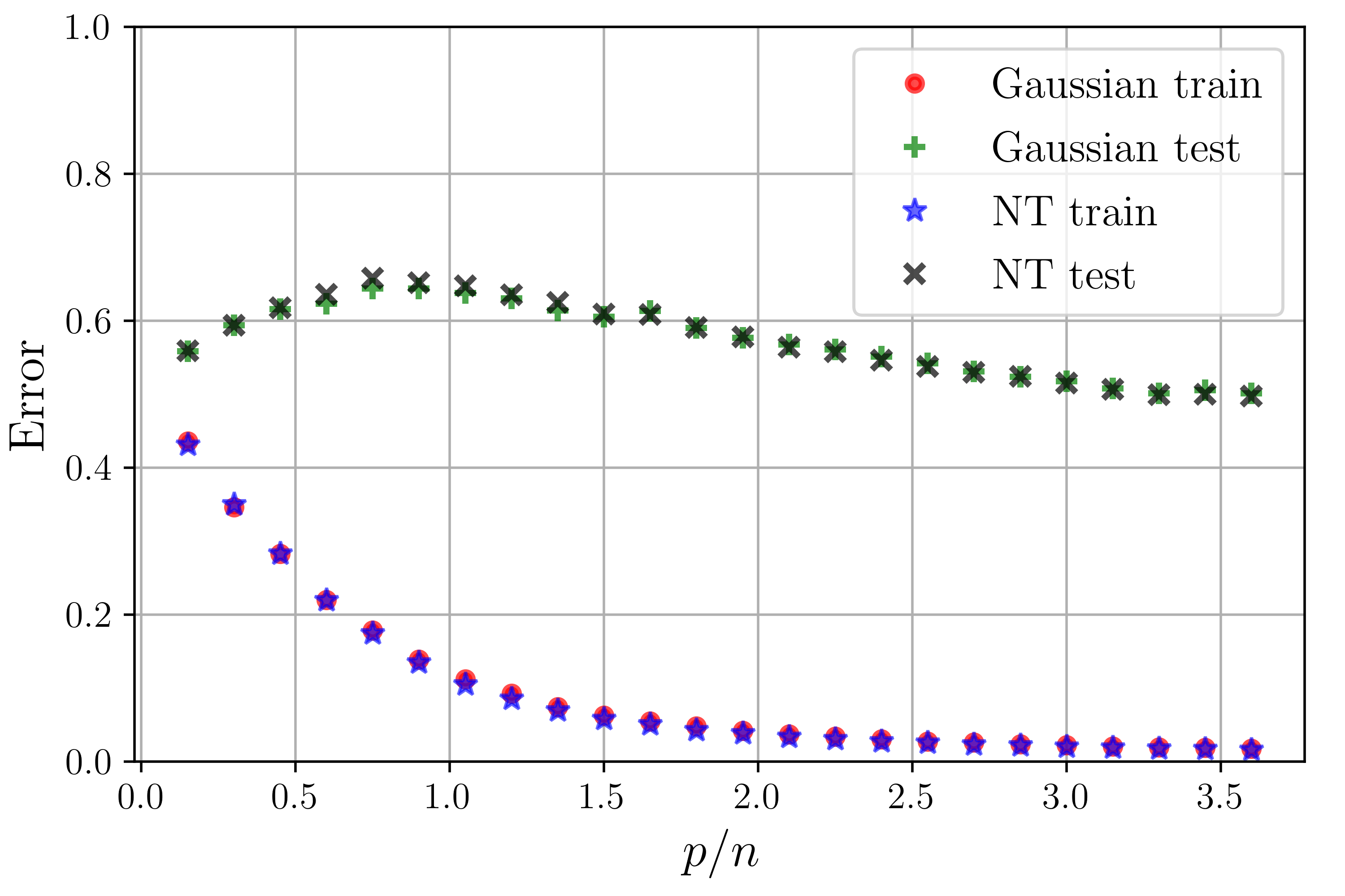
(a)

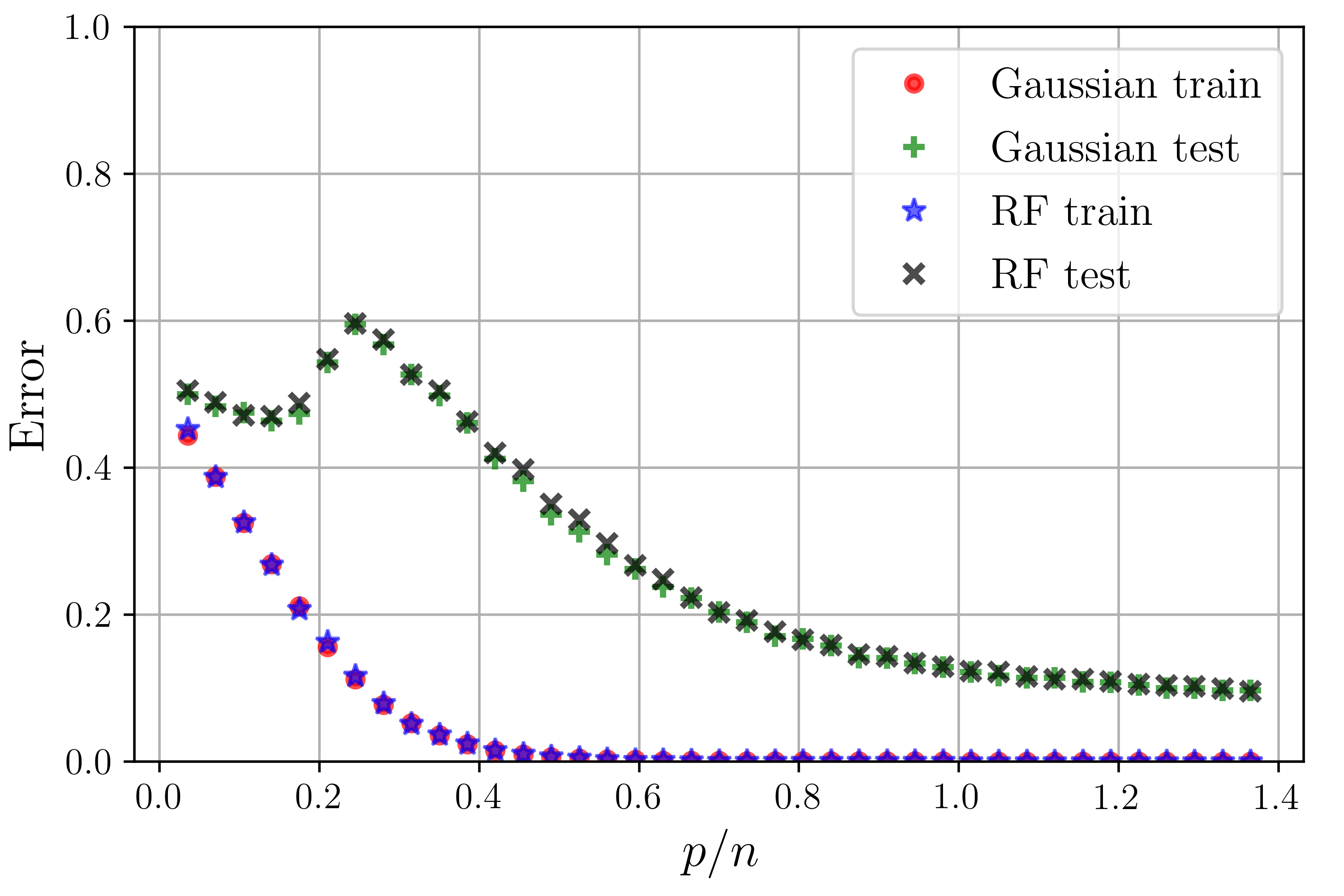
(b)

Figure 1: Universality of the training and test errors in a simulation experiment: see main text for description. In both figures, we take sample size $n=200$ and noise standard deviation $\nu=0.1$. In figure $(a)$, we take latent dimension $d=30$, regularization $\lambda=0.02$ and a neural tangent featurization map. In figure $(b)$, we take $d=100,\lambda=0.0002$ and a random features map. We vary the number of features $p$, and at each point we report the average over 100 realizations.

We follow the random matrix theory literature [Tao12] and refer to this as a universality phenomenon. When universality holds, the ERM behavior is roughly independent of the features distribution, provided their covariances are matched.

Universality is a more delicate phenomenon than concentration of the empirical risk around its expectation. Indeed, as emphasized above, it holds in the high-dimensional regime in which test error and train error do not match. Establishing universality requires understanding the dependence of the empirical risk minimizer $\widehat{\bm{\Theta}}_{n}^{\bm{X}}$ on the data ${\bm{X}},{\bm{y}}$, as opposed to just bounding its distance from a population value via concentration.

Universality for non-linear random feature models was proven for the special case of ridge regression in [HMRT19] and [MM19]. This corresponds to the ERM problem (5) whereby $\textsf{k}=1$, $\ell(u,y)=(u-y)^{2}$, and $r({\bm{\Theta}})=\lambda\|{\bm{\Theta}}\|_{2}^{2}$. At the same time, [GMKZ20, GRM⁺20] provided heuristic arguments and empirical results indicating that universality holds for other ERM problems as well.

Universality results for ERM were proven in the past for feature vectors ${\bm{x}}_{i}$ with independent entries [KM11, MN17, PH17, HS22]. Related results for randomized dimension reduction were obtained in [OT18]. The case of general vectors ${\bm{x}}_{i}$ is significantly more challenging. To the best of our knowledge, the first and only proof of universality beyond independent entries was given in the recent paper of Hu and Lu [HL20].

The result of [HL20] is limited to strongly convex ERM problems. Their proof uses a Lindeberg swapping argument, whereby the rows of ${\bm{X}}$ are replaced one-by-one by Gaussian rows with the same mean and covariance. This requires bounding at each step the resulting change in train error $\min_{{\bm{\Theta}}}\widehat{R}_{n}({\bm{\Theta}};{\bm{Z}},{\bm{y}})$, which the authors achieve by bounding the change in the minimizer. Strong convexity is crucial in this type of proof to control the change of minimizer under a perturbation of the cost.

Modern machine learning algorithms often use formulations that are either convex but not strongly convex, or non-convex, as in the example (4). Further, from a mathematical standpoint, there is no reason to believe that strong convexity should be the ‘right’ condition for universality.

In this paper, we present the following contributions:

1. Universality of training error. We prove that under suitable conditions on the features ${\bm{x}}_{i}$, the train error (the asymptotic value of $\min_{{\bm{\Theta}}}\widehat{R}_{n}({\bm{\Theta}};{\bm{X}},{\bm{y}})$) is universal for general Lipschitz losses $\ell({\bm{u}};y)$ and regularizers $r({\bm{\Theta}})$.

2. Universality of test error. We prove that, under additional regularity conditions, the test error is also universal. We emphasized that these regularity conditions concern the asymptotics of the equivalent Gaussian model. Hence, they can be checked using existing techniques.

3. Applications. We prove that our results can be applied to feature vectors ${\bm{x}}_{i}={\bm{\phi}}({\bm{z}}_{i})$ that are obtained by two interesting classes of featurization maps: random feature models (random one-layer neural networks) and neural tangent models (obtained by the first-order Taylor expansion of two-layer neural networks).

In the next section we state our main results. Then, in Section 3, we discuss our assumptions on the data distribution and prove that they are satisfied for random features and neural tangent models. In Section 4, we demonstrate via a counter-example that universality can fail to hold without this distributional assumption. Finally, in Section 5, we outline the proof of the main result. Most of the technical work is presented in the appendices.

2 Main results

2.1 Definitions and notations

We reserve the sans-serif font for parameters that are considered as fixed. We use $\left\lVert X\right\rVert_{\psi_{2}}$ and $\left\lVert f\right\rVert_{{\mbox{\tiny\rm Lip}}}$ to denote the subgaussian norm of a random variable $X$ and the Lipschitz modulus of a function $f$, respectively, and $B_{q}^{p}(r)$ to denote the $\ell_{q}$ ball of radius $r$ in $\mathbb{R}^{p}$.

We denote the feature vectors by ${\bm{x}}_{i}\in\mathbb{R}^{p}$, and the equivalent Gaussian vectors by ${\bm{g}}_{i}\in\mathbb{R}^{p}$, and introduce the matrices:

$${\bm{X}}:=({\bm{x}}_{1},\dots,{\bm{x}}_{n})^{\mathsf{T}},\quad{\bm{G}}:=({\bm{g}}_{1},\dots,{\bm{g}}_{n})^{\mathsf{T}}\,.$$

Throughout, the vectors $\{{\bm{x}}_{i}\}_{i\leq n}$ are i.i.d. and $\{{\bm{g}}_{i}\}_{i\leq n}{\stackrel{{\scriptstyle i.i.d.}}{{\sim}}}\mathcal{N}(\mu_{\bm{g}},\bm{\Sigma}_{\bm{g}})$. As mentioned above, we consider the proportional asymptotics $p,n\to\infty$ whereby, assuming without loss of generality $p:=p(n)$, we have

$$\lim_{n\to\infty}\frac{p(n)}{n}=\sgamma\in(0,\infty).$$

In fact most of our statements hold under the slightly more general assumption of $p/n\in[C^{-1},C]$

We assume that the response $y_{i}$ depends on the feature vector ${\bm{x}}_{i}$ through a low-dimensional projection ${\bm{\Theta}}^{\star{\mathsf{T}}}{\bm{x}}_{i}$, where ${\bm{\Theta}}^{\star}=({\bm{\theta}}^{\star}_{1},\dots,{\bm{\theta}}^{\star}_{\textsf{k}^{\star}})\in\mathbb{R}^{p\times\textsf{k}^{\star}}$ is a fixed matrix of parameters. Namely, we let ${\bm{\varepsilon}}:=(\varepsilon_{1},\dots,\varepsilon_{n})$ where $\{\varepsilon_{i}\}_{i\leq n}$ are i.i.d. and set:

$$y_{i}:=\eta\left({\bm{\Theta}}^{\star{\mathsf{T}}}{\bm{x}}_{i},\varepsilon_{i}\right)$$ (7)

for $\eta:\mathbb{R}^{\textsf{k}^{\star}+1}\to\mathbb{R}$. We write ${\bm{y}}({\bm{X}})$ or $y_{i}({\bm{x}}_{i})$ when we want to make the functional dependence of ${\bm{y}}$ on ${\bm{X}}$ explicit.

We denote the model parameters by ${\bm{\Theta}}=({\bm{\theta}}_{1},\dots,{\bm{\theta}}_{\textsf{k}})$, where ${\bm{\theta}}_{k}\in\mathbb{R}^{p}$ for $k\in[\textsf{k}]$, and estimate them by minimizing the regularized empirical risk of Eq. (5), subject to ${\bm{\theta}}_{k}\in{\mathcal{C}}_{p}$. Namely, we consider the problem

$$\widehat{R}^{\star}_{n}({\bm{X}},{\bm{y}}):=\inf_{{\bm{\Theta}}\in{\mathcal{C}}_{p}^{\textsf{k}}}\widehat{R}_{n}({\bm{\Theta}};{\bm{X}},{\bm{y}}),$$ (8)

for some ${\mathcal{C}}_{p}\subset\mathbb{R}^{p}$, where ${\mathcal{C}}_{p}^{\textsf{k}}:={\mathcal{C}}_{p}\times\cdots\times{\mathcal{C}}_{p}$ (k times).

2.2 Assumptions

Our assumptions are stated in terms of the positive constants R, K, k, $\textsf{k}^{\star}$, and the positive function $\textsf{K}_{r}:\mathbb{R}_{\geq 0}\to\mathbb{R}_{>0}$. Denoting by $\sOmega=(\sgamma,\textsf{R},\textsf{K},\textsf{k},\textsf{k}^{\star},\textsf{K}_{r})$ the list of these constants, all of our results will be uniform with respect to the class of problems that satisfy the assumptions at a given $\sOmega$.

The assumptions also depend on a set ${\mathcal{S}}_{p}\subseteq{\mathbb{R}}^{p\times\textsf{k}}$: this should be interpreted as the set of parameter matrices ${\bm{\Theta}}\in{\mathbb{R}}^{p\times\textsf{k}}$ such that ${\bm{\Theta}}{\bm{x}}_{1}$ is approximately Gaussian. As discussed in detail in Section 4, restricting to such a set ${\mathcal{S}}_{p}$ is unavoidable.

We will establish a general universality result under certain assumptions depending on the set ${\mathcal{S}}_{p}$, and then characterize the set ${\mathcal{S}}_{p}$ on a case-by-case basis. In Section 3 we carry out this program by explicitly determining the set ${\mathcal{S}}_{p}$ for models arising from the analysis of two-layer neural networks in the neural tangent regime.

Assumption 1 (Loss and labeling functions).

One of the following holds:

1. The loss function $\ell:\mathbb{R}^{\textsf{k}+1}\to\mathbb{R}$ is nonnegative Lipschitz with $\left\lVert\ell\right\rVert_{{\mbox{\tiny\rm Lip}}}\leq\textsf{K}$, the labels are distributed according to Eq. (7), where the labeling function $\eta:\mathbb{R}^{\textsf{k}^{\star}+1}\to\mathbb{R}$ is Lipschitz with $\left\lVert\eta\right\rVert_{{\mbox{\tiny\rm Lip}}}\leq\textsf{K}$, and the noise variables $\varepsilon_{i}$ are subgaussian, independent of ${\bm{x}}_{i}$, and satisfy $\|\varepsilon_{i}\|_{\psi_{2}}\leq\textsf{K}$ for all $i\leq n$.

2. The loss $\ell$ is nonnegative and satisfies for all ${\bm{v}},\widetilde{\bm{v}}\in\mathbb{R}^{\textsf{k}}$, $y,\widetilde{y}\in\mathbb{R}$,

   $$\left|\ell({\bm{v}},y)-\ell(\widetilde{\bm{v}},y)\right|\leq\textsf{K}\left(1+|y|\right)\left\lVert{\bm{v}}-\widetilde{\bm{v}}\right\rVert_{2},\quad\left|\ell({\bm{v}},y)-\ell({\bm{v}},\widetilde{y})\right|\leq\textsf{K}\left(1+\left\lVert{\bm{v}}\right\rVert_{2}\right)|y-\widetilde{y}|.$$

   The labels are binary: $y_{i}\in\{+1,-1\}$ with

   $$\mathbb{P}\left(y_{i}=+1|{\bm{x}}_{i}\right)=g\left({\bm{\Theta}}_{\star}^{{\mathsf{T}}}{\bm{x}}_{i}\right)\,$$ (9)

   for some $g:{\mathbb{R}}^{\textsf{k}^{\star}}\to[0,1]$ satisfying for ${\bm{v}},\widetilde{\bm{v}}\in\mathbb{R}^{\textsf{k}^{\star}}$

   $$|g({\bm{v}})-g(\widetilde{\bm{v}})|\leq\textsf{K}(1+\left\lVert{\bm{v}}\right\rVert_{2}+\left\lVert\widetilde{\bm{v}}\right\rVert_{2})\left\lVert{\bm{v}}-\widetilde{\bm{v}}\right\rVert_{2}.$$ (10)

Assumption 2 (Constraint set).

The set ${\mathcal{C}}_{p}$ appearing in the constraint in (8) is a compact subset of ${\mathcal{S}}_{p}$.

Assumption 3 (Distribution parameters).

For all $k\in[\textsf{k}^{\star}]$ and $p\in\mathbb{Z}_{>0}$ we have ${\bm{\theta}}_{k}^{\star}\in{\mathcal{S}}_{p}$.

Assumption 4 (Regularization).

The penalty function $r({\bm{\Theta}})$ is locally Lipschitz in Frobenius norm, uniformly in $p$. That is, for all $p\in\mathbb{Z}_{>0}$, $B>0$, and ${\bm{\Theta}},\widetilde{\bm{\Theta}}\in\mathbb{R}^{p\times\textsf{k}}$ satisfying $\left\lVert{\bm{\Theta}}\right\rVert_{F},\|{\widetilde{\bm{\Theta}}}\|_{F}\leq B$, we have

$$\big{|}r({\bm{\Theta}})-r(\widetilde{\bm{\Theta}})\big{|}\leq\textsf{K}_{r}(B)\big{\|}{{\bm{\Theta}}-\widetilde{\bm{\Theta}}}\big{\|}_{F}.$$

Assumption 5 (Pointwise normality).

Recall that the random vectors $\{{\bm{x}}_{i}\}_{i\leq n}$ are assumed to be i.i.d. and that $\{{\bm{g}}_{i}\}_{i\leq n}{\stackrel{{\scriptstyle i.i.d.}}{{\sim}}}\mathcal{N}({\bm{\mu}}_{\bm{g}},\bm{\Sigma}_{\bm{g}})$. We assume

$$\sup_{\{{\bm{\theta}}\in{\mathcal{S}}_{p}:\left\lVert{\bm{\theta}}\right\rVert_{2}\leq 1\}}\left\lVert{\bm{x}}^{\mathsf{T}}{\bm{\theta}}\right\rVert_{\psi_{2}}\leq\textsf{K},\quad\sup_{\{{\bm{\theta}}\in{\mathcal{S}}_{p}:\left\lVert{\bm{\theta}}\right\rVert_{2}\leq 1\}}\big{\|}{\bm{\Sigma}_{\bm{g}}^{1/2}{\bm{\theta}}}\big{\|}_{2}\leq\textsf{K},\quad\left\lVert{\bm{\mu}}_{\bm{g}}\right\rVert_{2}\leq\textsf{K}$$ (11)

Further, for any bounded Lipschitz function $\varphi:\mathbb{R}\to\mathbb{R}$,

$$\lim_{p\to\infty}\sup_{{\bm{\theta}}\in{\mathcal{S}}_{p}}\Big{|}\mathbb{E}\big{[}\varphi\big{(}{\bm{\theta}}^{\mathsf{T}}{\bm{x}}\big{)}\big{]}-\mathbb{E}\big{[}\varphi\big{(}{\bm{\theta}}^{\mathsf{T}}{\bm{g}}\big{)}\big{]}\Big{|}=0.$$ (12)

Remark 2.1.

Universality of the training error amounts to saying that $\widehat{R}^{\star}_{n}({\bm{X}},{\bm{y}}({\bm{X}}))$ is asymptotically distributed as $\widehat{R}^{\star}_{n}({\bm{G}},{\bm{y}}({\bm{G}}))$. Namely, the two risks are similarly distributed at their respective, random, minimizers $\widehat{\bm{\Theta}}_{n}^{\bm{X}}$ and $\widehat{\bm{\Theta}}_{n}^{\bm{G}}$ in ${\mathcal{C}}_{p}^{\textsf{k}}\subseteq{\mathcal{S}}_{p}^{\textsf{k}}$.

It is intuitively clear that for this to happen, their expectations must be close at a fixed, non-random point ${\bm{\Theta}}$ namely

$$0 =\lim_{n\to\infty}\big{|}\mathbb{E}\widehat{R}_{n}({\bm{\Theta}};{\bm{X}},{\bm{y}}({\bm{X}}))-\mathbb{E}\widehat{R}_{n}({\bm{\Theta}};{\bm{G}},{\bm{y}}({\bm{G}}))\big{|}$$ (13)

$$=\lim_{n\to\infty}\big{|}\mathbb{E}\,\ell({\bm{\Theta}}^{{\mathsf{T}}}{\bm{x}}_{1};\eta({\bm{\Theta}}^{\star{\mathsf{T}}}{\bm{x}}_{1};\varepsilon_{1}))-\mathbb{E}\,\ell({\bm{\Theta}}^{{\mathsf{T}}}{\bm{g}}_{1};\eta({\bm{\Theta}}^{\star{\mathsf{T}}}{\bm{g}}_{1};\varepsilon_{1}))\big{|}\,.$$

Obviously, universality of the minimum of a random function is much stronger than universality of the the function evaluated at a single point, and therefore our main results require substantial technical work.

Equation (13) amounts to saying that the distributions of ${\bm{\Theta}}^{{\mathsf{T}}}{\bm{x}}_{1}$ and ${\bm{\Theta}}^{{\mathsf{T}}}{\bm{g}}_{1}$ match when tested against a specific function (defined in terms of $\ell$ and $\eta$). Requiring this to hold for all ${\bm{\Theta}}\in{\mathcal{S}}_{p}^{\textsf{k}}$ essentially amounts to Eq. (12). In other words, we regard this assumption as roughy equivalent to assuming universality of the expected risk at a fixed point.

We will further discuss this assumption in Section 3. In particular, we will provide a counterexample showing that this or a similar assumption is necessary for universality to hold.

Remark 2.2.

The largest sequence of sets $\{{\mathcal{S}}_{p}\}$ for which Eq. (12) can hold depends on the distribution of the feature vectors ${\bm{x}}_{i}$. As illustrated by the examples of Section 3, the sets ${\mathcal{S}}_{p}$ are often determined by the condition that that no small subset of entries in ${\bm{\Theta}}$ dominates the $\ell_{2}$ norm of ${\bm{\Theta}}$.

Also note that Eq. (11) states that the projections of ${\bm{x}}$ and ${\bm{g}}$ in the direction of ${\mathcal{S}}_{p}$ are K-subgaussian, which is implied if ${\bm{x}}$ and ${\bm{g}}$ are K-subgaussian.

We additionally provide an alternative for Assumption 1 which is sufficient for our results to hold, but not as straightforward to check.

Assumption 1^′.

The nonnegative loss function $\ell$ and the labeling function $\eta$ are differentiable with locally Lipschitz gradients that satisfy

$$\left\lVert\nabla\ell({\bm{u}})\right\rVert_{2}\leq\textsf{K}\left(1+\left\lVert{\bm{u}}\right\rVert_{2}\right),\quad\left\lVert\nabla\eta({\bm{u}})\right\rVert_{2}\leq\textsf{K}\left(1+\left\lVert{\bm{u}}\right\rVert_{2}\right)$$

for all ${\bm{u}}\in\mathbb{R}^{\textsf{k}+1}$; and the noise variables $\varepsilon_{i}$ are subgaussian, independent of ${\bm{x}}_{i}$, and satisfy $\|\varepsilon_{i}\|_{\psi_{2}}\leq\textsf{K}$ for all $i\leq n$. Furthermore, for any random variables ${\bm{v}}\in\mathbb{R}^{\textsf{k}},{\bm{v}}^{\star}\in\mathbb{R}^{\textsf{k}^{\star}},V\in\mathbb{R}$ satisfying

$$\left\lVert{\bm{v}}\right\rVert_{\psi_{2}}\vee\left\lVert{\bm{v}}^{\star}\right\rVert_{\psi_{2}}\vee\left\lVert V\right\rVert_{\psi_{2}}\leq 2(\textsf{R}+1)\textsf{K}$$ (14)

and any $\beta>0$, we have

$$\mathbb{E}\left[\exp\left\{\beta\left|\ell\big{(}{\bm{v}},\eta({\bm{v}}^{\star},V)\big{)}\right|\right\}\right]\leq C(\beta,\textsf{R},\textsf{K})$$ (15)

for some $C(\beta,\textsf{R},\textsf{K})$ dependent only on $\beta,\textsf{R},\textsf{K}$.

We remark that if $\ell$ and $\eta$ satisfy Assumption 1, then it is easy to see that (15) holds.

2.3 Universality of the training error

Theorem 1.

Suppose that either Assumption 1 or Assumption 1’ holds along with assumptions 2-5. Then, for any bounded Lipschitz function $\psi:\mathbb{R}\to\mathbb{R}$,

$$\lim_{n\to\infty}\left|\mathbb{E}\left[\psi\left(\widehat{R}^{\star}_{n}\left({\bm{X}},{\bm{y}}({\bm{X}})\right)\right)\right]-\mathbb{E}\left[\psi\left(\widehat{R}^{\star}_{n}\left({\bm{G}},{\bm{y}}({\bm{G}})\right)\right)\right]\right|=0.$$ (16)

Hence, for any constant $\rho\in\mathbb{R}$ and $\delta>0$, we have

$$\lim_{n\to\infty}\mathbb{P}\left(\widehat{R}^{\star}_{n}\left({\bm{X}},{\bm{y}}({\bm{X}})\right)\geq\rho+\delta\right) \leq\lim_{n\to\infty}\mathbb{P}\left(\widehat{R}^{\star}_{n}\left({\bm{G}},{\bm{y}}({\bm{G}})\right)\geq\rho\right),\textrm{ and }$$

$$\lim_{n\to\infty}\mathbb{P}\left(\widehat{R}^{\star}_{n}\left({\bm{X}},{\bm{y}}({\bm{X}})\right)\leq\rho-\delta\right) \leq\lim_{n\to\infty}\mathbb{P}\left(\widehat{R}^{\star}_{n}\left({\bm{G}},{\bm{y}}({\bm{G}})\right)\leq\rho\right).$$ (17)

Consequently, for all $\rho\in\mathbb{R}$,

$$\widehat{R}^{\star}_{n}({\bm{X}},{\bm{y}}({\bm{X}}))\stackrel{{\scriptstyle\mathbb{P}}}{{\to}}\rho\quad\textrm{if and only if}\quad\widehat{R}^{\star}_{n}({\bm{G}},{\bm{y}}({\bm{G}}))\stackrel{{\scriptstyle\mathbb{P}}}{{\to}}\rho.$$ (18)

Remark 2.3.

Theorem 1 is the key technical result of this paper. While the training error is not as interesting as the test error, which is treated next, universality of the training error is more robust and we will build on it to establish universality of the test error.

The mathematical reason for the greater robustness of the training error is easy to understand. A small data perturbation, changing $\widehat{R}_{n}({\bm{\Theta}},{\bm{X}},{\bm{y}})$ to $\widehat{R}_{n}({\bm{\Theta}},{\bm{X}}^{\prime},{\bm{y}}^{\prime})$, changes the value of the minimum by at most $\sup_{{\bm{\Theta}}}|\widehat{R}_{n}({\bm{\Theta}},{\bm{X}},{\bm{y}})-\widehat{R}_{n}({\bm{\Theta}},{\bm{X}}^{\prime},{\bm{y}}^{\prime})|$, but can change the minimizer by a large amount. The situation is of course significantly simpler if the cost is strongly convex, since in that case the change of the minimizer is controlled as well.

Remark 2.4.

By Assumption 2, the ERM problem is subject to the constraint ${\bm{\Theta}}\in{\mathcal{C}}_{p}^{\textsf{k}}\subseteq{\mathcal{S}}_{p}$. In order to apply this theorem to unconstrained ERM problems, or to an ERM problem in which the constraint set is not a subset of ${\mathcal{S}}_{p}$, one can proceed in three steps: $(i)$ Prove that the unconstrained minimizer belongs, with high probability, to such a set ${\mathcal{C}}_{p}^{\textsf{k}}$; $(ii)$ Deduce that the unconstrained ERM problem is equivalent to the constrained one; $(iii)$ Apply Theorem 1.

Proof technique. We outline the proof of Theorem 1 in Section 5. The proof is based on an interpolation method. Namely we consider an ERM problem with feature matrix ${\bm{U}}_{t}=\sin(t){\bm{X}}+\cos(t){\bm{G}}$ that continuously interpolates between the two cases as $t$ goes from $0$ to $\pi/2$. We then bound the change in the training error (minimum empirical risk) along this path.

This approach is analogous to the Lindeberg method [Lin22, Cha06], which was used in the context of statistical learning in [KM11] and subsequently in [MN17, OT18, HL20]. A direct application of the Lindeberg procedure would require to swap an entire row of ${\bm{X}}$ with the corresponding row of ${\bm{G}}$ and bound the effect on the minimum empirical risk (we cannot replace one entry at a time since these are dependent). We find the use of a continuous path more effective.

In [HL20], the effect of a swapping step is controlled by first bounding the change in the minimizer $\widehat{\bm{\Theta}}$. This is achieved by assuming strong convexity of the empirical risk. The bound in the change of the minimizer immediately implies a bound in the change of the minimum value.

In the non-convex setting, we face the challenge of bounding the change of the minimum without bounding the change of the minimizer. We achieve this by using a differentiable approximation of the minimum. Even after this sequence of approximations, unlike in other universality proofs, the expectation one needs to bound is not obviously small. The key technical innovation is a polynomial approximation method which we believe can be of more general applicability.

2.4 Universality of the test error

Let us define the test error

$$R_{n}^{\bm{x}}({\bm{\Theta}}):=\mathbb{E}\Big{[}\ell\big{(}{\bm{\Theta}}^{\mathsf{T}}{\bm{x}};\eta({\bm{\Theta}}^{\star{\mathsf{T}}}{\bm{x}},\varepsilon)\big{)}\Big{]},\quad R_{n}^{\bm{g}}({\bm{\Theta}}):=\mathbb{E}\Big{[}\ell\big{(}{\bm{\Theta}}^{\mathsf{T}}{\bm{g}};\eta({\bm{\Theta}}^{\star{\mathsf{T}}}{\bm{g}},\varepsilon)\big{)}\Big{]}.$$

The first expectation is with respect to independent random variables ${\bm{x}}\sim\mathbb{P}_{{\bm{x}}}$ and $\varepsilon\sim\mathbb{P}_{\varepsilon}$, and the second with respect to independent ${\bm{g}}\sim{\mathcal{N}}({\bm{\mu}}_{\bm{g}},\bm{\Sigma}_{{\bm{g}}})$ and $\varepsilon\sim\mathbb{P}_{\varepsilon}$. As discussed above, it is easy to see that, under Assumption 5, $\lim_{n\to\infty}|R_{n}^{\bm{x}}({\bm{\Theta}})-R_{n}^{\bm{g}}({\bm{\Theta}})|=0$ at a fixed ${\bm{\Theta}}$. Here however we are interested in comparing the two at near minimizers of the respective ERM problems.

We will state two theorems that provide sufficient conditions for universality of the test error. The first of these theorems concerns a scenario in which near interpolators (models achieving very small training error) exist. We are interested in this scenario because of its relevance to deep learning [BMR21], and because it is very different from the strongly convex one.

It is useful to denote the set of near empirical risk minimizers:

$${\textrm{ERM}}_{t}({\bm{X}}):=\big{\{}{\bm{\Theta}}\in{\mathcal{C}}_{p}^{\textsf{k}}\mbox{ s.t. }\widehat{R}_{n}({\bm{\Theta}};{\bm{X}},{\bm{y}}({\bm{X}}))\leq t\big{\}}\,.$$ (19)

Theorem 2.

Assume $\lim_{n\to\infty}\mathbb{P}({\textrm{ERM}}_{0}({\bm{G}})\neq\emptyset)=1$. Then under Assumptions 1-5, for all $\delta>0,\alpha>0$ and $\rho\in\mathbb{R}$ we have

$$\lim_{n\to\infty}\mathbb{P}\Big{(}\min_{{\bm{\Theta}}\in{{\textrm{ERM}}}_{\alpha}({\bm{X}})}R_{n}^{\bm{x}}({\bm{\Theta}})\geq\rho+\delta\Big{)} \leq\lim_{n\to\infty}\mathbb{P}\Big{(}\min_{{\bm{\Theta}}\in{\textrm{ERM}}_{0}({\bm{G}})}R_{n}^{\bm{g}}({\bm{\Theta}})>\rho\Big{)},\textrm{ and }$$

$$\lim_{t\to 0}\lim_{n\to\infty}\mathbb{P}\Big{(}\min_{{\bm{\Theta}}\in{\textrm{ERM}}_{t}({\bm{X}})}R_{n}^{\bm{x}}({\bm{\Theta}})\leq\rho-\delta\Big{)} \leq\lim_{n\to\infty}\mathbb{P}\Big{(}\min_{{\bm{\Theta}}\in{\textrm{ERM}}_{\alpha}({\bm{G}})}R_{n}^{\bm{g}}({\bm{\Theta}})\leq\rho\Big{)}.$$

In other words, the minimum test error over all near-interpolators is universal (provided it does not change discontinuously with the accuracy of ‘near interpolation’). The same theorem holds (with identical proof) for the maximum test error over near interpolators, and if the level $0$ is replaced with any deterministic constant.

Corollary 1.

Assume $\lim_{n\to\infty}\mathbb{P}({\textrm{ERM}}_{0}({\bm{G}})\neq\emptyset)=1$. and that Assumptions 1-5 hold. Further assume that the following limits exist for $t\in[0,t_{0}]$ with $t_{0}$ a small enough constant:

$$\operatorname*{p-lim}_{n\to\infty}\min_{{\bm{\Theta}}\in{\textrm{ERM}}_{t}({\bm{G}})}R_{n}^{\bm{g}}({\bm{\Theta}}) =\rho(t)\,,$$ (20)

$$\lim_{t\to 0}\rho(t) =\rho(0)\,.$$ (21)

(In the first line $\operatorname*{p-lim}$ denotes limit in probability.)

Then we have

$$\lim_{t\to 0}\operatorname*{p-lim}_{n\to\infty}\min_{{\bm{\Theta}}\in{\textrm{ERM}}_{t}({\bm{X}})}R_{n}^{\bm{x}}({\bm{\Theta}}) =\rho(0)\,.$$ (22)

The next theorem provides alternative sufficient conditions that guarantee the universality of the test error. We emphasize that these are conditions on the Gaussian features only and it is therefore possible to check them on concrete models using existing techniques.

Theorem 3.

Suppose one of the following holds:

1. The loss $\ell(\;\cdot\;;y)$ is convex for fixed $y$, the regularizer $r$ is $\smu$-strongly convex for some fixed constant $\smu>0$ and ${\mathcal{C}}_{p}\subseteq{\mathcal{S}}_{p}$ is given by ${\mathcal{C}}_{p}=\{{\bm{\theta}}\in\mathbb{R}^{p}:h({\bm{\theta}})\leq L\}$ for some convex $h$ and $L\in\mathbb{R}$. Furthermore, we have for some $\rho,\widetilde{\rho}\in\mathbb{R}$

   $$\widehat{R}_{n}^{\star}\left({\bm{G}},{\bm{y}}({\bm{G}})\right)\stackrel{{\scriptstyle\mathbb{P}}}{{\to}}\rho,\quad R_{n}^{\bm{g}}\left(\widehat{\bm{\Theta}}_{n}^{\bm{G}}\right)\stackrel{{\scriptstyle\mathbb{P}}}{{\to}}\widetilde{\rho}\,;$$

2. For some $\rho,\widetilde{\rho}\in\mathbb{R}$, let ${\mathcal{U}}_{p}(\widetilde{\rho},\alpha):=\{{\bm{\Theta}}\in{\mathcal{C}}_{p}^{\textsf{k}}:\;|R_{n}^{\bm{g}}({\bm{\Theta}})-\widetilde{\rho}|\geq\alpha\}$. We have $\widehat{R}_{n}^{\star}({\bm{G}},{\bm{y}}({\bm{G}}))\stackrel{{\scriptstyle\mathbb{P}}}{{\to}}\rho$, and for all $\alpha>0$, there exists $\delta>0$ so that

   $$\lim_{n\to\infty}\mathbb{P}\Big{(}\min_{{\bm{\Theta}}\in{\mathcal{U}}_{p}(\widetilde{\rho},\alpha)}|\widehat{R}_{n}({\bm{\Theta}};{\bm{G}},{\bm{y}}({\bm{G}}))-\widehat{R}_{n}^{\star}({\bm{G}},{\bm{y}}({\bm{G}}))|\geq\delta\Big{)}=1;$$

3. there exists a function $\rho(s)$ differentiable at $s=0$ such that for all $s$ in a neighborhood of $0$,

   $$\min_{{\bm{\Theta}}\in{\mathcal{C}}_{p}^{\textsf{k}}}\Big{\{}\widehat{R}_{n}({\bm{\Theta}};{\bm{G}},{\bm{y}}({\bm{G}}))+sR_{n}^{\bm{g}}({\bm{\Theta}})\Big{\}}\stackrel{{\scriptstyle\mathbb{P}}}{{\to}}\rho(s).$$ (23)

Then, under Assumptions 1-5,

$$\left|R_{n}^{\bm{x}}\left(\widehat{\bm{\Theta}}_{n}^{\bm{X}}\right)-R_{n}^{\bm{g}}\left(\widehat{\bm{\Theta}}_{n}^{\bm{G}}\right)\right|\stackrel{{\scriptstyle\mathbb{P}}}{{\to}}0$$

for any minimizers $\widehat{\bm{\Theta}}_{n}^{\bm{X}},\widehat{\bm{\Theta}}_{n}^{\bm{G}}$ of $\widehat{R}_{n}({\bm{\Theta}};{\bm{X}},{\bm{y}}({\bm{X}}))$, $\widehat{R}_{n}({\bm{\Theta}};{\bm{G}},{\bm{y}}({\bm{G}}))$, respectively.

Proof technique. The proofs of Theorems 2 and 3 are given in Appendix B and C. The basic technique can be gleaned from condition (23). We perturb the train error by a term proportional to the test error (this is only a proof device, not an actual algorithm). The test error can be related to the derivative with respect to $s$ of the resulting minimum value. The minimum value is universal by our results in the previous section. The technical challenge is therefore to control its derivative.

3 Checking pointwise normality

In this section we study some concrete examples for the distribution of the feature vectors ${\bm{x}}_{i}$. In each case, we characterize the set of parameter vectors ${\mathcal{S}}_{p}$ for which the pointwise normality condition of Eq. (12) holds. For simplicity of exposition, we use $\textsf{k}=\textsf{k}^{\star}=1$ throughout this section.

We first consider examples of featurization maps from the deep learning literature. Section 3.1 analyzes the featurization map that is obtained by linearizing a two-layer neural network around a random initialization. This is also known as the ‘neural tangent model.’ We establish asymptotic equivalence (in distributional sense) of ERM under the neural tangent model, to ERM under the Gaussian model with matching covariance structure. Comparable universality results were not known in this model, even in the case of convex losses. Indeed, checking the pointwise normality condition of Eq. (12) is challenging in this case.

Next, in Section 3.2, we consider the featurization map that is obtained by applying a one-layer network with random weights. This is equivalent to the ‘random features’ model of [RR07]. Pointwise normality (along the lines of Eq. (12)) and universality of the expected risk at a fixed ${\bm{\Theta}}$ for this model was first shown in [GRM⁺20]. Universality of test and train error for ridge regression was established in [MM19], while [HL20] proved universality of the ERM for strongly convex losses. Finally, [LGC⁺21] presented empirical evidence and conjectured that universality holds for a wide class of such featurization maps and loss functions.

In the setting of Section 3.2, our main contribution is the generalization of the results of [HL20] to non-convex losses.

Finally, in Section 3.3, we consider the case in which $\bm{\Sigma}^{-1/2}{\bm{x}}_{i}$ has i.i.d. entries: this is a standard model in random matrix theory. This data distribution was studied in the past mostly for convex or strongly convex losses  [MN17, PH17, OT18]. The only exception is provided by [KM11] which studies certain non-convex losses when $\bm{\Sigma}={\bm{I}}$.

As we will see, the set ${\mathcal{S}}_{p}$ typically excludes parameters ${\bm{\Theta}}$ that are too aligned with an element of the canonical basis. In other words, the parameters ${\bm{\Theta}}$ needs to be ‘incoherent’ with respect to the canonical basis.

In specific applications, if the constraint set ${\mathcal{C}}_{p}$ is not a subset of ${\mathcal{S}}_{p}$, in order to apply our general theorems, it will be necessary to prove that a minimizer actually belongs to ${\mathcal{S}}_{p}$. In general, this will require a case-by-case analysis. However, Section 3.4 shows that a minimizer satisfies this condition for a broad class of overparametrized models. In these cases, no further analysis is required.

3.1 Two layer (finite width) neural tangent model

Consider a two layer neural network with $m$ hidden neurons and fixed second layer weights $f({\bm{z}};{\bm{u}}):=\sum_{i=1}^{m}a_{i}\sigma(\langle{\bm{u}}_{i},{\bm{z}}\rangle)$, with input ${\bm{z}}\in\mathbb{R}^{d}$. Under neural tangent (a.k.a. lazy) training conditions, such a network is well approximated by a linear model with respect to the features

$${\bm{\phi}}_{\textrm{NT}}({\bm{z}}):=\left(\sigma^{\prime}({\bm{w}}_{1}^{\mathsf{T}}{\bm{z}}){\bm{z}}^{\mathsf{T}},\dots,\sigma^{\prime}({\bm{w}}_{m}^{\mathsf{T}}{\bm{z}}){\bm{z}}^{\mathsf{T}}\right)^{\mathsf{T}}\in\mathbb{R}^{p}\,,$$ (24)

where ${\bm{w}}_{i}$ are the first layer weights at initializations ${\bm{u}}_{i}^{0}={\bm{w}}_{i}$, and $p=md$. As in the rest of the paper, we assume to be given training samples $\{(y_{i},{\bm{z}}_{i})\}_{i\leq n}$ and to compute feature vectors ${\bm{x}}_{i}={\bm{\phi}}_{\textrm{NT}}({\bm{z}}_{i})$.

Here we are not concerned with the connection between the original neural network and its neural tangent model, for which we refer to the literature [JGH18, DLL⁺19, LXS⁺19, BMR21, MZ20]. We will instead focus on the neural tangent model, and show that it can be approximated by an equivalent Gaussian model. Let us emphasize once more that –despite the neural tangent approximation– the loss function which we assume for the neural tangent model is not necessarily convex.

We assume a simple covariates distribution: $\{{\bm{z}}_{i}\}_{i\leq n}{\stackrel{{\scriptstyle i.i.d.}}{{\sim}}}\mathcal{N}(0,{\bm{I}}_{d})$. Further we assume a standard network initialization: $\{{\bm{w}}_{j}\}_{j\leq m}{\stackrel{{\scriptstyle i.i.d.}}{{\sim}}}\textsf{Unif}\left(\mathbb{S}^{d-1}(1)\right)$, i.e., ${\bm{w}}_{j}$ are uniformly distributed on the sphere of radius $1$ in $\mathbb{R}^{d}$. Notice that: $(i)$ The weights ${\bm{w}}_{j}$ are fixed and do not change from sample to sample; $(ii)$ Although the covariates ${\bm{z}}_{i}$ have a simple distribution, the vectors ${\bm{x}}_{i}$ are highly non-trivial and have dependent entries (in fact they lie on a $m$-dimensional nonlinear manifold in $\mathbb{R}^{p}$, with $p\gg m$).

We assume the activation function $\sigma$ to be four times differentiable with bounded derivatives and to satisfy $\mathbb{E}[\sigma^{\prime}(G)]=0$, $\mathbb{E}[G\sigma^{\prime}(G)]=0$, for $G\sim\mathcal{N}(0,1)$. These conditions yield some mathematical simplifications and we defer relaxing them to future work. Further, we focus on $m=m(n),d=d(n)\in\mathbb{Z}_{>0}$, and $\lim_{n\to\infty}m(n)/d(n)=\widetilde{\sgamma}$ for some fixed $\widetilde{\sgamma}\in(0,\infty)$. In particular, $m,d=\Theta(p^{1/2})$, $n=\Theta(p)$.

For ${\bm{\theta}}=({\bm{\theta}}_{{(1)}}^{\mathsf{T}},\dots,{\bm{\theta}}_{(m)}^{\mathsf{T}})^{\mathsf{T}}\in\mathbb{R}^{p}$, where ${\bm{\theta}}_{{(j)}}\in\mathbb{R}^{d}$ for $j\in[m]$, let ${\bm{T}}_{\bm{\theta}}\in\mathbb{R}^{d\times m}$ be the matrix ${\bm{T}}_{\bm{\theta}}=\left({\bm{\theta}}_{(1)},\dots,{\bm{\theta}}_{(m)}\right)$, so that ${\bm{\theta}}^{\mathsf{T}}{\bm{x}}={\bm{z}}^{\mathsf{T}}{\bm{T}}_{\bm{\theta}}\sigma^{\prime}({\bm{W}}^{\mathsf{T}}{\bm{z}})$, where ${\bm{W}}=({\bm{w}}_{1},\dots,{\bm{w}}_{m}$) and $\sigma^{\prime}:\mathbb{R}\to\mathbb{R}$ is applied entrywise. We define, for $p\in\mathbb{Z}_{>0}$,

$${\mathcal{S}}_{p}:=\left\{{\bm{\theta}}\in\mathbb{R}^{p}:\left\lVert{\bm{T}}_{\bm{\theta}}\right\rVert_{\mathrm{op}}\leq\frac{\textsf{R}}{\sqrt{d}}\right\}.$$ (25)

We have the following universality result for the neural tangent model (24).

Theorem 4.

Let ${\bm{x}}_{i}={\bm{\phi}}_{\textrm{NT}}({\bm{z}}_{i})$ as per Eq. (24) with $\{{\bm{z}}_{i}\}_{i\leq n}\stackrel{{\scriptstyle\textrm{i.i.d.}}}{{\sim}}\mathcal{N}(0,{\bm{I}}_{d})$, and ${\mathcal{S}}_{p}$ be as defined in (25). Further, let $(\ell,{\bm{y}}),{\mathcal{C}}_{p},{\bm{\theta}}^{\star}$ and $r$ satisfy assumptions 1, 2, 3 and 4 respectively, and ${\bm{g}}_{i}|{\bm{W}}{\stackrel{{\scriptstyle i.i.d.}}{{\sim}}}\mathcal{N}(0,\bm{\Sigma}_{\bm{W}})$ for $\bm{\Sigma}_{\bm{W}}:=\mathbb{E}\left[{\bm{x}}{\bm{x}}^{\mathsf{T}}|{\bm{W}}\right]$. Then the following hold:

1. For any bounded Lipschitz function $\psi:\mathbb{R}\to\mathbb{R}$, Eq. (16) holds. In particular, as a consequence,

   $$\widehat{R}^{\star}_{n}({\bm{X}},{\bm{y}}({\bm{X}}))\stackrel{{\scriptstyle\mathbb{P}}}{{\to}}\rho\quad\textrm{if and only if}\quad\widehat{R}^{\star}_{n}({\bm{G}},{\bm{y}}({\bm{G}}))\stackrel{{\scriptstyle\mathbb{P}}}{{\to}}\rho.$$ (26)

2. Under the additional conditions of Theorem 2, Corollary 1 or Theorem 3, the universality results for the test error stated there hold.

Remark 3.1.

Theorem 4 does not hold if we relax the set ${\mathcal{S}}_{p}$ to ${\mathcal{S}}_{p}:=B_{2}^{p}(\textsf{R})$. Indeed, for ${\bm{T}}_{\bm{\theta}}=\textsf{R}/\sqrt{d}\left(\mathbf{1}_{d},0,\dots,0\right)$, the random variable ${\bm{\theta}}^{\mathsf{T}}{\bm{x}}={\bm{z}}^{\mathsf{T}}{\bm{T}}_{\bm{\theta}}\sigma^{\prime}({\bm{W}}^{\mathsf{T}}{\bm{z}})$ is not asymptotically Gaussian. Clearly, this choice of ${\bm{\theta}}$ is not in the set defined in (25).

Proof technique. We prove Theorem 4 in Appendix E by using Theorem 1. The key technical challenge is to establish that Assumption (5) for the distribution of the feature vectors ${\bm{x}}_{i}={\bm{\phi}}_{\textrm{NT}}({\bm{z}}_{i})$, cf. Eq. (24). We Stein’s method as done in [HL20] for the random features model. However, treating the neural tangent features of Eq. (24) requires extra care due to the more complex covariance structure.

3.2 Random features

Consider a two layer network with $p$ hidden neurons and fixed first layer weights $f({\bm{z}};{\bm{a}}):=\sum_{i=1}^{p}a_{i}\sigma(\langle{\bm{w}}_{i},{\bm{z}}\rangle)$, where ${\bm{z}}\in\mathbb{R}^{d}$. This is a linear model with respect to the features

$${\bm{\phi}}_{\textrm{RF}}({\bm{z}}):=\left(\sigma\left({\bm{w}}_{1}^{\mathsf{T}}{\bm{z}}\right),\dots,\sigma\left({\bm{w}}_{p}^{\mathsf{T}}{\bm{z}}\right)\right)^{\mathsf{T}}.$$ (27)

As before, we consider $\{{\bm{z}}_{i}\}_{i\leq n}\stackrel{{\scriptstyle\textrm{i.i.d.}}}{{\sim}}\mathcal{N}(0,{\bm{I}}_{d})$ and ${\bm{x}}_{i}={\bm{\phi}}_{\textrm{RF}}({\bm{z}}_{i})$. Further we assume the first-layer weights to be given by $\{{\bm{w}}_{j}\}_{j\leq m}\stackrel{{\scriptstyle\textrm{i.i.d.}}}{{\sim}}\textsf{Unif}\left(\mathbb{S}^{d-1}(1)\right)$.

The activation function $\sigma$ is now assumed to be three times continuously differentiable with bounded derivatives, with $\mathbb{E}\sigma(G)=0$ for $G\sim\mathcal{N}(0,1)$. (These are slightly weaker conditions than in the previous section.) We consider $d=d(n)\in\mathbb{Z}_{>0}$ such that, for some fixed $\widetilde{\sgamma}\in(0,\infty)$, $\lim_{n\to\infty}d(n)/p(n)=\widetilde{\sgamma}$. Finally, fix $\alpha>0$ and define for $p\in\mathbb{Z}_{>0}$

$${\mathcal{S}}_{p}:=\big{\{}{\bm{\theta}}\in\mathbb{R}^{p}:\;\|{\bm{\theta}}\|_{\infty}\leq\textsf{R}p^{-\alpha}\,,\|{\bm{\theta}}\|_{2}\leq\textsf{R}\big{\}}\,.$$ (28)

Let ${\bm{W}}$ be the matrix whose columns are the weights ${\bm{w}}_{j}$. We have the following corollary of Theorem 1.

Corollary 2.

Let ${\bm{x}}_{i}={\bm{\phi}}_{\textrm{RF}}({\bm{z}}_{i})$ as per Eq. (27) with $\{{\bm{z}}_{i}\}_{i\leq n}\stackrel{{\scriptstyle\textrm{i.i.d.}}}{{\sim}}\mathcal{N}(0,{\bm{I}}_{d})$, and ${\mathcal{S}}_{p}$ be as defined in (28). Further, let $(\ell,{\bm{y}}),{\mathcal{C}}_{p},{\bm{\theta}}^{\star}$ and $r$ satisfy assumptions 1, 2, 3 and 4 respectively, and ${\bm{g}}_{i}|{\bm{W}}{\stackrel{{\scriptstyle i.i.d.}}{{\sim}}}\mathcal{N}(0,\bm{\Sigma}_{\bm{W}})$ for $\bm{\Sigma}_{\bm{W}}:=\mathbb{E}\left[{\bm{x}}{\bm{x}}^{\mathsf{T}}|{\bm{W}}\right]$. Then for any bounded Lipschitz function $\psi:\mathbb{R}\to\mathbb{R}$, Eq. (16) holds along with its consequences: Eq. (17) and Eq. (18).

In Appendix F, we derive this corollary as a consequence of Theorem 1. To do so, we use a result established by [HL20] implying that the feature vectors ${\bm{x}}_{i}$ satisfy Assumption 5, for every ${\bm{W}}$ in a high probability set.

3.3 Linear functions of vectors with independent entries

Consider feature vectors ${\bm{x}}_{i}=\bm{\Sigma}^{1/2}\overline{\bm{x}}_{i}\in\mathbb{R}^{p}$, where the vectors $\overline{\bm{x}}_{i}$ have $p$ i.i.d subgaussian entries of subgaussian norm bounded by K and unit variance. We assume $\|\bm{\Sigma}\|_{\mathrm{op}}\leq\textsf{K}$. Fix any deterministic sequence $\alpha_{p}$ such that $\lim_{p\to\infty}\alpha_{p}=0$. An application of the Lindeberg central limit theorem (CLT) shows that Eq. (12) of Assumption 5 holds for

$${\mathcal{S}}_{p}:=\big{\{}{\bm{\theta}}\in\mathbb{R}^{p}:\;\|\bm{\Sigma}^{1/2}{\bm{\theta}}\|_{\infty}\leq\alpha_{p}\,,\|{\bm{\theta}}\|_{2}\leq\textsf{R}\big{\}}\,.$$ (29)

We have therefore the following corollary of Theorem 1.

Corollary 3.

Let ${\bm{x}}_{i}=\bm{\Sigma}^{1/2}\overline{\bm{x}}_{i}\in\mathbb{R}^{p}$ where $\overline{\bm{x}}_{i}$ has i.i.d. subgaussian entries with unit variance, and ${\mathcal{S}}_{p}$ be as defined in (29). Furthermore, let $(\ell,{\bm{y}}),{\mathcal{C}}_{p},{\bm{\theta}}^{\star}$ and $r$ satisfy assumptions 1, 2, 3 and 4 respectively. Let ${\bm{g}}_{i}\sim\mathcal{N}(0,\bm{\Sigma})$. Then for any bounded Lipschitz function $\psi:\mathbb{R}\to\mathbb{R}$, Eq. (16) holds along with its consequences: Eq. (17) and Eq. (18).

3.4 Controlling a minimizer in the overparametrized setting

The general universality results of Theorem 1 to Theorem 3 are stated for the ERM problem of Eq. (8), where we constrain ${\bm{\Theta}}\in{\mathcal{C}}_{p}^{\textsf{k}}\subseteq{\mathcal{S}}_{p}$, with ${\mathcal{S}}_{p}$ satisfying Assumption 5. As discussed in Remark 2.4, these theorems can be applied to unconstrained ERM problems, or to ERM problems in which the constraint set is not a subset of ${\mathcal{S}}_{p}$, by separately proving that the minimizer belongs, with high probability, to a suitable compact set ${\mathcal{C}}_{p}^{\textsf{k}}\subseteq{\mathcal{S}}_{p}$.

Proving the last property will require, in general, a case-by-case analysis. Here we limit ourselves to stating a general result in the overparametrized setting. In words, this result implies that, if there exists a global empirical risk minimizer with controlled $\ell_{2}$ norm (a condition that is relatively easy to check), then there exists also an empirical risk minimizer with controlled $\ell_{\infty}$ norm. In what follows, we continue to work under the assumption $p/n\to\sgamma\in(0,\infty)$.

Theorem 5.

Assume $p/n\geq(1+\delta)$ for some $\delta>0$, $\bm{\Sigma}^{-1/2}{\bm{x}}_{i}$ have i.i.d., mean $0$, unit variance and subgaussian entries. Further assume that there exist constants $k,K>0$ such that

$$\left\lVert\bm{\Sigma}^{-1/2}\right\rVert_{\infty\to\infty}:=\max_{i\leq p}\|(\bm{\Sigma}^{-1/2})_{i,\cdot}\|_{1}\leq K,\quad\quad k\leq\sigma_{\min}(\bm{\Sigma}^{-1/2})\leq\sigma_{\max}(\bm{\Sigma}^{-1/2})\leq K$$

and that

$$\lim_{n\to\infty}\mathbb{P}\left(\exists\widehat{\bm{\theta}}_{n}\in\operatorname*{arg\,min}_{\theta\in\mathbb{R}^{p}}\frac{1}{n}\sum_{i=1}^{n}\ell({\bm{\theta}}^{\mathsf{T}}{\bm{x}}_{i},y_{i}):\left\lVert\widehat{\bm{\theta}}_{n}\right\rVert_{2}\leq K\right)=1.$$ (30)

Then for any $\alpha<1/8$, there exists $C>0$ depending only on $\sOmega$ such that

$$\lim_{n\to\infty}\mathbb{P}\left(\exists\widehat{\bm{u}}_{n}\in\operatorname*{arg\,min}_{{\bm{\theta}}\in\mathbb{R}^{p}}\frac{1}{n}\sum_{i=1}^{n}\ell({\bm{\theta}}^{\mathsf{T}}{\bm{x}}_{i},y_{i}):\left\lVert\widehat{\bm{u}}_{n}\right\rVert_{2}\leq(C+1)K,\left\lVert\widehat{\bm{u}}_{n}\right\rVert_{\infty}\leq Kp^{-\alpha}\right)=1.$$

That is, condition (12) of Assumption 5 holds in this case. In particular, under Assumptions 1 to 4 and the subgaussian condition of Eq. (11), we have

$$\widehat{R}^{\star}_{n}({\bm{X}},{\bm{y}}({\bm{X}}))\stackrel{{\scriptstyle\mathbb{P}}}{{\to}}0\quad\textrm{if and only if}\quad\widehat{R}^{\star}_{n}({\bm{G}},{\bm{y}}({\bm{G}}))\stackrel{{\scriptstyle\mathbb{P}}}{{\to}}0,$$ (31)

where $\widehat{R}_{n}^{\star}$ is the optimum of the unconstrained ERM problem.

The proof of this result is deferred to Appendix D.

4 Necessity of pointwise normality

Let us now give a counterexample demonstrating that universality does not hold for general ERM problems, unless we restrict the optimization to subsets of ${\mathcal{S}}_{p}$ where the latter satisfies the pointwise normality condition (12).

For $i\in[n]$, let ${\bm{x}}_{i}\sim\textrm{Unif}(\{+1,-1\}^{p})$. in other words, each coordinate $x_{ij}$ is uniformly random in $\{+1,-1\}$. Consider the set ${\mathcal{S}}_{p}:=\{{\bm{\theta}}\in\mathbb{R}^{p}:\left\lVert{\bm{\theta}}\right\rVert_{2}\leq 1\}$.

The pointwise normality condition (12) is not satisfied for this distribution of the feature vectors ${\bm{x}}_{i}$ and this choice of ${\mathcal{S}}_{p}$. Indeed ${\bm{e}}_{1}=(1,0,\dots,0)^{{\mathsf{T}}}\in{\mathcal{S}}_{p}$. However ${\bm{e}}_{1}^{\mathsf{T}}{\bm{x}}\sim\textrm{Unif}(\{+1,-1\})$, while under the Gaussian model with the same covariance —namely, for ${\bm{g}}\sim\mathcal{N}(0,{\bm{I}}_{p})$— we have ${\bm{e}}_{1}^{\mathsf{T}}{\bm{g}}\sim\mathcal{N}(0,1)$, for all $p$. In other words, Assumption 5 does not hold in this case.

We next construct an ERM problem whose minimum value under this features distribution is different from the value under the Gaussian model. Consider the non-negative, Lipschitz continuous loss function

$$\ell(t):=\begin{cases}\big{|}1-|t|\big{|}&|t|\leq 2\\ 1&|t|>2\,.\end{cases}$$

We then have the following minima of the two empirical risk problems:

$$\widehat{R}_{n}^{\star}({\bm{X}}):=\min_{\left\lVert{\bm{\theta}}\right\rVert_{2}\leq 1}\frac{1}{n}\sum_{i=1}^{n}\ell({\bm{\theta}}^{\mathsf{T}}{\bm{x}}_{i})\,,\;\;\;\;\;\;\;\widehat{R}_{n}^{\star}({\bm{G}}):=\min_{\left\lVert{\bm{\theta}}\right\rVert_{2}\leq 1}\frac{1}{n}\sum_{i=1}^{n}\ell({\bm{\theta}}^{\mathsf{T}}{\bm{g}}_{i})\,.$$ (32)

In the non-Gaussian case, we clearly have $\widehat{R}_{n}^{\star}({\bm{X}})=0$ for all $n$, since $\widehat{R}_{n}^{\star}({\bm{X}})\geq 0$ by construction, while $\widehat{R}_{n}^{\star}({\bm{X}})\leq 0$ follows by evaluating the cost at $\widehat{\bm{\theta}}_{n}^{\bm{X}}={\bm{e}}_{1}$. Hence, ${\bm{e}}_{1}$ will be a minimizer which achieves a training loss of $0$ for all $n$. However, in the Gaussian model (defined by ${\bm{g}}_{i}\sim\mathcal{N}(0,{\bm{I}}_{p})$), there exist $c>0$, $\sgamma_{0}>0$ such that if $\sgamma\geq\sgamma_{0}$,

$$\lim_{n\to\infty}\mathbb{P}\left(\min_{\left\lVert{\bm{\theta}}\right\rVert_{2}\leq 1}\frac{1}{n}\sum_{i=1}^{n}\ell({\bm{\theta}}^{\mathsf{T}}{\bm{g}}_{i})\geq c\right)=1\,.$$ (33)

This can shown by a uniform convergence argument as we detail in Appendix G.1.

We finally notice that if we instead define ${\mathcal{S}}_{p}:=\{{\bm{\theta}}\in{\mathbb{R}}^{p}:\|{\bm{\theta}}\|_{2}\leq 1,\;\|{\bm{\theta}}\|_{\infty}\leq\alpha_{p}\}$ for some deterministic $\alpha_{p}$ such that $\alpha_{p}\to 0$ as $p\to\infty$ (see Eq. (29)), then condition (12) holds. Hence the universality of the minimum follows in this case from Corollary 3.

5 Proof outline for Theorem 1

We redefine the vector $\sOmega$ from our assumptions to include $\smu$ and $\widetilde{\sgamma}$: $\sOmega:=\left(\textsf{k},\textsf{k}^{\star},\sgamma,\textsf{R},\textsf{K},\textsf{K}_{r}(\cdot),\smu,\widetilde{\sgamma}\right)$. We will use $C,\widetilde{C},C^{\prime},c,C_{0},C_{1},$ …etc, to denote constants that depend only on $\sOmega$, often without explicit definition. If a constant $C$ depends additionally on some variable, say $\beta$, we write $C(\beta)$.

We prove Eq. (16) of Theorem 1 under the weaker Assumption 1’ instead of Assumption 1. We begin by approximating the ERM value $\widehat{R}^{\star}_{n}({\bm{X}},{\bm{y}})$, cf. Eq. (8), by a free energy defined by a sum over a finite set in $\mathbb{R}^{p\times\textsf{k}}$. Namely, for $\alpha>0$, let $\mathcal{N}_{\alpha}$ be a minimal $\alpha-$net of ${\mathcal{C}}_{p}$ and define

$$f_{\alpha}(\beta,{\bm{X}}):=-\frac{1}{n\beta}\log\sum_{{\bm{\Theta}}\in\mathcal{N}_{\alpha}^{\textsf{k}}}\exp\left\{-n\beta\widehat{R}_{n}({\bm{\Theta}};{\bm{X}},{\bm{y}}({\bm{X}}))\right\}.$$ (34)

Lemma 1 (Universality of the free energy).

Under Assumption 1’ along with Assumptions 2-5, for any fixed $\alpha>0$ and any bounded differentiable function $\psi$ with bounded Lipschitz derivative we have

$$\lim_{n\to\infty}\left|\mathbb{E}\left[\psi\left(f_{\alpha}(\beta,{\bm{X}})\right)\right]-\mathbb{E}\left[\psi\left(f_{\alpha}(\beta,{\bm{G}})\right)\right]\right|=0.$$

Here, we outline the proof of this lemma deferring several technical details to Appendix A.3 where we present the complete proof. A standard estimate bounds the difference between the free energy and the minimum empirical risk (see Appendix): For $\beta>0$.

$$\Big{|}f_{\alpha}(\beta,{\bm{X}})-\min_{{\bm{\Theta}}\in\mathcal{N}_{\alpha}^{\textsf{k}}}\widehat{R}_{n}({\bm{\Theta}};{\bm{X}},{\bm{y}}({\bm{X}}))\Big{|}\leq C(\alpha)\,\beta^{-1}.$$

Hence, Theorem 1 follows from Lemma 1 via an approximation argument detailed in Appendix A.

Universality of the free energy

We assume, without loss of generality, that ${\bm{X}}$ and ${\bm{G}}$ are defined on the same probability space and are independent, and define the interpolating paths

$${\bm{u}}_{t,i}:=\sin(t)\left({\bm{x}}_{i}-{\bm{\mu}}_{\bm{g}}\right)+\cos(t)\left({\bm{g}}_{i}-{\bm{\mu}}_{\bm{g}}\right)+{\bm{\mu}}_{\bm{g}}\quad\textrm{and}\quad\widetilde{\bm{u}}_{t,i}:=\cos(t)({\bm{x}}_{i}-{\bm{\mu}}_{\bm{g}})-\sin(t)({\bm{g}}_{i}-{\bm{\mu}}_{\bm{g}})$$ (35)

for $t\in[0,\pi/2]$ and $i\in[n]$. We use ${\bm{U}}_{t}$ to denote the matrix whose $i$th row is ${\bm{u}}_{t,i}$; note that these rows are i.i.d. since the rows of ${\bm{X}}$ and ${\bm{G}}$ are so. Noting that for all ${\bm{\theta}}\in{\mathcal{S}}_{p}$, ${\bm{x}}^{\mathsf{T}}{\bm{\theta}}$ and ${\bm{g}}^{\mathsf{T}}{\bm{\theta}}$ are subgaussian with subgaussian norms bounded by RK uniformly over ${\bm{\theta}}\in{\mathcal{S}}_{p}$, it is easy to see that $\sup_{t\in[0,\pi/2],{\bm{\theta}}\in{\mathcal{S}}_{p}}\left\lVert{\bm{u}}_{t}^{\mathsf{T}}{\bm{\theta}}\right\rVert_{\psi_{2}}\leq 2\textsf{R}\textsf{K}.$

The goal is control the difference $\left|\mathbb{E}\left[\psi(f_{\alpha}(\beta,{\bm{X}}))\right]-\mathbb{E}\left[\psi(f_{\alpha}(\beta,{\bm{G}}))\right]\right|$ by controlling the expectation of the derivative $\left|\mathbb{E}\left[\partial_{t}\psi(f_{\alpha}(\beta,{\bm{U}}_{t}))\right]\right|$. Before computing the derivative involved, we introduce some notation to simplify exposition. For ${\bm{v}}\in\mathbb{R}^{\textsf{k}},{\bm{v}}^{\star}\in\mathbb{R}^{\textsf{k}^{\star}},v\in\mathbb{R}$, we define the notation

$$\nabla\ell({\bm{v}};\eta({\bm{v}}^{\star},v))=\left(\frac{\partial}{\partial v_{k}}\ell\left({\bm{v}};\eta({\bm{v}}^{\star},v)\right)\right)_{k\in[\textsf{k}]},\nabla^{\star}\ell\left({\bm{v}};\eta({\bm{v}}^{\star},v)\right)=\left(\frac{\partial}{\partial v^{\star}_{k}}\ell({\bm{v}};\eta({\bm{v}}^{\star},v))\right)_{k\in[\textsf{k}^{\star}]}.$$

Furthermore, we will use the shorthand $\widehat{\ell}_{t,i}({\bm{\Theta}})$ for $\ell\left({\bm{\Theta}}^{\mathsf{T}}{\bm{u}}_{t,i};\eta\left({\bm{\Theta}}^{\star{\mathsf{T}}}{\bm{u}}_{t,i},\varepsilon_{i}\right)\right)$ and define the term

$$\widehat{\bm{d}}_{t,i}({\bm{\Theta}}):=\left({\bm{\Theta}}\nabla\widehat{\ell}_{t,i}({\bm{\Theta}})+{\bm{\Theta}}^{\star}\nabla^{\star}\widehat{\ell}_{t,i}({\bm{\Theta}})\right).$$ (36)

It is convenient to define the probability mass function over ${\bm{\Theta}}_{0}\in\mathcal{N}_{\alpha}^{\textsf{k}}$:

$$p^{(i)}({\bm{\Theta}}_{0};t):=\frac{e^{-\beta\left(\sum_{j\neq i}\widehat{\ell}_{t,j}({\bm{\Theta}}_{0})+nr({\bm{\Theta}}_{0})\right)}}{\sum_{{\bm{\Theta}}\in\mathcal{N}_{\alpha}^{\textsf{k}}}e^{-\beta\left(\sum_{j\neq i}\widehat{\ell}_{t,j}({\bm{\Theta}})+nr({\bm{\Theta}})\right)}}\quad\textrm{and}\quad\left\langle\;\cdot\;\right\rangle^{(i)}_{\bm{\Theta}}:=\sum_{{\bm{\Theta}}\in\mathcal{N}_{\alpha}^{\textsf{k}}}(\,\cdot\,)p^{(i)}({\bm{\Theta}};t)$$ (37)

for $i\in[n]$. With this notation, we can write

$$\mathbb{E}\left[\frac{\partial}{\partial t}\psi(f_{\alpha}(\beta,{\bm{U}}_{t}))\right] =\mathbb{E}\left[\frac{\psi^{\prime}(f_{\alpha}(\beta,{\bm{U}}_{t}))}{n}\sum_{i=1}^{n}\frac{\left\langle\widetilde{\bm{u}}_{t,i}^{\mathsf{T}}\widehat{\bm{d}}_{t,i}({\bm{\Theta}})e^{-\beta\widehat{\ell}_{t,i}({\bm{\Theta}})}\right\rangle_{\bm{\Theta}}^{(i)}}{\left\langle e^{-\beta\widehat{\ell}_{t,i}({\bm{\Theta}})}\right\rangle_{\bm{\Theta}}^{(i)}}\right].$$ (38)

Via a leave-one-out argument detailed in Appendix A.3, we show that this form allows us to control

$$\limsup_{n\to\infty}\left|\mathbb{E}\left[\frac{\partial}{\partial t}\psi(f_{\alpha}(\beta,{\bm{U}}_{t}))\right]\right|\leq\left\lVert\psi^{\prime}\right\rVert_{\infty}\mathbb{E}\left[\limsup_{n\to\infty}\sup_{{\bm{\Theta}}_{0}}\left|\mathbb{E}_{(1)}\left[\frac{\widetilde{\bm{u}}_{t,1}^{\mathsf{T}}\widehat{\bm{d}}_{t,1}({\bm{\Theta}}_{0})e^{-\beta\widehat{\ell}_{t,1}({\bm{\Theta}}_{0})}}{\left\langle e^{-\beta\widehat{\ell}_{t,1}({\bm{\Theta}})}\right\rangle^{(1)}_{\bm{\Theta}}}\right]\right|\right]$$ (39)

where $\mathbb{E}_{(1)}$ denotes the expectation conditional on $({\bm{G}}^{(1)},{\bm{X}}^{(1)},{\bm{\epsilon}}^{(1)})$; the feature and noise vectors with the 1st sample set to $0$. Meanwhile, the following lemma, whose proof is deferred to Appendix G.5, allows us to control the right-hand side in (39).

Lemma 2.

Suppose Assumptions 1’ and 2-5 hold. For any $\delta>0,\beta>0$, there exists a polynomial $P$ of degree and coefficients dependent only on $\delta,\beta$ and $\sOmega$ such that for all ${\bm{\Theta}}_{0}\in{\mathcal{S}}_{p}^{\textsf{k}},t\in[0,\pi/2]$ and $n\in\mathbb{Z}_{>0}$

$$\left|\mathbb{E}_{(1)}\left[\frac{\widetilde{\bm{u}}_{t,1}^{\mathsf{T}}\widehat{\bm{d}}_{t,1}({\bm{\Theta}}_{0})e^{-\beta\widehat{\ell}_{t,1}({\bm{\Theta}}_{0})}}{\left\langle e^{-\beta\widehat{\ell}_{t,1}({\bm{\Theta}})}\right\rangle^{(1)}_{\bm{\Theta}}}\right]\right|\leq\left|{\mathbb{E}_{(1)}\left[{\widetilde{\bm{u}}_{t,1}^{\mathsf{T}}\widehat{\bm{d}}_{t,1}({\bm{\Theta}}_{0})}e^{-\beta\widehat{\ell}_{t,1}({\bm{\Theta}}_{0})}P\left(\left\langle e^{-\beta\widehat{\ell}_{t,1}({\bm{\Theta}})}\right\rangle^{(1)}_{\bm{\Theta}}\right)\right]}\right|+\delta.$$

This polynomial approximation lemma is crucial in that, via (39), it allows us to control the derivative in terms of a low-dimensional projection of the interpolating feature vectors. In turn, the term involving these projections is easier to control. Indeed, letting $P(s)=\sum_{j=0}^{M}b_{j}s^{j}$ for degree $M\in\mathbb{Z}_{>0}$ and coefficients $\{b_{j}\}_{j\leq[M]}$ as in the lemma, we can rewrite

$${\mathbb{E}_{(1)}\left[{\widetilde{\bm{u}}_{t,1}^{\mathsf{T}}\widehat{\bm{d}}_{t,1}({\bm{\Theta}}_{0})}e^{-\beta\widehat{\ell}_{t,1}({\bm{\Theta}}_{0})}P\left(\left\langle e^{-\beta\widehat{\ell}_{t,1}({\bm{\Theta}})}\right\rangle^{(1)}_{\bm{\Theta}}\right)\right]}=\sum_{j=0}^{M}b_{j}\left\langle\mathbb{E}_{(1)}\left[\widetilde{\bm{u}}_{t,1}^{\mathsf{T}}\widehat{\bm{d}}_{t,1}({\bm{\Theta}}_{0})e^{-\beta\sum_{l=0}^{j}\widehat{\ell}_{t,1}({\bm{\Theta}}_{l})}\right]\right\rangle^{(1)}_{{\bm{\Theta}}_{1}^{j}}$$ (40)

where $\left\langle\;\cdot\;\right\rangle_{{\bm{\Theta}}_{1}^{j}}$ is the expectation respect $\{{\bm{\Theta}}_{l}\}_{l\leq[j]}$ seen as independent samples from $p^{(1)}({\bm{\Theta}};t)$. The next lemma then states that the right-hand side in (40) can be controlled via its Gaussian equivalent.

Lemma 3.

Suppose Assumptions 1’ and 5 hold. Let $\widetilde{\bm{g}}_{1}\sim\mathcal{N}({\bm{\mu}}_{\bm{g}},\bm{\Sigma}_{\bm{g}})$ and $\widetilde{\varepsilon}_{1}$ be an independent copy of $\varepsilon_{1}$, both independent of ${\bm{g}}_{1}$ and define ${\bm{w}}_{t,1}=\sin(t)(\widetilde{\bm{g}}_{1}-{\bm{\mu}}_{\bm{g}})+\cos(t)({\bm{g}}_{1}-{\bm{\mu}}_{\bm{g}})+{\bm{\mu}}_{\bm{g}}$ and $\widetilde{\bm{w}}_{t,1}=\cos(t)(\widetilde{\bm{g}}_{1}-{\bm{\mu}}_{\bm{g}})-\sin(t)({\bm{g}}_{1}-{\bm{\mu}}_{\bm{g}})$. For any fixed $\beta>0$, $t\in[0,\pi/2]$ and $J\in\mathbb{Z}_{>0}$ we have, as $p\to\infty$,

$$\hskip 5.69054pt\sup_{\mathclap{\begin{subarray}{c}{\bm{\Theta}}^{\star}\in{\mathcal{S}}_{p}^{\textsf{k}^{\star}}\\ \hskip 19.91692pt{\bm{\Theta}}_{0},\dots,{\bm{\Theta}}_{J}\in{\mathcal{S}}_{p}^{\textsf{k}}\end{subarray}}}\hskip 5.69054pt\Bigg{|}\mathbb{E}\left[{\widetilde{\bm{u}}_{t,1}^{\mathsf{T}}\widehat{\bm{d}}_{t,1}({\bm{\Theta}}_{0})}e^{-\beta\sum_{l=0}^{J}\widehat{\ell}_{t,1}\left({\bm{\Theta}}_{l}\right)}\right]-\mathbb{E}\left[{\widetilde{\bm{w}}_{t,1}^{\mathsf{T}}\widehat{\bm{q}}_{t,1}({\bm{\Theta}}_{0})}e^{-\beta\sum_{l=0}^{J}\ell\left({\bm{\Theta}}_{l}^{\mathsf{T}}{\bm{w}}_{t,1};\eta\left({\bm{\Theta}}^{\star}{\bm{w}}_{t,1},\widetilde{\varepsilon}_{1}\right)\right)}\right]\Bigg{|}\to 0$$ (41)

where  $\widehat{\bm{q}}_{t,1}({\bm{\Theta}}_{0}):={\bm{\Theta}}_{0}\nabla\ell\left({\bm{\Theta}}_{0}^{\mathsf{T}}{\bm{w}}_{t,1};\eta\left({\bm{\Theta}}^{\star{\mathsf{T}}}{\bm{w}}_{t,1},\widetilde{\varepsilon}_{1}\right)\right)+{\bm{\Theta}}^{\star}\nabla^{\star}\ell\left({\bm{\Theta}}_{0}^{\mathsf{T}}{\bm{w}}_{t,1};\eta\left({\bm{\Theta}}^{\star{\mathsf{T}}}{\bm{w}}_{t,1},\widetilde{\varepsilon}_{1}\right)\right).$

The proof of this lemma is deferred to Appendix G.6. Note that ${\bm{w}}_{1}$ and $\widetilde{\bm{w}}_{1}$ are jointly Gaussian with cross-covariance $\mathbb{E}_{(1)}\left[\widetilde{\bm{w}}_{t,1}({\bm{w}}_{t,1}-{\bm{\mu}}_{\bm{g}})^{\mathsf{T}}\right]=0$ for all $t\in[0,\pi/2]$, and hence they are independent. Then using that $\mathbb{E}[\widetilde{\bm{w}}_{t,1}]=0$, the expectation involing $\widetilde{\bm{w}}_{t,1},{\bm{w}}_{t,1}$ in (41) decouples as

$$\mathbb{E}\Big{[}\widetilde{\bm{w}}_{t,1}\Big{]}^{\mathsf{T}}\left[\widehat{\bm{q}}_{t,1}({\bm{\Theta}}_{0})e^{-\beta\sum_{l=0}^{J}\ell\left({\bm{\Theta}}_{l}^{\mathsf{T}}{\bm{w}}_{t,1};\eta\left({\bm{\Theta}}^{\star}{\bm{w}}_{t,1},\widetilde{\varepsilon}_{1}\right)\right)}\right]=0.$$

From this we can deduce that

$$\limsup_{n\to\infty}\left|\mathbb{E}\left[\frac{\partial}{\partial t}\psi(f_{\alpha}(\beta,{\bm{U}}_{t}))\right]\right|=0,$$

from which the statement of Lemma 1 can be deduced.

Acknowledgements

This work was supported by the NSF through award DMS-2031883, the Simons Foundation through Award 814639 for the Collaboration on the Theoretical Foundations of Deep Learning, the NSF grant CCF-2006489, the ONR grant N00014-18-1-2729, and an NSF GRFP award.

Appendix A Proof of Theorem 1

In this section, we complete the proof of Theorem 1 by deducing it from Lemma 1 and give a complete proof of this lemma.

A.1 Universality of optimal empirical risk: Proof of Theorem 1

Recall that for $\alpha>0$, in Section 5 we let $\mathcal{N}_{\alpha}$ be a minimal $\alpha-$net of ${\mathcal{C}}_{p}\subseteq B_{2}^{p}(\textsf{R})$, so that $|\mathcal{N}_{\alpha}|\leq C(\alpha)^{p}$ for some $C(\alpha)$ depending only on $\alpha$ and $\sOmega$. Let us define the discretized minimization over ${\bm{\Theta}}\in\mathcal{N}_{\alpha}^{\textsf{k}}$

$$\mathrm{Opt}_{n}^{\alpha}({\bm{X}},{\bm{y}}({\bm{X}})):=\min_{{\bm{\Theta}}\in\mathcal{N}_{\alpha}^{\textsf{k}}}\widehat{R}_{n}({\bm{\Theta}};{\bm{X}},{\bm{y}}({\bm{X}})).$$ (42)

We have the following consequence of Lemma 1.

Lemma 4 (Universality of $\mathrm{Opt}_{n}^{\alpha}$).

Under Assumption 1’ along with Assumptions 2-5, we have for any bounded differntiable function $\psi$ with bounded Lipschitz derivative

$$\lim_{n\to\infty}\left|\mathbb{E}\left[\psi\left(\mathrm{Opt}_{n}^{\alpha}\left({\bm{X}},{\bm{y}}({\bm{X}})\right)\right)\right]-\mathbb{E}\left[\psi\left(\mathrm{Opt}_{n}^{\alpha}\left({\bm{G}},{\bm{y}}({\bm{G}})\right)\right)\right]\right|=0.$$

The proof of this result is deferred to Section A.2. Here, we show that Theorem 1, under the alternative Assumption 1’ is a direct consequence of this lemma. First, we need a few technical lemmas. Let us define the restricted operator norm

$$\left\lVert{\bm{X}}\right\rVert_{{\mathcal{S}}_{p}}:=\sup_{\left\{{\bm{\theta}}\in{\mathcal{S}}_{p}:\left\lVert{\bm{\theta}}\right\rVert_{2}\leq 1\right\}}\left\lVert{\bm{X}}{\bm{\theta}}\right\rVert_{2}.$$

Lemma 5.

For ${\bm{X}},{\bm{G}}$ as in Assumption 5, we have for some $C\in(0,\infty)$ depending only on $\sOmega$,

$$\mathbb{E}\left[\left\lVert{\bm{X}}\right\rVert_{{\mathcal{S}}_{p}}^{2}\right]\leq Cp,\quad\mathbb{E}\left[\left\lVert{\bm{G}}\right\rVert_{{\mathcal{S}}_{p}}^{2}\right]\leq Cp.$$

Lemma 6.

Under Assumptions 1’, 3, 4 and 5, we have for all ${\bm{\Theta}},\widetilde{\bm{\Theta}}\in{\mathcal{S}}_{p}^{\textsf{k}}$

$$\left|\widehat{R}_{n}({\bm{\Theta}};{\bm{X}},{\bm{y}}({\bm{X}}))-\widehat{R}_{n}(\widetilde{\bm{\Theta}};{\bm{X}},{\bm{y}}({\bm{X}}))\right|\leq C\left(\frac{\left\lVert{\bm{X}}\right\rVert^{2}_{{\mathcal{S}}_{p}}}{n}+\frac{\left\lVert{\bm{X}}\right\rVert_{{\mathcal{S}}_{p}}\left\lVert{\bm{y}}\right\rVert_{2}}{n}+1\right)\left\lVert{\bm{\Theta}}-\widetilde{\bm{\Theta}}\right\rVert_{F},$$

for some $C>0$ depending only on $\sOmega$. A similar bound also holds for the Gaussian model.

The proofs are deferred to Sections G.2 and G.3 respectively. Here, we derive Theorem 1.

A.1.1 Proof of Eq. (16) of Theorem 1 under Assumption 1’

Let $\widehat{\bm{\Theta}}_{\bm{X}}:=\left(\widehat{\bm{\theta}}_{{\bm{X}},1},\dots,\widehat{\bm{\theta}}_{{\bm{X}},\textsf{k}}\right)$ be a minimizer of $\widehat{R}_{n}({\bm{\Theta}};{\bm{X}},{\bm{y}}({\bm{X}}))$, and then let
$\widetilde{\bm{\Theta}}_{\bm{X}}:=\big{(}\widetilde{\bm{\theta}}_{{\bm{X}},1},\dots,\widetilde{\bm{\theta}}_{{\bm{X}},\textsf{k}}\big{)}$ where $\widetilde{\bm{\theta}}_{{\bm{X}},k}$ is the closest point in $\mathcal{N}_{\alpha}$ to $\widehat{\bm{\theta}}_{{\bm{X}},k}$ in $\ell_{2}$ norm. We have

$$\left|\widehat{R}_{n}^{\star}({\bm{X}},{\bm{y}}({\bm{X}}))-\mathrm{Opt}_{n}^{\alpha}({\bm{X}},{\bm{y}}({\bm{X}}))\right| \stackrel{{\scriptstyle(a)}}{{=}}\left(\mathrm{Opt}_{n}^{\alpha}({\bm{X}},{\bm{y}}({\bm{X}}))-\widehat{R}^{\star}_{n}({\bm{X}},{\bm{y}}({\bm{X}}))\right)$$

$$\stackrel{{\scriptstyle(b)}}{{\leq}}\left(\widehat{R}_{n}(\widetilde{\bm{\Theta}}_{{\bm{X}}};{\bm{X}},{\bm{y}}({\bm{X}}))-\widehat{R}_{n}^{\star}({\bm{X}},{\bm{y}}({\bm{X}}))\right)$$

$$\stackrel{{\scriptstyle(c)}}{{=}}\left|\widehat{R}_{n}(\widehat{\bm{\Theta}}_{\bm{X}};{\bm{X}},{\bm{y}}({\bm{X}}))-\widehat{R}_{n}(\widetilde{\bm{\Theta}}_{\bm{X}};{\bm{X}},{\bm{y}}({\bm{X}}))\right|$$

$$\stackrel{{\scriptstyle(d)}}{{\leq}}C_{0}\left(\frac{\left\lVert{\bm{X}}\right\rVert^{2}_{{\mathcal{S}}_{p}}}{n}+\frac{\left\lVert{\bm{X}}\right\rVert_{{\mathcal{S}}_{p}}\left\lVert{\bm{y}}\right\rVert_{2}}{n}+1\right)\textsf{k}^{1/2}\alpha,$$

where in $(a)$ we used that $\mathrm{Opt}_{n}^{\alpha}({\bm{X}},{\bm{y}}({\bm{X}}))\geq\widehat{R}_{n}^{\star}({\bm{X}},{\bm{y}}({\bm{X}}))$, in $(b)$ we used $\mathrm{Opt}_{n}^{\alpha}({\bm{X}},{\bm{y}}({\bm{X}}))\leq\widehat{R}_{n}(\widetilde{\bm{\Theta}}_{\bm{X}};{\bm{X}},{\bm{y}}({\bm{X}}))$, in $(c)$ we used $\widehat{R}_{n}(\widetilde{\bm{\Theta}}_{{\bm{X}}};{\bm{X}},{\bm{y}}({\bm{X}}))\geq\widehat{R}_{n}^{\star}({\bm{X}},{\bm{y}}({\bm{X}}))$, and in $(d)$ we used Lemma 6. Now letting $\psi:\mathbb{R}\to\mathbb{R}$ be a bounded differntiable function with bounded Lipschitz derivative, we have

$$\Big{|}\mathbb{E}\left[\psi\left(\widehat{R}_{n}^{\star}({\bm{X}},{\bm{y}}({\bm{X}}))\right)\right]-\mathbb{E}\Big{[}\psi(\mathrm{Opt}^{\alpha}_{n}({\bm{X}},{\bm{y}}({\bm{X}})))\Big{]}\Big{|} \leq\mathbb{E}\left[\left|\psi\left(\widehat{R}_{n}^{\star}({\bm{X}},{\bm{y}}({\bm{G}}))\right)-\psi\left(\mathrm{Opt}^{\alpha}_{n}({\bm{X}},{\bm{y}}({\bm{X}}))\right)\right|\right]$$

$$\leq\left\lVert\psi^{\prime}\right\rVert_{\infty}\mathbb{E}\left|\widehat{R}_{n}^{\star}({\bm{X}},{\bm{y}}({\bm{X}}))-\mathrm{Opt}_{n}^{\alpha}({\bm{X}},{\bm{y}}({\bm{X}}))\right|$$

$$\leq C_{0}\left\lVert\psi^{\prime}\right\rVert_{\infty}\mathbb{E}\left[\frac{\left\lVert{\bm{X}}\right\rVert^{2}_{{\mathcal{S}}_{p}}}{n}+\frac{\left\lVert{\bm{X}}\right\rVert_{{\mathcal{S}}_{p}}\left\lVert{\bm{y}}\right\rVert_{2}}{n}+1\right]\textsf{k}^{1/2}\alpha$$

$$\stackrel{{\scriptstyle(a)}}{{\leq}}C_{0}\left\lVert\psi^{\prime}\right\rVert_{\infty}\left(C_{1}+C_{2}^{1/2}\mathbb{E}\left[y_{1}^{2}\right]^{1/2}+1\right)\textsf{k}^{1/2}\alpha$$

$$\stackrel{{\scriptstyle(b)}}{{\leq}}C_{1}\left\lVert\psi^{\prime}\right\rVert_{\infty}\alpha$$

where in $(a)$ we used Lemma 5 and in $(b)$ the subgaussianity conditions in Assumptions 1 and 5 along with the condition on $\eta$. An analogous argument then shows that

$$\left|\mathbb{E}\left[\psi\left(\widehat{R}_{n}^{\star}({\bm{G}},{\bm{y}}({\bm{G}}))\right)\right]-\mathbb{E}\left[\psi\left(\mathrm{Opt}^{\alpha}_{n}({\bm{G}},{\bm{y}}({\bm{G}}))\right)\right]\right|\leq C_{1}\left\lVert\psi^{\prime}\right\rVert_{\infty}\alpha,$$ (43)

allowing us to write

$$\lim_{n\to\infty}\left|\mathbb{E}\left[\psi\left(\widehat{R}^{\star}_{n}({\bm{X}},{\bm{y}}({\bm{X}}))\right)\right]-\mathbb{E}\left[\psi\left(\widehat{R}^{\star}_{n}({\bm{G}},{\bm{y}}({\bm{G}}))\right)\right]\right|$$

$$\hskip 85.35826pt\leq\lim_{n\to\infty}\left|\mathbb{E}\psi\left(\mathrm{Opt}^{\alpha}_{n}({\bm{X}},{\bm{y}}({\bm{X}}))\right)-\mathbb{E}\psi\left(\mathrm{Opt}^{\alpha}_{n}({\bm{G}},{\bm{y}}({\bm{G}}))\right)\right|+2C_{2}\left\lVert\psi^{\prime}\right\rVert_{\infty}\alpha$$

$$\hskip 85.35826pt=2C_{2}\left\lVert\psi^{\prime}\right\rVert_{\infty}\alpha,$$

where the last equality is by Lemma 4. Now using that $\left\lVert\psi^{\prime}\right\rVert_{\infty}<\infty$ and sending $\alpha\to 0$ concludes the proof of Eq. (16) for $\psi$ bounded differentiable with bounded Lipschitz derivative. To extend it to $\psi$ bounded Lipschitz, it is sufficient to find a sequence of bounded differentiable functions with bounded Lipschitz derivative approximating $\psi$ uniformly (see for example the following section for a similar argument).

A.1.2 Proof of Eq. (16) of Theorem 1 under Assumption 1

The proof under Assumption $1$ $(a)$ and $(b)$ is via an approximation argument. The proof under $(a)$ is a straightforward modification of that under $(b)$, hence, we omit the former and only prove the latter.

For $m\in\mathbb{Z}_{>0}$, $\delta>0$, define the following mollifier on $\mathbb{R}^{m}$:

$$\zeta_{\delta,m}({\bm{v}}):=\begin{cases}C\delta^{-m}\exp\left\{\delta^{2}/(\left\lVert{\bm{v}}\right\rVert_{2}^{2}-\delta^{2})\right\}&,\left\lVert{\bm{x}}\right\rVert_{2}<\delta\\ 0&,\left\lVert{\bm{x}}\right\rVert_{2}\geq\delta\end{cases}$$ (44)

where $C$ is chosen so that $\zeta_{\delta,m}$ integrates to $1$. For $f:\mathbb{R}^{m}\to\mathbb{R}$, the convolution

$$f_{\delta}({\bm{v}}):=(f\ast\zeta_{\delta,m})({\bm{v}})=\int_{B_{2}^{m}(\delta)}\zeta_{\delta,m}({\bm{w}})f({\bm{v}}-{\bm{w}})\textrm{d}{\bm{w}}$$

is infinitely differentiable (see [Eva10], Appendix C.4.). Additionally, we have the following properties of $f_{\delta}$.

Lemma 7.

Assume $f:\mathbb{R}^{m}\to\mathbb{R}$ satisfies

$$|f({\bm{v}})-f(\widetilde{\bm{v}})|\leq C(1+\left\lVert{\bm{v}}\right\rVert_{2}+\left\lVert\widetilde{\bm{v}}\right\rVert_{2})\left\lVert{\bm{v}}-\widetilde{\bm{v}}\right\rVert_{2}$$

for some $C>0$. Then for $\delta\in(0,1)$, we have

$$\left\|\nabla f_{\delta}({\bm{v}})\right\|_{2}\leq\widetilde{C}(1+\left\lVert{\bm{v}}\right\rVert_{2}),$$ (45)

and

$$|f_{\delta}({\bm{v}})-f({\bm{v}})|\leq\bar{C}(1+\left\lVert{\bm{v}}\right\rVert_{2})\delta,$$ (46)

for some $\bar{C},\widetilde{C}>0$. Furthermore, if for some positive integer $l<m$, $f$ satisfies

$$|f({\bm{v}},{\bm{u}})-f(\widetilde{\bm{v}},{\bm{u}})|\leq C^{\prime}(1+\left\lVert{\bm{u}}\right\rVert_{2})\left\lVert{\bm{v}}-\widetilde{\bm{v}}\right\rVert_{2}$$

for ${\bm{v}}\in\mathbb{R}^{l},{\bm{u}}\in\mathbb{R}^{m-l}$, then $f_{\delta}$ satisfies a similar property for a different constant $C^{\prime}>0$.

Proof.

For the bound in (45), we have

$$\left|f_{\delta}({\bm{v}})-f_{\delta}(\widetilde{\bm{v}})\right| \leq C_{0}\int_{B_{2}^{m}(\delta)}\zeta_{\delta,m}({\bm{w}})\left(1+\left\lVert{\bm{v}}\right\rVert_{2}+\left\lVert\widetilde{\bm{v}}\right\rVert_{2}+\left\lVert{\bm{w}}\right\rVert_{2}\right)\left\lVert{\bm{v}}-\widetilde{\bm{v}}\right\rVert_{2}\textrm{d}{\bm{w}}$$

$$\stackrel{{\scriptstyle(a)}}{{\leq}}C_{1}(1+\left\lVert{\bm{v}}\right\rVert_{2}+\left\lVert\widetilde{\bm{v}}\right\rVert_{2})\left\lVert{\bm{v}}-\widetilde{\bm{v}}\right\rVert_{2},$$

where in $(a)$ we used $\left\lVert{\bm{w}}\right\rVert_{2}\leq\delta<1$. Hence, for any ${\bm{s}}\in\mathbb{R}^{m}$ with $\left\lVert{\bm{s}}\right\rVert_{2}=1$, we have

$$|{\bm{s}}^{\mathsf{T}}\nabla f_{\delta}({\bm{v}})|=\lim_{t\to 0}\frac{|f_{\delta}({\bm{v}}+t{\bm{s}})-f_{\delta}({\bm{v}})|}{|t|}\leq C_{2}\left(1+\left\lVert{\bm{v}}\right\rVert_{2}\right).$$

Optimizing over ${\bm{s}}$ gives the claim. Meanwhile, the bound in (46) is obtained as

$$\left|f({\bm{v}})-f_{\delta}({\bm{v}})\right| \leq C_{3}\int_{B_{2}^{m}(\delta)}\zeta_{\delta,m}({\bm{w}})\left(1+\left\lVert{\bm{v}}\right\rVert_{2}+\left\lVert{\bm{w}}\right\rVert_{2}\right)\left\lVert{\bm{w}}\right\rVert_{2}\textrm{d}{\bm{w}}$$

$$\leq C_{4}(1+\left\lVert{\bm{v}}\right\rVert_{2})\delta.$$

Finally, the last property is obtained via a similar argument, namely,

$$\left|f_{\delta}({\bm{v}},{\bm{u}})-f_{\delta}(\widetilde{\bm{v}},{\bm{u}})\right| \leq C_{5}\int_{B_{2}^{m}(\delta)}\zeta_{\delta,m}({\bm{w}},{\bm{z}})\left(1+\left\lVert{\bm{u}}\right\rVert_{2}+\left\lVert{\bm{z}}\right\rVert_{2}\right)\left\lVert{\bm{v}}-\widetilde{\bm{v}}\right\rVert_{2}\textrm{d}({\bm{w}},{\bm{z}})$$

$$\leq C_{6}(1+\left\lVert{\bm{u}}\right\rVert_{2})\left\lVert{\bm{v}}-\widetilde{\bm{v}}\right\rVert_{2}.$$

∎

Recall now the conditions on the loss and labels in Assumption $1,(b)$. Define for $\ell$ satisfying this assumption $\ell_{\delta}:=\ell\ast\zeta_{\delta,\textsf{k}+1}$. First note, that $\ell_{\delta}$ is nonnegative if $\ell$ is, and locally Lipschitz since it is infinitely differentiable. Furthermore, we have for ${\bm{v}},\widetilde{\bm{v}}\in\mathbb{R}^{k},v,\widetilde{v}\in\mathbb{R}$,

$$\left|\ell({\bm{v}},v)-\ell(\widetilde{\bm{v}},\widetilde{v})\right| \leq\textsf{K}(1+\left\lVert{\bm{v}}\right\rVert_{2})|v-\widetilde{v}|+\textsf{K}(1+|\widetilde{v}|)\left\lVert{\bm{v}}-\widetilde{\bm{v}}\right\rVert_{2}$$ (47)

$$\leq C(1+\left\lVert{\bm{v}}\right\rVert_{2}+\left\lVert\widetilde{\bm{v}}\right\rVert_{2}+|v|+|\widetilde{v}|)\left(\left\lVert{\bm{v}}-\widetilde{\bm{v}}\right\rVert_{2}^{2}+|v-\widetilde{v}|^{2}\right)^{1/2}.$$ (48)

Hence, by the previous lemma, $\left\lVert\nabla_{{\bm{v}},v}\ell_{\delta}({\bm{v}},v)\right\rVert_{2}\leq C(1+\left\lVert{\bm{v}}\right\rVert_{2}+|v|)$ so $\ell_{\delta}$ satisfies the conditions on the loss in Assumption 1’ for $\delta\in(0,1)$.

Now for the labels $y_{i}({\bm{x}}_{i})$, note that we can write $y_{i}({\bm{x}}_{i})\stackrel{{\scriptstyle d}}{{=}}\chi(g({\bm{\Theta}}^{\star{\mathsf{T}}}{\bm{x}}_{i})-\epsilon_{i})$ where $\epsilon_{i}\stackrel{{\scriptstyle i.i.d.}}{{\sim}}\textrm{Unif}([0,1])$ for $i\in[n]$ and

$$\chi(t):=2\cdot\mathbf{1}_{\left\{t\geq 0\right\}}-1.$$ (49)

Define the smoothed functions $g_{\delta}:=(g\ast\zeta_{\delta,\textsf{k}^{\star}})$ and $\chi_{\delta}:=\chi\ast\zeta_{\delta,1}$ and finally, for ${\bm{v}}\in\mathbb{R}^{\textsf{k}^{\star}}$ and $v\in\mathbb{R}$, define the labeling function

$$\eta_{\delta}({\bm{v}},v):=\chi_{\delta}(g_{\delta}({\bm{v}})-v).$$ (50)

Once again, $\eta_{\delta}$ is locally Lipschitz, differentiable and has

$$\left\lVert\nabla_{{\bm{v}},v}\eta_{\delta}({\bm{v}},v)\right\rVert_{2}\leq|\chi_{\delta}^{\prime}(g_{\delta}({\bm{v}})-v)|\big{(}\left\lVert\nabla_{\bm{v}}g_{\delta}({\bm{v}})\right\rVert_{2}^{2}+1\big{)}^{1/2}\stackrel{{\scriptstyle(a)}}{{\leq}}C(\delta)(1+\left\lVert{\bm{v}}\right\rVert_{2})$$ (51)

where in $(a)$ we used that $\chi^{\prime}_{\delta}$ is continuous and supported on a bounded interval, along with Lemma 7 applied to $(g,g_{\delta})$. This implies that $\eta_{\delta}$ satisfies the conditions on the labeling function in Assumption 1’. Furthermore, $\epsilon_{i}$ are i.i.d. subgaussian, and finally, we have for all $\beta>0$, and random variables ${\bm{v}},{\bm{v}}^{\star},V$ as in Eq. (14),

$$\mathbb{E}\left[\exp\{\beta|\ell_{\delta}({\bm{v}},\eta_{\delta}({\bm{v}}^{\star},V))|\}\right]\stackrel{{\scriptstyle(a)}}{{\leq}}\mathbb{E}\left[\exp\{C(1+\left\lVert{\bm{v}}\right\rVert_{2})(1+|\eta_{\delta}({\bm{v}}^{\star},V)|)\}\right]\stackrel{{\scriptstyle(b)}}{{\leq}}C(\beta,\textsf{R},\textsf{K})$$ (52)

where $(a)$ is by Lemma 7 applied to $(\ell,\ell_{\delta})$ and $(b)$ is by boundedness of $\eta_{\delta}$. Hence, we conclude that $\left(\ell_{\delta},\eta_{\delta},(\epsilon_{i})_{i\in[n]}\right)$ satisfy Assumption 1’ for fixed $\delta\in(0,1)$. Therefore to prove Theorem 1, we only need the following lemma.

In what follows, we use the notation $\widehat{R}_{n}({\bm{\Theta}};{\bm{X}},{\bm{y}}({\bm{X}})),\widehat{R}_{n}^{\delta}({\bm{\Theta}};{\bm{X}},{\bm{y}}({\bm{X}}))$ for the empirical risk with losses $\ell,\ell_{\delta}$ respectively, while the penalty function $r$ is the same in both quantities.

Lemma 8.

For any $\delta\in(0,1)$ and bounded Lipschitz test functions $\varphi$, there exists a constant $C>0$ depending only on $\sOmega$ such that

$$\lim_{n\to\infty} \left|\mathbb{E}\left[\varphi\left(\min_{{\bm{\Theta}}\in{\mathcal{C}}_{p}}\widehat{R}_{n}({\bm{\Theta}};{\bm{X}},{\bm{y}}({\bm{X}}))\right)\right]-\mathbb{E}\left[\varphi\left(\min_{{\bm{\Theta}}\in{\mathcal{C}}_{p}}\widehat{R}_{n}^{\delta}({\bm{\Theta}};{\bm{X}},{\bm{\eta}}_{\delta}({\bm{X}};{\bm{\epsilon}}))\right)\right]\right|\leq C\delta^{1/2},$$

where ${\bm{\eta}}_{\delta}({\bm{X}};{\bm{\epsilon}})=\left(\eta_{\delta}({\bm{\Theta}}^{\star{\mathsf{T}}}{\bm{x}}_{i},\epsilon_{i})\right)_{i\in[n]}.$

Proof.

Let $\widehat{\bm{\Theta}}$ and $\widehat{\bm{\Theta}}_{\delta}$ denote the minimizers of $\widehat{R}_{n}({\bm{\Theta}};{\bm{X}},{\bm{y}}({\bm{X}}))$ and $\widehat{R}_{n}^{\delta}({\bm{\Theta}};{\bm{X}},{\bm{\eta}}_{\delta}({\bm{X}}))$ respectively. Since $\varphi$ is Lipschitz, it is sufficient to bound

$$\mathbb{E}\left[\left|\widehat{R}_{n}(\widehat{\bm{\Theta}};{\bm{X}},{\bm{y}}({\bm{X}}))-\widehat{R}^{\delta}_{n}(\widehat{\bm{\Theta}}_{\delta};{\bm{X}},{\bm{\eta}}_{\delta}({\bm{X}};{\bm{\epsilon}}))\right|\right]\leq C\delta^{1/2}$$

for $C>0$ depending only on $\sOmega$. First, let us obtain an upper bound on

$$\widehat{R}_{n}(\widehat{\bm{\Theta}};{\bm{X}},{\bm{y}}({\bm{X}}))-\widehat{R}^{\delta}_{n}(\widehat{\bm{\Theta}}_{\delta};{\bm{X}},{\bm{\eta}}_{\delta}({\bm{X}};{\bm{\epsilon}})) \leq\left|\widehat{R}_{n}(\widehat{\bm{\Theta}}_{\delta};{\bm{X}},{\bm{y}}({\bm{X}}))-\widehat{R}_{n}(\widehat{\bm{\Theta}}_{\delta};{\bm{X}},{\bm{\eta}}_{\delta}({\bm{X}};{\bm{\epsilon}}))\right|$$ (53)

$$+\left|\widehat{R}_{n}(\widehat{\bm{\Theta}}_{\delta};{\bm{X}},{\bm{\eta}}_{\delta}({\bm{X}};{\bm{\epsilon}}))-\widehat{R}^{\delta}_{n}(\widehat{\bm{\Theta}}_{\delta};{\bm{X}},{\bm{\eta}}_{\delta}({\bm{X}};{\bm{\epsilon}}))\right|.$$ (54)

For the term in (53), letting $\{\widehat{\bm{\theta}}_{\delta,j}\}_{j\in[\textsf{k}]}$ be the columns of $\widehat{\bm{\Theta}}_{\delta}$,

$$\left|\widehat{R}_{n}(\widehat{\bm{\Theta}}_{\delta};{\bm{X}},{\bm{y}}({\bm{X}}))-\widehat{R}_{n}(\widehat{\bm{\Theta}}_{\delta};{\bm{X}},{\bm{\eta}}_{\delta}({\bm{X}};{\bm{\epsilon}}))\right| \leq\left|\frac{1}{n}\sum_{i=1}^{n}\ell(\widehat{\bm{\Theta}}_{\delta}^{\mathsf{T}}{\bm{x}}_{i},y_{i}({\bm{x}}_{i}))-\ell(\widehat{\bm{\Theta}}_{\delta}^{\mathsf{T}}{\bm{x}}_{i},\eta_{\delta}({\bm{\Theta}}^{\star{\mathsf{T}}}{\bm{x}}_{i},\epsilon_{i}))\right|$$

$$\stackrel{{\scriptstyle(a)}}{{\leq}}\frac{\textsf{K}}{n}\sum_{i=1}^{n}\left(1+\left\lVert\widehat{\bm{\Theta}}_{\delta}^{\mathsf{T}}{\bm{x}}_{i}\right\rVert_{1}\right)\left|y_{i}({\bm{x}}_{i})-\eta_{\delta}({\bm{\Theta}}^{\star{\mathsf{T}}}{\bm{x}}_{i},\epsilon_{i})\right|$$

$$\leq\frac{\textsf{K}}{n}\sum_{j=1}^{\textsf{k}}\left\lVert{\bm{X}}\widehat{\bm{\theta}}_{\delta,j}\right\rVert_{2}\left\lVert{\bm{y}}({\bm{X}})-{\bm{\eta}}_{\delta}({\bm{X}};{\bm{\epsilon}})\right\rVert_{2}$$

$$\hskip 42.67912pt+\frac{\textsf{K}}{\sqrt{n}}\left\lVert{\bm{y}}({\bm{X}})-{\bm{\eta}}_{\delta}({\bm{X}};{\bm{\epsilon}})\right\rVert_{2}$$

$$\stackrel{{\scriptstyle(b)}}{{\leq}}\frac{\textsf{K}}{\sqrt{n}}\left(\textsf{k}\textsf{R}\frac{\left\lVert{\bm{X}}\right\rVert_{{\mathcal{S}}_{p}}}{\sqrt{n}}+1\right)\left\lVert{\bm{y}}({\bm{X}})-{\bm{\eta}}_{\delta}({\bm{X}};{\bm{\epsilon}})\right\rVert_{2}$$

where in $(a)$ we used the condition on $\ell$ in Assumption $1,(b)$, and in $(b)$ we used the notation $\left\lVert{\bm{X}}\right\rVert_{{\mathcal{S}}_{p}}:=\sup_{\left\{{\bm{\theta}}\in{\mathcal{S}}_{p}:\left\lVert{\bm{\theta}}\right\rVert_{2}\leq 1\right\}}\left\lVert{\bm{X}}{\bm{\theta}}\right\rVert_{2}$ and that ${\mathcal{C}}_{p}\subseteq B_{2}^{p}(\textsf{R})$. Meanwhile, for the term in (54), we have

$$\Big{|}\widehat{R}_{n}(\widehat{\bm{\Theta}}_{\delta};{\bm{X}},{\bm{\eta}}_{\delta}({\bm{X}};{\bm{\epsilon}}))-\widehat{R}^{\delta}_{n}(\widehat{\bm{\Theta}}_{\delta}; {\bm{X}},{\bm{\eta}}_{\delta}({\bm{X}};{\bm{\epsilon}}))\Big{|}$$

$$\leq\frac{1}{n}\sum_{i=1}^{n}\left|\ell\left(\widehat{\bm{\Theta}}_{\delta}^{{\mathsf{T}}}{\bm{x}}_{i};\eta_{\delta}\left({\bm{\Theta}}^{\star{\mathsf{T}}}{\bm{x}}_{i},\epsilon_{i}\right)\right)-\ell_{\delta}\left(\widehat{\bm{\Theta}}_{\delta}^{{\mathsf{T}}}{\bm{x}}_{i};\eta_{\delta}\left({\bm{\Theta}}^{\star{\mathsf{T}}}{\bm{x}}_{i},\epsilon_{i}\right)\right)\right|$$

$$\stackrel{{\scriptstyle(a)}}{{\leq}}\frac{C_{0}\delta}{n}\sum_{i=1}^{n}\left(1+\left\lVert\widehat{\bm{\Theta}}_{\delta}^{{\mathsf{T}}}{\bm{x}}_{i}\right\rVert_{2}+\left|\eta_{\delta}\left({\bm{\Theta}}^{\star{\mathsf{T}}}{\bm{x}}_{i},\epsilon_{i}\right)\right|\right)$$

$$\leq C_{1}\delta\left(1+\left(\frac{1}{n}\sum_{j=1}^{\textsf{k}}\left\lVert{\bm{X}}\widehat{\bm{\theta}}_{\delta,j}\right\rVert_{2}^{2}\right)^{1/2}\right)$$

$$\leq C_{1}\delta\left(1+\textsf{k}^{1/2}\textsf{R}\frac{\left\lVert{\bm{X}}\right\rVert_{{\mathcal{S}}_{p}}}{\sqrt{n}}\right),$$

where in $(a)$ we applied Lemma 7 with $(\ell,\ell_{\delta})$.

By symmetry, we can obtain a similar lower bound on the left-hand side of (54) (by replacing $\widehat{\bm{\Theta}}_{\delta}$ throughout with $\widehat{\bm{\Theta}}$), which allows us to write

$$\mathbb{E}\left[\left|\widehat{R}_{n}(\widehat{\bm{\Theta}};{\bm{X}},{\bm{y}}({\bm{X}}))-\widehat{R}^{\delta}_{n}(\widehat{\bm{\Theta}}_{\delta};{\bm{X}},{\bm{\eta}}_{\delta}({\bm{X}};{\bm{\epsilon}}))\right|\right] \leq C_{2}\mathbb{E}\left[\left(1+\frac{\left\lVert{\bm{X}}\right\rVert_{{\mathcal{S}}_{p}}}{\sqrt{n}}\right)\left(\frac{\left\lVert{\bm{y}}({\bm{X}})-{\bm{\eta}}_{\delta}({\bm{X}};{\bm{\epsilon}})\right\rVert_{2}}{\sqrt{n}}+\delta\right)\right]$$

$$\stackrel{{\scriptstyle(a)}}{{\leq}}C_{3}\left(\mathbb{E}\left[\frac{\left\lVert{\bm{y}}({\bm{X}})-{\bm{\eta}}_{\delta}({\bm{X}};{\bm{\epsilon}})\right\rVert^{2}_{2}}{n}\right]^{1/2}+\delta\right)$$ (55)

for large enough $n$ and $C_{2},C_{3}>0$ depending only on $\sOmega$ . Here, in $(a)$ we used Lemma 5.

To conclude the proof, we show that the expectation on line (55) is bounded by a positive constant times $\delta$. This follows via the following computation:

$$\mathbb{E}\left[\left\lVert{\bm{y}}({\bm{X}})-{\bm{\eta}}_{\delta}({\bm{X}};{\bm{\epsilon}})\right\rVert_{2}^{2}\right] \leq 2\sum_{i=1}^{n}\mathbb{E}\left[|\chi(g({\bm{\Theta}}^{\star{\mathsf{T}}}{\bm{x}}_{i})-\epsilon_{i})-\chi(g_{\delta}({\bm{\Theta}}^{\star{\mathsf{T}}}{\bm{x}}_{i})-\epsilon_{i})|^{2}\right]$$

$$\hskip 28.45274pt+2\sum_{i=1}^{n}\mathbb{E}\left[|\chi(g_{\delta}({\bm{\Theta}}^{\star{\mathsf{T}}}{\bm{x}}_{i})-\epsilon_{i})-\chi_{\delta}(g_{\delta}({\bm{\Theta}}^{\star{\mathsf{T}}}{\bm{x}}_{i})-\epsilon_{i})|^{2}\right]$$

$$\stackrel{{\scriptstyle(a)}}{{\leq}}8\sum_{i=1}^{n}\mathbb{E}\left[\mathbb{P}{\left(\epsilon_{i}\textrm{ between }g({\bm{\Theta}}^{\star{\mathsf{T}}}{\bm{x}}_{i})\textrm{ and }g_{\delta}({\bm{\Theta}}^{\star{\mathsf{T}}}{\bm{x}}_{i})\big{|}{\bm{x}}_{i}\right)}\right]$$

$$\hskip 28.45274pt+8\sum_{i=1}^{n}\mathbb{E}\left[\mathbb{P}{\left(\epsilon_{i}\in[g_{\delta}({\bm{\Theta}}^{\star{\mathsf{T}}}{\bm{x}}_{i})-\delta,g_{\delta}({\bm{\Theta}}^{\star{\mathsf{T}}}{\bm{x}}_{i})+\delta]\big{|}{\bm{x}}_{i}\right)}\right]$$

$$\leq 8\sum_{i=1}^{n}\mathbb{E}\left[\left|g({\bm{\Theta}}^{\star{\mathsf{T}}}{\bm{x}}_{i})-g_{\delta}({\bm{\Theta}}^{\star{\mathsf{T}}}{\bm{x}}_{i})\right|\right]+16\sum_{i=1}^{n}\delta$$

$$\stackrel{{\scriptstyle(b)}}{{\leq}}C_{4}\sum_{i=1}^{n}\delta\left(1+\mathbb{E}\left\lVert{\bm{\Theta}}^{\star{\mathsf{T}}}{\bm{x}}_{i}\right\rVert_{2}\right)$$

$$\stackrel{{\scriptstyle(c)}}{{\leq}}C_{5}n\delta,$$

for some $C_{4},C_{5}>0$ depending only on $\sOmega$. Here, in $(a)$ we used $\chi_{\delta}(t)=1$ for all $t\geq\delta$ and $-1$ for all $t\leq\delta$, in $(b)$ we used Lemma 7 with $(g,g_{\delta})$, and in $(c)$ we used subgaussianity of ${\bm{x}}_{i}$.

∎

A.1.3 Proof of the bounds in Eq. (17) of Theorem 1

Having proved that Eq. (16) of Theorem 1 holds under both assumptions on $(\ell,{\bm{y}})$, we show that the bounds in (17) are a direct consequence.

Proof.

Fix $\delta>0$ and $\rho\in\mathbb{R}$ and define $\chi_{\delta}:\chi\ast\zeta_{\delta,1}$ as in the previous section, where we again have $\chi(t)=\mathbf{1}_{t\geq 0}$. Recall that $\chi_{\delta,\rho}$ satisfies

$$\mathbf{1}_{\{t\geq\rho+\delta\}}\leq\chi_{\delta}(t-\rho)\leq\mathbf{1}_{\{t\geq\rho-\delta\}}.$$

and that$\left\lVert\chi_{\delta,\rho}\right\rVert_{\mbox{\tiny\rm Lip}}=C(\delta)$ for some constant depending only on $\delta$. Hence, we can apply (16) with $\psi(t)=\chi_{\delta}(t-\rho)$ to conclude

$$\lim_{n\to\infty}\mathbb{P}\left(\widehat{R}_{n}^{\star}\left({\bm{X}},{\bm{y}}\left({\bm{X}}\right)\right)\geq\rho+\delta\right) \leq\lim_{n\to\infty}\mathbb{E}\left[\chi_{\delta}\left(\widehat{R}_{n}^{\star}\left({\bm{X}},{\bm{y}}\left({\bm{X}}\right)\right)-\rho\right)\right]$$

$$=\lim_{n\to\infty}\mathbb{E}\left[\chi_{\delta}\left(\widehat{R}_{n}^{\star}\left({\bm{G}},{\bm{y}}\left({\bm{G}}\right)\right)-\rho\right)\right]$$

$$\leq\lim_{n\to\infty}\mathbb{P}\left(\widehat{R}_{n}^{\star}\left({\bm{G}},{\bm{y}}\left({\bm{G}}\right)\right)\geq\rho-\delta\right),$$

which establishes the first bound in (17). The second bound follows via a similar argument. ∎

A.2 Universality of the minimum over the discretized space: Proof of Lemma 4

Recall the minimization problem over the set $\mathcal{N}_{\alpha}^{\textsf{k}}$ defined in (42). We show in this section that Lemma 4 is a direct consequence of Lemma 1.

Proof of Lemma 4.

Fix $\alpha>0$. Let us first bound the derivative of the free energy. Define the probability mass function for ${\bm{\Theta}}\in\mathcal{N}_{\alpha}^{\textsf{k}}$,

$$p({\bm{\Theta}};{\bm{X}},t):=\frac{e^{-tn\widehat{R}_{n}({\bm{\Theta}};{\bm{X}},{\bm{y}}({\bm{X}}))}}{\sum_{{\bm{\Theta}}\in\mathcal{N}_{\alpha}^{\textsf{k}}}e^{-tn\widehat{R}_{n}({\bm{\Theta}};{\bm{X}},{\bm{y}}({\bm{X}}))}}$$

and define similalry $p({\bm{\Theta}};{\bm{G}},t)$ for the Gaussian model. Recall that the Shannon entropy of a distribution $H(p(\,\cdot\,;{\bm{X}},t)):=-\sum_{{\bm{\Theta}}\in\mathcal{N}_{\alpha}^{\textsf{k}}}p({\bm{\Theta}};{\bm{X}},t)\log p({\bm{\Theta}};{\bm{X}},t)$ satisfies

$$0\leq H(p({\bm{\Theta}};{\bm{X}},t))\leq\log\left|\mathcal{N}_{\alpha}^{\textsf{k}}\right|=\log C_{0}(\alpha,\textsf{R})^{p\textsf{k}}$$ (56)

where $C_{0}$ depends only on $\alpha,\textsf{R}$ and $\sOmega$. Therefore, the derivative of the free energy with respect to $t$ can be bounded as

$$\frac{\partial}{\partial t}f_{\alpha}(t,{\bm{X}}) =\frac{1}{t}\frac{\sum_{{\bm{\Theta}}}\widehat{R}_{n}({\bm{\Theta}};{\bm{X}},{\bm{y}}({\bm{X}}))e^{-tn\widehat{R}_{n}({\bm{\Theta}};{\bm{X}},{\bm{y}}({\bm{X}}))}}{\sum_{{\bm{\Theta}}}e^{-tn\widehat{R}_{n}({\bm{\Theta}};{\bm{X}},{\bm{y}}({\bm{X}}))}}+\frac{1}{t^{2}n}\log\sum_{\bm{\Theta}}e^{-tn\widehat{R}_{n}({\bm{\Theta}};{\bm{X}},{\bm{y}}({\bm{X}}))}$$

$$=-\frac{1}{t^{2}n}\frac{\sum_{{\bm{\Theta}}}\log p({\bm{\Theta}};{\bm{X}},t)e^{-tn\widehat{R}_{n}({\bm{\Theta}};{\bm{X}},{\bm{y}}({\bm{X}}))}}{\sum_{{\bm{\Theta}}}e^{-tn\widehat{R}_{n}({\bm{\Theta}};{\bm{X}},{\bm{y}}({\bm{X}}))}}$$

$$=\frac{1}{t^{2}n}H\left(p({\bm{\Theta}},t)\right)$$

$$\stackrel{{\scriptstyle(a)}}{{\leq}}C_{1}(\alpha)\frac{p(n)}{n}\frac{1}{t^{2}}$$

where $(a)$ follows by (56). This bound on the derivative implies that $f_{\alpha}(\beta,{\bm{X}})$ approximates $\mathrm{Opt}_{n}^{\alpha}({\bm{X}},{\bm{y}}({\bm{X}}))$ uniformly:

$$\left|f_{\alpha}(\beta,{\bm{X}})-\mathrm{Opt}_{n}^{\alpha}({\bm{X}},{\bm{y}}({\bm{X}}))\right| =\lim_{s\to\infty}\left|f_{\alpha}(\beta,{\bm{X}})-f_{\alpha}(s,{\bm{X}})\right|$$

$$\leq C_{1}(\alpha)\frac{p(n)}{n}\lim_{s\to\infty}\int_{\beta}^{\infty}\frac{1}{t^{2}}\textrm{d}t$$

$$=C_{1}(\alpha)\frac{p(n)}{n}\frac{1}{\beta}.$$

Clearly, a similar bound holds with ${\bm{G}}$ replacing ${\bm{X}}$. Hence, we have

$$\lim_{n\to\infty}\left|\mathbb{E}\left[\psi\left(\mathrm{Opt}_{n}^{\alpha}({\bm{X}},{\bm{y}}({\bm{X}}))\right)-\psi\left(\mathrm{Opt}_{n}^{\alpha}({\bm{G}},{\bm{y}}({\bm{G}}))\right)\right]\right|$$

$$\hskip 99.58464pt\leq\lim_{n\to\infty}\left|\mathbb{E}\left[\psi(f_{\alpha}(\beta,{\bm{X}}))-\psi(f_{\alpha}(\beta,{\bm{G}}))\right]\right|+\frac{2\left\lVert\psi^{\prime}\right\rVert_{\infty}C_{1}(\alpha)}{\beta}\lim_{n\to\infty}\frac{p(n)}{n}$$

$$\hskip 99.58464pt\stackrel{{\scriptstyle(a)}}{{=}}\frac{\left\lVert\psi^{\prime}\right\rVert_{\infty}C_{2}(\alpha)}{\beta}$$

where $(a)$ follows from Lemma 1 along with the assumption that $p(n)/n\to\sgamma$. Sending $\beta\to\infty$ completes the proof. ∎

A.3 Complete proof of universality of the free energy: Proof of Lemma 1

Let us recall the interpolating paths ${\bm{u}}_{t,i}:=\sin(t)\left({\bm{x}}_{i}-{\bm{\mu}}_{\bm{g}}\right)+\cos(t)\left({\bm{g}}_{i}-{\bm{\mu}}_{\bm{g}}\right)+{\bm{\mu}}_{\bm{g}}$ and $\widetilde{\bm{u}}_{t,i}:=\cos(t)\left({\bm{x}}_{i}-{\bm{\mu}}_{\bm{g}}\right)-\sin(t)\left({\bm{g}}_{i}-{\bm{\mu}}_{\bm{g}}\right)$ defined in (35) for $t\in[0,\pi/2]$ and $i\in[n]$, and the associated matrix ${\bm{U}}_{t}$ whose $i$th row is ${\bm{u}}_{t,i}$. Further, recall the gradient notation introduced in Section 5:

$$\nabla\ell({\bm{v}};\eta({\bm{v}}^{\star},v))=\left(\frac{\partial}{\partial v_{k}}\ell\left({\bm{v}};\eta({\bm{v}}^{\star},v)\right)\right)_{k\in[\textsf{k}]},\quad\nabla^{\star}\ell\left({\bm{v}};\eta({\bm{v}}^{\star},v)\right)=\left(\frac{\partial}{\partial v^{\star}_{k}}\ell({\bm{v}};\eta({\bm{v}}^{\star},v))\right)_{k\in[\textsf{k}^{\star}]}$$

for ${\bm{v}}\in\mathbb{R}^{\textsf{k}},{\bm{v}}^{\star}\in\mathbb{R}^{\textsf{k}^{\star}},v\in\mathbb{R}$ and the shorthand $\widehat{\ell}_{t,i}({\bm{\Theta}})$ for $\ell\left({\bm{\Theta}}^{\mathsf{T}}{\bm{u}}_{t,i};\eta\left({\bm{\Theta}}^{\star{\mathsf{T}}}{\bm{u}}_{t,i},\epsilon_{i}\right)\right)$ where we choose to suppress the dependence on ${\bm{\Theta}}^{\star}$ since it is fixed throughout. Now, recall the definition in (36):

$$\widehat{\bm{d}}_{t,i}({\bm{\Theta}}):=\left({\bm{\Theta}}\nabla\widehat{\ell}_{t,i}({\bm{\Theta}})+{\bm{\Theta}}^{\star}\nabla^{\star}\widehat{\ell}_{t,i}({\bm{\Theta}})\right).$$

Finally, recall the probability mass function and its associated expectation defined in (37)

$$p^{(i)}({\bm{\Theta}}_{0};t):=\frac{e^{-\beta\left(\sum_{j\neq i}\widehat{\ell}_{t,j}({\bm{\Theta}}_{0})+nr({\bm{\Theta}}_{0})\right)}}{\sum_{{\bm{\Theta}}}e^{-\beta\left(\sum_{j\neq i}\widehat{\ell}_{t,j}({\bm{\Theta}})+nr({\bm{\Theta}})\right)}}\quad\textrm{and}\quad\left\langle\;\cdot\;\right\rangle^{(i)}_{\bm{\Theta}}:=\sum_{{\bm{\Theta}}}(\,\cdot\,)p^{(i)}({\bm{\Theta}};t),$$

where all sums are implicitly over $\mathcal{N}_{\alpha}$; the minimal $\alpha-$net of ${\mathcal{C}}_{p}$ introduced in Section 5.

Before proceeding to the proof of Lemma 1, we state the following integrability lemma whose proof is deferred to Appendix G.4. Let us use $\mathbb{E}_{(i)}$ to denote the expectation conditional on $({\bm{G}}^{(i)},{\bm{X}}^{(i)},{\bm{\epsilon}}^{(i)})$; the feature vectors and the noise vector with the $i$th sample set to $0$ (or equivalently, since the samples are i.i.d, the expectation with respect to $({\bm{x}}_{i},{\bm{g}}_{i},\epsilon_{i})$.)

Lemma 9.

Suppose Assumptions 1’ and 2-5 hold. For all $n\in\mathbb{Z}_{>0},t\in[0,\pi/2]$ and $\beta>0$, we have

$$\sup_{{\bm{\Theta}}_{0}\in{\mathcal{S}}_{p}^{\textsf{k}}}\mathbb{E}_{(1)}\left[\left(\frac{\widetilde{\bm{u}}_{t,1}^{\mathsf{T}}\widehat{\bm{d}}_{t,1}({\bm{\Theta}}_{0})e^{-\beta\widehat{\ell}_{t,1}({\bm{\Theta}}_{0})}}{\left\langle e^{-\beta\widehat{\ell}_{t,1}({\bm{\Theta}})}\right\rangle_{\bm{\Theta}}^{(1)}}\right)^{2}\right]\leq C(\beta),$$ (57)

for some $C(\beta)$ depending only on $\sOmega$ and $\beta$. In particular, we have for any fixed $\beta>0$ and bounded differentiable function $\psi:\mathbb{R}\to\mathbb{R}$ with bounded Lipschitz derivative,

$$\int_{0}^{\pi/2}\sup_{n\in\mathbb{Z}_{>0}}\left|\mathbb{E}\left[\frac{\partial}{\partial t}\psi(f_{\alpha}(\beta,{\bm{U}}_{t}))\right]\right|\textrm{d}t<\infty,$$ (58)

where $f_{\alpha}(\beta,\cdot)$ is the free energy defined in (34).

Proof of Lemma 1.

Using the interpolator ${\bm{U}}_{t}$, we can write

$$\lim_{n\to\infty}\left|\mathbb{E}\left[\psi(f_{\alpha}(\beta,{\bm{X}}))\right]-\mathbb{E}\left[\psi(f_{\alpha}(\beta,{\bm{G}}))\right]\right| =\lim_{n\to\infty}\left|\mathbb{E}\left[\psi(f_{\alpha}(\beta,{\bm{U}}_{\pi/2}))\right]-\mathbb{E}\left[\psi(f_{\alpha}(\beta,{\bm{U}}_{0}))\right]\right|$$

$$\stackrel{{\scriptstyle(a)}}{{=}}\left|\int_{0}^{\pi/2}\lim_{n\to\infty}\mathbb{E}\left[\frac{\partial}{\partial t}\psi(f_{\alpha}(\beta,{\bm{U}}_{t}))\right]\right|\textrm{d}t$$

where $(a)$ follows via an application of the dominated convergence theorem along with Lemma 9. So it is sufficient to show that for all $t\in[0,\pi/2]$,

$$\lim_{n\to\infty}\left|\mathbb{E}\left[\frac{\partial}{\partial t}\psi(f_{\alpha}(\beta,{\bm{U}}_{t}))\right]\right|=0.$$ (59)

With the notation previously defined, we can compute the deriative of the free energy as

$$\frac{\partial}{\partial t}\psi(f_{\alpha}(\beta,{\bm{U}}_{t})) =\frac{\psi^{\prime}(f_{\alpha}(\beta,{\bm{U}}_{t}))}{n}\sum_{i=1}^{n}\frac{\sum_{{\bm{\Theta}}}\widetilde{\bm{u}}_{t,i}^{\mathsf{T}}\widehat{\bm{d}}_{t,i}({\bm{\Theta}})e^{-\beta\left(\sum_{j\neq i}\widehat{\ell}_{t,j}({\bm{\Theta}})+nr({\bm{\Theta}})\right)}e^{-\beta\widehat{\ell}_{t,i}({\bm{\Theta}})}}{\sum_{{\bm{\Theta}}}e^{-\beta\left(\sum_{j\neq i}\widehat{\ell}_{t,j}({\bm{\Theta}})+nr({\bm{\Theta}})\right)}e^{-\beta\widehat{\ell}_{t,i}({\bm{\Theta}})}}$$

$$=\mathbb{E}\left[\frac{\psi^{\prime}(f_{\alpha}(\beta,{\bm{U}}_{t}))}{n}\sum_{i=1}^{n}\frac{\left\langle\widetilde{\bm{u}}_{t,i}^{\mathsf{T}}\widehat{\bm{d}}_{t,i}({\bm{\Theta}})e^{-\beta\widehat{\ell}_{t,i}({\bm{\Theta}})}\right\rangle_{\bm{\Theta}}^{(i)}}{\left\langle e^{-\beta\widehat{\ell}_{t,i}({\bm{\Theta}})}\right\rangle_{\bm{\Theta}}^{(i)}}\right].$$

Since our goal is to establish (59), let us fix some $t\in[0,\pi/2]$ and suppress it in the notation. We use the previous display to bound the expectation of the derivative as

$$\left|\mathbb{E}\left[\frac{\partial}{\partial t}\psi(f_{\alpha}(\beta,{\bm{U}}))\right]\right| \leq\frac{1}{n}\sum_{i=1}^{n}\mathbb{E}\left[\left|{\psi^{\prime}(f_{\alpha}(\beta,{\bm{U}}))-\psi^{\prime}\left(f_{\alpha}\left(\beta,{\bm{U}}^{(i)}\right)\right)}\frac{\left\langle\widetilde{\bm{u}}_{i}^{\mathsf{T}}\widehat{\bm{d}}_{i}({\bm{\Theta}})e^{-\beta\widehat{\ell}_{i}({\bm{\Theta}})}\right\rangle_{\bm{\Theta}}^{(i)}}{\left\langle e^{-\beta\widehat{\ell}_{i}({\bm{\Theta}})}\right\rangle_{\bm{\Theta}}^{(i)}}\right|\right]$$ (60)

$$\hskip 28.45274pt+\frac{1}{n}\sum_{i=1}^{n}\left|\mathbb{E}\left[\psi^{\prime}\left(f_{\alpha}\left(\beta,{\bm{U}}^{(i)}\right)\right)\left\langle\mathbb{E}_{(i)}\left[\frac{\widetilde{\bm{u}}_{i}^{\mathsf{T}}\widehat{\bm{d}}_{i}({\bm{\Theta}})e^{-\beta\widehat{\ell}_{i}({\bm{\Theta}})}}{\left\langle e^{-\beta\widehat{\ell}_{i}({\bm{\Theta}})}\right\rangle_{\bm{\Theta}}^{(i)}}\right]\right\rangle_{\bm{\Theta}}^{(i)}\right]\right|,$$ (61)

where ${\bm{U}}^{(i)}$ is obtained by setting the $i$th row in ${\bm{U}}$ to $0$. Note that to reach (61), we used the independence of $p^{(i)}({\bm{\Theta}};t)$ and $({\bm{x}}_{i},{\bm{g}}_{i},\epsilon_{i})$ to swap the order of $\mathbb{E}_{(i)}\left[\;\cdot\;\right]$ and $\left\langle\;\cdot\;\right\rangle_{{\bm{\Theta}}}^{(i)}$. We control (60) and (61) separately.

The term in (60) can be controlled via a simple leave-one-out argument. Indeed, since the samples are i.i.d, it is sufficient to control the term $i=1$ in the sum:

$$\left|\psi^{\prime}(f_{\alpha}(\beta,{\bm{U}}))-\psi^{\prime}\left(f_{\alpha}\left(\beta,{\bm{U}}^{(1)}\right)\right)\right| \leq\frac{\left\lVert\psi^{\prime}\right\rVert_{\mbox{\tiny\rm Lip}}}{n\beta}\left|\log\frac{\sum_{{\bm{\Theta}}}e^{-\beta\left(\sum_{j\neq 1}\widehat{\ell}_{j}({\bm{\Theta}})+nr({\bm{\Theta}})\right)}e^{-\beta\widehat{\ell}_{1}({\bm{\Theta}})}}{\sum_{{\bm{\Theta}}}e^{-\beta\left(\sum_{j\neq 1}\widehat{\ell}_{j}({\bm{\Theta}})+nr({\bm{\Theta}})\right)}}\right|$$

$$=\frac{\left\lVert\psi^{\prime}\right\rVert_{\mbox{\tiny\rm Lip}}}{n\beta}\left|\log\left\langle e^{-\beta\widehat{\ell}_{1}({\bm{\Theta}})}\right\rangle_{\bm{\Theta}}^{(1)}\right|$$

$$\stackrel{{\scriptstyle(a)}}{{=}}-\frac{\left\lVert\psi^{\prime}\right\rVert_{\mbox{\tiny\rm Lip}}}{n\beta}\log\left\langle e^{-\beta\widehat{\ell}_{1}({\bm{\Theta}})}\right\rangle_{\bm{\Theta}}^{(1)}$$

$$\stackrel{{\scriptstyle(b)}}{{\leq}}\frac{\left\lVert\psi^{\prime}\right\rVert_{\mbox{\tiny\rm Lip}}}{n}\left\langle\widehat{\ell}_{1}({\bm{\Theta}})\right\rangle_{\bm{\Theta}}^{(1)},$$

where $(a)$ follows from the nonnegativitiy of $\ell$ and $\beta$ and $(b)$ follows by Jensen’s inequality. Noting that the condition in Eq. (15) of Assumption 1’ guarantees that $\sup_{{\bm{\Theta}}\in{\mathcal{S}}_{p}^{\textsf{k}}}\mathbb{E}_{(i)}\left[\widehat{\ell}_{1}({\bm{\Theta}})^{2}\right]\leq C_{0}$ and recalling the bound in (57) of Lemma 9, an application of Cauchy-Schwarz to (60) yields

$$\limsup_{n\to\infty}\mathbb{E}\left[\left|\left({\psi^{\prime}(f_{\alpha}(\beta,{\bm{U}}))-\psi^{\prime}(f_{\alpha}(\beta,{\bm{U}}^{(1)}))}\right)\left\langle\frac{\widetilde{\bm{u}}_{1}^{\mathsf{T}}\widehat{\bm{d}}_{1}({\bm{\Theta}})e^{-\beta\widehat{\ell}_{1}({\bm{\Theta}})}}{\left\langle e^{-\beta\widehat{\ell}_{1}({\bm{\Theta}})}\right\rangle^{(1)}}\right\rangle_{\bm{\Theta}}^{(1)}\right|\right] \leq\limsup_{n\to\infty}\frac{C_{1}\left\lVert\psi^{\prime}\right\rVert_{\mbox{\tiny\rm Lip}}}{n}$$

$$=0.$$

Meanwhile, to control the term (61), it is sufficient to establish that

$$\lim_{n\to\infty}\sup_{{\bm{\Theta}}_{0}}\left|\mathbb{E}_{(1)}\left[\frac{\widetilde{\bm{u}}_{1}^{\mathsf{T}}\widehat{\bm{d}}_{1}({\bm{\Theta}}_{0})e^{-\beta\widehat{\ell}_{1}({\bm{\Theta}}_{0})}}{\left\langle e^{-\beta\widehat{\ell}_{1}({\bm{\Theta}})}\right\rangle_{\bm{\Theta}}^{(1)}}\right]\right|=0\quad\textrm{a.s.}$$ (62)

To see that this is sufficient, note that with (62), we can control (61) as

$$\limsup_{n\to\infty}\frac{1}{n}\sum_{i=1}^{n}\left|\mathbb{E}\left[\psi^{\prime}\left(f_{\alpha}\left(\beta,{\bm{U}}^{(i)}\right)\right)\left\langle\mathbb{E}_{(i)}\left[\frac{\widetilde{\bm{u}}_{i}^{\mathsf{T}}\widehat{\bm{d}}_{i}({\bm{\Theta}}_{0})e^{-\beta\widehat{\ell}_{i}({\bm{\Theta}}_{0})}}{\left\langle e^{-\beta\widehat{\ell}_{i}({\bm{\Theta}})}\right\rangle_{{\bm{\Theta}}}^{(i)}}\right]\right\rangle_{\bm{\Theta}}^{(i)}\right]\right|$$

$$\hskip 150.79959pt\stackrel{{\scriptstyle(a)}}{{\leq}}\left\lVert\psi^{\prime}\right\rVert_{\infty}\limsup_{n\to\infty}\mathbb{E}\left[\left\langle\left|\mathbb{E}_{(1)}\left[\frac{\widetilde{\bm{u}}_{1}^{\mathsf{T}}\widehat{\bm{d}}_{1}({\bm{\Theta}}_{0})e^{-\beta\widehat{\ell}_{1}({\bm{\Theta}}_{0})}}{\left\langle e^{-\beta\widehat{\ell}_{1}({\bm{\Theta}})}\right\rangle_{\bm{\Theta}}^{(1)}}\right]\right|\right\rangle_{{\bm{\Theta}}_{0}}^{(1)}\right]$$

$$\hskip 150.79959pt\stackrel{{\scriptstyle(b)}}{{\leq}}\left\lVert\psi^{\prime}\right\rVert_{\infty}\mathbb{E}\left[\limsup_{n\to\infty}\sup_{{\bm{\Theta}}_{0}}\left|\mathbb{E}_{(1)}\left[\frac{\widetilde{\bm{u}}_{1}^{\mathsf{T}}\widehat{\bm{d}}_{1}({\bm{\Theta}}_{0})e^{-\beta\widehat{\ell}_{1}({\bm{\Theta}}_{0})}}{\left\langle e^{-\beta\widehat{\ell}_{1}({\bm{\Theta}})}\right\rangle^{(1)}_{\bm{\Theta}}}\right]\right|\right]$$

$$\hskip 150.79959pt=0,$$

where $(a)$ follows by the i.i.d assumption on the samples and $(b)$ follows by reverse Fatou’s and Lemma 9.

In order to prove (59), fix $\delta>0$ and let $P(s):=\sum_{j=0}^{M}b_{j}s^{j}$ be the polynomial from Lemma 2, where $b_{j}$ and $M>0$ depend only on $\beta,\delta$ and $\sOmega$. Then the this lemma yields the bound

$$\left|\mathbb{E}_{(1)}\left[\frac{\widetilde{\bm{u}}_{1}^{\mathsf{T}}\widehat{\bm{d}}_{1}({\bm{\Theta}}_{0})e^{-\beta\widehat{\ell}_{1}({\bm{\Theta}}_{0})}}{\left\langle e^{-\beta\widehat{\ell}_{1}({\bm{\Theta}})}\right\rangle_{\bm{\Theta}}}\right]\right| \stackrel{{\scriptstyle(a)}}{{\leq}}\left|\mathbb{E}_{(1)}\left[\widetilde{\bm{u}}_{1}^{\mathsf{T}}\widehat{\bm{d}}_{1}({\bm{\Theta}}_{0})e^{-\beta\widehat{\ell}_{1}({\bm{\Theta}}_{0})}\sum_{j=0}^{M}b_{j}\left(\left\langle e^{-\beta\widehat{\ell}_{1}({\bm{\Theta}})}\right\rangle_{\bm{\Theta}}^{(1)}\right)^{j}\right]\right|+\delta$$

$$\stackrel{{\scriptstyle(b)}}{{=}}\left|\sum_{j=0}^{M}b_{j}\left\langle\mathbb{E}_{(1)}\left[\widetilde{\bm{u}}_{1}^{\mathsf{T}}\widehat{\bm{d}}_{1}({\bm{\Theta}}_{0})e^{-\beta\widehat{\ell}_{1}({\bm{\Theta}}_{0})}e^{-\beta\sum_{l=1}^{j}\widehat{\ell}_{1}({\bm{\Theta}}_{l})}\right]\right\rangle^{(1)}_{{\bm{\Theta}}_{1}^{j}}\right|+\delta$$

$$\leq\sum_{j=0}^{M}\left|b_{j}\right|\sup_{{\bm{\Theta}}_{1},\ldots,{\bm{\Theta}}_{j}\in{\mathcal{S}}_{p}^{\textsf{k}}}\left|\mathbb{E}_{(1)}\left[{\widetilde{\bm{u}}_{1}^{\mathsf{T}}\widehat{\bm{d}}_{1}({\bm{\Theta}}_{0})}e^{-\beta\sum_{l=0}^{j}\widehat{\ell}_{1}({\bm{\Theta}}_{l})}\right]\right|+\delta,$$ (63)

where $(a)$ is the statement of Lemma 2 and in $(b)$ we defined the expectation $\left\langle\;\cdot\;\right\rangle_{{\bm{\Theta}}_{1}^{j}}$ with respect to $j$ independent samples from $p^{(1)}({\bm{\Theta}};t)$. Now recall the definitions of $\widetilde{\bm{g}}_{1},\widetilde{\epsilon}_{1},{\bm{w}}_{1},\widetilde{\bm{w}}_{1}$ and $\widehat{\bm{q}}_{1}({\bm{\Theta}}_{0})$ from Lemma 3. Note that ${\bm{w}}_{1}$ and $\widetilde{\bm{w}}_{1}$ are jointly Gaussian with means

$$\mathbb{E}[{\bm{w}}_{1}]=\mathbb{E}[{\bm{g}}_{1}],\quad\mathbb{E}[\widetilde{\bm{w}}_{1}]=0$$ (64)

and cross-covariance

$$\mathbb{E}_{(1)}\left[\widetilde{\bm{w}}_{1}\left({\bm{w}}_{1}-\mathbb{E}[{\bm{g}}_{1}]\right)^{\mathsf{T}}\right]=\sin(t)\cos(t)\mathbb{E}_{(1)}\left[\widetilde{\bm{g}}_{1}\widetilde{\bm{g}}_{1}^{\mathsf{T}}\right]-\sin(t)\cos(t)\mathbb{E}_{(1)}[{\bm{g}}_{1}{\bm{g}}_{1}^{\mathsf{T}}]=0,$$ (65)

for all $t\in[0,\pi/2]$, and hence they are independent. And since $\widetilde{\bm{w}}_{1}$ is independent of $\widetilde{\epsilon}_{1}$ by definition, the assertion of Lemma 3 implies that the summands in (63) converge to $0$. Indeed, for $j\in[M]$:

$$\limsup_{n\to\infty}\quad\sup_{\mathclap{\begin{subarray}{c}{\bm{\Theta}}^{\star}\in{\mathcal{S}}_{p}^{\textsf{k}^{\star}}\\ {\bm{\Theta}}_{0},\dots,{\bm{\Theta}}_{j}\in{\mathcal{S}}_{p}^{\textsf{k}}\end{subarray}}}\quad\left|\mathbb{E}_{(1)}\left[{\widetilde{\bm{u}}_{1}^{\mathsf{T}}\widehat{\bm{d}}_{1}({\bm{\Theta}}_{0})}e^{-\beta\sum_{l=0}^{j}\widehat{\ell}_{1}\left({\bm{\Theta}}_{l}\right)}\right]\right|$$

$$\hskip 73.97716pt\stackrel{{\scriptstyle(a)}}{{\leq}}\limsup_{n\to\infty}\quad\sup_{\mathclap{\begin{subarray}{c}{\bm{\Theta}}^{\star}\in{\mathcal{S}}_{p}^{\textsf{k}^{\star}}\\ {\bm{\Theta}}_{0},\dots,{\bm{\Theta}}_{j}\in{\mathcal{S}}_{p}^{\textsf{k}}\end{subarray}}}\quad\left|\mathbb{E}_{(1)}\left[{\widetilde{\bm{w}}_{1}^{\mathsf{T}}\widehat{\bm{q}}_{1}({\bm{\Theta}}_{0})}e^{-\beta\sum_{l=0}^{j}\ell\left({\bm{\Theta}}_{l}^{\mathsf{T}}{\bm{w}}_{1};\eta\left({\bm{\Theta}}^{\star{\mathsf{T}}}{\bm{w}}_{1},\widetilde{\epsilon}_{1}\right)\right)}\right]\right|$$

$$\hskip 73.97716pt\stackrel{{\scriptstyle(b)}}{{=}}\limsup_{n\to\infty}\quad\sup_{\mathclap{\begin{subarray}{c}{\bm{\Theta}}^{\star}\in{\mathcal{S}}_{p}^{\textsf{k}^{\star}}\\ {\bm{\Theta}}_{0},\dots,{\bm{\Theta}}_{j}\in{\mathcal{S}}_{p}^{\textsf{k}}\end{subarray}}}\quad\left|\mathbb{E}_{(1)}\Big{[}\widetilde{\bm{w}}_{1}\Big{]}^{\mathsf{T}}\mathbb{E}_{(1)}\left[{\widehat{\bm{q}}_{1}({\bm{\Theta}}_{0})}e^{-\beta\sum_{l=0}^{j}\ell\left({\bm{\Theta}}_{l}^{\mathsf{T}}{\bm{w}}_{1};\eta\left({\bm{\Theta}}^{\star{\mathsf{T}}}{\bm{w}}_{1},\widetilde{\epsilon}_{1}\right)\right)}\right]\right|$$

$$\hskip 73.97716pt\stackrel{{\scriptstyle(c)}}{{=}}0,$$

where in $(a)$ we applied Lemma 3, in $(b)$ we used the independence of $\widetilde{\bm{w}}_{1}$ and ${\bm{w}}_{1}$ and in $(c)$ we used that the mean of $\widetilde{\bm{w}}_{1}$ is $0$. Combining this with the bound in (63) yields, for all $\delta>0$,

$$\limsup_{n\to\infty}\sup_{{\bm{\Theta}}^{\star}\in{\mathcal{S}}_{p}^{\textsf{k}^{\star}},{\bm{\Theta}}_{0}\in{\mathcal{S}}_{p}^{\textsf{k}}}\left|\mathbb{E}_{(1)}\left[\frac{\widetilde{\bm{u}}_{1}^{\mathsf{T}}\widehat{\bm{d}}_{1}({\bm{\Theta}}_{0})e^{-\beta\widehat{\ell}_{1}({\bm{\Theta}}_{0})}}{\left\langle e^{-\beta\widehat{\ell}_{1}({\bm{\Theta}})}\right\rangle_{\bm{\Theta}}^{(1)}}\right]\right|\leq\delta.$$

Taking $\delta\to 0$ then establishes (62) for any $t\in[0,\pi/2]$ and concludes the proof. ∎

Appendix B Proof of Theorem 2

The arguments in this section are independent of the dimension k as long as it is fixed and constant in $n$. So to simplify notation, let us take $\textsf{k}=1$ throughout. Furthermore, let us assume, without loss of generality, that $\widehat{R}_{n}^{\star}({\bm{G}},{\bm{y}}({\bm{G}})),\widehat{R}_{n}^{\star}({\bm{X}},{\bm{y}}({\bm{X}}))$ are nonnegative: Otherwise, we can replace the regularizer $r({\bm{\theta}})$ with $\widetilde{r}({\bm{\theta}}):=r({\bm{\theta}})-\min_{{\bm{\theta}}^{\prime}\in{\mathcal{C}}_{p}}r({\bm{\theta}}^{\prime})$ to obtain a new nonnegative regularizer satisfying Assumption 4, and since $\ell$ is assumed to be nonnegative, the minimum empirical risk will be nonegative.

Define, for $t>0$ and $n\in\mathbb{Z}_{>0}$ the sequence of events

$${\mathcal{G}}_{n,t}:=\left\{\widehat{R}_{n}^{\star}({\bm{X}},{\bm{y}}({\bm{X}}))\leq t\right\}\cap\left\{\widehat{R}_{n}^{\star}({\bm{G}},{\bm{y}}({\bm{G}}))=0\right\}.$$

Recall the assumption that $\lim_{n\to\infty}\mathbb{P}\left(\widehat{R}_{n}^{\star}({\bm{G}},{\bm{y}}({\bm{G}}))=0\right)=1$ and note that it implies, alongside Theorem 1, that for all $t>0$ we have $\lim_{n\to\infty}\mathbb{P}({\mathcal{G}}_{n,t})=1$.

Working on the extended real numbers $\bar{\mathbb{R}}$, let us define

$$F_{n}^{\bm{g}}(t,{\bm{X}}):=\quad\min_{\mathclap{\begin{subarray}{c}{\bm{\theta}}\in{\mathcal{C}}_{p}\\ \widehat{R}_{n}({\bm{\theta}};{\bm{X}},{\bm{y}}({\bm{X}}))\leq t\end{subarray}}}R_{n}^{\bm{g}}({\bm{\theta}}),\hskip 28.45274ptF_{n}^{\bm{x}}(t,{\bm{X}}):=\quad\min_{\mathclap{\begin{subarray}{c}{\bm{\theta}}\in{\mathcal{C}}_{p}\\ \widehat{R}_{n}({\bm{\theta}};{\bm{X}},{\bm{y}}({\bm{X}}))\leq t\end{subarray}}}R_{n}^{\bm{x}}({\bm{\theta}}),$$

and similarly

$$F_{n}^{\bm{g}}(t,{\bm{G}}):=\quad\min_{\mathclap{\begin{subarray}{c}{\bm{\theta}}\in{\mathcal{C}}_{p}\\ \widehat{R}_{n}({\bm{\theta}};{\bm{G}},{\bm{y}}({\bm{G}}))\leq t\end{subarray}}}R_{n}^{\bm{g}}({\bm{\theta}})$$

for all $t\geq 0$, where we set the value of the minimum to $\infty$ whenever the constraints are not feasible. First we give the following lemma.

Lemma 10.

For all $t\geq s>0$ and any $\delta>0$, we have

$$\lim_{n\to\infty}\mathbb{P}\left(\left\{\left|F_{n}^{\bm{x}}(t,{\bm{X}})-F_{n}^{\bm{g}}(t,{\bm{X}})\right|>\delta\right\}\bigcap{\mathcal{G}}_{n,s}\right)=0.$$ (66)

Proof.

Fix $t\geq s>0$. On ${\mathcal{G}}_{n,s}$, let

$$\widehat{\bm{\theta}}_{\bm{x}}\in\quad\operatorname*{arg\,min}_{\mathclap{\begin{subarray}{c}{\bm{\theta}}\in{\mathcal{C}}_{p}\\ \widehat{R}_{n}({\bm{\theta}};{\bm{X}},{\bm{y}}({\bm{X}}))\leq t\end{subarray}}}R_{n}^{\bm{x}}({\bm{\theta}}),\hskip 34.1433pt\widehat{\bm{\theta}}_{\bm{g}}\in\operatorname*{arg\,min}_{\mathclap{\begin{subarray}{c}{\bm{\theta}}\in{\mathcal{C}}_{p}\\ \widehat{R}_{n}({\bm{\theta}};{\bm{X}},{\bm{y}}({\bm{X}}))\leq t\end{subarray}}}R_{n}^{\bm{g}}({\bm{\theta}})$$

be any minimizers of the respective functions so that $F_{n}^{\bm{x}}(t,{\bm{X}})=R_{n}^{\bm{x}}(\widehat{\bm{\theta}}_{\bm{x}})$ and $F_{n}^{\bm{g}}(t,{\bm{X}})=R_{n}^{\bm{g}}(\widehat{\bm{\theta}}_{\bm{g}})$. Then note that we can upper bound

$$\left(R_{n}^{\bm{g}}(\widehat{\bm{\theta}}_{\bm{g}})-R_{n}^{\bm{x}}(\widehat{\bm{\theta}}_{\bm{x}})\right)\mathbf{1}_{{\mathcal{G}}_{n,s}} \stackrel{{\scriptstyle(a)}}{{\leq}}\left|R_{n}^{\bm{g}}(\widehat{\bm{\theta}}_{\bm{x}})-R_{n}^{\bm{x}}(\widehat{\bm{\theta}}_{\bm{x}})\right|\mathbf{1}_{{\mathcal{G}}_{n,s}}$$

$$\leq\sup_{{\bm{\theta}}\in{\mathcal{S}}_{p}}\left|R_{n}^{\bm{g}}({\bm{\theta}})-R_{n}^{\bm{x}}({\bm{\theta}})\right|$$

where in $(a)$ we used that $R_{n}^{\bm{g}}(\widehat{\bm{\theta}}_{\bm{g}})\leq R_{n}^{\bm{g}}(\widehat{\bm{\theta}}_{\bm{x}})$ on ${\mathcal{G}}_{n,s}$. An analogous argument with the roles of ${\bm{x}}$ and ${\bm{g}}$ exchanged shows that we also have

$$\left(R_{n}^{\bm{x}}(\widehat{\bm{\theta}}_{\bm{x}})-R_{n}^{\bm{g}}(\widehat{\bm{\theta}}_{\bm{g}})\right)\mathbf{1}_{{\mathcal{G}}_{n,s}}\leq\sup_{{\bm{\theta}}\in{\mathcal{S}}_{p}}\left|R_{n}^{\bm{g}}({\bm{\theta}})-R_{n}^{\bm{x}}({\bm{\theta}})\right|.$$

Hence, for all $\delta>0$,

$$\lim_{n\to\infty}\mathbb{P}\left(\bigg{\{}\left|F_{n}^{\bm{x}}(t,{\bm{X}})-F_{n}^{\bm{g}}(t,{\bm{X}})\right|>\delta\bigg{\}}\bigcap{\mathcal{G}}_{n,s}\right)$$

$$\hskip 190.63345pt\leq\lim_{n\to\infty}\mathbb{P}\left(\bigg{\{}\sup_{{\bm{\theta}}\in{\mathcal{S}}_{p}}\left|R_{n}^{\bm{g}}({\bm{\theta}})-R_{n}^{\bm{x}}({\bm{\theta}})\right|>\delta\bigg{\}}\bigcap{\mathcal{G}}_{n,s}\right)$$

$$\hskip 190.63345pt\stackrel{{\scriptstyle(a)}}{{=}}0,$$

where in $(a)$ we used $\mathbb{P}({\mathcal{G}}_{n,s})\to 1$ for all fixed $s$ and Lemma 30 along with the assumptions on $\ell$ and the labels in Assumption 1: Indeed, via an approximation argument like the one outlined in Section A.1.2, one can apply the statement of this lemma to $R_{n}^{\bm{g}}({\bm{\theta}}),R_{n}^{\bm{x}}({\bm{\theta}})$ when the response variables ${\bm{y}}$ are discrete as in Assumption 1. ∎

Proof of Theorem 2.

Fix $\alpha\geq\alpha_{0}>0$. For $\ell$ as in Assumption 1 we can bound for all $n>0$,

$$\sup_{t\geq\alpha_{0}}F_{n}^{\bm{g}}(t,{\bm{X}})\mathbf{1}_{{\mathcal{G}}_{n,\alpha_{0}}}\leq\sup_{n>0}\sup_{{\bm{\theta}}\in{\mathcal{C}}_{p}}R_{n}^{\bm{x}}({\bm{\theta}})\stackrel{{\scriptstyle(a)}}{{\leq}}C^{\prime}<\infty,$$ (67)

where $(a)$ follows from the subgaussianity in Assumption 5 and the assumption on the labels and noise in Assumption 1, and hence a similar bound holds for $F_{n}^{\bm{x}}(t,{\bm{X}})\mathbf{1}_{{\mathcal{G}}_{n,\alpha_{0}}}$ and $F_{n}^{\bm{g}}(t,{\bm{G}})\mathbf{1}_{{\mathcal{G}}_{n,\alpha_{0}}}$. Now define

$$s:=\frac{C^{\prime}}{\alpha}.$$

for the constant $C^{\prime}$ in (67).

We first lower bound the quantity

$$\widehat{R}_{n,s}^{\star}({\bm{X}},{\bm{y}}({\bm{X}})):=\min_{{\bm{\theta}}\in{\mathcal{C}}_{p}}\left\{s\widehat{R}_{n}({\bm{\theta}};{\bm{X}},{\bm{y}}({\bm{X}}))+R_{n}^{\bm{g}}({\bm{\theta}})\right\}$$

on ${\mathcal{G}}_{n,\alpha_{0}}$. Letting $\widehat{\bm{\theta}}^{\bm{X}}_{s}$ denote a minimizer of this problem we write

$$\left(s\widehat{R}_{n}\left(\widehat{\bm{\theta}}^{\bm{X}}_{s};{\bm{X}},{\bm{y}}({\bm{X}})\right)+R_{n}^{\bm{g}}\left(\widehat{\bm{\theta}}^{\bm{X}}_{s}\right)\right)\mathbf{1}_{{\mathcal{G}}_{n,\alpha_{0}}}$$

$$\hskip 139.4185pt\geq\left(s\widehat{R}_{n}\left(\widehat{\bm{\theta}}^{\bm{X}}_{s};{\bm{X}},{\bm{y}}({\bm{X}})\right)+F_{n}^{\bm{g}}\left(\widehat{R}_{n}(\widehat{\bm{\theta}}^{\bm{X}}_{s},{\bm{X}}),{\bm{X}}\right)\right)\mathbf{1}_{{\mathcal{G}}_{n,\alpha_{0}}}$$

$$\hskip 139.4185pt\geq\min_{t\geq 0}\left\{ts+F_{n}^{\bm{g}}(t,{\bm{X}})\right\}\mathbf{1}_{{\mathcal{G}}_{n,\alpha_{0}}}$$

$$\hskip 139.4185pt\stackrel{{\scriptstyle(a)}}{{\geq}}\min_{t\geq 0}\left\{\frac{tC^{\prime}}{\alpha}+F_{n}^{\bm{g}}(\alpha,{\bm{X}})\mathbf{1}_{t\leq\alpha}\right\}\mathbf{1}_{{\mathcal{G}}_{n,\alpha_{0}}}$$

$$\hskip 139.4185pt\stackrel{{\scriptstyle(b)}}{{\geq}}F_{n}^{\bm{g}}(\alpha,{\bm{X}})\mathbf{1}_{{\mathcal{G}}_{n,\alpha_{0}}}\min_{t\geq 0}\left\{\frac{t}{\alpha}+\mathbf{1}_{t\leq\alpha}\right\}$$

$$\hskip 139.4185pt\geq F_{n}^{\bm{g}}(\alpha,{\bm{X}})\mathbf{1}_{{\mathcal{G}}_{n,\alpha_{0}}},$$

where in $(a)$ we used that $F_{n}^{\bm{g}}(t,{\bm{X}})$ is nonincreasing in $t$ and the definition of $s$, and in $(b)$ that $C^{\prime}\geq F_{n}^{\bm{g}}(\alpha,{\bm{X}})$ by (67). Meanwhile we can obtain an upper bound for

$$\widehat{R}_{n,s}^{\star}({\bm{G}},{\bm{y}}({\bm{G}})):=\min_{{\bm{\theta}}\in{\mathcal{C}}_{p}}\left\{s\widehat{R}_{n}({\bm{\theta}};{\bm{G}},{\bm{y}}({\bm{G}}))+R_{n}^{\bm{g}}({\bm{\theta}})\right\}$$

on ${\mathcal{G}}_{n,\alpha_{0}}$ by

$$\min_{{\bm{\theta}}\in{\mathcal{C}}_{p}}\left\{s\widehat{R}_{n}({\bm{\theta}};{\bm{G}},{\bm{y}}({\bm{G}}))+R_{n}^{\bm{g}}({\bm{\theta}})\right\}\mathbf{1}_{{\mathcal{G}}_{n,\alpha_{0}}} \leq\left(s\alpha_{0}+\hskip 17.07164pt\min_{\mathclap{\begin{subarray}{c}{\bm{\theta}}\in{\mathcal{C}}_{p}\\ \widehat{R}_{n}({\bm{\theta}};{\bm{G}},{\bm{y}}({\bm{G}}))\leq\alpha_{0}\end{subarray}}}R_{n}^{\bm{g}}({\bm{\theta}})\right)\mathbf{1}_{{\mathcal{G}}_{n,\alpha_{0}}}$$

$$=\left(\frac{\alpha_{0}C^{\prime}}{\alpha}+F_{n}^{\bm{g}}(\alpha_{0},{\bm{G}})\right)\mathbf{1}_{{\mathcal{G}}_{n,\alpha_{0}}}.$$

Hence, for $s=C^{\prime}/\alpha$ and $\alpha_{0}\leq\alpha$, we have

$$F_{n}^{\bm{g}}(\alpha,{\bm{X}})\mathbf{1}_{{\mathcal{G}}_{n,\alpha_{0}}} \leq\widehat{R}_{n,s}^{\star}({\bm{X}},{\bm{y}}({\bm{X}}))\mathbf{1}_{{\mathcal{G}}_{n,\alpha_{0}}},$$ (68)

$$\widehat{R}_{n,s}^{\star}({\bm{G}},{\bm{y}}({\bm{G}}))\mathbf{1}_{{\mathcal{G}}_{n,\alpha_{0}}} \leq\left(F_{n}^{\bm{g}}(\alpha_{0},{\bm{G}})+C^{\prime}\frac{\alpha_{0}}{\alpha}\right)\mathbf{1}_{{\mathcal{G}}_{n,\alpha_{0}}}.$$ (69)

For the first assertion of the theorem, setting $s=C^{\prime}/\alpha$, we write for $\delta>0$ and $\rho\in\mathbb{R}$,

$$\lim_{n\to\infty}\mathbb{P}\left(F_{n}^{\bm{x}}(\alpha,{\bm{X}})\geq\rho+3\delta\right) \leq\lim_{n\to\infty}\mathbb{P}\left(\left\{F_{n}^{\bm{g}}(\alpha,{\bm{X}})\geq\rho+2\delta\right\}\bigcap{\mathcal{G}}_{n,\alpha_{0}}\right)+\lim_{n\to\infty}\mathbb{P}\left({\mathcal{G}}_{n,\alpha_{0}}^{c}\right)$$

$$\hskip 28.45274pt+\lim_{n\to\infty}\mathbb{P}\left(\left\{\left|F_{n}^{\bm{g}}(\alpha,{\bm{X}})-F_{n}^{\bm{x}}(\alpha,{\bm{X}})\right|\geq\delta\right\}\bigcap{\mathcal{G}}_{n,\alpha_{0}}\right)$$

$$\stackrel{{\scriptstyle(a)}}{{=}}\lim_{n\to\infty}\mathbb{P}\left(\left\{F_{n}^{\bm{g}}(\alpha,{\bm{X}})\geq\rho+2\delta\right\}\bigcap{\mathcal{G}}_{n,\alpha_{0}}\right)$$

$$\stackrel{{\scriptstyle(b)}}{{\leq}}\lim_{n\to\infty}\mathbb{P}\left(\left\{\widehat{R}_{n,s}^{\star}({\bm{X}},{\bm{y}}({\bm{X}}))\geq\rho+2\delta\right\}\bigcap{\mathcal{G}}_{n,\alpha_{0}}\right)$$

$$\stackrel{{\scriptstyle(c)}}{{\leq}}\lim_{n\to\infty}\mathbb{P}\left(\left\{\widehat{R}_{n,s}^{\star}({\bm{G}},{\bm{y}}({\bm{G}}))\geq\rho+\delta\right\}\bigcap{\mathcal{G}}_{n,\alpha_{0}}\right)$$

$$\stackrel{{\scriptstyle(d)}}{{\leq}}\lim_{n\to\infty}\mathbb{P}\left(\left\{F_{n}^{\bm{g}}(\alpha_{0},{\bm{G}})+C^{\prime}\frac{\alpha_{0}}{\alpha}\geq\rho+\delta\right\}\bigcap{\mathcal{G}}_{n,\alpha_{0}}\right)$$

$$\stackrel{{\scriptstyle(e)}}{{\leq}}\lim_{n\to\infty}\mathbb{P}\left(F_{n}^{\bm{g}}(0,{\bm{G}})\geq\rho\right)+\mathbb{P}\left(C^{\prime}\frac{\alpha_{0}}{\alpha}\geq\delta\right)$$

where $(a)$ follows from Lemma 10 and that $\lim_{n}\mathbb{P}({\mathcal{G}}_{n,\alpha_{0}})=1$, $(b)$ follows from the bound in Eq. (68) holding on ${\mathcal{G}}_{n,\alpha_{0}}$, $(c)$ follows from Theorem 1 by absorbing $R^{\bm{g}}({\bm{\theta}})$ into the regularization term and the positive constant $s$ into the loss, along with $\lim_{n}\mathbb{P}({\mathcal{G}}_{n,\alpha_{0}})=1$, $(d)$ follows from the bound in (69), and $(e)$ follows from the monotonicity of $F_{n}^{\bm{g}}(\cdot,{\bm{G}})$. Since $\alpha>0$ and $\delta>0$ were arbitrary, sending $\alpha_{0}\to 0$ completes the proof of the first statement in the theorem.

Using a similar argument with the roles of ${\bm{X}}$ and ${\bm{G}}$ exchanged gives the second statement.

∎

Appendix C Proof of Theorem 3

We prove the statement under each condition separately in the subsections that follow. We will use $\textsf{k}=1$ for simplicity, and without losing generality, since the arguments that follow can be directly extended to the setting where $\textsf{k}>0$ as long as it is a fixed constant.

C.1 Proof of Theorem 3 under the condition a

For $s\in\mathbb{R}$, let us define the modified empirical risks

$$\widehat{R}_{n,s}({\bm{\theta}};{\bm{X}},{\bm{y}}({\bm{X}})) :=\widehat{R}_{n}({\bm{\theta}};{\bm{X}},{\bm{y}}({\bm{X}}))+sR_{n}^{\bm{g}}({\bm{\theta}})$$

$$\widehat{R}_{n,s}({\bm{\theta}};{\bm{G}},{\bm{y}}({\bm{G}})) :=\widehat{R}_{n}({\bm{\theta}};{\bm{G}},{\bm{y}}({\bm{G}}))+sR_{n}^{\bm{g}}({\bm{\theta}})$$ (70)

(note the asymmetry), and use $\widehat{\bm{\theta}}_{s}^{\bm{X}},\widehat{\bm{\theta}}_{s}^{\bm{G}}$ to denote their unique minimizers respectively. Furthermore, we write $\widehat{R}_{n,s}^{\star}({\bm{X}},{\bm{y}}({\bm{X}}))$ and $\widehat{R}_{n,s}^{\star}({\bm{G}},{\bm{y}}({\bm{G}}))$ for the minima.

First, we show that the convexity assumptions imply the following lemma.

Lemma 11.

For all $s\in\mathbb{R}$, $n\in\mathbb{Z}_{>0}$, we have

$$\left\lVert\widehat{\bm{\theta}}_{s}^{\bm{X}}-\widehat{\bm{\theta}}_{-s}^{\bm{X}}\right\rVert_{2}\leq C|s|$$ (71)

for some $C>0$ depending only on $\sOmega$. A similar inequality also holds for $\widehat{\bm{\theta}}_{s}^{\bm{G}}$.

Proof.

We assume without loss of generality that $\ell(u,v)$ is differentiable in $u$ and that $r$ and $h$ are differentiable in ${\bm{\theta}}$. Otherwise, we can replace all derivatives with subgradients in what follows. We prove the statement by upper and lower bounding the quantity

$$\widehat{R}_{n}\left(\widehat{\bm{\theta}}_{s}^{\bm{X}};{\bm{X}},{\bm{y}}({\bm{X}})\right)-\widehat{R}_{n}\left(\widehat{\bm{\theta}}_{0}^{\bm{X}};{\bm{X}},{\bm{y}}({\bm{X}})\right).$$

For the lower bound, we have

$$\widehat{R}_{n}\left(\widehat{\bm{\theta}}_{s}^{\bm{X}};{\bm{X}},{\bm{y}}({\bm{X}})\right)-\widehat{R}_{n}\left(\widehat{\bm{\theta}}_{0}^{\bm{X}};{\bm{X}},{\bm{y}}({\bm{X}})\right) \geq\frac{1}{n}\sum_{i=1}^{n}\partial_{1}\ell\big{(}{\bm{x}}_{i}^{\mathsf{T}}\widehat{\bm{\theta}}_{0}^{{\bm{X}}};y_{i}\big{)}{\bm{x}}_{i}^{\mathsf{T}}\left(\widehat{\bm{\theta}}_{s}^{\bm{X}}-\widehat{\bm{\theta}}_{0}^{\bm{X}}\right)$$

$$\hskip 17.07164pt+\nabla r\big{(}\widehat{\bm{\theta}}_{0}^{\bm{X}}\big{)}^{\mathsf{T}}\left(\widehat{\bm{\theta}}_{s}^{\bm{X}}-\widehat{\bm{\theta}}_{0}^{\bm{X}}\right)+\frac{\smu}{2}\left\lVert\widehat{\bm{\theta}}_{s}^{\bm{X}}-\widehat{\bm{\theta}}_{0}^{\bm{X}}\right\rVert_{2}^{2}$$

$$\stackrel{{\scriptstyle(a)}}{{=}}\frac{\smu}{2}\left\lVert\widehat{\bm{\theta}}_{s}^{\bm{X}}-\widehat{\bm{\theta}}_{0}^{\bm{X}}\right\rVert_{2}^{2}$$

where $(a)$ follows from the KKT conditions for $\widehat{R}_{n}$; namely, for some $\lambda\geq 0$, we have

$$\frac{1}{n}\sum_{i=1}^{n}\partial_{1}\ell\big{(}{\bm{x}}_{i}^{\mathsf{T}}\widehat{\bm{\theta}}_{0}^{{\bm{X}}};y_{i}\big{)}{\bm{x}}_{i}+\nabla r\big{(}\widehat{\bm{\theta}}_{0}^{\bm{X}}\big{)}+\lambda\nabla h\big{(}\widehat{\bm{\theta}}_{0}^{\bm{X}}\big{)} =0$$

$$\lambda\left(h\big{(}\widehat{\bm{\theta}}_{0}^{\bm{X}}\big{)}-L\right) =0.$$

And hence,

$$\frac{1}{n}\sum_{i=1}^{n}\partial_{1}\ell\big{(}{\bm{x}}_{i}^{\mathsf{T}}\widehat{\bm{\theta}}_{0}^{{\bm{X}}};y_{i}\big{)}{\bm{x}}_{i}^{\mathsf{T}}\left(\widehat{\bm{\theta}}_{s}^{\bm{X}}-\widehat{\bm{\theta}}_{0}^{\bm{X}}\right)+\nabla r\big{(}\widehat{\bm{\theta}}_{0}^{\bm{X}}\big{)}^{\mathsf{T}}\left(\widehat{\bm{\theta}}_{s}^{\bm{X}}-\widehat{\bm{\theta}}_{0}^{\bm{X}}\right) =\lambda\nabla h\big{(}\widehat{\bm{\theta}}_{0}^{\bm{X}}\big{)}^{\mathsf{T}}\left(\widehat{\bm{\theta}}_{0}^{\bm{X}}-\widehat{\bm{\theta}}_{s}^{\bm{X}}\right)$$

$$\geq\lambda h\big{(}\widehat{\bm{\theta}}_{0}^{\bm{X}}\big{)}-\lambda h\big{(}\widehat{\bm{\theta}}_{s}^{\bm{X}}\big{)}$$

$$=\lambda L-\lambda h\big{(}\widehat{\bm{\theta}}_{s}^{\bm{X}}\big{)}$$

$$\geq 0.$$

Meanwhile, for the upper bound we write

$$\widehat{R}_{n}\left(\widehat{\bm{\theta}}_{s}^{\bm{X}};{\bm{X}},{\bm{y}}({\bm{X}})\right)-\widehat{R}_{n}\left(\widehat{\bm{\theta}}_{0}^{\bm{X}};{\bm{X}},{\bm{y}}({\bm{X}})\right) =\widehat{R}_{n,s}\left(\widehat{\bm{\theta}}_{s}^{\bm{X}};{\bm{X}},{\bm{y}}({\bm{X}})\right)-\widehat{R}_{n,s}\left(\widehat{\bm{\theta}}_{0}^{\bm{X}};{\bm{X}},{\bm{y}}({\bm{X}})\right)$$

$$\hskip 28.45274pt+s\left(R^{\bm{g}}_{n}\left(\widehat{\bm{\theta}}^{\bm{X}}_{0}\right)-R^{\bm{g}}_{n}\left(\widehat{\bm{\theta}}^{\bm{X}}_{s}\right)\right)$$

$$\stackrel{{\scriptstyle(a)}}{{\leq}}\left|s\right|\left|R^{\bm{g}}_{n}\left(\widehat{\bm{\theta}}^{\bm{X}}_{0}\right)-R^{\bm{g}}_{n}\left(\widehat{\bm{\theta}}^{\bm{X}}_{s}\right)\right|$$

$$\stackrel{{\scriptstyle(b)}}{{\leq}}C_{1}|s|\left\lVert\widehat{\bm{\theta}}^{\bm{X}}_{0}-\widehat{\bm{\theta}}^{\bm{X}}_{s}\right\rVert_{2},$$

where $(a)$ follows by noting that $\widehat{\bm{\theta}}_{s}^{\bm{X}}$ minimizes $\widehat{R}_{n,s}({\bm{\theta}};{\bm{X}},{\bm{y}}({\bm{X}}))$, and $(b)$ follows since $R^{\bm{g}}_{n}({\bm{\theta}})$ is Lipschitz with bounded Lipschitz modulus under Assumption 1: Indeed we have

$$\left|R_{n}^{\bm{g}}({\bm{\theta}})-R_{n}^{\bm{g}}({\bm{\theta}}^{\prime})\right|\leq C_{2}\mathbb{E}\left[\left|\left({\bm{\theta}}-{\bm{\theta}}^{\prime}\right)^{\mathsf{T}}{\bm{g}}\right|\right]=C_{2}\mathbb{E}\left[|G|\right]\left\lVert{\bm{\theta}}-{\bm{\theta}}^{\prime}\right\rVert_{2}.$$

Combining the upper and lower bounds and rearranging gives

$$\left\lVert\widehat{\bm{\theta}}^{\bm{X}}_{s}-\widehat{\bm{\theta}}^{\bm{X}}_{0}\right\rVert_{2}\leq C_{3}|s|,$$

and hence

$$\left\lVert\widehat{\bm{\theta}}^{\bm{X}}_{s}-\widehat{\bm{\theta}}^{\bm{X}}_{-s}\right\rVert_{2}\leq\left\lVert\widehat{\bm{\theta}}^{\bm{X}}_{s}-\widehat{\bm{\theta}}^{\bm{X}}_{0}\right\rVert_{2}+\left\lVert\widehat{\bm{\theta}}^{\bm{X}}_{-s}-\widehat{\bm{\theta}}^{\bm{X}}_{0}\right\rVert_{2}\leq C_{4}|s|.$$

This proves the lemma for ${\bm{X}}$. A similar argument clearly holds for the Gaussian model. ∎

Now let us define, for $s\neq 0$, the differences

$$D^{\bm{X}}(s):=\frac{\widehat{R}_{n,s}^{\star}\left({\bm{X}},{\bm{y}}({\bm{X}})\right)-\widehat{R}_{n}^{\star}\left({\bm{X}},{\bm{y}}({\bm{G}})\right)}{s},\hskip 14.22636ptD^{\bm{G}}(s):=\frac{\widehat{R}_{n,s}^{\star}\left({\bm{G}},{\bm{y}}({\bm{G}})\right)-\widehat{R}_{n}^{\star}\left({\bm{G}},{\bm{y}}({\bm{G}})\right)}{s}.$$ (72)

We state the following lemma.

Lemma 12.

For all $n\in\mathbb{Z}_{>0}$ and $s>0$, we have

$$D^{\bm{X}}(-s)-D^{\bm{X}}(s)\leq C\,s\quad\textrm{and}\quad D^{\bm{G}}(-s)-D^{\bm{G}}(s)\leq C\,s$$ (73)

for $C>0$ depending only on $\sOmega$. Furthermore, for any $t\in\mathbb{R},s>0$ and $\delta>0$,

$$\lim_{n\to\infty}\mathbb{P}\left(D^{\bm{X}}(-s)\geq t+\delta\right) \leq\lim_{n\to\infty}\mathbb{P}\left(D^{\bm{G}}(-s)\geq t\right)$$ (74)

$$\lim_{n\to\infty}\mathbb{P}\left(D^{\bm{X}}(s)\leq t-\delta\right) \leq\lim_{n\to\infty}\mathbb{P}\left(D^{\bm{G}}(s)\leq t\right).$$ (75)

Proof.

Let us first show (73). We can write

$$D^{\bm{X}}(-s)-D^{\bm{X}}(s) =-\frac{1}{s}\left(\widehat{R}_{n}(\widehat{\bm{\theta}}_{-s}^{\bm{X}};{\bm{X}},{\bm{y}}({\bm{X}}))-\widehat{R}_{n}(\widehat{\bm{\theta}}_{0}^{\bm{X}};{\bm{X}},{\bm{y}}({\bm{X}}))\right)$$

$$\hskip 28.45274pt-\frac{1}{s}\left(\widehat{R}_{n}(\widehat{\bm{\theta}}_{s}^{\bm{X}};{\bm{X}},{\bm{y}}({\bm{X}}))-\widehat{R}_{n}(\widehat{\bm{\theta}}_{0}^{\bm{X}};{\bm{X}},{\bm{y}}({\bm{X}}))\right)$$

$$\hskip 28.45274pt+R_{n}^{\bm{g}}\left(\widehat{\bm{\theta}}_{-s}\left({\bm{X}}\right)\right)-R_{n}^{\bm{g}}\left(\widehat{\bm{\theta}}_{s}\left({\bm{X}}\right)\right)$$

$$\stackrel{{\scriptstyle(a)}}{{\leq}}\left|R_{n}^{\bm{g}}(\widehat{\bm{\theta}}^{\bm{X}}_{-s})-R_{n}^{\bm{g}}(\widehat{\bm{\theta}}^{\bm{X}}_{s})\right|$$

$$\stackrel{{\scriptstyle(b)}}{{\leq}}C_{0}\left\lVert\widehat{\bm{\theta}}^{\bm{X}}_{-s}-\widehat{\bm{\theta}}^{\bm{X}}_{s}\right\rVert_{2}$$

$$\stackrel{{\scriptstyle(c)}}{{\leq}}C_{1}\,s$$

where in $(a)$ we used $\widehat{R}_{n}(\widehat{\bm{\theta}}^{\bm{X}}_{-s};{\bm{X}},{\bm{y}}({\bm{X}}))\geq\widehat{R}_{n}(\widehat{\bm{\theta}}^{\bm{X}}_{0};{\bm{X}},{\bm{y}}({\bm{X}}))$ and $\widehat{R}_{n}(\widehat{\bm{\theta}}^{\bm{X}}_{s},{\bm{X}})\geq\widehat{R}_{n}(\widehat{\bm{\theta}}^{\bm{X}}_{0},{\bm{X}})$, in $(b)$ we used that that $R_{n}^{\bm{g}}({\bm{\theta}})$ is Lipschitz with bounded Lipschitz modulus and in $(c)$ we used Lemma 11. A similar argument then shows the same property for $D^{\bm{G}}(s)$.

Now let us prove (74). We have

$$\lim_{n\to\infty}\mathbb{P}\left(D^{\bm{X}}(-s)\geq t+3\delta\right) =\lim_{n\to\infty}\mathbb{P}\left(\frac{\widehat{R}_{n,-s}^{\star}({\bm{X}},{\bm{y}}({\bm{X}}))-\widehat{R}_{n}^{\star}({\bm{X}},{\bm{y}}({\bm{X}}))}{-s}\geq t+3\delta\right)$$

$$\leq\lim_{n\to\infty}\mathbb{P}\left(\frac{\widehat{R}_{n,-s}^{\star}({\bm{X}},{\bm{y}}({\bm{X}}))-\rho}{-s}\geq t+2\delta\right)$$

$$\hskip 28.45274pt+\lim_{n\to\infty}\mathbb{P}\left(\left|\widehat{R}_{n}^{\star}({\bm{X}},{\bm{y}}({\bm{X}}))-\rho\right|\geq s\delta\right)$$

$$\stackrel{{\scriptstyle(a)}}{{=}}\lim_{n\to\infty}\mathbb{P}\left(\frac{\widehat{R}_{n,-s}^{\star}({\bm{X}},{\bm{y}}({\bm{X}}))-\rho}{-s}\geq t+2\delta\right)$$

$$\stackrel{{\scriptstyle(b)}}{{\leq}}\lim_{n\to\infty}\mathbb{P}\left(\frac{\widehat{R}_{n,-s}^{\star}({\bm{G}},{\bm{y}}({\bm{G}}))-\rho}{-s}\geq t+\delta\right)$$

$$\leq\lim_{n\to\infty}\mathbb{P}\left(\frac{\widehat{R}_{n,-s}^{\star}({\bm{G}},{\bm{y}}({\bm{G}}))-\widehat{R}^{\star}_{n}({\bm{G}},{\bm{y}}({\bm{G}}))}{-s}\geq t\right)$$

$$\hskip 28.45274pt+\lim_{n\to\infty}\mathbb{P}\left(\left|\widehat{R}_{n}^{\star}({\bm{G}},{\bm{y}}({\bm{G}}))-\rho\right|\geq s\delta\right)$$

$$\stackrel{{\scriptstyle(c)}}{{=}}\lim_{n\to\infty}\mathbb{P}\left(D^{\bm{G}}(-s)\geq t\right)$$

where $(a)$ follows from Theorem 1 applied to $\widehat{R}_{n}^{\star}$ along with the assumption that $\widehat{R}_{n}^{\star}({\bm{G}})\stackrel{{\scriptstyle\mathbb{P}}}{{\to}}\rho$, $(b)$ follows from Theorem 1 applied to $\widehat{R}_{n,-s}^{\star}$ by absorbing the term $-sR^{\bm{g}}$ into the regularizer, and $(c)$ follows directly from the assumption $\widehat{R}_{n}^{\star}({\bm{G}})\stackrel{{\scriptstyle\mathbb{P}}}{{\to}}\rho$. This proves (74). A similar argument establishes the inequality (75). ∎

Proof of Theorem 3 under the condition a .

First, note that that for $s>0$, $R_{n}^{\bm{g}}(\widehat{\bm{\theta}}_{0}^{\bm{X}})$ is sandwhiched between $D^{\bm{X}}(s)$ and $D^{\bm{X}}(-s)$. Indeed, we have

$$D^{\bm{X}}(s) \leq\frac{\widehat{R}_{n,s}\left(\widehat{\bm{\theta}}^{\bm{X}}_{0};{\bm{X}},{\bm{y}}({\bm{X}})\right)-\widehat{R}_{n}\left(\widehat{\bm{\theta}}^{\bm{X}}_{0};{\bm{X}},{\bm{y}}({\bm{X}})\right)}{s}$$

$$=R_{n}^{\bm{g}}\left(\widehat{\bm{\theta}}^{\bm{X}}_{0}\right)$$

$$=\frac{\widehat{R}_{n,-s}\left(\widehat{\bm{\theta}}^{\bm{X}}_{0};{\bm{X}},{\bm{y}}({\bm{X}})\right)-\widehat{R}_{n}(\widehat{\bm{\theta}}^{\bm{X}}_{0};{\bm{X}},{\bm{y}}({\bm{X}}))}{-s}$$

$$\leq D^{\bm{X}}(-s).$$ (76)

Analogously, we can derive

$$D^{\bm{G}}(s)\leq R_{n}^{\bm{g}}\left(\widehat{\bm{\theta}}_{0}^{\bm{G}}\right)\leq D^{\bm{G}}(-s).$$ (77)

Let us first use this to show that $R_{n}^{\bm{g}}\left(\widehat{\bm{\theta}}_{0}^{\bm{X}}\right)\stackrel{{\scriptstyle\mathbb{P}}}{{\to}}\widetilde{\rho}$.

For any $\delta>0$, take $s_{\delta}\in(0,\delta/C))$ where $C$ is the constant appearing in Eq. (73) of Lemma 12 and write

$$\lim_{n\to\infty}\mathbb{P}\left(R_{n}^{\bm{g}}\left(\widehat{\bm{\theta}}_{0}^{\bm{X}}\right)\geq\widetilde{\rho}+3\delta\right) \stackrel{{\scriptstyle(a)}}{{\leq}}\lim_{n\to\infty}\mathbb{P}\left(D^{\bm{X}}(-s_{\delta})\geq\widetilde{\rho}+3\delta\right)$$

$$\stackrel{{\scriptstyle(b)}}{{\leq}}\lim_{n\to\infty}\mathbb{P}\left(D^{\bm{G}}(-s_{\delta})\geq\widetilde{\rho}+2\delta\right)$$

$$\stackrel{{\scriptstyle(c)}}{{\leq}}\lim_{n\to\infty}\mathbb{P}\left(D^{\bm{G}}(s_{\delta})+Cs_{\delta}\geq\widetilde{\rho}+2\delta\right)$$

$$\stackrel{{\scriptstyle(d)}}{{\leq}}\lim_{n\to\infty}\mathbb{P}\left(R_{n}^{\bm{g}}\left(\widehat{\bm{\theta}}_{0}^{\bm{G}}\right)\geq\widetilde{\rho}+\delta\right)$$

$$\stackrel{{\scriptstyle(e)}}{{=}}0,$$

where $(a)$ follows by (76), $(b)$ and $(c)$ follow by Lemma 12, $(d)$ follows by the lower bound in Eq. (77) and the definition of $s_{\delta}$ and $(e)$ is by the assumption that $R_{n}^{\bm{g}}\left(\widehat{\bm{\theta}}_{0}^{\bm{G}}\right)\stackrel{{\scriptstyle\mathbb{P}}}{{\to}}0.$ An analogous argument then shows

$$\lim_{n\to\infty}\mathbb{P}\left(R_{n}^{\bm{g}}\left(\widehat{\bm{\theta}}_{0}^{\bm{X}}\right)\leq\widetilde{\rho}-3\delta\right)=0.$$

Therefore, $R^{\bm{g}}_{n}\left(\widehat{\bm{\theta}}_{0}^{\bm{X}}\right)\stackrel{{\scriptstyle\mathbb{P}}}{{\to}}\widetilde{\rho}$.

To conclude the proof, note that Lemma 30 implies that

$$\left|R^{g}_{n}\left(\widehat{\bm{\theta}}_{0}^{\bm{X}}\right)-R^{\bm{x}}_{n}\left(\widehat{\bm{\theta}}_{0}^{\bm{X}}\right)\right|\to 0$$

almost surely for $\ell$ and $\eta$ as in Assumption 1, yielding the statement of the thoerem under condition a. ∎

C.2 Proof of Theorem 3 under the condition b

Let $\mathcal{A}_{n,\delta,\alpha}$ be the event in condition b, namely,

$$\mathcal{A}_{n,\delta,\alpha}:=\left\{\min_{\left\{{\bm{\theta}}\in{\mathcal{C}}_{p}:\left|R_{n}^{\bm{g}}({\bm{\theta}})-\widetilde{\rho}\right|\geq\alpha\right\}}\left|\widehat{R}_{n}\left({\bm{\theta}};{\bm{G}},{\bm{y}}({\bm{G}})\right)-\widehat{R}_{n}^{\star}\left({\bm{G}},{\bm{y}}({\bm{G}})\right)\right|\geq\delta\right\},$$

and take $\widehat{\bm{\theta}}_{n}^{\bm{G}}$ and $\widehat{\bm{\theta}}_{n}^{\bm{X}}$ to be any minimizers of $\widehat{R}_{n}({\bm{\theta}};{\bm{G}},{\bm{y}}({\bm{G}}))$ and $\widehat{R}_{n}({\bm{\theta}};{\bm{X}},{\bm{y}}({\bm{X}}))$ respectively.

First, note that this directly implies

$$\left|R_{n}^{\bm{g}}\left(\widehat{\bm{\theta}}_{n}^{\bm{G}}\right)-\widetilde{\rho}\;\right|\stackrel{{\scriptstyle\mathbb{P}}}{{\to}}0.$$ (78)

Indeed, we have for all $\alpha>0$,

$$\mathbb{P}\left(\left|R_{n}^{\bm{g}}\left(\widehat{\bm{\theta}}_{n}^{\bm{G}}\right)-\widetilde{\rho}\;\right|\geq\alpha\right)\leq\mathbb{P}\left(\left\{\left|R_{n}^{\bm{g}}\left(\widehat{\bm{\theta}}_{n}^{\bm{G}}\right)-\widetilde{\rho}\;\right|\geq\alpha\right\}\bigcap\mathcal{A}_{n,\delta,\alpha}\right)+\mathbb{P}\left(\mathcal{A}_{n,\delta,\alpha}^{c}\right)=\mathbb{P}\left(\mathcal{A}_{n,\delta,\alpha}^{c}\right)$$

for any $\delta>0$. Now choosing $\delta>0$ so that $\lim_{n\to\infty}\mathbb{P}(\mathcal{A}_{n,\delta,\alpha}^{c})=0$ proves (78). Next, we show that

$$\left|R_{n}^{\bm{g}}\left(\widehat{\bm{\theta}}_{n}^{\bm{X}}\right)-\widetilde{\rho}\;\right|\stackrel{{\scriptstyle\mathbb{P}}}{{\to}}0$$

as a consequence of Theorem 1 along with the assumption that $\widehat{R}_{n}\left(\widehat{\bm{\theta}}_{n}^{\bm{G}};{\bm{G}},{\bm{y}}({\bm{G}})\right)\stackrel{{\scriptstyle\mathbb{P}}}{{\to}}\rho.$ Indeed, assume the contrary and choose for any $\alpha>0$, $\delta:=\delta_{\alpha}$ so that $\mathbb{P}(\mathcal{A}_{n,\delta_{\alpha},\alpha}^{c})\to 0$. We have

$$\mathbb{P}\left(\left|\widehat{R}_{n}\left(\widehat{\bm{\theta}}_{n}^{\bm{X}};{\bm{X}},{\bm{y}}({\bm{X}})\right)-\widehat{R}_{n}\left(\widehat{\bm{\theta}}_{n}^{\bm{G}};{\bm{G}},{\bm{y}}({\bm{G}})\right)\right|<\delta_{\alpha}\right)$$

$$\hskip 2.84526pt\leq\mathbb{P}\left(\left\{\left|\widehat{R}_{n}(\widehat{\bm{\theta}}_{n}^{\bm{X}};{\bm{X}},{\bm{y}}({\bm{X}}))-\widehat{R}_{n}(\widehat{\bm{\theta}}_{n}^{\bm{G}};{\bm{G}},{\bm{y}}({\bm{G}}))\right|<\delta_{\alpha}\right\}\bigcap\left\{\left|R_{n}^{\bm{g}}(\widehat{\bm{\theta}}_{n}^{\bm{X}})-\widetilde{\rho}\;\right|\geq\alpha\right\}\bigcap\mathcal{A}_{n,\delta_{\alpha},\alpha}\right)$$

$$\hskip 28.45274pt+\mathbb{P}\left(\mathcal{A}_{n,\delta_{\alpha},\alpha}^{c}\right)+\mathbb{P}\left(\left|R_{n}^{\bm{g}}\left(\widehat{\bm{\theta}}_{n}^{\bm{X}}\right)-\widetilde{\rho}\right|<\alpha\right)$$

$$\hskip 2.84526pt=\mathbb{P}\left(\mathcal{A}_{n,\delta_{\alpha},\alpha}^{c}\right)+\mathbb{P}\left(\left|R_{n}^{\bm{g}}\left(\widehat{\bm{\theta}}_{n}^{\bm{X}}\right)-\widetilde{\rho}\;\right|<\alpha\right)$$

Sending $n\to\infty$, we have

$$\limsup_{n\to\infty}\mathbb{P}\left(\left|\widehat{R}_{n}\left(\widehat{\bm{\theta}}_{n}^{\bm{X}};{\bm{X}},{\bm{y}}({\bm{X}})\right)-\widehat{R}_{n}\left(\widehat{\bm{\theta}}_{n}^{\bm{G}};{\bm{G}},{\bm{y}}({\bm{G}})\right)\right|<\delta_{\alpha}\right)$$

$$\hskip 199.16928pt\leq\limsup_{n\to\infty}\mathbb{P}\left(\left|R_{n}^{\bm{g}}\left(\widehat{\bm{\theta}}_{n}^{\bm{X}}\right)-\widetilde{\rho}\;\right|<\alpha\right)\stackrel{{\scriptstyle(a)}}{{<}}1,$$

where $(a)$ follows since we assumed that $\left|R_{n}^{\bm{g}}(\widehat{\bm{\theta}}_{n}^{\bm{X}})-\widetilde{\rho}\;\right|$ does not converge to $0$ in probability. This directly contradicts $\left|\widehat{R}_{n}^{\star}({\bm{X}},{\bm{y}}({\bm{X}}))-\widehat{R}_{n}^{\star}({\bm{G}},{\bm{y}}({\bm{G}}))\right|\stackrel{{\scriptstyle\mathbb{P}}}{{\to}}0$; a consequence of Theorem 1 and the assumption that $\widehat{R}_{n}^{\star}({\bm{G}},{\bm{y}}({\bm{G}}))\stackrel{{\scriptstyle\mathbb{P}}}{{\to}}\rho$ in condition b. Meanwhile, note that by Lemma 30, $\left|R_{n}^{\bm{g}}\left(\widehat{\bm{\theta}}_{n}^{\bm{X}}\right)-R_{n}^{\bm{x}}\left(\widehat{\bm{\theta}}_{n}^{\bm{G}}\right)\right|\stackrel{{\scriptstyle\textrm{a.s.}}}{{\to}}0$, hence, we have for all $\alpha>0$,

$$\lim_{n\to\infty}\mathbb{P}\left(\left|R_{n}^{\bm{x}}\left(\widehat{\bm{\theta}}_{n}^{\bm{X}}\right)-\widetilde{\rho}\;\right|>\alpha\right)\leq\lim_{n\to\infty}\mathbb{P}\left(\left|R_{n}^{\bm{g}}\left(\widehat{\bm{\theta}}_{n}^{\bm{X}}\right)-\widetilde{\rho}\;\right|>\frac{\alpha}{2}\right)=0.$$

C.3 Proof of Theorem 3 under the condition c

Recall the definitions of the modified risks $\widehat{R}_{n,s}\left({\bm{\theta}};{\bm{X}},{\bm{y}}({\bm{X}})\right)$, $\widehat{R}_{n,s}({\bm{\theta}};{\bm{G}},{\bm{y}}({\bm{G}}))$ for $s\in\mathbb{R}$ in Eq. (70), and write $\widehat{\bm{\theta}}_{s}^{\bm{X}}$ for a minimizer of $\widehat{R}_{n,s}({\bm{\theta}};{\bm{X}},{\bm{y}}({\bm{X}}))$ and $\widehat{\bm{\theta}}_{s}^{\bm{G}}$ for a minimizer of $\widehat{R}_{n,s}({\bm{\theta}};{\bm{G}},{\bm{y}}({\bm{G}})).$ Further, recall the definitions of $D^{\bm{X}}(s),D^{\bm{G}}(s)$ in Eq. (72) for $s>0$, and note that the bounds

$$D^{\bm{G}}(s)\leq R_{n}^{\bm{g}}(\widehat{\bm{\theta}}_{0}^{\bm{G}})\leq D^{\bm{G}}(-s),\quad D^{\bm{X}}(s)\leq R_{n}^{\bm{g}}(\widehat{\bm{\theta}}_{0}^{\bm{X}})\leq D^{\bm{X}}(-s)$$

shown in (76) hold generally without the convexity assumption. Hence, using

$$\Delta\rho(t):=\frac{\rho(t)-\rho(0)}{t},$$

we can write, for any $\delta>0$ and $s>0$,

$$\mathbb{P}\left(R_{n}^{\bm{g}}\left(\widehat{\bm{\theta}}_{0}^{\bm{X}}\right)\geq R_{n}^{\bm{g}}\left(\widehat{\bm{\theta}}_{0}^{\bm{G}}\right)+3\delta\right) \leq\mathbb{P}\left(\left|\Delta\rho(-s)-D^{\bm{X}}(-s)\right|\geq\delta\right)+\mathbb{P}\left(\left|\Delta\rho(s)-D^{\bm{G}}(s)\ \right|\geq\delta\right)$$

$$\hskip 28.45274pt+\mathbb{P}\left(D^{\bm{X}}(-s)\geq D^{\bm{G}}(s)+3\delta\right)$$

$$\leq\mathbb{P}\left(\Delta\rho(-s)\geq\Delta\rho(s)+\delta\right).$$

Now recall that by the assumption in condition c, $\widehat{R}_{n,s}^{\star}({\bm{G}},{\bm{y}}({\bm{G}}))\stackrel{{\scriptstyle\mathbb{P}}}{{\to}}\rho(s)$ for all $s$ in some neighborhood of $0$. Theorem 1 then implies the same for the model with ${\bm{X}}$, i.e., $\widehat{R}_{n,s}^{\star}({\bm{X}},{\bm{y}}({\bm{X}}))\stackrel{{\scriptstyle\mathbb{P}}}{{\to}}\rho(s)$, so by Slutsky’s we have

$$\left|\Delta\rho(-s)-D^{\bm{X}}(-s)\right|\stackrel{{\scriptstyle\mathbb{P}}}{{\to}}0,\quad\left|\Delta\rho(s)-D^{\bm{G}}(s)\right|\stackrel{{\scriptstyle\mathbb{P}}}{{\to}}0$$

for $s$ in some neighborhood of $0$. Combining this with the previous display gives

$$\lim_{n\to\infty}\mathbb{P}\left(R^{\bm{g}}\left(\widehat{\bm{\theta}}_{0}^{\bm{X}}\right)\geq R^{\bm{g}}\left(\widehat{\bm{\theta}}_{0}^{\bm{G}}\right)+3\delta\right) =\lim_{s\to 0}\mathbb{P}\left(\Delta\rho(-s)\geq\Delta\rho(s)+\delta\right)$$

$$\stackrel{{\scriptstyle(a)}}{{=}}0$$

where $(a)$ follows by differentiability of $\rho(s)$ at $s=0$. By exchanging the roles of ${\bm{X}}$ and ${\bm{G}}$ in this argument we additionally obtain

$$\lim_{n\to\infty}\mathbb{P}\left(R^{\bm{g}}\left(\widehat{\bm{\theta}}_{0}^{\bm{X}}\right)\leq R^{\bm{g}}\left(\widehat{\bm{\theta}}_{0}^{\bm{G}}\right)-3\delta\right)=0,$$

so that $\left|R^{g}\left(\widehat{\bm{\theta}}_{0}^{\bm{X}}\right)-R^{g}\left(\widehat{\bm{\theta}}_{0}^{\bm{G}}\right)\right|\stackrel{{\scriptstyle\mathbb{P}}}{{\to}}0$. Finally, using that $\left|R^{\bm{g}}\left(\widehat{\bm{\theta}}_{0}^{\bm{X}}\right)-R^{\bm{x}}\left(\widehat{\bm{\theta}}_{0}^{\bm{G}}\right)\right|\stackrel{{\scriptstyle a.s.}}{{\to}}0$ as a consequence of Lemma 30, we obtain the desired result.

Appendix D Proof of Theorem 5

The claim of the theorem is a direct corollary of the following lemma.

Lemma 13.

Assume $p/n\geq(1+\delta)$ and that the feature vectors ${\bm{x}}_{i}$ have i.i.d. mean $0$, unit variance and subgaussian entries. Fix $\alpha<1/8$. Then the following holds with probability at least $1-c_{1}\exp(-p^{c_{2}})$ for some constants $c_{1}$, $c_{2}>0$: For any ${\bm{\theta}}$, there exists ${\bm{u}}={\bm{u}}({\bm{\theta}})$ such that ${\bm{X}}{\bm{u}}={\bm{X}}{\bm{\theta}}$ satisfying

$$\left\lVert{\bm{u}}\right\rVert_{\infty}\leq 2\left\lVert{\bm{\theta}}\right\rVert_{2}p^{-\alpha}\textrm{\; and \;}\left\lVert{\bm{u}}\right\rVert_{2}\leq\left\lVert{\bm{\theta}}\right\rVert_{2}\left(1+C\right)$$

for some $C>0$ depending only on $\sOmega$.

Note that this lemma assumes $\bm{\Sigma}={\bm{I}}_{p}$. The statement of Theorem 5 follows by noting that, under the assumptions of the theorem, we have ${\bm{X}}{\bm{\theta}}=\overline{\bm{X}}(\bm{\Sigma}^{-1/2}{\bm{\theta}})$ where the entries of $\overline{\bm{X}}$ are independent. Therefore, Lemma 13 implies the existence of global empirical risk minimizer $\widehat{\bm{u}}$ satisfying $\left\lVert\widehat{\bm{u}}\right\rVert_{\infty}\leq 2\left\lVert\bm{\Sigma}\right\rVert^{-1/2}_{\infty\to\infty}\big{\|}\bm{\Sigma}^{1/2}\widehat{\bm{\theta}}\big{\|}_{2}p^{-\alpha}$ and $\big{\|}\widehat{\bm{u}}\big{\|}_{2}\leq(C+1)\left\lVert\bm{\Sigma}^{-1/2}\right\rVert_{\mathrm{op}}\big{\|}\bm{\Sigma}^{1/2}\widehat{\bm{\theta}}\big{\|}_{2}$ where $\widehat{\bm{\theta}}$ is a minimizer from (30). The claim of the theorem then follows by the assumptions on $\bm{\Sigma}$.

Proof of Lemma 13.

For $A\subseteq[p]$, and ${\bm{v}}\in{\mathbb{R}}^{p}$, we denote by ${\bm{v}}_{A}:=(v_{i}:\;i\in A)$ the vector comprising the entries of ${\bm{v}}$ with indices in $A$, and ${\bm{X}}_{A}:=({\bm{X}}_{\cdot,i}:\;i\in A)$ the submatrix of ${\bm{X}}$ with columns indexed by $A$.

Let $m=\lceil p^{2\alpha}\rceil$ and denote by $L=L({\bm{\theta}})\subseteq[p]$ the set of indices corresponding to the $m$ entries in ${\bm{\theta}}$ with largest absolute value. Namely if $|\theta_{i(1)}|\geq|\theta_{i(2)}|\geq\cdots\geq|\theta_{i(p)}|$, then we let $L:=\{i(1),\dots,i(m)\}$ (ties are broken arbitrarily). We also let $S=S({\bm{\theta}}):=[p]\setminus L({\bm{\theta}})$ denote the set of indices of ‘small’ entries.

Note that $m\,|\theta_{i(m)}|^{2}\leq\|{\bm{\theta}}\|_{2}^{2}$, whence

$$\max_{i\in S}|\theta_{i}|\leq\frac{1}{\sqrt{m}}\|{\bm{\theta}}\|_{2}\leq\|{\bm{\theta}}\|_{2}p^{-\alpha}\,.$$ (79)

We claim that the following holds with probability at least $1-\exp(-c_{1}p^{c_{2}})$: for any ${\bm{\theta}}\in{\mathbb{R}}^{p}$, there exists ${\bm{\eta}}={\bm{\eta}}({\bm{\theta}})$ such that ${\rm supp}({\bm{\eta}})\subseteq S({\bm{\theta}})$, $\left\lVert{\bm{\eta}}\right\rVert_{\infty}\leq\left\lVert{\bm{\theta}}\right\rVert_{\infty}p^{-\alpha}$, $\left\lVert{\bm{\eta}}\right\rVert_{2}\leq C\left\lVert{\bm{\theta}}\right\rVert_{2}$, and

$${\bm{X}}{\bm{\eta}}={\bm{X}}_{L}{\bm{\theta}}_{L}.$$ (80)

Postponing the proof of this claim, we define ${\bm{u}}={\bm{u}}({\bm{\theta}})$ by

$$u_{j}:=\begin{cases}\theta_{j}+\eta_{j}&j\in S\\ 0&j\in L\,,\end{cases},$$

whence

$${\bm{X}}{\bm{u}}={\bm{X}}_{S}{\bm{\theta}}_{S}+{\bm{X}}_{S}{\bm{\eta}}_{S}={\bm{X}}_{S}{\bm{\theta}}_{S}+{\bm{X}}_{L}{\bm{\theta}}_{L}={\bm{X}}{\bm{\theta}}\,.$$

Further $\left\lVert{\bm{u}}\right\rVert_{\infty}\leq(\left\lVert{\bm{\theta}}\right\rVert_{2}+\left\lVert{\bm{\theta}}\right\rVert_{\infty})p^{-\alpha}$, and $\left\lVert{\bm{u}}\right\rVert_{2}\leq(1+C)\left\lVert{\bm{\theta}}\right\rVert_{2}$, thus proving the lemma.

We are left with the task of proving the existence of ${\bm{\eta}}={\bm{\eta}}({\bm{\theta}})$ with the properties stated above. We construct ${\bm{\eta}}$ by setting ${\bm{\eta}}_{L}={\bm{0}}$ and

$${\bm{\eta}}_{S} :=\operatorname*{arg\,min}_{{\bm{\xi}}\in{\mathbb{R}}^{S}}\left\{\left\lVert{\bm{\xi}}\right\rVert_{2}^{2}:{\bm{X}}_{S}{\bm{\xi}}={\bm{X}}_{L}{\bm{\theta}}_{L}\right\}={\bm{X}}_{S}^{{\mathsf{T}}}({\bm{X}}_{S}{\bm{X}}_{S}^{{\mathsf{T}}}){\bm{X}}_{L}{\bm{\theta}}_{L}\,.$$

This vector satisfies the condition (80) by construction, and we are therefore left with the task of proving that it satisfies the norm constraints, with the claimed probability.

Recalling that $m=\lceil p^{2\alpha}\rceil$, we define the

$$\mathcal{A} :=\left\{\left\lVert{\bm{X}}_{Q}\right\rVert_{\mathrm{op}}\leq C_{1}\sqrt{p}\;\textrm{ for all }Q\subseteq[p]\textrm{ with }|Q|=m\right\},$$

$$\mathcal{B} :=\left\{\sigma_{\min}\left({\bm{X}}_{R}{\bm{X}}_{R}^{\mathsf{T}}\right)\geq\frac{p}{C_{1}}\textrm{ for all }R\subseteq[p]\textrm{ with }|R|=p-m\right\}\,,$$

$$\mathcal{B}_{*} :=\left\{\sigma_{\min}\left({\bm{X}}_{R\setminus s}{\bm{X}}_{R\setminus s}^{\mathsf{T}}\right)\geq\frac{p}{C_{1}}\textrm{ for all }R\subseteq[p]\textrm{ with }|R|=p-m,\textrm{ and }s\in R\right\}\,,$$

$${\mathcal{D}} :=\left\{\max_{l\in Q}\left|{\bm{x}}_{s}^{\mathsf{T}}\left({\bm{X}}_{R\setminus s}{\bm{X}}_{R\setminus s}^{\mathsf{T}}\right)^{-1}{\bm{x}}_{l}\right|\leq\frac{p^{-3\alpha}}{2C_{1}}\textrm{ for all }Q,R\subseteq[p]\textrm{ with }|Q|=m,R=[p]\setminus Q\textrm{ and }s\in R\right\}\,.$$

Here $C_{1}$ is a constant that will be specified below. On the intersection of these events, we have

$$\left\lVert{\bm{\eta}}\right\rVert_{2}^{2} \leq\left\lVert{\bm{X}}_{S}\right\rVert_{\mathrm{op}}\left\lVert{\bm{X}}_{L}\right\rVert_{\mathrm{op}}\Big{\|}{\left({\bm{X}}_{S}{\bm{X}}_{S}^{\mathsf{T}}\right)^{-1}}\Big{\|}_{\mathrm{op}}\left\lVert{\bm{\theta}}_{L}\right\rVert_{2}^{2}$$

$$\leq C_{1}^{3}\left\lVert{\bm{\theta}}\right\rVert_{2}^{2},$$

which verifies the $\ell_{2}$ bound on ${\bm{\eta}}$.

In order to bound the $\ell_{\infty}$ norm of ${\bm{\eta}}$, note that for $s\in S$,

$$\eta_{s}:=\frac{{\bm{X}}_{s}^{\mathsf{T}}\left({\bm{X}}_{S/s}{\bm{X}}_{S/s}^{\mathsf{T}}\right)^{-1}{\bm{X}}_{L}{\bm{\theta}}_{L}}{1+{\bm{X}}_{s}^{\mathsf{T}}\left({\bm{X}}_{S/s}{\bm{X}}_{S/s}^{\mathsf{T}}\right)^{-1}{\bm{X}}_{s}}\,,$$

where ${\bm{X}}_{s}={\bm{X}}_{\{s\}}$ is the $s$-th column of ${\bm{X}}$. We therefore have, on the event $\mathcal{A}\cap\mathcal{B}\cap\mathcal{B}_{*}\cap{\mathcal{D}}$,

$$|\eta_{s}| \leq\sum_{l\in L}\left|{\bm{X}}_{s}^{\mathsf{T}}\left({\bm{X}}_{S/s}{\bm{X}}_{S/s}^{\mathsf{T}}\right)^{-1}{\bm{x}}_{l}\right|\left|\theta_{l}\right|$$

$$\leq\lceil p^{2\alpha}\rceil\left\lVert{\bm{\theta}}\right\rVert_{\infty}\max_{l\in L}\left|{\bm{x}}_{s}^{\mathsf{T}}\left({\bm{X}}_{S/s}{\bm{X}}_{S/s}^{\mathsf{T}}\right)^{-1}{\bm{x}}_{l}\right|\,,$$

$$\leq 2C_{1}\,p^{2\alpha}\left\lVert{\bm{\theta}}\right\rVert_{\infty}\cdot p^{-3\alpha}/(2C_{1})$$

$$\leq p^{-\alpha}\left\lVert{\bm{\theta}}\right\rVert_{\infty}\,.$$

In order to conclude the proof of the lemma, we need to prove that each of events $\mathcal{A}$, $\mathcal{B}$, $\mathcal{B}_{*}$, ${\mathcal{D}}$ holds with probability at least $1-c_{1}\exp(-p^{c_{2}})$, for a suitable choice of $C_{1}$.

For event $\mathcal{A}$, note that $\|{\bm{X}}_{Q}\|_{\mathrm{op}}\leq\|{\bm{X}}\|_{\mathrm{op}}\leq 2(\sqrt{p}+\sqrt{n})$ with probability at least $1-C\exp(-p/C)$, see [Ver18, Theorem 4.4.5], and hence the claimed probability bound follows.

For event $\mathcal{B}$, by Theorem 1.1 of [RV09], for any set $R$, $|R|=p-m$, we have

$$\mathbb{P}\left(\sigma_{n}({\bm{X}}_{R})\leq\epsilon\left(\sqrt{p-m-1}-\sqrt{n-1}\right)\right)\leq\left(C_{3}\epsilon\right)^{p-m-n}+e^{-c_{3}\left(p-m\right)},$$

for $C_{3},c_{3}>0$ and any $\epsilon>0$, where $\sigma_{n}$ is the $n$-th largest singular value. Hence, for a suitable choice of $C_{1}$, $\sigma_{\min}({\bm{X}}_{R}{\bm{X}}_{R}^{{\mathsf{T}}})\geq 2p/C_{1}$ with probability at least $1-c_{0}\exp(-c_{0}^{\prime}p)$. The claim follows by taking a union bound over the $\binom{p}{m}=\exp(O(p^{2\alpha}\log p))$ choices of set $R$.

For event $\mathcal{B}_{*}$, the bound follows in the same way (the only difference being that the union bound is over $m\binom{p}{m}$ terms).

Finally, for event ${\mathcal{D}}$, let

$$\mathcal{B}_{**}:=\left\{\Big{\|}\left({\bm{X}}_{R\setminus s}{\bm{X}}_{R\setminus s}^{\mathsf{T}}\right)^{-1}{\bm{x}}_{s}\Big{\|}_{2}\leq C/\sqrt{p}\textrm{ for all }R\subseteq[p]\textrm{ with }|R|=p-m,\textrm{ and }s\in R\right\}.$$ (81)

It is immediate to see that $\mathbb{P}(\mathcal{B}_{**})\geq 1-c\exp(-c^{\prime}p)$ for some constants $c,c^{\prime\prime}$, because of the lower bound on the probability of event $\mathcal{B}_{*}$ and $\|{\bm{x}}_{s}\|_{2}\leq c^{\prime\prime}\sqrt{n}$ with similar probability since ${\bm{x}}_{s}$ is subgaussian.

Next note that, defining ${\bm{v}}_{R,s}:=\left({\bm{X}}_{R\setminus s}{\bm{X}}_{R\setminus s}^{\mathsf{T}}\right)^{-1}{\bm{x}}_{s}$, we have

$$\mathbb{P}({\mathcal{D}}^{c}) \leq\mathbb{P}({\mathcal{D}}^{c}\cap\mathcal{B}_{**})+\mathbb{P}(\mathcal{B}_{**}^{c})$$

$$\leq\sum_{R:|R|=p-m}\sum_{s\in R}\sum_{l\in Q=[p]\setminus R}\mathbb{P}\left(\left\{|{\bm{v}}_{R,s}^{{\mathsf{T}}}{\bm{x}}_{l}|\geq p^{-3\alpha}/(2C_{1})\right\}\cap\mathcal{B}_{**}\right)+\mathbb{P}(\mathcal{B}_{**}^{c})$$

$$\stackrel{{\scriptstyle(a)}}{{\leq}}2m(p-m)\binom{p}{m}\exp\Big{\{}-\frac{C^{\prime\prime}p}{(p^{-3\alpha})^{2}}\Big{\}}+c\,e^{-c^{\prime}p}$$

$$\leq C\exp(-p^{1-6\alpha}/C)\,,$$

where the inequality $(a)$ follows because of the previous bound on $\mathbb{P}(\mathcal{B}_{**}^{c})$ and because ${\bm{x}}_{l}$ is a subgaussian vector with subgaussian norm of order one, independent of ${\bm{v}}_{R,s}$ and of $\mathcal{B}_{**}$. ∎

Appendix E The neural tangent model: Proof of Corollary 4

Let us begin by recalling the definitions and assumptions on the model defined in Section 3.1. Recall the activation function $\sigma$ that is assumed to be four times differentiable with bounded derivatives and satisfying $\mathbb{E}[\sigma^{\prime}(G)]=0$, and $E[G\sigma^{\prime}(G)]=0$ for $G\sim\mathcal{N}(0,1)$. Further recall the weight matrix ${\bm{W}}$ whose $m$ columns are ${\bm{w}}_{j}\stackrel{{\scriptstyle i.i.d}}{{\sim}}\textsf{Unif}\left(\mathbb{S}^{d-1}(1)\right)$, $j\in[m]$. The feature vectors for the neural tangent model were then defined in (24) as

$${\bm{x}}_{i}=\left({\bm{z}}_{i}\sigma^{\prime}\left({\bm{w}}_{1}^{\mathsf{T}}{\bm{z}}_{i}\right),\dots,{\bm{z}}_{i}\sigma^{\prime}\left({\bm{w}}_{m}^{\mathsf{T}}{\bm{z}}_{i}\right)\right)\in\mathbb{R}^{p},$$

where ${\bm{z}}_{i}\stackrel{{\scriptstyle\textrm{i.i.d.}}}{{\sim}}\mathcal{N}(0,{\bm{I}}_{d})$ for $i\in[n]$. Additionally, for the Gaussian model we defined ${\bm{g}}|{\bm{W}}\sim\mathcal{N}\left(0,\mathbb{E}\left[{\bm{x}}{\bm{x}}^{\mathsf{T}}|{\bm{W}}\right]\right)$. We assume $m(n)/d(n)\to\widetilde{\sgamma}$ and $p(n)/n\to\sgamma$ as $n\to\infty$. As we have done so far, we suppress the dependence of these integers on $n$.

For a given ${\bm{\theta}}=\left({\bm{\theta}}_{{(1)}}^{\mathsf{T}},\dots,{\bm{\theta}}_{(m)}^{\mathsf{T}}\right)^{\mathsf{T}}\in\mathbb{R}^{p}$, where ${\bm{\theta}}_{{(j)}}\in\mathbb{R}^{d}$ for $j\in[m]$, we introduced the notation ${\bm{T}}_{\bm{\theta}}\in\mathbb{R}^{d\times m}$ to denote the matrix ${\bm{T}}_{\bm{\theta}}=\left({\bm{\theta}}_{(1)},\dots,{\bm{\theta}}_{(m)}\right)\in\mathbb{R}^{d\times m}$ so that we can write ${\bm{\theta}}^{\mathsf{T}}{\bm{x}}={\bm{z}}^{\mathsf{T}}{\bm{T}}_{\bm{\theta}}\sigma^{\prime}\left({\bm{W}}^{\mathsf{T}}{\bm{z}}\right)$, where $\sigma^{\prime}:\mathbb{R}\to\mathbb{R}$ is applied element-wise. Finally, recall the set

$${\mathcal{S}}_{p}=\left\{{\bm{\theta}}\in\mathbb{R}^{p}:\left\lVert{\bm{T}}_{\bm{\theta}}\right\rVert_{\mathrm{op}}\leq\frac{\textsf{R}}{\sqrt{d}}\right\}.$$

Note that ${\mathcal{S}}_{p}$ is symmetric, convex, and ${\mathcal{S}}_{p}\subseteq B_{2}^{p}(\textsf{R})$. Furthermore, for all ${\bm{\theta}}\in{\mathcal{S}}_{p}$ we have $\left\lVert{\bm{\theta}}_{(j)}\right\rVert_{2}\leq\textsf{R}/\sqrt{d}$ for all $j\in[m]$.

The key to proving Corollary 4 is showing that the distribution of the feature vectors $\{{\bm{x}}_{i}\}_{i\leq[n]}$ satisfy, on a high probability set, Assumption 5. Our proof here is analogous to that of [HL20] for the random features model. Let us begin our treatment by defining the event

$$\mathcal{B}:=\left\{\sup_{\{i,j\in[m]:i\neq j\}}\left|{\bm{w}}_{i}^{\mathsf{T}}{\bm{w}}_{j}\right|\leq C\left(\frac{\log m}{d}\right)^{1/2}\right\}\bigcap\left\{\left\lVert{\bm{W}}\right\rVert_{\mathrm{op}}\leq C^{\prime}\right\}$$

for some $C,C^{\prime}$ depending only on $\widetilde{\sgamma}$ so that $\mathbb{P}(\mathcal{B}^{c})\to 0$ as $n\to\infty$. The existence of such constants is a standard result (see for example [Ver18].) However, we include it as Lemma 22 of Section E.5 for completeness.

E.1 Asymptotic Gaussianity on a subset of ${\mathcal{S}}_{p}$

Throughout, we will be working conditionally on ${\bm{W}}\in\mathcal{B}$, so let simplify notation by using $\mathbb{E}[\cdot]:=\mathbb{E}[\cdot\,\mathbf{1}_{\mathcal{B}}\big{|}{\bm{W}}]$. Furthermore, since the initial goal is to establish that the distribution of the feature vectors satisfies Assumption 5, we suppress the sample index.

For a given $\delta>0$, let us define the set

$${\mathcal{S}}_{p,\delta}:=\left\{{\bm{\theta}}\in{\mathcal{S}}_{p}:{\bm{\theta}}^{\mathsf{T}}\mathbb{E}\left[{\bm{x}}{\bm{x}}^{\mathsf{T}}\right]{\bm{\theta}}>\delta\right\},$$

Our goal in this subsection is to prove the following lemma.

Lemma 14.

For all $\delta>0$ and any differntiable bounded function $\varphi:\mathbb{R}\to\mathbb{R}$ with bounded derivative, we have

$$\lim_{n\to\infty}\sup_{{\bm{\theta}}\in{\mathcal{S}}_{p,\delta}}\left|\mathbb{E}\left[\varphi\left({\bm{\theta}}^{\mathsf{T}}{\bm{x}}\right)\mathbf{1}_{\mathcal{B}}\Big{|}{\bm{W}}\right]-\mathbb{E}\left[\varphi\left({\bm{\theta}}^{\mathsf{T}}{\bm{g}}\right)\mathbf{1}_{\mathcal{B}}\Big{|}{\bm{W}}\right]\right|=0.$$ (82)

Define, for ${\bm{\theta}}\in{\mathcal{S}}_{p,\delta}$ the notation

$$\nu^{2}=\nu^{2}_{\bm{\theta}}:={\bm{\theta}}^{\mathsf{T}}\mathbb{E}\left[{\bm{x}}{\bm{x}}^{\mathsf{T}}\right]{\bm{\theta}}>\delta.$$

For a fixed bounded Lipschitz function $\varphi$, let $\chi=\chi_{\varphi}$ be the solution to Stein’s equation for $\varphi$, namely, the function $\chi$ satisfying

$$\mathbb{E}\left[\varphi\left(\frac{{\bm{\theta}}^{\mathsf{T}}{\bm{x}}}{\nu}\right)-\varphi\left(\frac{{\bm{\theta}}^{\mathsf{T}}{\bm{g}}}{\nu}\right)\right]=\mathbb{E}\left[\chi^{\prime}\left(\frac{{\bm{\theta}}^{\mathsf{T}}{\bm{x}}}{\nu}\right)-\frac{{\bm{\theta}}^{\mathsf{T}}{\bm{x}}}{\nu}\chi\left(\frac{{\bm{\theta}}^{\mathsf{T}}{\bm{x}}}{\nu}\right)\right]$$ (83)

(see [CGS11] for more on Stein’s method and properties of the solution $\chi$.). In order to prove Lemma 14, it is sufficient to show that

$$\lim_{n\to\infty}\sup_{{\bm{\theta}}\in{\mathcal{S}}_{p,\delta}}\left|\mathbb{E}\left[\chi^{\prime}\left(\frac{{\bm{\theta}}^{\mathsf{T}}{\bm{x}}}{\nu}\right)-\frac{{\bm{\theta}}^{\mathsf{T}}{\bm{x}}}{\nu}\chi\left(\frac{{\bm{\theta}}^{\mathsf{T}}{\bm{x}}}{\nu}\right)\right]\right|=0.$$ (84)

To simplify notation, define

$$\Delta_{i}:=\frac{{\bm{\theta}}^{\mathsf{T}}{\bm{x}}}{\nu}-\frac{1}{\nu}\sum_{j:j\neq i}{\bm{\theta}}_{(j)}^{\mathsf{T}}{\bm{P}}_{i}^{\perp}{\bm{z}}\sigma^{\prime}({\bm{w}}_{j}^{\mathsf{T}}{\bm{z}}-\rho_{i,j}{\bm{w}}_{i}^{\mathsf{T}}{\bm{z}}),$$ (85)

where

$${\bm{P}}_{i}^{\perp}:={\bm{I}}-{\bm{w}}_{i}{\bm{w}}_{i}^{\mathsf{T}},\quad\rho_{ij}:={{\bm{w}}_{j}^{\mathsf{T}}{\bm{w}}_{i}}.$$

In Section E.1.3, we upper bound the quantity (84) as

$$\left|\mathbb{E}\left[\chi^{\prime}\left(\frac{{\bm{\theta}}^{\mathsf{T}}{\bm{x}}}{\nu}\right)-\frac{{\bm{\theta}}^{\mathsf{T}}{\bm{x}}}{\nu}\chi\left(\frac{{\bm{\theta}}^{\mathsf{T}}{\bm{x}}}{\nu}\right)\right]\right|$$ (86)

$$\hskip 42.67912pt\leq\left|\mathbb{E}\left[\left(\frac{1}{\nu}\sum_{i=1}^{m}{\bm{\theta}}_{(i)}^{\mathsf{T}}{\bm{z}}\sigma^{\prime}({\bm{w}}_{i}^{\mathsf{T}}{\bm{z}})\Delta_{i}-1\right)\chi^{\prime}\left(\frac{{\bm{\theta}}^{\mathsf{T}}{\bm{x}}}{\nu}\right)\right]\right|$$

$$\hskip 71.13188pt+\left|\mathbb{E}\left[\frac{1}{\nu}\sum_{i=1}^{m}{\bm{\theta}}_{(i)}^{\mathsf{T}}{\bm{z}}\sigma^{\prime}({\bm{w}}_{i}^{\mathsf{T}}{\bm{z}})\left(\chi\left(\frac{{\bm{\theta}}^{\mathsf{T}}{\bm{x}}}{\nu}\right)-\chi\left(\frac{{\bm{\theta}}^{\mathsf{T}}{\bm{x}}}{\nu}-\Delta_{i}\right)-\Delta_{i}\chi^{\prime}\left(\frac{{\bm{\theta}}^{\mathsf{T}}{\bm{x}}}{\nu}\right)\right)\right]\right|.$$

So first, let us control the terms on the right hand side: We do this in Sections E.1.1 and E.1.2, respectively. Before doing this, we make the following definitions which will be used throughout. Define $\widetilde{\bm{\theta}}_{j,i}:={\bm{P}}_{i}^{\perp}{\bm{\theta}}_{(j)},$ along with the matrix notation

$${\bm{D}}_{l} :=\textrm{diag}\left\{{\bm{\sigma}}^{(l)}({\bm{W}}^{\mathsf{T}}{\bm{z}})\right\},\quad\quad{\bm{M}}:=\textrm{diag}\left\{{\bm{W}}^{\mathsf{T}}{\bm{z}}\right\},\quad\quad\widetilde{\bm{M}}:=\textrm{diag}\left\{{\bm{T}}_{\bm{\theta}}^{\mathsf{T}}{\bm{z}}\right\},$$

$${\bm{A}} :={\bm{W}}^{\mathsf{T}}{\bm{T}}_{\bm{\theta}}-\left({\bm{W}}^{\mathsf{T}}{\bm{T}}_{{\bm{\theta}}}\right)\odot{\bm{I}}_{m},\quad\quad{\bm{R}}:={\bm{W}}^{\mathsf{T}}{\bm{W}}-{\bm{I}}_{m},\quad\quad{\bm{N}}:=\left(\widetilde{\bm{\theta}}_{j,i}^{\mathsf{T}}{\bm{z}}\right)_{i,j\in[m]},$$

where we write ${\bm{\sigma}}^{(l)}({\bm{v}})$ to denote the element-wise application of $\sigma^{(l)}:\mathbb{R}\to\mathbb{R}$, the $l$th derivative of $\sigma$ to a vector ${\bm{v}}$. Additionally, here $\odot$ denotes the Hadamard product, and $\textrm{diag}\{{\bm{v}}\}$ for a vector ${\bm{v}}$ denotes the matrix whose elements on the main diagonal are the elements of ${\bm{v}}$, and whose elements off the main diagonal are $0$.

We prove the following bounds.

Lemma 15.

For ${\bm{W}}\in\mathcal{B}$, we have for any fixed integers $k>0$ and $l\leq 4$

$$\left\lVert{\bm{D}}_{l}\right\rVert_{\mathrm{op}}\leq C_{0},\hskip 48.36967pt\mathbb{E}\left[\left\lVert{\bm{M}}\right\rVert_{\mathrm{op}}^{k}\right]\leq C_{1}(\log m)^{k/2},\hskip 48.36967pt\mathbb{E}\left[\left\lVert\widetilde{\bm{M}}\right\rVert^{k}_{\mathrm{op}}\right]\leq C_{2}\frac{(\log{m})^{k/2}}{m^{k/2}},$$

$$\left\lVert{\bm{A}}\right\rVert_{\mathrm{op}}\leq\frac{C_{3}}{m^{1/2}},\hskip 19.91692pt\left\lVert{\bm{R}}\right\rVert_{\mathrm{op}}\leq C_{4},\hskip 19.91692pt\mathbb{E}\left[\left\lVert{\bm{N}}\odot{\bm{R}}\right\rVert_{\mathrm{op}}^{k}\right]\leq C_{5}\frac{(\log m)^{k/2}}{m^{k/2}},\hskip 17.07164pt\left\lVert{\bm{R}}\odot{\bm{R}}\right\rVert_{\mathrm{op}}\leq C_{6},$$

$$\mathbb{E}\left[\left\lVert{\bm{N}}\odot{\bm{R}}\odot{\bm{R}}\right\rVert_{\mathrm{op}}^{k}\right]\leq C_{7}\frac{(\log m)^{k/2}}{m^{k/2}},\hskip 11.38109pt\left\lVert{\bm{A}}\odot{\bm{R}}\right\rVert_{\mathrm{op}}\leq C_{8}\frac{1}{\sqrt{m}},\hskip 11.38109pt\left\lVert{\bm{A}}\odot{\bm{R}}\odot{\bm{R}}\right\rVert_{\mathrm{op}}\leq C_{9}\frac{1}{\sqrt{m}},$$

for some constants $C_{i}$ depending only on $\sOmega$.

Proof.

Using Lemma 21, the first five inequalities are direct. Indeed, recalling that $m/d\to\widetilde{\sgamma}$, we have

$$\left\lVert{\bm{D}}_{l}\right\rVert_{\mathrm{op}}=\sup_{i\in[m]}\left|\sigma^{(l)}({\bm{w}}_{i}^{\mathsf{T}}{\bm{z}})\right|\leq\left\lVert\sigma^{(l)}\right\rVert_{\infty}\leq C_{0},$$

$$\mathbb{E}\left[\left\lVert{\bm{M}}\right\rVert_{\mathrm{op}}^{k}\right]=\mathbb{E}\left[\sup_{i\in[m]}\left|{\bm{w}}_{i}^{\mathsf{T}}{\bm{z}}\right|^{k}\right]\leq C_{1}\left(\log m\right)^{k/2},$$

$$\mathbb{E}\left[\left\lVert\widetilde{\bm{M}}\right\rVert^{k}_{\mathrm{op}}\right]=\mathbb{E}\left[\sup_{i\in[m]}\left|{\bm{\theta}}_{(i)}^{\mathsf{T}}{\bm{z}}\right|^{k}\right]\leq C_{2}\frac{\left(\log{m}\right)^{k/2}}{m^{k/2}},$$

$$\left\lVert{\bm{A}}\right\rVert_{\mathrm{op}}\leq\left\lVert{\bm{W}}\right\rVert_{\mathrm{op}}\left\lVert{\bm{T}}_{\bm{\theta}}\right\rVert_{\mathrm{op}}+\sup_{i}\left|{\bm{w}}_{i}^{\mathsf{T}}{\bm{\theta}}_{(i)}\right|\leq C_{3}\frac{1}{m^{1/2}},$$

$$\left\lVert{\bm{R}}\right\rVert_{\mathrm{op}}\leq\left\lVert{\bm{W}}\right\rVert_{\mathrm{op}}^{2}+\left\lVert{\bm{I}}\right\rVert_{\mathrm{op}}\leq C_{4}.$$

For the remaining inequalities, let ${\bm{B}}\in\mathbb{R}^{m\times m}$ be an arbitrary fixed matrix and note that we have

$${\bm{N}}\odot{\bm{B}} =\left({\bm{\theta}}_{(j)}^{\mathsf{T}}{\bm{z}}\right)_{i,j\in[m]}\odot{\bm{B}}\quad-\quad\left({{\bm{\theta}}_{(j)}^{\mathsf{T}}{\bm{w}}_{i}{\bm{w}}_{i}^{\mathsf{T}}{\bm{z}}}\right)_{i,j\in[m]}\odot{\bm{B}}$$

$$={\bm{B}}\widetilde{\bm{M}}-({\bm{M}}{\bm{W}}^{\mathsf{T}}{\bm{T}}_{\bm{\theta}})\odot{\bm{B}}$$

$$={\bm{B}}\widetilde{\bm{M}}-\left({\bm{W}}^{\mathsf{T}}{\bm{T}}_{\bm{\theta}}\right)\odot({\bm{M}}{\bm{B}}),$$ (87)

where the last equality holds because ${\bm{M}}$ is a diagonal matrix. Now recall that for the two square matrices ${\bm{W}}^{\mathsf{T}}{\bm{T}}_{\bm{\theta}}$ and ${\bm{M}}{\bm{B}}$, we have (see for example [Joh90], (3.7.9))

$$\left\lVert\left({\bm{W}}^{\mathsf{T}}{\bm{T}}_{\bm{\theta}}\right)\odot\left({\bm{M}}{\bm{B}}\right)\right\rVert_{\mathrm{op}}\leq\left(\left\lVert{\bm{I}}\odot{\bm{T}}_{\bm{\theta}}^{\mathsf{T}}{\bm{T}}_{\bm{\theta}}\right\rVert_{\mathrm{op}}\left\lVert{\bm{I}}\odot{\bm{W}}^{\mathsf{T}}{\bm{W}}\right\rVert_{\mathrm{op}}\right)^{1/2}\left\lVert{\bm{M}}{\bm{B}}\right\rVert_{\mathrm{op}}.$$ (88)

Combining (87) with (88) we can write

$$\mathbb{E}\left[\left\lVert{\bm{N}}\odot{\bm{B}}\right\rVert_{\mathrm{op}}^{k}\right] \leq\mathbb{E}\left[\left(\left\lVert{\bm{B}}\widetilde{\bm{M}}\right\rVert_{\mathrm{op}}+\left\lVert\left({\bm{W}}^{\mathsf{T}}{\bm{T}}_{\bm{\theta}}\right)\odot\left({\bm{M}}{\bm{B}}\right)\right\rVert_{\mathrm{op}}\right)^{k}\right]$$

$$\leq\mathbb{E}\left[\left(\left\lVert{\bm{B}}\widetilde{\bm{M}}\right\rVert_{\mathrm{op}}+\sup_{i\in[m]}\left\lVert{\bm{\theta}}_{(i)}\right\rVert_{2}\sup_{i\in[m]}\left\lVert{\bm{w}}_{i}\right\rVert_{2}\left\lVert{\bm{M}}{\bm{B}}\right\rVert_{\mathrm{op}}\right)^{k}\right]$$

$$\leq C_{10}\left\lVert{\bm{B}}\right\rVert_{\mathrm{op}}^{k}\mathbb{E}\left[\left\lVert\widetilde{\bm{M}}\right\rVert_{\mathrm{op}}^{k}\right]+C_{10}\sup_{i\in[m]}\left\lVert{\bm{\theta}}_{(i)}\right\rVert_{2}^{k}\left\lVert{\bm{B}}\right\rVert_{\mathrm{op}}^{k}\mathbb{E}\left[\left\lVert{\bm{M}}\right\rVert_{\mathrm{op}}^{k}\right]$$

$$\leq C_{11}\left\lVert{\bm{B}}\right\rVert^{k}_{\mathrm{op}}\left(\frac{(\log m)^{k/2}}{m^{k/2}}+\frac{(\log m)^{k/2}}{d^{k/2}}\right).$$ (89)

Hence, using $\left\lVert{\bm{R}}\right\rVert_{\mathrm{op}}\leq C_{4}$ and $m/d\to\widetilde{\sgamma}$, we have $\mathbb{E}\left[\left\lVert{\bm{N}}\odot{\bm{R}}\right\rVert_{\mathrm{op}}^{k}\right]=C_{5}(\log m)^{k/2}/{m^{k/2}}$ which establishes the sixth bound.

Now, note that

$$\left\lVert{\bm{R}}\odot{\bm{R}}\right\rVert_{\mathrm{op}} =\left\lVert{\bm{W}}^{\mathsf{T}}{\bm{W}}\odot{\bm{R}}\right\rVert_{\mathrm{op}}$$

$$\stackrel{{\scriptstyle(a)}}{{\leq}}\left\lVert{\bm{I}}\odot\ {\bm{W}}^{\mathsf{T}}{\bm{W}}\right\rVert_{\mathrm{op}}\left\lVert{\bm{R}}\right\rVert_{\mathrm{op}}$$

$$=\sup_{i\in[m]}\left|{\bm{w}}_{i}^{\mathsf{T}}{\bm{w}}_{i}\right|\left\lVert{\bm{R}}\right\rVert_{\mathrm{op}}$$

$$\leq C_{6},$$

where $(a)$ follows using the same bound we applied to (88). This establishes the seventh bound in the lemma.

Now, using (89) and the bound applied to (88) again gives $\mathbb{E}\left[\left\lVert{\bm{N}}\odot{\bm{R}}\odot{\bm{R}}\right\rVert_{\mathrm{op}}^{k}\right]\leq C_{7}{(\log m)^{k/2}}/{m^{k/2}},$ establishing the eighth bound.

For the ninth bound, we first note that by definition of ${\bm{A}}$ and ${\bm{R}}$, ${\bm{A}}\odot{\bm{R}}={\bm{W}}^{\mathsf{T}}{\bm{T}}_{\bm{\theta}}\odot{\bm{R}}$ so that

$$\left\lVert{\bm{A}}\odot{\bm{R}}\right\rVert_{\mathrm{op}} \leq\left(\left\lVert{\bm{I}}\odot{\bm{W}}^{\mathsf{T}}{\bm{W}}\right\rVert_{\mathrm{op}}\left\lVert{\bm{I}}\odot{\bm{T}}_{\bm{\theta}}^{\mathsf{T}}{\bm{T}}_{\bm{\theta}}\right\rVert_{\mathrm{op}}\right)^{1/2}\left\lVert{\bm{R}}\right\rVert_{\mathrm{op}}$$

$$\leq\sup_{i\in[m]}\left\lVert{\bm{\theta}}_{(i)}\right\rVert_{2}\left\lVert{\bm{R}}\right\rVert_{\mathrm{op}}$$

$$\stackrel{{\scriptstyle(a)}}{{\leq}}C_{8}\frac{1}{\sqrt{m}}$$

where in $(a)$ we used that $\left\lVert{\bm{R}}\right\rVert_{\mathrm{op}}\leq C_{4}$ and $\left\lVert{\bm{\theta}}_{(i)}\right\rVert_{2}\leq\textsf{R}/\sqrt{d}$ along with $m/d\to\widetilde{\sgamma}$.

Finally, using $\left\lVert{\bm{R}}\odot{\bm{R}}\right\rVert_{\mathrm{op}}\leq C_{6}$, a similar argument shows that $\left\lVert{\bm{A}}\odot{\bm{R}}\odot{\bm{R}}\right\rVert_{\mathrm{op}}\leq C_{9}/\sqrt{m}$, yielding the final bound of the lemma. ∎

E.1.1 Bounding the first term in Eq. (86)

Lemma 16.

For any $\delta>0$, we have

$$\lim_{n\to\infty}\sup_{{\bm{\theta}}\in{\mathcal{S}}_{p,\delta}}\left|\mathbb{E}\left[\left(\frac{1}{\nu}\sum_{i=1}^{m}{\bm{\theta}}_{(i)}^{\mathsf{T}}{\bm{z}}\sigma^{\prime}({\bm{w}}_{i}^{\mathsf{T}}{\bm{z}})\Delta_{i}-1\right)\chi^{\prime}\left(\frac{{\bm{\theta}}^{\mathsf{T}}{\bm{x}}}{\nu}\right)\right]\right|=0$$ (90)

Proof.

Fix $\delta>0$ throughout. Define for convenience

$$U:=\frac{1}{\nu}\sum_{i=1}^{m}{\bm{\theta}}_{(i)}^{\mathsf{T}}{\bm{z}}\sigma^{\prime}({\bm{w}}_{i}^{\mathsf{T}}{\bm{z}})\Delta_{i}.$$

Let us compute the expectation of $U$ and control its variance.

The expectation can be computed as

$$\mathbb{E}[U] =\mathbb{E}\left[\frac{1}{\nu}\sum_{i=1}^{m}{\bm{\theta}}_{(i)}^{\mathsf{T}}{\bm{z}}\sigma^{\prime}({\bm{w}}_{i}^{\mathsf{T}}{\bm{z}})\left(\frac{{\bm{\theta}}^{\mathsf{T}}{\bm{x}}}{\nu}+\Delta_{i}-\frac{{\bm{\theta}}^{\mathsf{T}}{\bm{x}}}{\nu}\right)\right]$$

$$=\mathbb{E}\left[\frac{1}{\nu^{2}}\left({{\bm{\theta}}^{\mathsf{T}}{\bm{x}}}\right)^{2}\right]+\frac{1}{\nu}\sum_{i=1}^{m}\mathbb{E}\left[{\bm{\theta}}_{(i)}^{\mathsf{T}}{\bm{z}}\sigma^{\prime}({\bm{w}}_{i}^{\mathsf{T}}{\bm{z}})\left(\Delta_{i}-\frac{{\bm{\theta}}^{\mathsf{T}}{\bm{x}}}{\nu}\right)\right]$$

$$\stackrel{{\scriptstyle(a)}}{{=}}1+\mathbb{E}\left[{\bm{\theta}}_{(i)}^{\mathsf{T}}{\bm{P}}_{i}^{\perp}{\bm{z}}\sigma^{\prime}({\bm{w}}_{i}^{\mathsf{T}}{\bm{z}})\left(\Delta_{i}-\frac{{\bm{\theta}}^{\mathsf{T}}{\bm{x}}}{\nu}\right)\right]+{\bm{\theta}}_{(i)}^{\mathsf{T}}{\bm{w}}_{i}\mathbb{E}\left[{\bm{w}}_{i}^{\mathsf{T}}{\bm{z}}\sigma^{\prime}({\bm{w}}_{i}^{\mathsf{T}}{\bm{z}})\left(\Delta_{i}-\frac{{\bm{\theta}}^{\mathsf{T}}{\bm{x}}}{\nu}\right)\right]$$

$$\stackrel{{\scriptstyle(b)}}{{=}}1+\mathbb{E}\left[{\bm{\theta}}_{(i)}^{\mathsf{T}}{\bm{P}}_{i}^{\perp}{\bm{z}}\left(\Delta_{i}-\frac{{\bm{\theta}}^{\mathsf{T}}{\bm{x}}}{\nu}\right)\right]\mathbb{E}\left[\sigma^{\prime}({\bm{w}}_{i}^{\mathsf{T}}{\bm{z}})\right]$$

$$\hskip 28.45274pt+{\bm{\theta}}_{(i)}^{\mathsf{T}}{\bm{w}}_{i}\mathbb{E}\left[{\bm{w}}_{i}^{\mathsf{T}}{\bm{z}}\sigma^{\prime}({\bm{w}}_{i}^{\mathsf{T}}{\bm{z}})\right]\mathbb{E}\left[\left(\Delta_{i}-\frac{{\bm{\theta}}^{\mathsf{T}}{\bm{x}}}{\nu}\right)\right]$$

$$\stackrel{{\scriptstyle(c)}}{{=}}1$$

where $(a)$ follows by the definition of $\nu$, $(b)$ follows by independence of $\Delta_{i}-{\bm{\theta}}^{\mathsf{T}}{\bm{x}}/\nu$ and ${\bm{w}}_{i}^{\mathsf{T}}{\bm{z}}$, which can be seen from the definition of $\Delta_{i}$, and $(c)$ follows by the assumption on $\sigma^{\prime}$, namely, that $\mathbb{E}[\sigma^{\prime}(G)]=\mathbb{E}[G\sigma^{\prime}(G)]=0$ for $G$ standard normal.

Now, we control $\text{Var}(U)$. First, note that we can write $\Delta_{i}$ as

$$\Delta_{i}=\frac{{\bm{\theta}}_{(i)}^{\mathsf{T}}{\bm{z}}\sigma^{\prime}({\bm{w}}_{i}^{\mathsf{T}}{\bm{z}})}{\nu}+\frac{1}{\nu}\sum_{j:j\neq i}\left\{{\bm{\theta}}_{(j)}^{\mathsf{T}}{\bm{z}}\sigma^{\prime}({\bm{w}}_{j}^{\mathsf{T}}{\bm{z}})-{\bm{\theta}}_{(j)}^{\mathsf{T}}{\bm{P}}_{i}^{\perp}{\bm{z}}\sigma^{\prime}({\bm{w}}_{j}^{\mathsf{T}}{\bm{z}}-\rho_{ij}{\bm{w}}_{i}^{\mathsf{T}}{\bm{z}})\right\}.$$ (91)

Taylor expanding $\sigma^{\prime}$ to the third order gives

$$\sigma^{\prime}({\bm{w}}_{j}^{\mathsf{T}}{\bm{z}}-\rho_{ij}{\bm{w}}_{i}^{\mathsf{T}}{\bm{z}}) =\sigma^{\prime}({\bm{w}}_{j}^{\mathsf{T}}{\bm{z}})-\rho_{ij}{\bm{w}}_{i}^{\mathsf{T}}{\bm{z}}\sigma^{\prime\prime}({\bm{w}}_{j}^{\mathsf{T}}{\bm{z}})+\frac{1}{2}\rho_{ij}^{2}({\bm{w}}_{i}^{\mathsf{T}}{\bm{z}})^{2}\sigma^{\prime\prime\prime}({\bm{w}}_{i}^{\mathsf{T}}{\bm{z}})$$

$$\hskip 28.45274pt-\frac{1}{6}\rho_{ij}^{3}({\bm{w}}_{i}^{\mathsf{T}}{\bm{z}})^{3}\sigma^{(4)}(v_{ij}({\bm{z}}))$$

for some $v_{ij}({\bm{z}})$ between ${\bm{w}}_{j}^{\mathsf{T}}{\bm{z}}-\rho_{ij}{\bm{w}}_{i}^{\mathsf{T}}{\bm{z}}$ and ${\bm{w}}_{j}^{\mathsf{T}}{\bm{z}}$. Using this expansion and the notation $\widetilde{\bm{\theta}}_{j,i}$ defined earlier, $\Delta_{i}$ can be re-written as

$$\Delta_{i}=\frac{1}{\nu}{\bm{\theta}}_{(i)}^{\mathsf{T}}{\bm{z}}\sigma^{\prime}({\bm{w}}_{i}^{\mathsf{T}}{\bm{z}}) +\frac{1}{\nu}\sum_{j:j\neq i}{\bm{\theta}}_{(j)}^{\mathsf{T}}{\bm{w}}_{i}{\bm{w}}_{i}^{\mathsf{T}}{\bm{z}}\sigma^{\prime}({\bm{w}}_{j}^{\mathsf{T}}{\bm{z}})$$ (92)

$$+\frac{1}{\nu}\sum_{j:j\neq i}\widetilde{\bm{\theta}}_{j,i}^{\mathsf{T}}{\bm{z}}\left(\rho_{ij}{\bm{w}}_{i}^{\mathsf{T}}{\bm{z}}\sigma^{\prime\prime}({\bm{w}}_{j}^{\mathsf{T}}{\bm{z}})-\frac{1}{2}\rho_{ij}^{2}({\bm{w}}_{i}^{\mathsf{T}}{\bm{z}})^{2}\sigma^{\prime\prime\prime}({\bm{w}}_{j}^{\mathsf{T}}{\bm{z}})\right)$$

$$+\frac{1}{6\nu}\sum_{j:j\neq i}\widetilde{\bm{\theta}}_{j,i}^{\mathsf{T}}{\bm{z}}\rho_{ij}^{3}({\bm{w}}_{i}^{\mathsf{T}}{\bm{z}})^{3}\sigma^{(4)}(v_{ij}({\bm{z}})).$$

Using the expansion (92) in the expression for $U$ gives

$$U= \frac{1}{\nu^{2}}\sum_{i=1}^{m}\left({\bm{\theta}}_{(i)}^{\mathsf{T}}{\bm{z}}\sigma^{\prime}({\bm{w}}_{i}^{\mathsf{T}}{\bm{z}})\right)^{2}$$ (93)

$$+\frac{1}{\nu^{2}}\sum_{i,j:j\neq i}{\bm{\theta}}_{(i)}^{\mathsf{T}}{\bm{z}}\sigma^{\prime}({\bm{w}}_{i}^{\mathsf{T}}{\bm{z}}){\bm{\theta}}_{(j)}^{\mathsf{T}}{\bm{w}}_{i}{\bm{w}}_{i}^{\mathsf{T}}{\bm{z}}\sigma^{\prime}({\bm{w}}_{j}^{\mathsf{T}}{\bm{z}})$$ (94)

$$+\frac{1}{\nu^{2}}\sum_{i,j:j\neq i}{\bm{\theta}}_{(i)}^{\mathsf{T}}{\bm{z}}\sigma^{\prime}({\bm{w}}_{i}^{\mathsf{T}}{\bm{z}})\widetilde{\bm{\theta}}_{j,i}^{\mathsf{T}}{\bm{z}}\left\{\rho_{ij}{\bm{w}}_{i}^{\mathsf{T}}{\bm{z}}\sigma^{\prime\prime}({\bm{w}}_{j}^{\mathsf{T}}{\bm{z}})-\frac{1}{2}\rho_{ij}^{2}({\bm{w}}_{i}^{\mathsf{T}}{\bm{z}})^{2}\sigma^{\prime\prime\prime}({\bm{w}}_{j}^{\mathsf{T}}{\bm{z}})\right\}$$ (95)

$$+\frac{1}{6\nu^{2}}\sum_{i,j:j\neq i}{\bm{\theta}}_{(i)}^{\mathsf{T}}{\bm{z}}\sigma^{\prime}({\bm{w}}_{i}^{\mathsf{T}}{\bm{z}})\widetilde{\bm{\theta}}_{j,i}^{\mathsf{T}}{\bm{z}}\rho_{ij}^{3}({\bm{w}}_{i}^{\mathsf{T}}{\bm{z}})^{3}\sigma^{(4)}(v_{ij}({\bm{z}})).$$ (96)

Let us write $u_{1}({\bm{z}}),u_{2}({\bm{z}}),u_{3}({\bm{z}}),u_{4}({\bm{z}})$ for the terms on the right-hand on lines (93), (94), (95), (96) respectively. Observe that

$$\text{Var}(U)^{1/2}\leq\sum_{l=1}^{4}\text{Var}(u_{l}({\bm{z}}))^{1/2}\stackrel{{\scriptstyle(a)}}{{\leq}}C_{0}\sum_{l=1}^{3}\left(\mathbb{E}\left[\left\lVert\nabla u_{l}({\bm{z}})\right\rVert_{2}^{2}\right]\right)^{1/2}+C_{0}\text{Var}(u_{4}({\bm{z}}))^{1/2}$$ (97)

where $(a)$ follows from the Gaussian Poincaré inequality. We control each summand directly. In doing so, we will make heavy use of the bounds in Lemma 15 and hence we will often do so without reference. First let us bound the expected norm of the gradients in the above display.

For $\mathbb{E}\left[\left\lVert\nabla u_{1}({\bm{z}})\right\rVert_{2}^{2}\right]$ we have the bound

$$\mathbb{E}\left[\left\lVert\nabla u_{1}({\bm{z}})\right\rVert_{2}^{2}\right] =\mathbb{E}\left[\left\lVert\frac{2}{\nu^{2}}\sum_{i=1}^{m}{\bm{\theta}}_{(i)}^{\mathsf{T}}{\bm{z}}\sigma^{\prime}({\bm{w}}_{i}^{\mathsf{T}}{\bm{z}})^{2}{\bm{\theta}}_{(i)}+\frac{2}{\nu^{2}}\sum_{i=1}^{m}({\bm{\theta}}_{(i)}^{\mathsf{T}}{\bm{z}})^{2}\sigma^{\prime\prime}({\bm{w}}_{i}^{\mathsf{T}}{\bm{z}})\sigma^{\prime}({\bm{w}}_{i}^{\mathsf{T}}{\bm{z}}){\bm{w}}_{i}\right\rVert_{2}^{2}\right]$$

$$\leq\frac{8}{\nu^{4}}\mathbb{E}\left[\left\lVert\sum_{i=1}^{m}{\bm{\theta}}_{(i)}^{\mathsf{T}}{\bm{z}}\sigma^{\prime}({\bm{w}}_{i}^{\mathsf{T}}{\bm{z}})^{2}{\bm{\theta}}_{(i)}\right\rVert_{2}^{2}\right]$$

$$\hskip 28.45274pt+\frac{8}{\nu^{4}}\mathbb{E}\left[\left\lVert\sum_{i=1}^{m}({\bm{\theta}}_{(i)}^{\mathsf{T}}{\bm{z}})^{2}\sigma^{\prime\prime}({\bm{w}}_{i}^{\mathsf{T}}{\bm{z}})\sigma^{\prime}({\bm{w}}_{i}^{\mathsf{T}}{\bm{z}}){\bm{w}}_{i}\right\rVert_{2}^{2}\right]$$

$$\leq\frac{8}{\nu^{4}}\mathbb{E}\left[\left\lVert{\bm{T}}_{\bm{\theta}}{\bm{D}}_{1}^{2}{\bm{T}}_{\bm{\theta}}^{\mathsf{T}}{\bm{z}}\right\rVert_{2}^{2}\right]+\frac{8}{\nu^{4}}\mathbb{E}\left[\left\lVert{\bm{W}}{\bm{D}}_{1}{\bm{D}}_{2}\left(({\bm{\theta}}_{(i)}^{\mathsf{T}}{\bm{z}})^{2}\right)_{i\in[m]}\right\rVert_{2}^{2}\right]$$

$$\leq\frac{8}{\nu^{4}}\left\lVert{\bm{T}}_{\bm{\theta}}\right\rVert_{\mathrm{op}}^{4}\mathbb{E}\left[\left\lVert{\bm{D}}_{1}\right\rVert^{4}_{\mathrm{op}}\left\lVert{\bm{z}}\right\rVert_{2}^{2}\right]+\frac{8}{\nu^{4}}\left\lVert{\bm{W}}\right\rVert^{2}_{\mathrm{op}}\mathbb{E}\left[\left\lVert{\bm{D}}_{1}{\bm{D}}_{2}\right\rVert^{2}_{\mathrm{op}}\left\lVert\left(({\bm{\theta}}_{(i)}^{\mathsf{T}}{\bm{z}})^{2}\right)_{i\in[m]}\right\rVert_{2}^{2}\right]$$

$$\stackrel{{\scriptstyle(a)}}{{\leq}}\frac{C_{1}}{\nu^{4}}\frac{1}{d}+\frac{C_{2}}{\nu^{4}}\sum_{i=1}^{m}\mathbb{E}\left[({\bm{\theta}}_{(i)}^{\mathsf{T}}{\bm{z}})^{4}\right]$$

$$=\frac{C_{1}}{\nu^{4}}\frac{1}{d}+\frac{C_{2}}{\nu^{4}}\mathbb{E}[G^{4}]\sum_{i=1}^{m}\left\lVert{\bm{\theta}}_{(i)}\right\rVert_{2}^{4}$$

$$\stackrel{{\scriptstyle(b)}}{{\leq}}C_{3}(\delta)\left(\frac{1}{d}+\frac{m}{d^{2}}\right)$$

for all ${\bm{\theta}}\in{\mathcal{S}}_{p,\delta}$, where $C_{1},C_{2}>0$ depend only on $\sOmega$, $C_{3}(\delta)>0$ depends on $\sOmega$ and $\delta>0$, and $G$ is a standard normal variable. Here, $(a)$ follows from the bound $\left\lVert{\bm{T}}_{\bm{\theta}}\right\rVert_{\mathrm{op}}\leq\textsf{R}/\sqrt{d}$ for ${\bm{\theta}}\in{\mathcal{S}}_{p}$ along with the bounds in Lemma 15, and $(b)$ follows from $\nu=\nu_{{\bm{\theta}}}>\delta$ for ${\bm{\theta}}\in{\mathcal{S}}_{p,\delta}$, and the bound $\left\lVert{\bm{\theta}}_{(i)}\right\rVert_{2}\leq\textsf{R}/\sqrt{d}$ Taking the supremum over ${\mathcal{S}}_{p,\delta}$ then sending $n\to\infty$ shows that

$$\lim_{n\to\infty}\sup_{{\bm{\theta}}\in{\mathcal{S}}_{p,\delta}}\mathbb{E}\left[\left\lVert\nabla u_{1}({\bm{z}})\right\rVert_{2}^{2}\right]=0.$$ (98)

Now, the gradient of $u_{2}({\bm{z}})$ can be computed as

$$\nabla u_{2}({\bm{z}}) =\frac{1}{\nu^{2}}\sum_{i,j:i\neq j}\sigma^{\prime}({\bm{w}}_{i}^{\mathsf{T}}{\bm{z}}){\bm{\theta}}_{(j)}^{\mathsf{T}}{\bm{w}}_{i}{\bm{w}}_{i}^{\mathsf{T}}{\bm{z}}\sigma^{\prime}({\bm{w}}_{j}^{\mathsf{T}}{\bm{z}}){\bm{\theta}}_{(i)}$$

$$\hskip 28.45274pt+\frac{1}{\nu^{2}}\sum_{i,j:i\neq j}{\bm{\theta}}_{(i)}^{\mathsf{T}}{\bm{z}}\sigma^{\prime\prime}({\bm{w}}_{i}^{\mathsf{T}}{\bm{z}}){\bm{\theta}}_{(j)}^{\mathsf{T}}{\bm{w}}_{i}{\bm{w}}_{i}^{\mathsf{T}}{\bm{z}}\sigma^{\prime}({\bm{w}}_{j}^{\mathsf{T}}{\bm{z}}){\bm{w}}_{i}$$

$$\hskip 28.45274pt+\frac{1}{\nu^{2}}\sum_{i,j:i\neq j}{\bm{\theta}}_{(i)}^{\mathsf{T}}{\bm{z}}\sigma^{\prime}({\bm{w}}_{i}^{\mathsf{T}}{\bm{z}}){\bm{\theta}}_{(j)}^{\mathsf{T}}{\bm{w}}_{i}\sigma^{\prime}({\bm{w}}_{j}^{\mathsf{T}}{\bm{z}}){\bm{w}}_{i}$$

$$\hskip 28.45274pt+\frac{1}{\nu^{2}}\sum_{i,j:i\neq j}{\bm{\theta}}_{(i)}^{\mathsf{T}}{\bm{z}}\sigma^{\prime}({\bm{w}}_{i}^{\mathsf{T}}{\bm{z}}){\bm{\theta}}_{(j)}^{\mathsf{T}}{\bm{w}}_{i}{\bm{w}}_{i}^{\mathsf{T}}{\bm{z}}\sigma^{\prime\prime}({\bm{w}}_{j}^{\mathsf{T}}{\bm{z}}){\bm{w}}_{j}$$

$$=\frac{1}{\nu^{2}}{\bm{T}}_{\bm{\theta}}{\bm{D}}_{1}{\bm{M}}{\bm{A}}{\bm{\sigma}}^{\prime}({\bm{W}}^{\mathsf{T}}{\bm{z}})+\frac{1}{\nu^{2}}{\bm{W}}{\bm{D}}_{2}\widetilde{\bm{M}}{\bm{M}}{\bm{A}}{\bm{\sigma}}^{\prime}({\bm{W}}^{\mathsf{T}}{\bm{z}})$$

$$\hskip 28.45274pt+\frac{1}{\nu^{2}}{\bm{W}}{\bm{D}}_{1}\widetilde{\bm{M}}{\bm{A}}{\bm{\sigma}}^{\prime}({\bm{W}}^{\mathsf{T}}{\bm{z}})+\frac{1}{\nu^{2}}{\bm{W}}{\bm{D}}_{2}{\bm{A}}{\bm{D}}_{1}{\bm{M}}{\bm{T}}_{\bm{\theta}}^{\mathsf{T}}{\bm{z}},$$ (99)

where we recall that ${\bm{\sigma}}({\bm{v}})$ denotes the vector whose $i$th entry is $\sigma(v_{i})$. We have the following bounds on the expected norm squared of each term in (99): for the first of these terms,

$$\frac{1}{\nu^{4}}\mathbb{E}\left[\left\lVert{\bm{T}}_{\bm{\theta}}{\bm{D}}_{1}{\bm{M}}{\bm{A}}{\bm{\sigma}}^{\prime}({\bm{W}}^{\mathsf{T}}{\bm{z}})\right\rVert_{2}^{2}\right] \leq\frac{1}{\nu^{4}}\left\lVert{\bm{T}}_{\bm{\theta}}\right\rVert_{\mathrm{op}}^{2}\left\lVert{\bm{A}}\right\rVert_{\mathrm{op}}^{2}\mathbb{E}\left[\left\lVert{\bm{D}}_{1}\right\rVert_{\mathrm{op}}^{2}\left\lVert{\bm{M}}\right\rVert_{\mathrm{op}}^{2}\left\lVert{\bm{\sigma}}^{\prime}({\bm{W}}^{\mathsf{T}}{\bm{z}})\right\rVert^{2}_{2}\right]$$

$$\leq\frac{C_{4}}{\nu^{4}dm}\mathbb{E}\left[\left\lVert{\bm{M}}\right\rVert_{\mathrm{op}}^{4}\right]^{1/2}\mathbb{E}\left[\left\lVert{\bm{\sigma}}^{\prime}({\bm{W}}^{\mathsf{T}}{\bm{z}})\right\rVert^{4}_{2}\right]^{1/2}$$

$$\leq\frac{C_{4}\log m}{\nu^{4}dm}\mathbb{E}\left[\left(\sum_{i=1}^{m}\sigma^{\prime}({\bm{w}}_{i}^{\mathsf{T}}{\bm{z}})^{2}\right)^{2}\right]^{1/2}$$

$$\stackrel{{\scriptstyle(a)}}{{\leq}}C_{5}(\delta)\left(\frac{\log m}{d}\right),$$

for all ${\bm{\theta}}\in{\mathcal{S}}_{p,\delta}$, where $C_{4}>0$ depends only on $\sOmega$, and $C_{5}>0$ depends only on $\sOmega$ and $\delta$. Note that in $(a)$ we used $\left\lVert\sigma^{\prime}\right\rVert_{\infty}$ is finite.

Moving on to bound the norm squared of the second term in (99), we have

$$\frac{1}{\nu^{4}}\mathbb{E}\left[\left\lVert{\bm{W}}{\bm{D}}_{2}\widetilde{\bm{M}}{\bm{M}}{\bm{A}}{\bm{\sigma}}^{\prime}({\bm{W}}^{\mathsf{T}}{\bm{z}})\right\rVert_{2}^{2}\right]$$

$$\hskip 128.0374pt\leq\frac{1}{\nu^{4}}\left\lVert{\bm{W}}\right\rVert^{2}_{\mathrm{op}}\left\lVert{\bm{A}}\right\rVert_{\mathrm{op}}^{2}\mathbb{E}\left[\left\lVert{\bm{D}}_{2}\right\rVert_{\mathrm{op}}^{2}\left\lVert\widetilde{\bm{M}}\right\rVert_{\mathrm{op}}^{2}\left\lVert{\bm{M}}\right\rVert_{\mathrm{op}}^{2}\left\lVert{\bm{\sigma}}^{\prime}({\bm{W}}^{\mathsf{T}}{\bm{z}})\right\rVert_{2}^{2}\right]$$

$$\hskip 128.0374pt\leq C_{6}\frac{1}{m}\mathbb{E}\left[\left\lVert\widetilde{\bm{M}}\right\rVert_{\mathrm{op}}^{6}\right]^{1/3}\mathbb{E}\left[\left\lVert{\bm{M}}\right\rVert_{\mathrm{op}}^{6}\right]^{1/3}\mathbb{E}\left[\left\lVert{\bm{\sigma}}^{\prime}({\bm{W}}^{\mathsf{T}}{\bm{z}})\right\rVert_{2}^{6}\right]^{1/3}$$

$$\hskip 128.0374pt=C_{7}(\delta)\frac{(\log m)^{2}}{m}.$$

Similarly, the expected norm squared of the third term in (99) is bounded as

$$\frac{1}{\nu^{4}}\mathbb{E}\left[\left\lVert{\bm{W}}{\bm{D}}_{1}\widetilde{\bm{M}}{\bm{A}}{\bm{\sigma}}^{\prime}({\bm{W}}^{\mathsf{T}}{\bm{z}})\right\rVert_{2}^{2}\right] \leq\frac{C_{8}}{\nu^{4}}\left\lVert{\bm{W}}\right\rVert_{\mathrm{op}}^{2}\left\lVert{\bm{A}}\right\rVert_{\mathrm{op}}^{2}\mathbb{E}\left[\left\lVert\widetilde{\bm{M}}\right\rVert_{\mathrm{op}}^{4}\right]^{1/2}\mathbb{E}\left[\left\lVert{\bm{\sigma}}^{\prime}({\bm{W}}^{\mathsf{T}}{\bm{z}})\right\rVert_{2}^{4}\right]^{1/2}$$

$$=C_{9}(\delta)\frac{\log m}{m},$$

and finally, for the fourth term in (99) we have

$$\frac{1}{\nu^{4}}\mathbb{E}\left[\left\lVert{\bm{W}}{\bm{D}}_{2}{\bm{A}}{\bm{D}}_{1}{\bm{M}}{\bm{T}}_{\bm{\theta}}^{\mathsf{T}}{\bm{z}}\right\rVert_{2}^{2}\right] \leq\frac{1}{\nu^{4}}\left\lVert{\bm{W}}\right\rVert_{\mathrm{op}}^{2}\left\lVert{\bm{A}}\right\rVert_{\mathrm{op}}^{2}\left\lVert{\bm{T}}_{\bm{\theta}}\right\rVert_{\mathrm{op}}^{2}\mathbb{E}\left[\left\lVert{\bm{D}}_{2}\right\rVert_{\mathrm{op}}^{2}\left\lVert{\bm{D}}_{1}\right\rVert_{\mathrm{op}}^{2}\left\lVert{\bm{M}}\right\rVert_{\mathrm{op}}^{2}\left\lVert{\bm{z}}\right\rVert_{2}^{2}\right]$$

$$=C_{10}(\delta)\frac{\log m}{m}$$

Hence, we similarly conclude that

$$\lim_{n\to\infty}\sup_{{\bm{\theta}}\in{\mathcal{S}}_{p,\delta}}\mathbb{E}\left[\left\lVert\nabla u_{2}({\bm{z}})\right\rVert_{2}^{2}\right]=0.$$ (100)

Now moving on to $u_{3}({\bm{z}})$, we can write

$$\nabla u_{3}({\bm{z}})= \frac{1}{\nu^{2}}\sum_{i,j:i\neq j}\Bigg{(}\sigma^{\prime}({\bm{w}}_{i}^{\mathsf{T}}{\bm{z}})\widetilde{\bm{\theta}}_{j,i}^{\mathsf{T}}{\bm{z}}\left(\rho_{ij}{\bm{w}}_{i}^{\mathsf{T}}{\bm{z}}\sigma^{\prime\prime}({\bm{w}}_{j}^{\mathsf{T}}{\bm{z}})-\frac{1}{2}\rho_{ij}^{2}({\bm{w}}_{i}^{\mathsf{T}}{\bm{z}})^{2}\sigma^{\prime\prime\prime}({\bm{w}}_{j}^{\mathsf{T}}{\bm{z}})\right){\bm{\theta}}_{(i)}$$

$$\hskip 28.45274pt+{\bm{\theta}}_{(i)}^{\mathsf{T}}{\bm{z}}\sigma^{\prime\prime}({\bm{w}}_{i}^{\mathsf{T}}{\bm{z}})\widetilde{\bm{\theta}}_{j,i}^{\mathsf{T}}{\bm{z}}\left(\rho_{ij}{\bm{w}}_{i}^{\mathsf{T}}{\bm{z}}\sigma^{\prime\prime}({\bm{w}}_{j}^{\mathsf{T}}{\bm{z}})-\frac{1}{2}\rho_{ij}^{2}({\bm{w}}_{i}^{\mathsf{T}}{\bm{z}})^{2}\sigma^{\prime\prime\prime}({\bm{w}}_{j}^{\mathsf{T}}{\bm{z}})\right){\bm{w}}_{i}$$

$$\hskip 28.45274pt+{\bm{\theta}}_{(i)}^{\mathsf{T}}{\bm{z}}\sigma^{\prime}({\bm{w}}_{i}^{\mathsf{T}}{\bm{z}})\left(\rho_{ij}{\bm{w}}_{i}^{\mathsf{T}}{\bm{z}}\sigma^{\prime\prime}({\bm{w}}_{j}^{\mathsf{T}}{\bm{z}})-\frac{1}{2}\rho_{ij}^{2}({\bm{w}}_{i}^{\mathsf{T}}{\bm{z}})^{2}\sigma^{\prime\prime\prime}({\bm{w}}_{j}^{\mathsf{T}}{\bm{z}})\right)\widetilde{\bm{\theta}}_{j,i}$$

$$\hskip 28.45274pt+{\bm{\theta}}_{(i)}^{\mathsf{T}}{\bm{z}}\sigma^{\prime}({\bm{w}}_{i}^{\mathsf{T}}{\bm{z}})\widetilde{\bm{\theta}}_{j,i}^{\mathsf{T}}{\bm{z}}\left(\rho_{ij}\sigma^{\prime\prime}({\bm{w}}_{j}^{\mathsf{T}}{\bm{z}})-\rho_{ij}^{2}{\bm{w}}_{i}^{\mathsf{T}}{\bm{z}}\sigma^{\prime\prime\prime}({\bm{w}}_{j}^{\mathsf{T}}{\bm{z}})\right){\bm{w}}_{i}$$

$$\hskip 28.45274pt+{\bm{\theta}}_{(i)}^{\mathsf{T}}{\bm{z}}\sigma^{\prime}({\bm{w}}_{i}^{\mathsf{T}}{\bm{z}})\widetilde{\bm{\theta}}_{j,i}^{\mathsf{T}}{\bm{z}}\left(\rho_{ij}{\bm{w}}_{i}^{\mathsf{T}}{\bm{z}}\sigma^{\prime\prime\prime}({\bm{w}}_{j}^{\mathsf{T}}{\bm{z}})-\frac{1}{2}\rho_{ij}^{2}({\bm{w}}_{i}^{\mathsf{T}}{\bm{z}})^{2}\sigma^{(4)}({\bm{w}}_{j}^{\mathsf{T}}{\bm{z}})\right){\bm{w}}_{j}\Bigg{)}.$$

This can be rewritten as

$$\nabla u_{3}({\bm{z}})= \frac{1}{\nu^{2}}\Bigg{(}{\bm{T}}_{\bm{\theta}}{\bm{D}}_{1}{\bm{M}}\left(({\bm{N}}\odot{\bm{R}}){\bm{\sigma}}^{\prime\prime}({\bm{W}}^{\mathsf{T}}{\bm{z}})-\frac{1}{2}{\bm{M}}({\bm{N}}\odot{\bm{R}}\odot{\bm{R}})\sigma^{\prime\prime\prime}({\bm{W}}^{\mathsf{T}}{\bm{z}})\right)$$ (101)

$$\hskip 28.45274pt+{\bm{W}}\widetilde{\bm{M}}{\bm{D}}_{2}{\bm{M}}\left(({\bm{N}}\odot{\bm{R}})\sigma^{\prime\prime}({\bm{W}}^{\mathsf{T}}{\bm{z}})-\frac{1}{2}{\bm{M}}({\bm{N}}\odot{\bm{R}}\odot{\bm{R}})\sigma^{\prime\prime\prime}({\bm{W}}^{\mathsf{T}}{\bm{z}})\right)$$ (102)

$$\hskip 28.45274pt+{\bm{T}}_{\bm{\theta}}\left({\bm{D}}_{2}{\bm{R}}-\frac{1}{2}{\bm{D}}_{3}({\bm{R}}\odot{\bm{R}}){\bm{M}}\right){\bm{D}}_{1}{\bm{M}}{\bm{T}}_{\bm{\theta}}^{\mathsf{T}}{\bm{z}}$$ (103)

$$\hskip 28.45274pt+{\bm{W}}\widetilde{\bm{M}}{\bm{D}}_{1}{\bm{M}}{\bm{F}}\left(({\bm{A}}\odot{\bm{R}})\sigma^{\prime\prime}({\bm{W}}^{\mathsf{T}}{\bm{z}})-\frac{1}{2}{\bm{M}}({\bm{A}}\odot{\bm{R}}\odot{\bm{R}})\sigma^{\prime\prime\prime}({\bm{W}}^{\mathsf{T}}{\bm{z}})\right)$$ (104)

$$\hskip 28.45274pt+{\bm{W}}{\bm{D}}_{1}\widetilde{\bm{M}}\left(({\bm{N}}\odot{\bm{R}})\sigma^{\prime\prime}({\bm{W}}^{\mathsf{T}}{\bm{z}})-{\bm{M}}({\bm{N}}\odot{\bm{R}}\odot{\bm{R}})\sigma^{\prime\prime\prime}({\bm{W}}^{\mathsf{T}}{\bm{z}})\right)$$ (105)

$$\hskip 28.45274pt+{\bm{W}}\left({\bm{D}}_{3}({\bm{N}}\odot{\bm{R}})-\frac{1}{2}{\bm{D}}_{4}({\bm{N}}\odot{\bm{R}}\odot{\bm{R}}){\bm{M}}\right){\bm{M}}{\bm{D}}_{1}{\bm{T}}_{\bm{\theta}}^{\mathsf{T}}{\bm{z}}\Bigg{)}.$$ (106)

Let us again bound the expected norm squared of each of the terms in the previous display.

For the terms on lines (101) and (102) we have

$$\mathbb{E}\left[\left\lVert\left({\bm{T}}_{\bm{\theta}}{\bm{D}}_{1}{\bm{M}}\right)\left(({\bm{N}}\odot{\bm{R}}){\bm{\sigma}}^{\prime\prime}({\bm{W}}^{\mathsf{T}}{\bm{z}})-\frac{1}{2}{\bm{M}}({\bm{N}}\odot{\bm{R}}\odot{\bm{R}}){\bm{\sigma}}^{\prime\prime\prime}({\bm{W}}^{\mathsf{T}}{\bm{z}})\right)\right\rVert_{2}^{2}\right]$$

$$\hskip 85.35826pt\leq\left\lVert{\bm{T}}_{\bm{\theta}}\right\rVert_{\mathrm{op}}^{2}\Bigg{(}\mathbb{E}\left[\left\lVert{\bm{D}}_{1}{\bm{M}}\left({\bm{N}}\odot{\bm{R}}\right){\bm{\sigma}}^{\prime\prime}\left({\bm{W}}^{\mathsf{T}}{\bm{z}}\right)\right\rVert_{\mathrm{op}}^{2}\right]$$

$$\hskip 113.81102pt+\frac{1}{2}\mathbb{E}\left[\left\lVert{\bm{D}}_{1}{\bm{M}}^{2}\left({\bm{N}}\odot{\bm{R}}\odot{\bm{R}}\right){\bm{\sigma}}^{\prime\prime\prime}\left({\bm{W}}^{\mathsf{T}}{\bm{z}}\right)\right\rVert_{2}^{2}\right]\Bigg{)}$$

$$\hskip 85.35826pt\leq C\left\lVert{\bm{T}}_{\bm{\theta}}\right\rVert_{2}^{2}\bigg{(}\mathbb{E}\left[\left\lVert{\bm{M}}\right\rVert^{6}_{\mathrm{op}}\right]^{1/3}\mathbb{E}\left[\left\lVert{\bm{N}}\odot{\bm{R}}\right\rVert_{\mathrm{op}}^{6}\right]^{1/3}\mathbb{E}\left[\left\lVert{\bm{\sigma}}^{\prime\prime}({\bm{W}}^{\mathsf{T}}{\bm{z}})\right\rVert_{2}^{6}\right]^{1/3}$$

$$\hskip 113.81102pt+\mathbb{E}\left[\left\lVert{\bm{M}}\right\rVert^{12}_{\mathrm{op}}\right]^{1/3}\mathbb{E}\left[\left\lVert{\bm{N}}\odot{\bm{R}}\odot{\bm{R}}\right\rVert_{\mathrm{op}}^{6}\right]^{1/3}\mathbb{E}\left[\left\lVert{\bm{\sigma}}^{\prime\prime\prime}({\bm{W}}^{\mathsf{T}}{\bm{z}})\right\rVert_{2}^{6}\right]^{1/3}\bigg{)}$$

$$\hskip 85.35826pt\stackrel{{\scriptstyle(a)}}{{\leq}}C_{11}\frac{(\log m)^{3}}{d},$$

where in $(a)$ we used that $\left\lVert\sigma^{(l)}\right\rVert_{\infty}<\infty$. A similar calculation shows that

$$\mathbb{E}\left[\left\lVert\left({\bm{W}}\widetilde{\bm{M}}{\bm{D}}_{2}{\bm{M}}\right)\left(({\bm{N}}\odot{\bm{R}}){\bm{\sigma}}^{\prime\prime}({\bm{W}}^{\mathsf{T}}{\bm{z}})-\frac{1}{2}{\bm{M}}({\bm{N}}\odot{\bm{R}}\odot{\bm{R}}){\bm{\sigma}}^{\prime\prime\prime}({\bm{W}}^{\mathsf{T}}{\bm{z}})\right)\right\rVert_{2}^{2}\right]$$

$$\hskip 28.45274pt\leq C_{12}\left\lVert{\bm{W}}\right\rVert_{\mathrm{op}}^{2}\bigg{(}\mathbb{E}\left[\left\lVert\widetilde{\bm{M}}{\bm{D}}_{2}{\bm{M}}\left({\bm{N}}\odot{\bm{R}}\right){\bm{\sigma}}^{\prime\prime}\left({\bm{W}}^{\mathsf{T}}{\bm{z}}\right)\right\rVert_{2}^{2}\right]$$

$$\hskip 56.9055pt+\mathbb{E}\left[\left\lVert\widetilde{\bm{M}}{\bm{D}}_{2}{\bm{M}}^{2}\left({\bm{N}}\odot{\bm{R}}\odot{\bm{R}}\right){\bm{\sigma}}^{\prime\prime\prime}\left({\bm{W}}^{\mathsf{T}}{\bm{z}}\right)\right\rVert_{2}^{2}\right]\bigg{)}$$

$$\hskip 28.45274pt\leq C_{12}\left\lVert{\bm{W}}\right\rVert_{\mathrm{op}}^{2}\bigg{(}\mathbb{E}\left[\left\lVert\widetilde{\bm{M}}\right\rVert^{8}_{\mathrm{op}}\right]^{1/4}\mathbb{E}\left[\left\lVert{\bm{M}}\right\rVert^{8}_{\mathrm{op}}\right]^{1/4}\mathbb{E}\left[\left\lVert{\bm{N}}\odot{\bm{R}}\right\rVert_{\mathrm{op}}^{8}\right]^{1/4}\mathbb{E}\left[\left\lVert{\bm{\sigma}}^{\prime\prime}({\bm{W}}^{\mathsf{T}}{\bm{z}})\right\rVert_{2}^{8}\right]^{1/4}$$

$$\hskip 56.9055pt+\mathbb{E}\left[\left\lVert{\bm{M}}\right\rVert^{16}_{\mathrm{op}}\right]^{1/4}\mathbb{E}\left[\left\lVert\widetilde{\bm{M}}\right\rVert^{8}_{\mathrm{op}}\right]^{1/4}\mathbb{E}\left[\left\lVert{\bm{N}}\odot{\bm{R}}\odot{\bm{R}}\right\rVert_{\mathrm{op}}^{8}\right]^{1/4}\mathbb{E}\left[\left\lVert{\bm{\sigma}}^{\prime\prime\prime}({\bm{W}}^{\mathsf{T}}{\bm{z}})\right\rVert_{2}^{8}\right]^{1/4}\bigg{)}$$

$$\hskip 28.45274pt\leq C_{13}\frac{(\log m)^{4}}{m}.$$

For the term on line (103),

$$\mathbb{E}\left[\left\lVert{\bm{T}}_{\bm{\theta}}\left({\bm{D}}_{2}{\bm{R}}-\frac{1}{2}{\bm{D}}_{3}\left({\bm{R}}\odot{\bm{R}}\right){\bm{M}}\right){\bm{D}}_{1}{\bm{M}}{\bm{T}}_{\bm{\theta}}^{\mathsf{T}}{\bm{z}}\right\rVert_{2}^{2}\right]$$

$$\hskip 142.26378pt\leq C\left\lVert{\bm{T}}_{\bm{\theta}}\right\rVert_{\mathrm{op}}^{4}\Big{(}\left\lVert{\bm{R}}\right\rVert_{\mathrm{op}}^{2}\mathbb{E}\left[\left\lVert{\bm{D}}_{2}\right\rVert_{\mathrm{op}}^{2}\left\lVert{\bm{D}}_{1}\right\rVert_{\mathrm{op}}^{2}\left\lVert{\bm{M}}\right\rVert_{\mathrm{op}}^{2}\left\lVert{\bm{z}}\right\rVert_{2}^{2}\right]$$

$$\hskip 170.71652pt+\left\lVert{\bm{R}}\odot{\bm{R}}\right\rVert_{\mathrm{op}}^{2}\mathbb{E}\left[\left\lVert{\bm{D}}_{3}\right\rVert_{\mathrm{op}}^{2}\left\lVert{\bm{M}}\right\rVert_{\mathrm{op}}^{2}\left\lVert{\bm{D}}_{1}\right\rVert_{\mathrm{op}}^{2}\left\lVert{\bm{M}}\right\rVert_{\mathrm{op}}^{2}\left\lVert{\bm{z}}\right\rVert_{2}^{2}\right]\Big{)}$$

$$\hskip 142.26378pt\stackrel{{\scriptstyle(a)}}{{\leq}}C_{14}\frac{(\log m)^{2}}{d}.$$

For the term on line (104), an analogous calculation shows that

$$\mathbb{E}\left[\left\lVert{\bm{W}}\widetilde{\bm{M}}{\bm{D}}_{1}{\bm{M}}{\bm{F}}\left(({\bm{A}}\odot{\bm{R}})\sigma^{\prime\prime}({\bm{W}}^{\mathsf{T}}{\bm{z}})-\frac{1}{2}{\bm{M}}({\bm{A}}\odot{\bm{R}}\odot{\bm{R}})\sigma^{\prime\prime\prime}({\bm{W}}^{\mathsf{T}}{\bm{z}})\right)\right\rVert_{2}^{2}\right]\leq C_{15}\frac{(\log m)^{3}}{m},$$

and then similarly for (105), and (106) we have

$$\mathbb{E}\left[\left\lVert{\bm{W}}{\bm{D}}_{1}\widetilde{\bm{M}}\left(({\bm{N}}\odot{\bm{R}})\sigma^{\prime\prime}({\bm{W}}^{\mathsf{T}}{\bm{z}})-{\bm{M}}({\bm{N}}\odot{\bm{R}}\odot{\bm{R}})\sigma^{\prime\prime\prime}({\bm{W}}^{\mathsf{T}}{\bm{z}})\right)\right\rVert_{2}^{2}\right]\leq C_{16}\frac{(\log m)^{3}}{m},$$

and

$$\mathbb{E}\left[\left\lVert{\bm{W}}\left({\bm{D}}_{3}({\bm{N}}\odot{\bm{R}})-\frac{1}{2}{\bm{D}}_{4}({\bm{N}}\odot{\bm{R}}\odot{\bm{R}}){\bm{M}}\right){\bm{M}}{\bm{D}}_{1}{\bm{T}}_{\bm{\theta}}^{\mathsf{T}}{\bm{z}}\right\rVert_{2}^{2}\right]\leq C_{17}\frac{(\log m)^{3}}{m},$$

respectively.

These bounds then give

$$\lim_{n\to\infty}\sup_{{\bm{\theta}}\in{\mathcal{S}}_{p,\delta}}\mathbb{E}\left[\left\lVert\nabla u_{3}({\bm{z}})\right\rVert_{2}^{2}\right]=0.$$ (107)

What remains is the term $\text{Var}(u_{4}({\bm{z}}))^{1/2}$. However, this can be bounded naively as

$$\text{Var}(u_{4}({\bm{z}})) \leq\frac{1}{36\nu^{4}}\mathbb{E}\left[u_{4}({\bm{z}})^{2}\right]$$

$$\leq\frac{m^{4}}{36\nu^{4}}\mathbb{E}\left[\sup_{i\neq j}\left|{\bm{\theta}}_{(i)}^{\mathsf{T}}{\bm{z}}\sigma^{\prime}({\bm{w}}_{i}^{\mathsf{T}}{\bm{z}})\widetilde{\bm{\theta}}_{j,i}^{\mathsf{T}}{\bm{z}}\rho_{i,j}^{3}({\bm{w}}_{i}^{\mathsf{T}}{\bm{z}})^{3}\sigma^{(4)}(v_{ij}({\bm{z}}))\right|^{2}\right]$$

$$\leq C_{18}\frac{m^{4}}{\nu^{4}}\left(\mathbb{E}\left[\sup_{i\in[m]}\left|{\bm{\theta}}_{(i)}^{\mathsf{T}}{\bm{z}}\right|^{2}\sup_{i\neq j}\left|\widetilde{\bm{\theta}}_{j,i}^{\mathsf{T}}{\bm{z}}\right|^{2}\sup_{i\in[m]}\left|{\bm{w}}_{i}^{\mathsf{T}}{\bm{z}}\right|^{6}\right]\sup_{i\neq j}\left|\rho_{i,j}\right|^{6}\right)$$

$$\stackrel{{\scriptstyle(a)}}{{\leq}}C_{19}\frac{m^{4}}{\nu^{4}}\left(\frac{\log m}{m}\frac{\log m}{m}(\log m)^{3}\left(\frac{\log m}{d}\right)^{3}\right)$$

$$\leq C_{20}\frac{m^{2}}{\nu^{4}}\frac{(\log m)^{8}}{d^{3}},$$

where $(a)$ follows from an application of Hölder’s and Lemma 15. Hence we have

$$\lim_{n\to\infty}\sup_{{\bm{\theta}}\in{\mathcal{S}}_{p,\delta}}\text{Var}(u_{4}({\bm{z}}))=0.$$ (108)

Combining this with (98), (100), and (107) gives

$$\lim_{n\to\infty}\sup_{{\bm{\theta}}\in{\mathcal{S}}_{p,\delta}}\text{Var}(U)=0.$$ (109)

Therefore, we can control (90) as

$$\lim_{n\to\infty}\sup_{{\bm{\theta}}\in{\mathcal{S}}_{p,\textsf{k}}}\left|\mathbb{E}\left[(U-1)\chi^{\prime}\left(\frac{{\bm{\theta}}^{\mathsf{T}}{\bm{x}}}{\nu}\right)\right]\right| \leq\left\lVert\chi^{\prime}\right\rVert_{\infty}\lim_{n\to\infty}\sup_{{\bm{\theta}}\in{\mathcal{S}}_{p,\textsf{k}}}\left(\text{Var}(U)^{1/2}+|\mathbb{E}[U-1]|\right)$$

$$=0$$

by the previous display and the computation showing $\mathbb{E}[U]=1$.

∎

E.1.2 Bounding the second term in Eq. (86)

Lemma 17.

For any $\delta>0$, we have

$$\lim_{n\to\infty}\sup_{{\bm{\theta}}\in{\mathcal{S}}_{p,\delta}}\left|\mathbb{E}\left[\frac{1}{\nu}\sum_{i=1}^{m}{\bm{\theta}}_{(i)}^{\mathsf{T}}{\bm{z}}\sigma^{\prime}({\bm{w}}_{i}^{\mathsf{T}}{\bm{z}})\Bigg{(}\chi\left(\frac{{\bm{\theta}}^{\mathsf{T}}{\bm{x}}}{\nu}\right)-\chi\left(\frac{{\bm{\theta}}^{\mathsf{T}}{\bm{x}}}{\nu}-\Delta_{i}\right)-\Delta_{i}\chi^{\prime}\left(\frac{{\bm{\theta}}^{\mathsf{T}}{\bm{x}}}{\nu}\right)\Bigg{)}\right]\right|=0.$$

Proof.

Let us define the event

$$\mathcal{A} :=\left\{\sup_{i\in[m]}\left|\frac{1}{\left\lVert{\bm{\theta}}_{(i)}\right\rVert}{\bm{\theta}}_{(i)}^{\mathsf{T}}{\bm{z}}\right|\leq\left(\log m\right)^{50}\right\}\bigcap\left\{\sup_{i\in[m]}\left|{\bm{w}}_{i}^{\mathsf{T}}{\bm{z}}\right|\leq\left(\log m\right)^{50}\right\}$$

$$\hskip 199.16928pt\bigcap\left\{\sup_{\{(i,j)\in[m]^{2}:i\neq j\}}\left|\frac{1}{\left\lVert\widetilde{\bm{\theta}}_{j,i}\right\rVert_{2}}\widetilde{\bm{\theta}}_{j,i}^{\mathsf{T}}{\bm{z}}\right|\leq\left(\log m\right)^{50}\right\}$$

Using that for $v_{i}$, not necessarily independent, subgaussian with subgaussian norm $1$

$$\mathbb{P}\left(\sup_{i\in[m]}|v_{i}|>\sqrt{2\log m}+t\right)\leq\exp\left\{-\frac{t^{2}}{2\textsf{K}_{v}^{2}}\right\},$$

we obtain

$$\mathbb{P}\left(\mathcal{A}^{c}\right)\leq 3\exp\left\{-\frac{c_{0}(\log m)^{99}}{2}\right\}$$

for some universal constant $c_{0}\in(0,\infty)$. Hence, it is sufficient to establish the desired bound on the set $\mathcal{A}$. Indeed, suppose

$$\lim_{n\to\infty}\sup_{{\bm{\theta}}\in{\mathcal{S}}_{p,\delta}}\left|\mathbb{E}\left[\frac{1}{\nu}\sum_{i=1}^{m}{\bm{\theta}}_{(i)}^{\mathsf{T}}{\bm{z}}\sigma^{\prime}({\bm{w}}_{i}^{\mathsf{T}}{\bm{z}})\Bigg{(}\chi\left(\frac{{\bm{\theta}}^{\mathsf{T}}{\bm{x}}}{\nu}\right)-\chi\left(\frac{{\bm{\theta}}^{\mathsf{T}}{\bm{x}}}{\nu}-\Delta_{i}\right)-\Delta_{i}\chi^{\prime}\left(\frac{{\bm{\theta}}^{\mathsf{T}}{\bm{x}}}{\nu}\right)\Bigg{)}\mathbf{1}_{\mathcal{A}}\right]\right|=0,$$ (110)

then

$$\lim_{n\to\infty}\sup_{{\bm{\theta}}\in{\mathcal{S}}_{p,\delta}}\left|\mathbb{E}\left[\frac{1}{\nu}\sum_{i=1}^{m}{\bm{\theta}}_{(i)}^{\mathsf{T}}{\bm{z}}\sigma^{\prime}({\bm{w}}_{i}^{\mathsf{T}}{\bm{z}})\Bigg{(}\chi\left(\frac{{\bm{\theta}}^{\mathsf{T}}{\bm{x}}}{\nu}\right)-\chi\left(\frac{{\bm{\theta}}^{\mathsf{T}}{\bm{x}}}{\nu}-\Delta_{i}\right)-\Delta_{i}\chi^{\prime}\left(\frac{{\bm{\theta}}^{\mathsf{T}}{\bm{x}}}{\nu}\right)\Bigg{)}\right]\right|$$

$$\hskip 56.9055pt\stackrel{{\scriptstyle(a)}}{{\leq}}\lim_{n\to\infty}\sup_{{\bm{\theta}}\in{\mathcal{S}}_{p,\delta}}\frac{C_{1}m}{\nu}\left(\left\lVert\chi\right\rVert_{\infty}\vee\left\lVert\chi^{\prime}\right\rVert_{\infty}\right)\sup_{i\in[m]}\left\lVert{\bm{\theta}}_{(i)}\right\rVert_{2}\mathbb{E}\left[\left\lVert{\bm{z}}\right\rVert_{2}\Big{(}2+\sup_{i\in[m]}|\Delta_{i}|\Big{)}\mathbf{1}_{\mathcal{A}^{c}}\right]$$

$$\hskip 56.9055pt\leq\lim_{n\to\infty}\sup_{{\bm{\theta}}\in{\mathcal{S}}_{p,\delta}}\frac{C_{1}m}{\nu^{2}}\left(\left\lVert\chi\right\rVert_{\infty}\vee\left\lVert\chi^{\prime}\right\rVert_{\infty}\right)\sup_{i\in[m]}\left\lVert{\bm{\theta}}_{(i)}\right\rVert_{2}\dots$$

$$\hskip 142.26378pt\dots\mathbb{E}\left[\left\lVert{\bm{z}}\right\rVert_{2}\Big{(}2\nu+\left\lVert{\bm{\theta}}\right\rVert_{2}\left\lVert{\bm{x}}\right\rVert_{2}+C_{2}m\sup_{j\in[m]}\left\lVert{\bm{\theta}}_{(j)}\right\rVert_{2}\left\lVert{\bm{z}}\right\rVert_{2}\Big{)}\mathbf{1}_{\mathcal{A}^{c}}\right]$$

$$\hskip 56.9055pt\stackrel{{\scriptstyle(b)}}{{\leq}}\lim_{n\to\infty}\sup_{{\bm{\theta}}\in{\mathcal{S}}_{p,\delta}}C_{4}(\nu)m^{2}\exp\left\{-\frac{c_{0}(\log m)^{99}}{2}\right\}$$

$$\hskip 56.9055pt{\leq}\lim_{n\to\infty}C_{4}(\delta)m^{2}\exp\left\{-\frac{c_{0}(\log m)^{99}}{2}\right\}$$

$$\hskip 56.9055pt=0.$$

where $(a)$ follows by a naive bound on $\Delta_{i}$ and $(b)$ follows by an application of Hölder’s. Hence, throughout we work on the event $\mathcal{A}$.

By Lemma 2.4 of [CGS11], $\chi^{\prime}=\chi^{\prime}_{\varphi}$ is differentiable and $\left\lVert\chi^{\prime\prime}\right\rVert_{\infty}\leq C_{0}$ since $\varphi$ is assumed to be differntiable with bounded derivative. Hence,

$$\left|\chi\left(\frac{{\bm{\theta}}^{\mathsf{T}}{\bm{x}}}{\nu}\right)-\chi\left(\frac{{\bm{\theta}}^{\mathsf{T}}{\bm{x}}}{\nu}-\Delta_{i}\right)-\Delta_{i}\chi^{\prime}\left(\frac{{\bm{\theta}}^{\mathsf{T}}{\bm{x}}}{\nu}\right)\right| \leq C_{0}\left|\Delta_{i}\right|^{2}.$$ (111)

Using this in (110) we obtain

$$\left|\mathbb{E}\left[\frac{1}{\nu}\sum_{i=1}^{m}{\bm{\theta}}_{(i)}^{\mathsf{T}}{\bm{z}}\sigma^{\prime}({\bm{w}}_{i}^{\mathsf{T}}{\bm{z}})\left(\chi\left(\frac{{\bm{\theta}}^{\mathsf{T}}{\bm{x}}}{\nu}\right)-\chi\left(\frac{{\bm{\theta}}^{\mathsf{T}}{\bm{x}}}{\nu}-\Delta_{i}\right)-\Delta_{i}\chi^{\prime}\left(\frac{{\bm{\theta}}^{\mathsf{T}}{\bm{x}}}{\nu}\right)\right)\mathbf{1}_{\mathcal{A}}\right]\right|$$

$$\hskip 199.16928pt\stackrel{{\scriptstyle(a)}}{{\leq}}C_{0}\mathbb{E}\left[\frac{1}{\nu}\sum_{i=1}^{m}\left|{\bm{\theta}}_{(i)}^{\mathsf{T}}{\bm{z}}\sigma^{\prime}({\bm{w}}_{i}^{\mathsf{T}}{\bm{z}})\right|\Delta_{i}^{2}\mathbf{1}_{\mathcal{A}}\right]$$

$$\hskip 199.16928pt\stackrel{{\scriptstyle(b)}}{{\leq}}\frac{C_{1}}{\nu}\mathbb{E}\left[\sup_{i\in[m]}\left|\frac{1}{\left\lVert{\bm{\theta}}_{(i)}\right\rVert_{2}}{\bm{\theta}}_{(i)}^{\mathsf{T}}{\bm{z}}\right|\sum_{i=1}^{m}\left\lVert{\bm{\theta}}_{(i)}\right\rVert_{2}\Delta_{i}^{2}\mathbf{1}_{\mathcal{A}}\right]$$

$$\hskip 199.16928pt\stackrel{{\scriptstyle(c)}}{{\leq}}\frac{C_{2}}{\nu}\frac{(\log m)^{50}}{m^{1/2}}\sum_{i=1}^{m}\mathbb{E}\left[\Delta_{i}^{2}\mathbf{1}_{\mathcal{A}}\right],$$ (112)

where $(a)$ follows from (111), $(b)$ follows from boundedness of $\left\lVert\sigma^{\prime}\right\rVert_{\infty}$, and $(c)$ follows from $\left\lVert{\bm{\theta}}_{(i)}\right\rVert_{2}\leq\textsf{R}/\sqrt{d}$ and the definition of $\mathcal{A}$. Now recall the form of $\Delta_{i}$ introduced in Eq. (91) and let us again Taylor expand $\sigma^{\prime}$ to write

$$\Delta_{i} =\frac{1}{\nu}{\bm{\theta}}_{(i)}^{\mathsf{T}}{\bm{z}}\sigma^{\prime}({\bm{w}}_{i}^{\mathsf{T}}{\bm{z}})+\frac{1}{\nu}\sum_{j:j\neq i}{\bm{\theta}}_{(j)}^{\mathsf{T}}{\bm{w}}_{i}{\bm{w}}_{i}^{\mathsf{T}}{\bm{z}}\sigma^{\prime}({\bm{w}}_{j}^{\mathsf{T}}{\bm{z}})$$

$$\hskip 28.45274pt+\frac{1}{\nu}\sum_{j:j\neq i}\widetilde{\bm{\theta}}_{j,i}^{\mathsf{T}}{\bm{z}}\rho_{ij}{\bm{w}}_{i}^{\mathsf{T}}{\bm{z}}\sigma^{\prime\prime}({\bm{w}}_{j}^{\mathsf{T}}{\bm{z}})-\frac{1}{\nu}\sum_{j:j\neq i}\widetilde{\bm{\theta}}_{j,i}^{\mathsf{T}}{\bm{z}}\rho_{ij}^{2}({\bm{w}}_{i}^{\mathsf{T}}{\bm{z}})^{2}\sigma^{\prime\prime\prime}(v_{j,i}({\bm{z}}))$$

$$=:d_{1,i}+d_{2,i}+d_{3,i}+d_{4,i}$$ (113)

for some $v_{j,i}({\bm{z}})$ between ${\bm{w}}_{j}^{\mathsf{T}}{\bm{z}}$ and ${\bm{w}}_{j}^{\mathsf{T}}{\bm{z}}-\rho_{ij}{\bm{w}}_{i}^{\mathsf{T}}{\bm{z}}$. We show that for each $k\in[4]$,

$$\lim_{n\to\infty}\sup_{{\bm{\theta}}\in{\mathcal{S}}_{p,\delta}}\frac{1}{\nu}\frac{(\log m)^{50}}{m^{1/2}}\sum_{i=1}^{m}\mathbb{E}\left[d_{k,i}^{2}\mathbf{1}_{\mathcal{A}}\right]=0.$$ (114)

For the contributions of $d_{1,i}$, we have

$$\frac{1}{\nu}\frac{(\log m)^{50}}{m^{1/2}}\sum_{i=1}^{m}\mathbb{E}\left[d_{1,i}^{2}\mathbf{1}_{\mathcal{A}}\right] \leq C_{3}\frac{1}{\nu^{3}}\frac{(\log m)^{50}}{m^{1/2}}\sum_{i=1}^{m}\mathbb{E}\left[({\bm{\theta}}_{(i)}^{\mathsf{T}}{\bm{z}})^{2}\sigma^{\prime}({\bm{w}}_{i}^{\mathsf{T}}{\bm{z}})^{2}\mathbf{1}_{\mathcal{A}}\right]$$

$$\leq C_{4}\frac{1}{\nu^{3}}\frac{(\log m)^{50}}{m^{1/2}}\mathbb{E}\left[\left\lVert{\bm{T}}_{\bm{\theta}}^{\mathsf{T}}{\bm{z}}\right\rVert_{2}^{2}\right]^{1/2}$$

$$\leq C_{4}\frac{1}{\nu^{3}}\frac{(\log m)^{50}}{m^{1/2}}\left\lVert{\bm{T}}_{\bm{\theta}}\right\rVert_{\mathrm{op}}^{2}\mathbb{E}\left[\left\lVert{\bm{z}}\right\rVert_{2}^{2}\right]$$

$$\leq C_{5}(\delta)\left(\frac{(\log m)^{50}}{m^{1/2}}\right)$$

uniformly over ${\bm{\theta}}\in{\mathcal{S}}_{p,\delta}$. Taking supremum over ${\bm{\theta}}\in{\mathcal{S}}_{p,\delta}$ and sending $n\to\infty$ proves (114) for $k=1$.

For $d_{2,i}$,

$$\frac{1}{\nu}\frac{(\log m)^{50}}{m^{1/2}}\sum_{i=1}^{m}\mathbb{E}\left[d_{2,i}^{2}\mathbf{1}_{\mathcal{A}}\right] \leq\frac{C_{6}}{\nu^{3}}\frac{(\log m)^{50}}{m^{1/2}}\mathbb{E}\left[\sum_{i=1}^{m}({\bm{w}}_{i}^{\mathsf{T}}{\bm{z}})^{2}\left(\sum_{j\neq i}{\bm{\theta}}_{(j)}^{\mathsf{T}}{\bm{w}}_{i}\sigma^{\prime}({\bm{w}}_{j}^{\mathsf{T}}{\bm{z}})\right)^{2}\mathbf{1}_{\mathcal{A}}\right]$$

$$\stackrel{{\scriptstyle(a)}}{{\leq}}\frac{C_{7}}{\nu^{3}}\frac{(\log m)^{150}}{m^{1/2}}\mathbb{E}\left[\left\lVert{\bm{A}}^{\mathsf{T}}{\bm{\sigma}}^{\prime}({\bm{W}}^{\mathsf{T}}{\bm{z}})\right\rVert_{2}^{2}\right]$$

$$\leq C_{8}(\delta)\frac{(\log m)^{150}}{m^{1/2}}$$

uniformly over ${\mathcal{S}}_{p,\delta}$, where $(a)$ holds by the definition of $\mathcal{A}$. Sending $n\to\infty$ shows (114) for $k=2$.

Similarly, we have

$$\frac{1}{\nu}\frac{(\log m)^{50}}{m^{1/2}}\sum_{i=1}^{m}\mathbb{E}\left[d_{3,i}^{2}\mathbf{1}_{\mathcal{A}}\right] \leq\frac{C_{9}}{\nu^{3}}\frac{(\log m)^{50}}{m^{1/2}}\mathbb{E}\left[\sum_{i=1}^{m}({\bm{w}}_{i}^{\mathsf{T}}{\bm{z}})^{2}\left(\sum_{j\neq i}\widetilde{\bm{\theta}}_{j,i}^{\mathsf{T}}{\bm{z}}\rho_{ij}\sigma^{\prime\prime}({\bm{w}}_{j}^{\mathsf{T}}{\bm{z}})\right)^{2}\mathbf{1}_{\mathcal{A}}\right]$$

$$\leq\frac{C_{9}}{\nu^{3}}\frac{(\log m)^{150}}{m^{1/2}}\mathbb{E}\left[\sum_{i=1}^{m}\left(\sum_{j\neq i}\widetilde{\bm{\theta}}_{j,i}^{\mathsf{T}}{\bm{z}}\rho_{ij}\sigma^{\prime\prime}({\bm{w}}_{j}^{\mathsf{T}}{\bm{z}})\right)^{2}\mathbf{1}_{\mathcal{A}}\right]$$

$$=\frac{C_{9}}{\nu^{3}}\frac{(\log m)^{150}}{m^{1/2}}\mathbb{E}\left[\left\lVert({\bm{N}}\odot{\bm{R}}){\bm{\sigma}}^{\prime\prime}({\bm{W}}^{\mathsf{T}}{\bm{z}})\right\rVert^{2}\right]$$

$$\leq C_{10}(\delta)\frac{(\log m)^{151}}{m^{1/2}}$$

uniformly over ${\bm{\theta}}\in{\mathcal{S}}_{p,\delta}$, establishing (114) for $k=3$.

Finally, $d_{4,i}$ can be bounded almost surely on $\mathcal{A}$:

$$|d_{4,i}|\mathbf{1}_{\mathcal{A}} \leq\frac{C_{11}m}{\nu}\sup_{i\neq j}\left|\frac{1}{\left\lVert\widetilde{\bm{\theta}}_{j,i}\right\rVert_{2}}\widetilde{\bm{\theta}}_{j,i}^{\mathsf{T}}{\bm{z}}\right|\sup_{i\neq j}\left\lVert\widetilde{\bm{\theta}}_{j,i}\right\rVert_{2}\sup_{i\neq j}\rho_{ij}^{2}\sup_{i\in[m]}({\bm{w}}_{i}^{\mathsf{T}}{\bm{z}})^{2}\mathbf{1}_{\mathcal{A}}$$

$$\stackrel{{\scriptstyle(a)}}{{\leq}}\frac{C_{12}(\log m)^{50}}{\nu}\sup_{i\in[m]}\left\lVert{\bm{P}}_{i}^{\perp}\right\rVert_{\mathrm{op}}\sup_{j\in[m]}\left\lVert{\bm{\theta}}_{(j)}\right\rVert_{2}$$

$$\stackrel{{\scriptstyle(b)}}{{\leq}}C_{13}(\delta)\frac{(\log m)^{50}}{d^{1/2}}$$

uniformly over ${\mathcal{S}}_{p,\delta}$, where $(a)$ follows from the definition of the event $\mathcal{A}$ and $(b)$ follows because ${\bm{P}}_{i}^{\perp}$ is a projection matrix for all $i$ and that $\left\lVert{\bm{\theta}}_{(j)}\right\rVert_{2}\leq\textsf{R}/\sqrt{d}$. Therefore, we have

$$\lim_{n\to\infty}\sup_{{\bm{\theta}}\in{\mathcal{S}}_{p,\delta}}\frac{1}{\nu}\frac{(\log m)^{50}}{m^{1/2}}\sum_{i=1}^{m}\mathbb{E}[d_{4,i}^{2}\mathbf{1}_{\mathcal{A}}]=0,$$

establishing (114) for $k=4$.

Hence we showed

$$\lim_{n\to\infty}\sup_{{\bm{\theta}}\in{\mathcal{S}}_{p,\delta}}\left|\mathbb{E}\left[\frac{1}{\nu}\sum_{i=1}^{m}{\bm{\theta}}_{(i)}^{\mathsf{T}}{\bm{z}}\sigma^{\prime}({\bm{w}}_{i}^{\mathsf{T}}{\bm{z}})\left(\chi\left(\frac{{\bm{\theta}}^{\mathsf{T}}{\bm{x}}}{\nu}\right)-\chi\left(\frac{{\bm{\theta}}^{\mathsf{T}}{\bm{x}}}{\nu}-\Delta_{i}\right)-\Delta_{i}\chi^{\prime}\left(\frac{{\bm{\theta}}^{\mathsf{T}}{\bm{x}}}{\nu}\right)\right)\mathbf{1}_{\mathcal{A}}\right]\right|$$

$$\hskip 199.16928pt\stackrel{{\scriptstyle(a)}}{{\leq}}\lim_{n\to\infty}\sup_{{\bm{\theta}}\in{\mathcal{S}}_{p,\delta}}\frac{C_{2}}{\nu}\frac{(\log m)^{50}}{m^{1/2}}\sum_{i=1}^{m}\mathbb{E}\left[\Delta_{i}^{2}\mathbf{1}_{\mathcal{A}}\right]$$

$$\hskip 199.16928pt\stackrel{{\scriptstyle(b)}}{{\leq}}\lim_{n\to\infty}\sup_{{\bm{\theta}}\in{\mathcal{S}}_{p,\delta}}\frac{C_{14}}{\nu}\frac{(\log{m})^{50}}{m^{1/2}}\sum_{k=1}^{4}\sum_{i=1}^{m}\mathbb{E}\left[d_{k,i}^{2}\mathbf{1}_{\mathcal{A}}\right]$$

$$\hskip 199.16928pt\stackrel{{\scriptstyle(c)}}{{=}}0,$$

where $(a)$ follows from (112), $(b)$ follows from (113) and $(c)$ follows from (114) holding for $k\in[4]$. Hence, we have shown (110) and completed the proof. ∎

E.1.3 Proof of Lemma 14

Proof.

Recall the definition of $\Delta_{i}$ in (85) and note that for all $i\in[m]$,

$$\frac{1}{\nu}{\bm{\theta}}^{\mathsf{T}}{\bm{x}}-\Delta_{i}=\frac{1}{\nu}\sum_{j:j\neq i}{\bm{\theta}}_{(j)}^{\mathsf{T}}{\bm{P}}_{i}^{\perp}{\bm{z}}\sigma^{\prime}({\bm{w}}_{j}^{\mathsf{T}}{\bm{z}}-\rho_{i,j}{\bm{w}}_{i}^{\mathsf{T}}{\bm{z}}).$$

Since ${\bm{z}}$ is Gaussian, ${\bm{w}}_{i}^{\mathsf{T}}{\bm{z}}$ is independent of any function of ${\bm{w}}_{j}^{\mathsf{T}}{\bm{z}}-\rho_{i,j}{\bm{w}}_{i}^{\mathsf{T}}{\bm{z}}$ and hence is independent of ${\bm{\theta}}^{\mathsf{T}}{\bm{x}}/\nu-\Delta_{i}$. Therefore, we have

$$\mathbb{E}\left[{\bm{\theta}}_{(i)}^{\mathsf{T}}{\bm{z}}\sigma^{\prime}({\bm{w}}_{i}^{\mathsf{T}}{\bm{z}})\chi\left(\frac{{\bm{\theta}}^{\mathsf{T}}{\bm{x}}}{\nu}-\Delta_{i}\right)\right] =\mathbb{E}\left[{\bm{\theta}}_{(i)}^{\mathsf{T}}{\bm{w}}_{i}{\bm{w}}_{i}^{\mathsf{T}}{\bm{z}}\sigma^{\prime}({\bm{w}}_{i}^{\mathsf{T}}{\bm{z}})\chi\left(\frac{{\bm{\theta}}^{\mathsf{T}}{\bm{x}}}{\nu}-\Delta_{i}\right)\right]$$ (115)

$$\hskip 28.45274pt+\mathbb{E}\left[{\bm{\theta}}_{(i)}^{\mathsf{T}}{\bm{P}}^{\perp}_{i}{\bm{z}}\sigma^{\prime}({\bm{w}}_{i}^{\mathsf{T}}{\bm{z}})\chi\left(\frac{{\bm{\theta}}^{\mathsf{T}}{\bm{x}}}{\nu}-\Delta_{i}\right)\right]$$

$$={\bm{\theta}}_{(i)}^{\mathsf{T}}{\bm{w}}_{i}\mathbb{E}\left[{\bm{w}}_{i}^{\mathsf{T}}{\bm{z}}\sigma^{\prime}({\bm{w}}_{i}^{\mathsf{T}}{\bm{z}})\right]\mathbb{E}\left[\chi\left(\frac{{\bm{\theta}}^{\mathsf{T}}{\bm{x}}}{\nu}-\Delta_{i}\right)\right]$$

$$\hskip 28.45274pt+\mathbb{E}\left[{\bm{\theta}}_{(i)}^{\mathsf{T}}{\bm{P}}^{\perp}_{i}{\bm{z}}\chi\left(\frac{{\bm{\theta}}^{\mathsf{T}}{\bm{x}}}{\nu}-\Delta_{i}\right)\right]\mathbb{E}\left[\sigma^{\prime}({\bm{w}}_{i}^{\mathsf{T}}{\bm{z}})\right]$$

$$\stackrel{{\scriptstyle(a)}}{{=}}0$$ (116)

where $(a)$ follows from the assumption that $\mathbb{E}[\sigma^{\prime}(G)]=\mathbb{E}[G\sigma^{\prime}(G)]=0$ for a standard normal $G$. Hence, we can write

$$\left|\mathbb{E}\left[\varphi\left(\frac{{\bm{\theta}}^{\mathsf{T}}{\bm{x}}}{\nu}\right)-\varphi\left(\frac{{\bm{\theta}}^{\mathsf{T}}{\bm{g}}}{\nu}\right)\right]\right|$$

$$\hskip 42.67912pt\stackrel{{\scriptstyle(a)}}{{=}}\left|\mathbb{E}\left[\frac{{\bm{\theta}}^{\mathsf{T}}{\bm{x}}}{\nu}\chi\left(\frac{{\bm{\theta}}^{\mathsf{T}}{\bm{x}}}{\nu}\right)-\chi^{\prime}\left(\frac{{\bm{\theta}}^{\mathsf{T}}{\bm{x}}}{\nu}\right)\right]\right|$$

$$\hskip 42.67912pt=\Bigg{|}\mathbb{E}\left[\left(\frac{1}{\nu}\sum_{i=1}^{m}{\bm{\theta}}_{(i)}^{\mathsf{T}}{\bm{z}}\sigma^{\prime}({\bm{w}}_{i}^{\mathsf{T}}{\bm{z}})\Delta_{i}-1\right)\chi^{\prime}\left(\frac{{\bm{\theta}}^{\mathsf{T}}{\bm{x}}}{\nu}\right)\right]$$

$$\hskip 71.13188pt+\mathbb{E}\left[\frac{1}{\nu}\sum_{i=1}^{m}{\bm{\theta}}_{(i)}^{\mathsf{T}}{\bm{z}}\sigma^{\prime}({\bm{w}}_{i}^{\mathsf{T}}{\bm{z}})\left(\chi\left(\frac{{\bm{\theta}}^{\mathsf{T}}{\bm{x}}}{\nu}\right)-\chi\left(\frac{{\bm{\theta}}^{\mathsf{T}}{\bm{x}}}{\nu}-\Delta_{i}\right)-\Delta_{i}\chi^{\prime}\left(\frac{{\bm{\theta}}^{\mathsf{T}}{\bm{x}}}{\nu}\right)\right)\right]$$

$$\hskip 71.13188pt+\mathbb{E}\left[\frac{1}{\nu}\sum_{i=1}^{m}{\bm{\theta}}_{(i)}^{\mathsf{T}}{\bm{z}}\sigma^{\prime}({\bm{w}}_{i}^{\mathsf{T}}{\bm{z}})\chi\left(\frac{{\bm{\theta}}^{\mathsf{T}}{\bm{x}}}{\nu}-\Delta_{i}\right)\right]\Bigg{|}$$

$$\hskip 42.67912pt\stackrel{{\scriptstyle(b)}}{{\leq}}\left|\mathbb{E}\left[\left(\frac{1}{\nu}\sum_{i=1}^{m}{\bm{\theta}}_{(i)}^{\mathsf{T}}{\bm{z}}\sigma^{\prime}({\bm{w}}_{i}^{\mathsf{T}}{\bm{z}})\Delta_{i}-1\right)\chi^{\prime}\left(\frac{{\bm{\theta}}^{\mathsf{T}}{\bm{x}}}{\nu}\right)\right]\right|$$ (117)

$$\hskip 71.13188pt+\left|\mathbb{E}\left[\frac{1}{\nu}\sum_{i=1}^{m}{\bm{\theta}}_{(i)}^{\mathsf{T}}{\bm{z}}\sigma^{\prime}({\bm{w}}_{i}^{\mathsf{T}}{\bm{z}})\left(\chi\left(\frac{{\bm{\theta}}^{\mathsf{T}}{\bm{x}}}{\nu}\right)-\chi\left(\frac{{\bm{\theta}}^{\mathsf{T}}{\bm{x}}}{\nu}-\Delta_{i}\right)-\Delta_{i}\chi^{\prime}\left(\frac{{\bm{\theta}}^{\mathsf{T}}{\bm{x}}}{\nu}\right)\right)\right]\right|$$ (118)

where $(a)$ follows by Eq. (83) and $(b)$ follows by Eq. (116). Taking the supremum over ${\bm{\theta}}\in{\mathcal{S}}_{p,\delta}$ then $n\to\infty$ and applying Lemmas 16 and 17 completes the proof. ∎

E.2 Asymptotic Gaussianity on ${\mathcal{S}}_{p}$

We give the following consequence of Lemma 14.

Lemma 18.

For any bounded Lipschitz function $\varphi:\mathbb{R}\to\mathbb{R}$ we have

$$\lim_{n\to\infty}\sup_{{\bm{\theta}}\in{\mathcal{S}}_{p}}\left|\mathbb{E}\left[\varphi\left({\bm{\theta}}^{\mathsf{T}}{\bm{x}}\right)\mathbf{1}_{\mathcal{B}}\Big{|}{\bm{W}}\right]-\mathbb{E}\left[\varphi\left({\bm{\theta}}^{\mathsf{T}}{\bm{g}}\right)\mathbf{1}_{\mathcal{B}}\Big{|}{\bm{W}}\right]\right|=0.$$

Proof.

Again, let us use the notation $\mathbb{E}[\cdot]:=\mathbb{E}[\cdot\mathbf{1}_{\mathcal{B}}|{\bm{W}}]$. First define

$${\mathcal{S}}_{p,\delta}^{c}:=\{{\bm{\theta}}\in{\mathcal{S}}_{p}:{\bm{\theta}}^{\mathsf{T}}\mathbb{E}[{\bm{x}}{\bm{x}}^{\mathsf{T}}]{\bm{\theta}}\leq\delta\},$$ (119)

and take $\varphi$ to be bounded differentiable with bounded derivative. Then for $\delta>0$ we have

$$\lim_{n\to\infty}\sup_{{\bm{\theta}}\in{\mathcal{S}}_{p}}\left|\mathbb{E}\left[\varphi\left({\bm{\theta}}^{\mathsf{T}}{\bm{x}}\right)\right]-\mathbb{E}\left[\varphi\left({\bm{\theta}}^{\mathsf{T}}{\bm{g}}\right)\right]\right|$$

$$\hskip 113.81102pt\stackrel{{\scriptstyle(a)}}{{\leq}}\lim_{n\to\infty}\sup_{{\bm{\theta}}\in{\mathcal{S}}_{p,\delta}^{c}}\left|\mathbb{E}\left[\varphi\left({\bm{\theta}}^{\mathsf{T}}{\bm{x}}\right)\right]-\mathbb{E}\left[\varphi\left({\bm{\theta}}^{\mathsf{T}}{\bm{g}}\right)\right]\right|$$

$$\hskip 113.81102pt\leq\lim_{n\to\infty}\sup_{{\bm{\theta}}\in{\mathcal{S}}_{p,\delta}^{c}}\left\lVert\varphi^{\prime}\right\rVert_{\infty}\left(\mathbb{E}\left[\left({\bm{\theta}}^{\mathsf{T}}{\bm{x}}\right)^{2}\right]^{1/2}+\mathbb{E}\left[\left({\bm{\theta}}^{\mathsf{T}}{\bm{g}}\right)^{2}\right]^{1/2}\right)$$

$$\hskip 113.81102pt\stackrel{{\scriptstyle(b)}}{{\leq}}2\left\lVert\varphi^{\prime}\right\rVert_{\infty}\delta$$ (120)

where $(a)$ follows from Lemma 14 and $(b)$ follows from the definition of ${\mathcal{S}}_{p,\delta}^{c}$. Now sending $\delta\to 0$ proves the lemma for differentiable Lipschitz functions, which can then be extended to Lipschitz functions via a standard uniform approximation argument.

∎

E.3 Truncation

Let us define ${\mathcal{G}}:=\left\{\left\lVert{\bm{z}}\right\rVert_{2}\leq 2\sqrt{d}\right\}$ and the random variable $\bar{\bm{x}}:={\bm{x}}\mathbf{1}_{\mathcal{G}}.$ The following Lemma establishes the subgaussianity condition of Assumption 5 for $\bar{\bm{x}}$.

Lemma 19.

Conditional on ${\bm{W}}\in\mathcal{B}$ we have

$$\sup_{{\bm{\theta}}\in{\mathcal{S}}_{p}}\left\lVert\bar{\bm{x}}^{\mathsf{T}}{\bm{\theta}}\right\rVert_{\psi_{2}}\leq C$$

for some constant $C$ depending only on $\sOmega$.

Proof.

Take arbitrary ${\bm{\theta}}\in{\mathcal{S}}_{p}$. Let

$$u(t):=\begin{cases}1&t\leq 2\\ 3-t&t\in(2,3]\\ 0&t>3\end{cases},$$

then consider the function $f({\bm{z}}):={\bm{z}}^{\mathsf{T}}{\bm{T}}_{\bm{\theta}}{\bm{\sigma}}^{\prime}({\bm{W}}^{\mathsf{T}}{\bm{z}})u\left(\left\lVert{\bm{z}}\right\rVert_{2}/\sqrt{d}\right)$. Note that $f$ is continuous and differentiable almost everywhere with gradient

$$\nabla f({\bm{z}})=\Big{(}{\bm{T}}_{\bm{\theta}}{\bm{\sigma}}^{\prime}({\bm{W}}^{\mathsf{T}}{\bm{z}})+{\bm{W}}\textrm{diag}\left\{{\bm{\sigma}}^{\prime\prime}({\bm{w}}_{i}^{\mathsf{T}}{\bm{z}})\right\}{\bm{T}}_{\bm{\theta}}^{\mathsf{T}}{\bm{z}}\Big{)}u\left(\frac{\left\lVert{\bm{z}}\right\rVert_{2}}{\sqrt{d}}\right)+u^{\prime}\left(\frac{\left\lVert{\bm{z}}\right\rVert_{2}}{\sqrt{d}}\right)\frac{{\bm{z}}}{\sqrt{d}\left\lVert{\bm{z}}\right\rVert}f({\bm{z}})$$

almost everywhere. Noting that $u^{\prime}(t)=u^{\prime}(t)\mathbf{1}_{t\leq 3}$ and $u(t)\leq\mathbf{1}_{t\leq 3}$ we can bound

$$\left\lVert\nabla f({\bm{z}})\right\rVert_{2} \leq\left(\left\lVert{\bm{T}}_{\bm{\theta}}\right\rVert_{\mathrm{op}}\left\lVert{\bm{\sigma}}^{\prime}\left({\bm{W}}^{\mathsf{T}}{\bm{z}}\right)\right\rVert_{2}+\left\lVert{\bm{W}}\right\rVert_{\mathrm{op}}\sup_{i\in[m]}\sigma^{\prime\prime}\left({\bm{w}}_{i}^{\mathsf{T}}{\bm{z}}\right)\left\lVert{\bm{T}}_{\bm{\theta}}\right\rVert_{\mathrm{op}}\left\lVert{\bm{z}}\right\rVert_{2}\right)\mathbf{1}_{\left\lVert{\bm{z}}\right\rVert_{2}\leq 3\sqrt{d}}$$

$$\hskip 42.67912pt+u^{\prime}\left(\frac{\left\lVert{\bm{z}}\right\rVert_{2}}{\sqrt{d}}\right)\frac{\left\lVert{\bm{z}}\right\rVert_{2}}{\sqrt{d}}\left\lVert{\bm{T}}_{\bm{\theta}}\right\rVert\left\lVert{\bm{\sigma}}^{\prime}\left({\bm{W}}^{\mathsf{T}}{\bm{z}}\right)\right\rVert_{2}\mathbf{1}_{\left\lVert{\bm{z}}\right\rVert_{2}\leq 3\sqrt{d}}$$

$$\stackrel{{\scriptstyle(a)}}{{\leq}}C_{0}$$

almost everywhere, where $C_{0}>0$ depends only on $\sOmega$. In $(a)$ we used that $\left\lVert{\bm{T}}_{\bm{\theta}}\right\rVert_{\mathrm{op}}\leq\textsf{R}/\sqrt{d}$ for ${\bm{\theta}}\in{\mathcal{S}}_{p}$. Hence, $\left\lVert f\right\rVert_{\mbox{\tiny\rm Lip}}\leq C_{0}$ so that $f({\bm{z}})$ is subgaussian with subgaussian norm depending only on $\sOmega$. This implies that

$$\mathbb{P}\left(\left|\bar{\bm{x}}^{\mathsf{T}}{\bm{\theta}}\right|\geq t\right) \stackrel{{\scriptstyle(a)}}{{\leq}}\mathbb{P}\left(\left|f({\bm{z}})\right|\geq t\right)\leq C_{2}\exp\left\{-{c_{0}t^{2}}\right\}.$$

where $(a)$ follows by nothing that $\mathbf{1}_{t\leq 2}\leq u(t)$. This shows that $\bar{\bm{x}}^{\mathsf{T}}{\bm{\theta}}$ is subgaussian with subgaussian norm constant in $n$ and ${\bm{\theta}}$. Since ${\bm{\theta}}\in{\mathcal{S}}_{p}$ was arbitrary, this proves the claim.

∎

Now, let us show that the condition of Eq. (12) holds for the truncated variables $\bar{\bm{x}}$.

Lemma 20.

For any bounded Lipschitz function $\varphi:\mathbb{R}\to\mathbb{R}$, we have

$$\lim_{n\to\infty}\sup_{{\bm{\theta}}\in{\mathcal{S}}_{p}}\left|\mathbb{E}\left[\left(\varphi(\bar{\bm{x}}^{\mathsf{T}}{\bm{\theta}})-\varphi({\bm{g}}^{\mathsf{T}}{\bm{\theta}})\right)\mathbf{1}_{\mathcal{B}}\big{|}{\bm{W}}\right]\right|=0.$$

Proof.

Let us use the notation $\mathbb{E}[(\cdot)]:=\mathbb{E}[(\cdot)\mathbf{1}_{\mathcal{B}}|{\bm{W}}].$ We have

$$\left|\mathbb{E}\left[\left(\varphi(\bar{\bm{x}}^{\mathsf{T}}{\bm{\theta}})-\varphi({\bm{x}}^{\mathsf{T}}{\bm{\theta}})\right)\right]\right| \leq\left\lVert\varphi\right\rVert_{\mbox{\tiny\rm Lip}}\mathbb{E}\left[\left|{\bm{x}}^{\mathsf{T}}{\bm{\theta}}\right|\mathbf{1}_{{\mathcal{G}}^{c}}\right]$$

$$\leq\left\lVert\varphi\right\rVert_{\mbox{\tiny\rm Lip}}\mathbb{E}\left[\left({\bm{x}}^{\mathsf{T}}{\bm{\theta}}\right)^{2}\right]^{1/2}\mathbb{P}\left({\mathcal{G}}^{c}\right).$$

Recalling that $\mathbb{P}\left({\mathcal{G}}^{c}\right)\leq\exp\{-c_{0}d\}$ since ${\bm{z}}$ is Gaussian, we can write

$$\lim_{n\to\infty}\sup_{{\bm{\theta}}\in{\mathcal{S}}_{p}}\left|\mathbb{E}\left[\left(\varphi(\bar{\bm{x}}^{\mathsf{T}}{\bm{\theta}})-\varphi({\bm{g}}^{\mathsf{T}}{\bm{\theta}})\right)\right]\right| \leq\lim_{n\to\infty}\sup_{{\bm{\theta}}\in{\mathcal{S}}_{p}}\left|\mathbb{E}\left[\left(\varphi(\bar{\bm{x}}^{\mathsf{T}}{\bm{\theta}})-\varphi({\bm{x}}^{\mathsf{T}}{\bm{\theta}})\right)\right]\right|$$

$$\hskip 28.45274pt+\lim_{n\to\infty}\sup_{{\bm{\theta}}\in{\mathcal{S}}_{p}}\left|\mathbb{E}\left[\left(\varphi({\bm{x}}^{\mathsf{T}}{\bm{\theta}})-\varphi({\bm{g}}^{\mathsf{T}}{\bm{\theta}})\right)\right]\right|$$

$$\stackrel{{\scriptstyle(a)}}{{\leq}}\lim_{n\to\infty}\sup_{{\bm{\theta}}\in{\mathcal{S}}_{p}}\left\lVert\varphi\right\rVert_{{\mbox{\tiny\rm Lip}}}\mathbb{E}\left[\left({\bm{x}}^{\mathsf{T}}{\bm{\theta}}\right)^{2}\right]^{1/2}e^{-c_{0}d}$$

$$\leq\lim_{n\to\infty}\sup_{{\bm{\theta}}\in{\mathcal{S}}_{p}}\left\lVert\varphi\right\rVert_{{\mbox{\tiny\rm Lip}}}\mathbb{E}\left[\left\lVert{\bm{z}}\right\rVert^{2}_{2}\left\lVert{\bm{T}}_{\bm{\theta}}\right\rVert_{\mathrm{op}}^{2}\left\lVert{\bm{\sigma}}^{\prime}({\bm{W}}^{\mathsf{T}}{\bm{z}})\right\rVert_{2}^{2}\right]e^{-c_{0}d}$$

$$=0.$$

∎

E.4 Proof of Corollary 4

Proof.

Let ${\mathcal{G}}_{i}:=\{\left\lVert{\bm{z}}_{i}\right\rVert_{2}\leq 2\sqrt{d}\}$ where ${\bm{z}}_{i}$ is the Gaussian vector defining the $i$th sample ${\bm{x}}_{i}$ of the neural tangent model. Now let Let $\bar{\bm{X}}:=(\bar{\bm{x}}_{1},\dots,\bar{\bm{x}}_{n})^{\mathsf{T}}$ where $\bar{\bm{x}}_{i}:={\bm{x}}_{i}\mathbf{1}_{{\mathcal{G}}_{i}}$. Take any compact ${\mathcal{C}}_{p}\subseteq{\mathcal{S}}_{p}$ and let $\widehat{R}_{n}^{\star}\left(\cdot\right)$ be the optimal empirical risk for a choice of $\ell,\eta,{\bm{\theta}}^{\star},\epsilon,r$ satisfying assumptions  1,  3, 1, 4, respectively. Since $\bar{\bm{x}}$ verifies Assumption 5 for ${\bm{W}}\in\mathcal{B}$ by Lemmas 19 and 20, then Theorem 1 can be applied to $\bar{\bm{x}}$ to conclude that for for any bounded Lipschitz $\psi$

$$\lim_{n\to\infty}\left|\mathbb{E}\left[\psi\left(\widehat{R}_{n}^{\star}\left(\bar{\bm{X}}\right)\right)\mathbf{1}_{\mathcal{B}}-\psi\left(\widehat{R}_{n}^{\star}\left({\bm{G}}\right)\right)\mathbf{1}_{\mathcal{B}}\Big{|}{\bm{W}}\right]\right|=0$$ (121)

Now, note that we have for some $C_{0},c_{0}>0$,

$$\mathbb{P}\left(\bigcup_{i\in[n]}{\mathcal{G}}^{c}_{i}\right)\leq n\mathbb{P}\left(\left\lVert{\bm{z}}\right\rVert_{2}>2\sqrt{n}\right)\leq C_{0}n\exp\{-c_{0}d\}\to 0$$ (122)

as $n\to\infty$, so that

$$\lim_{n\to\infty}\left|\mathbb{E}\left[\psi\left(\widehat{R}_{n}^{\star}({\bm{X}})\right)-\psi\left(\widehat{R}^{\star}_{n}(\bar{\bm{X}})\right)\right]\right| \leq 2\left\lVert\psi\right\rVert_{\infty}\lim_{n\to\infty}\mathbb{P}\left(\bigcup_{i\in[n]}{\mathcal{G}}_{i}^{c}\right)=0.$$ (123)

Meanwhile,

$$\left|\mathbb{E}\left[\psi\left(\widehat{R}^{\star}_{n}(\bar{\bm{X}})\right)-\psi\left(\widehat{R}^{\star}_{n}({\bm{G}})\right)\right]\right| \leq\left|\mathbb{E}\left[\mathbb{E}\left[\left(\psi\left(\widehat{R}^{\star}_{n}(\bar{\bm{X}})\right)-\psi\left(\widehat{R}^{\star}_{n}({\bm{G}})\right)\right)\mathbf{1}_{\mathcal{B}}\Big{|}{\bm{W}}\right]\right]\right|$$

$$\hskip 28.45274pt+2\left\lVert\psi\right\rVert_{\infty}\mathbb{P}\left(\mathcal{B}^{c}\right).$$ (124)

Combining the displays (121), (123) and (E.4) gives

$$\lim_{n\to\infty}\left|\mathbb{E}\left[\psi\left(\widehat{R}^{\star}_{n}({\bm{X}})\right)-\psi\left(\widehat{R}^{\star}_{n}({\bm{G}})\right)\right]\right| \leq\lim_{n\to\infty}\left|\mathbb{E}\left[\mathbb{E}\left[\left(\psi\left(\widehat{R}^{\star}_{n}(\bar{\bm{X}})\right)-\psi\left(\widehat{R}^{\star}_{n}({\bm{G}})\right)\right)\mathbf{1}_{\mathcal{B}}\Big{|}{\bm{W}}\right]\right]\right|$$

$$\hskip 28.45274pt+C_{1}\left\lVert\psi\right\rVert_{\infty}\left(\lim_{n\to\infty}n\exp\{-c_{0}d\}+\lim_{n\to\infty}\mathbb{P}(\mathcal{B}^{c})\right)$$

$$\stackrel{{\scriptstyle(a)}}{{\leq}}\mathbb{E}\left[\lim_{n\to\infty}\left|\mathbb{E}\left[\left(\psi\left(\widehat{R}^{\star}_{n}(\bar{\bm{X}})\right)-\psi\left(\widehat{R}^{\star}_{n}({\bm{G}})\right)\right)\mathbf{1}_{\mathcal{B}}\Big{|}{\bm{W}}\right]\right|\right]$$

$$=0$$

where $(a)$ follows by dominated convergence. ∎

E.5 Auxiliary lemmas

We include the following auxiliary lemmas for the sake of completeness.

Lemma 21.

Let $V_{i}$ be mean zero subgaussian random variables with $\sup_{i\in[m]}\left\lVert V_{i}\right\rVert_{\psi_{2}}\leq\textsf{K}$. We have for all integer $k\geq 1$,

$$\mathbb{E}\left[\sup_{i\in[m]}|V_{i}|^{k}\right]\leq\left(Ck\textsf{K}^{2}\log{m}\right)^{k/2}$$

for some universal constant $C>0$.

Proof.

This follows by integrating the bound

$$\mathbb{P}\left(\sup_{i\in[m]}|V_{i}|\geq\sqrt{2\textsf{K}^{2}\log m}+t\right)\leq C_{1}\exp\left\{-\frac{t^{2}}{2\textsf{K}^{2}}\right\}$$

holding for $V_{i}$ subgaussian.

∎

Lemma 22.

There exist constants $C,C^{\prime}\in(0,\infty)$ depending only on $\widetilde{\sgamma}$ such that

$$\lim_{n\to\infty}\mathbb{P}\left(\left\{\sup_{\{i,j\in[m]:i\neq j\}}\left|{\bm{w}}_{i}^{\mathsf{T}}{\bm{w}}_{j}\right|>\frac{C(\log m)^{1/2}}{d^{1/2}}\right\}\bigcup\left\{\left\lVert{\bm{W}}\right\rVert_{\mathrm{op}}>C^{\prime}\right\}\right)=0.$$

Proof.

Let $V_{i,j}={\bm{w}}_{i}^{\mathsf{T}}{\bm{w}}_{j}$ for $i,j\in[m],i\neq j$. Note that $V_{i,j}$ are subgaussian with subgaussian norm $C_{1}/\sqrt{d}$ for some universal constant $C_{1}$. Indeed, we have for $\lambda\in\mathbb{R}$,

$$\mathbb{E}\left[\exp\{\lambda V_{i,j}\}\right]=\mathbb{E}\left[\mathbb{E}\left[\exp\{\lambda{\bm{w}}_{i}^{\mathsf{T}}{\bm{w}}_{j}\}|{\bm{w}}_{i}\right]\right]\leq\exp\left\{C_{1}\frac{\lambda^{2}}{d}\right\},$$

where we used that ${\bm{w}}_{i}$ and ${\bm{w}}_{j}$ are independent for $i\neq j$, $\left\lVert{\bm{w}}_{i}\right\rVert=1$ and that ${\bm{w}}_{j}$ is subgaussian with subgaussian norm $C_{0}/\sqrt{d}$. Hence, we have

$$\mathbb{P}\left(\sup_{i\neq j}\left|V_{i,j}\right|>4C_{0}\left(\frac{\log m}{d}\right)^{1/2}\right)\leq C_{2}\exp\left\{-2\log m\right\}.$$

This proves the existence of the constant $C$ in the statement of the lemma. Meanwhile the existence of $C^{\prime}$ is a consequence of Theorem 4.6.1 in [Ver18]. ∎

Appendix F The random features model: Proof of Corollary 2

We recall the definitions and assumptions introduced in Section 3.2. Recall the activation function $\sigma$ assumed to be a three times differentiable function with bounded derivatives satisfying $\mathbb{E}[\sigma(G)]=0$ for $G\sim\mathcal{N}(0,1)$, the covariates $\{{\bm{z}}_{i}\}_{i\leq[n]}~{}{\stackrel{{\scriptstyle i.i.d.}}{{\sim}}}\mathcal{N}(0,{\bm{I}}_{d})$ and the matrix ${\bm{W}}$ whose columns are the weights $\{{\bm{w}}_{j}\}_{j\leq[p]}\stackrel{{\scriptstyle i.i.d.}}{{\sim}}\textsf{Unif}(\mathbb{S}^{d-1}(1))$. We assume $d/p\to\widetilde{\sgamma}$. Now recall the definition of the feature vectors in (27): ${\bm{x}}:=\left(\sigma\left({\bm{w}}_{1}^{\mathsf{T}}{\bm{z}}\right),\dots,\sigma\left({\bm{w}}_{p}^{\mathsf{T}}{\bm{z}}\right)\right)$ and the set in (28): ${\mathcal{S}}_{p}=B_{\infty}^{p}\left(\textsf{R}/\sqrt{p}\right)$.

Define the event

$$\mathcal{B}:=\left\{\sup_{i,j\in[m]:i\neq j}\left|{\bm{w}}_{i}^{\mathsf{T}}{\bm{w}}_{j}\right|\leq C\left(\frac{\log d}{d}\right)^{1/2}\right\}\bigcap\left\{\left\lVert{\bm{W}}\right\rVert_{\mathrm{op}}\leq C^{\prime}\right\}$$

for some $C,C^{\prime}>0$ universal constants so that $\mathbb{P}(\mathcal{B}^{c})\to 0$ as $d\to\infty$ (see Lemma 22 for the existence of such $C,C^{\prime}$.)

The following lemma is a direct consequence of Theorem 2 and Lemma 8 from [HL20].

Lemma 23.

Let $\bm{\Sigma}_{\bm{W}}:=\mathbb{E}\left[{\bm{x}}{\bm{x}}^{\mathsf{T}}|{\bm{W}}\right]$ and ${\bm{g}}\big{|}{\bm{W}}\sim\mathcal{N}(0,\bm{\Sigma}_{\bm{W}}).$ For any bounded differentiable Lipschitz function $\varphi$ we have

$$\lim_{p\to\infty}\sup_{{\bm{\theta}}\in{\mathcal{S}}_{p}}\left|\mathbb{E}\left[\left(\varphi\left({\bm{x}}^{\mathsf{T}}{\bm{\theta}}\right)-\varphi\left({\bm{g}}^{\mathsf{T}}{\bm{\theta}}\right)\right)\mathbf{1}_{\mathcal{B}}\big{|}{\bm{W}}\right]\right|=0.$$ (125)

Furthermore, conditional on ${\bm{W}}\in\mathcal{B}$, ${\bm{x}}$ is subgaussian with subgaussian norm constant in $n$.

Remark F.1.

We remark that the setting of [HL20] differs slightly from the one considered above. Indeed, they take

1. the activation function to be odd and the weight vectors to be $\{{\bm{w}}_{j}\}_{j\leq[p]}{\stackrel{{\scriptstyle i.i.d.}}{{\sim}}}\mathcal{N}(0,{\bm{I}}_{d}/d)$, and

2. the “asymptotically equivalent” Gaussian vectors to be $\widetilde{\bm{g}}:=c_{1}{\bm{W}}^{\mathsf{T}}{\bm{z}}+c_{2}{\bm{h}}$ for ${\bm{h}}\sim\mathcal{N}(0,{\bm{I}}_{p})$ instead of ${\bm{g}}$, where $c_{1}$ and $c_{2}$ are defined so that

   $$\lim_{p\to\infty}\left\lVert\mathbb{E}\left[\widetilde{\bm{g}}\widetilde{\bm{g}}^{\mathsf{T}}\mathbf{1}_{\mathcal{B}}|{\bm{W}}\right]-\mathbb{E}\left[{\bm{x}}{\bm{x}}^{\mathsf{T}}\mathbf{1}_{\mathcal{B}}|{\bm{W}}\right]\right\rVert_{\mathrm{op}}=0.$$ (126)

However, an examination of their proofs reveals that their results hold when $\sigma$ is assumed to satisfy $\mathbb{E}[\sigma(G)]=0$ for $G\sim\mathcal{N}(0,1)$ instead of being odd, and $\{{\bm{w}}_{j}\}_{j\leq[p]}{\stackrel{{\scriptstyle i.i.d.}}{{\sim}}}{\textsf{Unif}(\mathbb{S}^{d-1}(1))}$, provided $\widetilde{\bm{g}}$ is replaced with ${\bm{g}}$. Indeed, the only part where the odd assumption on $\sigma$ is used in their proofs, other than to ensure that $\mathbb{E}\left[\sigma\big{(}{\bm{w}}_{j}^{\mathsf{T}}{\bm{z}}\big{)}\big{|}{\bm{W}}\right]=0$, is in showing that (126) holds for their setting of $c_{1}$ and $c_{2}$ (Lemma 5 of [HL20]). We circumvent this by our choice of ${\bm{g}}$.

Remark F.2.

Theorem 2 of [HL20] prove a more general result than the one stated here for their setting. Additionally, they give bounds for the rate of convergence for a fixed ${\bm{\theta}}$ in terms of $\left\lVert{\bm{\theta}}\right\rVert_{2},\left\lVert{\bm{\theta}}\right\rVert_{\infty}$ and $\left\lVert\varphi\right\rVert_{\mbox{\tiny\rm Lip}}$ (and other parameters irrelevant to our setting.). However, here we are only interested in the consequence given above.

Proof of Corollary 2.

First note that via a standard argument uniformly approximating Lipschitz functions wtih differentiable Lipschitz functions, Lemma 23 can be extended to hold for $\varphi$ that are bounded Lipschitz.

Now note that ${\mathcal{S}}_{p}$ as defined in (28) is symmetric, convex and a subset of $B_{2}^{p}(\textsf{R})$. Let ${\mathcal{C}}_{p}$ be any compact subset of ${\mathcal{S}}_{p}$ and let $\widehat{R}_{n}^{\star}\left({\bm{X}},{\bm{y}}({\bm{X}})\right)$ be the minimum of the empirical risk over ${\mathcal{C}}_{p}$, where the empirical risk is defined with a choice of $\ell,\eta,{\bm{\theta}}^{\star},\epsilon$ and $r$ satisfying assumptions 1, 3, 1, 4 respectively. By Lemma 23, ${\bm{x}}$ is subgaussian conditional on ${\bm{W}}$ and hence satisfies the subgaussianity condition of Assumption 5. Furthermore, conditional on ${\bm{W}}\in\mathcal{B}$, ${\bm{x}}$ satisfies the condition in (12) for the given ${\bm{g}}$, therefore, Theorem 1 implies that for any bounded Lipschitz $\psi$

$$\lim_{n\to\infty}\left|\mathbb{E}\left[\psi\left(\widehat{R}_{n}^{\star}\left({\bm{X}},{\bm{y}}({\bm{X}})\right)\right)\mathbf{1}_{\mathcal{B}}-\psi\left(\widehat{R}_{n}^{\star}\left({\bm{G}},{\bm{y}}({\bm{G}})\right)\right)\mathbf{1}_{\mathcal{B}}\Big{|}{\bm{W}}\right]\right|=0$$ (127)

Hence, we can write

$$\lim_{n\to\infty}\left|\mathbb{E}\left[\psi\left(\widehat{R}_{n}^{\star}({\bm{X}},{\bm{y}}({\bm{X}}))\right)-\psi\left(\widehat{R}_{n}^{\star}({\bm{G}},{\bm{y}}({\bm{G}}))\right)\right]\right|$$

$$\hskip 113.81102pt\leq\lim_{p\to\infty}\left|\mathbb{E}\left[\mathbb{E}\left[\left(\psi\left(\widehat{R}_{n}^{\star}({\bm{X}},{\bm{y}}({\bm{X}}))\right)-\left(\widehat{R}_{n}^{\star}({\bm{G}},{\bm{y}}({\bm{G}}))\right)\right)\mathbf{1}_{\mathcal{B}}\Big{|}{\bm{W}}\right]\right]\right|$$

$$\hskip 142.26378pt+2\left\lVert\psi\right\rVert_{\infty}\lim_{p\to\infty}\mathbb{P}\left(\mathcal{B}^{c}\right)$$

$$\hskip 113.81102pt\stackrel{{\scriptstyle(a)}}{{\leq}}\mathbb{E}\left[\lim_{p\to\infty}\left|\mathbb{E}\left[\left(\psi\left(\widehat{R}_{n}^{\star}({\bm{X}},{\bm{y}}({\bm{X}}))\right)-\left(\widehat{R}_{n}^{\star}({\bm{G}},{\bm{y}}({\bm{G}}))\right)\right)\mathbf{1}_{\mathcal{B}}\Big{|}{\bm{W}}\right]\right|\right]$$

$$\hskip 113.81102pt\stackrel{{\scriptstyle(b)}}{{=}}0$$

where $(a)$ follows by the dominated convergence theorem and $(b)$ follows from Eq. (127).

∎

Appendix G Deferred proofs

G.1 Proof of non-universality for the example of Section 4

Let $\mathcal{N}_{\alpha}$ be a minimal $\alpha-$net of $B_{2}^{p}(1)$ so that $|\mathcal{N}_{\alpha}|\leq C(\alpha)^{p}$. It is easy to show that for ${\bm{g}}$ centered isotropic Gaussian,

$$\min_{{\bm{\theta}}\in\mathcal{N}_{\alpha}}\mathbb{E}\left[\ell({\bm{\theta}}^{\mathsf{T}}{\bm{g}})\right]\geq 4\Delta$$

for some $\Delta>0$. Let

$$\mathrm{Opt}_{\alpha}^{n}({\bm{G}}):=\min_{{\bm{\theta}}\in\mathcal{N}_{\alpha}}\frac{1}{n}\sum_{i=1}^{n}\ell({\bm{\theta}}^{\mathsf{T}}{\bm{g}}_{i}).$$

Define the event $\mathcal{B}:=\{\left\lVert{\bm{G}}\right\rVert_{\mathrm{op}}\leq C_{0}\sqrt{n}\}$ and recall that $\mathbb{P}(\mathcal{B}^{c})\leq 2e^{-c_{0}n}$ for some $C_{0},c_{0}>0$ (see for example [Ver18, Theorem 4.4.5]). By an argument similar to that in the proof of Lemma 6, one can show that

$$\left|\widehat{R}_{n}^{\star}({\bm{G}})-\mathrm{Opt}_{\alpha}^{n}({\bm{G}})\right|\leq\frac{C_{1}}{\sqrt{n}}\left\lVert{\bm{G}}\right\rVert_{\mathrm{op}}\alpha\leq C_{2}\alpha$$

for some constants $C_{1},C_{2}>0$, where the last inequality holds on $\mathcal{B}$. (A similar argument was carried out in the proof of Lemma 6.)

Choose $\alpha\leq\Delta/C_{2}$. By union bound over $\mathcal{N}_{\alpha}$, for sufficiently large $n$, the following holds with probability at least $1-\delta$:

$$\left|\mathrm{Opt}_{\alpha}^{n}({\bm{G}})-\min_{{\bm{\theta}}\in\mathcal{N}_{\alpha}}\mathbb{E}\left[\ell({\bm{\theta}}^{\mathsf{T}}{\bm{g}})\right]\right| \leq\left(\frac{\log{(2|\mathcal{N}_{\alpha}|)}}{2n}+\frac{\log{(1/\delta)}}{2}\right)^{1/2}$$

$$\leq\left(\frac{C_{1}(\alpha)}{\sgamma}\right)^{1/2}+\left(\frac{\log{(1/\delta)}}{2}\right)^{1/2}\,.$$

Let $\mathcal{A}_{\delta}$ be the event that this inequality holds. Having chosen $\alpha$, choose $\sgamma>0$ to satisfy $(C_{1}(\alpha)/\sgamma)^{1/2}<\Delta$ and $\delta=e^{-2\Delta^{2}}<1$ so that we have

$$\left|\widehat{R}_{n}^{\star}({\bm{G}})-\min_{{\bm{\theta}}\in\mathcal{N}_{\alpha}}\mathbb{E}\left[\ell({\bm{\theta}}^{\mathsf{T}}{\bm{g}})\right]\right|\leq 3\Delta$$

on $\mathcal{A}_{e^{-\Delta^{2}}}\cap\mathcal{B}$. Since $\mathbb{P}\left(\mathcal{B}\right)\to 1$ as $n\to\infty$, we have

$$\liminf_{n\to\infty}\mathbb{P}\left(\widehat{R}_{n}^{\star}({\bm{G}})>2\Delta\right)\geq 1-e^{-\Delta^{2}}>0.$$ (128)

Finally notice that, for any two matrices ${\bm{G}}$, $\widetilde{\bm{G}}$,

$$\big{|}\widehat{R}_{n}^{\star}({\bm{G}})-\widehat{R}_{n}^{\star}(\widetilde{\bm{G}})\big{|} \leq\sup_{\|{\bm{\theta}}\|_{2}\leq 1}\Big{|}\frac{1}{n}\sum_{i=1}^{n}\ell({\bm{\theta}}^{\mathsf{T}}{\bm{g}}_{i})-\frac{1}{n}\sum_{i=1}^{n}\ell({\bm{\theta}}^{\mathsf{T}}\widetilde{\bm{g}}_{i})\Big{|}$$

$$\leq\sup_{\|{\bm{\theta}}\|_{2}\leq 1}\frac{1}{n}\sum_{i=1}^{n}\big{|}\langle{\bm{\theta}},{\bm{g}}_{i}-\widetilde{\bm{g}}_{i}\rangle\big{|}$$

$$\leq\frac{1}{\sqrt{n}}\|{\bm{G}}-\widetilde{\bm{G}}\|_{F}\,.$$

Hence, by Gaussian concentration,

$$\mathbb{P}\Big{(}\big{|}\widehat{R}_{n}^{\star}({\bm{G}})-\mathbb{E}\widehat{R}_{n}^{\star}({\bm{G}})\big{|}\geq\Delta\Big{)}\,\leq 2\,e^{-n\Delta^{2}/2}\,.$$

In conjunction with Eq. (128), this proves the claim of Eq. (33).

G.2 Proof of Lemma 5

The proof is a standard argument following the argument for bounding $\mathbb{E}\left[\left\lVert{\bm{Z}}\right\rVert_{\mathrm{op}}\right]$ for a matrix ${\bm{Z}}$ with i.i.d. subgaussian rows (see for example [Ver18], Lemma 4.6.1). Note, however, that such a bound, or subgaussian matrix deviation bounds such as Theorem 9.1.1 of [Ver18] that assume that the rows of ${\bm{X}}$, are subgaussian are not directly applicable in our case, since the projections of ${\bm{X}}$ are subgaussian only along the directions of ${\mathcal{S}}_{p}$. Indeed, we are interested in cases such as the example in Section 3.1 where the feature vectors ${\bm{x}}_{i}$ are not subgaussian. Although the statement of Lemma 5 is a direct extension of such results, we include its proof here for the sake of completeness.

We only need to prove the bound for ${\bm{X}}$; indeed, ${\bm{G}}$ itself satisfies Assumption 5. Furthermore, let $\overline{\bm{X}}:={\bm{X}}-\mathbb{E}[{\bm{X}}]$. We begin with the following lemma.

Lemma 24.

Assume ${\bm{X}}$ satisfies Assumption 5. Then there exist constants $C,\widetilde{C},c>0$ depending only on $\sOmega$ such that for all $t>0$,

$$\mathbb{P}\left(\left\lVert\overline{\bm{X}}\right\rVert_{{\mathcal{S}}_{p}}^{2}\geq n\widetilde{C}\left((\delta_{t}^{2}\vee\delta_{t})+1\right)\right)\leq 2e^{-ct^{2}}\\$$

where

$$\delta_{t}:=C\frac{\sqrt{p}}{\sqrt{n}}+\frac{t}{\sqrt{n}}.$$

Proof.

Letting $\overline{\bm{x}}_{i}$ be the rows of $\overline{\bm{X}}$, note that by Lemma 2.6.8 of [Ver18] we have

$$\left\lVert{\bm{\theta}}^{\mathsf{T}}\overline{\bm{x}}_{i}\right\rVert_{\psi_{2}}\leq C\left\lVert{\bm{\theta}}^{\mathsf{T}}{\bm{x}}_{i}\right\rVert_{\psi_{2}}.$$

Recall that ${\mathcal{S}}_{p}$ $\subseteq B_{2}^{p}(\textsf{R})$, and hence there exists an $\alpha$-net $\mathcal{N}_{\alpha}$ of ${\mathcal{S}}_{p}$ of size $|\mathcal{N}_{\alpha}|\leq C(\textsf{R},\alpha)^{p}$ for some constant depending only on $\textsf{R},\alpha$. Fix ${\bm{\theta}}\in\mathcal{N}_{\alpha}$ and note that

$$\left\lVert\overline{\bm{X}}{\bm{\theta}}\right\rVert_{2}^{2}=\sum_{i=1}^{n}(\overline{\bm{x}}_{i}^{\mathsf{T}}{\bm{\theta}})^{2}.$$

By Assumption 5, $(\overline{\bm{x}}_{i}^{\mathsf{T}}{\bm{\theta}})^{2}$ are squares of i.i.d subgaussian random variables with subgaussian norm $K_{\bm{\theta}}\leq\textsf{K}$ uniformly in ${\bm{\theta}}$, and with means

$$\mathbb{E}\left[\left(\overline{\bm{x}}_{i}^{\mathsf{T}}{\bm{\theta}}\right)^{2}\right]=\left\lVert\mathbb{E}\left[\overline{\bm{x}}\overline{\bm{x}}^{\mathsf{T}}\right]^{1/2}{\bm{\theta}}\right\rVert_{2}^{2}=:V_{\bm{\theta}}\leq\textsf{K},$$

where the last inequality holds uniformly over ${\bm{\theta}}$ (see Proposition 2.5.2 of [Ver18] for the properties of subgaussian variables). Hence, via Bernstein’s inequality (2.8.3 of [Ver18]), we have for any $s>0$,

$$\mathbb{P}\left(\sum_{i=1}^{n}(\overline{\bm{x}}_{i}^{\mathsf{T}}{\bm{\theta}})^{2}\geq n(s+1)\textsf{K}\right) =\mathbb{P}\left(\sum_{i=1}^{n}(\overline{\bm{x}}_{i}^{\mathsf{T}}{\bm{\theta}})^{2}-nV_{\bm{\theta}}\geq n(s+1)\textsf{K}-nV_{\bm{\theta}}\right)$$

$$\leq 2\exp\left\{-cn\min\left\{\left(\frac{(s+1)\textsf{K}-V_{\bm{\theta}}}{K_{\bm{\theta}}}\right)^{2},\left(\frac{(s+1)\textsf{K}-V_{\bm{\theta}}}{K_{\bm{\theta}}}\right)\right\}\right\}$$

$$\stackrel{{\scriptstyle(a)}}{{\leq}}2e^{-cn(s^{2}\vee s)}$$

where for $(a)$ we used that $\sup_{\bm{\theta}}V_{\bm{\theta}}\leq\textsf{K}$ and $\sup_{\bm{\theta}}K_{\bm{\theta}}\leq\textsf{K}$. Taking $C\geq(\log C(\textsf{R},\alpha)/c)^{1/2}$ and $s=\delta_{t}^{2}\vee\delta_{t}$, we have via a union bound over $\mathcal{N}_{\alpha}$

$$\mathbb{P}\left(\sup_{{\bm{\theta}}\in\mathcal{N}_{\alpha}}\sum_{i=1}^{n}(\overline{\bm{x}}_{i}^{\mathsf{T}}{\bm{\theta}})^{2}\geq\textsf{K}n\left((\delta_{t}^{2}\vee\delta_{t})+1\right)\right) {\leq}2C(\textsf{R},\alpha)^{p}e^{-cn(s^{2}\vee s)}$$

$$\stackrel{{\scriptstyle(a)}}{{=}}2C(\textsf{R},\alpha)^{p}e^{-cn\delta_{t}^{2}}$$

$$\stackrel{{\scriptstyle(b)}}{{\leq}}2C(\textsf{R},\alpha)^{p}e^{-c\left(C^{2}p+t^{2}\right)}$$

$$\stackrel{{\scriptstyle(c)}}{{\leq}}2e^{-ct^{2}}.$$ (129)

where for $(a)$ we used that $s^{2}\vee s=\delta_{t}^{2}$, for $(b)$ we used the definition of $\delta_{t}$, and for $(c)$ that $C\geq(\log C(\textsf{R},\alpha)/c)^{1/2}.$ Now via a standard epsilon net argument (see for example the proof of Theorem 4.6.1 in [Ver18]), one can show that

$$\sup_{{\bm{\theta}}\in{\mathcal{S}}_{p}}\left\lVert\overline{\bm{X}}{\bm{\theta}}\right\rVert_{2}^{2}\leq C_{0}(\textsf{R},\alpha)\sup_{{\bm{\theta}}\in\mathcal{N}_{\alpha}}\left\lVert\overline{\bm{X}}{\bm{\theta}}\right\rVert_{2}^{2}$$

for some $C_{0}$ depending only on R and $\alpha$. Combining this with (129) gives the desired result. ∎

Lemma 25.

There exist constants $C,c>0$ depending only on $\sOmega$ such that for all $t>0$,

$$\mathbb{P}\left(\left\lVert\overline{\bm{X}}\right\rVert_{{\mathcal{S}}_{p}}>C\left(\sqrt{n}+\sqrt{p}+t\right)\right)\leq 2e^{-ct^{2}}.$$

Proof.

Let $\mathcal{A}$ be the high probability event of Lemma 24, i.e.

$$\mathcal{A}:=\left\{\frac{\left\lVert\overline{\bm{X}}\right\rVert^{2}_{{\mathcal{S}}_{p}}}{C_{0}^{2}n}-1\leq(\delta_{t}^{2}\vee\delta_{t})\right\}$$

where $C_{0}:=\sqrt{\widetilde{C}}$ for the constant $\widetilde{C}$ appearing in the statement of the lemma. Next define the event

$${\mathcal{G}}:=\left\{\frac{\left\lVert\overline{\bm{X}}\right\rVert_{{\mathcal{S}}_{p}}}{C_{0}\sqrt{n}}\leq 1\right\}.$$

We have on ${\mathcal{G}}^{c}\cap\mathcal{A}$,

$$\max\left\{\left(\frac{\left\lVert\overline{\bm{X}}\right\rVert_{{\mathcal{S}}_{p}}}{C_{0}\sqrt{n}}-1\right)^{2},\left|\frac{\left\lVert\overline{\bm{X}}\right\rVert_{{\mathcal{S}}_{p}}}{C_{0}\sqrt{n}}-1\right|\right\} \stackrel{{\scriptstyle(a)}}{{\leq}}\left|\left(\frac{\left\lVert\overline{\bm{X}}\right\rVert_{{\mathcal{S}}_{p}}}{C_{0}\sqrt{n}}\right)^{2}-1\right|$$

$$\stackrel{{\scriptstyle(b)}}{{=}}\left(\frac{\left\lVert\overline{\bm{X}}\right\rVert_{{\mathcal{S}}_{p}}}{C_{0}\sqrt{n}}\right)^{2}-1$$

$$\stackrel{{\scriptstyle(c)}}{{\leq}}\delta_{t}^{2}\vee\delta_{t},$$

where $(a)$ follows from

$$\max\left\{(a-b)^{2},|a-b|\right\}\leq|a^{2}-b^{2}|,$$

holding for $a,b>0$, $a+b\geq 1$. Meanwhile, $(b)$ holds on ${\mathcal{G}}^{c}$ and $(c)$ is from the definition of $\mathcal{A}$. Hence, by the definition of $\delta_{t}$ in Lemma 24 we have

$$\mathcal{A}\cap{\mathcal{G}}^{c}\subseteq\left\{\left|\frac{\left\lVert\overline{\bm{X}}\right\rVert_{{\mathcal{S}}_{p}}}{C_{0}\sqrt{n}}-1\right|\leq C\sqrt{\frac{p}{n}}+\frac{t}{\sqrt{n}}\right\}\subseteq\left\{\left\lVert\overline{\bm{X}}\right\rVert_{{\mathcal{S}}_{p}}\leq C_{1}\left(\sqrt{n}+\sqrt{p}+t\right)\right\}.$$

Meanwhile, from the definition of ${\mathcal{G}}$, we directly have

$$\mathcal{A}\cap{\mathcal{G}}\subseteq\left\{\left\lVert\overline{\bm{X}}\right\rVert_{{\mathcal{S}}_{p}}\leq\sqrt{n}C_{0}\right\},$$

so for some $C_{2}$ we have

$$\mathcal{A}\subseteq\left\{\left\lVert\overline{\bm{X}}\right\rVert_{{\mathcal{S}}_{p}}\leq C_{2}\left(\sqrt{n}+\sqrt{p}+t\right)\right\},$$

implying that

$$\mathbb{P}\left(\left\lVert\overline{\bm{X}}\right\rVert_{{\mathcal{S}}_{p}}>C\left(\sqrt{n}+\sqrt{p}+t\right)\right) \leq\mathbb{P}(\mathcal{A}^{c})\leq 2e^{-ct^{2}}$$

by Lemma 24. ∎

Finally, we prove Lemma 5.

Proof of Lemma 5.

By an application of Lemma 25 with $t:=\sqrt{s}/C-\sqrt{n}-\sqrt{p}$, we have for all $s>C^{2}(\sqrt{n}+\sqrt{p})^{2},$

$$\mathbb{P}\left(\left\lVert\overline{\bm{X}}\right\rVert_{{\mathcal{S}}_{p}}\geq\sqrt{s}\right)\leq 2\exp\left\{-c\left(\frac{\sqrt{s}}{C}-\sqrt{n}-\sqrt{p}\right)^{2}\right\}.$$

Hence, we can bound the desired expectation as

$$\mathbb{E}\left[\left\lVert\overline{\bm{X}}\right\rVert_{{\mathcal{S}}_{p}}^{2}\right] =\int_{0}^{\infty}\mathbb{P}\left(\left\lVert\overline{\bm{X}}\right\rVert_{{\mathcal{S}}_{p}}^{2}>s\right)\textrm{d}s$$

$$=\int_{0}^{C^{2}\left(\sqrt{n}+\sqrt{p}\right)^{2}}\mathbb{P}\left(\left\lVert\overline{\bm{X}}\right\rVert_{\mathrm{op}}\geq\sqrt{s}\right)\textrm{d}s+\int_{C^{2}\left(\sqrt{n}+\sqrt{p}\right)^{2}}^{\infty}\mathbb{P}\left(\left\lVert\overline{\bm{X}}\right\rVert_{\mathrm{op}}\geq\sqrt{s}\right)\textrm{d}s$$

$$\leq C^{2}\left(\sqrt{n}+\sqrt{p}\right)^{2}+2\int_{C^{2}(\sqrt{n}+\sqrt{p})^{2}}^{\infty}\exp\left\{-c\left(\frac{\sqrt{s}}{C}-\sqrt{n}-\sqrt{p}\right)^{2}\right\}\textrm{d}s$$

$$\leq C_{0}(n+p)+C_{1}(\sqrt{n}+\sqrt{p})$$

$$\leq C_{2}p$$

for some sufficiently large $C_{2}>0$ depending only on $\sOmega$ since $\lim_{n\to\infty}p(n)/n=\sgamma.$ Using that ${\bm{x}}_{i}^{\mathsf{T}}{\bm{\theta}}$ are i.i.d. subgaussian for ${\bm{\theta}}\in{\mathcal{S}}_{p}$, we have

$$\left\lVert\mathbb{E}\left[{\bm{X}}\right]\right\rVert^{2}_{{\mathcal{S}}_{p}}=\sup_{{\bm{\theta}}\in{\mathcal{S}}_{p},\left\lVert{\bm{\theta}}\right\rVert_{2}\leq 1}\sum_{i=1}^{n}\mathbb{E}\left[{\bm{x}}_{i}^{\mathsf{T}}{\bm{\theta}}\right]^{2}\leq C_{3}p,$$

and hence

$$\mathbb{E}\left[\left\lVert{\bm{X}}\right\rVert_{{\mathcal{S}}_{p}}^{2}\right] \leq 2\mathbb{E}\left[\left\lVert\overline{\bm{X}}\right\rVert_{{\mathcal{S}}_{p}}^{2}\right]+2\left\lVert\mathbb{E}\left[{\bm{X}}\right]\right\rVert_{{\mathcal{S}}_{p}}^{2}$$

$$\leq C_{4}p$$

for some $C_{3},C_{4}>0$ depending only on $\sOmega$. ∎

G.3 Proof of Lemma 6

We prove the bound for the model with ${\bm{X}}$. Throughout, we take ${\bm{y}}={\bm{y}}({\bm{X}})$. Let us define $L_{n}({\bm{\Theta}};{\bm{X}},{\bm{y}}):=\sum_{i=1}^{n}\ell({\bm{\Theta}}^{\mathsf{T}}{\bm{x}}_{i};y_{i})/n$ so that $\widehat{R}_{n}({\bm{\Theta}};{\bm{X}},{\bm{y}})=L_{n}({\bm{\Theta}};{\bm{X}},{\bm{y}})+r({\bm{\Theta}}).$ We have

$$\left|\widehat{R}_{n}({\bm{\Theta}};{\bm{X}},{\bm{y}})-\widehat{R}_{n}(\widetilde{\bm{\Theta}};{\bm{X}},{\bm{y}})\right| \leq\left|L_{n}\left({\bm{\Theta}};{\bm{X}},{\bm{y}}\right)-L_{n}\left(\widetilde{\bm{\Theta}};{\bm{X}},{\bm{y}}\right)\right|+\left|r({\bm{\Theta}})-r\left(\widetilde{\bm{\Theta}}_{k}\right)\right|$$

$$\stackrel{{\scriptstyle(a)}}{{\leq}}\sup_{{\bm{\Theta}}^{\prime}\subseteq{\mathcal{S}}_{p}^{\textsf{k}}}\left|\left\langle\nabla_{\bm{\Theta}}L_{n}({\bm{\Theta}}^{\prime};{\bm{X}},{\bm{y}}),\left({\bm{\Theta}}-\widetilde{\bm{\Theta}}\right)\right\rangle_{F}\right|$$

$$\hskip 28.45274pt+\textsf{K}_{r}\left(\sqrt{\textsf{k}}\textsf{R}\right)\left\lVert{\bm{\Theta}}-\widetilde{\bm{\Theta}}\right\rVert_{F},$$ (130)

where in $(a)$ we used that the regulizer $r$ is assumed to be locally Lipschitz in Frobenius norm and that $\left\lVert{\bm{\Theta}}\right\rVert_{F}\leq\sqrt{\textsf{k}}\textsf{R}$ for ${\bm{\Theta}}\in{\mathcal{S}}_{p}^{\textsf{k}}$. Now using $\partial_{k}$ to denote the partial derivative with respect to the $k$th entry, we compute the gradient

$$\nabla_{{\bm{\Theta}}}L_{n}\left({\bm{\Theta}};{\bm{X}},{\bm{y}}\right) =\frac{1}{n}\sum_{i=1}^{n}\sum_{k=1}^{\textsf{k}}\partial_{k}\ell({\bm{\Theta}}^{\mathsf{T}}{\bm{x}}_{i};y_{i})\nabla_{\bm{\Theta}}\left({\bm{\theta}}_{k}^{\mathsf{T}}{\bm{x}}_{i}\right)$$

$$=\frac{1}{n}{\bm{X}}{\bm{D}}({\bm{\Theta}},{\bm{X}},{\bm{y}})$$ (131)

where we defined

$${\bm{D}}({\bm{\Theta}},{\bm{X}},{\bm{y}}):=({\bm{d}}_{1}({\bm{\Theta}},{\bm{X}},{\bm{y}}),\dots,{\bm{d}}_{\textsf{k}}({\bm{\Theta}},{\bm{X}},{\bm{y}}))\in\mathbb{R}^{n\times\textsf{k}}$$

for ${\bm{d}}_{k}({\bm{\Theta}},{\bm{X}},{\bm{y}}):=\left(\partial_{k}\ell\left({\bm{\Theta}}^{\mathsf{T}}{\bm{x}}_{i},y_{i}\right)\right)_{i\in[n]}\in\mathbb{R}^{n}$. Before applying Cauchy-Schwarz, let us bound the norm $\left\lVert{\bm{D}}({\bm{\Theta}},{\bm{X}},{\bm{y}})\right\rVert_{F}$. Recall the condition on the gradient of the loss in Assumption 1’:

$$\left\lVert\nabla\ell({\bm{v}})\right\rVert_{2}\leq C_{1}\left\lVert{\bm{v}}\right\rVert_{2}+C_{2}$$

for all ${\bm{v}}\in\mathbb{R}^{\textsf{k}+1}$, for some $C_{1},C_{2}>0$ depending only on $\sOmega$. Hence, we have

$$\left\lVert{\bm{D}}({\bm{\Theta}},{\bm{X}},{\bm{y}})\right\rVert_{F}^{2} =\sum_{i=1}^{n}\left\lVert\nabla\ell({\bm{\Theta}}^{\mathsf{T}}{\bm{x}}_{i},y_{i})\right\rVert_{2}^{2}$$

$$\leq C_{3}\sum_{i=1}^{n}\left(\left\lVert{\bm{\Theta}}^{\mathsf{T}}{\bm{x}}_{i}\right\rVert_{2}^{2}+y_{i}^{2}+1\right)$$

$$=C_{3}\left(\sum_{k=1}^{\textsf{k}}\left\lVert{\bm{X}}{\bm{\theta}}_{k}\right\rVert_{2}^{2}+\left\lVert{\bm{y}}\right\rVert_{2}^{2}+1\right)$$

$$\leq C_{4}\left(\left\lVert{\bm{X}}\right\rVert_{{\mathcal{S}}_{p}}\left\lVert{\bm{\Theta}}\right\rVert_{F}+\left\lVert{\bm{y}}\right\rVert_{2}+1\right)^{2},$$ (132)

for some $C_{3},C_{4}>0$ depending only on $\sOmega$. Combining equations (131) and (132) allows us to bound the first term in (130) as

$$\sup_{{\bm{\Theta}}^{\prime}\in{\mathcal{S}}_{p}^{\textsf{k}}}\left|\left\langle\nabla_{{\bm{\Theta}}}L_{n}({\bm{\Theta}}^{\prime},{\bm{X}},{\bm{y}}({\bm{X}})),\left({\bm{\Theta}}-\widetilde{\bm{\Theta}}\right)\right\rangle_{F}\right|$$

$$\hskip 142.26378pt\stackrel{{\scriptstyle(a)}}{{=}}\frac{1}{n}\sup_{{\bm{\Theta}}^{\prime}\in{\mathcal{S}}_{p}^{\textsf{k}}}\left|\left\langle{\bm{D}}({\bm{\Theta}}^{\prime},{\bm{X}},{\bm{y}}),{\bm{X}}^{\mathsf{T}}\left({\bm{\Theta}}-\widetilde{\bm{\Theta}}\right)\right\rangle_{F}\right|$$

$$\hskip 142.26378pt\stackrel{{\scriptstyle(b)}}{{\leq}}\frac{1}{n}\sup_{{\bm{\Theta}}^{\prime}\in{\mathcal{S}}_{p}^{\textsf{k}}}\left\lVert{\bm{D}}({\bm{\Theta}}^{\prime},{\bm{X}},{\bm{y}})\right\rVert_{F}\left\lVert{\bm{X}}\right\rVert_{{\mathcal{S}}_{p}}\left\lVert{\bm{\Theta}}-\widetilde{\bm{\Theta}}\right\rVert_{F}$$

$$\hskip 142.26378pt\stackrel{{\scriptstyle(c)}}{{\leq}}\frac{C_{5}}{n}\sup_{{\bm{\Theta}}^{\prime}\in{\mathcal{S}}_{p}^{\textsf{k}}}\left(\left\lVert{\bm{X}}\right\rVert_{{\mathcal{S}}_{p}}\left\lVert{\bm{\Theta}}^{\prime}\right\rVert_{F}+\left\lVert{\bm{y}}\right\rVert+1\right)\left\lVert{\bm{X}}\right\rVert_{{\mathcal{S}}_{p}}\left\lVert{\bm{\Theta}}-\widetilde{\bm{\Theta}}\right\rVert_{F},$$

where $(a)$ follows from Eq. (131), $(b)$ follows from the assumption that ${\mathcal{S}}_{p}$ is symmetric and convex, and $(c)$ follows from (132). Finally, combining with (130) we obtain

$$\left|\widehat{R}_{n}({\bm{\Theta}},{\bm{X}},{\bm{y}}({\bm{X}}))-\widehat{R}_{n}(\widetilde{\bm{\Theta}},{\bm{X}},{\bm{y}}({\bm{X}}))\right| \leq C_{6}\left(\frac{\left\lVert{\bm{X}}\right\rVert^{2}_{{\mathcal{S}}_{p}}}{n}+\frac{\left\lVert{\bm{X}}\right\rVert_{{\mathcal{S}}_{p}}\left\lVert{\bm{y}}\right\rVert_{2}}{n}+1\right)\left\lVert{\bm{\Theta}}-\widetilde{\bm{\Theta}}\right\rVert_{F}$$

for some constant $C_{6}$ depending only on $\sOmega$. This concludes the proof.

G.4 Proof of Lemma 9

Let us expand this via the definition of $\widehat{\bm{d}}_{t,1}({\bm{\Theta}}_{0})$ in (36):

$$\widehat{\bm{d}}_{t,1}({\bm{\Theta}}_{0})^{\mathsf{T}}\widetilde{\bm{u}}_{t,1} =\sum_{k=1}^{\textsf{k}}\partial_{k}\ell\left({\bm{\Theta}}_{0}^{\mathsf{T}}{\bm{u}}_{t,1};\eta({\bm{\Theta}}^{\star{\mathsf{T}}}{\bm{u}}_{t,1},\epsilon_{1})\right){\bm{\theta}}_{k}^{\mathsf{T}}\widetilde{\bm{u}}_{t,1}$$

$$\hskip 28.45274pt+\sum_{k=1}^{\textsf{k}^{\star}}\partial_{k}^{\star}\ell\left({\bm{\Theta}}_{0}^{\mathsf{T}}{\bm{u}}_{t,1};\eta({\bm{\Theta}}^{\star{\mathsf{T}}}{\bm{u}}_{t,1},\epsilon_{1})\right){\bm{\theta}}_{k}^{\star{\mathsf{T}}}\widetilde{\bm{u}}_{t,1}.$$ (133)

where we defined

$$\partial_{k}\ell({\bm{v}};\eta({\bm{v}}^{\star},v)):=\frac{\partial}{\partial v_{k}}\ell({\bm{v}};\eta({\bm{v}}^{\star},v)),\quad\quad\partial_{k}^{\star}\ell({\bm{v}},\eta({\bm{v}}^{\star},v)):=\frac{\partial}{\partial{v^{\star}_{k}}}\ell({\bm{v}},\eta({\bm{v}}^{\star},v))$$

for ${\bm{v}}\in\mathbb{R}^{\textsf{k}},$ ${\bm{v}}^{\star}\in\mathbb{R}^{\textsf{k}^{\star}}$ and $v\in\mathbb{R}$. Now recall the condition on $\ell$ and $\eta$ in Assumption 1’ and note that this allows us to bound

$$\left|\partial_{k}\ell({\bm{v}};\eta({\bm{v}}^{\star},v))\right| \leq C_{0}\left(\left\lVert{\bm{v}}\right\rVert_{2}+\left|\eta({\bm{v}}^{\star},v)\right|+1\right)\leq C_{1}\left(\left\lVert{\bm{v}}\right\rVert_{2}+\left\lVert{\bm{v}}^{\star}\right\rVert_{2}^{2}+\left|v\right|^{2}+1\right)$$

$$\left|\partial_{k}^{\star}\ell({\bm{v}};\eta({\bm{v}}^{\star},v))\right| \leq C_{0}\left(\left\lVert{\bm{v}}\right\rVert_{2}+|\eta({\bm{v}}^{\star},v)|+1\right)\left|\frac{\partial}{\partial v_{k}^{\star}}\eta({\bm{v}}^{\star},v)\right|\leq C_{2}\left(\left\lVert{\bm{v}}\right\rVert_{2}^{2}+\left\lVert{\bm{v}}^{\star}\right\rVert_{2}^{3}+\left|v\right|^{3}+1\right).$$

for $C_{0},C_{1},C_{2}$ depending only on $\sOmega$. However, for any fixed $m>0$ and ${\bm{\Theta}}\in{\mathcal{S}}_{p}^{\textsf{k}}$ we have

$$\mathbb{E}\left[\left\lVert{\bm{\Theta}}^{\mathsf{T}}{\bm{u}}_{t,1}\right\rVert_{2}^{m}\right]\leq C_{3}(\textsf{k})\sum_{k=1}^{\textsf{k}}\mathbb{E}\left[\left({\bm{\theta}}_{k}^{\mathsf{T}}{\bm{u}}_{t,1}\right)^{m}\right]\leq C_{4}$$

for $C_{4}$ depending only on $\sOmega$, since $\sup_{t\in[0,\pi/2]}\sup_{{\bm{\theta}}\in{\mathcal{S}}_{p}}\left\lVert{\bm{\theta}}^{\mathsf{T}}{\bm{u}}_{t,1}\right\rVert\leq 2\textsf{R}\textsf{K}$ by Assumption 5. A similar bound clearly holds for $\widetilde{\bm{u}}_{t,1}$. Hence, using that $\textsf{k},\textsf{k}^{\star}$ are assumed to be fixed, an application of Hölder’s gives

$$\mathbb{E}\left[\left(\widehat{\bm{d}}_{t,1}({\bm{\Theta}}_{0})^{\mathsf{T}}\widetilde{\bm{u}}_{t,1}\right)^{4}\right]\leq C_{5}$$

for some $C_{5}$ depending only on $\sOmega$, where we also used that $\epsilon_{1}$ is assumed to be subgaussian by Assumption 1’. Therefore, we have

$$\mathbb{E}_{(1)}\left[\left(\frac{\widehat{\bm{d}}_{t,i}({\bm{\Theta}}_{0})^{\mathsf{T}}\widetilde{\bm{u}}_{t,i}e^{-\beta\widehat{\ell}_{t,i}({\bm{\Theta}}_{0})}}{\left\langle e^{-\beta\widehat{\ell}_{t,i}({\bm{\Theta}})}\right\rangle_{\bm{\Theta}}^{(i)}}\right)^{2}\right] \stackrel{{\scriptstyle(a)}}{{\leq}}C_{5}^{1/2}\mathbb{E}_{(i)}\left[\frac{1}{\left(\left\langle e^{-\beta\widehat{\ell}_{t,i}({\bm{\Theta}})}\right\rangle_{\bm{\Theta}}^{(i)}\right)^{4}}\right]^{1/2}$$

$$\stackrel{{\scriptstyle(b)}}{{\leq}}C_{5}^{1/2}\left(\left\langle\mathbb{E}_{(i)}\left[e^{4\beta\widehat{\ell}_{t,i}({\bm{\Theta}})}\right]\right\rangle_{\bm{\Theta}}^{(i)}\right)^{1/2}$$

$$\stackrel{{\scriptstyle(c)}}{{\leq}}C_{5}^{1/2}C(\beta)^{1/2}$$

for $C_{5}$ depending only on $\sOmega$ and $C(\beta)$ depending only on $\sOmega$ and $\beta$. Here, in $(a)$ we used that $\ell$ and $\beta$ are nonnegative, in $(b)$ we used Jensen’s and that $p^{(i)}({\bm{\Theta}};t)$ as defined in (37) is independent of $({\bm{x}}_{i},{\bm{g}}_{i},\epsilon_{i})$, and in $(c)$ we used the integrability condition of Assumption 1’. Recalling that ${\bm{\Theta}}^{\star}\in{\mathcal{S}}_{p}^{\textsf{k}}$ by Assumption 3 and taking the supremum over ${\bm{\Theta}}_{0}\in{\mathcal{S}}_{p}^{\textsf{k}}$ establishes the first inequality in the statement of the lemma.

To establish the second inequality, recall the explicit form of the derivative from (38) and note that ${\bm{u}}_{t,i}$ are i.i.d. for different $i$ so that

$$\left|\mathbb{E}\left[\frac{\partial}{\partial t}\psi(f_{\alpha}(\beta,{\bm{U}}_{t}))\right]\right| \leq\left\lVert\psi^{\prime}\right\rVert_{\infty}\mathbb{E}\left[\sup_{{\bm{\Theta}}_{0}\in{\mathcal{C}}_{p}^{\textsf{k}}}\mathbb{E}_{{(1)}}\left[\left(\frac{\widehat{\bm{d}}_{t,1}({\bm{\Theta}}_{0})^{\mathsf{T}}\widetilde{\bm{u}}_{t,1}e^{-\beta\widehat{\ell}_{t,1}({\bm{\Theta}}_{0})}}{\left\langle e^{-\beta\widehat{\ell}_{t,1}({\bm{\Theta}})}\right\rangle_{\bm{\Theta}}^{(1)}}\right)^{2}\right]^{1/2}\right]$$

$$\leq\left\lVert\psi^{\prime}\right\rVert_{\infty}C_{6}(\beta)$$

for $C_{6}(\beta)$ depending only on $\sOmega$ and $\beta$, where we used that ${\mathcal{C}}_{p}\subseteq{\mathcal{S}}_{p}$ by Assumption 2. Hence, the bound holds uniformly in $t\in[0,\pi/2]$ and $n\in\mathbb{Z}_{>0}$ as desired.

G.5 Proof of Lemma 2

Recall the definitions of ${\bm{u}}_{t,i},\widetilde{\bm{u}}_{t,i},\widehat{\bm{d}}_{t,i}({\bm{\Theta}})$ and $\left\langle\,\cdot\,\right\rangle_{\bm{\Theta}}^{(i)}$ in equations (35), (36) and (37) respectively. Further, recall the shorthand notation $\widehat{\ell}_{t,i}({\bm{\Theta}})$ for the loss, and $\mathbb{E}_{(i)}$ for the conditional expectation, all defined in Section 5. Throughout, we fix $i=1$ as in the statement of the lemma.

Define the event

$${\mathcal{G}}_{{\bm{\Theta}},B} :=\Big{\{}\left|{{\bm{\theta}}_{k}^{\mathsf{T}}{\bm{u}}_{1}}\right|\leq B\textrm{ for all }k\in[\textsf{k}]\Big{\}}\cap\Big{\{}\left|{{\bm{\theta}}_{k}^{\mathsf{T}}\widetilde{\bm{u}}_{1}}\right|\leq B\textrm{ for all }k\in[\textsf{k}]\Big{\}}$$

$$\hskip 28.45274pt\cap\Big{\{}\left|{{\bm{\theta}}_{k}^{*{\mathsf{T}}}{\bm{u}}_{1}}\right|\leq B\textrm{ for all }k\in[\textsf{k}^{*}]\Big{\}}\cap\Big{\{}\left|{{\bm{\theta}}_{k}^{*{\mathsf{T}}}\widetilde{\bm{u}}_{1}}\right|\leq B\textrm{ for all }k\in[\textsf{k}^{*}]\Big{\}}\cap\Big{\{}|\epsilon_{1}|\leq B\Big{\}},$$ (134)

defined for ${\bm{\Theta}}\in{\mathcal{S}}_{p}^{\textsf{k}},{\bm{\Theta}}^{*}\in{\mathcal{S}}_{p}^{\textsf{k}^{\star}}$ and $B>0$. To avoid centering ${\bm{u}}$ and $\epsilon$, we will consider $B>K$ for some $K\geq 2\left(\sup_{{\bm{\theta}}\in{\mathcal{S}}_{p}}\mathbb{E}\left[|{\bm{x}}^{\mathsf{T}}{\bm{\theta}}|\right]\vee\mathbb{E}\left[|\epsilon|\right]\right)$ depending only on $\sOmega$; the existence of such $K$ is guaranteed by the subgaussianity assumption. Note that the notation in ${\mathcal{G}}_{{\bm{\Theta}},B}$ indicates that, throughout, we think of ${\bm{\Theta}}^{*}$ as fixed. The following lemma follows from standard subgaussian tail bounds.

Lemma 26.

For any $B>K$, we have constants $C,C^{\prime}>0$ depending only on $\sOmega$ such that

$$\sup_{{\bm{\Theta}}\in{\mathcal{S}}_{p}^{\textsf{k}}}\mathbb{P}\left({\mathcal{G}}_{{\bm{\Theta}},B}^{c}\right)\leq Ce^{-C^{\prime}B^{2}}.$$

Proof.

From the definition of ${\bm{u}}_{t,1}$ along with Assumption 5, we have $\left\lVert{\bm{\theta}}^{\mathsf{T}}{\bm{u}}_{t,i}\right\rVert_{\psi_{2}}\leq 2\textsf{R}\textsf{K}$, and similarly for $\widetilde{\bm{u}}_{t,1}.$ Furthermore, Assumption 1 asserts that $\left\lVert\epsilon_{1}\right\rVert_{\psi_{2}}\leq\textsf{K}$. So a union bound directly gives

$$\mathbb{P}({\mathcal{G}}_{{\bm{\Theta}},B}^{c}) \leq\sum_{k\leq\textsf{k}}\left(\mathbb{P}\left(|{\bm{\theta}}_{k}^{\mathsf{T}}{\bm{u}}_{1}|>B\right)+\mathbb{P}\left(|{\bm{\theta}}_{k}^{\mathsf{T}}\widetilde{\bm{u}}_{1}|>B\right)\right)$$

$$\hskip 28.45274pt+\sum_{k\leq\textsf{k}^{*}}\left(\mathbb{P}\left(|{\bm{\theta}}_{k}^{*{\mathsf{T}}}{\bm{u}}_{1}|>B\right)+\mathbb{P}\left(|{\bm{\theta}}_{k}^{*{\mathsf{T}}}\widetilde{\bm{u}}_{1}|>B\right)\right)+\mathbb{P}\Big{(}|\epsilon_{1}|>B\Big{)}$$

$$\stackrel{{\scriptstyle(a)}}{{\leq}}C_{0}(\textsf{k}+\textsf{k}^{*}+1)\exp\left\{-\frac{C_{1}B^{2}}{(2\textsf{R}+1)^{2}\textsf{K}^{2}}\right\}$$ (135)

for some universal constants $C_{0},C_{1}\in(0,\infty).$ ∎

Let us now consider the power series of $x\mapsto 1/x$ centered at 1, and its associated remainder

$$P_{M}(x):=\sum_{l=0}^{M}(1-x)^{l},\quad R_{M}(x):=\frac{1}{x}-P_{M}(x).$$

We have the following properties of $P_{M}$ and $R_{M}$, whose proofs are elementary and are included here for the sake of completeness.

Lemma 27.

For $M>0$, we have

1. $R_{M}(x)=(1-x)^{M+1}/{x}$ for $x\neq 0$;

2. $R_{M}(x)^{2}$ is convex on $(0,1]$;

3. For any $s\in(0,1)$ and $\delta>0$, there exists $M>0$ such that $\sup_{t\in[s,1]}\left|R_{M}(t)\right|<\delta$.

Proof.

For i, we write for $x>0$,

$$R_{M}(x) =\frac{1}{x}\left(1-\Big{(}1-(1-x)\Big{)}\sum_{l=0}^{M}(1-x)^{l}\right)$$

$$=\frac{1}{x}\left(1-\sum_{l=0}^{M}(1-x)^{l}+\sum_{l=1}^{M+1}(1-x)^{l}\right)$$

$$=\frac{(1-x)^{M+1}}{x}$$

as desired.

For ii, the convexity of $R_{M}(x)^{2}$ can be shown by noting that i gives

$$\frac{\textrm{d}^{2}}{\textrm{d}x^{2}}\left(R_{M}(x)\right)^{2}=\frac{2(1-x)^{2M}\left(M(2M-1)x^{2}+(4M-2)x+3\right)}{x^{4}}\geq 0$$

for all $x\in(0,1]$ and $M>0$.

Finally, iii can be shown by verifying that $P_{M}$ is indeed the power series of $1/x$ with a radius of convergence of $1$. ∎

The following lemma bounds the error in the approximation, and is the key for proving Lemma 2.

Lemma 28.

For any $\delta>0$ and $\beta>0$, there exists some finite integer $M_{\beta,\delta}>0$, depending only on $\beta,\delta$ and $\sOmega$ such that

$$\mathbb{E}_{(1)}\left[R_{M_{\beta,\delta}}\left(\left\langle e^{-\beta\widehat{\ell}_{t,1}({\bm{\Theta}})}\right\rangle^{(1)}_{\bm{\Theta}}\right)^{2}\right]<\delta$$

uniformly in $n$.

Proof.

Recall the definition of ${\mathcal{G}}_{{\bm{\Theta}},B}$ in (G.5) for $B>K$ and ${\bm{\Theta}}\in{\mathcal{S}}_{p}^{\textsf{k}}$ and write for arbitrary integer $M>0$,

$$\mathbb{E}_{(1)}\left[R_{M}\left(\left\langle e^{-\beta\widehat{\ell}_{t,1}({\bm{\Theta}})}\right\rangle_{\bm{\Theta}}^{(1)}\right)^{2}\right] \stackrel{{\scriptstyle(a)}}{{\leq}}\left\langle\mathbb{E}_{(1)}\left[R_{M}\left(e^{-\beta\widehat{\ell}_{t,1}({\bm{\Theta}})}\right)^{2}\right]\right\rangle^{(1)}_{\bm{\Theta}}$$

$$=\left\langle\mathbb{E}_{(1)}\left[R_{M}\left(e^{-\beta\widehat{\ell}_{t,1}({\bm{\Theta}})}\right)^{2}\mathbf{1}_{{\mathcal{G}}_{{\bm{\Theta}},B}}\right]\right\rangle^{(1)}_{\bm{\Theta}}$$ (136)

$$\hskip 25.60747pt+\left\langle\mathbb{E}_{(1)}\left[R_{M}\left(e^{-\beta\widehat{\ell}_{t,1}({\bm{\Theta}})}\right)^{2}\mathbf{1}_{{\mathcal{G}}^{c}_{{\bm{\Theta}},B}}\right]\right\rangle^{(1)}_{\bm{\Theta}}$$ (137)

where $(a)$ follows from Jensen and point ii of Lemma 27 asserting the convexity of $R_{M}^{2}$ on $(0,1]$. The expectation in the second term can be bounded uniformly over ${\bm{\Theta}}\in{\mathcal{S}}_{p}^{\textsf{k}}$, namely

$$\mathbb{E}_{(1)}\left[R_{M}\left(e^{-\beta\widehat{\ell}_{t,1}({\bm{\Theta}})}\right)^{2}\mathbf{1}_{{\mathcal{G}}_{{\bm{\Theta}},B}^{c}}\right] \leq\mathbb{E}_{(1)}\left[R_{M}\left(e^{-\beta\widehat{\ell}_{t,1}({\bm{\Theta}})}\right)^{4}\right]^{1/2}\mathbb{P}\left({\mathcal{G}}_{{\bm{\Theta}},B}^{c}\right)^{1/2}$$

$$\stackrel{{\scriptstyle(a)}}{{\leq}}\mathbb{E}_{(1)}\left[\left(\frac{1}{e^{-\beta\widehat{\ell}_{t,1}({\bm{\Theta}})}}\right)^{4}\right]^{1/2}C_{0}e^{-C_{1}B^{2}}$$

$$\stackrel{{\scriptstyle(b)}}{{\leq}}{C_{2}(\beta)C_{0}e^{-C_{1}B^{2}}}$$

for some constant $C_{2}(\beta)$ depending only on $\beta$ and $\sOmega$, and $C_{0},C_{1}$ depending only on $\sOmega$. Here, $(a)$ follows from point i of Lemma 27 along with the tail bound from Lemma 26, and that $\ell$ is assumed to be nonnegative, and $(b)$ follows from the integrability condition (15) of Assumption 1’.

For a given $\delta\in(0,1)$, we can find some $B_{\beta,\delta}>0$ sufficiently large, depending only on $\beta,\delta$ and $\sOmega$ such that $C_{2}(\beta)C_{0}e^{-{C_{1}B_{\beta,\delta}^{2}}}<\delta/2$, thus bounding the term in (137) by $\delta/2$. Then for this fixed $B_{\beta,\delta}$, by continuity of the composition of $\ell$ and $\eta$ in $\left({\bm{\Theta}}^{\mathsf{T}}{\bm{u}}_{t,1},{\bm{\Theta}}^{*{\mathsf{T}}}{\bm{u}}_{t,1},\epsilon_{1}\right)$, there exists some $\widetilde{B}_{\beta,\delta}>0$, such that, for any ${\bm{\Theta}}\in{\mathcal{S}}_{p}^{\textsf{k}}$,

$$\widehat{\ell}_{t,1}({\bm{\Theta}})=\ell\left({\bm{\Theta}}^{\mathsf{T}}{\bm{u}}_{t,1},\eta({\bm{\Theta}}^{*{\mathsf{T}}}{\bm{u}}_{t,1},\epsilon_{1})\right)\mathbf{1}_{{\mathcal{G}}_{{\bm{\Theta}},B_{\beta,\delta}}}\in\left[0,\widetilde{B}_{\beta,\delta}\right].$$

Therefore, for any ${\bm{\Theta}}\in{\mathcal{S}}_{p}^{\textsf{k}}$,

$$e^{-\beta\widehat{\ell}_{t,1}\left({\bm{\Theta}}\right)}\mathbf{1}_{{\mathcal{G}}_{{\bm{\Theta}},B_{\beta,\delta}}}\in\left[e^{-\beta\widetilde{B}_{\beta,\delta}},1\right].$$

Then, by points iii of Lemma 27, we can choose $M=M_{\beta,\delta}$ a sufficiently large integer so that

$$|R_{M_{\beta,\delta}}(t)|<\sqrt{\delta/2}\quad\textrm{ for all }t\in\left[e^{-\beta\widetilde{B}_{\beta,\delta}},1\right].$$

This gives the bound on (136):

$$\left\langle\mathbb{E}_{(1)}\left[R_{M}\left(e^{-\beta\widehat{\ell}_{t,1}\left({\bm{\Theta}}\right)}\right)^{2}\mathbf{1}_{{\mathcal{G}}_{{\bm{\Theta}},{B_{\beta,\delta}}}}\right]\right\rangle^{(1)}_{\bm{\Theta}}\leq\frac{\delta}{2},$$

which when combined with the bound on $\eqref{eq:PM_approx_proof_2nd_term}$ yields the claim of the lemma. ∎

Finally, let us complete the proof of Lemma 2.

Proof.

Let $C$ be the constant in Lemma 9 guaranteeing that

$$\left|\mathbb{E}_{(1)}\left[\left(\widetilde{\bm{u}}_{t,1}^{\mathsf{T}}\widehat{\bm{d}}_{t,1}({\bm{\Theta}}_{0})e^{-\beta\widehat{\ell}_{t,1}({\bm{\Theta}}_{0})}\right)^{2}\right]\right|\leq\left|\mathbb{E}_{(1)}\left[\left(\frac{\widetilde{\bm{u}}_{t,1}^{\mathsf{T}}\widehat{\bm{d}}_{t,1}({\bm{\Theta}}_{0})e^{-\beta\widehat{\ell}_{t,1}({\bm{\Theta}}_{0})}}{\left\langle e^{-\beta\widehat{\ell}_{t,1}({\bm{\Theta}})}\right\rangle_{\bm{\Theta}}^{(1)}}\right)^{2}\right]\right|\leq C.$$

Fix $\delta>0$, and let $N_{\beta,\delta}:=M_{\beta,\delta^{2}/C}$ so that Lemma 28 holds with $\delta$ replaced by $\delta^{2}/C.$ Then, we directly have via an application of Cauchy-Schwarz

$$\left|\mathbb{E}_{(1)}\left[\frac{\widehat{\bm{d}}_{t,1}({\bm{\Theta}}_{0})^{\mathsf{T}}\widetilde{\bm{u}}_{t,1}e^{-\beta\widehat{\ell}_{t,1}({\bm{\Theta}}_{0})}}{\left\langle e^{-\beta\widehat{\ell}_{t,1}({\bm{\Theta}})}\right\rangle^{(1)}_{\bm{\Theta}}}\right]\right| \leq\left|{\mathbb{E}_{(1)}\left[\widehat{\bm{d}}_{t,1}({\bm{\Theta}}_{0})^{\mathsf{T}}\widetilde{\bm{u}}_{t,1}e^{-\beta\widehat{\ell}_{t,1}({\bm{\Theta}}_{0})}P_{N_{\beta,\delta}}\left(\left\langle e^{-\beta\widehat{\ell}_{t,1}({\bm{\Theta}})}\right\rangle^{(1)}_{\bm{\Theta}}\right)\right]}\right|$$

$$+\mathbb{E}\left[\left(\widehat{\bm{d}}_{t,1}({\bm{\Theta}}_{0})^{\mathsf{T}}\widetilde{\bm{u}}_{t,1}e^{-\beta\widehat{\ell}_{t,1}({\bm{\Theta}}_{0})}\right)^{2}\right]^{1/2}\mathbb{E}\left[R_{N_{\beta,\delta}}\left(\left\langle e^{-\beta\widehat{\ell}_{t,1}({\bm{\Theta}})}\right\rangle^{(1)}_{\bm{\Theta}}\right)^{2}\right]^{1/2}$$

$$\leq\left|{\mathbb{E}\left[\widehat{\bm{d}}_{t,1}({\bm{\Theta}}_{0})^{\mathsf{T}}\widetilde{\bm{u}}e^{-\beta\widehat{\ell}_{t,1}({\bm{\Theta}}_{0})}P_{N_{\beta,\delta}}\left(\left\langle e^{-\beta\widehat{\ell}_{t,1}({\bm{\Theta}})}\right\rangle^{(1)}_{\bm{\Theta}}\right)\right]}\right|+\delta$$

as desired. ∎

G.6 Proof of Lemma 3

This section is dedicated to proving Lemma 3. The first step is extending Eq. (12) as follows.

Lemma 29.

Suppose Assumption 5 holds. Let $K>0$ be a fixed integer, and $\widetilde{\bm{g}}\sim\mathcal{N}({\bm{\mu}}_{\bm{g}},\bm{\Sigma}_{\bm{g}})$ an independent copy of ${\bm{g}}$. Then for any bounded Lipschitz function $\varphi:\mathbb{R}^{3K}\to\mathbb{R}$, we have

$$\lim_{p\to\infty}\sup_{{\bm{H}}=({\bm{\theta}}_{1},\dots,{\bm{\theta}}_{K})\in{\mathcal{S}}_{p}^{K}}\left|\mathbb{E}\left[\varphi\left({\bm{H}}^{\mathsf{T}}{\bm{x}},{\bm{H}}^{\mathsf{T}}\widetilde{\bm{g}},{\bm{H}}^{\mathsf{T}}{\bm{\mu}}_{\bm{g}}\right)\right]-\mathbb{E}\left[\varphi\left({\bm{H}}^{\mathsf{T}}{\bm{g}},{\bm{H}}^{\mathsf{T}}\widetilde{\bm{g}},{\bm{H}}^{\mathsf{T}}{\bm{\mu}}_{\bm{g}}\right)\right]\right|=0.$$

Proof.

Fix ${\bm{H}}=({\bm{\theta}}_{1},\dots,{\bm{\theta}}_{K})\in{\mathcal{S}}_{p}^{K}$ be arbitrary. Let $M=3K$ and define

$$\widetilde{\bm{H}}:=\left(\begin{array}[]{@{}ccc@{}}{\bm{H}}&\mbox{\large 0}&\mbox{\large 0}\vspace{2mm}\\ \mbox{\large 0}&{\bm{H}}&\mbox{\large 0}\vspace{2mm}\\ \mbox{\large 0}&\mbox{\large 0}&{\bm{H}}\end{array}\right)\in\mathbb{R}^{3p\times M},\quad{\bm{v}}:=\left({\bm{x}}^{\mathsf{T}},\widetilde{\bm{g}}^{\mathsf{T}},{\bm{\mu}}_{\bm{g}}^{\mathsf{T}}\right)^{\mathsf{T}}\in\mathbb{R}^{3p},\quad\textrm{and}\quad{\bm{h}}:=\left({\bm{g}}^{\mathsf{T}},\widetilde{\bm{g}}^{\mathsf{T}},{\bm{\mu}}_{\bm{g}}^{\mathsf{T}}\right)^{\mathsf{T}}\in\mathbb{R}^{3p},$$ (138)

so that $\left({\bm{H}}^{\mathsf{T}}{\bm{x}},{\bm{H}}^{\mathsf{T}}\widetilde{\bm{g}},{\bm{H}}^{\mathsf{T}}{\bm{\mu}}_{\bm{g}}\right)=\widetilde{\bm{H}}^{\mathsf{T}}{\bm{v}}$ and $\left({\bm{H}}^{\mathsf{T}}{\bm{g}},{\bm{H}}^{\mathsf{T}}\widetilde{\bm{g}},{\bm{H}}^{\mathsf{T}}{\bm{\mu}}_{\bm{g}}\right)=\widetilde{\bm{H}}^{\mathsf{T}}{\bm{h}}$. Consider any bounded Lipschitz function $\varphi:\mathbb{R}^{M}\to\mathbb{R}$, and define ${\bm{\alpha}}\sim\mathcal{N}(0,\delta^{2}{\bm{I}}_{M})$ for $\delta>0$. We can decompose

$$\left|\mathbb{E}\left[\varphi\left({\bm{H}}^{\mathsf{T}}{\bm{x}},{\bm{H}}^{\mathsf{T}}\widetilde{\bm{g}},{\bm{H}}^{\mathsf{T}}{\bm{\mu}}_{\bm{g}}\right)\right]-\mathbb{E}\left[\varphi\left({\bm{H}}^{\mathsf{T}}{\bm{g}},{\bm{H}}^{\mathsf{T}}\widetilde{\bm{g}},{\bm{H}}^{\mathsf{T}}{\bm{\mu}}_{\bm{g}}\right)\right]\right|$$

$$\hskip 22.76219pt=\left|\mathbb{E}\left[\varphi\left(\widetilde{\bm{H}}^{\mathsf{T}}{\bm{v}}\right)\right]-\mathbb{E}\left[\varphi\left(\widetilde{\bm{H}}^{\mathsf{T}}{\bm{h}}\right)\right]\right|$$

$$\hskip 22.76219pt\leq\left|\mathbb{E}\left[\varphi\left(\widetilde{\bm{H}}^{\mathsf{T}}{\bm{v}}+{\bm{\alpha}}\right)\right]-\mathbb{E}\left[\varphi\left(\widetilde{\bm{H}}^{\mathsf{T}}{\bm{v}}\right)\right]\right|+\left|\mathbb{E}\left[\varphi\left(\widetilde{\bm{H}}^{\mathsf{T}}{\bm{h}}+{\bm{\alpha}}\right)\right]-\mathbb{E}\left[\varphi\left(\widetilde{\bm{H}}^{\mathsf{T}}{\bm{h}}\right)\right]\right|$$ (139)

$$\hskip 51.21495pt+\left|\mathbb{E}\left[\varphi\left(\widetilde{\bm{H}}^{\mathsf{T}}{\bm{v}}+{\bm{\alpha}}\right)\right]-\mathbb{E}\left[\varphi\left(\widetilde{\bm{H}}^{\mathsf{T}}{\bm{h}}+\alpha\right)\right]\right|.$$ (140)

Both terms on the right hand side on line (139) are similar and can be bounded in an analogous manner. Namely, we can write for the first of these

$$\left|\mathbb{E}\left[\varphi\left(\widetilde{\bm{H}}^{\mathsf{T}}{\bm{h}}+{\bm{\alpha}}\right)-\varphi\left(\widetilde{\bm{H}}^{\mathsf{T}}{\bm{h}}\right)\right]\right| \leq\mathbb{E}\left[\left|\varphi\left(\widetilde{\bm{H}}^{\mathsf{T}}{\bm{h}}+{\bm{\alpha}}\right)-\varphi\left(\widetilde{\bm{H}}^{\mathsf{T}}{\bm{h}}\right)\right|\right]$$

$$\leq\left\lVert\varphi\right\rVert_{\mbox{\tiny\rm Lip}}\mathbb{E}\left\lVert{\bm{\alpha}}\right\rVert_{2}$$

$$\leq\sqrt{M}\left\lVert\varphi\right\rVert_{\mbox{\tiny\rm Lip}}\delta$$ (141)

and similarly for the second term. Now for the term on line (140), we have for any random variable ${\bm{w}}\in\mathbb{R}^{M}$,

$$\mathbb{E}\left[\varphi({\bm{w}}+{\bm{\alpha}})\right] =\frac{1}{(2\pi)^{M}}\int\int\varphi({\bm{s}})\exp\left\{i{\bm{t}}^{\mathsf{T}}{\bm{s}}-\delta^{2}\frac{\left\lVert{\bm{t}}\right\rVert_{2}^{2}}{2}\right\}\phi_{\bm{w}}({\bm{t}})\textrm{d}{\bm{t}}\textrm{d}{\bm{s}},$$

where $\phi_{\bm{w}}({\bm{t}}):=\int\exp\left\{-i{\bm{t}}^{\mathsf{T}}{\bm{y}}\right\}\mathbb{P}_{\bm{w}}(\textrm{d}{\bm{y}})$ is the (reflected) characteristic function of ${\bm{w}}$. Using this representation and denoting the characteristic functions of $\widetilde{\bm{H}}^{\mathsf{T}}{\bm{v}}$ and $\widetilde{\bm{H}}^{\mathsf{T}}{\bm{h}}$ by $\phi_{{\bm{v}},{\bm{H}}}$ and $\phi_{{\bm{h}},{\bm{H}}}$ respectively, we have

$$\left|\mathbb{E}\left[\varphi\left(\widetilde{\bm{H}}^{\mathsf{T}}{\bm{v}}+{\bm{\alpha}}\right)\right]-\mathbb{E}\left[\varphi\left(\widetilde{\bm{H}}^{\mathsf{T}}{\bm{h}}+{\bm{\alpha}}\right)\right]\right|$$

$$\hskip 2.84526pt=\left|\frac{1}{(2\pi)^{M}}\int\int\varphi({\bm{s}})e^{i{\bm{t}}^{\mathsf{T}}{\bm{s}}-\delta^{2}\left\lVert{\bm{t}}\right\rVert^{2}/2}\big{(}\phi_{{\bm{v}},{\bm{H}}}({\bm{t}})-\phi_{{\bm{h}},{\bm{H}}}({\bm{t}})\big{)}\textrm{d}{\bm{t}}\textrm{d}{\bm{s}}\right|$$

$$\hskip 2.84526pt\leq\frac{1}{(2\pi)^{M}}\int\left|\varphi({\bm{s}})\right|\left(\int e^{2i{\bm{t}}^{\mathsf{T}}{\bm{s}}-\delta^{2}\left\lVert{\bm{t}}\right\rVert^{2}/2}\textrm{d}{\bm{t}}\right)^{1/2}\left(\int\big{(}\phi_{{\bm{v}},{\bm{H}}}({\bm{t}})-\phi_{{\bm{h}},{\bm{H}}}({\bm{t}})\big{)}^{2}e^{-\delta^{2}{\left\lVert{\bm{t}}\right\rVert^{2}}/{2}}\textrm{d}{\bm{t}}\right)^{1/2}\textrm{d}{\bm{s}}$$

$$\hskip 2.84526pt\stackrel{{\scriptstyle(a)}}{{=}}\frac{1}{(\delta^{2})^{M/4}(2\pi)^{3M/4}}\int\left|\varphi({\bm{s}})\right|e^{-{\left\lVert{\bm{s}}\right\rVert^{2}}/{\delta^{2}}}d{\bm{s}}\left(\int\left(\phi_{{\bm{v}},{\bm{H}}}({\bm{t}})-\phi_{{\bm{h}},{\bm{H}}}({\bm{t}})\right)^{2}e^{-\delta^{2}{\left\lVert{\bm{t}}\right\rVert^{2}}/{2}}\textrm{d}{\bm{t}}\right)^{1/2}$$

$$\hskip 2.84526pt=\frac{1}{2^{M/2}}\left(\frac{\delta^{2}}{2\pi}\right)^{M/4}\mathbb{E}\left[\left|\varphi\left(\frac{{\bm{\alpha}}}{\sqrt{2}}\right)\right|\right]\left(\int\left(\phi_{{\bm{v}},{\bm{H}}}({\bm{t}})-\phi_{{\bm{h}},{\bm{H}}}({\bm{t}})\right)^{2}e^{-\delta^{2}{\left\lVert{\bm{t}}\right\rVert^{2}}/{2}}\textrm{d}{\bm{t}}\right)^{1/2}$$

$$\hskip 2.84526pt\leq\frac{\left\lVert\varphi\right\rVert_{\infty}}{2^{M/2}}\left(\left(\frac{\delta^{2}}{2\pi}\right)^{M/2}\int\left(\phi_{{\bm{v}},{\bm{H}}}({\bm{t}})-\phi_{{\bm{h}},{\bm{H}}}({\bm{t}})\right)^{2}e^{-\delta^{2}{\left\lVert{\bm{t}}\right\rVert^{2}}/{2}}\textrm{d}{\bm{t}}\right)^{1/2}$$

$$\hskip 2.84526pt=\frac{\left\lVert\varphi\right\rVert_{\infty}}{2^{M/2}}\mathbb{E}\left[\Big{(}\phi_{{\bm{v}},{\bm{H}}}({\bm{\tau}}_{\delta})-\phi_{{\bm{h}},{\bm{H}}}({\bm{\tau}}_{\delta})\Big{)}^{2}\right]^{1/2},$$ (142)

where ${\bm{\tau}}_{\delta}\sim\mathcal{N}(0,{\bm{I}}_{M}/\delta^{2})$. Note that in $(a)$ we used

$$\int\exp\left\{2i{\bm{t}}^{\mathsf{T}}{\bm{s}}-\delta^{2}\frac{\left\lVert{\bm{t}}\right\rVert^{2}}{2}\right\}\textrm{d}{\bm{t}} =\left(\frac{2\pi}{\delta^{2}}\right)^{M/2}\exp\left\{-2\frac{\left\lVert{\bm{s}}\right\rVert_{2}^{2}}{\delta^{2}}\right\}.$$

Fix ${\bm{s}}\in\mathbb{R}^{K}$ such that ${\bm{s}}\neq 0$. We have for any ${\bm{H}}=({\bm{\theta}}_{1},\dots,{\bm{\theta}}_{K})\in{\mathcal{S}}_{p}^{K}$,

$$\frac{{\bm{H}}{\bm{s}}}{\left\lVert{\bm{s}}\right\rVert_{1}}=\sum_{j=1}^{K}\frac{|s_{j}|}{\left\lVert{\bm{s}}\right\rVert_{1}}\text{sign}\{s_{j}\}{\bm{\theta}}_{j}.$$

Recalling that ${\mathcal{S}}_{p}$ is symmetric, we see that $\text{sign}\{s_{j}\}{\bm{\theta}}_{j}\in{\mathcal{S}}_{p}$ for all $j\in[K]$, and then the convexity of ${\mathcal{S}}_{p}$ implies that ${\bm{H}}{\bm{s}}/\left\lVert{\bm{s}}\right\rVert_{1}\in{\mathcal{S}}_{p}$ for ${\bm{s}}\neq 0$. Letting $\phi_{{\bm{x}},{\bm{H}}},\phi_{{\bm{g}},{\bm{H}}}$ be the characteristic functions of ${\bm{H}}^{\mathsf{T}}{\bm{x}},{\bm{H}}^{\mathsf{T}}{\bm{g}}$ respectively and fixing ${\bm{t}}=({\bm{s}},\widetilde{\bm{s}},{\bm{s}}^{\prime})\in\mathbb{R}^{M}$, we have if ${\bm{s}}\neq 0$,

$$\limsup_{p\to\infty}\sup_{{\bm{H}}\in{\mathcal{S}}_{p}^{K}}\left|\phi_{{\bm{v}},{\bm{H}}}({\bm{t}})-\phi_{{\bm{h}},{\bm{H}}}({\bm{t}})\right|^{2}$$

$$\hskip 28.45274pt\stackrel{{\scriptstyle(a)}}{{=}}\limsup_{p\to\infty}\sup_{{\bm{H}}\in{\mathcal{S}}_{p}^{K}}\left|\phi_{{\bm{g}},{\bm{H}}}(\widetilde{\bm{s}})e^{-i{\bm{s}}^{\prime{\mathsf{T}}}{\bm{H}}^{\mathsf{T}}{\bm{\mu}}_{\bm{g}}}\right|^{2}\left|\phi_{{\bm{x}},{\bm{H}}}({\bm{s}})-\phi_{{\bm{g}},{\bm{H}}}({\bm{s}})\right|^{2}$$

$$\hskip 28.45274pt\stackrel{{\scriptstyle(b)}}{{\leq}}2\limsup_{p\to\infty}\sup_{{\bm{H}}\in{\mathcal{S}}_{p}^{K}}\left|\phi_{{\bm{x}},{\bm{H}}}({\bm{s}})-\phi_{{\bm{g}},{\bm{H}}}({\bm{s}})\right|$$

$$\hskip 28.45274pt\leq 2\limsup_{p\to\infty}\sup_{{\bm{H}}\in{\mathcal{S}}_{p}^{K}}\left|\mathbb{E}\left[\exp\{-i{{\bm{x}}^{\mathsf{T}}{\bm{H}}{\bm{s}}}\}\right]-\mathbb{E}\left[\exp\{-i{{\bm{g}}^{\mathsf{T}}{\bm{H}}{\bm{s}}}\}\right]\right|$$

$$\hskip 28.45274pt=\limsup_{p\to\infty}\sup_{{\bm{H}}\in{\mathcal{S}}_{p}^{K}}\left|\mathbb{E}\left[\exp\left\{-i\left\lVert{\bm{s}}\right\rVert_{1}{\bm{x}}^{\mathsf{T}}\left(\frac{{\bm{H}}{\bm{s}}}{\left\lVert{\bm{s}}\right\rVert_{1}}\right)\right\}\right]-\mathbb{E}\left[\exp\left\{-i\left\lVert{\bm{s}}\right\rVert_{1}{\bm{g}}^{\mathsf{T}}\left(\frac{{\bm{H}}{\bm{s}}}{\left\lVert{\bm{s}}\right\rVert_{1}}\right)\right\}\right]\right|$$

$$\hskip 28.45274pt\stackrel{{\scriptstyle(c)}}{{\leq}}\limsup_{p\to\infty}\sup_{{\bm{\theta}}\in{\mathcal{S}}_{p}}\left|\mathbb{E}\left[\exp\left\{-i\left\lVert{\bm{s}}\right\rVert_{1}{\bm{x}}^{\mathsf{T}}{\bm{\theta}}\right\}\right]-\mathbb{E}\left[\exp\left\{-i\left\lVert{\bm{s}}\right\rVert_{1}{\bm{g}}^{\mathsf{T}}{\bm{\theta}}\right\}\right]\right|$$

$$\hskip 28.45274pt\stackrel{{\scriptstyle(d)}}{{=}}0$$ (143)

where $(a)$ holds because of the independence of $\widetilde{\bm{g}}$ and $({\bm{x}},{\bm{g}})$, $(b)$ holds because $|\phi({\bm{s}})|\in[0,1]$ for all ${\bm{s}}\in\mathbb{R}^{M}$, $(c)$ holds since ${\bm{H}}{\bm{s}}/\left\lVert{\bm{s}}\right\rVert_{1}\in{\mathcal{S}}_{p}$ and $(d)$ holds by Assumption 5 since $x\mapsto\exp({i\left\lVert{\bm{s}}\right\rVert_{1}x})$ is bounded Lipschitz for fixed ${\bm{s}}\in\mathbb{R}^{M},\in\mathbb{R}$. Further, for ${\bm{s}}=0$, by the equality on line (143) we immediately have $\left|\phi_{{\bm{v}},{\bm{H}}}({\bm{t}})-\phi_{{\bm{h}},{\bm{H}}}({\bm{t}})\right|^{2}=0$ and hence for any fixed ${\bm{t}}\in\mathbb{R}^{M},$

$$\lim_{p\to\infty}\sup_{{\bm{H}}\in{\mathcal{S}}_{p}^{K}}\left|\phi_{{\bm{v}},{\bm{H}}}({\bm{t}})-\phi_{{\bm{h}},{\bm{H}}}({\bm{t}})\right|^{2}=0.$$ (144)

In conclusion, we have

$$\lim_{p\to\infty}\sup_{{\bm{H}}\in{\mathcal{S}}_{p}^{K}}\left|\mathbb{E}\left[\varphi\left({\bm{H}}^{\mathsf{T}}{\bm{v}}\right)\right]-\mathbb{E}\left[\varphi({\bm{H}}^{\mathsf{T}}{\bm{h}})\right]\right|$$

$$\hskip 85.35826pt\stackrel{{\scriptstyle(a)}}{{\leq}}2\sqrt{M}\left\lVert\varphi\right\rVert_{\mbox{\tiny\rm Lip}}\delta+\frac{\left\lVert\varphi\right\rVert_{\infty}}{2^{M/2}}\lim_{p\to\infty}\sup_{{\bm{H}}\in{\mathcal{S}}_{p}^{K}}\mathbb{E}\left[\Big{(}\phi_{{\bm{v}},{\bm{H}}}({\bm{\tau}}_{\delta})-\phi_{{\bm{h}},{\bm{H}}}({\bm{\tau}}_{\delta})\Big{)}^{2}\right]^{1/2}$$

$$\hskip 85.35826pt\leq 2\sqrt{M}\left\lVert\varphi\right\rVert_{\mbox{\tiny\rm Lip}}\delta+\frac{\left\lVert\varphi\right\rVert_{\infty}}{2^{M/2}}\lim_{p\to\infty}\mathbb{E}\left[\sup_{{\bm{H}}\in{\mathcal{S}}_{p}^{K}}\Big{(}\phi_{{\bm{v}},{\bm{H}}}({\bm{\tau}}_{\delta})-\phi_{{\bm{h}},{\bm{H}}}({\bm{\tau}}_{\delta})\Big{)}^{2}\right]^{1/2}$$

$$\hskip 85.35826pt\stackrel{{\scriptstyle(b)}}{{=}}2\sqrt{M}\left\lVert\varphi\right\rVert_{\mbox{\tiny\rm Lip}}\delta,$$

where $(a)$ follows from the decomposition in (139) and the bounds in (141) and (142), and $(b)$ follows from the dominated convergence theorem along with the limit in (144) and domination of the integrand $\sup_{{\bm{H}}\in{\mathcal{S}}_{p}^{M}}\left(\phi_{{\bm{v}},{\bm{H}}}({\bm{t}})-\phi_{{\bm{h}},{\bm{H}}}({\bm{t}})\right)^{2}\leq 2$. Sending $\delta\to 0$ completes the proof. ∎

Now, via a truncation argument, we show that this can be extended to square integrable locally Lipschitz functions.

Lemma 30.

Suppose Assumption 5 holds. Let $K>0$ be a fixed integer and $\widetilde{\bm{g}}\sim\mathcal{N}({\bm{\mu}}_{\bm{g}},\bm{\Sigma}_{\bm{g}})$ an independent copy of ${\bm{g}}$, and let $\varphi:\mathbb{R}^{3K}\to\mathbb{R}$ be a locally Lipschitz function satisfying

$$\sup_{p\in\mathbb{Z}_{>0}}\sup_{{\bm{H}}=({\bm{\theta}}_{1},\dots,{\bm{\theta}}_{K})\in{\mathcal{S}}_{p}^{K}}\mathbb{E}\left[\left|\varphi\left({\bm{H}}^{\mathsf{T}}{\bm{x}},{\bm{H}}^{\mathsf{T}}\widetilde{\bm{g}},{\bm{H}}^{\mathsf{T}}{\bm{\mu}}_{\bm{g}}\right)\right|^{2}\right] <\infty,\textrm{ and}$$

$$\sup_{p\in\mathbb{Z}_{>0}}\sup_{{\bm{H}}=({\bm{\theta}}_{1},\dots,{\bm{\theta}}_{K})\in{\mathcal{S}}_{p}^{K}}\mathbb{E}\left[\left|\varphi\left({\bm{H}}^{\mathsf{T}}{\bm{g}},{\bm{H}}^{\mathsf{T}}\widetilde{\bm{g}},{\bm{H}}^{\mathsf{T}}{\bm{\mu}}_{\bm{g}}\right)\right|^{2}\right] <\infty.$$ (145)

Then

$$\lim_{p\to\infty}\sup_{{\bm{H}}\in{\mathcal{S}}_{p}^{K}}\left|\mathbb{E}\left[\varphi\left({\bm{H}}^{\mathsf{T}}{\bm{x}},{\bm{H}}^{\mathsf{T}}\widetilde{\bm{g}},{\bm{H}}^{\mathsf{T}}{\bm{\mu}}_{\bm{g}}\right)\right]-\mathbb{E}\left[\varphi\left({\bm{H}}^{\mathsf{T}}{\bm{g}},{\bm{H}}^{\mathsf{T}}\widetilde{\bm{g}},{\bm{H}}^{\mathsf{T}}{\bm{\mu}}_{\bm{g}}\right)\right]\right|=0.$$

Proof of Lemma 30.

Fix ${\bm{H}}=({\bm{\theta}}_{1},\dots,{\bm{\theta}}_{K})\in{\mathcal{S}}_{p}^{K}$ be arbitrary. Let $K=3M$ and again define $\widetilde{\bm{H}}\in\mathbb{R}^{3p\times M},{\bm{v}}\in\mathbb{R}^{3p},{\bm{h}}\in\mathbb{R}^{3p}$ as in (138). First, we bound the probability of the tail event $\left\{\left\lVert{\bm{H}}^{\mathsf{T}}{\bm{u}}\right\rVert_{2}>B\right\}$ for $B\geq 2\sqrt{M}\left(\textsf{R}\left\lVert{\bm{\mu}}_{\bm{g}}\right\rVert_{2}\vee\sup_{{\bm{\theta}}\in{\mathcal{S}}_{p}}|{\bm{x}}^{\mathsf{T}}{\bm{\theta}}|\right)$. We have

$$\mathbb{P}\left(\left\lVert\widetilde{\bm{H}}^{\mathsf{T}}{\bm{v}}\right\rVert_{2}>B\right) \leq\mathbb{P}\left(\left\lVert\widetilde{\bm{H}}^{\mathsf{T}}{\bm{v}}\right\rVert_{\infty}>\frac{B}{\sqrt{M}}\right)$$

$$\stackrel{{\scriptstyle(a)}}{{\leq}}\sum_{m=1}^{K}\mathbb{P}\left(\left|{\bm{x}}^{\mathsf{T}}{\bm{\theta}}_{m}\right|>\frac{B}{\sqrt{M}}\right)+\mathbb{P}\left(\left|\widetilde{\bm{g}}^{\mathsf{T}}{\bm{\theta}}_{m}\right|>\frac{B}{\sqrt{M}}\right)$$

$$\stackrel{{\scriptstyle(b)}}{{\leq}}C_{0}M\exp\left\{-\frac{c_{0}B^{2}}{M}\right\}$$ (146)

for some universal constants $c_{0},C_{0}\in(0,\infty)$. Here in $(a)$ we used that $|\mu_{\bm{g}}^{\mathsf{T}}{\bm{\theta}}_{m}|\leq B/(2\sqrt{M})$, and in $(b)$ we used that ${\bm{g}}$ and ${\bm{x}}$ are subgaussian with constant subgaussian norm and that $\mathbb{E}\left[{\bm{x}}^{\mathsf{T}}{\bm{\theta}}_{m}\right]\vee\mathbb{E}\left[{\bm{g}}^{\mathsf{T}}{\bm{\theta}}_{m}\right]\leq B/(2\sqrt{M})$. An analogous argument then shows

$$\mathbb{P}\left(\left\lVert\widetilde{\bm{H}}^{\mathsf{T}}{\bm{h}}\right\rVert_{2}>B\right)\leq C_{0}M\exp\left\{-\frac{c_{1}B^{2}}{M}\right\}$$

for some $c_{1}>0$.

Now fix such a $B$ arbitrary and let

$$u_{B}(t):=\begin{cases}1&t<B\\ B+1-t&t\in[B,B+1)\\ 0&t\geq B+1\end{cases}.$$

and define $\varphi_{B}({\bm{s}}):=\varphi({\bm{s}})u_{B}\left(\left\lVert{\bm{s}}\right\rVert_{2}\right)$. Noting that $\mathbf{1}_{\{\left\lVert{\bm{s}}\right\rVert_{2}\leq B-1\}}\leq u_{B}\left(\left\lVert{\bm{s}}\right\rVert_{2}\right)\leq\mathbf{1}_{\{\left\lVert{\bm{s}}\right\rVert_{2}\leq B\}}$ and that $h_{B}$ is Lipschitz, we see that $\varphi_{B}$ is bounded and Lipschitz. To see that it is indeed Lipschitz, take ${\bm{s}},{\bm{t}}$ with $\left\lVert{\bm{t}}\right\rVert_{2}\leq\left\lVert{\bm{s}}\right\rVert_{2}$,

$$\left|\varphi_{B}({\bm{t}})-\varphi_{B}({\bm{s}})\right| \leq|\varphi({\bm{t}})|\mathbf{1}_{\left\{\left\lVert s\right\rVert_{2}\leq B+1\right\}}|u_{B}(\left\lVert{\bm{s}}\right\rVert_{2})-u_{B}(\left\lVert{\bm{t}}\right\rVert_{2})|$$

$$\hskip 28.45274pt+u_{B}(\left\lVert{\bm{s}}\right\rVert_{2})\mathbf{1}_{\{\left\lVert s\right\rVert_{2}\leq B+1\}}|\varphi({\bm{t}})-\varphi({\bm{s}})|$$

$$\leq C_{1}(B)\left\lVert{\bm{t}}-{\bm{s}}\right\rVert_{2}+C_{2}(B)\left\lVert{\bm{t}}-{\bm{s}}\right\rVert_{2}$$ (147)

for $C_{1},C_{2}$ depending only on $B$ since $\varphi$ is locally Lipschitz. We can now write

$$\lim_{p\to\infty}\sup_{{\bm{H}}\in{\mathcal{S}}_{p}^{K}}\left|\mathbb{E}\left[\varphi\left(\widetilde{\bm{H}}^{\mathsf{T}}{\bm{v}}\right)-\varphi\left(\widetilde{\bm{H}}^{\mathsf{T}}{\bm{h}}\right)\right]\right|$$

$$\hskip 42.67912pt\leq\lim_{p\to\infty}\sup_{{\bm{H}}\in{\mathcal{S}}_{p}^{K}}\left|\mathbb{E}\left[\left(\varphi_{B}\left(\widetilde{\bm{H}}^{\mathsf{T}}{\bm{v}}\right)-\varphi_{B}\left(\widetilde{\bm{H}}^{\mathsf{T}}{\bm{h}}\right)\right)\right]\right|$$

$$\hskip 85.35826pt+\lim_{p\to\infty}\sup_{{\bm{H}}\in{\mathcal{S}}_{p}^{K}}\mathbb{E}\left[\left|\varphi\left(\widetilde{\bm{H}}^{\mathsf{T}}{\bm{v}}\right)\left(1-u_{B}\left(\big{\|}\widetilde{\bm{H}}^{\mathsf{T}}{\bm{v}}\big{\|}_{2}\right)\right)\right|\right]$$

$$\hskip 128.0374pt+\lim_{p\to\infty}\sup_{{\bm{H}}\in{\mathcal{S}}_{p}^{K}}\mathbb{E}\left[\left|\varphi\left(\widetilde{\bm{H}}^{\mathsf{T}}{\bm{v}}\right)\left(1-u_{B}\left(\big{\|}\widetilde{\bm{H}}^{\mathsf{T}}{\bm{v}}\big{\|}_{2}\right)\right)\right|\right]$$

$$\hskip 42.67912pt\stackrel{{\scriptstyle(a)}}{{\leq}}C_{3}\lim_{p\to\infty}\sup_{{\bm{H}}\in{\mathcal{S}}_{p}^{K}}\mathbb{E}\left[\left|\varphi\left(\widetilde{\bm{H}}^{\mathsf{T}}{\bm{v}}\right)\right|^{2}\right]^{1/2}\mathbb{P}\left(\big{\|}\widetilde{\bm{H}}^{\mathsf{T}}{\bm{v}}\big{\|}_{2}>B\right)^{1/2}$$

$$\hskip 85.35826pt+C_{3}\lim_{p\to\infty}\sup_{{\bm{H}}\in{\mathcal{S}}_{p}^{K}}\mathbb{E}\left[\left|\varphi\left(\widetilde{\bm{H}}^{\mathsf{T}}{\bm{h}}\right)\right|^{2}\right]^{1/2}\mathbb{P}\left(\big{\|}\widetilde{\bm{H}}^{\mathsf{T}}{\bm{h}}\big{\|}_{2}>B\right)^{1/2}$$

$$\hskip 42.67912pt\stackrel{{\scriptstyle(b)}}{{\leq}}C_{4}M\exp\left\{\frac{-c_{2}B^{2}}{M}\right\}$$

for some $C_{3},C_{4},c_{2}>0$ depending only on $\sOmega$. Here, $(a)$ follows from Lemma 29 and that $0\leq 1-u_{B}(t)\leq\mathbf{1}_{t>B}$, and $(b)$ follows from the tail bounds in equations (146) and (G.6) along with the square integrability assumption of $\varphi$. Sending $B\to\infty$ completes the proof. ∎

Now, we establish Lemma 3.

Proof of Lemma 3.

Recall equations (35) and (36) defining ${\bm{u}}_{t,1},\widetilde{\bm{u}}_{t,1}$ and $\widehat{\bm{d}}_{t,1}$, respectively, in terms of ${\bm{x}}_{1}$ and ${\bm{g}}_{1}$. Further, recall the definitions of $\widetilde{\bm{g}}_{1},{\bm{w}}_{t,1},\widetilde{\bm{w}}_{t,1},\widetilde{\epsilon}_{1}$ and $\widehat{\bm{q}}_{t,1}$ in the statement of the lemma. Define ${\bm{H}}:=({\bm{\Theta}}^{\star},{\bm{\Theta}}_{0},{\bm{\Theta}}_{1},\dots,{\bm{\Theta}}_{J})$ and the function $\varphi$

$$\varphi\left({\bm{H}}^{\mathsf{T}}{\bm{x}}_{1},{\bm{H}}^{\mathsf{T}}{\bm{g}}_{1},{\bm{H}}^{\mathsf{T}}{\bm{\mu}}_{\bm{g}}\right):=\mathbb{E}\left[\widetilde{\bm{u}}_{t,1}^{\mathsf{T}}\widehat{\bm{d}}_{t,1}({\bm{\Theta}}_{0})\exp\left\{-\beta\sum_{l=0}^{J}\ell\left({\bm{\Theta}}_{l}^{\mathsf{T}}{\bm{u}}_{t,1};\eta\left({\bm{\Theta}}^{\star{\mathsf{T}}}{\bm{u}}_{t,1},\epsilon_{1}\right)\right)\right\}\Bigg{|}{\bm{x}}_{1},{\bm{g}}_{1}\right],$$

i.e., the expectation is with respect to $\epsilon_{1}$. Since $\widetilde{\epsilon}_{1}$ has the same distribution as $\epsilon_{1}$, we have

$$\varphi\left({\bm{H}}^{\mathsf{T}}\widetilde{\bm{g}}_{1},{\bm{H}}^{\mathsf{T}}{\bm{g}}_{1},{\bm{H}}^{\mathsf{T}}{\bm{\mu}}_{\bm{g}}\right)=\mathbb{E}\left[\widetilde{\bm{w}}_{t,1}^{\mathsf{T}}\widehat{\bm{q}}_{t,1}({\bm{\Theta}}_{0})\exp\left\{-\beta\sum_{l=0}^{J}\ell\left({\bm{\Theta}}_{l}^{\mathsf{T}}{\bm{w}}_{t,1};\eta\left({\bm{\Theta}}^{\star{\mathsf{T}}}{\bm{w}}_{t,1},\widetilde{\epsilon}_{1}\right)\right)\right\}\Bigg{|}\widetilde{\bm{g}}_{1},{\bm{g}}_{1}\right].$$

Now note that $\varphi$ is locally Lipschitz, by the locally Lipschitz assumption on the derivatives of $\ell$ and $\eta$ in Assumption 1’. Additionally,

$$\sup_{{\bm{H}}\in{\mathcal{S}}_{p}^{\textsf{k}^{\star}+(J+1)\textsf{k}}}\mathbb{E}\left[\left|\varphi\left({\bm{H}}^{\mathsf{T}}{\bm{x}}_{1},{\bm{H}}^{\mathsf{T}}{\bm{g}}_{1},{\bm{H}}^{\mathsf{T}}{\bm{\mu}}_{\bm{g}}\right)\right|^{2}\right]\leq\sup_{{\bm{\Theta}}^{\star}\in{\mathcal{S}}_{p}^{\textsf{k}^{\star}},{\bm{\Theta}}\in{\mathcal{S}}_{p}^{\textsf{k}}}\mathbb{E}\left[\left(\widetilde{\bm{u}}_{t,1}^{\mathsf{T}}\widehat{\bm{d}}_{t,1}({\bm{\Theta}})\right)^{2}\right]\leq C_{1}$$

for some $C_{1}>0$ by Lemma 9 and the nonnegativity of $\ell$ and $\beta$. Furthermore, since by the conditions on ${\bm{\mu}}_{\bm{g}}$ and $\bm{\Sigma}_{\bm{g}}$ in Assumption 5, we have

$$\sup_{{\bm{\theta}}\in{\mathcal{S}}_{p},\left\lVert{\bm{\theta}}\right\rVert_{2}\leq 1}\left\lVert\widetilde{\bm{g}}^{\mathsf{T}}{\bm{\theta}}\right\rVert_{\psi_{2}}\leq\sup_{{\bm{\theta}}\in{\mathcal{S}}_{p},\left\lVert{\bm{\theta}}\right\rVert_{2}\leq 1}\left\lVert(\widetilde{\bm{g}}-{\bm{\mu}}_{\bm{g}})^{\mathsf{T}}{\bm{\theta}}\right\rVert_{\psi_{2}}+\left\lVert{\bm{\mu}}_{\bm{g}}\right\rVert_{2}\leq\left\lVert\bm{\Sigma}_{\bm{g}}\right\rVert_{{\mathcal{S}}_{p}}+\left\lVert{\bm{\mu}}_{\bm{g}}\right\rVert_{2}\leq 2\textsf{K},$$ (148)

Assumption 5 is satisfied for $\widetilde{\bm{g}}_{1}$ replacing ${\bm{x}}_{1}$. Hence we similarly have

$$\sup_{{\bm{H}}\in{\mathcal{S}}_{p}^{\textsf{k}^{\star}+(J+1)\textsf{k}}}\mathbb{E}\left[\left|\varphi\left({\bm{H}}^{\mathsf{T}}\widetilde{\bm{g}}_{1},{\bm{H}}^{\mathsf{T}}{\bm{g}}_{1},{\bm{H}}^{\mathsf{T}}{\bm{\mu}}_{\bm{g}}\right)\right|^{2}\right]\leq C_{2}$$

for some $C_{2}>0$. Therefore, $\varphi$ satisfies the square integrability condition in (145) of Lemma 30. An application of this lemma then yields the claim of Lemma 3. ∎

References

- [AKLZ20] Benjamin Aubin, Florent Krzakala, Yue Lu, and Lenka Zdeborová, Generalization error in high-dimensional perceptrons: Approaching bayes error with convex optimization, Advances in Neural Information Processing Systems 33 (2020), 12199–12210.
- [BM12] Mohsen Bayati and Andrea Montanari, The LASSO risk for Gaussian matrices, IEEE Trans. on Inform. Theory 58 (2012), 1997–2017.
- [BMR21] Peter L Bartlett, Andrea Montanari, and Alexander Rakhlin, Deep learning: a statistical viewpoint, Acta numerica 30 (2021), 87–201.
- [CGS11] Louis HY Chen, Larry Goldstein, and Qi-Man Shao, Normal approximation by stein’s method, vol. 2, Springer, 2011.
- [Cha06] Sourav Chatterjee, A generalization of the lindeberg principle, The Annals of Probability 34 (2006), no. 6, 2061–2076.
- [CM22] Michael Celentano and Andrea Montanari, Fundamental barriers to high-dimensional regression with convex penalties, Annals of Statistics (2022).
- [CMW20] Michael Celentano, Andrea Montanari, and Yuting Wei, The lasso with general Gaussian designs with applications to hypothesis testing, arXiv:2007.13716 (2020).
- [DKT19] Zeyu Deng, Abla Kammoun, and Christos Thrampoulidis, A model of double descent for high-dimensional binary linear classification, arXiv:1911.05822 (2019).
- [DLL+19] Simon Du, Jason Lee, Haochuan Li, Liwei Wang, and Xiyu Zhai, Gradient descent finds global minima of deep neural networks, International conference on machine learning, PMLR, 2019, pp. 1675–1685.
- [DM16] David Donoho and Andrea Montanari, High dimensional robust M-estimation: asymptotic variance via approximate message passing, Probability Theory and Related Fields 166 (2016), no. 3, 935–969.
- [EK18] Noureddine El Karoui, On the impact of predictor geometry on the performance on high-dimensional ridge-regularized generalized robust regression estimators, Probability Theory and Related Fields 170 (2018), no. 1, 95–175.
- [Eva10] Lawrence C Evans, Partial differential equations, vol. 19, American Mathematical Soc., 2010.
- [GLK+20] Federica Gerace, Bruno Loureiro, Florent Krzakala, Marc Mézard, and Lenka Zdeborová, Generalisation error in learning with random features and the hidden manifold model, International Conference on Machine Learning, PMLR, 2020, pp. 3452–3462.
- [GMKZ20] Sebastian Goldt, Marc Mézard, Florent Krzakala, and Lenka Zdeborová, Modeling the influence of data structure on learning in neural networks: The hidden manifold model, Physical Review X 10 (2020), no. 4, 041044.
- [GRM+20] Sebastian Goldt, Galen Reeves, Marc Mézard, Florent Krzakala, and Lenka Zdeborová, The gaussian equivalence of generative models for learning with two-layer neural networks, arXiv:2006.14709 (2020).
- [HL20] Hong Hu and Yue M Lu, Universality laws for high-dimensional learning with random features, arXiv:2009.07669 (2020).
- [HMRT19] Trevor Hastie, Andrea Montanari, Saharon Rosset, and Ryan J Tibshirani, Surprises in high-dimensional ridgeless least squares interpolation, arXiv:1903.08560 (2019).
- [HS22] Qiyang Han and Yandi Shen, Universality of regularized regression estimators in high dimensions, arXiv:2206.07936 (2022).
- [JGH18] Arthur Jacot, Franck Gabriel, and Clément Hongler, Neural tangent kernel: Convergence and generalization in neural networks, Advances in neural information processing systems 31 (2018).
- [Joh90] Charles R Johnson, Matrix theory and applications, vol. 40, American Mathematical Soc., 1990.
- [KM11] Satish Babu Korada and Andrea Montanari, Applications of the lindeberg principle in communications and statistical learning, IEEE transactions on information theory 57 (2011), no. 4, 2440–2450.
- [LGC+21] Bruno Loureiro, Cedric Gerbelot, Hugo Cui, Sebastian Goldt, Florent Krzakala, Marc Mezard, and Lenka Zdeborová, Learning curves of generic features maps for realistic datasets with a teacher-student model, Advances in Neural Information Processing Systems 34 (2021), 18137–18151.
- [Lin22] Jarl Waldemar Lindeberg, Eine neue herleitung des exponentialgesetzes in der wahrscheinlichkeitsrechnung, Mathematische Zeitschrift 15 (1922), no. 1, 211–225.
- [LXS+19] Jaehoon Lee, Lechao Xiao, Samuel Schoenholz, Yasaman Bahri, Roman Novak, Jascha Sohl-Dickstein, and Jeffrey Pennington, Wide neural networks of any depth evolve as linear models under gradient descent, Advances in neural information processing systems 32 (2019).
- [MM19] Song Mei and Andrea Montanari, The generalization error of random features regression: Precise asymptotics and the double descent curve, Communications on Pure and Applied Mathematics (2019).
- [MN17] Andrea Montanari and Phan-Minh Nguyen, Universality of the elastic net error, 2017 IEEE International Symposium on Information Theory (ISIT), IEEE, 2017, pp. 2338–2342.
- [MRSY19] Andrea Montanari, Feng Ruan, Youngtak Sohn, and Jun Yan, The generalization error of max-margin linear classifiers: High-dimensional asymptotics in the overparametrized regime, arXiv:1911.01544 (2019).
- [MZ20] Andrea Montanari and Yiqiao Zhong, The interpolation phase transition in neural networks: Memorization and generalization under lazy training, arXiv:2007.12826 (2020).
- [OT18] Samet Oymak and Joel A Tropp, Universality laws for randomized dimension reduction, with applications, Information and Inference: A Journal of the IMA 7 (2018), no. 3, 337–446.
- [PH17] Ashkan Panahi and Babak Hassibi, A universal analysis of large-scale regularized least squares solutions, Advances in Neural Information Processing Systems 30 (2017).
- [RR07] Ali Rahimi and Benjamin Recht, Random features for large-scale kernel machines, Advances in neural information processing systems 20 (2007).
- [RV09] Mark Rudelson and Roman Vershynin, Smallest singular value of a random rectangular matrix, Communications on Pure and Applied Mathematics: A Journal Issued by the Courant Institute of Mathematical Sciences 62 (2009), no. 12, 1707–1739.
- [SCC19] Pragya Sur, Yuxin Chen, and Emmanuel J Candès, The likelihood ratio test in high-dimensional logistic regression is asymptotically a rescaled chi-square, Probability theory and related fields 175 (2019), no. 1, 487–558.
- [TAH18] Christos Thrampoulidis, Ehsan Abbasi, and Babak Hassibi, Precise error analysis of regularized -estimators in high dimensions, IEEE Transactions on Information Theory 64 (2018), no. 8, 5592–5628.
- [Tao12] Terence Tao, Topics in random matrix theory, vol. 132, American Mathematical Soc., 2012.
- [TOH15] Christos Thrampoulidis, Samet Oymak, and Babak Hassibi, Regularized linear regression: A precise analysis of the estimation error, Proceedings of The 28th Conference on Learning Theory (Paris, France) (Peter Grünwald, Elad Hazan, and Satyen Kale, eds.), Proceedings of Machine Learning Research, vol. 40, PMLR, 03–06 Jul 2015, pp. 1683–1709.
- [Ver18] Roman Vershynin, High-dimensional probability: An introduction with applications in data science, vol. 47, Cambridge university press, 2018.