CLS: Cross Labeling Supervision for Semi-Supervised Learning

Abstract.

It is well known that the success of deep neural networks is greatly attributed to large-scale labeled datasets. However, it can be extremely time-consuming and laborious to collect sufficient high-quality labeled data in most practical applications. Semi-supervised learning (SSL) provides an effective solution to reduce the cost of labeling by simultaneously leveraging both labeled and unlabeled data. In this work, we present Cross Labeling Supervision (CLS), a framework that generalizes the typical pseudo-labeling process. Based on FixMatch (Sohn et al., 2020), where a pseudo label is generated from a weakly-augmented sample to teach the prediction on a strong augmentation of the same input sample, CLS allows the creation of both pseudo and complementary labels to support both positive and negative learning. To mitigate the confirmation bias of self-labeling and boost the tolerance to false labels, two different initialized networks with the same structure are trained simultaneously. Each network utilizes high-confidence labels from the other network as additional supervision signals. During the label generation phase, adaptive sample weights are assigned to artificial labels according to their prediction confidence. The sample weight plays two roles: quantify the generated labels’ quality and reduce the disruption of inaccurate labels on network training. Experimental results on the semi-supervised classification task show that our framework outperforms existing approaches by large margins on the CIFAR-10 and CIFAR-100 datasets.

1. Introduction

The recent extraordinary success of deep learning methods in computer vision tasks cannot be separated from the collection of large-scale labeled datasets, such as ImageNet (Russakovsky et al., 2015) and WebVision (Li et al., 2017). However, it can be pretty expensive and time-consuming to get high-quality labels through manual annotation. To alleviate the dependence on massive labeled datasets, semi-supervised learning (SSL) has gained more and more attention and become an active research area due to its desired ability to exploit unlabeled data effectively. Since unlabeled data can often be obtained at low cost, SSL has demonstrated superior performance on various tasks such as semantic segmentation (Chen et al., 2021), image classification (Sohn et al., 2020), and object detection (Yang et al., 2021).

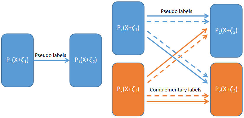
Figure 1. The difference between FixMatch (Sohn et al., 2020) and CLS. Left: FixMatch, where a prediction on the weakly-augmented sample ($X+\zeta_{1}$) generates a pseudo label for a strong augmentation of the same sample ($X+\zeta_{2}$) to learn from. Right: CLS, where two parallel networks generate both pseudo labels and complementary labels for themselves and each other. In some sense, supervision from the other network serves as a regularizer to mitigate the confirmation bias, while complementary labels support negative learning to boost performance further.

Researches on SSL usually start from some intuitive assumptions like smoothness, low-density, etc. For example, based on the smoothness assumption — “If two data points in a high-density region are close, then so should be the corresponding outputs” (Chapelle et al., 2009), consistency-based methods impose different consistency constraints over augmented inputs or perturbed networks (Srivastava et al., 2014) to enforce that the model prediction is invariant against data augmentations and proximity in the latent space. In this type of approaches (Sajjadi et al., 2016; Miyato et al., 2018; Xie et al., 2020a), the Teacher-Student structure is commonly used explicitly or implicitly to force the student to produce an output consistent with the teacher for the perturbed inputs. Similarly, low-entropy (i.e., high-confidence) regularization is employed to meet the low-density assumption. To encourage low-density separation between classes (Grandvalet and Bengio, 2004), Pseudo-Label (Lee et al., 2013), a self-training approach (McClosky et al., 2006; Mukherjee and Awadallah, 2020; Xie et al., 2020b), generates pseudo labels for unlabeled images based on the model’s class predictions and then selects high-confidence pairs (unlabeled images and their pseudo labels) to expand the training set. Self-training methods can be interpreted as a particular case of the Teacher-Student paradigm, where the teacher is a particular function of the student according to some predefined rules. Such rules include directly copying the student’s parameters (Rasmus et al., 2015), adopting an exponential moving average of the previous iterations (Laine and Aila, 2016; Tarvainen and Valpola, 2017), or designing a specific loss to optimize the teacher’s parameters (Pham et al., 2021). Furthermore, building on the respective advances in pseudo-labeling and consistency-based methods, current state-of-the-art methods tend to be a combination of these two types of methods. FixMatch (Sohn et al., 2020) uses the pseudo label of a weakly-augmented image to supervise the prediction of the same image under strong augmentation. MixMatch (Berthelot et al., 2019b) averages the estimations on multiple augmentations and produces the training target of the consistency regularization by applying a temperature sharpening function over the estimations.

Despite the strong performance of self-training methods and consistency-based methods, they all suffer from the problem of confirmation bias (Arazo et al., 2020), that is, if the teacher/pseudo labels are inaccurate, training the student/model itself under the misleading guidance may lead to significant performance degradation (Tarvainen and Valpola, 2017). To alleviate this problem, we propose a framework, namely cross labeling supervision (CLS), which contains three modifications to FixMatch (Sohn et al., 2020). (1) The first is the generation of complementary labels to support negative learning (Kim et al., 2019), which reduces the risk of providing wrong information since the chance of selecting the ground truth label as a complementary label is relatively low. Empirically, the additional generated complementary labels can help to calibrate incorrect predictions compared to only using pseudo labels as supervised signals. For ease of expression, pseudo labels and complementary labels are collectively referred to as artificial labels in this paper. (2) The second is a sample re-weighting mechanism to down-weight low-confidence artificial labels. Unlike FixMatch (Sohn et al., 2020), which sets a confidence threshold to completely filter out low-confidence pseudo labels, the advantage of using soft re-weighting is that the network can still learn from low-confidence labels for better generalization. (3) Inspired by co-training (Blum and Mitchell, 1998), we propose to exploit the disagreement of two independent models to achieve a complementary effect and avoid memorizing the inaccurate self-labeling samples. Specifically, two identical networks with different initializations are trained simultaneously, and they mitigate the confirmation bias of self-labeling by exchanging high-confidence artificial labels. Thanks to the development of parallel technology, training two networks simultaneously adds little computational overhead. Figure 1 demonstrates the difference between FixMatch (Sohn et al., 2020) and CLS.

In summary, the key contributions of this work include the following:

• We propose to tackle the confirmation bias problem, which is prevalent in self-training SSL methods and can lead to performance bottlenecks. The proposed CLS combines the advantages of negative learning and co-training to cope with this issue.

• While the previous SSL approaches mainly adopt threshold truncation to remove the influence of low-confidence pseudo labels; we propose a soft re-weighting method to quantify the quality of artificial labels and enhance the performance by improving label utilization.

• Comprehensive experiments demonstrate that CLS surpasses its SSL counterparts by significant margins on commonly used benchmark datasets CIFAR-10 and CIFAR-100.

2. Method

In this section, we introduce the intuition and details of CLS, which aims to overcome the confirmation bias problem. The complete structure of the method is presented in Figure 2.

2.1. Notation

For a $C$-class classification problem, let $\mathcal{X}_{l}=\{(x_{i},y_{i})\}^{N_{l}}_{i=1}$ denote the labeled dataset with $N_{l}$ samples and $\mathcal{X}_{u}=\{(x_{i})\}^{N_{u}}_{i=1}$ denote the unlabeled dataset with $N_{u}$ samples. The difference between the two datasets is that the ground-truth label $y_{i}\in\{1,\ldots,C\}$ of input $x_{i}$ in $\mathcal{X}_{l}$ is available, whereas the corresponding labels in $\mathcal{X}_{u}$ are absent. The goal of an SSL algorithm is to optimize a classifier $f:X\rightarrow Y$, which predicts the probability distribution that the input belongs to different classes. The parameterization of the classifier is denoted by $\theta$, which is optimized by gradient descent:

(1) $$\theta_{t}\leftarrow\theta_{t-1}-\alpha\bigtriangledown_{\theta_{t-1}}L(\mathcal{X}_{l}\cup\mathcal{X}_{u};\theta_{t-1}),$$

where $t\in\{1,...,T\}$ is the iteration index, $\alpha$ represents the learning rate and $L(\mathcal{X}_{l}\cup\mathcal{X}_{u};\theta_{t-1})$ is a loss function to be specified.

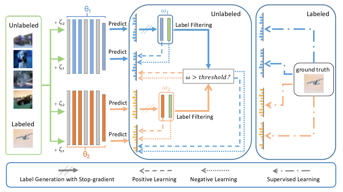
Figure 2. Structure overview of the CLS framework. The figure depicts a training batch with one labeled sample and four unlabeled samples. Before being fed into the two separate models, each sample will undergo both weak ($+\zeta_{2}$) and strong ($+\zeta_{1}$) augmentations. The prediction probability distribution for the weakly-augmented version is used to generate pseudo and complementary labels with corresponding sample weights, which are utilized to supervise the prediction on the strongly-augmented version via the positive and negative cross-entropy loss, respectively. When exchanging knowledge between the two models, only those labels with sample weights above a threshold are considered. As for the labeled sample, each model is trained to make its predictions match the ground-truth label.

2.2. Pseudo Label

In order to boost the classifier’s performance, a common way is to generate pseudo labels by self-labeling unlabeled samples, which are then incorporated with $\mathcal{X}_{l}$ to retrain the classifier. Such two procedures are normally run in an iterative manner. There are two major forms of pseudo labeling, i.e., hard labeling and soft labeling. Hard labeling (Lee et al., 2013) methods select the entries with the maximum probability as pseudo labels:

(2) $$\widetilde{y}_{i}=\mathop{\arg\max}\limits_{j\in\{1,\ldots,C\}}f(x_{i};\theta)_{j},$$

where $f(x_{i};\theta)\in\mathbb{R}^{C}$ represents the predicted probability distribution of input $x_{i}$, and $f(x_{i};\theta)_{j}$ denotes the corresponding probability of class $j$. Another approach to creating hard pseudo labels is to introduce a confidence threshold $\gamma\in[0,1]$ for truncation (Rizve et al., 2021; Sohn et al., 2020):

(3) $$\widetilde{y}_{ij}=\mathbbm{1}\left(f\left(x_{i};\theta\right)_{j}\geq\gamma\right),\ \text{for}\ j=1,2,\ldots,C,$$

where $\widetilde{y}_{ij}$ denotes the $j$-th entry of the refined multi-hot label for input $x_{i}$, and $\mathbbm{1}(\cdot)$ is the indicator function that outputs 1 if the inside condition is satisfied and 0 otherwise.

Different from hard labeling, which is generally non-differentiable, soft labeling applies a sharpening function (Berthelot et al., 2019b, a; Xie et al., 2020a) to enhance high-confident prediction while demoting low-confident ones. An example to refine the prediction distribution is given as follows:

(4) $$\widetilde{y}_{ij}=\frac{\left(f\left(x_{i};\theta\right)_{j}\right)^{\frac{1}{\epsilon}}}{\sum^{C}_{j^{\prime}=1}\left(f\left(x_{i};\theta\right)_{j^{\prime}}\right)^{\frac{1}{\epsilon}}},\text{for}\ j=1,2,\ldots,C,$$

where $\epsilon$ is a hyper-parameter that determines the “softness” of soft labeling. Note that as the temperature decreases, the soft pseudo labels become sharper, especially when $\epsilon\rightarrow 0$, the soft pseudo labels degrade to the hard pseudo labels.

2.3. Complementary Label

Although pseudo labels can be viewed as a form of entropy minimization that moves decision boundaries to low-density regions (Grandvalet and Bengio, 2004; Lee et al., 2013), inaccurate labels’ lack of calibration can lead to severe performance degradation due to the confirmation bias (Kim et al., 2019; Rizve et al., 2021). To remedy this, CLS generates not only pseudo labels to predict what category the current input most likely belongs to, but also complementary labels to indicate what category it would not belong to. Complementary labels allow for negative learning (Kim et al., 2019), which aims to prevent the model from overfitting to noisy data and accelerate model training. In contrast to hard pseudo labels, complementary labels corresponding to the low-confidence predictions can be obtained as follows:

(5) $$\overline{y}_{i}=\mathop{\arg\min}\limits_{j\in\{1,\ldots,C\}}f(x_{i};\theta)_{j}.$$

2.4. Cross Labeling Supervision

As discussed in Sec.1, learning from artificial labels generated by the classifier itself can suffer from the confirmation bias, and we propose two countermeasures in CLS.

2.4.1. Weighted Labeling

The first is to use sample re-weighting to tackle erroneous artificial labels. The intuition behind this is that the output softmax probability distributions with low entropy are more likely to produce accurate artificial labels. For example, a prediction of distribution $[0.01,0.99]$ is more promising to infer the ground-truth label than a prediction of $[0.45,0.55]$. Hence, it is highly desired to up-weight the more confident predictions and down-weight the less confident ones. To this end, we propose to assign adaptive sample weights to the artificial labels as follows:

(6) $$w_{i}=1-\frac{H\left(f\left(x_{i};\theta\right)\right)}{\log(C)},$$

where $H\left(f\left(x_{i};\theta\right)\right)=-\sum^{C}_{j=1}f\left(x_{i};\theta\right)_{j}\log\left(f\left(x_{i};\theta\right)_{j}\right)$ is the entropy of $f(x_{i};\theta)$ bounded in the interval $[0,\log(C)]$. Notice that $w_{i}\in[0,1]$ can reflect statistics regarding the confidence of artificial labels. Specifically, $w_{i}\rightarrow 0$ is equivalent to the uniform distribution (uncertain labels), whereas $w_{i}\rightarrow 1$ implies the one-hot distribution (deterministic labels).

Recall that hard labeling has become a typical configuration in SSL research due to its simplicity, generality, and ease of implementation. In this paper, we propose the re-weighting mechanism to maintain these advantages while mitigating the effects of mislabeling to enhance SSL performance. In particular, two modified cross-entropy loss functions are utilized as follows:

(7) $$\mathcal{L}_{P}(\theta,x_{i},w_{i},\widetilde{y}_{i}) =-w_{i}\sum^{C}_{j=1}\widetilde{y}_{ij}\log{f(x_{i};\theta)_{j}},$$

(8) $$\mathcal{L}_{N}(\theta,x_{i},w_{i},\overline{y}_{i}) =-w_{i}\sum^{C}_{j=1}\overline{y}_{ij}\log\left(1-{f\left(x_{i};\theta\right)_{j}}\right),$$

where $\widetilde{y}_{i}/\overline{y}_{i}$ is a given pseudo/complementary label with a discounted sample weight of $w_{i}$, and $\widetilde{y}_{ij}/\overline{y}_{ij}$ represents the $j$-th element of corresponding one-hot vectors.

2.4.2. Cross Labeling

Inspired by co-training (Blum and Mitchell, 1998; Han et al., 2018; Ke et al., 2019), we fuse knowledge from two collaborative models to alleviate the confirmation bias. To put this idea into practice, CLS trains two independent models simultaneously, adding little computational overhead due to parallel training at all time steps. However, the predictions of the two models may be inconsistent, and directly enforcing the consistency constraint between their output will mislead them to collapse into each other even though their initial states are different. Recall that diversity or different views play a non-trivial role in the success of co-training (Blum and Mitchell, 1998). In order to maintain the independence and difference between the two models, only high-confidence artificial labels are exchanged so that the supervised signals obtained from each other are always beneficial. Specifically, we introduce a weight threshold $\tau$ to filter out artificial labels whose sample weight is negligible.

2.4.3. Training Procedure

We briefly elaborate on the training process of CLS. It contains two independent models whose network weights are denoted by $\theta^{1}$ and $\theta^{2}$, respectively. Similar to FixMatch (Sohn et al., 2020), each network generates the targets from the weak-augmented samples:

(9) $$\widetilde{y}_{i}^{b} =\mathop{\arg\max}\limits_{j\in\{1,\ldots,C\}}f(x_{i}+\zeta_{2};\theta^{b})_{j},$$

(10) $$\overline{y}_{i}^{b} =\mathop{\arg\min}\limits_{j\in\{1,\ldots,C\}}f(x_{i}+\zeta_{2};\theta^{b})_{j},$$

(11) $$w_{i}^{b} =1-\frac{H\left(f\left(x_{i}+\zeta_{2};\theta^{b}\right)\right)}{\log(C)},$$

where $\zeta_{2}$ represents a weak augmentation strategy, and $b\in\{1,2\}$ is an identifier to indicate the corresponding network. With the generated artificial labels and corresponding sample weights, for a mini-batch $\mathcal{X}_{u}^{B}\subseteq\mathcal{X}_{u}$, we define the self-labeling loss function as

$$L_{self}^{b}(\mathcal{X}_{u}^{B})=\frac{1}{B}\sum_{x_{i}\in\mathcal{X}_{u}^{B}}\mathcal{L}_{P}(\theta^{b},x_{i} +\zeta_{1},w_{i}^{b},\widetilde{y}_{i}^{b})$$

(12) $$+\mathcal{L}_{N}(\theta^{b},x_{i} +\zeta_{1},w_{i}^{b},\overline{y}_{i}^{b}),$$

where $\zeta_{1}$ denotes the strong augmentation strategy, and $B$ is the mini-batch size.

As analyzed in Sec. 2.4.2, supervised signals from the weakly-augmented samples may not be adequate to calibrate the confirmation bias in self-training. To address this issue, we utilize cross labeling and define the co-labeling loss function concerning $\theta^{1}$ as

$$L_{co}^{1}(\mathcal{X}_{u}^{B}) =\frac{1}{B}\sum_{x_{i}\in\mathcal{X}_{u}^{B}}\mathbbm{1}(w_{i}^{2}>\tau)\mathcal{L}_{P}(\theta^{1},x_{i}+\zeta_{1},w_{i}^{2},\widetilde{y}_{i}^{2})$$

(13) $$+\mathbbm{1}(w_{i}^{2}>\tau)\mathcal{L}_{N}(\theta^{1},x_{i}+\zeta_{1},w_{i}^{2},\overline{y}_{i}^{2}),$$

where $\tau\in[0,1]$ is the weight threshold, and a larger value usually means that less but higher quality information is exchanged. In particular, cross labeling would fail when setting $\tau=1$ because $w_{i}^{b}$ ranges from 0 to 1, while setting $\tau=0$ may risk the model collapsing into each other. $L_{co}^{2}(\mathcal{X}_{u}^{B})$ can be calculated in a similar way to Eq. (2.4.3).

As for a labeled mini-batch $\mathcal{X}_{l}^{B}\subseteq\mathcal{X}_{l}$, both models are trained via a standard supervised classification as

(14) $$L_{sup}^{b}(\mathcal{X}_{l}^{B})=\frac{1}{B}\sum_{(x_{i},y_{i})\in\mathcal{X}_{l}^{B}}{\sum^{C}_{j=1}{y}_{ij}\log{f(x_{i};\theta^{b})_{j}}}.$$

Following FixMatch (Sohn et al., 2020), we consider different relative sizes of $\mathcal{X}_{u}$ and $\mathcal{X}_{l}$, which are denoted by $\mu$. Given $\mathcal{X}_{l}^{B}$ and $\mathcal{X}_{u}^{\mu B}$, network $\theta^{b}$ ($b\in\{1,2\}$) is optimized with the mixed loss in the form of

(15) $$L^{b}=L_{sup}^{b}(\mathcal{X}_{l}^{B})+\lambda_{1}L_{self}^{b}(\mathcal{X}_{u}^{\mu B})+\lambda_{2}L_{co}^{b}(\mathcal{X}_{u}^{\mu B}),$$

where $\lambda_{1}$ and $\lambda_{2}$ are the trade-off coefficients between various losses. The complete algorithm for CLS is presented in algorithm 1.

Input: $\mathcal{X}_{l}$: labeled dataset; $\mathcal{X}_{u}$: unlabeled dataset; $\mu$: unlabeled data ratio; $\tau$: weight threshold; $\lambda_{1}$/$\lambda_{2}$: self/co-labeling loss coefficient;  $\zeta_{1}$/$\zeta_{2}$: strong/weak augmentation strategy.

1 Initialize $\theta^{1}_{0}$ and $\theta^{2}_{0}$ with different random seeds;

2 for $t=1,\cdots,T$ do

3       Sample a mini-batch of size $B$ from $\mathcal{X}_{l}$: $\mathcal{X}_{l}^{B}$;

4       Sample a mini-batch of size $\mu B$ from $\mathcal{X}_{u}$: $\mathcal{X}_{u}^{\mu B}$;

       // Label generation

5       for $b=1,2$ do

6             Pseudo labels $\leftarrow$ Eq. (9) on $\mathcal{X}_{u}^{\mu B}$;

7             Complementary labels $\leftarrow$ Eq. (10) on $\mathcal{X}_{u}^{\mu B}$;

8             Sample weights $\leftarrow$ Eq. (11) on $\mathcal{X}_{u}^{\mu B}$;

9       end for

      // Loss calculation

10       for $b=1,2$ do

11             $L^{b}\leftarrow$ Eq. (15) on $\mathcal{X}_{l}^{B}\cup\mathcal{X}_{u}^{\mu B}$;

12       end for

      // Update $\theta_{1}$ and $\theta_{2}$ in parallel

13       $\theta_{t}^{1}\leftarrow\theta_{t-1}^{1}-\alpha\bigtriangledown_{\theta_{t-1}^{1}}L^{1}$;

14       $\theta_{t}^{2}\leftarrow\theta_{t-1}^{2}-\alpha\bigtriangledown_{\theta_{t-1}^{2}}L^{2}$;

15      

16 end for

Output: $\theta_{T}^{1}$ or $\theta_{T}^{2}$ for prediction.

Algorithm 1 CLS Algorithm

3. Experiments

Our experiments aim to answer the following questions:

• RQ1: How does CLS perform in standard benchmarks compared to prior state-of-the-art SSL algorithms?

• RQ2: What is the effect of each component in CLS?

• RQ3: How does CLS mitigate the confirmation bias?

• RQ4: How do different hyperparameters affect CLS?

3.1. Experimental Settings

3.1.1. Datasets

The benchmark datasets we used are CIFAR-10, CIFAR-100 (Krizhevsky et al., 2009), which both contain 50K training images and 10K test images of size 32 × 32 with respect to 10 and 100 class categories, respectively. Following the partition protocols of Fixmatch (Sohn et al., 2020), we experiment with three sizes of labeled images on those two datasets. To be specific, we divide the training set of CIFAR-10 into two groups, with 40, 250, and 4K samples randomly selected as the labeled set and the rest as the unlabeled set. CIFAR-100 is similarly divided, corresponding to 400, 2.5K, and 10K labeled samples. The prediction accuracy on the test set is adopted as the evaluation metric.

3.1.2. Baselines

We compare CLS against four groups of baselines. The vanilla baseline is supervised learning (SL) with data augmentation methods, e.g., RandAugment (RA) (Cubuk et al., 2020). This baseline is set to ensure that SL has a relatively fair comparison with those state-of-the-art SSL methods that leverage strong data augmentation methods. Note that the RA method is also applied to UPS (Rizve et al., 2021), UDA (Xie et al., 2020a), and all hybrid methods. The second group of baselines consists of two self-training methods that generate pseudo labels for the unlabeled set, where high-confidence labels are selected to expand the labeled set. Specifically, Pseudo-Label (Lee et al., 2013) generates pseudo labels without using data augmentation methods, while UPS (Rizve et al., 2021) creates additional complementary labels for the low-confidence samples in the unlabeled dataset. The third group contains consistency regularization methods, where $\Pi$-model (Rasmus et al., 2015) and Mean Teacher (Tarvainen and Valpola, 2017) are two classic benchmarks while UDA (Xie et al., 2020a) represents the state-of-the-art consistency training method. Similar to CLS, recent hybrid methods incorporate self-training with consistency training. Three state-of-the-art methods are selected for comparison, i.e., MixMatch (Berthelot et al., 2019b), ReMixMatch (Berthelot et al., 2019a), and FixMatch (Sohn et al., 2020).

3.1.3. Implementation Details

We implement our method based on the PyTorch (Paszke et al., 2019) framework, i.e., PyTorch 1.3. In our experiments, all baselines share the same backbone and dataset partitioning. For CIFAR-10, the backbone architecture adopted is a WideResNet-28-2 (Zagoruyko and Komodakis, 2016) with 1.45 million parameters, while a WideResNet-28-8 (Zagoruyko and Komodakis, 2016) with 23.40 million parameters is used for CIFAR-100. This setting is commonly used by previous works (Rizve et al., 2021; Sohn et al., 2020; Berthelot et al., 2019b). We utilize the SGD optimizer (Bottou, 2012) in conjunction with Nesterov momentum (Tang et al., 2018) for network training. Following FixMatch (Sohn et al., 2020), the cosine learning rate decay schedule is used for learning rate adjustment. In all of our experiments, weak augmentation is realized with a standard flip-and-shift augmentation strategy, while the strong augmentation strategy is RandAugment (RA) (Cubuk et al., 2020). All experiments are trained on NVIDIA Tesla V100 GPUs, and the default hyper-parameter configuration of CLS is {$\alpha=0.03,\mu=8,B=64,T=300,\tau=0.85,\lambda_{1}=2,\lambda_{2}=1$}. Refer to Appendix for more details.

Table 1. Classification accuracy (%) of CLS and various baselines over 4 runs on 2 standard benchmarks, the higher, the better.

Category	Method	CIFAR-10			CIFAR-100
		40 labels	250 labels	4k labels	400 labels	2.5k labels	10k labels
Vanilla baseline	SL w/ RA (Cubuk et al., 2020)	35.96$\pm$0.88	60.78$\pm$0.65	87.36$\pm$0.32	20.43$\pm$0.22	46.93$\pm$0.47	68.42$\pm$0.33
Self-Training	Pseudo-Label (Lee et al., 2013)	-	51.31$\pm$0.66	84.62$\pm$0.38	-	43.26$\pm$0.43	65.78$\pm$0.29
	UPS (Rizve et al., 2021)	-	78.39$\pm$0.88	89.59$\pm$0.64	-	52.34$\pm$0.45	68.77$\pm$0.25
Consistency Training	$\Pi$-model (Rasmus et al., 2015)	-	46.24$\pm$5.48	86.41$\pm$0.56	-	43.85$\pm$0.68	63.53$\pm$0.16
	Mean Teacher (Tarvainen and Valpola, 2017)	-	69.44$\pm$3.11	91.22$\pm$0.21	-	47.19$\pm$0.62	66.21$\pm$0.33
	UDA (Xie et al., 2020a)	71.63$\pm$6.72	91.10$\pm$1.15	95.08$\pm$0.22	41.24$\pm$0.92	66.89$\pm$0.32	75.23$\pm$0.45
Hybrid methods	MixMatch (Berthelot et al., 2019b)	54.65$\pm$9.78	89.21$\pm$1.22	93.66$\pm$0.18	33.43$\pm$2.14	61.14$\pm$0.67	72.17$\pm$0.42
	ReMixMatch (Berthelot et al., 2019a)	81.94$\pm$7.63	94.48$\pm$0.36	95.26$\pm$0.14	54.88$\pm$2.33	73.37$\pm$0.41	76.88$\pm$0.63
	FixMatch (Sohn et al., 2020)	88.29$\pm$3.44	94.85$\pm$0.76	95.73$\pm$0.15	51.81$\pm$2.16	72.73$\pm$0.66	77.33$\pm$0.24
Hybrid methods	CLS	91.82$\pm$1.77	95.55$\pm$0.33	96.28$\pm$0.06	55.91$\pm$1.12	74.06$\pm$0.28	79.27$\pm$0.16

3.2. Comparison with Baselines

Table 1 shows the results on CIFAR-10 and CIFAR-100 with different sizes of the labeled dataset. We report the averaged test accuracy and corresponding standard deviation over four runs. All hybrid methods consistently outperform the vanilla baseline by substantial margins across all settings, showing the promise of SSL methods. It is worth mentioning that the vanilla baseline can perform on par with traditional SSL methods that do not use data augmentation, i.e., Pseudo-Label (Lee et al., 2013), $\Pi$-model (Rasmus et al., 2015), and Mean Teacher (Tarvainen and Valpola, 2017). Such results prove the necessity and effectiveness of advanced data augmentation methods. Furthermore, CLS achieves state-of-the-art performances in all settings, which demonstrates the validity of our method, especially in highly label-scarce settings. Specifically, we surpass the vanilla baseline by considerable margins of 55.86% and 35.48% accuracy on CIFAR-10 with 40 labels and CIFAR-100 with 400 labels. More importantly, although CLS can be viewed as an extension of FixMatch (Sohn et al., 2020), stable performance gains achieved by CLS on both datasets suggest that the modifications to FixMatch are effective.

Table 2. Classification accuracy (%) of several variants of CLS on CIFAR-10 and CIFAR-100 over 4 runs.

Method	CIFAR-10			CIFAR-100
	40 labels	250 labels	4k labels	400 labels	2.5k labels	10k labels
FixMatch	$88.29\pm 3.44$	$94.85\pm 0.76$	$95.73\pm 0.15$	$51.81\pm 2.16$	$72.73\pm 0.66$	$77.33\pm 0.24$
FixMatch w/ NL	$89.58\pm 2.11$	$94.91\pm 0.87$	$95.89\pm 0.07$	$52.76\pm 1.61$	$73.21\pm 0.46$	$77.45\pm 0.54$
FixMatch w/ RW	$89.87\pm 1.98$	$94.89\pm 1.06$	$95.82\pm 0.11$	$52.43\pm 2.87$	$73.37\pm 0.43$	$77.75\pm 0.32$
FixMatch w/ (NL & RW)	$90.24\pm 1.87$	94.98 $\pm$ 0.65	$96.02\pm 0.29$	$53.42\pm 1.33$	73.49 $\pm$ 0.35	$78.31\pm 0.18$
CLS w/o NL	$90.61\pm 2.64$	$94.87\pm 1.11$	$96.03\pm 0.09$	$52.87\pm 1.31$	$72.78\pm 0.39$	$78.55\pm 0.25$
CLS w/o RW	90.89 $\pm$ 2.57	$94.91\pm 0.87$	96.05 $\pm$ 0.07	53.59 $\pm$ 1.95	$73.34\pm 0.41$	78.69 $\pm$ 0.33
CLS	91.82 $\pm$ 1.77	95.55 $\pm$ 0.33	96.28 $\pm$ 0.06	55.91 $\pm$ 1.12	74.06 $\pm$ 0.28	79.27 $\pm$ 0.16

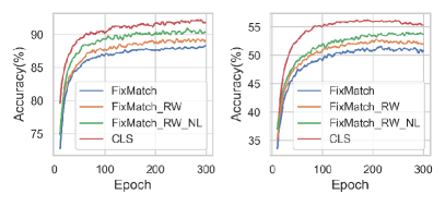
Figure 3. The classification accuracy of FixMatch and three variants of CLS. Left: Test accuracy on CIFAR-10 with 40 labels. Right: Test accuracy on CIFAR-100 with 400 labels. The gap between the four curves indicates that the introduction of each component brings a performance improvement.

3.3. Ablation Study

Our paper suggests a comprehensive framework for SSL consisting of the following essential ingredients: (1) using sample re-weighting mechanism, short for RW; (2) generating extra complementary labels for negative learning, abbreviated as NL; (3) exchanging artificial labels for cross supervision. To investigate the strength of each component in CLS, we conducted an analysis that reveals the performance differences when using different combinations of these components during training. Variants include modifications to FixMatch and the removal of NL or RW from the CLS. All variants use the default configuration of CLS, except for changes in specific components. Table 2 presents the results of all experiments performed for the analysis.

As shown in Table 2, compared to FixMatch, all variants achieve performance improvements, demonstrating the positive effect of each component. It is noteworthy that significant performance gains are shown when there are fewer labeled images, especially in the two cases of CIFAR-10 with 40 labels and CIFAR-100 with 400 labels, where only 4 labels are assigned to each class on both datasets. Specifically, CLS improved the average accuracy from 88.29% to 91.82% on CIFAR-10 with 40 labels and from 51.81% to 55.91% on CIFAR-100 with 400 labels. To explore whether the efficacy of different components can be superimposed, we visualized the learning curves of four variants in label-scarce settings. As shown in Figure 3, the increase in accuracy suggests that the three components of CLS complement each other, and their combination can yield better accuracy than omitting one or more elements.

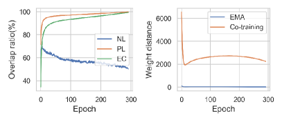
Figure 4. Illustration of the cross labeling. Left: While the overlap of pseudo labels (PL) generated by the two networks and the exchange ratio (EC) of labels increases over time, the overlap of complementary labels (NL) predicted by the two networks remains at a relatively low level. Right: An exponential moving average (EMA) of network $\theta^{1}$ has similar weights to itself, while the weights of $\theta^{1}$ and $\theta^{2}$ keep a certain distance.

3.4. Analysis of Cross Labeling

As discussed in Sec. 2.4.2, the confirmation bias is an inevitable obstacle to self-labeling methods. For instance, using artificial labels from weakly-augmented samples as targets for strongly-augmented samples may risk overfitting inaccurate labels since the predictions for the strongly-augmented samples come from the same network. In addition, recent self-labeling methods generally use exponential moving average (EMA) techniques to provide more stable predictions (Tarvainen and Valpola, 2017). However, the coupling effect of EMA models is likely to result in an accumulation of errors and make misclassification irreversible by enforcing the current predictions to match those of the EMA. In our work, we propose to use cross labeling, a specific variant of co-training (Blum and Mitchell, 1998), to address this issue.

To visualize why cross-labeling is effective, we calculated the proportion of identical artificial labels generated by the two models and the ratio used for exchange. We also calculated the Euclidean distance of different model weights. The results are visualized in Figure 4. As expected, the predictions of the two models become gradually consistent as the training proceeds. However, the weights of the two collaborative models remain pretty different and can provide a certain percentage of inconsistent complementary labels to complement each other’s training.

Figure 5. Test error rate on CIFAR-10 with 250 labels. (a) Varying self-labeling loss coefficient $\lambda_{1}$. (b) Varying co-labeling loss coefficient $\lambda_{2}$. (c) Varying the ratio of unlabeled data. (d) Varying the weight threshold for cross labeling. In each experiment, we varied one hyper-parameter, and used the default hyper-parameters for the rest. Error rate of CLS with the default setting is in dotted line.

3.5. Hyper-parameter Study

CLS has four key hyper-parameters: the trade-off coefficients between various losses ($\lambda_{1}$ and $\lambda_{2}$), the ratio of unlabeled samples to labeled samples in each mini-batch ($\mu$), and the weight-threshold hyper-parameter $\tau$ for exchanging artificial labels between two networks. To assess the sensitivity of various aspects of CLS, we ran experiments on CIFAR-10 with 250 labels, varying one hyper-parameter at a time while keeping the others fixed.

Necessity of the self-labeling loss (Figure 5(a)). When the self-labeling loss is given small coefficients, performance degradation can be observed. In particular, when the self-supervised loss is removed, i.e., $\lambda_{1}=0$, the error rate increases by 1.25%, which is a remarkable gap on CIFAR-10 with 250 labels. On the other hand, in the case of $\lambda_{1}\geq 1$, the performance of CLS is relatively stable.

Effectiveness of the co-labeling loss (Figure 5(b) and  5(d)). Similar to the self-labeling loss, performance decreases with the removal of the co-labeling loss ($\lambda_{2}=0$ or $\tau=1$). An interesting finding is that the performance also degrades when the coefficient of the co-labeling loss is too large ($\lambda_{2}\geq 2$). This is because the two networks may disagree on certain predictions, and pseudo labels provided by the other network may not be accurate. However, this property also allows the co-labeling loss to be treated as a regularization term to prevent overfitting.

CLS prefers larger values of $\mu$ (Figure 5(c)). A significant decrease in error rates can be observed with the increase of unlabeled data, which is in agreement with the conclusions in UDA (Xie et al., 2020a) and FixMatch (Sohn et al., 2020).

4. Related Work

Semi-supervised learning is a mature field with a vast diversity of approaches. In this review, we focus on methods closely related to CLS.

4.1. Self-training Methods

The idea of self-training originates from (McLachlan, 1975), which derives a paradigm that leverages the model to generate artificial labels for unlabeled data and then utilizes artificial labels to re-optimize the model itself, with the two processes alternating iteratively. Due to its generality and simplicity, self-training has been widely used in many fields, such as image classification (Xie et al., 2020b), object detection (Yang et al., 2021), etc. Pseudo-labeling (Lee et al., 2013) is a special case of self-training and is usually used in conjunction with confidence-based thresholds, i.e., only unlabeled samples with prediction confidence above a certain threshold are used to supplement the training set. As described in (Grandvalet and Bengio, 2004), pseudo-labeling is a form of entropy minimization that can produce better results, and it has become a standard component of the SSL algorithm pipeline. Although pseudo-labeling has achieved excellent performance in various tasks, some studies suggested that it can suffer from the vulnerability to inaccurate pseudo-labels (Arazo et al., 2020), especially in large-sized label space. In addition to the confidence-based threshold mechanism, another common solution to mitigate the effects of noisy labels is sample reweighting (Kumar et al., 2010), where high-confidence samples are granted greater weights, and vice versa. Recently, UPS (Rizve et al., 2021) introduces the concept of negative learning (Kim et al., 2019) and generates complementary labels when pseudo-labels are not sufficiently confident.

4.2. Consistency Regularization

The idea behind consistency regularization in SSL literature is to require the classifier to be robust to stochastic transformations and perturbations (Sajjadi et al., 2016), which was first proposed by (Bachman et al., 2014). To this end, input perturbation methods (Sajjadi et al., 2016) impose consistency constraints on the predictions between different augmentations of the same sample so that the decision bound can lie in the low-density region. On the other hand, feature perturbation methods perturb the model structure (e.g., using dropout (Srivastava et al., 2014)) or utilize multiple models (Ke et al., 2019) to get multiple outputs on which consistency constraints are imposed. To be specific, “$\Pi$-Model” (Rasmus et al., 2015) forces the predictions of two different augmentations of the same image to match each other. Temporal Ensembling (Laine and Aila, 2016) and its extension Mean Teacher (Tarvainen and Valpola, 2017) use an exponential moving average of previous predictions and model parameters to generate supervision targets for unlabeled data, respectively. Recently, the combination of consistency regularization and pseudo-labeling has gained more and more attention. In MixMatch (Berthelot et al., 2019b), pseudo-labels are generated by averaging the predictions of different augmentations of the same sample. ReMixMatch (Berthelot et al., 2019a) and UDA (Xie et al., 2020a) further extend this idea by dividing the set of augmentations into strong and weak augmentations, while FixMatch (Sohn et al., 2020) leverages the model’s predictions on weakly-augmented unlabeled samples to create pseudo-labels for the strongly-augmented versions of the same samples.

However, all the methods mentioned above are self-labeling approaches. An obvious obstacle in such methods is the confirmation bias (Arazo et al., 2020): the performance of self-labeling methods is restricted by the inaccurate artificial labels. To resolve this issue, our method generates adaptive sample weights for artificial labels, where samples with low confidence are given small weights so that the effect of inaccurate labels can be effectively reduced. In addition, we borrow the idea of co-training (Han et al., 2018; Yu et al., 2019; Ke et al., 2019) to exchange high-confidence labels between two collaborative networks. Similar to UPS (Rizve et al., 2021), CLS also generates complementary labels to improve robustness to inaccurate artificial labels.

5. Conclusion

In this paper, we proposed the Cross Labeling Supervision (CLS) method for SSL. Key to CLS is the idea that one network learning from the supervision of another independent network can help alleviate the problem of confirmation bias. The learning process of CLS consists of two main steps: reweighting the artificial labels (both pseudo labels and complementary labels) according to their prediction confidence and exchanging reliable artificial labels between the two different initialized networks for co-training. Experiments on standard SSL benchmarks show that CLS outperforms other state-of-the-art methods.

References

- (1)
- Arazo et al. (2020) Eric Arazo, Diego Ortego, Paul Albert, Noel E O’Connor, and Kevin McGuinness. 2020. Pseudo-labeling and confirmation bias in deep semi-supervised learning. In 2020 International Joint Conference on Neural Networks (IJCNN). IEEE, 1–8.
- Bachman et al. (2014) Philip Bachman, Ouais Alsharif, and Doina Precup. 2014. Learning with pseudo-ensembles. Advances in neural information processing systems 27 (2014), 3365–3373.
- Berthelot et al. (2019a) David Berthelot, Nicholas Carlini, Ekin D Cubuk, Alex Kurakin, Kihyuk Sohn, Han Zhang, and Colin Raffel. 2019a. ReMixMatch: Semi-Supervised Learning with Distribution Matching and Augmentation Anchoring. In International Conference on Learning Representations.
- Berthelot et al. (2019b) David Berthelot, Nicholas Carlini, Ian Goodfellow, Nicolas Papernot, Avital Oliver, and Colin A Raffel. 2019b. MixMatch: A Holistic Approach to Semi-Supervised Learning. Advances in Neural Information Processing Systems 32 (2019), 5049–5059.
- Blum and Mitchell (1998) Avrim Blum and Tom Mitchell. 1998. Combining labeled and unlabeled data with co-training. In Proceedings of the eleventh annual conference on Computational learning theory. 92–100.
- Bottou (2012) Léon Bottou. 2012. Stochastic gradient descent tricks. In Neural networks: Tricks of the trade. Springer, 421–436.
- Chapelle et al. (2009) Olivier Chapelle, Bernhard Scholkopf, and Alexander Zien. 2009. Semi-supervised learning (chapelle, o. et al., eds.; 2006)[book reviews]. IEEE Transactions on Neural Networks 20, 3 (2009), 542–542.
- Chen et al. (2021) Xiaokang Chen, Yuhui Yuan, Gang Zeng, and Jingdong Wang. 2021. Semi-Supervised Semantic Segmentation with Cross Pseudo Supervision. In Proceedings of the IEEE/CVF Conference on Computer Vision and Pattern Recognition. 2613–2622.
- Cubuk et al. (2020) Ekin D Cubuk, Barret Zoph, Jonathon Shlens, and Quoc V Le. 2020. Randaugment: Practical automated data augmentation with a reduced search space. In Proceedings of the IEEE/CVF Conference on Computer Vision and Pattern Recognition Workshops. 702–703.
- Grandvalet and Bengio (2004) Yves Grandvalet and Yoshua Bengio. 2004. Semi-supervised learning by entropy minimization. In Proceedings of the 17th International Conference on Neural Information Processing Systems. 529–536.
- Han et al. (2018) Bo Han, Quanming Yao, Xingrui Yu, Gang Niu, Miao Xu, Weihua Hu, Ivor W Tsang, and Masashi Sugiyama. 2018. Co-teaching: robust training of deep neural networks with extremely noisy labels. In Proceedings of the 32nd International Conference on Neural Information Processing Systems. 8536–8546.
- Ke et al. (2019) Zhanghan Ke, Daoye Wang, Qiong Yan, Jimmy Ren, and Rynson WH Lau. 2019. Dual student: Breaking the limits of the teacher in semi-supervised learning. In Proceedings of the IEEE/CVF International Conference on Computer Vision. 6728–6736.
- Kim et al. (2019) Youngdong Kim, Junho Yim, Juseung Yun, and Junmo Kim. 2019. Nlnl: Negative learning for noisy labels. In Proceedings of the IEEE/CVF International Conference on Computer Vision. 101–110.
- Krizhevsky et al. (2009) Alex Krizhevsky, Geoffrey Hinton, et al. 2009. Learning multiple layers of features from tiny images. (2009).
- Kumar et al. (2010) M Kumar, Benjamin Packer, and Daphne Koller. 2010. Self-paced learning for latent variable models. Advances in neural information processing systems 23 (2010), 1189–1197.
- Laine and Aila (2016) Samuli Laine and Timo Aila. 2016. Temporal ensembling for semi-supervised learning. arXiv preprint arXiv:1610.02242 (2016).
- Lee et al. (2013) Dong-Hyun Lee et al. 2013. Pseudo-label: The simple and efficient semi-supervised learning method for deep neural networks. In Workshop on challenges in representation learning, ICML, Vol. 3. 896.
- Li et al. (2017) Wen Li, Limin Wang, Wei Li, Eirikur Agustsson, and Luc Van Gool. 2017. WebVision Database: Visual Learning and Understanding from Web Data. CoRR (2017).
- McClosky et al. (2006) David McClosky, Eugene Charniak, and Mark Johnson. 2006. Effective self-training for parsing. In Proceedings of the Human Language Technology Conference of the NAACL, Main Conference. 152–159.
- McLachlan (1975) Geoffrey J McLachlan. 1975. Iterative reclassification procedure for constructing an asymptotically optimal rule of allocation in discriminant analysis. J. Amer. Statist. Assoc. 70, 350 (1975), 365–369.
- Miyato et al. (2018) Takeru Miyato, Shin-ichi Maeda, Masanori Koyama, and Shin Ishii. 2018. Virtual adversarial training: a regularization method for supervised and semi-supervised learning. IEEE transactions on pattern analysis and machine intelligence 41, 8 (2018), 1979–1993.
- Mukherjee and Awadallah (2020) Subhabrata Mukherjee and Ahmed Awadallah. 2020. Uncertainty-aware self-training for few-shot text classification. Advances in Neural Information Processing Systems 33 (2020).
- Paszke et al. (2019) Adam Paszke, Sam Gross, Francisco Massa, Adam Lerer, James Bradbury, Gregory Chanan, Trevor Killeen, Zeming Lin, Natalia Gimelshein, Luca Antiga, et al. 2019. Pytorch: An imperative style, high-performance deep learning library. Advances in neural information processing systems 32 (2019), 8026–8037.
- Pham et al. (2021) Hieu Pham, Zihang Dai, Qizhe Xie, and Quoc V Le. 2021. Meta pseudo labels. In Proceedings of the IEEE/CVF Conference on Computer Vision and Pattern Recognition. 11557–11568.
- Rasmus et al. (2015) Antti Rasmus, Mathias Berglund, Mikko Honkala, Harri Valpola, and Tapani Raiko. 2015. Semi-supervised Learning with Ladder Networks. Advances in Neural Information Processing Systems 28 (2015), 3546–3554.
- Rizve et al. (2021) Mamshad Nayeem Rizve, Kevin Duarte, Yogesh S Rawat, and Mubarak Shah. 2021. In Defense of Pseudo-Labeling: An Uncertainty-Aware Pseudo-label Selection Framework for Semi-Supervised Learning. In International Conference on Learning Representations. https://openreview.net/forum?id=-ODN6SbiUU
- Russakovsky et al. (2015) Olga Russakovsky, Jia Deng, Hao Su, Jonathan Krause, Sanjeev Satheesh, Sean Ma, Zhiheng Huang, Andrej Karpathy, Aditya Khosla, Michael Bernstein, et al. 2015. Imagenet large scale visual recognition challenge. International journal of computer vision 115, 3 (2015), 211–252.
- Sajjadi et al. (2016) Mehdi Sajjadi, Mehran Javanmardi, and Tolga Tasdizen. 2016. Regularization with stochastic transformations and perturbations for deep semi-supervised learning. Advances in neural information processing systems 29 (2016), 1163–1171.
- Sohn et al. (2020) Kihyuk Sohn, David Berthelot, Nicholas Carlini, Zizhao Zhang, Han Zhang, Colin A Raffel, Ekin Dogus Cubuk, Alexey Kurakin, and Chun-Liang Li. 2020. FixMatch: Simplifying Semi-Supervised Learning with Consistency and Confidence. Advances in Neural Information Processing Systems 33 (2020).
- Srivastava et al. (2014) Nitish Srivastava, Geoffrey Hinton, Alex Krizhevsky, Ilya Sutskever, and Ruslan Salakhutdinov. 2014. Dropout: a simple way to prevent neural networks from overfitting. The journal of machine learning research 15, 1 (2014), 1929–1958.
- Tang et al. (2018) Shenghao Tang, Changqing Shen, Dong Wang, Shuang Li, Weiguo Huang, and Zhongkui Zhu. 2018. Adaptive deep feature learning network with Nesterov momentum and its application to rotating machinery fault diagnosis. Neurocomputing 305 (2018), 1–14.
- Tarvainen and Valpola (2017) Antti Tarvainen and Harri Valpola. 2017. Mean teachers are better role models: Weight-averaged consistency targets improve semi-supervised deep learning results. Advances in Neural Information Processing Systems 30 (2017).
- Xie et al. (2020a) Qizhe Xie, Zihang Dai, Eduard Hovy, Thang Luong, and Quoc Le. 2020a. Unsupervised Data Augmentation for Consistency Training. Advances in neural information processing systems 33 (2020).
- Xie et al. (2020b) Qizhe Xie, Minh-Thang Luong, Eduard Hovy, and Quoc V Le. 2020b. Self-training with noisy student improves imagenet classification. In Proceedings of the IEEE/CVF Conference on Computer Vision and Pattern Recognition. 10687–10698.
- Yang et al. (2021) Qize Yang, Xihan Wei, Biao Wang, Xian-Sheng Hua, and Lei Zhang. 2021. Interactive self-training with mean teachers for semi-supervised object detection. In Proceedings of the IEEE/CVF Conference on Computer Vision and Pattern Recognition. 5941–5950.
- Yu et al. (2019) Xingrui Yu, Bo Han, Jiangchao Yao, Gang Niu, Ivor Tsang, and Masashi Sugiyama. 2019. How does disagreement help generalization against label corruption?. In International Conference on Machine Learning. PMLR, 7164–7173.
- Zagoruyko and Komodakis (2016) Sergey Zagoruyko and Nikos Komodakis. 2016. Wide Residual Networks. In British Machine Vision Conference 2016. British Machine Vision Association.