Causal inference with recurrent and competing events

Abstract.

Many research questions concern treatment effects on outcomes that can recur several times in the same individual. For example, medical researchers are interested in treatment effects on hospitalizations in heart failure patients and sports injuries in athletes. Competing events, such as death, complicate causal inference in studies of recurrent events because once a competing event occurs, an individual cannot have more recurrent events. Several statistical estimands have been studied in recurrent event settings, with and without competing events. However, the causal interpretations of these estimands, and the conditions that are required to identify these estimands from observed data, have yet to be formalized. Here we use a counterfactual framework for causal inference to formulate several causal estimands in recurrent event settings, with and without competing events. When competing events exist, we clarify when commonly used classical statistical estimands can be interpreted as causal quantities from the causal mediation literature, such as (controlled) direct effects and total effects. Furthermore, we show that recent results on interventionist mediation estimands allow us to define new causal estimands with recurrent and competing events that may be of particular clinical relevance in many subject matter settings. We use causal directed acyclic graphs and single world intervention graphs to illustrate how to reason about identification conditions for the various causal estimands using subject matter knowledge. Furthermore, using results on counting processes, we show how our causal estimands and their identification conditions, which are articulated in discrete time, converge to classical continuous-time counterparts in the limit of fine discretizations of time. Finally, we propose several estimators and establish their consistency for the various identifying functionals.

1. Introduction

Practitioners and researchers are often interested in treatment effects on outcomes that can recur in the same individual over time. Such outcomes include hospitalizations in heart failure patients (Anker and McMurray, 2012), fractures in breast cancer patients with skeletal metastases (Chen and Cook, 2004) and rejection episodes in recipients of kidney transplants (Cook and Lawless, 1997). However, in many studies of recurrent events, individuals may also experience competing events, such as death. These events may substantially complicate causal inference.

For example, consider investigators concerned with the effects of over-treatment of older adults with antihypertensive agents and aspirin. Over-treatment might lead to episodes of syncope (dizziness) caused by blood pressure becoming too low (in turn, possibly leading to injurious falls). Suppose these investigators conduct a randomized controlled trial in a sample of patients admitted to nursing homes with a history of cardiovascular disease and currently taking antihypertensives and aspirin. Patients are then randomly assigned to either discontinue or to continue both treatments (a similar intervention is considered in Reeve et al. (2020)). Assume no participant moves out of the nursing home or disenrolls from the study. After 1000 days, the investigators calculate the average number of syncope episodes in each arm and find that this average is lower in the treatment discontinuation arm compared to the continuation arm. However, they also calculate the proportion of deaths in each arm and find that mortality was higher in the discontinuation arm compared to the continuation arm.

In this example, all-cause mortality is a competing event for the outcome of interest (number of recurrent syncope episodes) because once an individual dies they cannot subsequently experience syncope. Due to the randomized design and the fact that no participant was lost to follow-up, the analysis these investigators conducted indeed has a “causal” interpretation: their results support an average protective effect of treatment discontinuation on the number of syncope episodes. However, analogous to previous arguments in the case where the outcome of interest is an incident (rather than a recurrent) event subject to competing events (Young et al., 2020; Stensrud et al., 2020b), this “protection” is difficult to interpret in light of the finding that mortality risk is increased by treatment discontinuation. The increased number of syncope episodes in the discontinuation treatment arm might only be due to the treatment effect on mortality.

The importance of characterizing the causal interpretation of statistical estimands is increasingly acknowledged (European Medicines Agency, 2020). In a series of articles by the Recurrent Event Qualification Opinion Consortium (Schmidli et al., 2021; Wei, ; Fritsch et al., 2021), six candidate causal estimands were proposed in recurrent event settings with competing events, defined by counterfactual contrasts under different treatment scenarios in the following: 1) the expected number of events in the study population; 2) the expectation over a composite of the recurrent and competing events in the study population; 3) the expected number of events under an intervention which prevents the competing event from occurring in the study population; 4) the expected number of events in a subset of the study population consisting of the principal stratum of individuals that would survive regardless of treatment; 5) the ratio of the expected number of recurrences to the restricted mean survival by the end of follow-up in the study population and 6) the ratio of the expectation over a composite of the recurrent and competing events to the restricted mean survival by the end of follow-up in the study population.

In addition to defining these various counterfactual estimands,  Schmidli et al. (2021) considered some aspects of their differences in interpretation, as well as, for some of the estimands, approaches to statistical analysis. However, they did not consider assumptions needed to identify any of these counterfactual estimands in a given study with a function of the observed data. Once a causal estimand is chosen, this identification step is required to justify a choice of approach to statistical analysis. Furthermore, Schmidli et al. (2021) did not consider how underlying questions about treatment mechanism may be important to the choice of estimand in recurrent events studies when treatment has a causal effect on competing events, as illustrated in the example above.

In this work, we formalize the interpretation, identification and estimation of various counterfactual estimands in recurrent event settings with competing events using counterfactual causal models  (Robins, 1986; Pearl, 2009; Richardson and Robins, 2013b; Robins and Richardson, 2011; Robins et al., 2020). Building on ideas in Young et al. (2020) and Stensrud et al. (2020b) for the case where the outcome of interest is an incident event (e.g. diagnosis of prostate cancer), we show that several of these estimands in recurrent event settings can be interpreted as special cases of causal effects from the mediation literature – total, controlled direct, and separable effects – by conceptualizing the competing event as a time-varying “mediator” (Robins and Greenland, 1992; Robins and Richardson, 2011; Robins et al., 2020). We give identification conditions and derive identification formulas for these estimands and demonstrate how single world intervention graphs (SWIGs)  (Richardson and Robins, 2013b) can be used to reason about identification conditions with subject matter knowledge. Our results will also formalize the counterfactual interpretation of statistical estimands for recurrent events from the counting process literature (Cook and Lawless, 2007; Andersen et al., 2019), which has not adopted a formal causal (counterfactual) framework for motivating results.

The article is organized as follows. In Sec. 2, we present the structure of the observed data, without the complication of loss to follow-up. In Sec. 3, we define and describe several causal estimands for recurrent events in settings with competing events. In Sec. 4, we consider how to treat the censoring of events, including by loss to follow-up. In Sec. 5 we discuss identifiability conditions and give identification formulas for the proposed causal estimands. Furthermore, we demonstrate the convergence of discrete-time estimands to continuous-time estimands, and establish the correspondence between the discrete-time identification conditions and the classical independent censoring assumption in event history analysis. In Sec. 6, we describe statistical methods for the proposed estimands, and establish conditions for their consistency. In Sec. 7, we illustrate our results using the motivating example of over-treatment in older adults and syncope with simulated data. Finally, in Sec. 8, we provide a discussion.

2. Factual data structure

Consider the hypothetical randomized trial described in Sec. 1 in which $i\in\{1,\dots,n\}$ i.i.d. individuals currently taking aspirin and antihypertensives are then assigned to a treatment arm $A\in\{0,1\}$ ($0$ indicates assignment to discontinuation of both aspirin and antihypertensives, $1$ assignment to continuing both medications). Because the individuals are i.i.d., we suppress the subscript $i$. Let $k\in\{0,\dots,K+1\}$ denote $K+2$ consecutive ordered intervals of time comprising the follow-up (e.g. days, weeks, months) with time interval $k=0$ corresponding to the interval of treatment assignment (baseline) and $k=K+1$ corresponding to the last possible follow-up interval, beyond which no information has been recorded. Without loss of generality, we choose a timescale such that all intervals have a duration of 1 unit of time until Sec. 5.4.

Let $Y_{k}\in\{0,1,2,\dots\}$ denote the cumulative count of new syncope events by the end of interval $k$ and $D_{k}\in\{0,1\}$ an indicator of death by the end of interval $k$. Define $D_{0}\equiv Y_{0}\equiv 0$, that is, individuals are alive and have not yet experienced any post-treatment recurrent events at baseline. Let $L_{0}$ be a vector of baseline covariates measured before the treatment assignment $A$, capturing pre-treatment common causes of hypotension-induced syncope and death, for example baseline age and previous history of injurious falls (Nevitt et al., 1991). For $k>0$, let $L_{k}\in\mathcal{L}$ denote a vector of time-varying covariates measured in interval $k$, e.g. containing updated blood pressure measurements.

The history of a random variable through $k$ is denoted by an overbar (i.e. $\overline{Y}_{k}\equiv(Y_{0},\dots,Y_{k})$ and $\overline{L}_{k}\equiv(L_{0},\dots,L_{k})$) and future events are denoted by underbars (i.e. $\underline{D}_{k}\equiv(D_{k},\dots,D_{K+1})$).

We assume no loss to follow-up until Sec. 4. We assume that variables are temporally (and topologically) ordered as $D_{k},Y_{k},L_{k}$ within each follow-up interval. We adopt the notational convention that any variable with a negative time index occurring in a conditioning set is taken to be the empty set $\emptyset$ (e.g. $P(A=a|L_{-1},B)=P(A=a|B)$ for an event $B$).

An individual cannot experience recurrent events after a competing event, such as death, has occurred: if an individual experiences death at time $k^{\dagger}$, then $Y_{j}=Y_{k^{\dagger}}$ and $D_{j}=1$ for all $j\geq k^{\dagger}$. Thus, our observed data setting differs from the ’truncation by death’ setting, in which the outcome of interest is considered to be undefined after an individual experiences the competing event (Young et al., 2020; Young and Stensrud, 2021; Stensrud et al., 2020a). For example, quality of life in cancer patients is only defined for individuals who are alive, whereas the number of new syncope episodes of a deceased individual is defined and equal to zero.

In what follows, we will use causal directed acyclic graphs (Pearl, 2009) (DAGs) to the represent underlying data-generating models. We assume that the DAG represents a Finest Fully Randomized Causally Interpreted Structural Tree Graph (FFRCISTG) model (Robins, 1986; Richardson and Robins, 2013b). Furthermore, we will assume that statistical independencies in the data are faithful to the DAG (see Appendix C for the definition of faithfulness that we adopt here). An example of a DAG, encoding a set of possible assumptions on the data generating law for the treatment discontinuation trial described in Sec. 1 is shown in Fig. 1.

Figure 1. An example of a causal model describing the relation between treatment discontinuation of antihypertensive agents and aspirin ($A$), recurrent episodes of syncope ($Y_{k}$) and survival ($D_{k}$).

3. Counterfactual estimands

In this section, we consider various counterfactual estimands in settings with recurrent and competing events. We propose extensions of previously considered counterfactual estimands that quantify causal effects on incident failure in the face of competing events (Stensrud et al., 2020b; Young et al., 2020; Stensrud et al., 2021) to the recurrent events setting. This includes a new type of separable effect, inspired by the seminal decomposition idea of Robins and Richardson (2011), that may disentangle the treatment effect on recurrent syncope from its effect on survival. We also discuss additional counterfactual estimands in recurrent event settings, considered in Schmidli et al. (2021) and in the counting process literature (Cook and Lawless, 2007).

We denote counterfactual random variables by superscripts, such that $Y^{a}_{k}$ is the recurrent event count that would be observed at time $k$ had, possibly contrary to fact, treatment been set to $A=a$. By causal effect, we mean a contrast of counterfactual outcomes in the same subset of individuals.

3.1. Total effect

The counterfactual marginal mean number of recurrent events by time $k$ under an intervention that sets $A$ to $a$ is

$$E[Y^{a}_{k}]\quad\textrm{for}\quad k\in\{0,\dots,K+1\}\leavevmode\nobreak\ .$$

In turn, the counterfactual contrast

(1) $$E[Y^{a=1}_{k}]\leavevmode\nobreak\ \textrm{vs.}\leavevmode\nobreak\ E[Y^{a=0}_{k}]\leavevmode\nobreak\$$

quantifies a causal effect of treatment assignment on the mean number of recurrent events by $k$. Schmidli et al. (2021) referred to this effect as the ’treatment policy’ estimand. However, in order to understand the interpretational implications of choosing this effect measure when competing events exist, it is important to understand that Eq. 1 also coincides with an example of a total effect as historically defined in the causal mediation literature  (Robins and Greenland, 1992; Young et al., 2020).

In our running example, the total effect quantifies the effect of treatment (dis)continuation ($A$) on recurrent syncope ($Y_{k}$) through all causal pathways, including pathways through survival ($D_{k}$), as depicted by all directed paths connecting $A$ and $Y$ nodes intersected by $D$ nodes in the causal diagram in Fig.  1 (Young et al., 2020). Therefore, a non-null value of the total effect is not sufficient to conclude that the treatment exerts direct effects on syncope (outside of death): the total effect may also (or only) be due to an (indirect) effect on survival, keeping individuals at risk of syncope for a longer (or shorter) period of time.

In addition to the total effect on recurrent syncope ($Y_{k}$), we might consider the total (marginal) effect of treatment on survival, given by the marginal contrast in cumulative incidences

(2) $$E[D^{a=1}_{k}]\leavevmode\nobreak\ \textrm{vs.}\leavevmode\nobreak\ [D^{a=0}_{k}]\leavevmode\nobreak\ .$$

However, simultaneously considering the total effect of treatment on syncope and on survival is still insufficient to determine by which mechanisms the treatment affects syncope and death. For example, suppose that individuals in treatment arm $A=1$ experience the competing event shortly after treatment initiation. In this case, no recurrent events would be recorded in this treatment arm. Clearly, in this setting it would not be possible for an investigator to draw any conclusions about the mechanism by which treatment acts on the recurrent event outside of the competing event.

3.2. Controlled direct effect

Consider the counterfactual mean number of events under an intervention that prevents the competing event from occurring and sets treatment to $A=a$,

$$E[Y^{a,\overline{d}=0}_{k}]\quad\textrm{for}\quad k\in\{0,\dots,K+1\}\leavevmode\nobreak\ ,$$

where the overline in the superscript denotes an intervention on all respective intervention nodes in the history of the counterfactual, i.e. $Y_{k}^{a,\overline{d}=0}\equiv Y_{k}^{a,\overline{d}_{k}=0}$. In turn, the counterfactual contrast

(3) $$E[Y^{a=1,\overline{d}=0}_{k}]\leavevmode\nobreak\ \textrm{vs.}\leavevmode\nobreak\ E[Y^{a=0,\overline{d}=0}_{k}]\leavevmode\nobreak\$$

quantifies a causal effect of treatment assignment on the mean number of recurrent events by $k$ under an additional intervention that somehow “eliminates competing events”. Schmidli et al. (2021) referred to this effect as the ’hypothetical strategy’ estimand. However, it is useful to notice that the effect (3) coincides with an example of a controlled direct effect as defined in the causal mediation literature  (Robins and Greenland, 1992; Young et al., 2020).

In our example, the controlled direct effect isolates direct effects of treatment on recurrent syncope by considering a (hypothetical) intervention which prevents death from occurring in all individuals. An important reservation against the controlled direct effect is that it is often difficult to conceptualize an intervention which prevents the competing event from occurring  (Young et al., 2020). For example, there exists no practically feasible intervention that can eliminate death due to all causes. Without clearly establishing the intervention being targeted, the interpretation of the direct effect is ambiguous and its role in informing decision-making is unclear. The unclear role of the controlled direct effect in decision-making was reiterated by Schmidli et al. (2021) in their discussion of the ’hypothetical strategy’, although the authors did not discuss the role of the estimand in clarifying the mechanism by which treatment affects the outcome.

3.3. Separable effects

Following  Stensrud et al. (2020a, b), consider two modified treatments $A_{Y}$ and $A_{D}$ such that receiving $A_{Y}=A_{D}=a$ results in the same outcomes as receiving $A=a$ for $a\in\{0,1\}$; formally, let $M_{Y}$ and $M_{D}$ be two random variables, and suppose that the following conditions hold for the original treatment $A$ and the modified treatments $A_{Y},A_{D}$:

All effects of $$A A_{Y} A_{D} Y_{k} D_{k} k\in\{0,\dots,K\}$$, and on and , , are intersected

by $$M_{Y} M_{D}$$ and , respectively, and

$$\quad M_{Y}^{a_{Y}=a,a_{D}}=M_{Y}^{a}\quad\text{for}\quad a_{D}\in\{0,1\}\leavevmode\nobreak\ ,$$

(4) $$\quad M_{D}^{a_{Y},a_{D}=a}=M_{D}^{a}\quad\text{for}\quad a_{Y}\in\{0,1\}\leavevmode\nobreak\ .$$

Eq. 4 is referred to as the modified treatment assumption and is described in detail in Stensrud et al. (2020a). This assumption is conceivable in our example by defining $A_{Y}$ and $A_{D}$ as a physical decomposition of the original study treatment $A$ and by taking $M_{Y}\equiv A_{Y}$, $M_{D}\equiv A_{D}$. Specifically, define $A_{Y}$ as an indicator of assignment to continuing ($A_{Y}=1$) versus discontinuing ($A_{Y}=0$) only antihypertensives and $A_{D}$ an indicator of assignment to continuing ($A_{D}=1$) versus discontinuing ($A_{D}=0$) only aspirin. An individual receiving $A_{Y}=A_{D}=0$ in this example has received the same treatment as $A=0$ (assignment to discontinue both antihypertensives and aspirin) and an individual receiving $A_{Y}=A_{D}=1$ the same treatment as $A=1$ (assignment to continue both antihypertensives and aspirin). While a physical treatment decomposition is one way in which assumption (4) may hold, it may also hold for modified treatments that are not a physical decomposition (Stensrud et al., 2021, 2020a).

The marginal mean number of events under a hypothetical intervention where we jointly assign $A_{Y}=a_{Y}$ and $A_{D}=a_{D}$ for any combination of $a_{D}\in\{0,1\}$ and $a_{Y}\in\{0,1\}$, possibly such that $a_{Y}\neq a_{D}$ is

$$E[Y_{k}^{a_{D},a_{Y}}]\quad\textrm{for}\quad k\in\{0,\dots,K+1\}\leavevmode\nobreak\ .$$

Contrasts of this estimand for different levels of $A_{Y}$ and $A_{D}$ constitute particular examples of separable effects (Stensrud et al., 2020b, 2021), a type of interventionist mediation estimand (Robins and Richardson, 2011; Robins et al., 2020; Didelez, 2019). For example, the separable effect of $A_{Y}$ evaluated at $A_{D}=0$ is

(5) $$E[Y_{k}^{a_{Y}=1,a_{D}=0}]\leavevmode\nobreak\ \textrm{vs.}\leavevmode\nobreak\ E[Y_{k}^{a_{Y}=0,a_{D}=0}]\quad\textrm{for}\quad k\in\{0,\dots,K+1\}\leavevmode\nobreak\ .$$

Eq. 5 quantifies the effect of only treating with antihypertensives versus neither antihypertensives nor aspirin. These estimands correspond to the effects of joint interventions on the modified treatments $A_{Y}$ and $A_{D}$, even when the modified treatment assumption (4) does not hold. If we had access to a four arm randomized trial in which individuals are observed under all four treatment combinations $(A_{Y},A_{D})\in\{0,1\}^{2}$, and there is no loss to follow-up, these effects can easily be identified and estimated by two-way comparisons of the four different treatment combinations. However, because we only observe two of the four treatment combinations in the trial described in Sec. 2, namely $A_{Y}=A_{D}=1$ and $A_{Y}=A_{D}=0$, the separable effects target effects that require identifying assumptions beyond those that hold by design in this two arm trial. We will consider these assumptions in Sec. 5.3.

Similarly to the case for total effect, the contrast $E[Y_{k}^{a_{Y}=1,a_{D}}]\ \textrm{vs.}\ E[Y_{k}^{a_{Y}=0,a_{D}}]$ captures causal pathways that involve both syncope and death, such as the path $A_{Y}\rightarrow Y_{k}^{\overline{c}=0}\rightarrow D_{k+1}^{\overline{c}=0}\rightarrow Y_{k+1}^{\overline{c}=0}$ in Fig. 4. If antihypertensives have no effect on survival, then $E[Y_{k}^{a_{Y}=1,a_{D}}]\ \textrm{vs.}\ E[Y_{k}^{a_{Y}=0,a_{D}}]$ captures exclusively the effect of antihypertensives on syncope not mediated by survival. We can formalize this statement using the condition of strong $A_{Y}$ partial isolation, inspired by  Stensrud et al. (2021):

A treatment decomposition satisfies strong $A_{Y}$ partial isolation if

(6) There are no causal paths from $$A_{Y} D_{k} k\in\{0,\cdots,K+1\}$$ to for all  .

Under strong $A_{Y}$ partial isolation, Eq. 5 captures only treatment effects on the recurrent event not via treatment effects on competing events, and is therefore a direct effect. In our example on treatment discontinuation, strong $A_{Y}$ partial isolation likely fails, as syncope may increase the risk of death via injurious falls. Therefore, Eq. 5 also captures effects of $A_{Y}$ on $Y_{k}$ via $\overline{D}_{k}$, and therefore cannot be interpreted as a direct effect outside of $\overline{D}_{k}$. A brief account of how to interpret the separable effects as direct and indirect effects under isolation conditions is given in Appendix A, and is discussed in detail for the competing risks setting in Stensrud et al. (2021).

3.4. Estimands with composite outcomes

Schmidli et al. (2021) proposed the estimands

(7) $$\frac{E[Y_{k}^{a}]}{E[\mu_{k}^{a}]}\quad\textrm{for}\quad k\in\{1,\dots,K+1\}\leavevmode\nobreak\ ,$$

(8) $$E\left[\frac{Y_{k}^{a}}{\mu_{k}^{a}}\right]\quad\textrm{for}\quad k\in\{0,\dots,K+1\}\leavevmode\nobreak\ ,$$

where $\mu_{k}^{a}=\sum_{i=0}^{k}I(D_{i}^{a}=0)$ is the counterfactual restricted survival under an intervention that sets treatment to $a$. They referred to Eq. 7 as the ‘while alive strategy’ estimand. A contrast in Eqs. 7-8 under different levels of $a$ captures both treatment effects on syncope and on the competing event.

Different types of composite outcomes have also been suggested. For example, Schmidli et al. (2021) described the estimand

$$E\left[I(D_{k}^{a}=0)+Y_{k}^{a}\right]\leavevmode\nobreak\ ,$$

which could also be extended by multiplying $D_{k}^{a}$ or $Y_{k}^{a}$ by a weight. Likewise, Claggett et al. (2018) introduced a reverse counting process, which can be formulated as

$$E\left[\sum_{j=1}^{M}I(Y_{k}^{a}<j)I(D_{k}^{a}=0)\right]$$

for recurrent outcomes. The estimand is the expectation over a counting process which starts at $M$ and decrements in steps of one every time the recurrent event occurs. If the terminating event occurs, the process drops to zero.

There are common limitations to all estimands in this subsection:

1. Neither can be used to draw formal conclusions about the mechanism by which the treatment affects the recurrent event and the event of interest for the same reason as the total effect (Sec. 3.1).

2. The estimands (implicitly or explicitly) assign weight to the competing and recurrent events by combining them into a single effect measure. However, the choice of ’weights’ is not obvious and can differ on a case-by-case basis.

3. The estimands represent a coarsening of the information in the cumulative incidence and mean frequency, and therefore provide less information than simultaneously inspecting the mean frequency of syncope and the cumulative incidence of death. Inspecting the mean frequency and cumulative incidence curves separately gives the additional advantage of showing the (absolute) magnitude of each estimand separately as functions of time, which is not visible from the composite estimand alone.

3.5. Estimands that condition on the event history

The counterfactual intensity of the recurrent event process is defined as

(9) $$E[Y_{k+1}^{a}-Y_{k}^{a}\mid\overline{L}_{k}^{a},\overline{Y}_{k}^{a},\overline{D}_{k}^{a},A]\quad\textrm{for}\quad k\in\{0,\dots,K+1\}\leavevmode\nobreak\ .$$

Eq. 9 is a discrete-time intensity of $Y_{k}^{a}$, conditional on the past history of recurrent events and measured covariates. One could then consider contrasts such as

$$E[Y_{k+1}^{a=1}-Y_{k}^{a=1}\mid\overline{L}_{k}^{a=1}=\overline{l}_{k},\overline{Y}_{k}^{a=1}=\overline{y}_{k},\overline{D}_{k}^{a=1}=0,A=1]$$

(10) vs.

$$E[Y_{k+1}^{a=0}-Y_{k}^{a=0}\mid\overline{L}_{k}^{a=0}=\overline{l}_{k},\overline{Y}_{k}^{a=0}=\overline{y}_{k},\overline{D}_{k}^{a=0}=0,A=0]\leavevmode\nobreak\ .$$

However, because Eq. 9 conditions on the history of the recurrent event process up to time $k$, Eq. 10 generally cannot be interpreted as a causal effect, even though it is a contrast of counterfactual outcomes. This is because it compares different groups of individuals – those with a particular recurrent event and covariate process history under $a=1$ versus those with that same history under $a=0$. Thus, a nonnull value of Eq. 10 does not imply that $A$ has a nonnull causal effect on $Y$ at time $k$. This is analogous to the difficulty in causally interpreting contrasts of hazards for survival outcomes, and has already been discussed extensively in the literature (Robins, 1986; Young et al., 2020; Martinussen et al., 2020; Hernán, 2010; Stensrud and Hernán, 2020; Stensrud et al., 2020a).

3.6. Principal stratum estimand

Schmidli et al. (2021) also considered the principal stratum estimand

(11) $$E[Y^{a}_{k}\mid D_{k}^{a=0}=0,D_{k}^{a=1}=0]\quad\textrm{for}\quad k\in\{0,\dots,K+1\}\leavevmode\nobreak\ .$$

Contrasts of Eq. 11, given by

$$E[Y^{a=1}_{k}\mid D_{k}^{a=0}=0,D_{k}^{a=1}=0]\leavevmode\nobreak\ \text{vs.}\leavevmode\nobreak\ E[Y^{a=0}_{k}\mid D_{k}^{a=0}=0,D_{k}^{a=1}=0]\leavevmode\nobreak\ ,$$

correspond to principal stratum effects, e.g. the survivor average causal effect (Robins, 1986; Frangakis and Rubin, 2002; Schmidli et al., 2021). The principal stratum estimand targets an unknown (possibly non-existent) subset of the population and therefore its role in decision-making is ambiguous (Robins, 1986; Robins et al., 2007; Joffe, 2011; Dawid and Didelez, 2012; Stensrud et al., 2020b; Stensrud and Dukes, 2021). Integrally linked to the unknown nature of the population to whom a principal stratum effect refers, this estimand depends on cross-world independence assumptions for identification that can not be falsified in any real-world experiment.

4. Censoring

Define $C_{k+1}$, $k\in\{0,...,K\}$ as an indicator of loss to follow-up by $k+1$ such that, for an individual with $C_{k}=0,C_{k+1}=1$, the outcome (and covariate) processes defined in Sec. 2 are only fully observed through interval $k$. Loss to follow-up (e.g. due to failure to return for study visits) is commonly understood as a form of censoring. We adopt a more general definition of censoring from  Young et al. (2020) which captures loss to follow-up but also possibly other events, depending on the choice of estimand.

Definition 1 (Censoring, Young et al. (2020)).

A censoring event is any event occurring in the study by $k+1$, for any $k\in\{0,\dots,K\}$, that ensures the values of all future counterfactual outcomes of interest under $a$ are unknown even for an individual receiving the intervention $a$.

Loss to follow-up by time $k$ is always a form of censoring by the above definition. However, other events may or may not be defined as censoring events depending on the choice of causal estimand. For example, competing events are censoring events by the above definition when the controlled direct effect is of interest, but are not censoring events when the total effect is of interest (Young et al., 2020). This is because the occurrence of a competing event at time $k^{\dagger}$ prevents knowledge of $\underline{Y}^{a,\overline{d}=0}_{k^{\dagger}}$, but does not prevent knowledge of $\underline{Y}^{a}_{k^{\dagger}}$. By similar arguments, competing events are not censoring events when separable effects are of interest because they do not involve counterfactual outcomes indexed by $\overline{d}=0$ (“elimination of competing events”). When loss to follow-up is present in a study, we will define all effects relative to interventions that include “eliminating loss to follow-up” with the added superscript $\overline{c}=0$ to denote relevant counterfactual outcomes, e.g. $Y_{k}^{\overline{c}=0}$. The identification assumptions outlined below are sufficient for identifying estimands with this additional interpretation. Young et al. (2020) discuss additional assumptions that would allow an interpretation without this additional intervention on loss to follow-up. In Sec. 5.4, we establish the correspondence between the notion of censoring adopted in this article and the classical independent censoring assumption in event history analysis.

5. Identification of the counterfactual estimands

In this section, we give sufficient conditions for identifying the total, controlled direct and the separable effects as functionals of the observed data. Proofs can be found in Appendix B.

5.1. Total effect

Consider the following conditions for $k\in\{0,\dots,K\}$:

Exchangeability

(12) $$\overline{Y}_{K+1}^{a,\overline{c}=0} \mathchoice{\mathrel{\hbox to0.0pt{$\displaystyle\perp$\hss}\mkern 2.0mu{\displaystyle\perp}}}{\mathrel{\hbox to0.0pt{$\textstyle\perp$\hss}\mkern 2.0mu{\textstyle\perp}}}{\mathrel{\hbox to0.0pt{$\scriptstyle\perp$\hss}\mkern 2.0mu{\scriptstyle\perp}}}{\mathrel{\hbox to0.0pt{$\scriptscriptstyle\perp$\hss}\mkern 2.0mu{\scriptscriptstyle\perp}}}A|L_{0}\leavevmode\nobreak\ ,$$

(13) $$\underline{Y}_{k+1}^{a,\overline{c}=0} \mathchoice{\mathrel{\hbox to0.0pt{$\displaystyle\perp$\hss}\mkern 2.0mu{\displaystyle\perp}}}{\mathrel{\hbox to0.0pt{$\textstyle\perp$\hss}\mkern 2.0mu{\textstyle\perp}}}{\mathrel{\hbox to0.0pt{$\scriptstyle\perp$\hss}\mkern 2.0mu{\scriptstyle\perp}}}{\mathrel{\hbox to0.0pt{$\scriptscriptstyle\perp$\hss}\mkern 2.0mu{\scriptscriptstyle\perp}}}C_{k+1}^{a,\overline{c}=0}|\overline{L}_{k}^{a,\overline{c}=0},\overline{Y}_{k}^{a,\overline{c}=0},\overline{D}_{k}^{a,\overline{c}=0},\overline{C}_{k}^{a,\overline{c}=0},A\leavevmode\nobreak\ .$$

Eq. 12 states that the baseline treatment is unconfounded given $L_{0}$. This holds by design with $L_{0}=\emptyset$ when treatment assignment $A$ is (unconditionally) randomized. Eq. 13 states that the censoring is unconfounded.

Positivity

(14) $$P(L_{0}=l_{0})>0\implies P(A=a\mid L_{0}=l_{0})>0\leavevmode\nobreak\ ,$$

$$f_{A,\overline{L}_{k},\overline{D}_{k},\overline{C}_{k},\overline{Y}_{k}}(a,\overline{l}_{k},0,0,\overline{y}_{k})>0$$

(15) $$\quad\implies P(C_{k+1}=0\mid A=a,\overline{L}_{k}=\overline{l}_{k},\overline{D}_{k}=0,\overline{C}_{k}=0,\overline{Y}_{k}=\overline{y}_{k})>0\leavevmode\nobreak\ .$$

Eq. 14 states that for every level of the baseline covariates, there are some individuals that receive either treatment. This will hold by design in trial where $A$ is assigned by randomization, such as in the motivating example. The second assumption requires that, for any possible observed level of treatment and covariate history amongst those remaining alive and uncensored through $k$, some individuals continue to remain uncensored through $k+1$ with positive probability.

Consistency

If $$A=a \overline{C}_{k+1}=0$$ and ,

(16) $$\text{then $\overline{L}_{k+1}=\overline{L}_{k+1}^{a,\overline{c}=0},\overline{D}_{k+1}=\overline{D}_{k+1}^{a,\overline{c}=0},\overline{Y}_{k+1}=\overline{Y}_{k+1}^{a,\overline{c}=0}$},\overline{C}_{k+1}=\overline{C}_{k+1}^{a,\overline{c}=0}\leavevmode\nobreak\ .$$

Let $\Delta X_{k}=X_{k}-X_{k-1}$ denote an increment of the process $X$. In the Appendix B we show that, under assumptions Eqs. 12-16,

$$E[ \Delta Y_{i}^{a,\overline{c}=0}]=$$

$$\sum_{\Delta\overline{y}_{i}}\sum_{\overline{d}_{i}}\sum_{\overline{l}_{i-1}}\prod_{j=0}^{i}$$

$$\quad\Delta y_{i}\cdot P(\Delta Y_{j}=\Delta y_{j}\mid\overline{D}_{j}=\overline{d}_{j},\overline{C}_{j}=0,\overline{L}_{j-1}=\overline{l}_{j-1},\Delta\overline{Y}_{j-1}=\Delta\overline{y}_{j-1},A=a)$$

$$\qquad\times P(D_{j}=d_{j}\mid\overline{C}_{j}=0,\overline{L}_{j-1}=\overline{l}_{j-1},\Delta\overline{Y}_{j-1}=\Delta\overline{y}_{j-1},\overline{D}_{j-1}=\overline{d}_{j-1},A=a)$$

$$\qquad\times P(L_{j-1}=l_{j-1}\mid\Delta\overline{Y}_{j-1}=\Delta\overline{y}_{j-1},\overline{D}_{j-1}=\overline{d}_{j-1},\overline{C}_{j-1}=0,\overline{L}_{j-2}=\overline{l}_{j-2},A=a)\leavevmode\nobreak\ .$$

Eq. LABEL:eq:g-formula_total_effect is an example of a g-formula (Robins, 1986). Another equivalent formulation is

(18) $$E[\Delta Y_{i}^{a,\overline{c}=0}] =E\bigg{[}\frac{I(A=a)I(C_{i}=0)}{\pi_{A}(A)\prod_{j=1}^{i}\pi_{C_{j}}(C_{j})}\cdot\Delta Y_{i}\bigg{]}\leavevmode\nobreak\ ,$$

where

$$\pi_{C_{j}}(\bullet) =P(C_{j}=\bullet\mid\overline{C}_{j-1},\overline{D}_{j-1},\overline{L}_{j-1},\overline{Y}_{j-1},A)\leavevmode\nobreak\ ,$$

$$\pi_{A}(\bullet) =P(A=\bullet\mid L_{0}).$$

Equation 18 is an example of an inverse probability weighted (IPW) identification formula. In turn, the total effect defined in Eq. 1 under an additional intervention that “eliminates loss to follow-up” can be expressed as contrasts of

$$E[Y_{k}^{a,\overline{c}=0}]=\sum_{i=1}^{k}E[\Delta Y_{i}^{a,\overline{c}=0}]$$

for different levels of $a$ with $E[\Delta Y_{i}^{a,\overline{c}=0}]$ identified by Eq. LABEL:eq:g-formula_total_effect or Eq. 18. In the survival setting, with support $Y_{k}\in\{0,1\}$, Eq. LABEL:eq:g-formula_total_effect corresponds to Eq. 30 in Young et al. (2020). A key difference from the survival setting is that the conditional probability of new recurrent events now depends on the history of the recurrent event process, which may take many possible levels, whereas in the survival setting considered by Young et al. (2020), the terms of the relevant g-formula are restricted to those with fixed event history consistent with no failure ($\overline{Y}_{k}=0$). The identification formula for the total effect on the competing event (Eq. 2) is shown in Appendix B.

5.1.1. Graphical evaluation of the exchangeability conditions

(a)

(b)

Figure 2. Identification of total effect. Unmeasured variables are denoted by $U_{\bullet}$. (A) shows unmeasured confounders (common causes of treatment, loss to follow-up, and outcomes), which violate the exchangeability conditions Eqs. 12-13 through the red paths: $U_{AY}$ violates Eq. 12 and $U_{CY}$ violates Eq. 13. (B) shows unmeasured effect modifiers, which are common in practice. In the motivating example, this could for example be the history of prior injurious falls. The action of such unmeasured effect modifiers, shown by blue paths, does not violate any of the exchangeability conditions Eqs. 12-13.

In Fig. 2 we show a single world intervention graph (SWIG) for the intervention considered under the total effect. This is a transformation (Richardson and Robins, 2013b, a) of the causal DAG in Fig. 1, which also includes unmeasured variables illustrating sufficient data generating mechanisms under which exchangeability conditions Eqs. 12-13 would be violated. In particular, Eqs. 12-13 can be violated by the presence of unmeasured confounders (common causes of treatment, loss to follow-up, and outcomes) such as $U_{AY}$ or $U_{CY}$ in Fig 2 (A). This is well-known from before, and demonstrates how SWIGs can be used to reason about the identification conditions.

However, Eqs. 12-13, are not violated by unmeasured common causes of the outcomes $Y_{k}$ and $D_{k}$ (such as $U_{Y},U_{DY}$ and $U_{D}$ in Fig. 2 (B)), which we often expect to be present in practice. Examples of common causes of recurrent events and death include prognostic factors related to disease progression such as the previous history of injurious falls. In contrast, the controlled direct effect and separable effects are not identified in the presence of such unmeasured common causes of syncope and death, as we will see next.

5.2. Controlled direct effects

The identification of the (controlled) direct effect (Eq. 3) proceeds analogously to the total effect, with the main difference being that we also intervene to remove the occurrence of the competing event. This amounts to re-defining the censoring event as a composite of loss to follow-up and the competing event. The identification conditions then take the following form for $k\in\{1,\dots,K\}$:

Exchangeability

(19) $$Y_{k+1}^{a,\overline{c}=\overline{d}=0} \mathchoice{\mathrel{\hbox to0.0pt{$\displaystyle\perp$\hss}\mkern 2.0mu{\displaystyle\perp}}}{\mathrel{\hbox to0.0pt{$\textstyle\perp$\hss}\mkern 2.0mu{\textstyle\perp}}}{\mathrel{\hbox to0.0pt{$\scriptstyle\perp$\hss}\mkern 2.0mu{\scriptstyle\perp}}}{\mathrel{\hbox to0.0pt{$\scriptscriptstyle\perp$\hss}\mkern 2.0mu{\scriptscriptstyle\perp}}}A|L_{0}\leavevmode\nobreak\ ,$$

(20) $$\underline{Y}_{k+1}^{a,\overline{c}=\overline{d}=0} \mathchoice{\mathrel{\hbox to0.0pt{$\displaystyle\perp$\hss}\mkern 2.0mu{\displaystyle\perp}}}{\mathrel{\hbox to0.0pt{$\textstyle\perp$\hss}\mkern 2.0mu{\textstyle\perp}}}{\mathrel{\hbox to0.0pt{$\scriptstyle\perp$\hss}\mkern 2.0mu{\scriptstyle\perp}}}{\mathrel{\hbox to0.0pt{$\scriptscriptstyle\perp$\hss}\mkern 2.0mu{\scriptscriptstyle\perp}}}(C_{k+1}^{a,\overline{c}=\overline{d}=0},D_{k+1}^{a,\overline{c}=\overline{d}=0})|\overline{L}_{k}^{a,\overline{c}=\overline{d}=0},\overline{Y}_{k}^{a,\overline{c}=\overline{d}=0},\overline{D}_{k}^{a,\overline{c}=\overline{d}=0},\overline{C}_{k}^{a,\overline{c}=\overline{d}=0},A\leavevmode\nobreak\ .$$

Positivity

$$f_{A,\overline{L}_{k},\overline{D}_{k},\overline{C}_{k},\overline{Y}_{k}}(a,\overline{l}_{k},0,0,\overline{y}_{k})>0$$

(21) $$\qquad\implies P(C_{k+1}=0,D_{k+1}=0\mid A=a,\overline{L}_{k}=\overline{l}_{k},\overline{D}_{k}=0,\overline{C}_{k}=0,\overline{Y}_{k}=\overline{y}_{k})\leavevmode\nobreak\ .$$

We also assume the positivity assumption (14), and a modified version of the consistency assumption in Eq. 16 which requires us to conceptualize an intervention on the competing event (this consistency assumption is given in Appendix B).

Under assumptions Eqs. 20-21, an identification formula is given by

$$E[ \Delta Y_{i}^{a,\overline{c}=\overline{d}=0}]=$$

$$\sum_{\Delta\overline{y}_{i}}\sum_{\overline{l}_{i-1}}\prod_{j=0}^{i}$$

$$\quad\Delta y_{i}\cdot P(\Delta Y_{j}=\Delta y_{j}\mid\overline{D}_{j}=0,\overline{C}_{j}=0,\overline{L}_{j-1}=\overline{l}_{j-1},\Delta\overline{Y}_{j-1}=\Delta\overline{y}_{j-1},A=a)$$

$$\qquad\times P(L_{j-1}=l_{j-1}\mid\Delta\overline{Y}_{j-1}=\Delta\overline{y}_{j-1},\overline{D}_{j-1}=0,\overline{C}_{j-1}=0,\overline{L}_{j-2}=\overline{l}_{j-2},A=a)\leavevmode\nobreak\ ,$$

or equivalently by the IPW formula

(23) $$E[\Delta Y_{i}^{a,\overline{c}=\overline{d}=0}] =E\bigg{[}\frac{I(A=a)I(C_{i}=0)I(D_{i}=0)}{\pi_{A}(A)\prod_{j=1}^{i}\pi_{C_{j}}(C_{j})\pi_{D_{j}}(D_{j})}\cdot\Delta Y_{i}\bigg{]}\leavevmode\nobreak\ ,$$

where we have defined

$$\pi_{D_{j}}(\bullet) =P(D_{j}=\bullet\mid\overline{C}_{j},\overline{D}_{j-1},\overline{L}_{j-1}\overline{Y}_{j-1},A)\leavevmode\nobreak\ .$$

For survival outcomes ($Y_{k}\in\{0,1\}$), Eq. LABEL:eq:g-formula_direct_effect reduces to Eq. 23 in Young et al. (2020). In the absence of death and loss to follow-up and for randomized treatment assignment, both the total effect (Eq. 18) and controlled direct effect (Eq. 23) reduce to $E[\Delta Y_{i}\mid A=a]$.

5.2.1. Graphical evaluation of the exchangeability conditions

Examples of unmeasured variables which violate the exchangeability conditions Eqs. 19-20 are shown in Fig. 3. Importantly, Eq. 20 is violated by unmeasured common causes $U_{DY}$ of $D$ and $Y$. Therefore, the exchangeability assumption for the controlled direct effect (Eq. 20) is stronger than the exchangeability assumption for the total effect (Eq. 13).

Figure 3. Identification of the (controlled) direct effect. In contrast to Figs. 2 (A) and (B), unmeasured common causes of $Y$ and $D$, shown by the red path $D_{k+1}^{a,\overline{c}=\overline{d}=0}\leftarrow U_{DY}\rightarrow Y_{k+1}^{a,\overline{c}=\overline{d}=0}$, can violate exchangeability (Eq. 20).

5.3. Separable effects

We begin by assuming the following three identification conditions.

Exchangeability

(24) $$(\overline{Y}_{K+1}^{a,\overline{c}=0},\overline{D}_{K+1}^{a,\overline{c}=0},\overline{L}_{K+1}^{a,\overline{c}=0})\mathchoice{\mathrel{\hbox to0.0pt{$\displaystyle\perp$\hss}\mkern 2.0mu{\displaystyle\perp}}}{\mathrel{\hbox to0.0pt{$\textstyle\perp$\hss}\mkern 2.0mu{\textstyle\perp}}}{\mathrel{\hbox to0.0pt{$\scriptstyle\perp$\hss}\mkern 2.0mu{\scriptstyle\perp}}}{\mathrel{\hbox to0.0pt{$\scriptscriptstyle\perp$\hss}\mkern 2.0mu{\scriptscriptstyle\perp}}}A\mid L_{0}\leavevmode\nobreak\ ,.$$

(25) $$(\underline{Y}_{k+1}^{a,\overline{c}=0},\underline{D}_{k+1}^{a,\overline{c}=0},\underline{L}_{k+1}^{a,\overline{c}=0})\mathchoice{\mathrel{\hbox to0.0pt{$\displaystyle\perp$\hss}\mkern 2.0mu{\displaystyle\perp}}}{\mathrel{\hbox to0.0pt{$\textstyle\perp$\hss}\mkern 2.0mu{\textstyle\perp}}}{\mathrel{\hbox to0.0pt{$\scriptstyle\perp$\hss}\mkern 2.0mu{\scriptstyle\perp}}}{\mathrel{\hbox to0.0pt{$\scriptscriptstyle\perp$\hss}\mkern 2.0mu{\scriptscriptstyle\perp}}}C_{k+1}^{a,\overline{c}=0}\mid\overline{Y}_{k}^{a,\overline{c}=0},\overline{D}^{a,\overline{c}=0}_{k},\overline{C}_{k}^{a,\overline{c}=0},\overline{L}_{k}^{a,\overline{c}=0},A\leavevmode\nobreak\ .$$

Eqs. 24-25 imply the exchangeability conditions for total effect (Eqs. 12-13) due to the decomposition rule of conditional independence.

Positivity

$$f_{\overline{L}_{k},\overline{D}_{k+1},C_{k+1},Y_{k}}(\overline{l}_{k},\overline{d}_{k+1},0,\overline{y}_{k})>0\implies$$

(26) $$\quad P(A=a\mid\overline{D}_{k+1}=\overline{d}_{k+1},C_{k+1}=0,\overline{Y}_{k+1}=\overline{y}_{k+1},\overline{L}_{k}=\overline{l}_{k})>0$$

for all $a\in\{0,1\}$, $k\in\{0,\dots,K+1\}$ and $L_{k}\in\mathcal{L}$. We also assume the positivity and consistency assumptions (14)-(15) and (16). Eq. 26 requires that for any possibly observed level of measured time-varying covariate history amongst those who uncensored through each follow-up time, there are individuals with $A=0$ and $A=1$.

Consider a setting in which the $A_{Y}$ and $A_{D}$ components are assigned independently one at a time. We require the following dismissible component conditions to hold for all $k\in\{0,\dots,K\}$:

(27) $$Y_{k+1}^{\overline{c}=0}\mathchoice{\mathrel{\hbox to0.0pt{$\displaystyle\perp$\hss}\mkern 2.0mu{\displaystyle\perp}}}{\mathrel{\hbox to0.0pt{$\textstyle\perp$\hss}\mkern 2.0mu{\textstyle\perp}}}{\mathrel{\hbox to0.0pt{$\scriptstyle\perp$\hss}\mkern 2.0mu{\scriptstyle\perp}}}{\mathrel{\hbox to0.0pt{$\scriptscriptstyle\perp$\hss}\mkern 2.0mu{\scriptscriptstyle\perp}}}A_{D}\mid A_{Y},\overline{D}_{k+1}^{\overline{c}=0},\overline{Y}_{k}^{\overline{c}=0},\overline{L}_{k}^{\overline{c}=0}\leavevmode\nobreak\ ,$$

(28) $$D_{k+1}^{\overline{c}=0}\mathchoice{\mathrel{\hbox to0.0pt{$\displaystyle\perp$\hss}\mkern 2.0mu{\displaystyle\perp}}}{\mathrel{\hbox to0.0pt{$\textstyle\perp$\hss}\mkern 2.0mu{\textstyle\perp}}}{\mathrel{\hbox to0.0pt{$\scriptstyle\perp$\hss}\mkern 2.0mu{\scriptstyle\perp}}}{\mathrel{\hbox to0.0pt{$\scriptscriptstyle\perp$\hss}\mkern 2.0mu{\scriptscriptstyle\perp}}}A_{Y}\mid A_{D},\overline{D}_{k}^{\overline{c}=0},\overline{Y}_{k}^{\overline{c}=0},\overline{L}_{k}^{\overline{c}=0}\leavevmode\nobreak\ ,$$

(29) $$L_{Y,k}^{\overline{c}=0}\mathchoice{\mathrel{\hbox to0.0pt{$\displaystyle\perp$\hss}\mkern 2.0mu{\displaystyle\perp}}}{\mathrel{\hbox to0.0pt{$\textstyle\perp$\hss}\mkern 2.0mu{\textstyle\perp}}}{\mathrel{\hbox to0.0pt{$\scriptstyle\perp$\hss}\mkern 2.0mu{\scriptstyle\perp}}}{\mathrel{\hbox to0.0pt{$\scriptscriptstyle\perp$\hss}\mkern 2.0mu{\scriptscriptstyle\perp}}}A_{D}\mid A_{Y},\overline{Y}_{k}^{\overline{c}=0},\overline{D}_{k}^{\overline{c}=0},\overline{L}_{k-1}^{\overline{c}=0},L_{D,k}^{\overline{c}=0}\leavevmode\nobreak\ ,$$

(30) $$L_{D,k}^{\overline{c}=0}\mathchoice{\mathrel{\hbox to0.0pt{$\displaystyle\perp$\hss}\mkern 2.0mu{\displaystyle\perp}}}{\mathrel{\hbox to0.0pt{$\textstyle\perp$\hss}\mkern 2.0mu{\textstyle\perp}}}{\mathrel{\hbox to0.0pt{$\scriptstyle\perp$\hss}\mkern 2.0mu{\scriptstyle\perp}}}{\mathrel{\hbox to0.0pt{$\scriptscriptstyle\perp$\hss}\mkern 2.0mu{\scriptscriptstyle\perp}}}A_{Y}\mid A_{D},\overline{D}_{k}^{\overline{c}=0},\overline{Y}_{k}^{\overline{c}=0},\overline{L}_{k-1}^{\overline{c}=0}\leavevmode\nobreak\ ,$$

where we have supposed that $L_{k}=(L_{Y,k},L_{D,k})$ consists of components $L_{Y,k}$ and $L_{D,k}$ satisfying Eqs. 29-30 respectively. These conditions require that $\overline{L}_{D,k}$ captures all effects of $A_{D}$ on $\underline{Y}^{\overline{c}=0}_{k+1}$, whereas $\overline{L}_{Y,k}$ captures all effects of $A_{Y}$ on $\underline{D}_{k+1}^{\overline{c}=0}$. An example of $L_{Y,k}$ could be blood pressure measured at time $k$, which influences the cardiac risk. In our example on treatment discontinuation, we suppose that Eqs. 27-30 hold with $L_{A_{D}}=\emptyset$. A detailed discussion of the decomposition of $L_{k}$ into $L_{D}$ and $L_{Y}$ is given in Stensrud et al. (2021).

Under the identification conditions for separable effects and the modified treatment assumption (Eq. 4), we have

$$E[\Delta Y_{i}^{a_{Y},a_{D},\overline{c}=0}]$$

$$= \sum_{\Delta\overline{y}_{i}}\sum_{\overline{d}_{i}}\sum_{\overline{l}_{i-1}}\prod_{j=1}^{i}$$

$$\Delta y_{i}\cdot P(\Delta Y_{j}=\Delta y_{j}\mid\overline{D}_{j}=\overline{d}_{j},\overline{C}_{j}=0,\overline{L}_{j-1}=\overline{l}_{j-1},\overline{Y}_{j-1}=\overline{y}_{j-1},A=a_{Y})$$

$$\quad\times P(D_{j}=d_{j}\mid C_{j}=0,\overline{L}_{j-1}=\overline{l}_{j-1},\overline{Y}_{j-1}=\overline{y}_{j-1},\overline{D}_{j-1}=\overline{d}_{j-1},A=a_{D})$$

$$\quad\times P(L_{Y,j-1}=l_{Y,j-1}\mid\overline{L}_{A_{D},j-1}=\overline{l}_{A_{D},j-1},\overline{Y}_{j-1}=\overline{y}_{j-1},\overline{D}_{j-1}=\overline{d}_{j-1},\overline{C}_{j-1}=0,$$

$$\qquad\qquad\qquad\qquad\qquad\qquad\overline{L}_{j-2}=\overline{l}_{j-2},A=a_{Y})$$

$$\quad\times P(L_{D,j-1}=l_{D,j-1}\mid\overline{Y}_{j-1}=\overline{y}_{j-1},\overline{D}_{j-1}=\overline{d}_{j-1},\overline{C}_{j-1}=0,\overline{L}_{j-2}=\overline{l}_{j-2},A=a_{D})\leavevmode\nobreak\ .$$

Eq. LABEL:eq:g-formula_separable can also be written on IPW weighted form as

(32) $$E[\Delta Y^{a_{Y},a_{D},\overline{c}=0}_{i}]=E\left[\frac{I(A=a_{Y})}{\pi_{A}(A)}\cdot\frac{I(C_{i}=0)}{\prod_{j=1}^{i}\pi_{C_{j}}}\cdot\frac{\prod_{l=1}^{i}\pi_{D_{l}}^{a_{D}}}{\prod_{m=1}^{i}\pi_{D_{m}}^{a_{Y}}}\cdot\frac{\prod_{n=0}^{i}\pi_{L_{D,n}}^{a_{D}}}{\prod_{q=0}^{i}\pi_{L_{D,q}}^{a_{Y}}}\cdot\Delta Y_{i}\right]\leavevmode\nobreak\ ,$$

where we have defined

$$\pi_{D_{j}}^{\bullet}=f_{j}^{\bullet}(D_{j})\leavevmode\nobreak\ \text{where}\leavevmode\nobreak\ f_{j}^{\bullet}(\circ)=P(D_{j}=\circ\mid\overline{C}_{j},\overline{L}_{j-1},\overline{Y}_{j-1},\overline{D}_{j-1},A=\bullet)$$

(33) $$\pi_{L_{D,j}}^{\bullet}=f_{j}^{\bullet}(L_{D,j})\leavevmode\nobreak\ \text{where}\leavevmode\nobreak\ f_{j}^{\bullet}(\circ)=P(L_{D,j}=\circ\mid\overline{C}_{j},\overline{L}_{j-1},\overline{Y}_{j},\overline{D}_{j},A=\bullet)$$

for $\bullet=a_{D},a_{Y}$ and $\circ=0,1$.

The identification formula for separable effects on the competing event was first shown in Stensrud et al. (2021) and can also be found in Appendix B.

5.3.1. Graphical evaluation of the identification conditions

The exchangeability conditions (24)-(25) can be evaluated in a similar way as for the total effect in Fig. 2. However, identification of the separable effects also require the dismissible component conditions to hold. These conditions can be evaluated in a DAG representing a four armed trial in which the $A_{D}$ and $A_{Y}$ components can be assigned different values (Stensrud et al., 2021), shown in Fig. 4. Here, we see that the unmeasured common causes of $D$ and $Y$ violate the dismissible component conditions. Thus, adjusting for the baseline covariates $L_{0}$ is therefore not only needed to ensure exchangeability with respect to the baseline treatment, but also to capture common causes of the recurrent event and the failure time.

(a)

(b)

Figure 4. Graphical evaluation of the dismissible component conditions Eqs. 27-28 when only baseline covariates are measured. Examples of violations of the conditions are shown as red paths. (A) Dismissible component conditions can be violated by unmeasured mediators such as $M_{A_{Y}}$ and $M_{A_{D}}$: Eq. 27 is violated by the path $A_{D}\rightarrow M_{A_{D}}\rightarrow Y_{k+1}^{\overline{c}=0}$ and Eq. 28 is violated by the path $A_{Y}\rightarrow M_{A_{Y}}\rightarrow D_{k+1}^{\overline{c}=0}$. (B) Eq. 27 is violated by common causes of $Y$ and $D$, such as the path $A_{D}\rightarrow D_{k+1}^{\overline{c}=0}\leftarrow U_{DY}\rightarrow Y_{k+1}^{\overline{c}=0}$, a collider path which opens when conditioning on $D_{k+1}^{\overline{c}=0}$. Likewise, Eq. 28 is violated by the path $A_{Y}\rightarrow Y_{k}^{\overline{c}=0}\leftarrow W_{DY}\rightarrow D_{k+1}^{\overline{c}=0}$.

5.4. Correspondence with continuous-time estimands

Up to this section, we have considered a fixed time grid in which the duration of each interval is 1 unit of time. In this section we will allow the spacing of the intervals to vary in order to consider the limit of fine discretizations of time. Let the endpoints of the intervals $k\in\{0,\dots,K+1\}$ correspond to times $\{0,t_{1},\dots,t_{K+1}\}\subseteq[0,\infty)$. As before, we assume the duration of all intervals is equal, and denote this by $\Delta t$.

We can associate the counterfactual quantities considered thus far in discrete time with corresponding quantities in the counting process literature. An overview of the corresponding quantities is presented in Table 1.

Table 1. Correspondence between discrete time quantities and continuous-time quantities. $C$ and $T^{D}$ are the time of loss to follow-up and time of the competing event respectively, and $L_{t}$ is the process of measured covariates by time $t$. Factual quantities are variables that take their natural values, i.e. quantities that are not subject to any counterfactual intervention. These are different from observed quantities, which only contain the factual events that have been recorded in subjects that are under follow-up. The use of the superscript $c$ in the right column represents a complete process, that is, a process where no individuals are lost to follow-up.

	Discrete quantity	Quantity in the counting process literature
Counterfactual quantity	$Y_{k}^{\overline{c}=0}$
	$D_{k}^{\overline{c}=0}$
Factual quantity	$Y_{k}$	$N^{c}_{t_{k}\wedge T^{D}}$
	$D_{k}$	$I(T^{D}\leq t_{k})$
Observed quantity	$C_{k}$	$\int_{0}^{t_{k}}I(T^{D}\geq t)dC_{t}$
	$\sum_{j=1}^{k}I(C_{j}=0)\Delta Y_{j}$	$\int_{0}^{t_{k}}I(C\geq t)dN^{c}_{t}$
	$\sum_{j=1}^{k}I(C_{j}=0)\Delta D_{j}$	$\int_{0}^{t_{k}}I(C\geq t)dI(T^{D}\leq t)$

5.4.1. Correspondence of identification conditions

In the counting process literature, it is usual (see e.g. Aalen et al. (2008) and Cook and Lawless (2007, Eq. 7.22)) to identify the intensity of the complete (i.e. uncensored) counting process as a function of the intensity of the observed (i.e. censored) counting process, using the independent censoring assumption

(34) $$\lambda^{\mathcal{F}^{c}}_{t}=\lambda^{\mathcal{G}}_{t}\leavevmode\nobreak\ ,$$

where

$$\lambda^{\mathcal{F}^{c}}_{t}dt =E[dN^{c}_{t}\mid\mathcal{F}^{c}_{t^{-}}]\leavevmode\nobreak\ ,\quad\mathcal{F}^{c}_{t^{-}}=\sigma(L_{u},A,N^{c}_{u},I(T^{D}\geq u);0\leq u<t)\leavevmode\nobreak\ ,$$

$$\lambda^{\mathcal{G}}_{t}dt =E[dN^{c}_{t}\mid\mathcal{G}_{t^{-}}]\leavevmode\nobreak\ ,\quad\mathcal{G}_{t^{-}}=\sigma(L_{u},A,N^{c}_{u},I(T^{D}\geq u),I(C\geq u);0\leq u<t)\leavevmode\nobreak\ .$$

A corresponding formulation of Eq. 34 within the discrete-time framework is

(35) $$\frac{1}{\Delta t}\cdot E[\Delta Y_{j}\mid\overline{D}_{j},\overline{L}_{j-1},\overline{Y}_{j-1},A]=\frac{1}{\Delta t}\cdot E[\Delta Y_{j}\mid\overline{D}_{j},\overline{C}_{j},\overline{L}_{j-1},\overline{Y}_{j-1},A]\leavevmode\nobreak\ .$$

We assume that the possibility of experiencing more than one recurrent event during a single interval becomes negligible, i.e. $\Delta Y_{j}\in\{0,1\}$, for fine discretizations. Thus, for small $\Delta t$, Eq. 35 is closely related to

(36) $$\frac{1}{\Delta t}\cdot P(\Delta Y_{j}=\Delta y_{j}\mid\overline{D}_{j},\overline{L}_{j-1},\overline{Y}_{j-1},A)=\frac{1}{\Delta t}\cdot P(\Delta Y_{j}=\Delta y_{j}\mid\overline{D}_{j},\overline{C}_{j},\overline{L}_{j-1},\overline{Y}_{j-1},A)\leavevmode\nobreak\ .$$

We show in Appendix C that when the random variables in Eq. 36 are generated under an FFRCISTG model, and when consistency (Eq. 16) and faithfulness hold, then exchangeability with respect to censoring (Eq. 13) is implied by Eq. 36. In plain English, this result states that a discrete time analog of the independent censoring assumption implies the absence of backdoor paths between $C_{i}^{a,\overline{c}=0}$ and $Y_{j}^{a,\overline{c}=0}$ for all $i\leq j$ in Fig. 2. However, the reverse implication does not follow, as effects of $C_{i}$ on future $\Delta Y_{j}$ (i.e. the presence of a path $C_{i}\rightarrow\Delta Y_{j}$ for $i\leq j$ in a DAG) violates Eq. 36 without violating Eq. 13. The path $C_{i}\rightarrow\Delta Y_{j}$ for $i\leq j$ could represent the presence of concomitant care which affects the recurrent outcome, and the consequences of such a path for the interpretation of discrete versus continuous-time estimands are clarified in Sec. 5.4.3. A similar correspondence of identification conditions exists for the competing event (Robins and Finkelstein, 2000), and is stated in Appendix C.

5.4.2. Correspondence of identification formulas

In this section, we consider identifying functionals in the limit of fine discretizations of time. Justifications for the results are given in Appendix B.

In the limit of fine discretizations, $E[Y_{k}^{a,\overline{c}=0}]$ can be formulated as

(37) $$\int_{0}^{t_{k}}\prodi_{s<u}[1-dA_{s}^{D}(a)]\cdot E[W_{A}\mathcal{W}_{C,u-}dN_{u}\mid C\geq u,T^{D}\geq u,A=a]\leavevmode\nobreak\ ,$$

where

(38) $$\mathcal{W}_{C,t} =\frac{\prodi_{u\leq t}[1-d\Lambda_{u}^{C}]}{\prodi_{u\leq t}\left[1-d\Lambda_{u}^{C\mid\mathcal{F}}\right]}\leavevmode\nobreak\ ,$$

and $dA_{t}^{D}(a)=P(T^{D}\in[t,t+dt)|T^{D}\geq t,C\geq t,A=a)$. In this setting, $\Lambda_{t}^{C}$ and $\Lambda_{t}^{C|\mathcal{F}}$ are the compensators of $N^{C}$ with respect to $\mathcal{F}_{t}^{C,D,A}$ and $\mathcal{F}_{t}^{L,Y,C,D,A}$, which heuristically means that

$$d\Lambda_{t}^{C} =P(C\in[t,t+dt)|\mathcal{F}_{t-}^{C,D,A})\leavevmode\nobreak\ ,$$

$$d\Lambda_{t}^{C|\mathcal{F}} =P(C\in[t,t+dt)|\mathcal{F}_{t-}^{L,Y,C,D,A})\leavevmode\nobreak\ .$$

Here, $\mathcal{F}_{t}^{B}$ denotes the filtration generated by the collection of variables and processes $B$. Eq. 37 is equivalent to

(39) $$\int_{0}^{t_{k}}\frac{E\bigg{[}\frac{I(A=a)I(C\geq u)}{\pi_{A}(A)\prodi_{s\leq u}(1-d\Lambda_{s}^{C\mid\mathcal{F}})}\cdot dN_{u}\bigg{]}}{E\bigg{[}\frac{I(A=a)I(C\geq u)}{\pi_{A}(A)\prodi_{\tau\leq u}(1-d\Lambda_{\tau}^{C\mid\mathcal{F}})}\bigg{]}}\leavevmode\nobreak\ .$$

The product-integral terms are covariate-specific survival functions with respect to the censoring event. Eq. 39 corresponds Eq. 7.29 in Cook and Lawless (2007) and targets a setting commonly called ’dependent censoring’ in the counting process literature.

Under the strengthened independent censoring assumption

(40) $$C\mathchoice{\mathrel{\hbox to0.0pt{$\displaystyle\perp$\hss}\mkern 2.0mu{\displaystyle\perp}}}{\mathrel{\hbox to0.0pt{$\textstyle\perp$\hss}\mkern 2.0mu{\textstyle\perp}}}{\mathrel{\hbox to0.0pt{$\scriptstyle\perp$\hss}\mkern 2.0mu{\scriptstyle\perp}}}{\mathrel{\hbox to0.0pt{$\scriptscriptstyle\perp$\hss}\mkern 2.0mu{\scriptscriptstyle\perp}}}(N^{c}_{t},T^{D})\mid A\leavevmode\nobreak\ ,$$

which implies Eq. 34 without any covariates ($L_{t}=\emptyset$), we have that $\mathcal{W}_{C,t}=1$ with $L_{t}=\emptyset$ and consequently Eq. 37 reduces to

(41) $$\int_{0}^{t_{k}}\prodi_{u\leq t}[1-dA_{u}^{D}(a)]E\left[dN_{u}\mid T^{D}\geq u,C\geq u,A=a\right]\leavevmode\nobreak\ .$$

Eq. 41 corresponds to Eq. 13 in Cook and Lawless (1997). Further, if we define censoring as the first occurence of loss to follow-up and death, then Eq. 40 becomes

(42) $$N^{c}_{t}\mathchoice{\mathrel{\hbox to0.0pt{$\displaystyle\perp$\hss}\mkern 2.0mu{\displaystyle\perp}}}{\mathrel{\hbox to0.0pt{$\textstyle\perp$\hss}\mkern 2.0mu{\textstyle\perp}}}{\mathrel{\hbox to0.0pt{$\scriptstyle\perp$\hss}\mkern 2.0mu{\scriptstyle\perp}}}{\mathrel{\hbox to0.0pt{$\scriptscriptstyle\perp$\hss}\mkern 2.0mu{\scriptscriptstyle\perp}}}C\wedge T^{D}\mid A\leavevmode\nobreak\ ,$$

and Eq. 41 reduces further to

(43) $$\int_{0}^{t_{k}}E\left[dN_{u}\mid T^{D}\geq u,C\geq u,A=a\right]\leavevmode\nobreak\ .$$

Eq. 43 is the continuous-time limit of the controlled direct effect (Eq. 23) if Eq. 42 is satisfied for fine discretizations. It corresponds to the quantity $R(t)$ in Andersen et al. (2019) and is cited by Cook and Lawless (1997) as a measure of the expected number of events for subjects at risk over the entire observation period, under the condition that the recurrent event is independent of the competing event.

The continuous-time limit of the identification formula for separable effects (Eq. 32) is given by

$$\int_{0}^{t_{k}} \prodi_{s<u}[1-dA_{s}^{D}(a_{Y})]$$

$$\qquad\times E\left[W_{A}\mathcal{W}_{C,u-}\mathcal{W}_{D,u-}(a_{Y},a_{D})\mathcal{W}_{L_{D,u-}}(a_{Y},a_{D})dN_{u}\mid C\geq u,T^{D}\geq u,A=a_{Y}\right]\leavevmode\nobreak\ .$$

The weight $\mathcal{W}_{D}(a_{Y},a_{D})$ takes the form

$$\mathcal{W}_{D,t}(a_{Y},a_{D})=\theta_{t}^{D}\cdot\frac{\prodi_{u\leq t}\left[1-d\Lambda_{u}^{D\mid\mathcal{F}}(a_{D})\right]}{\prodi_{u\leq t}\left[1-d\Lambda_{u}^{D\mid\mathcal{F}}(a_{Y})\right]},$$

where $\Lambda_{u}^{D\mid\mathcal{F}}(a)$ is understood as the random function $\Lambda_{u}^{D\mid\mathcal{F}}$ evaluated in the argument $A=a$, and $\theta_{t}^{D}=\Big{(}\frac{d\Lambda_{t}^{D\mid\mathcal{F}}(a_{D})}{d\Lambda_{t}^{D\mid\mathcal{F}}(a_{Y})}\Big{)}^{I(T^{D}\leq t)}$. The mathematical characterization of the limit $\mathcal{W}_{L_{D},t}$ of $\frac{\prod_{j=0}^{i}\pi_{L_{D,j}}^{a_{D}}}{\prod_{k=0}^{i}\pi_{L_{D,k}}^{a_{Y}}}$, where $\pi_{L_{D,j}}^{\bullet}$ is defined in Eq. 33, depends on what type of process $L_{D}$ is. Many applications are covered when $L_{D}$ is a marked point process on a finite mark space. That is, $L_{D}$ takes values in a finite number of marks but can jump between marks over time. We will assume $L_{D}$ is such a process in Sec. 6.

Finally, a product integral representation of the total effect on the competing event is given in Appendix B.

In Table 2, we show an overview of the correspondence between the causal estimands discussed in Sec. 5 and common estimands that appear in the statistical literature.

Table 2. A mapping of common recurrent events estimands in the literature to their counterfactual definition of risk. The third row shows a new proposed estimand, the separable effects for recurrent events, based on Stensrud et al. (2020b).

Definition	Description	Alternative terminology
$E[Y_{k}^{a,\overline{c}=0}]$	Expected event count without elimination of competing events	Marginal mean (Cook and Lawless, 1997), treatment policy strategy (Schmidli et al., 2021)
$E[Y_{k}^{a,\overline{d}=0,\overline{c}=0}]$	Expected event count with elimination of competing events	Cumulative rate (Ghosh and Lin, 2000; Cook and Lawless, 1997), hypothetical strategy (Schmidli et al., 2021)
$E[Y_{k}^{a_{Y},a_{D},\overline{c}=0}]$	Expected event count under a decomposed treatment	Does not correspond to classical estimands

5.4.3. Differences in interpretation

In the counting process formalism of recurrent events, $N^{c}_{t}$ is interpreted as the factual number of recurrent events that occurred by time $t$ in a given individual, regardless of whether or not those events were observed by the investigators. Likewise, the observed counting process $N_{t}$ is interpreted as the number of events that were recorded while the subject was under follow-up. If study participants receive concomitant care in addition to the intervention of interest by virtue of being under follow-up, then individuals who are lost to follow-up may have different outcomes $N^{c}_{t}$ compared to subjects under follow-up due to the termination of such concomitant care. This violates the independent censoring condition Eq. 34. Therefore, $E[N_{t}^{c}]$ is not identified when concomitant care under follow-up affects future outcomes $N^{c}_{t}$ without additional strong assumptions. In other words, one cannot make inference on individuals who do not receive concomitant care by only observing individuals who do receive concomitant care.

By contrast, the counterfactual quantity $Y^{\overline{c}=0}_{k}$ is often interpreted as the number of recurrent events that would be observed by time $k$ under an intervention which prevented individuals from being lost to follow-up, i.e. in a pseudopopulation where all individuals receive the same level of concomitant care. $E[Y^{\overline{c}=0}_{k}]$ is still identified under effects of concomitant care on recurrent syncope, i.e. the arrows $c_{k}^{a,\overline{c}=0}=0\rightarrow\underline{Y}_{k}^{a,\overline{c}=0}$ in Fig. 2 do not violate the exchangeability condition (Eq. 13). In the special case where concomitant care does not affect future recurrent events, the interpretations of $E[Y^{\overline{c}=0}_{k}]$ and $E[N^{c}_{t_{k}}]$ coincide. Similar arguments are given by Young et al. (2020), Sec. 5, for the incident event setting.

6. Estimation

The identification formulas motivate a variety of estimators that have been presented in the literature; examples can be found in Young et al. (2020); Stensrud et al. (2021); Martinussen and Stensrud (2021). In survival and event history analysis, researchers have traditionally been accustomed to estimands and estimators defined in continuous time. We mapped out correspondences between the discrete-time identification formulas and their continuous-time limits in Sec. 5.4.2. In the following, we will present estimators that build on these correspondences.

We will consider the following general estimator applicable to several of the estimands considered above,

(44) $$\begin{pmatrix}\hat{Y}_{t}\\ \hat{S}_{t}\\ \hat{D}_{t}\end{pmatrix} =\begin{pmatrix}0\\ 1\\ 0\end{pmatrix}+\int_{0}^{t}\begin{pmatrix}\hat{S}_{s-}&0&0\\ 0&-\hat{S}_{s-}&0\\ 0&0&\hat{S}_{s-}\end{pmatrix}d\begin{pmatrix}\hat{B}^{Y}_{s}\\ \hat{B}_{s}^{D}\\ \hat{B}_{s}^{D,w}\end{pmatrix}.$$

Here, $\hat{Y}_{t}$ is an estimator of a counterfactual mean frequency function under interventions of interest and $\hat{S}$ is needed to define the system in Eq. 44. Finally, $\hat{D}$ is an estimator of a counterfactual competing event process under interventions of interest.

The stochastic differential equation in Eq. 44 is uniquely determined by the integrators. Thus, presenting different estimators on this form amounts to presenting different integrators.

6.1. Risk set estimators

Identification formulas of the form Eq. 37, where the integrator conditions on the at-risk event $T^{D}\geq u,C\geq u$, motivate the risk set estimators

(45) $$\begin{pmatrix}\hat{B}^{Y}_{t}\\ \hat{B}_{t}^{D}\\ \hat{B}_{t}^{D,w}\end{pmatrix} =\sum_{i=1}^{n}\int_{0}^{t}\begin{pmatrix}\frac{\hat{R}_{s-}^{i}I(A_{i}=a)Z_{s}^{i}}{\sum_{j=1}^{n}I(A_{j}=a)Z_{s}^{j}}&0\\ 0&\frac{\hat{R}_{s-}^{i,D}I(A_{i}=a)Z_{s}^{i}}{\sum_{j=1}^{n}I(A_{j}=a)Z_{s}^{j}}\\ 0&\frac{\hat{R}_{s-}^{i}I(A_{i}=a)Z_{s}^{i}}{\sum_{j=1}^{n}I(A_{j}=a)Z_{s}^{j}}\end{pmatrix}d\begin{pmatrix}N_{s}^{i}\\ N_{s}^{D,i}\end{pmatrix}\leavevmode\nobreak\ ,$$

where $Z^{i}=I(T^{D,i}\geq\cdot,C^{i}\geq\cdot)$ is the at-risk process. Here, $N_{t}^{i}=N_{t\wedge C_{i}}^{c,i}$ is the observed counting process for the recurrent event, $N^{D,i}_{t}=I(T^{D,i}\leq t,T^{D,i}<C^{i})$ is the observed counting process for death, and $\hat{R}^{i},\hat{R}^{i,D}$ are estimated weight processes of individual $i$ (see Table 3).

6.2. Horvitz–Thompson and Hajek estimators

Identification formulas of the form Eq. 39 motivate Hajek estimators and Horwitz-Thompson estimators, which give the integrators

(46) $$\begin{pmatrix}\hat{B}^{Y}_{t}\\ \hat{B}_{t}^{D}\\ \hat{B}_{t}^{D,w}\end{pmatrix} =\frac{1}{n}\sum_{i=1}^{n}\int_{0}^{t}\frac{\hat{\overline{R}}_{s-}^{i}I(A_{i}=a)}{H_{s-}}\begin{pmatrix}1&0\\ 0&0\\ 0&1\end{pmatrix}d\begin{pmatrix}N_{s}^{i}\\ N_{s}^{D,i}\end{pmatrix},$$

where $H_{s}=\frac{1}{n}\sum_{j=1}^{n}\hat{\overline{R}}_{s}^{j}I(A_{j}=a)$ gives Hajek estimators, and $H_{s}=1$ gives Horvitz–Thompson estimators. $\hat{\overline{R}}^{i}$ is an estimated weight processes for individual $i$ (see Table 3).

The estimator defined by Eq. 44 may be unfamiliar to some practitioners, but it has the following properties:

• The estimator is generic in the sense that, given weight estimators it can be used to estimate the total effect, the controlled direct effect, and the separable effect, and other composite estimands (e.g. the ‘while alive’ strategy) as defined in Sec. 3.

• Eq. 44 is easy to solve on a computer, as it defines a recursive equation that can be solved using e.g. a for loop. General software that can be used to solve systems like Eq. 44 is available for anyone to use at github.com/palryalen/.

In Theorem 1 in Appendix D we provide convergence results for the estimators in Eqs. 44-45 for the case when the true weights are not known, but estimated. Convergence is guaranteed when the weight estimators $\hat{R}_{t}$, $\hat{R}_{t}^{D}$, and $\hat{\overline{R}}_{t}$ converge in probability to the true weights for each fixed $t$, which is established for the additive hazard weight estimator we will consider in Sec. 6.3 (Ryalen et al., 2019, Theorem 2).

In Table 3 we present pairs of weights $R^{i},R^{D,i}$, and $\hat{\bar{R}}_{s}^{i}$ that can be used in Eqs. 44-45 to estimate the total effect, the direct effect, and the separable effects as defined in Sec. 3. Define $\mathcal{W}_{D}$, the weights associated with the intervention that prevents death from other causes, similarly to the censoring weights in Eq. 38,

$$\mathcal{W}_{D,t} =\frac{\prodi_{u\leq t}[1-d\Lambda_{u}^{D}]}{\prodi_{u\leq t}\left[1-d\Lambda_{u}^{D\mid\mathcal{F}}\right]}\leavevmode\nobreak\ ,$$

where $\Lambda_{t}^{D}$ and $\Lambda_{t}^{D|\mathcal{F}}$ are the compensators of $N^{D}$ with respect to $\mathcal{F}_{t}^{C,D,A}$ and $\mathcal{F}_{t}^{L,Y,C,D,A}$. $\overline{\mathcal{W}}_{C}$ and $\overline{\mathcal{W}}_{D}$ are the unstabilized versions of these weights, defined as

$$\overline{\mathcal{W}}_{C,t}=\frac{I(C>t)}{\prodi_{u\leq t}\left[1-d\Lambda_{u}^{C\mid\mathcal{F}}\right]}\leavevmode\nobreak\ ,\hskip 56.9055pt\overline{\mathcal{W}}_{D,t}=\frac{I(T^{D}>t)}{\prodi_{u\leq t}\left[1-d\Lambda_{u}^{D\mid\mathcal{F}}\right]}\leavevmode\nobreak\ .$$

Table 3. Weights $R^{i}$, $R^{i,D}$ and $\overline{R}^{i}$ in Eq. 45 and 46 for estimating the total effect, the direct effect, and the separable effects, respectively.

Estimand	$\boldsymbol{R_{t-}^{i}},\boldsymbol{\overline{R}_{t-}^{i}}$		$\boldsymbol{R_{t-}^{i,D}}$
$E[Y_{k}^{a,\overline{c}=0}]$	$R_{t}^{i}$	${\mathcal{W}}_{C,t-}^{i}\cdot W_{A}^{i}$	1
	$\overline{R}_{t-}^{i}$	$\overline{\mathcal{W}}_{C,t-}^{i}\cdot\frac{1}{\pi_{A}(A_{i})}$	-
$E[Y_{k}^{a,\overline{d}=\overline{c}=0}]$	$R_{t-}^{i}$	${\mathcal{W}}_{C,t-}^{i}\cdot W_{A}^{i}\cdot\mathcal{W}_{D,t-}^{i}$	0
	$\overline{R}_{t-}^{i}$	$\overline{\mathcal{W}}_{C,t-}^{i}\cdot\frac{1}{\pi_{A}(A_{i})}\cdot\overline{\mathcal{W}}_{D,t-}^{i}$	-
$E[Y_{k}^{a_{Y},a_{D},\overline{c}=0}]$	$R_{t-}^{i}$	${\mathcal{W}}_{C,t-}^{i}\cdot W_{A}^{i}\cdot{\mathcal{W}}_{D,t-}^{i}(a_{Y},a_{D})\cdot{\mathcal{W}}_{L_{D},t-}^{i}(a_{Y},a_{D})$	1
	$\overline{R}_{t-}^{i}$	$\overline{\mathcal{W}}_{C,t-}^{i}\cdot\frac{1}{\pi_{A}(A_{i})}\cdot{\mathcal{W}}_{D,t-}^{i}(a_{Y},a_{D})\cdot{\mathcal{W}}_{L_{D},t-}^{i}(a_{Y},a_{D})$	-
$E[D_{k}^{a,\overline{c}=0}]$	$R_{t-}^{i}$	${\mathcal{W}}_{C,t-}^{i}\cdot W_{A}^{i}$	1
	$\overline{R}_{t-}^{i}$	$\overline{\mathcal{W}}_{C,t-}^{i}\cdot\frac{1}{\pi_{A}(A_{i})}$	-
$E[D_{k}^{a_{Y},a_{D},\overline{c}=0}]$	$R_{t-}^{i}$	${\mathcal{W}}_{C,t-}^{i}\cdot W_{A}^{i}\cdot{\mathcal{W}}_{D,t-}^{i}(a_{Y},a_{D})\cdot{\mathcal{W}}_{L_{D},t-}^{i}(a_{Y},a_{D})$	1
	$\overline{R}_{t-}^{i}$	$\overline{\mathcal{W}}_{C,t-}^{i}\cdot\frac{1}{\pi_{A}(A_{i})}\cdot\theta_{t-}^{D,i}{\mathcal{W}}_{D,t-}^{i}(a_{Y},a_{D})\cdot{\mathcal{W}}_{L_{D},t-}^{i}(a_{Y},a_{D})$	-

6.3. Estimating the weights

Suppose we have a consistent estimator of the propensity score $\pi_{A}$, which will allow us to estimate the treatment weights in Table 3.

The time-varying weights in Table 3 solve the Doléans-Dade equation

(47) $$W_{t}^{i}=1+\int_{0}^{t}W^{i}_{s-}(\theta_{s}^{i}-1)d\bar{N}^{i}_{s}+\int_{0}^{t}W^{i}_{s-}Z_{s}^{i}(\alpha_{s}^{i}-\alpha_{s}^{*,i})ds\leavevmode\nobreak\ ,$$

where $W^{i}$ is the weight of interest, $\bar{N}^{i}$ is a counting process, $\alpha^{i}$ and $\alpha^{*,i}$ are hazards, and $\theta^{i}=\alpha^{*,i}/\alpha^{i}$. In Table 4, we present $\alpha^{i}$, $\alpha^{*,i}$, and $\bar{N}^{i}$’s corresponding to the different weights in Table 3. We consider a weight estimator that is defined via plug-in of cumulative hazard estimates,

(48) $$\hat{W}_{t}^{i}=1+\int_{0}^{t}\hat{W}^{i}_{s-}(\hat{\theta}_{s-}^{i}-1)d\bar{N}_{s}^{i}+\int_{0}^{t}\hat{W}_{s-}^{i}Z^{i}_{s}(d\hat{A}_{s}^{i}-d\hat{A}^{*,i}_{s})\leavevmode\nobreak\ ,$$

where $\hat{A}^{i}$ and $\hat{A}^{*,i}$ are cumulative hazard estimates of $A_{t}^{i}=\int_{0}^{t}\alpha_{s}^{i}ds$ and $A_{t}^{*,i}=\int_{0}^{t}\alpha_{s}^{*,i}ds$ and $\hat{\theta}_{t}^{i}=\frac{\hat{A}^{*,i}_{t}-\hat{A}^{*,i}_{t-b}}{\hat{A}^{i}_{t}-\hat{A}^{i}_{t-b}}$, where $b$ is a smoothing parameter used to obtain the hazard ratio. The weights only contribute to the estimator in Eq. 45 when individuals are at risk. This means that the counting process term in Eq. 48 can be neglected for the upper four weights in Table 4 (as $N_{\cdot-}^{D,i}$ and $C_{\cdot-}^{i}$ are identically equal to zero then). The solution to Eq. 48 is determined by the cumulative hazard estimates and the counting process. The smoothing parameter $b$ contributes to the estimator only when $\bar{N}^{i}$ jumps, which will not happen for the weights $\mathcal{W}_{C}^{i},\overline{\mathcal{W}}_{C}^{i},\mathcal{W}_{D}^{i},$ and $\overline{\mathcal{W}}_{D}^{i}$ in the examples we consider. This is because the counting processes in Eq. 45 only jump when the respective $\bar{N}^{i}$’s are equal to zero. For the other weights, choosing $b$ requires a trade-off between bias and variance, see (Ryalen et al., 2019) for details.

To estimate ${\mathcal{W}}_{L_{D},t}^{i}$, the weights associated with $L_{D}$, we suppose that there are $m$ marks. We consider the counting processes $\{N_{h}^{i}\}_{h=1}^{m}$ that “counts” the occurrence of each mark of individual $i$, having intensity $Z_{t}^{i}\cdot\alpha_{h,t}^{i}dt=E[dN^{i}_{h,t}|\sigma(L_{s}^{i},N_{s}^{i},N_{s}^{D,i},C_{s}^{i},A;s<t)]$. Then,

$$\mathcal{W}_{L_{D},t}^{i}=\prod_{h=1}^{m}\mathcal{W}_{L_{D},h,t}^{i}\leavevmode\nobreak\ ,$$

where $\mathcal{W}_{L_{D},h,t}^{i}$ solves Eq. 47 with $\alpha_{t}^{i}=\alpha_{h,t}^{i}|_{A=a_{Y}}$, $\alpha_{t}^{*,i}=\alpha_{h,t}^{*,i}|_{A=a_{D}}$ and $\bar{N}^{i}=N_{h}^{i}$. We thus obtain an estimator of $\mathcal{W}_{L_{D},t}^{i}$ by multiplying the estimators $W_{L_{D},h,t}^{i}$, each of which solve Eq. 48. We present the choices of $\alpha^{i}$ and $\alpha^{*,i}$ for the different weights in Table 4.

In summary, we suggest the following strategy for estimating the causal effects of interest:

• Identify the requisite weights from Table 3 and specify hazard models $\alpha^{i}$, $\alpha^{*,i}$ from Table 4.

• Solve Eq. 48 to obtain estimates of the weight processes.

• Obtain $\hat{R}^{i},\hat{R}^{D,i},\overline{R}^{i}$ from Eq. 45 or 46 by multiplying together the weight estimates of individual $i$ according to Table 3.

• Solve Eq. 44 to obtain $\hat{Y}_{t}$ (and/or $\hat{D}_{t}$), which estimates the expected number of events under the chosen intervention at $t$.

• Repeat the previous steps with a contrasting intervention on treatment to obtain the targeted causal contrast.

We use this estimation method in Sec. 7, assuming additive hazard models for the different $\alpha^{i}$’s and $\alpha^{*,i}$’s. The estimators are implemented in the R packages transform.hazards and ahw, which are available at github.com/palryalen/. The code is found in the online supplementary material.

Table 4. Hazards and counting processes that define Eq. 47 for the different weights.

Weight	Hazards in Eq. 47	$\bar{N}^{i}$
$\overline{\mathcal{W}}_{C,t}^{i}$	$\alpha_{t}^{i}dt=P(t\leq C^{i}<t+dt|t\leq T^{i},t\leq C^{i},\overline{L}^{i}_{t-},\overline{N}^{i}_{t-},A^{i})$	$C^{i}$
	$\alpha_{t}^{*,i}dt=0$
$\mathcal{W}_{C,t}^{i}$	$\alpha_{t}^{i}dt=P(t\leq C^{i}<t+dt|t\leq T^{i},t\leq C^{i},\overline{L}^{i}_{t-},\overline{N}^{i}_{t-},A^{i})$	$C^{i}$
	$\alpha_{t}^{*,i}dt=P(t\leq C^{i}<t+dt|t\leq T^{i},t\leq C^{i},A^{i})$
$\overline{\mathcal{W}}_{D,t}^{i}$	$\alpha_{t}^{i}dt=P(t\leq T^{i}<t+dt|t\leq T^{i},t\leq C^{i},\overline{L}^{i}_{t-},\overline{N}^{i}_{t-},A^{i})$	$N^{D,i}$
	$\alpha_{t}^{*,i}dt=0$
$\mathcal{W}_{D,t}^{i}$	$\alpha_{t}^{i}dt=P(t\leq T^{i}<t+dt|t\leq T^{i},t\leq C^{i},\overline{L}^{i}_{t-},\overline{N}^{i}_{t-},A^{i})$	$N^{D,i}$
	$\alpha_{t}^{*,i}dt=P(t\leq T^{i}<t+dt|t\leq T^{i},t\leq C^{i},A^{i})$
$\mathcal{W}_{D,t}^{i}(a_{Y},a_{D})$	$\alpha_{t}^{i}dt=P(t\leq T^{i}<t+dt|t\leq T^{i},t\leq C^{i},\overline{L}^{i}_{t-},\overline{N}^{i}_{t-},A=a_{Y})$	$N^{D,i}$
	$\alpha_{t}^{*,i}dt=P(t\leq T^{i}<t+dt|t\leq T^{i},t\leq C^{i},\overline{L}^{i}_{t-},\overline{N}^{i}_{t-},A=a_{D})$
$\mathcal{W}_{L_{D},h,t}^{i}(a_{Y},a_{D})$	$\alpha_{h,t}^{i}dt=E[dN_{h,t}^{i}|t\leq T^{i},t\leq C^{i},\overline{L}_{t-}^{i},\overline{N}^{i}_{t-},A=a_{Y}]$	$N_{h}^{i}$
	$\alpha_{h,t}^{*,i}dt=E[dN_{h,t}^{i}|t\leq T^{i},t\leq C^{i},\overline{L}_{t-}^{i},\overline{N}^{i}_{t-},A=a_{D}]$

7. Illustrative example: a trial on treatment discontinuation

In this section, we illustrate an application of the concepts and estimators outlined in Secs. 5-6 for the total effect, controlled direct effect and separable effect, using a simulated data example motivated by the hypothetical trial described in Secs. 1-2. We consider a simplified setting where there is one binary pre-treatment and post-treatment common cause of future events (syncope and death), denoted by $L_{0}$ (old age at baseline) and $L_{1}$ (blood pressure after treatment initiation) respectively.

In the data-generating model, we first sampled $L_{0},L_{1}$ according to

$$P(L_{0}=1) =\frac{1}{2}\leavevmode\nobreak\ ,$$

$$P(L_{1}=1\mid A_{Y}) =\frac{1}{2}+(2A_{Y}-1)\cdot\beta_{L_{1},A_{Y}}\leavevmode\nobreak\ .$$

Next, we generated the processes $(Y_{k},D_{k},C_{k})$ using the hazards

$$P(C_{k+1}=1|C_{k}=D_{k}=0,L_{0},L_{1},\overline{Y}_{k},A_{Y},A_{D}) =\beta_{C,0}\leavevmode\nobreak\ ,$$

$$P(D_{k+1}=1|C_{k+1}=D_{k}=0,L_{0},L_{1},\overline{Y}_{k},A_{Y},A_{D}) =\beta_{D,0}+A_{D}\cdot\beta_{D,A}+L_{0}\cdot\beta_{D,L_{0}}\leavevmode\nobreak\ ,$$

$$\qquad+L_{1}\cdot\beta_{D,L_{1}}+Y_{k}\cdot\beta_{D,Y}$$

$$P(\Delta Y_{k+1}=1|C_{k+1}=D_{k+1}=0,L_{0},L_{1},\overline{Y}_{k},A_{Y},A_{D}) =\beta_{Y,0}+L_{0}\cdot\beta_{Y,L_{0}}+L_{1}\cdot\beta_{Y,L_{1}}\leavevmode\nobreak\ .$$

The implementation of the data generating mechanism is shown in the online supplementary material. The data generating process is consistent with the causal DAGs in Fig. 5.

(a)

(b)

Figure 5. (A) Causal graph illustrating a hypothetical four armed trial where $A_{Y}$ (antihypertensive agents) and $A_{D}$ (aspirin) are assigned freely. (B) Shows the observed two armed trial in which $A_{Y}$ and $A_{D}$ are assigned jointly ($A_{Y}\equiv A_{D}\equiv A$). Censoring nodes $C_{k}$ are not shown because they are not connected to any other nodes under the chosen data generating mechanism.

Fig. 5 encodes the assumption that the $A_{Y}$ component (antihypertensive treatment) affects death and recurrent syncope via its effects on blood pressure ($L_{1}$) while the $A_{D}$ component (aspirin) acts directly on survival and has no effect on the recurrence of syncope except through pathways intersected by survival ($D_{k}$). The parameters of the data generating mechanism were chosen such that antihypertensive treatment ($A_{Y}=1$) increases the risk of death through the pathway $A_{Y}\rightarrow L_{1}\rightarrow Y_{k}\rightarrow D_{k+1}$, i.e. by lowering blood pressure, which in turn may lead to syncope and subsequent injurious falls. This is seen in Fig. 6 (A), as individuals who received antihypertensives ($A_{Y}=1$), shown by the black and red curves, experience a larger number of syncope episodes. Next, treatment with aspirin decreases the risk of death through cardiovascular protection via the pathway $A_{D}\rightarrow D_{k+1}$. As illustrated by the crossing of the black and blue curves in Fig. 6 (B), the decreased risk of death due to aspirin through pathway $A_{D}\rightarrow D_{k+1}$ is compensated by the increased risk of death under antihypertensive treatment through $A_{Y}\rightarrow L_{1}\rightarrow Y_{k}\rightarrow D_{k+1}$. Therefore, discontinuation of antihypertensives only, i.e. $(A_{Y}=0,A_{D}=1)$, gives the highest survival in this example. This illustrates the role and interpretation of the separable effect; even though a trial investigator only observes individuals in treatment levels $A\in\{0,1\}$, the separable effects allows us to make inference under the hypothetical decomposed intervention $(A_{Y}=0,A_{D}=1)$, which is not possible using conventional estimands such as the total effect or controlled direct effect.

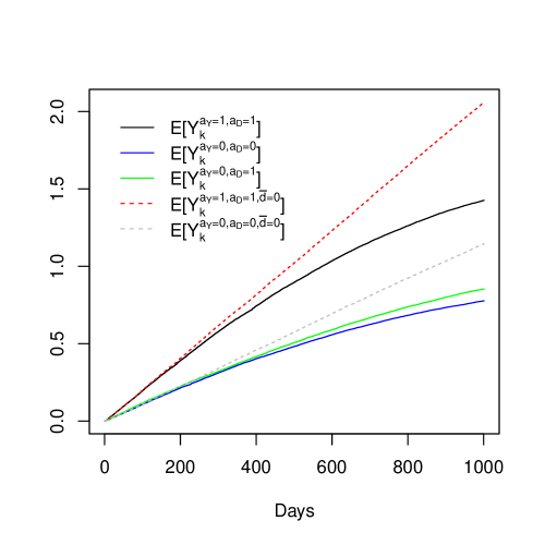
(a)

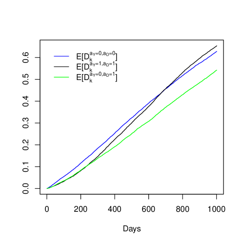
(b)

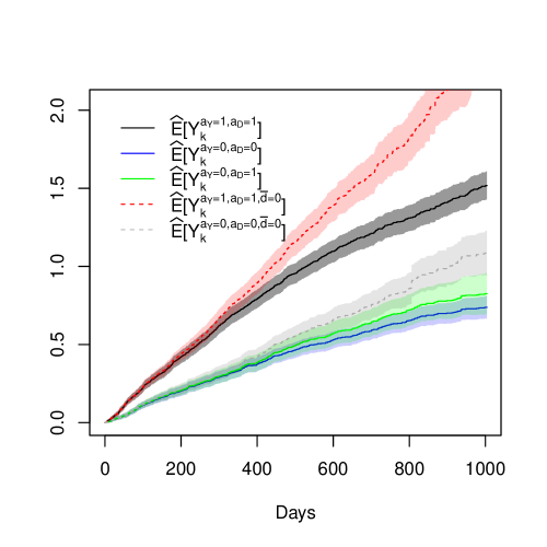
(c)

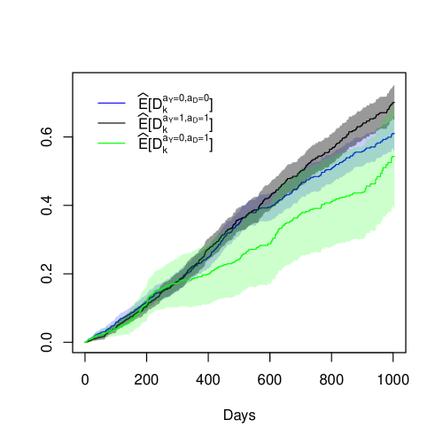
(d)

Figure 6. Different effects of treatment (dis)continuation of antihypertensives ($A_{Y}$) and aspirin ($A_{D}$) on recurrent syncope and survival are shown in (A) and (B), under a hypothetical data generating mechanism. The superscript $\overline{c}=0$, denoting an intervention to prevent loss to follow-up, has been suppressed in plot legends to reduce clutter. Estimates using the risk set estimator in Eq. 45 with a sample size of 1000 individuals in each treatment arm are shown in (C) and (D). 95% pointwise confidence intervals obtained from a bootstrap sample of 400 are indicated in the shaded regions. The width of the confidence interval for $\hat{E}[D_{k}^{a_{Y}=0,a_{D}=1}]$ reflects that the term $\theta^{D}$ is included for that estimand in Table 3, coming from the fact that $\mathcal{W}_{D}(a_{Y},a_{D})$ share its jump times with $N^{D}$.

By transforming the graphs in Fig. 5 to single world intervention graphs (Richardson and Robins, 2013b) corresponding to Figs. 2-4, it is straightforward to verify that the exchangeability (Eqs. 12-13, 19-20 and  24-25) and dismissible component conditions (Eqs. 27-30) are satisfied by the causal model. Because all positivity and consistency conditions also hold by construction in the data generating model, the total, controlled direct and separable effects are identified by the respective functionals given in Secs. 5.1-5.3.

Table 5. The left column includes the weights, the midddle column includes the hazards that define Eq. 47, and the right column includes the parametric hazard models that were used in the data analysis.

Weight	Hazards	Hazard models fitted
$\overline{\mathcal{W}}_{C,t}^{i}$	$\alpha_{t}^{i}dt$	$\beta_{t}^{0}+\beta_{t}^{A}A+\beta_{t}^{L_{0}}L_{0}+\beta_{t}^{L_{1}}L_{1}+\beta_{t}^{Y}Y_{t-}$
	$\alpha_{t}^{*,i}dt$	$0$
$\mathcal{W}_{C,t}^{i}$	$\alpha_{t}^{i}dt$	$\beta_{t}^{0}+\beta_{t}^{A}A+\beta_{t}^{L_{0}}L_{0}+\beta_{t}^{L_{1}}L_{1}+\beta_{t}^{Y}Y_{t-}$
	$\alpha_{t}^{*,i}dt$	$\beta_{t}^{0}+\beta_{t}^{A}A$
$\overline{\mathcal{W}}_{D,t}^{i}$	$\alpha_{t}^{i}dt$	$\beta_{0}^{D}+\beta_{A}^{D}A+\beta_{L_{0}}^{D}L_{0}+\beta_{L_{1}}^{D}L_{1}+\beta_{Y}^{D}Y_{t-}$
	$\alpha_{t}^{*,i}dt$	$0$
$\mathcal{W}_{D,t}^{i}$	$\alpha_{t}^{i}dt$	$\beta_{t}^{0}+\beta_{t}^{A}A+\beta_{t}^{L_{0}}L_{0}+\beta_{t}^{L_{1}}L_{1}+\beta_{t}^{Y}Y_{t-}$
	$\alpha_{t}^{*,i}dt$	$\beta_{t}^{0}+\beta_{t}^{A}A$
$\mathcal{W}_{D,t}^{i}(a_{Y},a_{D})$	$\alpha_{t}^{i}dt$	$\beta_{t}^{0}+\beta_{t}^{A}I(A=a_{Y})+\beta_{t}^{L_{0}}L_{0}+\beta_{t}^{L_{1}}L_{1}+\beta_{t}^{Y}Y_{t-}$
	$\alpha_{t}^{*,i}dt$	$\beta_{t}^{0}+\beta_{t}^{A}I(A=a_{D})+\beta_{t}^{L_{0}}L_{0}+\beta_{t}^{L_{1}}L_{1}+\beta_{t}^{Y}Y_{t-}$

7.1. Estimates

Figs. 6 (C) and (D) present estimates of $E[Y^{a,\overline{c}=0}]$ for $a=a_{Y}=a=D\in\{0,1\}$ and $E[Y^{a_{Y},a_{D},\overline{c}=0}]$ for $a_{Y}\neq a_{D}$ using the estimators described in Sec. 6 for 1000 simulated individuals in each of the treatment groups $A=0$ and $A=1$. It follows from the data-generating model defined in the beginning of Sec. 7 and Table 5 that the assumed hazard models are correctly specified (in the case of $\overline{\mathcal{W}}_{D},\mathcal{W}_{D}$, and $\mathcal{W}_{D}(a,a_{D})$). We could allow for a more involved data generating mechanism with time-varying coefficients. The assumed hazard models would still provide consistent estimates if the additive structure is correctly specified. Thus, an investigator can adapt the estimators in the supplementary R markdown file to other recurrent event problems. For the given sample size, the point estimates shown in Fig. 6 are unbiased (see the data-generating mechanism described in Sec. 7).

8. Discussion

We have used a counterfactual framework to formally define estimands for recurrent outcomes that differ in the way they treat competing events. The controlled direct effect is a contrast of counterfactual outcomes which implies that competing events are considered to be a form of censoring. The total effect captures all causal pathways between treatment and the recurrent event, and the separable effect quantifies contrasts in expected outcomes under independent prescription of treatment components.

Further, we have given formal conditions for identifying these effects, and demonstrated how to evaluate the identification conditions in causal graphs. This allowed us to formally describe how the causal estimands map to classical statistical estimands for recurrent events based on counting processes in the limit of fine discretizations of time.

In settings with competing events, it is often of interest to disentangle the effect on the recurrent event from the effect on the competing event. The controlled direct effect often fails to do so in a scientifically insightful way, because it is not clear which intervention, if any, eliminates the occurrence of the competing event. The interpretation of the direct effect is therefore unclear. The separable effect corresponds (by design) to a well-defined intervention in which we conceptually decompose the original treatment into components, which we then assign independently of each other. The practical relevance of the estimand relies on the plausibility of modified treatments. The process of conceptualizing modified treatments can motivate future treatment development and sharpen research questions about mechanisms (Robins and Richardson, 2011; Robins et al., 2020; Stensrud et al., 2020b).

Stronger assumptions are needed to identify the (controlled) direct effect and separable effects compared to the total effect. For example, these estimands require the investigator to measure common causes of the recurrent event and failure time, even in an ideal randomized trial such as in Sec. 2. The need for stronger assumptions is far from unique to our setting, and it is analogous to the task of identifying per-protocol effects in settings with imperfect adherence and mediation effects.

The use of a formal (counterfactual) framework to define causal effects elucidates analytic choices regarding treatment recommendations. The formal causal framework makes it possible to define effects with respect to explicit interventions, and to explicitly state the conditions in which such effects can be identified from observed data. This also makes it possible to transparently assess the strength and validity of the identifying assumptions in practice.

Appendix A Isolation conditions

Following Stensrud et al. (2021), we define the $A_{Y}$ separable effect on $Y_{k}$ as

(49) $$E[Y_{k}^{a_{Y}=1,a_{D}}]-E[Y_{k}^{a_{Y}=0,a_{D}}]\leavevmode\nobreak\ .$$

Likewise, we define the $A_{D}$ separable effect on $Y_{k}$ as

(50) $$E[Y_{k}^{a_{Y},a_{D}=1}]-E[Y_{k}^{a_{Y},a_{D}=0}]\leavevmode\nobreak\ .$$

Next, following Stensrud et al. (2021), we define two isolation conditions:

Definition 2 (Strong $A_{Y}$ partial isolation).

A treatment decomposition satisfies strong $A_{Y}$ partial isolation if

(51) There are no causal paths from $$A_{Y} D_{k} k\in\{0,\cdots,k+1\}$$ to for all  .

Definition 3 ($A_{D}$ partial isolation).

A treatment decomposition satisfies $A_{D}$ partial isolation if

The causal paths from $$A_{D} Y_{k+1} k=0,\dots,K$$ to , are directed

(52) paths intersected by $$D_{j+1} j\in\{0,\cdots,K\}$$,  .

Under strong $A_{Y}$ partial isolation, the $A_{Y}$ separable effects only capture direct effects of $A_{Y}$ on $Y_{k}$, i.e. only pathways from $A_{Y}$ to $Y_{k}$ not intersected by $D$. Under $A_{D}$ partial isolation, the $A_{D}$ separable effects only capture indirect effects of $A_{D}$ on $Y_{k}$, that is only pathways from $A_{D}$ to $Y_{k}$ that are intersected by $D$.

If a treatment decomposition satisfies both Eq. 51 and 52, it is said to satisfy full isolation. Under full isolation, Eqs. 49-50 are the separable direct and indirect effects on $Y_{k}$ respectively. In this case, Eq. 49 captures all pathways from $A$ to $Y_{k}$ not intersected by $D$, and Eq. 50 captures all pathways from $A$ to $Y_{k}$ intersected by $D$.

Appendix B Proof of identification results

B.1. Total effect

Assume the following identification conditions hold:

Exchangeability

$$\overline{Y}_{K+1}^{a,\overline{c}=0} \mathchoice{\mathrel{\hbox to0.0pt{$\displaystyle\perp$\hss}\mkern 2.0mu{\displaystyle\perp}}}{\mathrel{\hbox to0.0pt{$\textstyle\perp$\hss}\mkern 2.0mu{\textstyle\perp}}}{\mathrel{\hbox to0.0pt{$\scriptstyle\perp$\hss}\mkern 2.0mu{\scriptstyle\perp}}}{\mathrel{\hbox to0.0pt{$\scriptscriptstyle\perp$\hss}\mkern 2.0mu{\scriptscriptstyle\perp}}}A|L_{0}\leavevmode\nobreak\ ,$$

$$\underline{Y}_{k+1}^{a,\overline{c}=0} \mathchoice{\mathrel{\hbox to0.0pt{$\displaystyle\perp$\hss}\mkern 2.0mu{\displaystyle\perp}}}{\mathrel{\hbox to0.0pt{$\textstyle\perp$\hss}\mkern 2.0mu{\textstyle\perp}}}{\mathrel{\hbox to0.0pt{$\scriptstyle\perp$\hss}\mkern 2.0mu{\scriptstyle\perp}}}{\mathrel{\hbox to0.0pt{$\scriptscriptstyle\perp$\hss}\mkern 2.0mu{\scriptscriptstyle\perp}}}C_{k+1}^{a,\overline{c}=0}|\overline{L}_{k}^{a,\overline{c}=0},\overline{Y}_{k}^{a,\overline{c}=0},\overline{D}_{k}^{a,\overline{c}=0},\overline{C}_{k}^{a,\overline{c}=0},A\leavevmode\nobreak\ .$$

Positivity

$$P(L_{0}=l_{0})>0\implies P(A=a\mid L_{0}=l_{0})>0\leavevmode\nobreak\ ,$$

$$f_{A,\overline{L}_{k},\overline{D}_{k},\overline{C}_{k},\overline{Y}_{k}}(a,\overline{l}_{k},0,0,\overline{y}_{k})>0$$

$$\quad\implies P(C_{k+1}=0\mid A=a,\overline{L}_{k}=\overline{l}_{k},\overline{D}_{k}=0,\overline{C}_{k}=0,\overline{Y}_{k}=\overline{y}_{k})>0\leavevmode\nobreak\ .$$

Consistency

If $$A=a \overline{C}_{k+1}=0$$ and ,

$$\text{then $\overline{L}_{k+1}=\overline{L}_{k+1}^{a,\overline{c}=0},\overline{D}_{k+1}=\overline{D}_{k+1}^{a,\overline{c}=0},\overline{Y}_{k+1}=\overline{Y}_{k+1}^{a,\overline{c}=0}$},\overline{C}_{k+1}=\overline{C}_{k+1}^{a,\overline{c}=0}\leavevmode\nobreak\ .$$

Next, we use the identification conditions and the law of total probability (LOTP) to add variables sequentially to the conditioning set in temporal order. We have that $P(\Delta Y_{k}^{a,\overline{c}=0}=\Delta y_{k})$ is given by

$$\sum_{l_{0}}P(\Delta Y_{k}^{a,\overline{c}=0}=\Delta y_{k}\mid L_{0}=l_{0})P(L_{0}=l_{0})$$

$$\stackrel{{\scriptstyle\overline{Y}_{K+1}^{a,\overline{c}=0}\mathchoice{\mathrel{\hbox to0.0pt{$\displaystyle\perp$\hss}\mkern 2.0mu{\displaystyle\perp}}}{\mathrel{\hbox to0.0pt{$\textstyle\perp$\hss}\mkern 2.0mu{\textstyle\perp}}}{\mathrel{\hbox to0.0pt{$\scriptstyle\perp$\hss}\mkern 2.0mu{\scriptstyle\perp}}}{\mathrel{\hbox to0.0pt{$\scriptscriptstyle\perp$\hss}\mkern 2.0mu{\scriptscriptstyle\perp}}}A\mid L_{0}}}{{=}}\sum_{l_{0}}P(\Delta Y_{k}^{a,\overline{c}=0}=\Delta y_{k}\mid A=a,L_{0}=l_{0})P(L_{0}=l_{0})$$

$$\stackrel{{\scriptstyle\underline{Y}_{0}^{a,\overline{c}=0}\mathchoice{\mathrel{\hbox to0.0pt{$\displaystyle\perp$\hss}\mkern 2.0mu{\displaystyle\perp}}}{\mathrel{\hbox to0.0pt{$\textstyle\perp$\hss}\mkern 2.0mu{\textstyle\perp}}}{\mathrel{\hbox to0.0pt{$\scriptstyle\perp$\hss}\mkern 2.0mu{\scriptstyle\perp}}}{\mathrel{\hbox to0.0pt{$\scriptscriptstyle\perp$\hss}\mkern 2.0mu{\scriptscriptstyle\perp}}}C_{0}^{a}\mid A,L_{0}}}{{=}}\sum_{l_{0}}P(\Delta Y_{k}^{a,\overline{c}=0}=\Delta y_{k}\mid C_{0}^{a}=0,A=a,L_{0}=l_{0})P(L_{0}=l_{0})$$

$$\stackrel{{\scriptstyle\text{LOTP}}}{{=}}\sum_{d_{0}}\sum_{l_{0}}P(\Delta Y_{k}^{a,\overline{c}=0}=\Delta y_{k}\mid D_{0}^{a,c_{0}=0}=0,C_{0}^{a}=0,A=a,L_{0}=l_{0})$$

$$\qquad\times P(D_{0}^{a,c_{0}=0}=0\mid C_{0}^{a}=0,A=a,L_{0}=l_{0})P(L_{0}=l_{0})$$

$$\stackrel{{\scriptstyle\text{LOTP}}}{{=}}\sum_{\Delta y_{0}}\sum_{d_{0}}\sum_{l_{0}}P(\Delta Y_{k}^{a,c_{0}=0}=\Delta y_{k}\mid\Delta Y_{0}^{a,\overline{c}=0}=\Delta y_{0},D_{0}^{a,c_{0}=0}=0,C_{0}^{a}=0,A=a,L_{0}=l_{0})$$

$$\qquad P(\Delta Y_{0}^{a,c_{0}=0}=\Delta y_{0}\mid D_{0}^{a,c_{0}=0}=0,C_{0}^{a}=0,A=a,L_{0}=l_{0})$$

$$\qquad\times P(D_{0}^{a,c_{0}=0}=0\mid C_{0}^{a}=0,A=a,L_{0}=l_{0})P(L_{0}=l_{0})\leavevmode\nobreak\ .$$

The conditional independence relation in the third line follows because $C_{0}\equiv 0$ deterministically. Iterating this procedures for time indices $k^{\prime}\in\{1,\dots,k\}$ gives

$$P(\Delta Y_{k}^{a,\overline{c}=0}=\Delta y_{k})$$

$$=\sum_{\Delta\overline{y}_{k-1}}\sum_{\overline{d}_{k}}\sum_{\overline{l}_{k-1}}\prod_{j=0}^{k}$$

$$\qquad P(\Delta Y_{j}^{a,\overline{c}=0}=\Delta y_{j}\mid\overline{D}_{j}^{a,\overline{c}=0}=\overline{d}_{j},\overline{C}_{j}^{a,\overline{c}=0}=0,\overline{L}_{j-1}^{a,\overline{c}=0}=\overline{l}_{j-1},\Delta\overline{Y}_{j-1}^{a,\overline{c}=0}=\Delta\overline{y}_{j-1},A=a)$$

$$\qquad\times P(D_{j}^{a,\overline{c}=0}=d_{j}\mid\overline{C}_{j}^{a,\overline{c}=0}=0,\overline{L}_{j-1}^{a,\overline{c}=0}=\overline{l}_{j-1},\Delta\overline{Y}_{j-1}^{a,\overline{c}=0}=\Delta\overline{y}_{j-1},\overline{D}_{j-1}^{a,\overline{c}=0}=\overline{d}_{j-1},A=a)$$

$$\qquad\times P(L_{j-1}^{a,\overline{c}=0}=l_{j-1}\mid\Delta\overline{Y}_{j-1}^{a,\overline{c}=0}=\Delta\overline{y}_{j-1},\overline{D}_{j-1}^{a,\overline{c}=0}=\overline{d}_{j-1},\overline{C}_{j-1}^{a,\overline{c}=0}=0,\overline{L}_{j-2}^{a,\overline{c}=0}=\overline{l}_{j-2},A=a)\leavevmode\nobreak\ .$$

Positivity ensures that the conditioning sets on RHS have a non-zero probability. Finally, by consistency we have that

$$P( \Delta Y_{k}^{a,\overline{c}=0}=\Delta y_{k})$$

$$=\sum_{\Delta\overline{y}_{k-1}}\sum_{\overline{d}_{k}}\sum_{\overline{l}_{k-1}}\prod_{j=0}^{k}$$

$$\qquad P(\Delta Y_{j}=\Delta y_{j}\mid\overline{D}_{j}=\overline{d}_{j},\overline{C}_{j}=0,\overline{L}_{j-1}=\overline{l}_{j-1},\Delta\overline{Y}_{j-1}=\Delta\overline{y}_{j-1},A=a)$$

$$\qquad\times P(D_{j}=d_{j}\mid\overline{C}_{j}=0,\overline{L}_{j-1}=\overline{l}_{j-1},\Delta\overline{Y}_{j-1}=\Delta\overline{y}_{j-1},\overline{D}_{j-1}=\overline{d}_{j-1},A=a)$$

$$\qquad\times P(L_{j-1}=l_{j-1}\mid\Delta\overline{Y}_{j-1}=\Delta\overline{y}_{j-1},\overline{D}_{j-1}=\overline{d}_{j-1},\overline{C}_{j-1}=0,\overline{L}_{j-2}=\overline{l}_{j-2},A=a)\leavevmode\nobreak\ .$$

Next, we derive Eq. 18. By the presence of the indicator functions in Eq. 18 and by consistency (Eq. 16) we have that

$$E\left[\frac{I(A=a)I(C_{i}=0)\Delta Y_{i}}{\pi_{A}(A)\prod_{j=0}^{i}\pi_{C_{j}}(C_{j})}\right]$$

$$= E\left[\frac{I(A=a)I(C_{i}=0)\Delta Y_{i}^{a,\overline{c}=0}}{\pi_{A}(A)\prod_{j=0}^{i}\pi_{C_{j}}(C_{j})}\right]$$

$$= E\left[\frac{I(A=a)I(C_{i}^{a,\overline{c}=0}=0)\Delta Y_{i}^{a,\overline{c}=0}}{P(A=a\mid L_{0})\prod_{j=0}^{i}P(C_{j}^{a,\overline{c}=0}=0\mid\overline{L}_{j-1}^{a,\overline{c}=0},\overline{Y}_{j-1}^{a,\overline{c}=0},\overline{D}_{j-1}^{a,\overline{c}=0},\overline{C}_{j-1}^{a,\overline{c}=0},A)}\right]\leavevmode\nobreak\ .$$

Next, using the law of total expectation, the above is equal to

$$E\bigg{[}E\bigg{[}\frac{I(A=a)I(C_{i}^{a,\overline{c}=0}=0)\Delta Y_{i}^{a,\overline{c}=0}}{P(A=a\mid L_{0})\prod_{j=0}^{i}P(C_{j}^{a,\overline{c}=0}=0\mid\overline{L}_{j-1}^{a,\overline{c}=0},\overline{Y}_{j-1}^{a,\overline{c}=0},\overline{D}_{j-1}^{a,\overline{c}=0},\overline{C}_{j-1}^{a,\overline{c}=0},A)}$$

$$\qquad\qquad\qquad\leavevmode\nobreak\ \bigg{|}\leavevmode\nobreak\ \overline{Y}_{i}^{a,\overline{c}=0},\overline{L}_{i-1}^{a,\overline{c}=0},\overline{D}_{i-1}^{a,\overline{c}=0},\overline{C}_{i-1}^{a,\overline{c}=0},A\bigg{]}\bigg{]}$$

$$= E\bigg{[}\frac{I(A=a)I(C_{i-1}^{a,\overline{c}=0}=0)\Delta Y_{i}^{a,\overline{c}=0}}{P(A=a\mid L_{0})\prod_{j=0}^{i-1}P(C_{j}^{a,\overline{c}=0}=0\mid\overline{L}_{j-1}^{a,\overline{c}=0},\overline{Y}_{j-1}^{a,\overline{c}=0},\overline{D}_{j-1}^{a,\overline{c}=0},\overline{C}_{j-1}^{a,\overline{c}=0},A)}$$

$$\qquad\times\underbrace{\frac{E[I(C_{i}^{a,\overline{c}=0}=0)\mid\overline{Y}_{i}^{a,\overline{c}=0},\overline{L}_{i-1}^{a,\overline{c}=0},\overline{D}_{i-1}^{a,\overline{c}=0},\overline{C}_{i-1}^{a,\overline{c}=0},A]}{P(C_{i}^{a,\overline{c}=0}=0\mid\overline{L}_{i-1}^{a,\overline{c}=0},\overline{Y}_{i-1}^{a,\overline{c}=0},\overline{D}_{i-1}^{a,\overline{c}=0},\overline{C}_{i-1}^{a,\overline{c}=0},A)}}_{(\star)}\bigg{]}\bigg{]}\leavevmode\nobreak\ .$$

The numerator and denominator of the fraction in the final line, indicated by $(\star)$, differ only by the time index of $\overline{Y}^{a,\overline{c}=0}$ in the conditioning set. Using the fact that

$$Y_{i}^{a,\overline{c}=0}\mathchoice{\mathrel{\hbox to0.0pt{$\displaystyle\perp$\hss}\mkern 2.0mu{\displaystyle\perp}}}{\mathrel{\hbox to0.0pt{$\textstyle\perp$\hss}\mkern 2.0mu{\textstyle\perp}}}{\mathrel{\hbox to0.0pt{$\scriptstyle\perp$\hss}\mkern 2.0mu{\scriptstyle\perp}}}{\mathrel{\hbox to0.0pt{$\scriptscriptstyle\perp$\hss}\mkern 2.0mu{\scriptscriptstyle\perp}}}I(C_{i}^{a,\overline{c}=0}=0)\mid Y_{i-1}^{a,\overline{c}=0},L_{i-1}^{a,\overline{c}=0},D_{i-1}^{a,\overline{c}=0},C_{i-1}^{a,\overline{c}=0}=0,A=a\leavevmode\nobreak\ ,$$

(which follows from Eq. 13) we have that $(\star)=1$, and thus by consistency (Eq. 16),

$$E\left[\frac{I(A=a)I(C_{i}=0)\Delta Y_{i}^{a,\overline{c}=0}}{\pi_{A}(A)\prod_{j=0}^{i}\pi_{C_{j}}(C_{j})}\right]=E\left[\frac{I(A=a)I(C_{i-1}=0)\Delta Y_{i}^{a,\overline{c}=0}}{\pi_{A}(A)\prod_{j=0}^{i-1}\pi_{C_{j}}(C_{j})}\right]\leavevmode\nobreak\ .$$

Iterating this procedure from $j=i-1$ to $j=0$ gives

$$E\left[\frac{I(A=a)I(C_{i}=0)\Delta Y_{i}^{a,\overline{c}=0}}{\pi_{A}(A)\prod_{j=0}^{i}\pi_{C_{j}}(C_{j})}\right]=E\left[\frac{I(A=a)\Delta Y_{i}^{a,\overline{c}=0}}{\pi_{A}(A)}\right]\leavevmode\nobreak\ .$$

Using the law of total expectation again, RHS is equal to

$$E\left[E\left[\frac{\Delta Y_{i}^{a,\overline{c}=0}}{P(A=a\mid L_{0})}\cdot I(A=a)\leavevmode\nobreak\ \bigg{|}\leavevmode\nobreak\ \Delta Y_{i}^{a,\overline{c}=0},L_{0}\right]\right]$$

$$= E\left[\frac{\Delta Y_{i}^{a,\overline{c}=0}}{P(A=a\mid L_{0})}\cdot E\left[I(A=a)\mid\Delta Y_{i}^{a,\overline{c}=0},L_{0}\right]\right]$$

$$\stackrel{{\scriptstyle\Delta Y_{i}^{a,\overline{c}=0}\mathchoice{\mathrel{\hbox to0.0pt{$\displaystyle\perp$\hss}\mkern 2.0mu{\displaystyle\perp}}}{\mathrel{\hbox to0.0pt{$\textstyle\perp$\hss}\mkern 2.0mu{\textstyle\perp}}}{\mathrel{\hbox to0.0pt{$\scriptstyle\perp$\hss}\mkern 2.0mu{\scriptstyle\perp}}}{\mathrel{\hbox to0.0pt{$\scriptscriptstyle\perp$\hss}\mkern 2.0mu{\scriptscriptstyle\perp}}}I(A=a)\mid L_{0}}}{{=}} E\left[\Delta Y_{i}^{a,\overline{c}=0}\cdot\frac{E[I(A=a)\mid L_{0}]}{P(A=a\mid L_{0})}\right]$$

$$= E[\Delta Y_{i}^{a,\overline{c}=0}]\leavevmode\nobreak\ .$$

Another IPW representation also exists. We have that

$$E\bigg{[}\frac{I(A=a)I(C_{i}=0)}{\pi_{A}(A)\prod_{j=0}^{i}\pi_{C_{j}}(C_{j})}\bigg{]}$$

$$= E\bigg{[}E\bigg{[}\frac{I(A=a)I(C_{i-1}=0)}{\pi_{A}(A)\prod_{j=0}^{i-1}\pi_{C_{j}}(C_{j})}\cdot\frac{I(C_{i}=0)}{P(C_{i}=0\mid\overline{L}_{i-1},\overline{Y}_{i-1},\overline{D}_{i-1},\overline{C}_{i-1},A=a)}$$

$$\qquad\qquad\qquad\leavevmode\nobreak\ \bigg{|}\leavevmode\nobreak\ \overline{L}_{i-1},\overline{Y}_{i-1},\overline{D}_{i-1},\overline{C}_{i-1},A=a\bigg{]}\bigg{]}$$

$$= E\bigg{[}\frac{I(A=a)I(C_{i-1}=0)}{\pi_{A}(A)\prod_{j=0}^{i-1}\pi_{C_{j}}(C_{j})}\cdot\frac{E[I(C_{i}=0)\mid\overline{L}_{i-1},\overline{Y}_{i-1},\overline{D}_{i-1},\overline{C}_{i-1},A=a]}{P(C_{i}=0\mid\overline{L}_{i-1},\overline{Y}_{i-1},\overline{D}_{i-1},\overline{C}_{i-1},A=a)}\bigg{]}$$

$$= E\bigg{[}\frac{I(A=a)I(C_{i-1}=0)}{\pi_{A}(A)\prod_{j=0}^{i-1}\pi_{C_{j}}(C_{j})}\bigg{]}\leavevmode\nobreak\ .$$

Arguing iteratively from $j=i-1$ to $j=0$, the RHS is equal to

$$E\left[\frac{I(A=a)}{P(A=a\mid L_{0})}\right] =E\left[E\left[\frac{I(A=a)}{P(A=a\mid L_{0})}\leavevmode\nobreak\ \bigg{|}\leavevmode\nobreak\ L_{0}\right]\right]$$

$$=E\left[\frac{E[I(A=a)\mid L_{0}]}{P(A=a\mid L_{0})}\right]$$

$$=1\leavevmode\nobreak\ .$$

Putting everything together, we have that

(53) $$E[Y_{k}^{a,\overline{c}=0}] =\sum_{i=1}^{k}\frac{E\bigg{[}\frac{I(A=a)I(C_{i}=0)}{\pi_{A}(A)\prod_{j=1}^{i}\pi_{C_{j}}(C_{j})}\cdot\Delta Y_{i}\bigg{]}}{E\bigg{[}\frac{I(A=a)I(C_{i}=0)}{\pi_{A}(A)\prod_{j=1}^{i}\pi_{C_{j}}(C_{j})}\bigg{]}}\leavevmode\nobreak\ .$$

To conclude, we remark that the exchangeability conditions Eqs. 12-13 and identification formulas Eq. LABEL:eq:g-formula_total_effect-18 follow directly from a general identification result, Theorem 31 of  Richardson and Robins (2013b), by choosing outcome $Y^{\ast}_{k}\equiv(Y_{k},D_{K+1})$, intervention set $\overline{A}^{\ast}_{k}\equiv(A,C_{k})$ for $k\in\{0,\dots,K+1\}$ and time-varying covariates $\overline{L}^{\ast}_{k}\equiv(\overline{L}_{k},L)$ for $k\in\{0,\dots,K\}$.

B.1.1. Limit of fine discretizations

We begin by noting that $\Delta Y_{k}$ in Eq. 53 can only be non-zero if the individual has not experienced the competing event by beginning of the time interval $k-1$. Therefore,

$$E[\Delta Y_{i}^{a,\overline{c}=0}] =E\left[\frac{I(A=a)I(\overline{C}_{i}=0)I(\overline{D}_{i-1}=0)\Delta Y_{i}}{\pi_{A}\prod_{j=0}^{i}\pi_{C_{j}}(C_{j})}\right]$$

$$=P(\overline{C}_{i}=0,\overline{D}_{i-1}=0,A=a)$$

$$\qquad\times E\left[\frac{\Delta Y_{i}}{\pi_{A}\prod_{j=0}^{i}\pi_{C_{k}}(C_{k})}\leavevmode\nobreak\ \bigg{|}\leavevmode\nobreak\ A=a,C_{i}=0,D_{i-1}=0\right]\leavevmode\nobreak\ ,$$

where we have used the laws of probability in the second line. Using Bayes’ law sequentially, we have that

$$P(\overline{C}_{i}=0,\overline{D}_{i-1}=0,A=a) =\prod_{j=1}^{i-1}\bigg{[}P(D_{j}=0\mid C_{j}=0,D_{j-1}=0,A=a)\bigg{]}$$

$$\quad\times\prod_{n=1}^{i}\bigg{[}P(C_{n}=0\mid D_{n-1}=0,C_{n-1}=0,A=a)\bigg{]}P(A=a)\leavevmode\nobreak\ .$$

To proceed, we define modified intensities of the recurrent event process

$$\Delta\Uplambda_{i}^{C} =P(C_{i}=1\mid\overline{D}_{i-1},\overline{C}_{i-1},A)$$

$$\Delta\Uplambda_{i}^{C\mid\mathcal{F}} =P(C_{i}=1\mid\overline{L}_{i-1},\overline{Y}_{i-1},\overline{D}_{i-1},\overline{C}_{i-1},A)\leavevmode\nobreak\ .$$

Next, let $\pi(\bullet)=P(A=\bullet)$ and consider the stabilized weights

$$W_{A} =\frac{\pi(A)}{\pi_{A}(A)}\leavevmode\nobreak\ ,$$

$$W_{C,i} =\frac{\prod_{j=1}^{i}[1-\Delta\Uplambda_{j}^{C}]}{\prod_{k=1}^{i}\left[1-\Delta\Uplambda_{k}^{C\mid\mathcal{F}}\right]}\leavevmode\nobreak\ .$$

The weight $W_{C,i}$ is a ratio of Kaplan-Meier survival terms with the respect to the censoring event. Let us also define the hazard of the competing event by

$$\Delta A^{D}_{i}(a)=P(D_{i}=1\mid C_{i}=0,D_{i-1}=0,A=a)\leavevmode\nobreak\ .$$

Putting everything together, we have that

(54) $$E[Y_{k}^{a,\overline{c}=0}]=\sum_{i=1}^{k}\prod_{j=1}^{i-1}[1-\Delta A_{j}^{D}(a)]\cdot E[W_{A}W_{C,i}\Delta Y_{i}\mid C_{i}=0,D_{i-1}=0,A=a]\leavevmode\nobreak\ .$$

Eq. 54 enables us to establish a correspondence with estimands in the counting process literature, as discussed in Sec. 5.4.2, and also motivates estimators that we described in Sec. 6. The product term in Eq. 54 is a survival term with respect to the competing event, and the expectation is over weighted increments of the recurrent syncope. In the limit of fine discretization of time, Eq. 54 converges to

$$\int_{0}^{t_{k}}\prodi_{s<u}[1-dA_{s}^{D}(a)]\cdot E[W_{A}\mathcal{W}_{C,u-}dN_{u}\mid C\geq u,T^{D}\geq u,A=a]\leavevmode\nobreak\ .$$

B.1.2. Competing event

In order to identify $E[D_{k}^{a,\overline{c}=0}]$ from the observed data, we require the following two exchangeability assumptions instead of Eqs. 12 and 13

(55) $$\overline{D}_{K+1}^{a,\overline{c}=0} \mathchoice{\mathrel{\hbox to0.0pt{$\displaystyle\perp$\hss}\mkern 2.0mu{\displaystyle\perp}}}{\mathrel{\hbox to0.0pt{$\textstyle\perp$\hss}\mkern 2.0mu{\textstyle\perp}}}{\mathrel{\hbox to0.0pt{$\scriptstyle\perp$\hss}\mkern 2.0mu{\scriptstyle\perp}}}{\mathrel{\hbox to0.0pt{$\scriptscriptstyle\perp$\hss}\mkern 2.0mu{\scriptscriptstyle\perp}}}A|L_{0}\leavevmode\nobreak\ ,$$

(56) $$\underline{D}_{k+1}^{a,\overline{c}=0} \mathchoice{\mathrel{\hbox to0.0pt{$\displaystyle\perp$\hss}\mkern 2.0mu{\displaystyle\perp}}}{\mathrel{\hbox to0.0pt{$\textstyle\perp$\hss}\mkern 2.0mu{\textstyle\perp}}}{\mathrel{\hbox to0.0pt{$\scriptstyle\perp$\hss}\mkern 2.0mu{\scriptstyle\perp}}}{\mathrel{\hbox to0.0pt{$\scriptscriptstyle\perp$\hss}\mkern 2.0mu{\scriptscriptstyle\perp}}}C_{k+1}^{a,\overline{c}=0}|\overline{L}_{k}^{a,\overline{c}=0},\overline{Y}_{k}^{a,\overline{c}=0},\overline{D}_{k}^{a,\overline{c}=0},\overline{C}_{k}^{a,\overline{c}=0},A\leavevmode\nobreak\ .$$

Using analogous arguments as for the recurrent event $Y$, identification of $E[D_{k}^{a,\overline{c}=0}]$ is achieved under Eqs. 55-56 and Eqs. 14-16 by

(57) $$E[D_{k}^{a,\overline{c}=0}]=\sum_{i=1}^{k}\prod_{j=1}^{i-1}[1-\Delta A_{j}^{D}(a)]\cdot E[W_{A}W_{C,i}\Delta D_{i}\mid C_{i}=0,D_{i-1}=0,A=a]\leavevmode\nobreak\ .$$

Likewise, in the limit of fine discretizations of time, the cumulative incidence of the competing event is given by

(58) $$\int_{0}^{t_{k}}\prodi_{s<u}[1-dA_{s}^{D}(a)]\cdot E[W_{A}\mathcal{W}_{C,u-}dI(T^{D}\geq u)\mid C\geq u,T^{D}\geq u,A=a]\leavevmode\nobreak\ .$$

When treatment $A$ is randomly assigned and Eq. 87 holds with $L(t)=N^{c}(t)=\emptyset$ (which is the usual independent censoring condition in survival analysis without any covariates (Aalen et al., 2008)), then $W_{A}=\mathcal{W}_{C,t}=1$ and Eq. 58 reduces to

$$\int_{0}^{t_{k}}\prodi_{u\leq t}[1-dA^{D}_{u}(a)]dA^{D}_{u}(a)\leavevmode\nobreak\ .$$

This demonstrates sufficient conditions under which the discrete-time identification formula Eq. 29 in Young et al. (2020) converges to the usual representation of the cumulative incidence function in survival analysis.

B.2. Controlled direct effect

The identification conditions and identification formulas for direct effect are a special case of the identification results for total effect, redefining the censoring indicator as $\max(C_{i},D_{i})$ (i.e. the first occurrence of the competing event and loss to follow-up), and re-defining the competing event as an event that almost surely does not occur. This gives us

(59) $$E[\Delta Y_{i}^{a,\overline{c}=\overline{d}=0}] =E\bigg{[}\frac{I(A=a)I(C_{i}=0)I(D_{i}=0)}{\pi_{A}(A)\prod_{j=1}^{i}\pi_{C_{j}}(C_{j})\pi_{D_{j}}(D_{j})}\cdot\Delta Y_{i}\bigg{]}\leavevmode\nobreak\ ,$$

Next, we define

$$\Delta\Uplambda_{j}^{D}(\bullet)=P(D_{j}=1\mid\overline{C}_{j},\overline{D}_{j-1},A=\bullet)\leavevmode\nobreak\ ,$$

$$\Delta\Uplambda_{j}^{D\mid\mathcal{F}}(\bullet)=P(D_{j}=1\mid\overline{C}_{j},\overline{L}_{j-1},\overline{Y}_{j-1},\overline{D}_{j-1},A=\bullet)$$

to be modified intensities of the competing event process. This allows us to re-write Eq. 59 as

(60) $$E[Y_{k}^{a,\overline{c}=\overline{d}=0}]=\sum_{i=1}^{k}E\left[W_{A}W_{C,i}W_{D,i}\Delta Y_{i}\leavevmode\nobreak\ \bigg{|}\leavevmode\nobreak\ C_{i}=0,D_{i-1}=0,A=a\right]\leavevmode\nobreak\ ,$$

where

(61) $$W_{D,i} =\frac{\prod_{j=1}^{i}[1-\Delta\Uplambda_{j}^{D}]}{\prod_{k=1}^{i}[1-\Delta\Uplambda_{k}^{D\mid\mathcal{F}}]}\leavevmode\nobreak\ .$$

Under randomization of $A$ and under the strong independent censoring assumption (Eq. 40), $W_{A}=W_{C,i}=W_{D,i}=1$ and thus Eq. 60 converges to

$$\int_{0}^{t_{k}}E\left[dN_{u}\mid T^{D}\geq u,C\geq u,A=a\right]\leavevmode\nobreak\ .$$

in the limit of fine discretizations of time.

B.3. Separable effects

We begin by assuming the modified treatment assumption (Eq. 4) and the identification conditions

Exchangeability

$$(\overline{Y}_{K+1}^{a,\overline{c}=0},\overline{D}_{K+1}^{a,\overline{c}=0},\overline{L}_{K+1}^{a,\overline{c}=0})\mathchoice{\mathrel{\hbox to0.0pt{$\displaystyle\perp$\hss}\mkern 2.0mu{\displaystyle\perp}}}{\mathrel{\hbox to0.0pt{$\textstyle\perp$\hss}\mkern 2.0mu{\textstyle\perp}}}{\mathrel{\hbox to0.0pt{$\scriptstyle\perp$\hss}\mkern 2.0mu{\scriptstyle\perp}}}{\mathrel{\hbox to0.0pt{$\scriptscriptstyle\perp$\hss}\mkern 2.0mu{\scriptscriptstyle\perp}}}A\mid L_{0}\leavevmode\nobreak\ ,$$

$$(\underline{Y}_{k+1}^{a,\overline{c}=0},\underline{D}_{k+1}^{a,\overline{c}=0},\underline{L}_{k+1}^{a,\overline{c}=0})\mathchoice{\mathrel{\hbox to0.0pt{$\displaystyle\perp$\hss}\mkern 2.0mu{\displaystyle\perp}}}{\mathrel{\hbox to0.0pt{$\textstyle\perp$\hss}\mkern 2.0mu{\textstyle\perp}}}{\mathrel{\hbox to0.0pt{$\scriptstyle\perp$\hss}\mkern 2.0mu{\scriptstyle\perp}}}{\mathrel{\hbox to0.0pt{$\scriptscriptstyle\perp$\hss}\mkern 2.0mu{\scriptscriptstyle\perp}}}C_{k+1}^{a,\overline{c}=0}\mid\overline{Y}_{k}^{a,\overline{c}=0},\overline{D}^{a,\overline{c}=0}_{k},\overline{C}_{k}^{a,\overline{c}=0},\overline{L}_{k}^{a,\overline{c}=0},A\leavevmode\nobreak\ .$$

Positivity

$$P(L_{0}=l_{0})>0$$

(62) $$\quad\implies P(A=a\mid L_{0}=l_{0})>0\leavevmode\nobreak\ ,$$

$$f_{\overline{L}_{k},\overline{D}_{k+1},C_{k+1},Y_{k}}(\overline{l}_{k},0,0,\overline{y}_{k})>0\implies$$

(63) $$\quad P(A=a\mid\overline{D}_{k+1}=0,C_{k+1}=0,\overline{Y}_{k}=\overline{y}_{k},\overline{L}_{k}=\overline{l}_{k})>0$$

$$f_{A,\overline{L}_{k},\overline{D}_{k},\overline{C}_{k},\overline{Y}_{k}}(a,\overline{l}_{k},0,0,\overline{y}_{k})>0$$

(64) $$\quad\implies P(C_{k+1}=0\mid\overline{L}_{k}=\overline{l}_{k},\overline{D}_{k}=0,\overline{C}_{k}=0,\overline{Y}_{k}=\overline{y}_{k})\leavevmode\nobreak\ .$$

for all $a\in\{0,1\}$, $k\in\{0,\dots,K+1\}$.

Consistency

If $$A=a \overline{C}_{k+1}=0$$ and ,

(65) $$\text{then $\overline{L}_{k+1}=\overline{L}_{k+1}^{a,\overline{c}=0},\overline{D}_{k+1}=\overline{D}_{k+1}^{a,\overline{c}=0},\overline{Y}_{k+1}=\overline{Y}_{k+1}^{a,\overline{c}=0}$}\leavevmode\nobreak\ .$$

Consider the setting in which we conduct a four armed trial in which the $A_{Y}$ and $A_{D}$ are randomly assigned, independently of each other. We require the following dismissible component conditions to hold in the four armed trial

$$Y_{k+1}^{\overline{c}=0}\mathchoice{\mathrel{\hbox to0.0pt{$\displaystyle\perp$\hss}\mkern 2.0mu{\displaystyle\perp}}}{\mathrel{\hbox to0.0pt{$\textstyle\perp$\hss}\mkern 2.0mu{\textstyle\perp}}}{\mathrel{\hbox to0.0pt{$\scriptstyle\perp$\hss}\mkern 2.0mu{\scriptstyle\perp}}}{\mathrel{\hbox to0.0pt{$\scriptscriptstyle\perp$\hss}\mkern 2.0mu{\scriptscriptstyle\perp}}}A_{D}\mid A_{Y},\overline{D}_{k+1}^{\overline{c}=0},\overline{Y}_{k}^{\overline{c}=0},\overline{L}_{k}^{\overline{c}=0}\leavevmode\nobreak\ ,$$

$$D_{k+1}^{\overline{c}=0}\mathchoice{\mathrel{\hbox to0.0pt{$\displaystyle\perp$\hss}\mkern 2.0mu{\displaystyle\perp}}}{\mathrel{\hbox to0.0pt{$\textstyle\perp$\hss}\mkern 2.0mu{\textstyle\perp}}}{\mathrel{\hbox to0.0pt{$\scriptstyle\perp$\hss}\mkern 2.0mu{\scriptstyle\perp}}}{\mathrel{\hbox to0.0pt{$\scriptscriptstyle\perp$\hss}\mkern 2.0mu{\scriptscriptstyle\perp}}}A_{Y}\mid A_{D},\overline{D}_{k}^{\overline{c}=0},\overline{Y}_{k}^{\overline{c}=0},\overline{L}_{k}^{\overline{c}=0}\leavevmode\nobreak\ ,$$

$$L_{Y,k}^{\overline{c}=0}\mathchoice{\mathrel{\hbox to0.0pt{$\displaystyle\perp$\hss}\mkern 2.0mu{\displaystyle\perp}}}{\mathrel{\hbox to0.0pt{$\textstyle\perp$\hss}\mkern 2.0mu{\textstyle\perp}}}{\mathrel{\hbox to0.0pt{$\scriptstyle\perp$\hss}\mkern 2.0mu{\scriptstyle\perp}}}{\mathrel{\hbox to0.0pt{$\scriptscriptstyle\perp$\hss}\mkern 2.0mu{\scriptscriptstyle\perp}}}A_{D}\mid A_{Y},\overline{Y}_{k}^{\overline{c}=0},\overline{D}_{k}^{\overline{c}=0},\overline{L}_{k-1}^{\overline{c}=0},L_{D,k}^{\overline{c}=0}\leavevmode\nobreak\ ,$$

$$L_{D,k}^{\overline{c}=0}\mathchoice{\mathrel{\hbox to0.0pt{$\displaystyle\perp$\hss}\mkern 2.0mu{\displaystyle\perp}}}{\mathrel{\hbox to0.0pt{$\textstyle\perp$\hss}\mkern 2.0mu{\textstyle\perp}}}{\mathrel{\hbox to0.0pt{$\scriptstyle\perp$\hss}\mkern 2.0mu{\scriptstyle\perp}}}{\mathrel{\hbox to0.0pt{$\scriptscriptstyle\perp$\hss}\mkern 2.0mu{\scriptscriptstyle\perp}}}A_{Y}\mid A_{D},\overline{D}_{k}^{\overline{c}=0},\overline{Y}_{k}^{\overline{c}=0},\overline{L}_{k-1}^{\overline{c}=0}\leavevmode\nobreak\ .$$

To proceed, we introduce the following lemmas:

Lemma 1.

Under a FFRCISTG model, the dismissible component conditions (Eqs. 27-30) imply the following equalities for $a_{Y},a_{D}\in\{0,1\}$

$$P(Y_{k+1}^{a_{Y},a_{D}=0,\overline{c}=0}=y_{k+1}\mid\overline{Y}_{k}^{a_{Y},a_{D}=0,\overline{c}=0},\overline{D}_{k+1}^{a_{Y},a_{D}=0,\overline{c}=0},\overline{L}_{k}^{a_{Y},a_{D}=0,\overline{c}=0})$$

(66) $$= P(Y_{k+1}^{a_{Y},a_{D}=1,\overline{c}=0}=y_{k+1}\mid\overline{Y}_{k}^{a_{Y},a_{D}=1,\overline{c}=0},\overline{D}_{k+1}^{a_{Y},a_{D}=1,\overline{c}=0},\overline{L}_{k}^{a_{Y},a_{D}=1,\overline{c}=0})\leavevmode\nobreak\ ,$$

$$P(D_{k+1}^{a_{Y},a_{D}=0,\overline{c}=0}=d_{k=1}\mid\overline{Y}_{k}^{a_{Y},a_{D}=0,\overline{c}=0},\overline{D}_{k}^{a_{Y},a_{D}=0,\overline{c}=0},\overline{L}_{k}^{a_{Y},a_{D}=0,\overline{c}=0})$$

(67) $$= P(D_{k+1}^{a_{Y},a_{D}=1,\overline{c}=0}=d_{k=1}\mid\overline{Y}_{k}^{a_{Y},a_{D}=1,\overline{c}=0},\overline{D}_{k}^{a_{Y},a_{D}=1,\overline{c}=0},\overline{L}_{k}^{a_{Y},a_{D}=1,\overline{c}=0})\leavevmode\nobreak\ ,$$

$$P(L_{Y,k+1}^{a_{Y},a_{D}=0,\overline{c}=0}=l_{Y,k+1}\mid\overline{Y}_{k+1}^{a_{Y},a_{D}=0,\overline{c}=0},\overline{D}_{k+1}^{a_{Y},a_{D}=0,\overline{c}=0},\overline{L}_{k}^{a_{Y},a_{D}=0,\overline{c}=0},L_{D,k+1}^{a_{Y},a_{D}=0,\overline{c}=0})$$

(68) $$= P(L_{Y,k+1}^{a_{Y},a_{D}=1,\overline{c}=0}=l_{Y,k+1}\mid\overline{Y}_{k+1}^{a_{Y},a_{D}=1,\overline{c}=0},\overline{D}_{k+1}^{a_{Y},a_{D}=1,\overline{c}=0},\overline{L}_{k}^{a_{Y},a_{D}=1,\overline{c}=0},L_{D,k+1}^{a_{Y},a_{D}=1,\overline{c}=0})\leavevmode\nobreak\ ,$$

$$P(L_{D,k+1}^{a_{Y},a_{D}=0,\overline{c}=0}=l_{D,k+1}\mid\overline{Y}_{k+1}^{a_{Y},a_{D}=0,\overline{c}=0},\overline{D}_{k+1}^{a_{Y},a_{D}=0,\overline{c}=0},\overline{L}_{k}^{a_{Y},a_{D}=0,\overline{c}=0})$$

(69) $$= P(L_{D,k+1}^{a_{Y},a_{D}=1,\overline{c}=0}=l_{D,k+1}\mid\overline{Y}_{k+1}^{a_{Y},a_{D}=1,\overline{c}=0},\overline{D}_{k+1}^{a_{Y},a_{D}=1,\overline{c}=0},\overline{L}_{k}^{a_{Y},a_{D}=1,\overline{c}=0})\leavevmode\nobreak\ ,$$

Proof.

We show the equality of Eq. 66, as Eqs. 67-69 follow from analogous arguments, using Eqs. 28-30 instead of Eq. 27.

$$P(Y_{k+1}^{a_{Y},a_{D}=0,\overline{c}=0}=y_{k+1}\mid\overline{Y}_{k}^{a_{Y},a_{D}=0,\overline{c}=0},\overline{D}_{k+1}^{a_{Y},a_{D}=0,\overline{c}=0},\overline{L}_{k}^{a_{Y},a_{D}=0,\overline{c}=0})$$

$$= P(Y_{k+1}^{\overline{c}=0}=y_{k+1}\mid\overline{Y}_{k}^{\overline{c}=0},\overline{D}_{k+1}^{\overline{c}=0},\overline{L}_{k}^{\overline{c}=0},A_{Y}=a_{Y},A_{D}=0)$$

$$\stackrel{{\scriptstyle\text{Eq.\leavevmode\nobreak\ \ref{eq:dismissible_component_i}}}}{{=}} P(Y_{k+1}^{\overline{c}=0}=y_{k+1}\mid\overline{Y}_{k}^{\overline{c}=0},\overline{D}_{k+1}^{\overline{c}=0},\overline{L}_{k}^{\overline{c}=0},A_{Y}=a_{Y},A_{D}=1)$$

$$P(Y_{k+1}^{a_{Y},a_{D}=1,\overline{c}=0}=y_{k+1}\mid\overline{Y}_{k}^{a_{Y},a_{D}=1,\overline{c}=0},\overline{D}_{k+1}^{a_{Y},a_{D}=1,\overline{c}=0},\overline{L}_{k}^{a_{Y},a_{D}=1,\overline{c}=0})\leavevmode\nobreak\ .$$

The second and fourth line hold by consistency and by randomization of $A_{Y}$ and $A_{D}$ in the four armed trial. ∎

Lemma 2.

Suppose the exchangeability and positivity conditions Eqs. 24-25 and Eqs. 62-64 hold. Define $\overline{A}=(A_{Y},A_{D})$ and $\overline{a}=(a_{Y},a_{D})$. We then have for all $j\in\{0,\dots,K+1\}$ that

$$P(\Delta Y_{j}^{\overline{a},\overline{c}=0}=\Delta y_{j}\mid\overline{D}_{j}^{\overline{a},\overline{c}=0},\overline{C}^{\overline{a},\overline{c}=0}_{j},\overline{L}_{j-1}^{\overline{a},\overline{c}=0},\overline{Y}_{j-1}^{\overline{a},\overline{c}=0},\overline{A})$$

(70) $$\qquad=P(\Delta Y_{j}^{\overline{a},\overline{c}=0}=\Delta y_{j}\mid\overline{D}_{j}^{\overline{a},\overline{c}=0},\overline{L}_{j-1}^{\overline{a},\overline{c}=0},\overline{Y}_{j-1}^{\overline{a},\overline{c}=0})\leavevmode\nobreak\ ,$$

$$P(D_{j}^{\overline{a},\overline{c}=0}=d_{j}\mid C_{j}^{\overline{a},\overline{c}=0},\overline{L}_{j-1}^{\overline{a},\overline{c}=0},\overline{Y}_{j-1}^{\overline{a},\overline{c}=0},\overline{D}_{j-1}^{\overline{a},\overline{c}=0},\overline{A})$$

(71) $$\qquad=P(D_{j}^{\overline{a},\overline{c}=0}=d_{j}\mid\overline{L}_{j-1}^{\overline{a},\overline{c}=0},\overline{Y}_{j-1}^{\overline{a},\overline{c}=0},\overline{D}_{j-1}^{\overline{a},\overline{c}=0})\leavevmode\nobreak\ ,$$

$$P(L_{Y,j-1}^{\overline{a},\overline{c}=0}=l_{Y,j-1}\mid\overline{L}_{D,j-1}^{\overline{a},\overline{c}=0}=l_{D,j-1},\overline{Y}_{j-1}^{\overline{a},\overline{c}=0},\overline{D}_{j-1}^{\overline{a},\overline{c}=0},\overline{C}_{j-1}^{\overline{a},\overline{c}=0},\overline{L}_{j-2}^{\overline{a},\overline{c}=0},\overline{A})$$

(72) $$\qquad=P(L_{Y,j-1}^{\overline{a},\overline{c}=0}=l_{Y,j-1}^{\overline{a},\overline{c}=0}\mid\overline{L}_{D,j-1}^{\overline{a},\overline{c}=0}=l_{D,j-1},\overline{Y}_{j-1}^{\overline{a},\overline{c}=0},\overline{D}_{j-1}^{\overline{a},\overline{c}=0},\overline{L}_{j-2}^{\overline{a},\overline{c}=0})\leavevmode\nobreak\ ,$$

$$P(L_{D,j-1}^{\overline{a},\overline{c}=0}=l_{D,j-1}\mid\overline{Y}_{j-1}^{\overline{a},\overline{c}=0},\overline{D}_{j-1}^{\overline{a},\overline{c}=0},\overline{C}_{j-1}^{\overline{a},\overline{c}=0},\overline{L}_{j-2}^{\overline{a},\overline{c}=0},\overline{A})$$

(73) $$\qquad=P(L_{D,j-1}^{\overline{a},\overline{c}=0}=l_{D,j-1}\mid\overline{Y}_{j-1}^{\overline{a},\overline{c}=0},\overline{D}_{j-1}^{\overline{a},\overline{c}=0},\overline{L}_{j-2}^{\overline{a},\overline{c}=0})\leavevmode\nobreak\ .$$

Proof.

We show the equality for Eq. 70, as Eqs. 71-73 follow from analogous arguments, using Eqs. 28-30 instead of Eq. 27. We have that

$$P(\Delta Y_{j}^{\overline{a},\overline{c}=0}=\Delta y_{j}\mid\overline{D}_{j}^{\overline{a},\overline{c}=0}=\overline{d}_{j},\overline{L}_{j-1}^{\overline{a},\overline{c}=0}=\overline{l}_{j-1},\overline{Y}_{j-1}^{\overline{a},\overline{c}=0}=\overline{y}_{j-1})$$

$$= \frac{P(\Delta\overline{Y}_{j}^{\overline{a},\overline{c}=0}=\Delta\overline{y}_{j},\overline{D}_{j}^{\overline{a},\overline{c}=0}=\overline{d}_{j},\overline{L}_{j-1}^{\overline{a},\overline{c}=0}=\overline{l}_{j-1}\mid L_{0}=l_{0})}{P(\overline{D}_{j}^{\overline{a},\overline{c}=0}=\overline{d}_{j},\overline{L}_{j-1}^{\overline{a},\overline{c}=0}=\overline{l}_{j-1},\Delta\overline{Y}_{j-1}^{\overline{a},\overline{c}=0}=\Delta\overline{y}_{j-1}\mid L_{0}=l_{0})}$$

$$= \frac{P(\Delta\overline{Y}_{j}^{\overline{a},\overline{c}=0}=\Delta\overline{y}_{j},\overline{D}_{j}^{\overline{a},\overline{c}=0}=\overline{d}_{j},\overline{L}_{j-1}^{\overline{a},\overline{c}=0}=\overline{l}_{j-1}\mid\overline{A}=\overline{a},L_{0}=l_{0})}{P(\overline{D}_{j}^{\overline{a},\overline{c}=0}=\overline{d}_{j},\overline{L}_{j-1}^{\overline{a},\overline{c}=0}=\overline{l}_{j-1},\Delta\overline{Y}_{j-1}^{\overline{a},\overline{c}=0}=\Delta\overline{y}_{j-1}\mid\overline{A}=\overline{a},L_{0}=l_{0})}$$

$$= \frac{P(\Delta\overline{Y}_{j}^{\overline{a},\overline{c}=0}=\Delta\overline{y}_{j},\overline{D}_{j}^{\overline{a},\overline{c}=0}=\overline{d}_{j},\overline{L}_{j-1}^{\overline{a},\overline{c}=0}=\overline{l}_{j-1}\mid C_{0}^{\overline{a}}=0,\overline{A}=\overline{a},L_{0}=l_{0})}{P(\overline{D}_{j}^{\overline{a},\overline{c}=0}=\overline{d}_{j},\overline{L}_{j-1}^{\overline{a},\overline{c}=0}=\overline{l}_{j-1},\Delta\overline{Y}_{j-1}^{\overline{a},\overline{c}=0}=\Delta\overline{y}_{j-1}\mid C_{0}^{\overline{a}}=0,\overline{A}=\overline{a},L_{0}=l_{0})}\leavevmode\nobreak\ ,$$

where we have used Bayes’ law in the first line, Eqs. 24 and 62 in the second line (Eq. 62 ensures that the conditioning sets have non-zero probability) and the fact that all individuals are uncensored at time $k=0$ in the third line. Next, using Bayes’ law again, we have that the above is equal to

$$\scriptstyle\frac{P(\Delta\overline{Y}_{j}^{\overline{a},\overline{c}=0}=\Delta\overline{y}_{j},\overline{D}_{j}^{\overline{a},\overline{c}=0}=\overline{d}_{j},\overline{L}_{j-1}^{\overline{a},\overline{c}=0}=\overline{l}_{j-1}\mid Y_{0}^{\overline{a},\overline{c}=0}=y_{0},D_{0}^{\overline{a},\overline{c}=0}=d_{0},C_{0}^{\overline{a}}=0,\overline{A}=\overline{a},L_{0}=l_{0})}{P(\overline{D}_{j}^{\overline{a},\overline{c}=0}=\overline{d}_{j},\overline{L}_{j-1}^{\overline{a},\overline{c}=0}=\overline{l}_{j-1},\Delta\overline{Y}_{j-1}^{\overline{a},\overline{c}=0}=\Delta\overline{y}_{j-1}\mid Y_{0}^{\overline{a},\overline{c}=0}=y_{0},D_{0}^{\overline{a},\overline{c}=0}=d_{0},C_{0}^{\overline{a}}=0,\overline{A}=\overline{a},L_{0}=l_{0})}\leavevmode\nobreak\ .$$

Using Eq. 25, the above is equal to

$$\scriptstyle\frac{P(\Delta\overline{Y}_{j}^{\overline{a},\overline{c}=0}=\Delta\overline{y}_{j},\overline{D}_{j}^{\overline{a},\overline{c}=0}=\overline{d}_{j},\overline{L}_{j-1}^{\overline{a},\overline{c}=0}=\overline{l}_{j-1},\mid\overline{C}_{1}^{\overline{a},\overline{c}=0}=0,L_{0}=l_{0},Y_{0}^{\overline{a},\overline{c}=0}=y_{0},D_{0}^{\overline{a},\overline{c}=0}=d_{0},\overline{A}=\overline{a})}{P(\overline{D}_{j}^{\overline{a},\overline{c}=0}=\overline{d}_{j},\overline{L}_{j-1}^{\overline{a},\overline{c}=0}=\overline{l}_{j-1},\Delta\overline{Y}_{j-1}^{\overline{a},\overline{c}=0}=\Delta\overline{y}_{j-1},\mid\overline{C}_{1}^{\overline{a},\overline{c}=0}=0,L_{0}=l_{0},Y_{0}^{\overline{a},\overline{c}=0}=y_{0},D_{0}^{\overline{a},\overline{c}=0}=d_{0},\overline{A}=\overline{a})}$$

The conditioning set has non-zero probability by positivity (Eq. 64). After iterating this procedure, we obtain

$$\scriptstyle\frac{P(\Delta\overline{Y}_{j}^{\overline{a},\overline{c}=0}=\Delta\overline{y}_{j},\overline{D}_{j}^{\overline{a},\overline{c}=0}=\overline{d}_{j}\mid C_{j}^{\overline{a},\overline{c}=0}=0,\overline{L}_{j-1}^{\overline{a},\overline{c}=0}=l_{j-1},\overline{Y}_{j-1}^{\overline{a},\overline{c}=0}=\overline{y}_{j-1},\overline{D}_{j-1}^{\overline{a},\overline{c}=0}=\overline{d}_{j-1},\overline{A}=\overline{a})}{P(\overline{D}_{j}^{\overline{a},\overline{c}=0}=\overline{d}_{j}\mid C_{j}^{\overline{a},\overline{c}=0}=0,\overline{L}_{j-1}^{\overline{a},\overline{c}=0}=l_{j-1},\overline{Y}_{j-1}^{\overline{a},\overline{c}=0}=\overline{y}_{j-1},\overline{D}_{j-1}^{\overline{a},\overline{c}=0}=\overline{d}_{j-1},\overline{A}=\overline{a})}\leavevmode\nobreak\ .$$

Finally, using Bayes law again, the above is equal to

$$P(\Delta Y_{j}^{\overline{a},\overline{c}=0}=\Delta y_{j}\mid\overline{D}_{j}^{\overline{a},\overline{c}=0}=\overline{d}_{j},\overline{C}_{j}^{\overline{a},\overline{c}=0}=0,\overline{L}_{j-1}^{\overline{a},\overline{c}=0}=\overline{l}_{j-1},\overline{Y}_{j-1}^{\overline{a},\overline{c}=0}=\overline{y}_{j-1},\overline{A}=\overline{a})\leavevmode\nobreak\ .$$

The final result follows because the above equality holds for any choice of $\Delta\overline{y}_{j},\overline{d}_{j},\overline{c}_{j},\overline{l}_{j},\overline{a}$. ∎

Lemma 3.

Suppose that the identification conditions for separable effects (Eqs. 24-25, Eqs. 27-30, Eqs. 62-64 and Eq. 65) and the modified treatment assumption (Eq. 4) hold. We then have that

$$P(\Delta Y_{j}=\Delta y_{j}\mid\overline{D}_{j}=\overline{d}_{j},\overline{C}_{j}=0,\overline{L}_{j-1}=\overline{l}_{j-1},\overline{Y}_{j-1}=\overline{y}_{j-1},A_{Y}=a_{Y},A_{D}=a_{D})$$

(74) $$\qquad=P(\Delta Y_{j}=\Delta y_{j}\mid\overline{D}_{j}=\overline{d}_{j},\overline{C}_{j}=0,\overline{L}_{j-1}=\overline{l}_{j-1},\overline{Y}_{j-1}=\overline{y}_{j-1},A=a_{Y})\leavevmode\nobreak\ ,$$

$$P(D_{j}=d_{j}\mid\overline{C}_{j}=0,\overline{L}_{j-1}=\overline{l}_{j-1},\overline{Y}_{j-1}=\overline{y}_{j-1},\overline{D}_{j-1}=\overline{d}_{j-1},A_{Y}=a_{Y},A_{D}=a_{D})$$

(75) $$\qquad=P(D_{j}=d_{j}\mid\overline{C}_{j}=0,\overline{L}_{j-1}=\overline{l}_{j-1},\overline{Y}_{j-1}=\overline{y}_{j-1},\overline{D}_{j-1}=\overline{d}_{j-1},A=a_{D})\leavevmode\nobreak\ ,$$

$$P(L_{Y,j-1}=l_{Y,j-1}\mid\overline{Y}_{j-1}=\overline{y}_{j-1},\overline{D}_{j-1}=\overline{d}_{j-1},\overline{C}_{j-1}=0,\overline{L}_{j-2}=\overline{l}_{j-2},$$

$$\qquad\qquad\qquad\qquad\qquad\qquad L_{D,j-1}=l_{D,j-1},A_{Y}=a_{Y},A_{D}=a_{D})$$

$$\qquad=P(L_{Y,j-1}=l_{Y,j-1}\mid\overline{Y}_{j-1}=\overline{y}_{j-1},\overline{D}_{j-1}=\overline{d}_{j-1},\overline{C}_{j-1}=0,\overline{L}_{j-2}=\overline{l}_{j-2},$$

(76) $$\qquad\qquad\qquad\qquad\qquad\qquad\qquad L_{D,j-1}=l_{D,j-1},A=a_{Y})\leavevmode\nobreak\ ,$$

$$P(L_{D,j-1}=l_{D,j-1}\mid\overline{Y}_{j-1}=\overline{y}_{j-1},\overline{D}_{j-1}=\overline{d}_{j-1},\overline{C}_{j-1}=0,\overline{L}_{j-2}=\overline{l}_{j-2},$$

$$\qquad\qquad\qquad\qquad\qquad\qquad A_{Y}=a_{Y},A_{D}=a_{D})$$

$$\qquad=P(L_{D,j-1}=l_{D,j-1}\mid\overline{Y}_{j-1}=\overline{y}_{j-1},\overline{D}_{j-1}=\overline{d}_{j-1},\overline{C}_{j-1}=0,\overline{L}_{j-2}=\overline{l}_{j-2},$$

(77) $$\qquad\qquad\qquad\qquad\qquad\qquad\qquad A=a_{D})\leavevmode\nobreak\ .$$

The quantities on the LHS are identified in the four armed trial, whereas the quantities on the RHS are identified in the two armed trial.

Proof.

We show the equality for Eq. 74, as Eqs. 75-77 follow from analogous arguments using Eqs. 28-30 instead of Eq. 27. We have that

$$\quad P(\Delta Y_{j}=\Delta y_{j}\mid\overline{D}_{j}=\overline{d}_{j},\overline{C}_{j}=0,\overline{L}_{j-1}=\overline{l}_{j-1},\overline{Y}_{j-1}=\overline{y}_{j-1},A_{Y}=a_{Y},A_{D}=a_{D})$$

$$\stackrel{{\scriptstyle\text{Eq.\leavevmode\nobreak\ \ref{eq:app_consistency_separable}}}}{{=}}P(\Delta Y_{j}^{a_{Y},a_{D},\overline{c}=0}=\Delta y_{j}\mid\overline{D}_{j}^{a_{Y},a_{D},\overline{c}=0}=\overline{d}_{j},\overline{C}_{j}^{a_{Y},a_{D},\overline{c}=0}=0,\overline{L}_{j-1}^{a_{Y},a_{D},\overline{c}=0}=\overline{l}_{j-1},$$

$$\qquad\qquad\qquad\qquad\qquad\qquad\qquad\overline{Y}_{j-1}^{a_{Y},a_{D},\overline{c}=0}=\overline{y}_{j-1},A_{Y}=a_{Y},A_{D}=a_{D})$$

$$\stackrel{{\scriptstyle\text{Lemma\leavevmode\nobreak\ \ref{lemma:expand_conditioning_set}}}}{{=}}P(\Delta Y_{j}^{a_{Y},a_{D},\overline{c}=0}=\Delta y_{j}\mid\overline{D}_{j}^{a_{Y},a_{D},\overline{c}=0}=\overline{d}_{j},\overline{L}_{j-1}^{a_{Y},a_{D},\overline{c}=0}=\overline{l}_{j-1},\overline{Y}_{j-1}^{a_{Y},a_{D},\overline{c}=0}=\overline{y}_{j-1})$$

$$\stackrel{{\scriptstyle\text{Lemma\leavevmode\nobreak\ \ref{lemma:dismiss_counterfactual_component}}}}{{=}}P(\Delta Y_{j}^{\overline{a}=(a_{Y},a_{Y}),\overline{c}=0}=\Delta y_{j}\mid\overline{D}_{j}^{\overline{a}=(a_{Y},a_{Y}),\overline{c}=0}=\overline{d}_{j},\overline{L}_{j-1}^{\overline{a}=(a_{Y},a_{Y}),\overline{c}=0}=\overline{l}_{j-1},$$

$$\qquad\qquad\qquad\qquad\qquad\qquad\qquad\qquad\overline{Y}_{j-1}^{\overline{a}=(a_{Y},a_{Y}),\overline{c}=0}=\overline{y}_{j-1})$$

$$\stackrel{{\scriptstyle\text{Lemma\leavevmode\nobreak\ \ref{lemma:expand_conditioning_set}}}}{{=}}P(\Delta Y_{j}^{\overline{a}=(a_{Y},a_{Y}),\overline{c}=0}=\Delta y_{j}\mid\overline{D}_{j}^{\overline{a}=(a_{Y},a_{Y}),\overline{c}=0}=\overline{d}_{j},\overline{C}_{j}^{\overline{a}=(a_{Y},a_{Y}),\overline{c}=0}=0,$$

$$\qquad\qquad\qquad\qquad\qquad\qquad\qquad\qquad\overline{L}_{j-1}^{\overline{a}=(a_{Y},a_{Y}),\overline{c}=0}=\overline{l}_{j-1},\overline{Y}_{j-1}^{\overline{a}=(a_{Y},a_{Y}),\overline{c}=0}=\overline{y}_{j-1},$$

$$\qquad\qquad\qquad\qquad\qquad\qquad\qquad\qquad\qquad A_{Y}=a_{Y},A_{D}=a_{Y})$$

$$\stackrel{{\scriptstyle\text{Eqs.\leavevmode\nobreak\ \ref{eq:modified_treatment_assumption},\ref{eq:app_positivity_separable_ii}}}}{{=}}P(\Delta Y_{j}^{a=a_{Y},\overline{c}=0}=\Delta y_{j}\mid\overline{D}_{j}^{a=a_{Y},\overline{c}=0}=\overline{d}_{j},\overline{C}_{j}^{a=a_{Y},\overline{c}=0}=0,\overline{L}_{j-1}^{a=a_{Y},\overline{c}=0}=\overline{l}_{j-1},$$

$$\qquad\qquad\qquad\qquad\qquad\qquad\quad\overline{Y}_{j-1}^{a=a_{Y},\overline{c}=0}=\overline{y}_{j-1},A=a_{Y})$$

$$\stackrel{{\scriptstyle\text{Eq.\leavevmode\nobreak\ \ref{eq:app_consistency_separable}}}}{{=}}P(\Delta Y_{j}=\Delta y_{j}\mid\overline{D}_{j}=\overline{d}_{j},\overline{C}_{j}=0,\overline{L}_{j-1}=\overline{l}_{j-1},\overline{Y}_{j-1}=\overline{y}_{j-1},A=a_{Y})\leavevmode\nobreak\ .$$

∎

To derive the identification formula for separable effects, we proceed by sequential application of Bayes’ theorem:

$$P(\Delta\overline{Y}_{k}^{a_{Y},a_{D},\overline{c}=0}=\Delta\overline{y}_{k},\overline{D}_{k}^{a_{Y},a_{D},\overline{c}=0}=\overline{d}_{k},\overline{L}^{a_{Y},a_{D},\overline{c}=0}_{k}=\overline{l}_{k})$$

$$= \prod_{j=0}^{k}P(\Delta Y^{a_{Y},a_{D},\overline{c}=0}_{j}=\Delta y_{j}\mid\overline{D}^{a_{Y},a_{D},\overline{c}=0}_{j}=\overline{d}_{j},\overline{L}^{a_{Y},a_{D},\overline{c}=0}_{j-1}=\overline{l}_{j-1},\overline{Y}^{a_{Y},a_{D},\overline{c}=0}_{j-1}=\overline{y}_{j-1})$$

$$\quad\times P(D_{j}^{a_{Y},a_{D},\overline{c}=0}=d_{j}\mid\overline{L}_{j-1}^{a_{Y},a_{D},\overline{c}=0}=\overline{l}_{j-1},\overline{Y}_{j-1}^{a_{Y},a_{D},\overline{c}=0}=\overline{y}_{j-1},\overline{D}_{j-1}^{a_{Y},a_{D},\overline{c}=0}=\overline{d}_{j-1})$$

$$\quad\times P(L_{Y,j-1}^{a_{Y},a_{D},\overline{c}=0}=l_{Y,j-1}\mid\overline{Y}_{j-1}^{a_{Y},a_{D},\overline{c}=0}=\overline{y}_{j-1},\overline{D}_{j-1}^{a_{Y},a_{D},\overline{c}=0}=\overline{d}_{j-1},\overline{L}_{j-2}^{a_{Y},a_{D},\overline{c}=0}=\overline{l}_{j-2},$$

$$\qquad\qquad\qquad\qquad\qquad\qquad L_{D,j-1}^{a_{Y},a_{D},\overline{c}=0}=l_{D,j-1})$$

$$\quad\times P(L_{D,j-1}^{a_{Y},a_{D},\overline{c}=0}=l_{D,j-1}\mid\overline{Y}_{j-1}^{a_{Y},a_{D},\overline{c}=0}=\overline{y}_{j-1},\overline{D}_{j-1}^{a_{Y},a_{D},\overline{c}=0}=\overline{d}_{j-1},\overline{L}^{a_{Y},a_{D},\overline{c}=0}_{j-2}=\overline{l}_{j-2})$$

Using Lemma 2 and Eq. 65, the above is equal to

$$\prod_{j=0}^{k}P(\Delta Y_{j}=\Delta y_{j}\mid\overline{D}_{j}=\overline{d}_{j},\overline{C}_{j}=0,\overline{L}_{j-1}=\overline{l}_{j-1},\overline{Y}_{j-1}=\overline{y}_{j-1},A_{Y}=a_{Y},A_{D}=a_{D})$$

$$\quad\times P(D_{j}=d_{j}\mid\overline{C}_{j}=0,\overline{L}_{j-1}=\overline{l}_{j-1},\overline{Y}_{j-1}=\overline{y}_{j-1},\overline{D}_{j-1}=\overline{d}_{j-1},A_{Y}=a_{Y},A_{D}=a_{D})$$

$$\quad\times P(L_{Y,j-1}=l_{Y,j-1}\mid\overline{Y}_{j-1}=\overline{y}_{j-1},\overline{D}_{j-1}=\overline{d}_{j-1},\overline{C}_{j-1}=0,\overline{L}_{j-2}=\overline{l}_{j-2},$$

$$\qquad\qquad\qquad\qquad\qquad\qquad\overline{L}_{A_{D},j-1}=\overline{l}_{A_{D},j-1},A_{Y}=a_{Y},A_{D}=a_{D})$$

$$\quad\times P(L_{D,j-1}=l_{D,j-1}\mid\overline{Y}_{j-1}=\overline{y}_{j-1},\overline{D}_{j-1}=\overline{d}_{j-1},\overline{C}_{j-1}=0,\overline{L}_{j-2}=\overline{l}_{j-2},$$

(78) $$\qquad\qquad\qquad\qquad\qquad\qquad A_{Y}=a_{Y},A_{D}=a_{D})\leavevmode\nobreak\ .$$

The quantities on RHS of Eq. 78 are identified in the four armed trial. The final identification formula for separable effects, which is a function of observed quantities in the two armed trial, follows directly from application of Lemma 3, which gives

$$P(\Delta\overline{Y}_{k}^{a_{Y},a_{D},\overline{c}=0}=\Delta\overline{y}_{k},\overline{D}_{k}^{a_{Y},a_{D},\overline{c}=0}=\overline{d}_{k},\overline{L}^{a_{Y},a_{D},\overline{c}=0}_{k}=\overline{l}_{k})$$

$$= \prod_{j=1}^{k}P(\Delta Y_{j}=\Delta y_{j}\mid\overline{D}_{j}=\overline{d}_{j},\overline{C}_{j}=0,\overline{L}_{j-1}=\overline{l}_{j-1},\overline{Y}_{j-1}=\overline{y}_{j-1},A=a_{Y})$$

$$\quad\times P(D_{j}=d_{j}\mid C_{j}=0,\overline{L}_{j-1}=\overline{l}_{j-1},\overline{Y}_{j-1}=\overline{y}_{j-1},\overline{D}_{j-1}=\overline{d}_{j-1},A=a_{D})$$

$$\quad\times P(L_{Y,j-1}=l_{Y,j-1}\mid\overline{L}_{A_{D},j-1}=\overline{l}_{A_{D},j-1},\overline{Y}_{j-1}=\overline{y}_{j-1},\overline{D}_{j-1}=\overline{d}_{j-1},\overline{C}_{j-1}=0,$$

$$\qquad\qquad\qquad\qquad\qquad\qquad\overline{L}_{j-2}=\overline{l}_{j-2},A=a_{Y})$$

$$\quad\times P(L_{D,j-1}=l_{D,j-1}\mid\overline{Y}_{j-1}=\overline{y}_{j-1},\overline{D}_{j-1}=\overline{d}_{j-1},\overline{C}_{j-1}=0,\overline{L}_{j-2}=\overline{l}_{j-2},A=a_{D})\leavevmode\nobreak\ .$$

B.3.1. IPW representation

Next, we will show that

(80) $$E[\Delta Y^{a_{Y},a_{D},\overline{c}=0}_{i}]=E\left[\frac{I(A=a_{Y})}{\pi_{A}(A)}\cdot\frac{I(C_{i}=0)}{\prod_{j=0}^{i}\pi_{C_{j}}(C_{j})}\cdot\frac{\prod_{j=0}^{i}\pi_{D_{j}}^{a_{D}}}{\prod_{j=0}^{i}\pi_{D_{j}}^{a_{Y}}}\cdot\frac{\prod_{j=0}^{i}\pi_{L_{D,j}}^{a_{D}}}{\prod_{j=0}^{i}\pi_{L_{D,j}}^{a_{Y}}}\cdot\Delta Y_{i}\right]\leavevmode\nobreak\ .$$

To begin, we use Bayes’ theorem sequentially to write out the joint density

$$P(A=a,\overline{C}_{i}=\overline{c}_{i},\Delta\overline{Y}_{i}=\Delta\overline{y}_{i},\overline{D}_{i}=\overline{d}_{i},\overline{L}_{i}=\overline{l}_{i})=$$

$$\prod_{j=0}^{i}P(\Delta Y_{j}=\Delta y_{j}\mid\overline{D}_{j}=\overline{d}_{j},\overline{C}_{j}=\overline{c}_{j},\overline{L}_{j-1}=\overline{l}_{j-1},\overline{Y}_{j-1}=\overline{y}_{j-1},A=a)$$

$$\quad\times P(D_{j}=d_{j}\mid\overline{C}_{j}=\overline{c}_{j},\overline{L}_{j-1}=\overline{l}_{j-1},\overline{Y}_{j-1}=\overline{y}_{j-1},\overline{D}_{j-1}=\overline{d}_{j-1},A=a)$$

$$\quad\times P(C_{j}=c_{j}\mid\overline{L}_{j-1}=\overline{l}_{j-1},\overline{Y}_{j-1}=\overline{y}_{j-1},\overline{D}_{j-1}=\overline{d}_{j-1},\overline{C}_{j-1}=\overline{c}_{j-1},A=a)$$

$$\quad\times P(L_{Y,j-1}=l_{Y,j-1}\mid\overline{Y}_{j-1}=\overline{y}_{j-1},\overline{D}_{j-1}=\overline{d}_{j-1},\overline{C}_{j-1}=\overline{c}_{j-1},\overline{L}_{j-2}=\overline{l}_{j-2},$$

$$\qquad\qquad\qquad\qquad\qquad\qquad\overline{L}_{A_{D},j-1}=\overline{l}_{A_{D},j-1},A=a)$$

$$\quad\times P(L_{D,j-1}=l_{D,j-1}\mid\overline{Y}_{j-1}=\overline{y}_{j-1},\overline{D}_{j-1}=\overline{d}_{j-1},\overline{C}_{j-1}=\overline{c}_{j-1},\overline{L}_{j-2}=\overline{l}_{j-2},A=a)$$

$$\quad\times P(A=a\mid L_{0}=l_{0})\leavevmode\nobreak\ .$$

Writing out RHS of Eq. 80 as a discrete sum over the density in Eq. LABEL:eq:app_bayes_joint, we have that RHS of Eq. 80 is equal to

$$\sum_{a}\sum_{\overline{c}_{i}}\sum_{\Delta\overline{y}_{i}}\sum_{\overline{d}_{i}}\sum_{\overline{l}_{i}}P(A=a,\overline{C}_{i}=\overline{c}_{i},\Delta\overline{Y}_{i}=\Delta\overline{y}_{i},\overline{D}_{i}=\overline{d}_{i},\overline{L}_{i}=\overline{l}_{i})\cdot\Delta y_{i}$$

$$\quad\times\frac{I(a=a_{Y})}{P(A=a_{Y}\mid L_{0}=l_{0})}$$

$$\quad\times\frac{I(\overline{c}_{i}=0)}{\prod_{j=0}^{i}P(C_{j}=0\mid C_{j-1}=0,\overline{D}_{j-1}=\overline{d}_{j-1},\overline{L}_{j-1}=\overline{l}_{j-1},\overline{Y}_{j-1}=\overline{y}_{j-1},A=a_{Y})}$$

$$\quad\times\frac{\prod_{j=0}^{i}P(D_{j}=d_{j}\mid\overline{C}_{j}=0,\overline{L}_{j-1}=\overline{l}_{j-1},\overline{Y}_{j-1}=\overline{y}_{j-1},\overline{D}_{j-1}=\overline{d}_{j-1},A=a_{D})}{\prod_{j=0}^{i}P(D_{j}=d_{j}\mid\overline{C}_{j}=0,\overline{L}_{j-1}=\overline{l}_{j-1},\overline{Y}_{j-1}=\overline{y}_{j-1},\overline{D}_{j-1}=\overline{d}_{j-1},A=a_{Y})}$$

$$\quad\times\frac{\prod_{j=0}^{i}P(L_{D,j}=l_{D,j}\mid\overline{L}_{j-1}=\overline{l}_{j-1},\overline{Y}_{j}=\overline{y}_{j},\overline{D}_{j}=\overline{d}_{j},\overline{C}_{j}=\overline{c}_{j},A=a_{D})}{\prod_{j=0}^{i}P(L_{D,j}=l_{D,j}\mid\overline{L}_{j-1}=\overline{l}_{j-1},\overline{Y}_{j}=\overline{y}_{j},\overline{D}_{j}=\overline{d}_{j},\overline{C}_{j}=\overline{c}_{j},A=a_{Y})}$$

$$\stackrel{{\scriptstyle\text{Eq.\leavevmode\nobreak\ \ref{eq:app_g-formula_separable}}}}{{=}} \sum_{\Delta\overline{y}_{i}}\sum_{\overline{d}_{i}}\sum_{\overline{l}_{i}}P(\Delta\overline{Y}_{i}^{a_{Y},a_{D},\overline{c}=0}=\Delta\overline{y}_{i},\overline{D}_{i}^{a_{Y},a_{D},\overline{c}=0}=\overline{d}_{i},\overline{L}^{a_{Y},a_{D},\overline{c}=0}_{i}=\overline{l}_{i})\cdot\Delta y_{i}$$

$$= E[\Delta Y_{i}^{a_{Y},a_{D},\overline{c}=0}]\leavevmode\nobreak\ .$$

B.3.2. Limt of fine discretizations

To proceed, we define the weights

(82) $$W_{L_{D,i}}(a_{Y},a_{D})=\frac{\prod_{j=0}^{i}\pi_{L_{D,j}}^{a_{D}}}{\prod_{k=0}^{i}\pi_{L_{D,k}}^{a_{Y}}},$$

and

(83) $$W_{D,i}(a_{Y},a_{D}) =\frac{\prod_{j=0}^{i}[1-\Delta\Uplambda_{j}^{D\mid\mathcal{F}}(a_{D})]^{1-D_{i}}}{\prod_{j=0}^{i}[1-\Delta\Uplambda_{j}^{D\mid\mathcal{F}}(a_{Y})]^{1-D_{i}}}\bigg{(}\frac{\Delta\Uplambda_{j}^{D\mid\mathcal{F}}(a_{D})}{\Delta\Uplambda_{j}^{D\mid\mathcal{F}}(a_{Y})}\bigg{)}^{D_{i}}\leavevmode\nobreak\ .$$

Using the laws of probability, we may write Eq. 80 as

$$E[Y_{k}^{a_{Y},a_{D},\overline{c}=0}] =\sum_{i=0}^{k}\prod_{j=0}^{i-1}[1-\Delta A_{j}^{D}(a_{Y})]$$

(84) $$\times E\left[W_{A}W_{C,i}W_{D,i}(a_{Y},a_{D})W_{L_{D,i}}(a_{Y},a_{D})\Delta Y_{i}\leavevmode\nobreak\ \bigg{|}\leavevmode\nobreak\ C_{i}=0,D_{i-1}=0,A=a_{Y}\right]\leavevmode\nobreak\ .$$

Using analogous arguments where we start from Eq. LABEL:eq:app_bayes_joint and replace $\Delta Y_{k}$ by $\Delta D_{k}$, we have that $E[D_{k}^{a_{Y},a_{D},\overline{c}=0}]$ is identified by

$$E[D_{k}^{a_{Y},a_{D},\overline{c}=0}] =\sum_{i=0}^{k}\prod_{j=0}^{i-1}[1-\Delta A_{j}^{D}(a_{Y})]$$

(85) $$\times E\left[W_{A}W_{C,i}W_{D,i}(a_{Y},a_{D})W_{L_{D,i}}(a_{Y},a_{D})\Delta D_{i}\leavevmode\nobreak\ \bigg{|}\leavevmode\nobreak\ C_{i}=0,D_{i-1}=0,A=a_{Y}\right]\leavevmode\nobreak\ .$$

As expected, we recover the identification formulas for total effect when choosing $a_{Y}=a_{D}=a$ in Eqs. 84 and 85.

Appendix C Correspondence of the independent censoring assumption

We begin by introducing the notion of faithfulness, following Spirtes et al. (2000).

Definition 4.

A law $P$ is faithful to a causal directed acyclic graph $\mathcal{G}$ if for any disjoint set of nodes $A,B,C$ we have that $A\mathchoice{\mathrel{\hbox to0.0pt{$\displaystyle\perp$\hss}\mkern 2.0mu{\displaystyle\perp}}}{\mathrel{\hbox to0.0pt{$\textstyle\perp$\hss}\mkern 2.0mu{\textstyle\perp}}}{\mathrel{\hbox to0.0pt{$\scriptstyle\perp$\hss}\mkern 2.0mu{\scriptstyle\perp}}}{\mathrel{\hbox to0.0pt{$\scriptscriptstyle\perp$\hss}\mkern 2.0mu{\scriptscriptstyle\perp}}}C\mid B$ under $P$ implies $(A\mathchoice{\mathrel{\hbox to0.0pt{$\displaystyle\perp$\hss}\mkern 2.0mu{\displaystyle\perp}}}{\mathrel{\hbox to0.0pt{$\textstyle\perp$\hss}\mkern 2.0mu{\textstyle\perp}}}{\mathrel{\hbox to0.0pt{$\scriptstyle\perp$\hss}\mkern 2.0mu{\scriptstyle\perp}}}{\mathrel{\hbox to0.0pt{$\scriptscriptstyle\perp$\hss}\mkern 2.0mu{\scriptscriptstyle\perp}}}C\mid B)_{\mathcal{G}}$, where $(\bullet)_{\mathcal{G}}$ is used to denote graphical d-separation.

In the following result, we establish a correspondence between the exchangeability assumption and the classical independent censoring assumption in event history analysis.

Proposition 1.

Let the factual data in Sec. 2 be generated by an FFRCISTG model, and assume consistency (Eq. 16) and faithfulness (Definition 4) hold. Then, Eq. 36 implies exchangeability with respect to censoring (Eq. 13).

Proof.

Eq. 36 is equivalent to the statement

(86) $$\Delta Y_{j}\mathchoice{\mathrel{\hbox to0.0pt{$\displaystyle\perp$\hss}\mkern 2.0mu{\displaystyle\perp}}}{\mathrel{\hbox to0.0pt{$\textstyle\perp$\hss}\mkern 2.0mu{\textstyle\perp}}}{\mathrel{\hbox to0.0pt{$\scriptstyle\perp$\hss}\mkern 2.0mu{\scriptstyle\perp}}}{\mathrel{\hbox to0.0pt{$\scriptscriptstyle\perp$\hss}\mkern 2.0mu{\scriptscriptstyle\perp}}}\overline{C}_{j}\mid\overline{D}_{j},\overline{L}_{j-1},\overline{Y}_{j-1},A\quad\text{for}\quad j\in\{1,\dots,K+1\}\leavevmode\nobreak\ .$$

Under faithfulness, a violation of Eq. 86 is equivalent to the existence of one of the three paths

1. $\overline{C}_{k}\leftarrow U\rightarrow Y_{k}$

2. $\overline{C}_{k}\leftarrow U_{1}\rightarrow X\leftarrow U_{2}\rightarrow Y_{k}$

3. $\overline{C}_{k}\rightarrow Y_{k}$

for some $k\in\{1,\dots,K+1\}$, where $X\in\{\overline{L}_{k},\overline{Y}_{k-1},\overline{D}_{k},A\}$. Likewise, the violation of Eq. 36 is equivalent to the existence of one of the paths

1. $\overline{C}_{k}^{a,\overline{c}=0}\leftarrow U\rightarrow Y_{k}^{a,\overline{c}=0}$

2. $\overline{C}_{k}^{a,\overline{c}=0}\leftarrow U_{1}\rightarrow X^{\ast}\leftarrow U_{2}\rightarrow Y_{k}^{a,\overline{c}=0}$

for some $k\in\{1,\dots,K+1\}$, where $X^{\ast}\in\{\overline{L}_{k}^{a,\overline{c}=0},\overline{Y}_{k-1}^{a,\overline{c}=0},\overline{D}_{k}^{a,\overline{c}=0},A\}$.

By the properties of transforming a DAG into a SWIG (Richardson and Robins, 2013a), and by consistency (Eq. 16), the existence of (1’) implies the existence of (1), and the existence of (2’) implies the existence of (2). It follows that violation of Eq. 13 implies violation of Eq. 86, and consequently of Eq. 36.

∎

An analogous relation exists between identification conditions for the competing event. The classical independent censoring assumption for the competing event takes the form

(87) $$\lambda_{D,t}^{\mathcal{F}^{c}}=\lambda_{D,t}^{\mathcal{G}}\leavevmode\nobreak\ ,$$

where

$$\lambda_{D,t}^{\mathcal{F}^{c}}dt =E[dI(T^{D}\geq t)\mid\mathcal{F}^{c}_{t^{-}}]\leavevmode\nobreak\ ,$$

$$\lambda_{D,t}^{\mathcal{G}}dt =E[dI(T^{D}\geq t)\mid\mathcal{G}_{t^{-}}]\leavevmode\nobreak\ .$$

A corresponding relation to Eq. 87 in discrete time is

$$\frac{1}{\Delta t}\cdot E[\Delta D_{j}\mid\overline{L}_{j-1},\overline{Y}_{j-1},\overline{D}_{j-1},A]=\frac{1}{\Delta t}\cdot E[\Delta D_{j}\mid\overline{C}_{j},\overline{L}_{j-1},\overline{Y}_{j-1},\overline{D}_{j-1},A]\leavevmode\nobreak\ .$$

Since $\Delta D_{j}\in\{0,1\}$, this can be written as

(88) $$\frac{1}{\Delta t}\cdot P(\Delta D_{j}=1\mid\overline{L}_{j-1},\overline{Y}_{j-1},\overline{D}_{j-1},A)=\frac{1}{\Delta t}\cdot P(\Delta D_{j}=1\mid\overline{C}_{j},\overline{L}_{j-1},\overline{Y}_{j-1},\overline{D}_{j-1},A)\leavevmode\nobreak\ .$$

Under faithfulness, exchangeability (Eq. 56) is implied by Eq. 88. The contrast of Eqs. 2 and Eq. 4 in Robins and Finkelstein (2000) is similar to this correspondence.

Appendix D Estimation

Theorem 1.

Suppose $P(Z_{t_{K+1}}=1)>0$. We let $\hat{R}^{(n,i)}$ be as in Eq. 48 (originally defined in Ryalen et al. (2019)); an estimator of the weights $R^{i}$ based on additive hazard models with finite third moments on the covariates (see (Ryalen et al., 2019, Theorem 2)). Suppose $R^{(n,i)},R^{i}$ are uniformly bounded and that the $\mathcal{F}^{N,N^{D},L,A}$-intensity of $N^{i}$ satisfies $E[\int_{0}^{t_{K+1}}\lambda_{s}ds]<\infty$. Then,

• the estimator defined by Eqs. 45-46 are consistent and P-UT.

• the estimator defined by the system Eq. 44 is consistent.

Proof.

We show the result for the integrators in Eq. 45; the result for Eq. 46 follows by similar arguments. Assume first that $R^{i},R^{(n,i)}$ are orthogonal to $N^{i}$. Define $X^{(n)}=\frac{1}{n}\sum_{i=1}^{n}R^{(n,i)}N^{i},Y^{(n)}=\frac{n}{\sum_{j=1}^{n}Z^{j}}$. Then, (Ryalen et al., 2019, Lemma 2) and the law of large numbers imply that $X^{(n)}$ converges to $E[R^{i}N^{i}]=E[\int R_{s-}^{i}dN_{s}^{i}]$. $Y^{(n)}$ converges to $1/E[Z^{1}]$ by the law of large numbers. Furthermore,

$$X^{(n)}=\frac{1}{n}\sum_{i=1}^{n}\int_{0}^{\cdot}R_{s-}^{(n,i)}dN_{s}^{i}+\frac{1}{n}\sum_{i=1}^{n}\int_{0}^{\cdot}N_{s-}^{i}dR_{s}^{(n,i)}$$

is predictably uniformly tight (P-UT), (see Jacod and Shiryaev (2003, VI, 6.6.a)), as it is a sum of two processes that are P-UT. The first term is P-UT from Ryalen et al. (2019, Proposition 1). The latter term is P-UT because $R^{(n,i)}$ is driven by a P-UT process $K^{(n,i)}$ (see Ryalen et al. (2019)) and $N_{-}^{i}$ is predictable, by Jacod and Shiryaev (2003, Corollary VI.6.20). The estimator of interest is $\int_{0}^{\cdot}Y^{(n)}_{s-}d\tilde{X}^{(n)}_{s}$, where $\tilde{X}^{(n)}=X^{(n)}-\frac{1}{n}\sum_{i=1}^{n}\int_{0}^{t}N_{s-}^{i}dR_{s}^{(n,i)}$. Now, the last term on the right hand side has the following decomposition:

$$\frac{1}{n}\sum_{i=1}^{n}\int_{0}^{\cdot}N_{s-}^{i}dR_{s}^{(n,i)} =\frac{1}{n}\sum_{i=1}^{n}N^{i}(R^{(n,i)}-R^{i})-\frac{1}{n}\sum_{i=1}^{n}\int_{0}^{\cdot}(R_{s-}^{(n,i)}-R_{s-}^{i})dN_{s}^{i}$$

$$\qquad+\frac{1}{n}\sum_{i=1}^{n}\int_{0}^{\cdot}N_{s-}^{i}dR_{s}^{i}\leavevmode\nobreak\ .$$

By Ryalen et al. (2019, Lemma 2), the first term on the right hand side converges to zero, while the third term converges to zero by the law of large numbers as it is a mean zero martingale. Finally,

$$\frac{1}{n}\sum_{i=1}^{n}\int_{0}^{\cdot}(R_{s-}^{(n,i)}-R_{s-}^{i})dN_{s}^{i} =\frac{1}{n}\sum_{i=1}^{n}\int_{0}^{\cdot}(R_{s-}^{(n,i)}-R_{s-}^{i})dM_{s}^{i}$$

$$\qquad+\frac{1}{n}\sum_{i=1}^{n}\int_{0}^{\cdot}(R_{s-}^{(n,i)}-R_{s-}^{i})\lambda_{s}^{i}ds\leavevmode\nobreak\ .$$

The first term on the right hand side converges to zero by the law of large numbers, while the second term converges to zero by dominated convergence, as $R^{(n,i)}_{t}-R_{t}^{i}$ converges in probability to zero for each $t$.

Thus, $\tilde{X}^{(n)}$ and $X^{(n)}$ converge to the same limit. Because $E[Z^{1}]$ is continuous, Jacod and Shiryaev (2003, Corollary VI 3.33) implies that $(\tilde{X}^{(n)},Y^{(n)})$ converges weakly (with respect to the Skorohod metric), and Jacod and Shiryaev (2003, Theorem VI 6.22) implies that also $\int_{0}^{\cdot}Y_{s-}^{(n)}d\tilde{X}_{s}^{(n)}$ converges weakly to the deterministic limit $\int_{0}^{\cdot}E[R_{s}^{1}dN_{s}^{1}|Z_{s}^{1}>0]$.

If $N^{i}$ is not orthogonal to $R^{i}$ and $R^{(n,i)}$, we have

$$R^{i}N^{i}=\int_{0}^{\cdot}\theta_{s}^{i}R_{s-}^{i}dN_{s}^{i}+\int_{0}^{\cdot}N_{s-}^{i}dR_{s}^{i}\leavevmode\nobreak\ ,$$

and likewise

$$\frac{1}{n}\sum_{i=1}^{n}R^{(n,i)}N^{i} =\frac{1}{n}\sum_{i=1}^{n}\int_{0}^{\cdot}\hat{\theta}_{s-}^{i}R_{s-}^{(n,i)}dN_{s}^{i}+\frac{1}{n}\sum_{i=1}^{n}\int_{0}^{\cdot}N_{s-}^{i}dR_{s}^{(n,i)}$$

$$\qquad+\frac{1}{n}\sum_{i=1}^{n}\int_{0}^{\cdot}R_{s-}^{(n,i)}Z_{s}^{i}d[N^{i},\hat{A}^{i}-\hat{A}^{*,i}]_{s}\leavevmode\nobreak\ ,$$

where the last term on the right-hand side can be neglected. We can then build on the argument above, replacing $R^{i}$ and $R^{(n,i)}$ with $\theta^{i}R^{i}$ and $\hat{\theta}^{i}R^{(n,i)}$ when necessary, to show the convergence.

The consistency of Eq. 44 follows from Ryalen et al. (2018, Theorem 1) because $\int_{0}^{\cdot}Y_{s-}^{(n)}d\tilde{X}_{s}^{(n)}$ is consistent and P-UT. ∎

References

- Aalen et al. (2008) Odd O. Aalen, Ørnulf Borgan, and Håkon K. Gjessing. Survival and Event History Analysis. Statistics for Biology and Health. Springer New York, New York, NY, 2008.
- Andersen et al. (2019) Per Kragh Andersen, Jules Angst, and Henrik Ravn. Modeling marginal features in studies of recurrent events in the presence of a terminal event. Lifetime Data Analysis, 25(4):681–695, 2019.
- Anker and McMurray (2012) Stefan D. Anker and John J.V. McMurray. Time to move on from ‘time-to-first’: should all events be included in the analysis of clinical trials? European Heart Journal, 33(22):2764–2765, 2012.
- Chen and Cook (2004) Bingshu Eric Chen and Richard J. Cook. Tests for multivariate recurrent events in the presence of a terminal event. Biostatistics, 5(1):129–143, 2004.
- Claggett et al. (2018) Brian Claggett, Lu Tian, Haoda Fu, Scott D. Solomon, and Lee-Jen Wei. Quantifying the totality of treatment effect with multiple event-time observations in the presence of a terminal event from a comparative clinical study. Statistics in Medicine, 37(25):3589–3598, 2018.
- Cook and Lawless (1997) Richard J. Cook and Jerald F. Lawless. Marginal Analysis of Recurrent Events and a Terminating Event. Statistics in Medicine, 16(8):911–924, 1997.
- Cook and Lawless (2007) Richard J. Cook and Jerald F. Lawless. The statistical analysis of recurrent events. Statistics for biology and health. Springer, New York, 2007.
- Dawid and Didelez (2012) Philip Dawid and Vanessa Didelez. “ imagine a can opener”–the magic of principal stratum analysis. The international journal of biostatistics, 8(1), 2012.
- Didelez (2019) Vanessa Didelez. Defining causal mediation with a longitudinal mediator and a survival outcome. Lifetime data analysis, 25(4):593–610, 2019.
- European Medicines Agency (2020) European Medicines Agency. Qualification opinion of clinically interpretable treatment effect measures based on recurrent event endpoints that allow for efficient statistical analysis. 2020.
- Frangakis and Rubin (2002) Constantine E. Frangakis and Donald B. Rubin. Principal stratification in causal inference. Biometrics, 58(1):21–29, 2002.
- Fritsch et al. (2021) Arno Fritsch, Patrick Schlömer, Franco Mendolia, Tobias Mütze, Antje Jahn-Eimermacher, and on behalf of the Recurrent Event Qualification Opinion Consortium. Efficiency comparison of analysis methods for recurrent event and time-to-first event endpoints in presence of terminal events – application to clinical trials in chronic heart failure. Statistics in Biopharmaceutical Research, 0(ja):1–29, 2021.
- Ghosh and Lin (2000) Debashis Ghosh and D. Y. Lin. Nonparametric Analysis of Recurrent Events and Death. Biometrics, 56(2):554–562, 2000.
- Hernán (2010) Miguel A. Hernán. The Hazards of Hazard Ratios. Epidemiology (Cambridge, Mass.), 21(1):13–15, 2010.
- Jacod and Shiryaev (2003) Jean Jacod and Albert N. Shiryaev. Limit theorems for stochastic processes, volume 288 of Grundlehren der Mathematischen Wissenschaften [Fundamental Principles of Mathematical Sciences]. Springer-Verlag, Berlin, second edition, 2003.
- Joffe (2011) Marshall Joffe. Principal stratification and attribution prohibition: good ideas taken too far. The international journal of biostatistics, 7(1):1–22, 2011.
- Martinussen and Stensrud (2021) Torben Martinussen and Mats Julius Stensrud. Estimation of separable direct and indirect effects in continuous time. Biometrics, 2021.
- Martinussen et al. (2020) Torben Martinussen, Stijn Vansteelandt, and Per Kragh Andersen. Subtleties in the interpretation of hazard contrasts. Lifetime Data Analysis, 26(4):833–855, 2020.
- Nevitt et al. (1991) Michael C. Nevitt, Steven R. Cummings, and Estie S. Hudes. Risk Factors for Injurious Falls: a Prospective Study. Journal of Gerontology, 46(5):M164–M170, 1991.
- Pearl (2009) Judea Pearl. Causality: models, reasoning, and inference. Cambridge University Press, Cambridge, 2nd ed. edition, 2009.
- Reeve et al. (2020) Emily Reeve, Vanessa Jordan, Wade Thompson, Mouna Sawan, Adam Todd, Todd M. Gammie, Ingrid Hopper, Sarah N. Hilmer, and Danijela Gnjidic. Withdrawal of antihypertensive drugs in older people. Cochrane Database of Systematic Reviews, (6), 2020.
- Richardson and Robins (2013a) Thomas S Richardson and James M Robins. Single World Intervention Graphs: A Primer. page 11, 2013a.
- Richardson and Robins (2013b) Thomas S. Richardson and James M. Robins. Single World Intervention Graphs (SWIGs): A Unification of the Counterfactual and Graphical Approaches to Causality. 2013b.
- Robins (1986) James Robins. A new approach to causal inference in mortality studies with a sustained exposure period—application to control of the healthy worker survivor effect. Mathematical Modelling, 7(9):1393–1512, 1986.
- Robins et al. (2007) James Robins, Andrea Rotnitzky, Stijn Vansteelandt, Tom Ten Have, Yu Xie, and Susan Murphy. Discussions on“ principal stratification designs to estimate input data missing due to death”. Biometrics, 63(3):650–658, 2007.
- Robins and Finkelstein (2000) James M. Robins and Dianne M. Finkelstein. Correcting for Noncompliance and Dependent Censoring in an AIDS Clinical Trial with Inverse Probability of Censoring Weighted (IPCW) Log-Rank Tests. Biometrics, 56(3):779–788, 2000.
- Robins and Greenland (1992) James M Robins and Sander Greenland. Identifiability and exchangeability for direct and indirect effects. Epidemiology, pages 143–155, 1992.
- Robins and Richardson (2011) James M. Robins and Thomas S. Richardson. Alternative Graphical Causal Models and the Identification of Direct Effects. In Causality and Psychopathology. Oxford University Press, 2011.
- Robins et al. (2020) James M Robins, Thomas S Richardson, and Ilya Shpitser. An interventionist approach to mediation analysis. arXiv preprint arXiv:2008.06019, 2020.
- Ryalen et al. (2018) Pål C. Ryalen, Mats J. Stensrud, and Kjetil Røysland. Transforming cumulative hazard estimates. Biometrika, 105:905–916, 2018.
- Ryalen et al. (2019) Pål C. Ryalen, Mats J. Stensrud, and Kjetil Røysland. The additive hazard estimator is consistent for continuous-time marginal structural models. Lifetime Data Analysis, 25(4):611–638, 2019.
- Sarvet et al. (2020) Aaron L. Sarvet, Kerollos Nashat Wanis, Mats J. Stensrud, and Miguel A. Hernán. A Graphical Description of Partial Exchangeability. Epidemiology, 31(3):365–368, 2020.
- Schmidli et al. (2021) Heinz Schmidli, James H. Roger, Mouna Akacha, and on behalf of the Recurrent Event Qualification Opinion Consortium. Estimands for recurrent event endpoints in the presence of a terminal event. Statistics in Biopharmaceutical Research, pages 1–29, 2021.
- Spirtes et al. (2000) Peter Spirtes, Clark N. Glymour, and Richard Scheines. Causation, prediction, and search. Adaptive computation and machine learning. MIT Press, Cambridge, Mass, 2nd ed edition, 2000.
- Stensrud and Dukes (2021) Mats J Stensrud and Oliver Dukes. Translating questions to estimands in randomized clinical trials with intercurrent events. arXiv preprint arXiv:2111.08509, 2021.
- Stensrud and Hernán (2020) Mats J Stensrud and Miguel A Hernán. Why test for proportional hazards? Jama, 323(14):1401–1402, 2020.
- Stensrud et al. (2020a) Mats J Stensrud, James M Robins, Aaron Sarvet, Eric J Tchetgen Tchetgen, and Jessica G Young. Conditional separable effects. arXiv preprint arXiv:2006.15681, 2020a.
- Stensrud et al. (2020b) Mats J. Stensrud, Jessica G. Young, Vanessa Didelez, James M. Robins, and Miguel A. Hernán. Separable Effects for Causal Inference in the Presence of Competing Events. Journal of the American Statistical Association, pages 1–9, 2020b.
- Stensrud et al. (2021) Mats J. Stensrud, Miguel A. Hernán, Eric J Tchetgen Tchetgen, James M. Robins, Vanessa Didelez, and Jessica G. Young. A generalized theory of separable effects in competing event settings. Lifetime Data Analysis, 2021.
- (40) Jiawei Wei. Properties of two while-alive estimands for recurrent events and their potential estimators. page 29.
- Young and Stensrud (2021) Jessica G Young and Mats J Stensrud. Identified versus interesting causal effects in fertility trials and other settings with competing or truncation events. Epidemiology, 32(4):569–572, 2021.
- Young et al. (2020) Jessica G. Young, Mats J. Stensrud, Eric J. Tchetgen Tchetgen, and Miguel A. Hernán. A causal framework for classical statistical estimands in failure-time settings with competing events. Statistics in Medicine, 39(8):1199–1236, 2020.