SWIM: Selective Write-Verify for Computing-in-Memory
Neural Accelerators

Abstract.

Computing-in-Memory architectures based on non-volatile emerging memories have demonstrated great potential for deep neural network (DNN) acceleration thanks to their high energy efficiency. However, these emerging devices can suffer from significant variations during the mapping process (i.e., programming weights to the devices), and if left undealt with, can cause significant accuracy degradation. The non-ideality of weight mapping can be compensated by iterative programming with a write-verify scheme, i.e., reading the conductance and rewriting if necessary. In all existing works, such a practice is applied to every single weight of a DNN as it is being mapped, which requires extensive programming time. In this work, we show that it is only necessary to select a small portion of the weights for write-verify to maintain the DNN accuracy, thus achieving significant speedup. We further introduce a second derivative based technique SWIM, which only requires a single pass of forward and backpropagation, to efficiently select the weights that need write-verify. Experimental results on various DNN architectures for different datasets show that SWIM can achieve up to 10x programming speedup compared with conventional full-blown write-verify while attaining a comparable accuracy.

1. Introductions

Deep Neural Networks (DNNs) have surpassed human performance in various perception tasks including image classification, object detection, and speech recognition. Deploying DNNs on edge devices such as automobiles, smartphones, and smart sensors is a great opportunity to further unleash their power. However, because edge platforms have constrained computation resources and limited power budget, employing CPUs or GPUs to implement computation-intensive DNNs on them is a great challenge.

Non-volatile Computing-in-Memory (nvCiM) DNN accelerators (Shafiee and et al., 2016) offer a great opportunity to edge applications by reducing data movement with an in-situ weight data access scheme (Sze and et al., 2017). By making use of emerging non-volatile memory (NVM) devices (e.g., resistive random-access memories (RRAMs), ferroelectric field-effect transistors (FeFETs) and phase-change memories (PCMs)), nvCiM can achieve higher energy efficiency and memory density compared with conventional MOSFET-based designs (Chen and et al., 2016). However, NVM devices suffer from various non-idealities, especially device-to-device variations due to fabrication defects and cycle-to-cycle variations due to the stochastic behavior of devices. If not properly handled, the weights actually mapped to the devices could deviate significantly from the expected values, leading to large performance degradation.

Different strategies have been proposed to tackle these issues. Noise-aware training (Jiang and et al., 2020) and uncertainty-aware neural architecture search (Yan and et al., 2020, 2021; Yan et al., 2022) aim at fortifying DNNs so that their performance remains mostly unaffected even in the presence of device variations. However, these methods are not economical because they require re-training DNNs from scratch and cannot make use of existing pre-trained models. On-chip in-situ training (Yao and et al., 2020), on the other hand, directly fine-tunes the DNNs through additional training after they are mapped to nvCiM platforms so that the impact caused by weight variations during mapping can be alleviated. This method is quite effective but requires extra hardware to support backpropagation and weight update. In addition, it requires iterative training which involves multiple cycles of write for each weight being updated and can take quite some time.

As such, a widely adopted practice today is write-verify, which applies iterative write and read (verify) pulses to make sure that the weights eventually programmed into the devices differ from the desired values by an acceptable margin. Write-verify can reduce the weight deviation from the ideal value to less than 3% and the DNN accuracy degradation to less than 0.5% (Shim and et al., 2020). However, write-verify is time-consuming because each weight value needs to be written-verified individually. Programming even a ResNet-18 for CIFAR-10 to an nvCiM platform can take more than one week (Shim and et al., 2020). Considering that the programming time grows linearly w.r.t. the number of parameters in the DNN model and many state-of-the-art models have far more weights than ResNet-18, an interesting question is, whether we really need to write-verify every weight of a DNN when mapping it to an nvCiM platform.

In this work, we show that the answer to the question is NO. It is in fact only necessary to write-verify a small portion of the weights to attain an accuracy very close to that assuming ideal mapping, and as such, the programming time for nvCiM platforms can be drastically reduced. Specifically, we propose Selective Write-verify for computing-In-Memory neural accelerators (SWIM). Different from the vanilla write-verify scheme that performs write-verify for all the weights to be mapped, inspired by (LeCun and et al., 1990), SWIM uses second derivatives of the weights as an indicator to select only a small portion of the sensitive weights to write-verify. In addition, considering that straight-forward computation of second derivatives through finite difference method is extremely expensive, we devise a forward and backpropagation scheme similar to what is in gradient computation, which only takes a single pass, to get all the second derivative data. Experimental results on MNIST, CIFAR-10, and Tiny ImageNet show that SWIM can achieve up to 10x, 5x, and 9x programming speedup compared with the conventional approach of writing-verifying all the weights, a magnitude based selective write-verify heuristic, and a state-of-the-art in-situ training, respectively. To the best of our knowledge, this is the first work that establishes the concept and verifies the effectiveness of selective write-verify framework for programming nvCiM neural accelerators.

2. Related Works

2.1. Crossbar-based Computing Engine

Crossbar array is a key component of nvCiM DNN accelerators. A crossbar array can be considered as a processing element for matrix-vector multiplication where matrix values (e.g., DNN weights) are stored at the cross point of each vertical and horizontal line with resistive emerging devices such as RRAMs, FeFETs, and PCMs, and each vector value (e.g., DNN inputs) is propagated through horizontal data lines. The calculation in crossbar is performed in the analog domain but additional peripheral digital circuits are needed for other key DNN operations (e.g., pooling and non-linear activation), so digital-to-analog and analog-to-digital converters are used between different components.

Resistive crossbar arrays suffer from various sources of variations and noises. Two major ones include spatial variations and temporal variations. Spatial variations result from fabrication defects and have both local and global correlations. NVM devices also suffer from temporal variations due to the stochasticity in the device material, which causes fluctuations in conductance when programmed at different times. Temporal variations are typically independent from device to device and are irrelevant to the value to be programmed (Feinberg and et al., 2018). In this work, as a proof of concept, we focus on the impact of temporal variations in the programming process on DNN performance. Temporal variation makes the programmed resistance of a device to deviate from what is expected. The proposed framework can also be extended to other sources of variations with modification.

2.2. Handling Variations in Weight Mapping

Various approaches have been proposed to deal with the issue of device variations on nvCiM DNN accelerators. Here we briefly review the two most common ones that do not require training a new model from scratch.

On-chip in-situ training, which fine-tunes a trained DNN directly on nvCiM platforms, can recover model performance in a few iterations if device variations are small. In each iteration, the forward and backpropagation process is performed on-chip under the impact of device variations, and each weight is updated by applying voltage pulses to the corresponding device. The number of write pulses is determined by the gradient of that weight. Such a scheme requires extra hardware support for training and can be quite time-consuming due to multiple iterations of write for each weight. More recent works propose to only fine-tune the fully connected layers of DNN models (Yao and et al., 2020), but the effectiveness of this method on large models is unclear.

In write-verify, an NVM device is first programmed to an initial state using a pre-defined pulse pattern, then the value of the device is read out to verify if its conductance falls within a certain margin from the desired value (i.e., if its value is precise). If not, an additional update pulse is applied, aiming to bring the device conductance closer to the desired one. This process is repeated until the difference between the value programmed into the device and the desired value is acceptable. The process typically requires a few iterations. More seriously, write-verify is performed individually for each weight as it is being mapped to a device. Therefore, writing-verifying a large number of NVM devices requires much longer programming time than writing-without-verify which is done in parallel.

3. SWIM Framework

3.1. Overview of SWIM

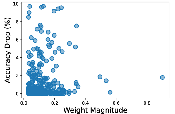
(a)

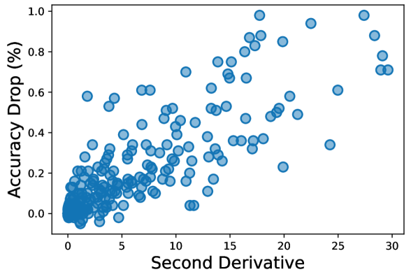
(b)

Figure 1. Impact of LeNet weight variation on MNIST: (a) Accuracy drop v.s. weight magnitude, where little correlation exists. (b) Accuracy drop v.s. second derivative of each weight, where strong correlation can be observed.

In this paper, contrary to the practice of all existing works that perform write-verify for every weight of a DNN, we establish and explore answers to the following problem.

Selective Write-Verify: Given a DNN architecture with weights $\mathbf{W_{0}}$ and a maximum acceptable accuracy drop $\delta A$, identify the smallest subset $\mathbf{W_{s}}\subseteq\mathbf{W_{0}}$ so that, when mapping the DNN to nvCiM platforms, by only writing-verifying weights in $\mathbf{W_{s}}$, the deployed network can have an accuracy no less than $\delta A$ below that of the original network.

One important feature for NVM devices is that the read process takes much shorter time than write (Shafiee and et al., 2016), especially for RRAMs and FeFETs. As such, reading the values of weights programmed into the devices and evaluating the corresponding accuracy of the DNN takes negligible amount of time compared with the write-verify process. We can leverage this feature to develop a heuristic approach to address the selective write-verify problem through iterative mapping, as shown in Alg. 1. For each weight in $\mathbf{W_{0}}$, we can first evaluate the impact of its variation on the accuracy of the DNN, which is referred to as its sensitivity in the remainder of this paper. Then we sort all the weights in descending order of sensitivity, and iteratively write-verify a group $p$ of the weights at a time (called programming granularity in Alg. 1) until the accuracy drop is below $\delta A$. In our experiments, we find that setting $p$ to be $5\%$ of the total number of weights is sufficient to provide the granularity for improving accuracy, while also avoiding too frequent evaluation of the accuracy of the mapped DNN. A critical question now is how to evaluate the sensitivity of a weight, which will be discussed in the next section.

Algorithm 1 SWIM ($\mathbf{W_{0}}$ , $\mathcal{Z}$, $A$, $\delta A$, $\mathbf{D}$, $p$)

1:  // INPUT: A trained DNN architecture $\mathcal{Z}$ with weights $\mathbf{W_{0}}$, original DNN accuracy $A$, the maximum accuracy drop allowed $\delta A$ after mapping to nvCiM, training dataset $\mathbf{D}$, and programming granularity $p$;

2:  Program all weights in $\mathbf{W_{0}}$ based on their locations in $\mathcal{Z}$ to the nvCiM platform;

3:  Calculate the sensitivity of all the weights;

4:  Sort $\mathbf{W_{0}}$ in the descending order of sensitivity.

5:  for ($i=0$; $i<(|\mathbf{W_{0}}|/p)$; $i++$) do

6:     Write-verify the weights $\mathbf{W_{0}}[i\times p+1:(i+1)\times p]$ based on their positions in $\mathcal{Z}$;

7:     Evaluate the accuracy $\tilde{A}$ of the mapped network on $\mathbf{D}$;

8:     if $A-\tilde{A}\leq\delta A$ then

9:        Break;

10:     end if

11:  end for

3.2. Sensitivity Analysis

Our goal is to find a way to evaluate the sensitivity for each weight. Intuitively, one would think that the magnitude of a weight would be a good indicator for sensitivity, and that, the larger the weight is, the more impact on the accuracy it would have when it is being perturbed. Unfortunately, our preliminary studies show that this is not the case. From experimental results in (Feinberg and et al., 2018), we assume a model where the amount of variances of NVM devices are independent of the value to be programmed. We perturb each weight in LeNet with the same additive Gaussian noise based on (Yao and et al., 2020) and evaluate the corresponding drop in the DNN accuracy for perturbing each weight, averaged over 100 Monte Carlo runs. From Fig.1, we can see that there is very weak correlation, if any, between the magnitude of weights and the accuracy drop that their variations cause. This observation is further confirmed in the experimental section, where we show that magnitude based selection approach would not yield good results. Below, we present a rigorous mathematical analysis, to establish a quite effective metric that can reflect the sensitivity of a weight.

As existing DNN optimization engines all map accuracy maximization to the minimization of a loss function, there is a strong correlation between the impact of a weight’s variation on accuracy and that on the loss function. As such, we resort to evaluating the sensitivity based on the latter.

For a DNN with a given labeled training dataset, loss $f$ is a function of a vector $\mathbf{w}$ formed by all the weights. Assume that the training is completed and the optimal weights identified are $\mathbf{\tilde{w}}$. With small variations of the weights around $\mathbf{\tilde{w}}$, i.e., $\mathbf{w}=\mathbf{\tilde{w}}+\mathbf{\Delta w}$, one can perform Taylor expansion on $f$ as follows:

(1) $$f(\mathbf{w})=f(\mathbf{\tilde{w}})+\frac{\partial f}{\partial\mathbf{\tilde{w}}}\Delta\mathbf{w}+\frac{1}{2}\Delta\mathbf{w}^{T}\mathcal{H}(\mathbf{\tilde{w}})\Delta\mathbf{w}+o(\Delta\mathbf{w}^{3})\vspace{-0.2cm}$$

where we use the compact notation $\frac{\partial f}{\partial\mathbf{\tilde{w}}}$ to represent $\frac{\partial f}{\partial\mathbf{w}}|_{\mathbf{w}=\mathbf{\tilde{w}}}$. Similar notation will be used throughout the paper. $\mathcal{H}(\mathbf{w})$ is the Hessian of $\mathbf{w}$ defined as

(2) $$\mathcal{H}(\mathbf{w})=\left[\begin{array}[]{ccc}\dfrac{\partial^{2}f}{\partial w_{1}^{2}}&\cdots&\dfrac{\partial^{2}f}{\partial w_{1}\partial w_{n}}\\ \vdots&\ddots&\vdots\\ \dfrac{\partial^{2}f}{\partial w_{n}\partial w_{1}}&\cdots&\dfrac{\partial^{2}f}{\partial w_{n}^{2}}\end{array}\right]$$

with $n$ being the total number of weights, i.e., length of $\mathbf{w}$.

As the neural network is trained to convergence through gradient descent, we have $\frac{\partial f}{\partial\mathbf{\tilde{w}}}=\mathbf{0}$. Accordingly, based on Eq. 1 the change in the loss function $\Delta f(\mathbf{w})$ brought by the weight variation $\Delta\mathbf{w}$ around $\mathbf{\tilde{w}}$ can be expressed as

(3) $$\Delta f(\mathbf{w})\approx\frac{1}{2}\Delta\mathbf{w}^{T}\mathcal{H}(\mathbf{\tilde{w}})\Delta\mathbf{w}\vspace{-0.1cm}$$

where we have ignored the higher-order terms.

Recall that $\Delta\mathbf{w}$ is device-specific and independent of the magnitude of $\mathbf{w}$ (Feinberg and et al., 2018). It is now clear that for a trained model, it is in fact the Hessian that plays a critical role in sensitivity. Unfortunately, the number of elements in Hessian is quadratically proportional to the number of weights. For example, a small neural network with one million weights ($10^{6}$) would require a Hessian with one trillion ($10^{12}$) elements, which is computationally impractical to evaluate.

To explore potential simplification, we notice that Eq. 3 can be expressed as

(4) $$\begin{split}\Delta f(\mathbf{w})&\approx\frac{1}{2}\sum^{n}_{i=1}\sum^{n}_{j=1}\mathcal{H}_{ij}\Delta w_{i}\Delta w_{j}\\ &=\frac{1}{2}\sum^{n}_{i=1}\mathcal{H}_{ii}(\Delta w_{i})^{2}+\frac{1}{2}\sum^{n}_{i\neq j}\mathcal{H}_{ij}\Delta w_{i}\Delta w_{j}\end{split}\vspace{-0.2cm}$$

where $\Delta w_{i}$ is the $i^{th}$ element of $\Delta\mathbf{w}$ and $\mathcal{H}_{ij}$ is the element in the $i^{th}$ row and $j^{th}$ column of $\mathcal{H(\mathbf{\tilde{w}})}$. To simplify Eq. 4, we assume that the change in the loss function caused by the variations in multiple weights is approximately the sum of those caused by each weight. As such, we only have to deal with one weight variation at a time. In this case, the cross terms can be discarded since either $\Delta w_{i}$ or $\Delta w_{j}$ is zero when $i\neq j$, and we have

(5) $$\Delta f(\mathbf{w})\approx\frac{1}{2}\sum^{n}_{i=1}\mathcal{H}_{ii}(\Delta w_{i})^{2}=\frac{1}{2}\sum^{n}_{i=1}\frac{\partial^{2}f}{\partial\tilde{w}_{i}^{2}}\Delta w_{i}^{2}\vspace{-0.2cm}$$

where $\tilde{w}_{i}$ is the $i^{th}$ element of $\mathbf{\tilde{w}}$. Extensive experimental study is conducted to confirm this approximation is acceptable.

Eq. 5 suggests that we only need to obtain the second derivative of each weight $\frac{\partial^{2}f}{\partial\tilde{w}_{i}^{2}}$ to evaluate the impact of weight variation on loss. By writing-verifying a weight $\tilde{w}_{i}$, we are essentially reducing $\Delta w_{i}$. Therefore, it is apparent that we shall assign higher priority to reduce the variation of those weights with higher second derivatives $\frac{\partial^{2}f}{\partial\tilde{w}_{i}^{2}}$. In other words, the second derivative can be used as a good sensitivity metric for SWIM. The effectiveness of this metric is confirmed in Fig. 1, where now with the same setting as in Fig. 1 strong correlation can be observed between the accuracy drop after a weight is perturbed and the second derivative of that weight (Pearson Correlation Coefficient being 0.83).

Finally, when two weights have the same second derivative, we use their magnitudes as the tie-breaker: the larger one will have a higher priority.

3.3. Second Derivative Calculation

One straightforward way to compute second derivative is to use finite difference method, i.e.,

(6) $$\frac{\partial^{2}f}{\partial\tilde{w}_{i}^{2}}\approx\frac{f(\tilde{w}_{i}+\Delta w)-2f(\tilde{w}_{i})+f(\tilde{w}_{i}-\Delta w)}{(\Delta w)^{2}}\vspace{-0.2cm}$$

where $\Delta w$ is a small positive number. However, in order to get $f(\tilde{w}_{i}+\Delta w)$ and $f(\tilde{w}_{i}-\Delta w)$, two passes of forward propagation are needed, after replacing $\tilde{w}_{i}$ with $\tilde{w}_{i}+\Delta w$ and $\tilde{w}_{i}-\Delta w$, respectively. For a network with one million weights, this requires two million passes of forward propagation.

Inspired by how the gradients of all the weights are efficiently computed through a single pass of forward and backpropagation based on the chain rule and the chain rule approximation of second derivatives presented in (LeCun and et al., 1990), below we present a method that can obtain second derivatives of all the weights in a similar way.

Let us start with the last fully connected (FC) layer of a DNN. The computation there can be expressed as

(7) $$\begin{split}\mathbf{P}=g_{a}(\mathbf{I}),\ \mathbf{O}=\mathbf{W}\cdot\mathbf{P}\end{split}\vspace{-0.3cm}$$

where $g_{a}$ is the activation function of the previous layer. $\mathbf{I}$ is the input vector to the activation function. $\mathbf{W}$ is the matrix containing the weights between the two layers. $\mathbf{P}$ is the output of the previous layer. $\mathbf{O}$ is the output of the last layer. We did not include the activation of the last layer as it can be merged into the loss function.

Consider a loss function $f(\mathbf{O})$ and we want to compute the second derivative for weights $\frac{\partial^{2}f}{\partial W_{ji}^{2}}$ and for inputs $\frac{\partial^{2}f}{\partial I_{i}^{2}}$. The former will be used as sensitivity and the latter will be used for further backpropagation to previous layers. Since $\mathbf{O}$ is a function of $\mathbf{W}$ and $\mathbf{P}$, we can apply the chain rule of the second derivative as

(8) $$\begin{split}\frac{\partial^{2}f}{\partial W_{ji}^{2}}=\frac{\partial^{2}f}{\partial O_{j}^{2}}\left(\frac{\partial O_{j}}{\partial W_{ji}}\right)^{2}+\frac{\partial f}{\partial O_{j}}\frac{\partial^{2}O_{j}}{\partial W_{ji}^{2}}=\frac{\partial^{2}f}{\partial O_{j}^{2}}\times P_{i}^{2}\end{split}\vspace{-0.3cm}$$

where the second equality comes from the fact that $O_{j}$ is a linear function of $W_{ji}$ so $\frac{\partial^{2}O_{j}}{\partial W_{ji}^{2}}=0$. Similarly, we can get the second derivative of the input

(9) $$\frac{\partial^{2}f}{\partial I_{i}^{2}}=g_{a}^{\prime}(P_{i})^{2}\sum_{j=1}^{|\mathbf{O}|}W_{ji}^{2}\frac{\partial^{2}f}{\partial O_{j}^{2}}-g_{a}^{\prime\prime}(P_{i})\frac{\partial f}{\partial I_{i}}\vspace{-0.1cm}$$

Assume we use ReLU as activation function. Then, $g_{a}^{\prime}(P_{i})=sign(P_{i})=sign(I_{i})$ and $g_{a}^{\prime\prime}=0$. Thus, second derivatives of the input can be expressed as:

(10) $$\frac{\partial^{2}f}{\partial I_{i}^{2}}=sign(I_{i})\sum_{j=1}^{\mathbf{|O|}}W_{ji}^{2}\frac{\partial^{2}f}{\partial O_{j}^{2}}\vspace{-0.1cm}$$

The backpropagation process of max pooling layers cancels derivatives of the deactivated inputs (i.e., the second derivatives of the deactivated inputs is zero). For ResNet and other models with skip connections, similar to backpropagation process used to calculate gradients, the second derivatives of different branches are summed up. Convolution layers, average pooling, and batch normalization layers can be cast in the same form as FC layers, so their backpropagation can share the same scheme as that for FC layers.

In summary, to get these second gradients, we simply need to compute the second derivative of the loss functions with respect to the output of the DNN, i.e., $\frac{\partial^{2}f}{\partial O_{j}^{2}}$. For L2 loss, $\frac{\partial^{2}f}{\partial O_{j}^{2}}=2$. For cross-entropy loss with softmax,

(11) $$\frac{\partial^{2}f}{\partial O_{j}^{2}}=\left(1-\frac{O_{j}}{\sum_{j}\exp(O_{j})}\right)\left(\frac{O_{j}}{\sum_{j}\exp(O_{j})}\right)\vspace{-0.1cm}$$

We can then follow Eq. 8 and Eq. 10 to backpropagate layer by layer.

Note that the first order gradient can be computed as

(12) $$\frac{\partial f}{\partial W_{ji}} =\frac{\partial f}{\partial O_{j}}\times P_{i}$$

(13) $$\frac{\partial f}{\partial I_{i}} =sign(I_{i})\sum_{j=1}^{\mathbf{|O|}}W_{ji}\frac{\partial f}{\partial O_{j}}\vspace{-0.2cm}$$

Comparing Eq. 12 and Eq. 13 with Eq. 8 and Eq. 10, we can find that the second derivative only requires an extra multiplication, and the time needed is negligible compared with convolution operations in forward propagation. If implemented efficiently, the second derivative calculation process of SWIM takes approximately the same amount of time and memory as conventional gradient computation. In addition, unlike gradient computation that needs to be repeated in each iteration of gradient descent, in SWIM only second derivative computation is done only once.

Table 1. Comparison of accuracy (%) and normalized write cycles (NWC) between SWIM and the baselines on LeNet for MNIST under different $\sigma$, the standard deviation specified in Eq. 16 before write-verify. Data are collected over 3,000 Monte Carlo runs and reported in mean$\pm$std format. Write cycles are normalized to those needed to write-verify all the weights. NWC $=0.0$ means no write-verify or in-situ training. NWC $=1.0$ for the three write-verify methods corresponds to the conventional method of writing-verifying all the weights.

$\sigma$	Method	Normalized Write Cycles (NWC)
		0.0	0.1	0.3	0.5	0.7	0.9	1.0
0.1	SWIM	$\uparrow$	98.49 $\pm$ 0.08	98.56 $\pm$ 0.08	98.57 $\pm$ 0.08	98.57 $\pm$ 0.08	98.57 $\pm$ 0.08	$\uparrow$
	Magnitude	97.96 $\pm$ 0.31	98.20 $\pm$ 0.19	98.41 $\pm$ 0.12	98.50 $\pm$ 0.09	98.54 $\pm$ 0.08	98.56 $\pm$ 0.08	98.58 $\pm$ 0.08
	Random		98.03 $\pm$ 0.26	98.17 $\pm$ 0.21	98.30 $\pm$ 0.16	98.42 $\pm$ 0.12	98.52 $\pm$ 0.09	$\downarrow$
	In-situ	$\downarrow$	98.39 $\pm$ 0.21	98.46 $\pm$ 0.19	98.47 $\pm$ 0.17	98.48 $\pm$ 0.16	98.50 $\pm$ 0.17	98.51 $\pm$ 0.17
0.15	SWIM	$\uparrow$	98.30 $\pm$ 0.13	98.52 $\pm$ 0.09	98.57 $\pm$ 0.08	98.57 $\pm$ 0.08	98.58 $\pm$ 0.08	$\uparrow$
	Magnitude	96.13 $\pm$ 1.23	97.33 $\pm$ 0.56	98.14 $\pm$ 0.21	98.43 $\pm$ 0.12	98.51 $\pm$ 0.10	98.56 $\pm$ 0.08	98.58 $\pm$ 0.08
	Random		96.53 $\pm$ 1.04	97.20 $\pm$ 0.65	97.73 $\pm$ 0.39	98.12 $\pm$ 0.23	98.45 $\pm$ 0.12	$\downarrow$
	In-situ	$\downarrow$	96.47 $\pm$ 1.00	96.59 $\pm$ 0.82	96.69 $\pm$ 0.84	96.72 $\pm$ 0.82	96.79 $\pm$ 0.85	96.84 $\pm$ 0.77
0.2	SWIM	$\uparrow$	98.12 $\pm$ 0.16	98.46 $\pm$ 0.09	98.55 $\pm$ 0.08	98.57 $\pm$ 0.08	98.58 $\pm$ 0.08	$\uparrow$
	Magnitude	94.46 $\pm$ 2.16	96.20 $\pm$ 1.11	97.65 $\pm$ 0.39	98.29 $\pm$ 0.14	98.45 $\pm$ 0.10	98.54 $\pm$ 0.08	98.58 $\pm$ 0.08
	Random		94.89 $\pm$ 1.90	96.13 $\pm$ 1.20	97.15 $\pm$ 1.43	97.88 $\pm$ 0.71	98.38 $\pm$ 0.20	$\downarrow$
	In-situ	$\downarrow$	95.33 $\pm$ 1.75	95.96 $\pm$ 1.36	96.42 $\pm$ 1.18	96.49 $\pm$ 1.09	96.69 $\pm$ 0.94	96.82 $\pm$ 0.80

4. Experimental Evalutaion

In this section, we first define the device variation model we use. Then, we describe a comprehensive study on the MNIST dataset to show the effectiveness of SWIM over the state-of-the-art under different device variations. After that, we use CIFAR-10 and Tiny ImageNet datasets to show its effectiveness in larger models.

4.1. Mapping and Impact of Device Variations

This paper is a proof concept to show the effectiveness of SWIM on temporal variations in the programming process, where the variation of each device is independent, so we use a simple yet realistic model to describe it.

For a weight represented by $M$ bits, let its desired value $\mathcal{W}_{des}$ be:

(14) $$\mathcal{W}_{des}=\sum_{i=0}^{M-1}{m_{i}\times 2^{i}}$$

where $m_{i}$ is the value of the $i^{th}$ bit of the desired weight value. We also assume the value programmed on each device is a Gaussian variable of $\mathcal{N}(g,\sigma^{2})$ where $g$ is the desired conductance value and $\sigma$ describes the level of uncertainty under device variation. Note that $\sigma$ is independent of $\mathcal{W}_{des}$ according to experimental observations (Feinberg and et al., 2018).

An $M$-bit weight can be mapped to $M/K$ $K$-bit devices, with the mapped value of the $i^{th}$ ($0\leq i\leq M/K-1$) device $g_{i}$ as:

(15) $$g_{i}=\mathcal{N}\left(\sum_{j=0}^{K-1}{m_{i\times K+j}\times 2^{j},\sigma^{2}}\right)\vspace{-0.2cm}$$

Note that negative weights are mapped in a similar manner.

Thus, when a weight is programmed, the actual value $\mathcal{W}_{map}$ mapped on the devices would be:

(16) $$\begin{split}\mathcal{W}_{map}&=\sum_{i=0}^{M/K-1}2^{i\times K}{\mathcal{N}\left(g_{i},\sigma^{2}\right)}\\ &=\mathcal{W}_{des}+\sum_{i=0}^{M/K-1}2^{i\times K}{\mathcal{N}(0,\sigma^{2})}\\ &=\mathcal{W}_{des}+\mathcal{N}\left(0,\sigma^{2}\sum_{i=0}^{M/K-1}{2^{i\times K\times 2}}\right)\end{split}\vspace{-0.5cm}$$

In the experiments below, we set $K=4$ as in (Jiang and et al., 2020) and follow the above model in simulating the write-verify process. Same as the standard practice discussed in Section 2.1, for each weight, we iteratively program the difference between the value on the device and the expected value until it is below 0.06. With the inherent randomness, it may take different weights different number of cycles to complete the write-verify: some may not need rewrite at all; while others need a lot. Statistically, the above model results in an average of 10 cycles over all the weights and a weight variation distribution with $\sigma=0.03$ after write-verify. These numbers are in line with those reported in (Shim and et al., 2020), which confirms the validity of our model and parameters.

4.2. Baselines and Metrics

In addition to the common practice of writing-verifying all weights the comparison with which is quite trivial, we choose three baselines for SWIM to compare with: 1) Random selection: each time we randomly select a group of weights from the ones that have not yet been selected to perform write-verify. 2) Magnitude based approach: we sort all the weights based on their magnitude and conduct write-verify with the largest ones first. 3) In-situ training: retrain the networks on-chip following the same method as that used in (Yao and et al., 2020). No write-verify is performed.

Because these methods have different programming mechanisms (write-verify vs. on-device training), we use the total number of write cycles as an indicator for the programming time, which is fair as writing NVM devices takes far more time than reading them and other operations. For the two write-verify baseline methods and SWIM, the model in Section 4.1 is applied in simulating and counting the number of write cycles. On the other hand, the number of writes in each iteration of in-situ training is equal to the number of weights that are selected for update in that iteration as no write-verify is done. To better compare different methods, we normalize the number of write cycles with respect to that used to write-verify all the weights in the DNN model under the same setting.

Note that for SWIM, random selection and magnitude based selection, $0.0\leq$ NWC $\leq 1.0$, but for in-situ training, NWC can exceed $1.0$ because the model can be trained for many iterations and need a large number of writes to update the weights. If we do not do any write-verify or in-situ training, then NWC $=0.0$. In our experiments, we vary the maximum allowed accuracy drop $\delta A$ for each method and collect the resulting NWC needed.

All models presented are quantized to the proper data precision and trained to converge on GPU before mapping to nvCiM. This training process is quantization-aware following (Jiang and et al., 2020) but does not take device variations into considerations. The experiments are conducted on GTX Titan-XP GPUs with the machine learning framework of PyTorch 1.8.1. Considering the randomness in device variations, all results shown in this paper are obtained over 3,000 Monte Carlo runs with verified convergence, and both mean and standard deviation are reported.

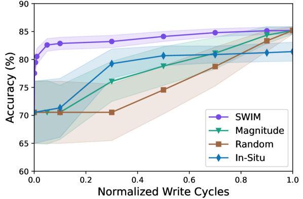
(a) ConvNet for CIFAR-10

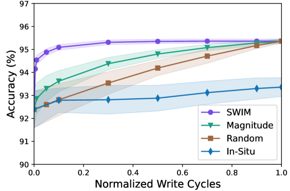
(b) ResNet-18 for CIFAR-10

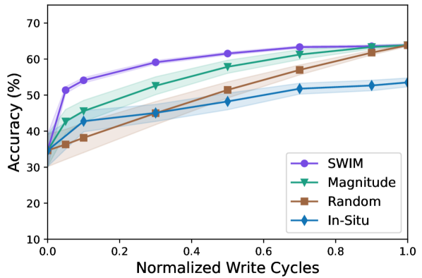
(c) ResNet-18 for Tiny ImageNet

Figure 2. Accuracy v.s. normalized write cycles (NWC) for SWIM and the baselines on three models: ConvNet and ResNet-18 for CIFAR-10 and ResNet-18 for Tiny ImageNet. Solid lines represent average accuracy and shadowed areas represent standard deviation, over 3,000 Monte Carlo runs using the device variation model.

4.3. Results for MNIST

We first show the effectiveness of SWIM on LeNet for the MNIST dataset. Both the weights and activation are quantized to 4 bits. The accuracy of this DNN model without the impact of device variation is 98.68%. The total number of weights of this model is $1.05\times 10^{5}$.

Although the typical standard deviation $\sigma$ for device variation model can be assumed to be $0.1$ before write-verify for most devices, certain emerging technologies may lead to higher variations especially before they become mature. To show the broad effectiveness of SWIM, we compare the performance of SWIM with the baseline methods over different $\sigma$ values. The results are shown in Table. 1. We can see that writing-verifying all the weights can mostly recover the model accuracy (i.e., 98.58% when NWC $=1.0$ for the three write-verify methods). While all the methods show a decrease in accuracy as NWC decreases, SWIM uses significantly fewer NWC than others to attain the same accuracy across all different $\sigma$ values. In addition, it also achieves a significantly lower standard deviation in accuracy than any other method over $3,000$ Monte Carlo runs, indicating that the accuracy would barely fluctuate across different devices.

Specifically, compared with the conventional practice of writing-verifying all the weights (NWC $=1.0$), with the typical variation ($\sigma=0.1$), SWIM only needs 50% of the write cycles (NWC $=0.5$, or $2\times$ speedup) to avoid any accuracy drop. Even with only 10% of the write cycles (NWC $=0.1$ or $10\times$ speedup), SWIM can attain an accuracy drop below $0.1\%$. On the other hand, the magnitude based approach, the random approach, and the in-situ training need an NWC close to 0.5, 0.9, and 0.9, respectively, for that accuracy. This translates to a speedup for SWIM of $5\times$, $9\times$, and $9\times$, respectively. SWIM remains effective even when $\sigma$ reaches $0.2$: compared with writing-verifying all the weights, by using 10% of the write cycles, it can achieve an accuracy drop of less than 0.5%. To achieve this accuracy, random approach and magnitude based approach need 70% and 50% of the write cycles respectively. And even with $10\times$ writes (NWC $=1.0$), in-situ training cannot achieve the same accuracy, indicating that it still needs more training iterations. While not shown in Table. 1, in-situ training can fully recover model accuracy (to 98.68%) using 32 NWC, which means it can achieve higher accuracy than the write-verify methods, but at the cost of a significantly larger number of writes and thus significantly longer programming time, as well as the additional hardware.

4.4. Results for CIFAR-10

We now show the effectiveness of SWIM on the CIFAR-10 dataset with two models ConvNet (Peng and et al., 2019) and ResNet-18 (He and et al., 2016). For these two models, both the weights and activation are quantized to 6 bits and $\sigma=0.1$ before write-verify. The accuracy without device variations for ConvNet is 86.07% and for ResNet-18 is 95.62%. With device variation and all the weights written-verified, the numbers are 85.19% and 95.36%. respectively. The total number of weights for ConvNet and ResNet-18 are $6.40\times 10^{6}$ and $1.12\times 10^{7}$, respectively.

Fig. 2 shows the comparison between SWIM and the baselines on ConvNets. Compared with writing-verifying all the weights, all the methods except SWIM see an accuracy drop over 10% when NWC is 0.1, while SWIM keeps the accuracy drop below 2.5%. From this figure, we can clearly see that SWIM has the smallest standard deviation in accuracy among all the methods, demonstrating its superior robustness. While not shown in Fig. 2, with NWC $=75$, in-situ training can fully recover model accuracy.

Fig. 2 shows the comparison between SWIM and the baselines on ResNet-18. Similar conclusions can be drawn here. Compared with writing-verifying all the weights, SWIM can preserve an accuracy drop of less than 0.5% using only 10% of the write cycles, while the other methods result in an accuracy drop of more than 2% for the same number of write cycles. In-situ training can fully recover model accuracy with 115 NWC.

4.5. Experiments on Tiny ImageNet

Finally, we show the effectiveness of SWIM on Tiny ImageNet with ResNet-18 (He and et al., 2016), following the same quantization setting and $\sigma$. The accuracy is 65.50% without device variation, and 64.84% with device variation and all weight written-verified. The total number of weights for this model is $1.13\times 10^{7}$.

Fig. 2 shows the comparison between SWIM and the baselines on ResNet-18 for Tiny ImageNet. As this is a more challenging task than CIFAR-10, we can see that the accuracy drops for all the methods are larger compared with those in Fig. 2. Even so, SWIM can achieve an accuracy less than 3% lower than that of writing-verifying all the weights using only 10% of the write cycles, fewest of all the methods. In-situ training can fully recover model accuracy in 155 NWC.

5. Conclusions

In this work, contrary to the common practice that write-verify all the weights of a DNN when mapping it to an nvCiM platform to combat device non-idealities, we show that it is only necessary to write-verify a small portion of them while maintaining the accuracy. As such, the programming time can be drastically reduced. We further introduce SWIM, which efficiently computes second derivatives that can be used to select weights for write-verify. Experimental results show up to 10x speedup compared with conventional write-verify schemes with little accuracy difference.

References

- (1)
- Chen and et al. (2016) Yu-Hsin Chen and et al. 2016. Eyeriss: A Spatial Architecture for Energy-Efficient Dataflow for Convolutional Neural Networks. In Proc. of ISCA. IEEE, 367–379.
- Feinberg and et al. (2018) Ben Feinberg and et al. 2018. Making memristive neural network accelerators reliable. In HPCA. IEEE, 52–65.
- He and et al. (2016) Kaiming He and et al. 2016. Deep residual learning for image recognition. In CVPR. 770–778.
- Jiang and et al. (2020) Weiwen Jiang and et al. 2020. Device-circuit-architecture co-exploration for computing-in-memory neural accelerators. IEEE Trans. Comput. 70, 4 (2020), 595–605.
- LeCun and et al. (1990) Yann LeCun and et al. 1990. Optimal Brain Damage. In Advances in Neural Information Processing Systems, Vol. 2. Morgan-Kaufmann.
- Peng and et al. (2019) Xiaochen Peng and et al. 2019. DNN+NeuroSim: An End-to-End Benchmarking Framework for Compute-in-Memory Accelerators with Versatile Device Technologies. In Proc. of IEDM.
- Shafiee and et al. (2016) Ali Shafiee and et al. 2016. ISAAC: A convolutional neural network accelerator with in-situ analog arithmetic in crossbars. In ACM SIGARCH Computer Architecture News, Vol. 44. 14–26. Publisher: ACM New York, NY, USA.
- Shim and et al. (2020) Wonbo Shim and et al. 2020. Two-step write–verify scheme and impact of the read noise in multilevel RRAM-based inference engine. Semiconductor Science and Technology 35, 11 (2020), 115026. Publisher: IOP Publishing.
- Sze and et al. (2017) Vivienne Sze and et al. 2017. Efficient processing of deep neural networks: A tutorial and survey. Proc. IEEE 105, 12 (2017), 2295–2329. Publisher: Ieee.
- Yan et al. (2022) Zheyu Yan, , and et al. 2022. RADARS: Memory Efficient Reinforcement Learning Aided Differentiable Neural Architecture Search. In ASP-DAC.
- Yan and et al. (2020) Zheyu Yan and et al. 2020. When single event upset meets deep neural networks: Observations, explorations, and remedies. In ASP-DAC.
- Yan and et al. (2021) Zheyu Yan and et al. 2021. Uncertainty Modeling of Emerging Device based Computing-in-Memory Neural Accelerators with Application to Neural Architecture Search. In ASP-DAC. IEEE, 859–864.
- Yao and et al. (2020) Peng Yao and et al. 2020. Fully hardware-implemented memristor convolutional neural network. Nature 577, 7792 (Jan. 2020), 641–646.