Vectorization of a thread-parallel
Jacobi singular value decomposition method

Abstract

The eigenvalue decomposition (EVD) of (a batch of) Hermitian matrices of order two has a role in many numerical algorithms, of which the one-sided Jacobi method for the singular value decomposition (SVD) is the prime example. In this paper the batched EVD is vectorized, with a vector-friendly data layout and the AVX-512 SIMD instructions of Intel CPUs, alongside other key components of a real and a complex OpenMP-parallel Jacobi-type SVD method, inspired by the sequential xGESVJ routines from LAPACK. These vectorized building blocks should be portable to other platforms that support similar vector operations. Unconditional numerical reproducibility is guaranteed for the batched EVD, sequential or threaded, and for the column transformations, that are, like the scaled dot-products, presently sequential but can be threaded if nested parallelism is desired. No avoidable overflow of the results can occur with the proposed EVD or the whole SVD. The measured accuracy of the proposed EVD often surpasses that of the xLAEV2 routines from LAPACK. While the batched EVD outperforms the matching sequence of xLAEV2 calls, speedup of the parallel SVD is modest but can be improved and is already beneficial with enough threads. Regardless of their number, the proposed SVD method gives identical results, but of somewhat lower accuracy than xGESVJ.

65F15, 65F25, 65Y05, 65Y10

1 Introduction

The eigenvalue decomposition (EVD) of a Hermitian or a symmetric matrix of order two [26] is a part of many numerical algorithms, some of which are implemented in the LAPACK [4] library, like the one-sided Jacobi-type algorithm [16, 17, 18] for the singular value decomposition (SVD) of general matrices. It also handles the $2\times 2$ terminal cases in the QR-based [19, 20] and the MRRR-based [13, 14] algorithms for the eigendecomposition of Hermitian/symmetric matrices. Its direct application, the two-sided Jacobi-type EVD method for symmetric [26] and Hermitian [22] matrices, has not been included in LAPACK but is widely known.

The first part of the paper aims to show that reliability of the $2\times 2$ symmetric/Hermitian EVD, produced by the LAPACK routines xLAEV2, can be improved by scaling the input matrix $A$ by an easily computable power of two. This preprocessing not only prevents the scaled eigenvalues from overflowing (and underflowing if possible), but also preserves the eigenvectors of a complex $A$ from becoming inaccurate and non-orthogonal in certain cases of subnormal components of $a_{12}=\bar{a}_{21}$. The proposed EVD formulas are branch-free, implying no if-else statements, but relying instead on the standard-conformant [23] handling of the special floating-point values by the $\min\!/\!\max$ functions. If the formulas are implemented in the SIMD fashion, they can compute several independent EVDs in one go, instead of one by one in a sequence.

An algorithm that performs the same operation on a collection (a “batch”) of inputs of the same or similar (usually small) dimensions is known as batched (see, e.g., [1, Sect. 10] and [2]). A vectorized, batched EVD of Hermitian matrices of order two is thus proposed, in a similar vein as the batched $2\times 2$ SVD from [35]. Recall that a SIMD vector instruction performs an operation on groups (called vectors) of scalars, packed into the lanes of vector registers, at roughly the cost of one (or few) scalar operation. For example, two vectors, each with $\mathtt{s}$ lanes, can be multiplied, each lane of the first vector by the corresponding lane of the second one, at a fraction of the time of $\mathtt{s}$ scalar multiplications. If a batch of input and output matrices is represented as a set of separate data streams, each containing the same-indexed elements of a particular sequence of matrices (e.g., all $a_{11}^{(\ell)}$), then a stream can be handled as one or more vectors, depending on the hardware’s vector width $\mathtt{s}$, such that, e.g., $a_{11}^{(\ell)}$ is held in the $(\ell\bmod\mathtt{s})$-th lane of the $\lfloor\ell/\mathtt{s}\rfloor$-th vector. Every major CPU architecture, like those from Intel, AMD, IBM, and ARM, offers vector operations with varying, but ever expanding vector widths and instruction subsets. Also, there are specialized vector engines, like NEC SX-Aurora TSUBASA with 2048-bit-wide registers. Thus, it is not a question should an algorithm be vectorized, but how to do that, if possible.

The second part of the paper focuses on vectorization of the one-sided Jacobi-type SVD for general matrices (but with at least as many rows as there are columns), in its basic form [16], as implemented in the xGESVJ LAPACK routines, without the rank-revealing QR factorization and other preprocessing [17, 18] of the more advanced xGEJSV routines. Both sets of routines are sequential by design, even though the used BLAS/LAPACK subroutines might be parallelized. The Jacobi-type method is not the fastest SVD algorithm available, but it provides the superior accuracy of the singular vectors and high relative accuracy of the singular values [12]. It is shown how the whole method (but with a parallel pivot strategy), i.e., all of its components, can be vectorized with the Intel AVX-512 instruction subset. Those BLAS-like components that are strategy-agnostic can be retrofitted to the xGESVJ routines.

Certain time-consuming components of the Jacobi-type SVD method, like the column pair updates, have for long been considered for vectorization [11]. In fact, any component realized with calls of optimized BLAS or LAPACK routines is automatically vectorized if the routines themselves are, such as dot-products and postmultiplications of a column pair by a rotation-like transformation. In the sequential method, however, only one transformation is generated per a method’s step, in essence by the EVD of a pivot Grammian matrix of order two, while a parallel method generates up to $\left\lfloor n/2\right\rfloor$ transformations per step, with $n$ being the number of columns of the iteration matrix. This sequence of independent EVDs is a natural candidate for vectorization that computes several EVDs at once, and for its further parallelization, applicable for larger $n$. Also, some vector platforms provide no direct support for complex arithmetic with vectors of complex values in the typical, interleaved $z=(\Re{z},\Im{z})$ representation, and thus the split one [41], with an accompanying set of BLAS-like operations, is convenient. In the split representation, as explained in Section 2.4.1, a complex array is kept as two real arrays, such that the $i$th complex element $z_{i}$ is represented by its real ($\Re{z_{i}}$) and imaginary ($\Im{z_{i}}$) parts, stored separately in the corresponding real arrays.

Batched matrix factorizations (like the tall-and-skinny QR) and decompositions (like a small-order Jacobi-type SVD) in the context of the blocked Jacobi-type SVD on GPUs have been developed in [34, 9], while the batched bidiagonalization on GPUs has been considered in [15]. Efficient batched kernels are ideal for acceleration of the blocked Jacobi-type SVD methods, but the non-blocked (pointwise) ones induce only batches of the smallest, $2\times 2$ EVD problems for the one-sided, and the SVD ones for the two-sided [29, 35] methods, what motivated developing of the proposed batched EVD.

The two mentioned parts of the paper further subdivide as follows. In Section 2 the vectorized batched EVD of Hermitian matrices of order two is developed and its numerical properties are assessed. In Section 3 the robust principles of (re-)scaling of the iteration matrix in the SVD method are laid out, such that the matrix can never overflow under inexact transformations, and a majority of the remaining components of the method is vectorized. In Section 4 the developed building blocks are put together to form a vectorized one-sided Jacobi-type SVD method (with a parallel strategy), that can be executed single- or multi-threaded, with identical outputs guaranteed in either case. Numerical testing is presented in Section 5. The paper concludes with a summary and some directions for further research in Section 6. Appendix contains most proofs and additional algorithms, code, and numerical results.

2 Vectorization of eigendecompositions of order two

Let $A$ be a symmetric (Hermitian) matrix of order two, $U$ an orthogonal (unitary) matrix of its eigenvectors, i.e., its diagonalizing Jacobi rotation, real [26] or complex [22], and $\Lambda$ a real diagonal matrix of its eigenvalues. In the complex case,

(1) $$A=U\Lambda U^{\ast},\quad U=\begin{bmatrix}\cos\varphi&-\mathrm{e}^{-\mathrm{i}\alpha}\sin\varphi\\ \mathrm{e}^{\mathrm{i}\alpha}\sin\varphi&\cos\varphi\end{bmatrix},\quad\Lambda=\begin{bmatrix}\lambda_{1}&0\\ 0&\lambda_{2}\end{bmatrix},$$

with $\varphi\in\left[-\pi/4,\pi/4\right]$ and $\alpha\in\left\langle-\pi,\pi\right]$, while $\alpha=0$ in the real case. The angles $\varphi$ and $\alpha$ are defined in terms of the elements of $A$, as detailed in Section 2.1. From Eq. 1 it follows by two matrix multiplications that

(2) $$A=\cos^{2}\varphi\begin{bmatrix}\lambda_{1}+\lambda_{2}\tan^{2}\varphi&\mathrm{e}^{-\mathrm{i}\alpha}\tan\varphi(\lambda_{1}-\lambda_{2})\\ \mathrm{e}^{\mathrm{i}\alpha}\tan\varphi(\lambda_{1}-\lambda_{2})&\lambda_{1}\tan^{2}\varphi+\lambda_{2}\end{bmatrix}.$$

Should $A$ be constructed from Eq. 2, e.g., for testing purposes, with its eigenvalues prescribed, then it suffices to ensure that $|\lambda_{1}|+|\lambda_{2}|\leq\nu/8$, where $\nu$ is the largest finite floating-point value, to get $\max|a_{ij}|\leq\nu/(4\sqrt{2})$. In Proposition 2.5 it is shown that such a bound on the magnitudes of the elements of $A$ guarantees that its eigenvalues will not overflow. If the bound does not hold, $A$ has to be downscaled to compute $\Lambda$.

One applicable power-of-two scaling algorithm was proposed in [35, subsection 2.1] in the context of the SVD of a general real or complex $2\times 2$ matrix, and is adapted for the EVD of a symmetric or Hermitian matrix $A$ of order two in Section 2.3.

Contrary to the standalone EVD, for orthogonalization of a pivot column pair in the Jacobi SVD algorithm it is sufficient to find the eigenvectors $U$ of their pivot Grammian matrix $A$, while its eigenvalues in $\Lambda$ are of no importance. If the orthogonalized pivot columns are also to be ordered in the iteration matrix non-increasingly with respect to their Frobenius norms, a permutation $P$ (as in, e.g., [34]) has to be found such that $\lambda_{1}^{\prime}\geq\lambda_{2}^{\prime}\geq 0$, where $\Lambda^{\prime}=P^{T}U^{\ast}AUP$, i.e., the pivot columns have to be transformed by multiplying them from the right by $UP$ instead of by $U$. For a comparison of the eigenvalues of $A$ to be made, it is only required that the eigenvalue with a smaller magnitude is finite, while the other one may be allowed to overflow.

2.1 Branch-free computation of the Jacobi rotations

Assume that $A$, represented by its lower triangle elements $a_{11}$, $a_{21}$, and $a_{22}$, has already been scaled. From the annihilation condition $U^{\ast}AU=\Lambda$, as shown in Section A.1 similarly to [22], but using the fused multiply-add operation with a single rounding of its result [23] (i.e., $\mathop{\mathrm{fma}}(a,b,c)=\mathop{\circ}(a\cdot b+c)$, where $\circ$ denotes the chosen rounding method), and assuming $\arg{0}=0$ for determinacy, it follows

(3) $$\lambda_{1}/\cos^{2}\varphi =(a_{22}\cdot\tan\varphi+2|a_{21}|)\cdot\tan\varphi+a_{11},$$

$$\lambda_{2}/\cos^{2}\varphi =(a_{11}\cdot\tan\varphi-2|a_{21}|)\cdot\tan\varphi+a_{22},$$

and for $\alpha$ from Eq. 1, in the complex case computed as in Eq. 12,

(4) $$\alpha=\arg{a_{21}},\quad\mathrm{e}^{\mathrm{i}\alpha}=a_{21}/|a_{21}|.$$

In the real case Eq. 4 leads to $\mathrm{e}^{\mathrm{i}\alpha}=\mathop{\mathrm{sign}}{a_{21}}=\pm 1$ (note, $\mathop{\mathrm{sign}}{\pm 0}=\pm 1$). Also,

(5) $$\tan\varphi=\frac{\tan(2\varphi)}{1+\sqrt{\tan(2\varphi)\cdot\tan(2\varphi)+1}},\qquad\cos\varphi=\frac{1}{\sqrt{\tan\varphi\cdot\tan\varphi+1}}.$$

With the methods from [35], and denoting by $\mathop{\mathrm{fl}}(x)=\mathop{\circ}(x)$ the rounded, floating-point representation of the value of the expression $x$, $\tan(2\varphi)$ is computed branch-free, as

(6) $$\tan(2\varphi)=\min\left(\mathop{\mathrm{fmax}}\left(\frac{2|a_{21}|}{|a|},0\right),\mathop{\mathrm{fl}}(\sqrt{\nu})\right)\cdot\mathop{\mathrm{sign}}{a},\qquad a=a_{11}-a_{22}.$$

The $\mathrm{fmax}$ call returns its second argument if the first one is $\mathtt{NaN}$ (when $|a_{21}|=|a|=0$).

The upper bound of $\mathop{\mathrm{fl}}(\sqrt{\nu})$ on $|\tan(2\varphi)|$ enables simplifying Eq. 5, since, when rounding to nearest, tie to even, $\mathop{\mathrm{fma}}(\mathop{\mathrm{fl}}(\sqrt{\nu}),\mathop{\mathrm{fl}}(\sqrt{\nu}),1)$ cannot overflow in single or double precision, so its square root in Eq. 5 can be computed faster than resorting to the $\mathop{\mathrm{hypot}}(x,y)=\sqrt{x^{2}+y^{2}}$ function. It can be verified (by a C program, e.g.) that the same bound ensures that Eq. 5 gives the correct answer for $\tan\varphi$ (i.e., $\pm 1$) instead of $\mathtt{NaN}$ when the unbounded $\tan(2\varphi)$ would be $\pm\infty$ due to $|a|=0$ and $|a_{21}|>0$.

By factoring out $\cos\varphi$ from $U$ in Eq. 1, $\sin\varphi=\tan\varphi\cdot\cos\varphi$ does not have to be computed, unless the eigenvectors are not required to be explicitly represented, since they can postmultiply a pivot column pair in the Jacobi SVD algorithm in this factored form, with $\cos\varphi$ and $\tan\varphi$, as in Eq. 21. In the Jacobi SVD algorithm, the ordering of the (always positive) eigenvalues of a pivot matrix is important for ordering the transformed pivot columns of the iteration matrix, i.e., for swapping them if $\lambda_{1}<\lambda_{2}$, while the actual eigenvalues have to be computed for the standalone, generic EVD only.

2.1.1 On $\mathtt{invsqrt}$

The $\mathop{\mathtt{invsqrt}}(\mathsf{x})=\mathop{\mathrm{fl}}(\mathsf{1}/\sqrt{\mathsf{x}})$ intrinsic function (a vectorized, presently not correctly rounded implementation of the standard’s recommended $\mathrm{rSqrt}$ function [23]) is appropriate for computation of the cosines directly from the squares of the secants ($\tan^{2}\varphi+1$) in Eq. 5, but it may not be available on another platform. A slower but unconditionally reproducible alternative, as explained in [38], is to compute

(7) $$\begin{gathered}\mathop{\mathrm{fl}}(\sec^{2}\varphi)=\mathop{\mathrm{fma}}(\mathop{\mathrm{fl}}(\tan\varphi),\mathop{\mathrm{fl}}(\tan\varphi),1),\quad\mathop{\mathrm{fl}}(\sec\varphi)=\mathop{\mathrm{fl}}(\sqrt{\mathop{\mathrm{fl}}(\sec^{2}\varphi)}),\\ \mathop{\mathrm{fl}}(\cos\varphi)=\mathop{\mathrm{fl}}(1/\mathop{\mathrm{fl}}(\sec\varphi)),\quad\mathop{\mathrm{fl}}(\sin\varphi)=\mathop{\mathrm{fl}}(\mathop{\mathrm{fl}}(\tan\varphi)/\mathop{\mathrm{fl}}(\sec\varphi)),\quad\end{gathered}$$

and optionally replace Eq. 3 by the potentially more accurately evaluated expressions

(8) $$\lambda_{1} =((a_{22}\cdot\tan\varphi+2|a_{21}|)\cdot\tan\varphi+a_{11})/\sec^{2}\varphi,$$

$$\lambda_{2} =((a_{11}\cdot\tan\varphi-2|a_{21}|)\cdot\tan\varphi+a_{22})/\sec^{2}\varphi.$$

Let $\delta_{1}$ be the relative rounding error accumulated in the process of computing $\mathop{\mathrm{fl}}(\cos\varphi)$ from $x=\mathop{\mathrm{fl}}(\sec^{2}\varphi)$. From Eq. 7, $\mathop{\mathrm{fl}}(\sec\varphi)=\sqrt{x}(1+\varepsilon_{0})=y$, and

(9) $$\mathop{\mathrm{fl}}(\cos\varphi)=\frac{1+\varepsilon_{1}}{y}=\frac{1+\varepsilon_{1}}{1+\varepsilon_{0}}\cdot\frac{1}{\sqrt{x}}=\delta_{1}\cdot\frac{1}{\sqrt{x}},\quad 0\leq\max\{|\varepsilon_{0}|,|\varepsilon_{1}|\}\leq\varepsilon,$$

where $\varepsilon=2^{-(p+1)}=0.5\mathop{\mathrm{ulp}}(1)$ is the machine precision when rounding to nearest, $p$ is the number of bits of significand ($23$, $52$, or $112$ for single, double, or quadruple precision), and $\mathop{\mathrm{ulp}}(x)=2^{\lfloor\lg|x|\rfloor-p}$. By minimizing and maximizing $\delta_{1}$ in Eq. 9 it follows

(10) $$\delta_{1}^{-}=\frac{1-\varepsilon}{1+\varepsilon}\leq\delta_{1}\leq\frac{1+\varepsilon}{1-\varepsilon}=\delta_{1}^{+}.$$

2.2 Implementation of complex arithmetic

Let $a$, $b$, $c$, and $d$ be complex values such that $d=a\cdot b+c$. By analogy with the real fused multiply-add operation, let such a ternary complex function and its value in floating-point be denoted as $\tilde{d}=\mathop{\mathrm{fl}}(d)=\mathop{\mathrm{fma}}(a,b,c)$. Then, $\tilde{d}$ can be computed with only two roundings for each of its components (as suggested in the cuComplex.h header in the CUDA toolkit), as

(11) $$\Re\tilde{d}=\mathop{\mathrm{fma}}(\Re{a},\Re{b},\mathop{\mathrm{fma}}(-\Im{a},\Im{b},\Re{c})),\quad\Im\tilde{d}=\mathop{\mathrm{fma}}(\Re{a},\Im{b},\mathop{\mathrm{fma}}(\Im{a},\Re{b},\Im{c})).$$

A branch-free way of computing the polar form of a complex value $z$ as $|z|\mathrm{e}^{\mathrm{i}\beta}$, with $\beta=\arg{z}$ and $\mathop{\mathrm{fl}}(|z|)=\mathop{\mathrm{hypot}}(\Re{z},\Im{z})\leq\nu$, was given in [35, Eq. (1)] as

(12) $$\mathop{\mathrm{fl}}(\cos\beta)=\mathop{\mathrm{fmin}}(|\Re{z}|/\mathop{\mathrm{fl}}(|z|),1)\cdot\mathop{\mathrm{sign}}{\Re{z}},\quad\mathop{\mathrm{fl}}(\sin\beta)=\Im{z}/\max\{\mathop{\mathrm{fl}}(|z|),\check{\mu}\},$$

where $\check{\mu}$ is the smallest subnormal positive non-zero real value. Floating-point operations must not trap on exceptions and subnormal numbers have to be supported as both inputs and outputs. The $\mathop{\mathrm{fmin}}$ and $\mathop{\mathrm{fmax}}$ functions have to return their second argument if the first one is $\mathtt{NaN}$, but the full C language [25] semantics is not required.

2.2.1 On $\mathtt{hypot}$

The $\mathtt{hypot}$ vector intrinsic function may not be available in another environment. It can be substituted [35] by a naïve yet fully vectorized and unconditionally reproducible Algorithm 1 (using the notation from Section 2.4), based on the well-known relations $\mathop{\mathrm{hypot}}(0,0)=0$ and (abusing the symbols $m$ and $M$)

(13) $$\begin{gathered}\sqrt{x^{2}+y^{2}}=M\sqrt{\left(\frac{x}{M}\right)^{2}+\left(\frac{y}{M}\right)^{2}}=M\sqrt{\left(\frac{m}{M}\right)^{2}+1}=M\sqrt{q^{2}+1},\\ q=m/M,\quad m=\min\{|x|,|y|\},\quad\nu\geq M=\max\{|x|,|y|\}>0.\end{gathered}$$

Algorithm 1 A naïve vectorized $\mathtt{hypot}$.

0:  vectors $\mathsf{x}$ and $\mathsf{y}$ with finite values in each lane

0:  $\mskip-5.0mu\approx\mskip-4.0mu\sqrt{\mathsf{x}^{\mathsf{2}}+\mathsf{y}^{\mathsf{2}}}$, not correctly rounded but without undue overflow in each lane

1:  $\mathsf{0}=\mathop{\mathtt{setzero}}();\quad\mathsf{1}=\mathop{\mathtt{set1}}(1.0);$ /​/ all vector lanes set to a constant

2:  $-\mathsf{0}=\mathop{\mathtt{set1}}(-0.0);\quad\mathsf{x}=\mathop{\mathtt{andnot}}(-\mathsf{0},\mathsf{x});\quad\mathsf{y}=\mathop{\mathtt{andnot}}(-\mathsf{0},\mathsf{y});$ /​/ $\mathsf{x}=|\mathsf{x}|$, $\mathsf{y}=|\mathsf{y}|$

3:  $\mathsf{m}=\mathop{\mathtt{min}}(\mathsf{x},\mathsf{y});\quad\mathsf{M}=\mathop{\mathtt{max}}(\mathsf{x},\mathsf{y});$

4:  $\mathsf{q}=\mathop{\mathtt{max}}(\mathop{\mathtt{div}}(\mathsf{m},\mathsf{M}),\mathsf{0});$ /​/ $\mathtt{max}$ replaces $0/0\to\mathtt{NaN}$ with $0$

5:  return  $\mathop{\mathtt{mul}}(\mathop{\mathtt{sqrt}}(\mathop{\mathtt{fmadd}}(\mathsf{q},\mathsf{q},\mathsf{1})),\mathsf{M});$

Lemma 2.1 gives the relative error bounds for $\mathop{\mathrm{hypot}}(x,y)$ if computed in the standard [23] floating-point arithmetic as in Algorithm 1, with (exactly representable) scalars $x$ and $y$ instead of vectors. In Eq. 13 and in the scalar Algorithm 1, $M>0$ implies $\mathop{\mathrm{fl}}(\mathop{\mathrm{hypot}}(x,y))>0$, while $M=0$ implies $q=0=\mathop{\mathrm{fl}}(\mathop{\mathrm{hypot}}(x,y))$ in the latter.

Lemma 2.1.

Let $\mathop{\mathrm{hypot}}(x,y)$ be defined by Eq. 13, and assume that neither overflow nor underflow occurs in the final multiplication of $M$ by $\mathop{\mathrm{fma}}(\mathop{\mathrm{fl}}(q),\mathop{\mathrm{fl}}(q),1)$. Then,

(14) $$\begin{gathered}\mathop{\mathrm{fl}}(\mathop{\mathrm{hypot}}(x,y))=\delta_{2}\mathop{\mathrm{hypot}}(x,y),\\ \delta_{2}^{-}=(1-\varepsilon)^{5/2}\sqrt{1-\varepsilon(2-\varepsilon)/2}<\delta_{2}<(1+\varepsilon)^{5/2}\sqrt{1+\varepsilon(2+\varepsilon)/2}=\delta_{2}^{+}.\end{gathered}$$

Proof 2.2.

See Section A.1.1.

Remark 2.3.

For all complex, representable values $z\neq 0$, $|\mathop{\mathrm{fl}}(z/\mathop{\mathrm{fl}}(|z|))|\leq\sqrt{2}$ in the standard rounding modes, since, from Eq. 13, $\mathop{\mathrm{fl}}(|z|)\geq\max\{|\Re{z}|,|\Im{z}|\}$, what, together with $z=|z|\mathrm{e}^{\mathrm{i}\beta}$ and Eq. 12, gives $1\geq|\mathop{\mathrm{fl}}(\cos\beta)|\geq|\mathop{\mathrm{fl}}(\sin\beta)|$ if $|\Re{z}|\geq|\Im{z}|$, or $1\geq|\mathop{\mathrm{fl}}(\sin\beta)|\geq|\mathop{\mathrm{fl}}(\cos\beta)|$ otherwise. In certain cases that do not satisfy the assumption of Lemma 2.1, $\mathop{\mathrm{fl}}(\mathrm{e}^{\mathrm{i}\alpha})$ from Eq. 4, computed by Eq. 13 or by another $\mathrm{hypot}$, might be quite inaccurate, with $|\mathop{\mathrm{fl}}(\mathrm{e}^{\mathrm{i}\alpha})|\leq\sqrt{2}$. Remark 2.4 shows that this bound is sharp.

Remark 2.4.

For all representable $x=\mathop{\mathrm{fl}}(x)$, $\mathop{\mathrm{fl}}(\mathop{\mathrm{hypot}}(x,x))=\mathop{\mathrm{fl}}(\mathop{\mathrm{fl}}(\sqrt{2})|x|)$ if computed as in Eq. 13. Let $\Psi_{\mathtt{T}}^{\circ}$ be a set of subnormal non-zero $x$, that depends on the implementation of $\mathrm{hypot}$, the datatype $\mathtt{T}$, and the rounding mode $\circ$ in effect, on which $\mathop{\mathrm{fl}}(\mathop{\mathrm{hypot}}(x,x))=|x|$. This set is non-empty with the default rounding (e.g., it contains $x=\check{\mu}$ for Algorithm 1 and for the tested math library’s $\mathrm{hypot}$), but it should be empty when rounding to $+\infty$. For $y=x\in\Psi_{\mathtt{T}}^{\circ}$, $\delta_{2}=1/\sqrt{2}$ in Eq. 14. If for a complex $z$ holds $|\Re{z}|=|\Im{z}|=|x|\in\Psi_{\mathtt{T}}^{\circ}$, then $\mathop{\mathrm{fl}}(|z|)=|x|$, and so $|\mathop{\mathrm{fl}}(\cos\beta)|=|\mathop{\mathrm{fl}}(\sin\beta)|=1$ in Eq. 12. This has serious consequences for accuracy of the eigenvectors computed by the complex LAPACK routines, as shown in Section 5.2. If $\mathop{\mathrm{fl}}(U)$ comes from Algorithm 2 or its single precision version, an inaccurate $\mathop{\mathrm{fl}}(\mathrm{e}^{\mathrm{i}\alpha})$ from Eq. 4, for which $|\mathop{\mathrm{fl}}(\mathrm{e}^{\mathrm{i}\alpha})|=\sqrt{2}$, is avoided in many cases if Eq. 18 implies a large enough upscaling.

2.3 Almost exact scaling of a Hermitian matrix of order two

A scaling of $A$ sufficient for finiteness of $\Lambda$ in floating-point is given in Proposition 2.5.

Proposition 2.5.

If for a Hermitian matrix $A$ of order two holds

(15) $$\hat{a}=\max_{1\leq j\leq i\leq 2}|a_{ij}|\leq\nu/(4\sqrt{2})=\tilde{\nu},$$

then no output from any computation in Eqs. 4, 5, 6, 7 and 8, including the resulting eigenvalues, can overflow, assuming the standard [23] non-stop floating-point arithmetic in at least single precision ($p\geq 23$) and rounding to the nearest, tie to even.

Moreover, barring any underflow of the results of those computations, the following relative error bounds hold for the quantities computed as in Eqs. 4, 5, 6 and 7:

(16) $$\begin{gathered}\begin{aligned} \mathop{\mathrm{fl}}(\cos\alpha)&=\delta_{\alpha}^{\prime}\cos\alpha\\ \mathop{\mathrm{fl}}(\sin\alpha)&=\delta_{\alpha}^{\prime\prime}\sin\alpha\end{aligned}\,,\quad 1-4.000000\,\varepsilon<\left\{\begin{gathered}\delta_{\alpha}^{\prime},\delta_{\alpha}^{\prime\prime}\\ |\mathop{\mathrm{fl}}(\mathrm{e}^{\pm\mathrm{i}\alpha})|\end{gathered}\right\}<1+4.000001\,\varepsilon,\\ \mathop{\mathrm{fl}}(\tan\varphi)=\delta_{\varphi}^{\mathbb{F}}\tan\varphi,\quad\begin{rcases}1-\hphantom{0}5.500000\,\varepsilon\\ 1-11.500000\,\varepsilon\end{rcases}<\delta_{\varphi}^{\mathbb{F}}<\begin{cases}1+\hphantom{0}5.500001\,\varepsilon,&\mathbb{F}=\mathbb{R},\\ 1+11.500004\,\varepsilon,&\mathbb{F}=\mathbb{C},\end{cases}\\ \mathop{\mathrm{fl}}(\cos\varphi)=\delta_{c}^{\mathbb{F}}\cos\varphi,\quad\begin{rcases}1-\hphantom{0}8.000000\,\varepsilon\\ 1-14.000000\,\varepsilon\end{rcases}<\delta_{c}^{\mathbb{F}}<\begin{cases}1+\hphantom{0}8.000002\,\varepsilon,&\mathbb{F}=\mathbb{R},\\ 1+14.000006\,\varepsilon,&\mathbb{F}=\mathbb{C},\end{cases}\end{gathered}$$

where $\mathbb{F}$ indicates whether $A$ is real or complex. For different ranges of $\delta_{1}$ or $\delta_{2}$ the bounds can be recalculated as described in Section A.3, as well as for a different rounding mode (while lowering the upper bound of $\mathop{\mathrm{fl}}(\sqrt{\nu})$ for $\mathop{\mathrm{fl}}(\tan 2\varphi)$ if required).

Proof 2.6.

The proof is presented in Section A.2.

Corollary 2.7 gives a practical scaling bound in the terms of the magnitudes of the components of the elements of $A$ and an exactly representable value based on $\nu$.

Corollary 2.7.

If a Hermitian matrix $A$ of order two is scaled such that

(17) $$\max_{1\leq j\leq i\leq 2}\max\{|\Re{a_{ij}}|,|\Im{a_{ij}}|\}\leq\tilde{\nu}/\sqrt{2}=\nu/8,$$

then the assumption Eq. 15 of Proposition 2.5 holds for $A$.

Proof 2.8.

From $\max\{|\Re{a_{ij}}|,|\Im{a_{ij}}|\}\leq\nu/8$ it follows $|a_{ij}|\leq\nu\sqrt{2}/8=\nu/(4\sqrt{2})=\tilde{\nu}$.

With $\eta=\left\lfloor\lg(\nu/8)\right\rfloor$, Eq. 17 implies the scaling factor $2^{\zeta}$ of a $A$ ($A^{\prime}=2^{\zeta}A$), where

(18) $$\begin{gathered}\zeta=\min\{\nu,\zeta_{11},\zeta_{22},\zeta_{21}^{\Re},\zeta_{21}^{\Im}\}\in\mathbb{Z},\\ \zeta_{ii}=\eta-\left\lfloor\lg|a_{ii}|\right\rfloor,\quad\zeta_{21}^{\Re}=\eta-\left\lfloor\lg|\Re{a_{21}}|\right\rfloor,\quad\zeta_{21}^{\Im}=\eta-\left\lfloor\lg|\Im{a_{21}}|\right\rfloor,\end{gathered}$$

while $\lg 0=-\infty$ and $\zeta$ is an integer exactly representable as a floating-point value.

The eigenvalues of $A^{\prime}$ in $\Lambda^{\prime}$ cannot overflow, but in $\Lambda\approx 2^{-\zeta}\Lambda^{\prime}$ might, where the approximate sign warns of a possibility that the values in $A$ small enough in magnitude become subnormal and lose their least significant bits when downscaling it with $\zeta<0$. Otherwise, the scaling of $A$ is exact, and some subnormal values might be raised into the normal range when $\zeta>0$. The scaled eigenvalues in $\Lambda^{\prime}$ could be kept alongside $\zeta$ in the cases where $\Lambda$ is expected to overflow or underflow, and compatibility with the LAPACK’s xLAEV2 routines is not required. Else, $\Lambda$ is returned by backscaling.

2.3.1 A serial eigendecomposition algorithm for Hermitian matrices of order two

Listing LABEL:l:1 shows a serial C implementation of the described eigendecomposition algorithm for a Hermitian matrix of order two. All untyped variables are in double precision. The computed values are equivalent to those from the vectorized Algorithm 2. The three branches in lines 9 and 10 are avoided in the vectorized code. Since the $\mathtt{frexp}$ function returns $0$ for the exponent of zero instead of a huge negative value, the lines 5 to 8 take care of this exception as in [38, subsection 2.1.1].

Listing 1: zsjac2: a serial eigendecomposition of a double precision Hermitian matrix $A$ of order two in C

⬇

1// input: $\!a_{11}$, $\!a_{22}$, $\!\Re{a_{21}}$, $\!\Im{a_{21}}$; output: $\!\cos\varphi$, $\!\cos\alpha\tan\varphi$, $\!\sin\alpha\tan\varphi$; $\!\lambda_{1}$, $\!\lambda_{2}$; $\!p$[,$\zeta^{\prime}$]

2int $\zeta_{11}$, $\zeta_{22}$, $\zeta_{21}^{\Re}$, $\zeta_{21}^{\Im}$, $\zeta_{\mathbb{R}}$, $\zeta_{\mathbb{C}}$, $\zeta$, $\zeta^{\prime}$, $\eta^{\prime}$ = DBL_MAX_EXP - 3; // $\eta^{\prime}=\eta+1=1021$

3double $\check{\mu}$ = DBL_TRUE_MIN, $\sqrt{\nu}$ = 1.34078079299425956E+154 /* sqrt(DBL_MAX) */;

4// determine $\zeta$ assuming all inputs are finite; avoid taking the exponent of $0$

5frexp(fmax(fabs($a_{11}$), $\check{\mu}$), &$\zeta_{11}$); $\zeta_{11}$ = $\eta^{\prime}$ - $\zeta_{11}$;

6frexp(fmax(fabs($a_{22}$), $\check{\mu}$), &$\zeta_{22}$); $\zeta_{22}$ = $\eta^{\prime}$ - $\zeta_{22}$;

7frexp(fmax(fabs($\Re{a_{21}}$), $\check{\mu}$), &$\zeta_{21}^{\Re}$); $\zeta_{21}^{\Re}$ = $\eta^{\prime}$ - $\zeta_{21}^{\Re}$;

8frexp(fmax(fabs($\Im{a_{21}}$), $\check{\mu}$), &$\zeta_{21}^{\Im}$); $\zeta_{21}^{\Im}$ = $\eta^{\prime}$ - $\zeta_{21}^{\Im}$;

9$\zeta_{\mathbb{R}}$ = (($\zeta_{11}$ <= $\zeta_{22}$) ? $\zeta_{11}$ : $\zeta_{22}$); $\zeta_{\mathbb{C}}$ = (($\zeta_{21}^{\Re}$ <= $\zeta_{21}^{\Im}$) ? $\zeta_{21}^{\Re}$ : $\zeta_{21}^{\Im}$);

10$\zeta$ = (($\zeta_{\mathbb{R}}$ <= $\zeta_{\mathbb{C}}$) ? $\zeta_{\mathbb{R}}$ : $\zeta_{\mathbb{C}}$); $\zeta^{\prime}$ = -$\zeta$; // Eq. 18

11// scale the input matrix $A$ by $2^{\zeta}$: $A^{\prime}=2^{\zeta}A$

12$\Re{a_{21}^{\prime}}$ = scalbn($\Re{a_{21}}$, $\zeta$); $\Im{a_{21}^{\prime}}$ = scalbn($\Im{a_{21}}$, $\zeta$);

13$a_{11}^{\prime}$ = scalbn($a_{11}$, $\zeta$); $a_{22}^{\prime}$ = scalbn($a_{22}$, $\zeta$);

14// find the polar form of $a_{21}^{\prime}=2^{\zeta}a_{21}$ as $|a_{21}^{\prime}|\mathrm{e}^{\mathrm{i}\alpha}$ using Eqs. 12, 13 and 4

15$|\Re{a_{21}^{\prime}}|$ = fabs($\Re{a_{21}^{\prime}}$); $|\Im{a_{21}^{\prime}}|$ = fabs($\Im{a_{21}^{\prime}}$);

16am = fmin($|\Re{a_{21}^{\prime}}|$, $|\Im{a_{21}^{\prime}}|$); aM = fmax($|\Re{a_{21}^{\prime}}|$, $|\Im{a_{21}^{\prime}}|$); mM = fmax(am / aM, 0.0);

17$|a_{21}^{\prime}|$ = sqrt(fma(mM, mM, 1.0)) * aM; // $\mathop{\mathrm{hypot}}(|\Re{a_{21}^{\prime}}|,|\Im{a_{21}^{\prime}}|)$ as in Eq. 13

18$\cos\alpha$ = copysign(fmin($|\Re{a_{21}^{\prime}}|$ / $|a_{21}^{\prime}|$, 1.0), $\Re{a_{21}^{\prime}}$);

19$\sin\alpha$ = $\Im{a_{21}^{\prime}}$ / fmax($|a_{21}^{\prime}|$, $\check{\mu}$);

20// compute the Jacobi rotation as in Section 2.1

21$o$ = $|a_{21}^{\prime}|$ * 2.0; $a$ = $a_{11}^{\prime}$ - $a_{22}^{\prime}$;

22$\tan{2\varphi}$ = copysign(fmin(fmax($o$ / fabs($a$), 0.0), $\sqrt{\nu}$), $a$); // Eq. 6

23$\tan\varphi$ = $\tan{2\varphi}$ / (1.0 + sqrt(fma($\tan{2\varphi}$, $\tan{2\varphi}$, 1.0))); // Eq. 5

24$\sec^{2}\varphi$ = fma($\tan\varphi$, $\tan\varphi$, 1.0); $\sec\varphi$ = sqrt($\sec^{2}\varphi$); $\cos\varphi$ = 1.0 / $\sec\varphi$; // Eq. 7

25$\cos\alpha\tan\varphi$ = $\cos\alpha$ * $\tan\varphi$; // optionally, $\cos\alpha\sin\varphi$ = $\cos\alpha\tan\varphi$ / $\sec\varphi$;

26$\sin\alpha\tan\varphi$ = $\sin\alpha$ * $\tan\varphi$; // optionally, $\sin\alpha\sin\varphi$ = $\sin\alpha\tan\varphi$ / $\sec\varphi$;

27// compute the (backscaled) eigenvalues as in Eq. 8

28$\lambda_{1}^{\prime}$ = fma($\tan\varphi$, fma($a_{22}^{\prime}$, $\tan\varphi$, $\hphantom{\text{-}}o$), $a_{11}^{\prime}$) / $\sec^{2}\varphi$;

29$\lambda_{2}^{\prime}$ = fma($\tan\varphi$, fma($a_{11}^{\prime}$, $\tan\varphi$, -$o$), $a_{22}^{\prime}$) / $\sec^{2}\varphi$;

30$\lambda_{1}$ = scalbn($\lambda_{1}^{\prime}$, $\zeta^{\prime}$); $\lambda_{2}$ = scalbn($\lambda_{2}^{\prime}$, $\zeta^{\prime}$); // optionally

31return (($\zeta^{\prime}$ << 1) | ($\lambda_{1}^{\prime}$ < $\lambda_{2}^{\prime}$)); // pack $\zeta^{\prime}$ and the permutation bit $p$

2.4 Intel AVX-512 vectorization

In the following, a $\mathtt{function}$ in the teletype font is as shorthand for the Intel AVX-512 C intrinsic $\mathtt{\_mm512\_function\_pd}$. A $\mathsf{variable}$ in the sans-serif font or a $\bm{bold}$ Greek letter without an explicitly specified type is assumed to be a vector of the type $\mathtt{\_\_m512d}$, with $\mathtt{s}=8$ double precision values (lanes). A variable named with a letter from the Fraktur font (e.g., $\mathfrak{m}$) represents an eight-bit lane mask of the type $\mathtt{\_\_mmask8}$ (see [24] for the datatypes and the vector instructions). Most, but not all, intrinsics correspond to a single instruction.

The chosen vectorization approach is Intel-specific for convenience, but it is meant to determine the minimal set of vector operations required (hardware-supported or emulated) on any platform that is considered to be targeted, either by that platform’s native programming facilities, or via some multi-platform interface in the spirit of the SLEEF [39] vectorized C math library, e.g., or, if possible, by the compiler’s auto-vectorizer, as it has partially been done with the Intel Fortran compiler for the batched generalized eigendecomposition of pairs of Hermitian matrices of order two, one of them being positive definite, by the Hari–Zimmermann method [40, subsection 6.2].

2.4.1 Data storage and the split complex representation

For simplicity and performance, a real vector $\mathbf{x}$ of length $m$ is assumed to be contiguous in memory, aligned to a multiple of the larger of the vector size and the cache-line size (on Intel CPUs they are both $64\,\mathrm{B}$), and zero-padded at its end to the optimal length $\tilde{m}$, where

(19) $$\tilde{m}=\begin{cases}m,&\text{if }m\bmod\mathtt{s}=0,\\ m+(\mathtt{s}-(m\bmod\mathtt{s})),&\text{otherwise}.\end{cases}$$

If $\mathbf{z}$ is a complex array, it is kept as two real non-overlapping ones, $\Re{\tilde{\mathbf{z}}}$ and $\Im{\tilde{\mathbf{z}}}$ (for the real and the imaginary parts, respectively), laid out in this split form as

(20) $$\Re{\tilde{\mathbf{z}}}=\begin{bmatrix}\Re{\mathbf{z}}\\ \mathbf{0}_{\tilde{m}-m}\end{bmatrix},\qquad\Im{\tilde{\mathbf{z}}}=\begin{bmatrix}\Im{\mathbf{z}}\\ \mathbf{0}_{\tilde{m}-m}\end{bmatrix},$$

where the blocks $\mathbf{0}_{\tilde{m}-m}$ of zeros are the minimal padding that makes the length of the real as well as of the imaginary block a multiple of the number of SIMD lanes ($\mathtt{s}$), with $\tilde{m}$ from Eq. 19. A complex $m\times n$ matrix $G$ is kept as two real $\tilde{m}\times n$ matrices,

$$\Re{G}=\begin{bmatrix}\Re{g_{1}}&\Re{g_{2}}&\cdots&\Re{g_{n}}\\ \mathbf{0}_{\tilde{m}-m}&\mathbf{0}_{\tilde{m}-m}&\cdots&\mathbf{0}_{\tilde{m}-m}\end{bmatrix},\quad\Im{G}=\begin{bmatrix}\Im{g_{1}}&\Im{g_{2}}&\cdots&\Im{g_{n}}\\ \mathbf{0}_{\tilde{m}-m}&\mathbf{0}_{\tilde{m}-m}&\cdots&\mathbf{0}_{\tilde{m}-m}\end{bmatrix},$$

i.e., each column $g_{j}$ of $G$, where $1\leq j\leq n$, is split into the real ($\Re{g_{j}}$) and the imaginary ($\Im{g_{j}}$) part, as in Eq. 20. The leading dimensions of $\Re{G}$ and $\Im{G}$ may differ, but each has to be a multiple of $\mathtt{s}$ to keep all padded real columns properly aligned.

The split form has been used for efficient complex matrix multiplication kernels [41] and for the generalized SVD computation by the implicit Hari–Zimmermann algorithm on GPUs [37]. Intel CPUs have no native complex-specific arithmetic instructions operating on vectors of at least single precision complex numbers in the customary, interleaved representation, so a manual implementation of the vectorized complex arithmetic is inevitable, for what the split representation is more convenient.

A conversion of the customary representation of complex arrays to and back from the split form, in both vectorized and parallel fashion, is described in Appendix E.

An input batch $(A^{(\ell)})_{\ell=1}^{r}$ of Hermitian matrices of order two is kept as a collection of one-dimensional real arrays $\tilde{\mathbf{a}}_{11}$, $\tilde{\mathbf{a}}_{22}$, $\Re{\tilde{\mathbf{a}}_{21}}$, $\Im{\tilde{\mathbf{a}}_{21}}$, of length $\tilde{r}$ and with layout Eq. 20, where $\tilde{r}$ is calculated from $r$ as in Eq. 19, $(\tilde{\mathbf{a}}_{11})_{\ell}=a_{11}^{(\ell)}$, $(\tilde{\mathbf{a}}_{22})_{\ell}=a_{22}^{(\ell)}$, $(\Re{\tilde{\mathbf{a}}_{21}})_{\ell}=\Re{a_{21}^{(\ell)}}$, $(\Im{\tilde{\mathbf{a}}_{21}})_{\ell}=\Im{a_{21}^{(\ell)}}$. The output unpermuted eigenvalue matrices $(\Lambda^{(\ell)})_{\ell=1}^{r}$ are stored as the arrays $\tilde{\bm{\lambda}}_{1}=(\lambda_{1}^{(\ell)})_{\ell=1}^{\tilde{r}}$ and $\tilde{\bm{\lambda}}_{2}=(\lambda_{2}^{(\ell)})_{\ell=1}^{\tilde{r}}$. The corresponding Jacobi rotations’ parameters are kept in the arrays $\cos\tilde{\bm{\varphi}}$, $\cos\tilde{\bm{\alpha}}\tan\tilde{\bm{\varphi}}$, and $\sin\tilde{\bm{\alpha}}\tan\tilde{\bm{\varphi}}$. If $\lambda_{1}^{(\ell)}<\lambda_{2}^{(\ell)}$ then the permutation $P^{(\ell)}=\left[\begin{smallmatrix}0&1\\ 1&0\end{smallmatrix}\right]$, else $P^{(\ell)}=\left[\begin{smallmatrix}1&0\\ 0&1\end{smallmatrix}\right]$, what is compactly encoded by setting the $((\ell-1)\bmod\mathtt{s})$-th bit of a bitmask $\mathfrak{p}$ to $1$ or $0$, respectively.

2.4.2 Vectorized eigendecomposition of a batch of Hermitian matrices of order two

Based on Sections 2.1, 2.2 and 2.3, Algorithm 2 implements a vectorized, branch-free, unconditionally reproducible eigendecomposition method for at most $\mathtt{s}$ Hermitian matrices of order two in double precision. Although presented with the AVX512DQ instruction subset, only the basic, AVX512F subset is required. The order of the statements slightly differs from the one in the actual code, for legibility. For easier understanding of the vectorization, the lines of Algorithm 2 are suffixed by the corresponding line numbers of the serial algorithm from Listing LABEL:l:1 in brackets.

Algorithm 3 builds on Algorithm 2 and computes the eigendecomposition of a batch of Hermitian matrices of order two in parallel, where each OpenMP thread executes Algorithm 2 in sequence over a (not necessarily contiguous) subset of the input’s vectors. No dependencies exist between the iterations of the parallel-for loop of Algorithm 3, so it can be generalized by distributing its input over several machines.

Algorithms 9 and 10, detailed in Appendix B, are the specializations of Algorithms 2 and 3, respectively, for real symmetric matrices. There, $\mathrm{e}^{\mathrm{i}\tilde{\bm{\alpha}}}\tan\tilde{\bm{\varphi}}=\cos\tilde{\bm{\alpha}}\tan\tilde{\bm{\varphi}}=\mathop{\mathrm{sign}}\tilde{\mathbf{a}}_{21}\cdot\tan\tilde{\bm{\varphi}}$ elementwise.

Converting Algorithms 2 and 3 and Algorithms 9 and 10 to single precision, with $\mathtt{s}=16$, requires redefining $\nu=\mathtt{FLT\_MAX}$, $\mathop{\mathrm{fl}}(\sqrt{\nu})=\text{{1.844674297E+19}}$, $\check{\mu}=\mathtt{FLT\_TRUE\_MIN}$, $\eta=\mathtt{FLT\_MAX\_EXP}-4$ and switching to $\mathtt{\_mm512\_\cdots\_ps}$ intrinsics, $\mathtt{\_\_m512}$ vectors, and $\mathtt{\_\_mmask16}$ bitmasks, while the relative error bounds in Proposition 2.5 still hold. The serial code from Listing LABEL:l:1 can be similarly converted.

The algorithms can be implemented in a scalar fashion ($\mathtt{s}=1$), as in Listing LABEL:l:1, thus enabling access to the higher-precision, scalar-only datatypes, such as extended precision, or in a pseudo-scalar way of, e.g., GPU programming models, where each thread executes the scalar code over a different data in the same layout as proposed here. An implementation in CUDA is discussed in Appendix J.

Algorithm 2 $\mathtt{z8jac2}$: a vectorized eigendecomposition of at most $\mathtt{s}$ double precision Hermitian matrices of order two with the Intel’s AVX-512 intrinsics.

0:  $\mathtt{i}$; addresses of $\tilde{\mathbf{a}}_{11},\tilde{\mathbf{a}}_{22},\Re{\tilde{\mathbf{a}}_{21}},\Im{\tilde{\mathbf{a}}_{21}},\cos\tilde{\bm{\varphi}},\cos\tilde{\bm{\alpha}}\tan\tilde{\bm{\varphi}},\sin\tilde{\bm{\alpha}}\tan\tilde{\bm{\varphi}},\tilde{\bm{\lambda}}_{1},\tilde{\bm{\lambda}}_{2},\mathtt{p}$

0:  $\mathop{\mathsf{cos}}\varphi,\mathop{\mathsf{cos}}\alpha\mathop{\mathsf{tan}}\varphi,\mathop{\mathsf{sin}}\alpha\mathop{\mathsf{tan}}\varphi;\bm{\lambda}_{1},\bm{\lambda}_{2};\mathfrak{p}$ /​/ a permutation-indicating bitmask/​/ vectors with all lanes set to a compile-time constant

1:  $-\mathsf{0}=\mathop{\mathtt{set1}}(-0.0);\quad\mathsf{0}=\mathop{\mathtt{setzero}}();\quad\mathsf{1}=\mathop{\mathtt{set1}}(1.0);\quad\bm{\nu}=\mathop{\mathtt{set1}}(\mathtt{DBL\_MAX});$

2:  $\sqrt{\bm{\nu}}=\mathop{\mathtt{set1}}(\text{{1.34078079299425956E+154}});$ /​/ $\mathop{\mathrm{fl}}(\sqrt{\nu})$ from Eq. 6

3:  $\check{\bm{\mu}}=\mathop{\mathtt{set1}}(\mathtt{DBL\_TRUE\_MIN});\quad\bm{\eta}=\mathop{\mathtt{set1}}(1020.0);$ /​/ $\eta=(\mathtt{DBL\_MAX\_EXP}-1)-3$/​/ aligned loads of the $\mathtt{i}$th input vectors, e.g., $\mathsf{a}_{11}=\mathop{\mathtt{load}}(\tilde{\mathbf{a}}_{11}+\mathtt{i})$, happen here/​/ determine the scaling exponents $\bm{\zeta}$ from Eq. 18 and scale $\mathsf{A}\to\mathsf{2}^{\bm{\zeta}}\mathsf{A}$

4:  $\bm{\zeta}_{11}=\mathop{\mathtt{sub}}(\bm{\eta},\mathop{\mathtt{getexp}}(\mathsf{a}_{11}));\quad\bm{\zeta}_{22}=\mathop{\mathtt{sub}}(\bm{\eta},\mathop{\mathtt{getexp}}(\mathsf{a}_{22}));$ /​/ $[\ref{ll:5},\ref{ll:6}]$

5:  $\bm{\zeta}_{21}^{\Re}=\mathop{\mathtt{sub}}(\bm{\eta},\mathop{\mathtt{getexp}}(\Re{\mathsf{a}_{21}}));\quad\bm{\zeta}_{21}^{\Im}=\mathop{\mathtt{sub}}(\bm{\eta},\mathop{\mathtt{getexp}}(\Im{\mathsf{a}_{21}}));$ /​/ $[\ref{ll:7},\ref{ll:8}]$

6:  $\bm{\zeta}=\mathop{\mathtt{min}}(\bm{\nu},\mathop{\mathtt{min}}(\mathop{\mathtt{min}}(\bm{\zeta}_{11},\bm{\zeta}_{22}),\mathop{\mathtt{min}}(\bm{\zeta}_{21}^{\Re},\bm{\zeta}_{21}^{\Im})));$ /​/ $[\ref{ll:9},\ref{ll:10}]$

7:  $-\bm{\zeta}=\mathop{\mathtt{xor}}(\bm{\zeta},-\mathsf{0});$ /​/ $\mathop{\mathtt{xor}}(\mathsf{x},-\mathsf{0})$ flips the sign bits in $\mathsf{x}$; optionally, store $-\bm{\zeta}\quad[\ref{ll:10}]$

8:  $\Re{\mathsf{a}_{21}}=\mathop{\mathtt{scalef}}(\Re{\mathsf{a}_{21}},\bm{\zeta});\quad\Im{\mathsf{a}_{21}}=\mathop{\mathtt{scalef}}(\Im{\mathsf{a}_{21}},\bm{\zeta});$ /​/ $\mathsf{a}_{21}=\mathsf{2}^{\bm{\zeta}}\mathsf{a}_{21}\quad[\ref{ll:12}]$

9:  $\mathsf{a}_{11}=\mathop{\mathtt{scalef}}(\mathsf{a}_{11},\bm{\zeta});\quad\mathsf{a}_{22}=\mathop{\mathtt{scalef}}(\mathsf{a}_{22},\bm{\zeta});$ /​/ $\mathsf{a}_{ii}=\mathsf{2}^{\bm{\zeta}}\mathsf{a}_{ii}\quad[\ref{ll:13}]$/​/ find the polar form of $\mathsf{a}_{21}$ using Eqs. 4 and 12

10:  $|\Re{\mathsf{a}_{21}}|=\mathop{\mathtt{andnot}}(-\mathsf{0},\Re{\mathsf{a}_{21}});$ /​/ $\mathop{\mathtt{andnot}}(-\mathsf{0},\mathsf{x})=\mathsf{x}\wedge\neg{-\mathsf{0}}\quad[\ref{ll:15}]$

11:  $|\Im{\mathsf{a}_{21}}|=\mathop{\mathtt{andnot}}(-\mathsf{0},\Im{\mathsf{a}_{21}});$ /​/ $\mathtt{abs}$ could also be used to clear the sign bits$\quad[\ref{ll:15}]$

12:  $\mathop{\mathsf{sgn}}(\Re{\mathsf{a}_{21}})=\mathop{\mathtt{and}}(\Re{\mathsf{a}_{21}},-\mathsf{0});$ /​/ $\mathop{\mathtt{and}}(\mathsf{x},-\mathsf{0})$ extracts the sign bits$\quad[\ref{ll:18}]$

13:  $|\mathsf{a}_{21}|=\mathop{\mathtt{hypot}}(|\Re{\mathsf{a}_{21}}|,|\Im{\mathsf{a}_{21}}|);$ /​/ inline Algorithm 1$\quad[\ref{ll:16},\ref{ll:17}]$

14:  $|\mathop{\mathsf{cos}}\alpha|=\mathop{\mathtt{min}}(\mathop{\mathtt{div}}(|\Re{\mathsf{a}_{21}}|,|\mathsf{a}_{21}|),\mathsf{1});$ /​/ $\mathtt{min}$ replaces $0/0\to\mathtt{NaN}$ with $1\quad[\ref{ll:18}]$

15:  $\mathop{\mathsf{cos}}\alpha=\mathop{\mathtt{or}}(|\mathop{\mathsf{cos}}\alpha|,\mathop{\mathsf{sgn}}(\Re{\mathsf{a}_{21}}));$ /​/ $\mathtt{or}$ transfers the sign bits to positive values$\ [\ref{ll:18}]$

16:  $\mathop{\mathsf{sin}}\alpha=\mathop{\mathtt{div}}(\Im{\mathsf{a}_{21}},\mathop{\mathtt{max}}(|\mathsf{a}_{21}|,\check{\bm{\mu}}));$ /​/ $\mathtt{max}$ replaces $0$ with $\check{\mu}\quad[\ref{ll:19}]$/​/ compute $\mathop{\mathsf{cos}}\varphi$ and $\mathsf{e}^{\mathsf{i}\alpha}\mathop{\mathsf{tan}}\varphi$ (or $\mathsf{e}^{\mathsf{i}\alpha}\mathop{\mathsf{sin}}\varphi$)

17:  $\mathsf{o}=\mathop{\mathtt{scalef}}(|\mathsf{a}_{21}|,\mathsf{1});\quad\mathsf{a}=\mathop{\mathtt{sub}}(\mathsf{a}_{11},\mathsf{a}_{22});$ /​/ Eq. 6$\quad[\ref{ll:21}]$

18:  $|\mathsf{a}|=\mathop{\mathtt{andnot}}(-\mathsf{0},\mathsf{a});\quad\mathop{\mathsf{sgn}}(\mathsf{a})=\mathop{\mathtt{and}}(\mathsf{a},-\mathsf{0});$ /​/ Eq. 6$\quad[\ref{ll:22}]$

19:  $\mathop{\mathsf{tan}}2\varphi=\mathop{\mathtt{or}}(\mathop{\mathtt{min}}(\mathop{\mathtt{max}}(\mathop{\mathtt{div}}(\mathsf{o},|\mathsf{a}|),\mathsf{0}),\sqrt{\bm{\nu}}),\mathop{\mathsf{sgn}}(\mathsf{a}));$ /​/ Eq. 6$\quad[\ref{ll:22}]$

20:  $\mathop{\mathsf{sec}^{\mathsf{2}}}2\varphi=\mathop{\mathtt{fmadd}}(\mathop{\mathsf{tan}}2\varphi,\mathop{\mathsf{tan}}2\varphi,\mathsf{1});$ /​/ $\sec^{2}{2\varphi}<\infty\quad[\ref{ll:23}]$

21:  $\mathop{\mathsf{tan}}\varphi=\mathop{\mathtt{div}}(\mathop{\mathsf{tan}}2\varphi,\mathop{\mathtt{add}}(\mathsf{1},\mathop{\mathtt{sqrt}}(\mathop{\mathsf{sec}^{\mathsf{2}}}2\varphi)));$ /​/ Eq. 5$\quad[\ref{ll:23}]$

22:  $\mathop{\mathsf{sec}^{\mathsf{2}}}\varphi=\mathop{\mathtt{fmadd}}(\mathop{\mathsf{tan}}\varphi,\mathop{\mathsf{tan}}\varphi,1);$ /​/ Eq. 7$\quad[\ref{ll:24}]$

23:  $\mathop{\mathsf{sec}}\varphi=\mathop{\mathtt{sqrt}}(\mathop{\mathsf{sec}^{\mathsf{2}}}\varphi);\quad\mathop{\mathsf{cos}}\varphi=\mathop{\mathtt{div}}(\mathsf{1},\mathop{\mathsf{sec}}\varphi);$ /​/ Eq. 7$\quad[\ref{ll:24}]$

24:  $\mathop{\mathsf{cos}}\alpha\mathop{\mathsf{tan}}\varphi=\mathop{\mathtt{mul}}(\mathop{\mathsf{cos}}\alpha,\mathop{\mathtt{tan}}\varphi);$ /​/ $\mathop{\mathsf{cos}}\alpha\mathop{\mathsf{sin}}\varphi=\mathop{\mathtt{div}}(\mathop{\mathsf{cos}}\alpha\mathop{\mathsf{tan}}\varphi,\mathop{\mathsf{sec}}\varphi);\quad[\ref{ll:25}]$

25:  $\mathop{\mathsf{sin}}\alpha\mathop{\mathsf{tan}}\varphi=\mathop{\mathtt{mul}}(\mathop{\mathsf{sin}}\alpha,\mathop{\mathtt{tan}}\varphi);$ /​/ $\mathop{\mathsf{sin}}\alpha\mathop{\mathsf{sin}}\varphi=\mathop{\mathtt{div}}(\mathop{\mathsf{sin}}\alpha\mathop{\mathsf{tan}}\varphi,\mathop{\mathsf{sec}}\varphi);\quad[\ref{ll:26}]$/​/ compute the eigenvalues (aligned stores of the results also happen here)

26:  $\bm{\lambda}_{1}^{\prime}=\mathop{\mathtt{div}}(\mathop{\mathtt{fmadd}}(\mathop{\mathsf{tan}}\varphi,\mathop{\mathtt{fmadd}}(\mathsf{a}_{22},\mathop{\mathsf{tan}}\varphi,\mathsf{o}),\mathsf{a}_{11}),\mathop{\mathsf{sec}^{\mathsf{2}}}\varphi);$ /​/ Eq. 8$\quad[\ref{ll:28}]$

27:  $\bm{\lambda}_{2}^{\prime}=\mathop{\mathtt{div}}(\mathop{\mathtt{fmadd}}(\mathop{\mathsf{tan}}\varphi,\mathop{\mathtt{fmsub}}(\mathsf{a}_{11},\mathop{\mathsf{tan}}\varphi,\mathsf{o}),\mathsf{a}_{22}),\mathop{\mathsf{sec}^{\mathsf{2}}}\varphi);$ /​/ Eq. 8$\quad[\ref{ll:29}]$

28:  $\bm{\lambda}_{1}=\mathop{\mathtt{scalef}}(\bm{\lambda}_{1}^{\prime},-\bm{\zeta});\quad\bm{\lambda}_{2}=\mathop{\mathtt{scalef}}(\bm{\lambda}_{2}^{\prime},-\bm{\zeta});$ /​/ backscale $\bm{\lambda}_{1}$ and $\bm{\lambda}_{2}\quad[\ref{ll:30}]$

29:  $\mathfrak{p}=\mathop{\mathtt{\_mm512\_cmplt\_pd\_mask}}(\bm{\lambda}_{1}^{\prime},\bm{\lambda}_{2}^{\prime});$ /​/ lane-wise check if $\lambda_{1}^{\prime}<\lambda_{2}^{\prime}\quad[\ref{ll:31}]$

30:  $\mathtt{p}[\mathtt{i}/\mathtt{s}]=\mathop{\mathtt{\_cvtmaskX\_u32}}(\mathfrak{p});$ /​/ store $\mathfrak{p}$ to $\mathtt{p}$, $\mathtt{X}=\mathtt{8}$ ($\mathtt{16}$ for AVX512F)

Algorithm 3 $\mathtt{zbjac2}$: an OpenMP-parallel, AVX-512-vectorized eigendecomposition of a batch of $\tilde{r}$ double precision Hermitian matrices of order two.

0:  $\tilde{r};\tilde{\mathbf{a}}_{11},\tilde{\mathbf{a}}_{22},\Re{\tilde{\mathbf{a}}_{21}},\Im{\tilde{\mathbf{a}}_{21}}$; $\mathtt{p}$ also, in the context of Algorithm 8 only.

0:  $\cos\tilde{\bm{\varphi}},\cos\tilde{\bm{\alpha}}\tan\tilde{\bm{\varphi}},\sin\tilde{\bm{\alpha}}\tan\tilde{\bm{\varphi}};\ \ \tilde{\bm{\lambda}}_{1},\tilde{\bm{\lambda}}_{2};\ \ \mathtt{p}$ /​/ unsigned array of length $\tilde{r}/\mathtt{s}$

1:  #pragma omp parallel for default(shared) /​/ optional

2:  for $\mathtt{i}=0$ to $\tilde{r}-1$ step $\mathtt{s}$ do /​/ $\mathtt{i}=\ell-1$

3:     if $\mathtt{p}[\mathtt{i}/\mathtt{s}]=0$ then continue; /​/ skip this vector on request of Algorithm 8

4:     $\mathop{\mathtt{z8jac2}}(\mathtt{i},\tilde{\mathbf{a}}_{11},\tilde{\mathbf{a}}_{22},\Re{\tilde{\mathbf{a}}_{21}},\Im{\tilde{\mathbf{a}}_{21}},\cos\tilde{\bm{\alpha}}\tan\tilde{\bm{\varphi}},\sin\tilde{\bm{\alpha}}\tan\tilde{\bm{\varphi}},\cos\tilde{\bm{\varphi}},\tilde{\bm{\lambda}}_{1},\tilde{\bm{\lambda}}_{2},\mathtt{p}[,-\tilde{\bm{\zeta}}]);$ /​/ Algorithm 2 should be inlined above to avoid a function-call overhead

5:  end for/​/ $-\tilde{\bm{\zeta}}$ has to be returned without the optional backscaling of $\tilde{\bm{\lambda}}_{1}^{\prime}$ and $\tilde{\bm{\lambda}}_{2}^{\prime}$

3 Column transformations, matrix scaling, and dot-products

A naïve formation of the Grammian pivot matrices by computing the three required dot-products without prescaling the columns is susceptible to overflow and underflow [16] and thus severely restricts the admissible exponent range of the elements of the iteration matrix, as the analysis in Appendix C further demonstrates. From here onwards a robust though not as performant implementation of the Jacobi SVD is considered.

3.1 Effects of the Jacobi rotations on the elements’ magnitudes

Transforming a pair of columns as $\begin{bmatrix}g_{p}&g_{q}\end{bmatrix}U=\begin{bmatrix}g_{p}^{\prime}&g_{q}^{\prime}\end{bmatrix}$, by any Jacobi rotation $U$, cannot raise the larger magnitude of the elements from any row $i$ of the pair by more than $\sqrt{2}$ in exact arithmetic. For any $\varphi$, $|\cos\varphi|+|\sin\varphi|\leq\sqrt{2}$, and for any $\alpha$, $|\pm\mathrm{e}^{\pm\mathrm{i}\alpha}|=1$, and for any index pair $(p,q)$, where $p<q$ and $g_{p}^{\prime}$ and $g_{q}^{\prime}$ are not to be swapped,

$$\begin{gathered}g_{ip}^{\prime}=g_{ip}\cos\varphi+g_{iq}\mathrm{e}^{\mathrm{i}\alpha}\sin\varphi,\qquad g_{iq}^{\prime}=g_{iq}\cos\varphi-g_{ip}\mathrm{e}^{-\mathrm{i}\alpha}\sin\varphi,\\ \max\{|g_{ip}^{\prime}|,|g_{iq}^{\prime}|\}\leq\max\{|g_{ip}|,|g_{iq}|\}(|\cos\varphi|+|\sin\varphi|)\leq\sqrt{2}\max\{|g_{ip}|,|g_{iq}|\}.\end{gathered}$$

All quantities involving $\alpha$ and $\varphi$ are computed, and therefore may not be exact. Applying a computed Jacobi rotation, where $\mathrm{e}^{\prime}=\mathop{\mathrm{fl}}(\mathop{\mathrm{fl}}(\mathrm{e}^{\mathrm{i}\alpha})\mathop{\mathrm{fl}}(\tan\varphi))$, is in fact done as

(21) $$\begin{gathered}g_{ip}^{\prime}=(g_{ip}+g_{iq}\mathrm{e}^{\prime})\mathop{\mathrm{fl}}(\cos\varphi),\quad g_{iq}^{\prime}=(g_{iq}-g_{ip}\bar{\mathrm{e}}^{\prime})\mathop{\mathrm{fl}}(\cos\varphi),\\ \mathop{\mathrm{fl}}(g_{ip}^{\prime})=\mathop{\mathrm{fl}}(\mathop{\mathrm{fma}}(g_{iq},\mathrm{e}^{\prime},g_{ip})\mathop{\mathrm{fl}}(\cos\varphi)),\quad\mathop{\mathrm{fl}}(g_{iq}^{\prime})=\mathop{\mathrm{fl}}(\mathop{\mathrm{fma}}(g_{ip},-\bar{\mathrm{e}}^{\prime},g_{iq})\mathop{\mathrm{fl}}(\cos\varphi)),\end{gathered}$$

using the complex fused multiply-add from Eq. 11. However, the components of the result of either $\mathrm{fma}$ from Eq. 21 are larger in magnitude by the factor $\approx 1/\mathop{\mathrm{fl}}(\cos\varphi)$ than those of the final result. Overflow in those intermediate computations is avoided by rescaling the iteration matrix as in Section 3.2. Similar holds for real transformations, with $\mathrm{e}^{\mathrm{i}\alpha}=\pm 1$ and the real fused multiply-add in Eq. 21. Lemmas 3.1 and 3.2, proven in Appendix D, bound, in the real and the complex case, respectively, relative growth of all, or the “important”, transformed element’s magnitudes in Eq. 21, caused by the rounding errors, by a modest multiple of $\varepsilon$.

Lemma 3.1.

Assume that all input floating-point values in Eq. 21 are real and finite, and neither overflow nor underflow occurs in any rounding of those computations. Let $\mathop{\mathrm{fl}}(g_{ip}^{\prime})=g_{ip}^{\prime}(1+\varepsilon_{p}^{\prime})$ and $\mathop{\mathrm{fl}}(g_{iq}^{\prime})=g_{iq}^{\prime}(1+\varepsilon_{q}^{\prime})$. Then,

$$(1-\varepsilon)^{2}\leq 1+\varepsilon_{p}^{\prime}\leq(1+\varepsilon)^{2},\qquad(1-\varepsilon)^{2}\leq 1+\varepsilon_{q}^{\prime}\leq(1+\varepsilon)^{2}.$$

With no other assumptions than computing with the standard [23] floating-point arithmetic, if $\max\{|g_{ip}|,|g_{iq}|\}\leq\nu/2$ then $\max\{|\mathop{\mathrm{fl}}(g_{ip}^{\prime})|,|\mathop{\mathrm{fl}}(g_{iq}^{\prime})|\}\leq\nu$.

Lemma 3.2.

Assume that the complex $\mathrm{fma}$ from Eq. 11 is used in Eq. 21, no input value has a non-finite component, and neither overflow nor underflow occurs in any rounding of those computations. With $p\geq 23$, $\tilde{\epsilon}=3.000001\,\varepsilon$, and $\tilde{\epsilon}^{\prime\prime}=5.656856\,\varepsilon$,

1. if $|g_{ip}^{\prime}|>0$ and $|g_{ip}^{\prime}|/\mathop{\mathrm{fl}}(\cos\varphi)\geq|\Re{g_{iq}}|$, then $|\mathop{\mathrm{fl}}(g_{ip}^{\prime})-g_{ip}^{\prime}|/|g_{ip}^{\prime}|\leq\tilde{\epsilon}^{\prime\prime}$, else, if $|g_{iq}|\leq\nu/(1+\sqrt{2}\tilde{\epsilon})$, then $|\mathop{\mathrm{fl}}(g_{ip}^{\prime})|<\nu$;

2. if $|g_{iq}^{\prime}|>0$ and $|g_{iq}^{\prime}|/\mathop{\mathrm{fl}}(\cos\varphi)\geq|\Re{g_{ip}}|$, then $|\mathop{\mathrm{fl}}(g_{iq}^{\prime})-g_{iq}^{\prime}|/|g_{iq}^{\prime}|\leq\tilde{\epsilon}^{\prime\prime}$, else, if $|g_{ip}|\leq\nu/(1+\sqrt{2}\tilde{\epsilon})$, then $|\mathop{\mathrm{fl}}(g_{iq}^{\prime})|<\nu$.

With no other assumptions than computing with the standard [23] floating-point arithmetic, if $\max\{|g_{ip}|,|g_{iq}|\}\leq\nu/4$ then $\max\{|\mathop{\mathrm{fl}}(g_{ip}^{\prime})|,|\mathop{\mathrm{fl}}(g_{iq}^{\prime})|\}\leq\nu$.

Proposition 3.3 follows directly from the last statements of Lemmas 3.1 and 3.2. At the start of each step $k\geq 1$ it is assumed anew that $G_{k}=\mathop{\mathrm{fl}}(G_{k})$, i.e., the current floating-point representation of the iteration matrix is taken as exact.

Proposition 3.3.

Assume $G_{k}=\mathop{\mathrm{fl}}(G_{k})$. If $\|G_{k}\|_{\max}\leq\nu/\varsigma^{\mathbb{F}}$, where $\varsigma^{\mathbb{R}}=2$ for $G_{k}$ real and $\varsigma^{\mathbb{C}}=4$ for $G_{k}$ complex, then $\|\mathop{\mathrm{fl}}(G_{k+1})\|_{\max}\leq\nu$.

3.2 Periodic rescaling of the iteration matrix in the robust SVD

The state-of-the-art construction of the diagonalizing Jacobi rotation for a pivot Grammian matrix, prescaled by the inverse of the product of the Frobenius pivot column norms, from [16, Eq. (2.13) and Algorithm 2.5] and LAPACK, overcomes all range limitations except a possible overflow/underflow of a quotient of those norms. It requires a procedure for computing the column norms without undue overflow, like the ones from the reference BLAS routines (S/D)NRM2 [3, Algorithm 2] and (SC/DZ)NRM2.

There are several options for the Frobenius norm computation in the robust Jacobi SVD, as shown in Appendix F. Three of them are:

1. rely on the BLAS routines, while ensuring that the column norms cannot overflow by an adequate rescaling of the iteration matrix (those routines are conditionally reproducible on any fixed platform, depending on the instruction subset, e.g.), or;

2. compute the norms as the square roots of dot-products in a datatype with a wider exponent range, e.g., in the Intel’s extended 80-bit datatype or in the standard [23] quadruple 128-bit datatype for double precision inputs, with the latter choice being portably vectorizable with the SLEEF’s quad-precision math library, or;

3. extend a typical vectorized dot-product procedure such that it computes the norms with the intermediate and the output data represented as having the same precision (i.e., the significands’ width) as the input elements, but almost unbounded exponents, as proposed in [34, Appendix A] for the Jacobi-type SVD on GPUs.

In Appendix F the third option above is described in the context of SIMD processing and all options are evaluated, with the conclusion that on Intel’s platforms the first one, but with the MKL’s routines instead of the reference ones, is the most performant and quite accurate. Also, for all options the following representation of the computed norms is proposed. Let $\|\mathbf{x}\|_{F}=(e,f)$, where $e$ and $f$ are quantities of the input’s datatype $D$, such that $(e,f)$ represents the value $2^{e}f$. Let for a non-zero finite value hold $-\infty<e<\infty$ and $1\leq f<2$, while $0=(-\infty,1)$. All such values from $D$ can thus be represented exactly, while the results (but only those computed with wider exponents) that would overflow if rounded to $D$ are preserved as finite.

Since $\|G\|_{F}\leq\sqrt{mn}\|G\|_{\max}$, to ensure $\|G\|_{F}\leq\nu/\varsigma^{\mathbb{F}}$ it suffices to scale $G$ such that $\|G\|_{\max}\leq\nu/(\varsigma^{\mathbb{F}}\sqrt{mn})$. With $G$ complex, $\|G\|_{\max}\leq\sqrt{2}\max\{\|\Re{G}\|_{\max},\|\Im{G}\|_{\max}\}$, so it suffices to have $\max\{\|\Re{G}\|_{\max},\|\Im{G}\|_{\max}\}\leq\nu/(\varsigma^{\mathbb{C}}\sqrt{2mn})$. The Jacobi transformations are unitary, and the Frobenius norm is unitarily invariant, so $\|G_{k}\|_{F}=\|G\|_{F}$ for all $k\geq 1$, if the rounding errors are ignored. No overflow can occur in Eq. 21 with $G$ scaled as described, due to Proposition 3.3 and $\|G_{k}\|_{\max}\leq\|G_{k}\|_{F}=\|G\|_{F}\leq\nu/\varsigma^{\mathbb{F}}$.

Without rounding errors, the previous paragraph would define the required initial scaling of $G$ in terms of $\|G\|_{\max}$ (or $\|\Re{G}\|_{\max}$ and $\|\Im{G}\|_{\max}$), and no overflow checks should be needed, since $\|(G_{k})_{j}\|_{F}\leq\|G_{k}\|_{F}$ for any column $j$. However, as discussed, some algorithms for the Frobenius norm might overflow even when the result should be finite, and the rounding within the transformations could further raise the magnitudes of the elements. In the absence of another theoretical bound for a particular Frobenius norm routine, assume that for any $k\geq 1$ and $1\leq j\leq n$, $\|(G_{k})_{j}\|_{\max}\leq\nu/(\varsigma^{\mathbb{F}}m)$, and so $\|G_{k}\|_{\max}\leq\nu/(\varsigma^{\mathbb{F}}m)$, implies $\mathop{\mathrm{fl}}(\|(G_{k})_{j}\|_{F})\leq\nu$. Note that $m\geq\sqrt{mn}$ since $m\geq n$. At the start of each step $k$ it then suffices to have $\|G_{k}\|_{\max}\leq\nu/(\varsigma^{\mathbb{R}}m)$ in the real, and $\max\{\|\Re{G}\|_{\max},\|\Im{G}\|_{\max}\}\leq\nu/(\varsigma^{\mathbb{C}}m\sqrt{2})$ in the complex case, to avoid any overflow in that step. Since $\varsigma^{\mathbb{F}}$ is a power of two, $\nu/\varsigma^{\mathbb{F}}$ is an exactly representable quantity that, for its exponent, has the largest significand possible (all ones), while this property might not hold for the other upper bounds for the max-norms.

Let $2^{s_{[k]}^{\mathbb{F}}}G_{k}$ be a scaling of $G_{k}$, where the exponent $s_{[k]}^{\mathbb{F}}\in\mathbb{Z}$ is

(22) $$s_{[k]}^{\mathbb{R}}=\lfloor\lg(\nu/(\varsigma^{\mathbb{R}}m))\rfloor-\lfloor\lg{\widetilde{M}_{k}^{\mathbb{R}}}\rfloor-1,\quad s_{[k]}^{\mathbb{C}}=\lfloor\lg(\nu/(\varsigma^{\mathbb{C}}m\sqrt{2}))\rfloor-\lfloor\lg{\widetilde{M}_{k}^{\mathbb{C}}}\rfloor-1,$$

with $\widetilde{M}_{k}^{\mathbb{R}}=\|G_{k}\|_{\max}$ and $\widetilde{M}_{k}^{\mathbb{C}}=\max\{\|\Re{G}\|_{\max},\|\Im{G}\|_{\max}\}$. Instead of comparing the significand of the upper bound (that should have then been rounded downwards) with that of $\widetilde{M}_{k}^{\mathbb{F}}$ and deciding whether to subtract unity from the scaling exponent if the former is smaller than the latter, the easiest but potentially suboptimal way to build the scaling exponents in Eq. 22 and Eq. 23 below are the unconditional subtractions of unity when the upper bound is not $\nu/\varsigma^{\mathbb{F}}$. If a computation of the column norms cannot overflow, then, due to Proposition 3.3, a more relaxed scaling $2^{s_{(k)}^{\mathbb{F}}}G_{k}$, where

(23) $$s_{(k)}^{\mathbb{R}}=\lfloor\lg(\nu/\varsigma^{\mathbb{R}})\rfloor-\lfloor\lg{\widetilde{M}_{k}^{\mathbb{R}}}\rfloor,\quad s_{(k)}^{\mathbb{C}}=\lfloor\lg(\nu/(\varsigma^{\mathbb{C}}\sqrt{2}))\rfloor-\lfloor\lg{\widetilde{M}_{k}^{\mathbb{C}}}\rfloor-1,$$

is sufficient to protect the transformations from overflowing when forming $G_{k+1}$.

Observe that Eq. 23 protects from a destructive action, i.e., from overflowing while replacing a pivot column pair of the iteration matrix with its transformed counterpart. No recovery is possible from such an event without either keeping a copy of the original column pair or checking the magnitudes of the transformed elements before storing them, both of which slow down the execution. In contrast, overflow of a computed norm is non-destructive, and can be recovered (and protected) from by downscaling $G_{k}$ according to Eq. 22 and computing the norms of the scaled columns.

It is expensive to rescale $G_{k}$ at the start of every step. The following rescaling heuristic is thus proposed, that delays scaling unless a destructive operation is possible:

1. Let $G_{0}=G$ and $s_{0}=s_{[0]}^{\mathbb{F}}$, before the iterative part of the Jacobi SVD. Then, let $G_{1}=2^{s_{0}}G_{0}$ be the initial iteration matrix. If all elements of $G$ are small enough by magnitude, this can imply upscaling ($s_{0}>0$) and as many subnormal values as safely possible, if they exist in $G$, become normal in $G_{1}$. Otherwise, $s_{0}\leq 0$. Also, let $\widetilde{M}_{1}^{\mathbb{F}}=2^{s_{0}}\widetilde{M}_{0}^{\mathbb{F}}$, where $\widetilde{M}_{0}^{\mathbb{F}}$ has been found by a method described below.

2. At the start of each step $k\geq 1$, compute $s_{(k)}^{\mathbb{F}}$ from Eq. 23 and $s_{[k]}^{\mathbb{F}}$ from Eq. 22, using $\widetilde{M}_{k}^{\mathbb{F}}$ determined at the end of previous step. If $s_{(k)}^{\mathbb{F}}<0$, $G_{k}$ has to be downscaled to $G_{k}^{\prime}$ and $\widetilde{M}_{k}^{\mathbb{F}}$ updated. For that, take the lower exponent $s_{k}^{\prime}=s_{[k]}^{\mathbb{F}}$, since it will protect the subsequent computation of the column norms as well. Otherwise, let $s_{k}^{\prime}=0$ and $G_{k}^{\prime}=G_{k}$. Define $s_{k}=s_{k-1}+s_{k}^{\prime}$ as the effective scaling exponent of the initial $G$, i.e., $2^{-s_{k}}G_{k}^{\prime}$ is what the iteration matrix would be without any scaling.

3. If any column norm of $G_{k}^{\prime}$ overflows, rescale $G_{k}^{\prime}$ to $G_{k}^{\prime\prime}$ using $s_{k}^{\prime\prime}=s_{[k]}^{\mathbb{F}\prime}-s_{k}^{\prime}$, where $s_{[k]}^{\mathbb{F}\prime}\leq s_{[k]}^{\mathbb{F}}$, let $s_{k}=s_{k}+s_{k}^{\prime\prime}$, recompute the norms, and update $\widetilde{M}_{k}^{\mathbb{F}}$. Else, $G_{k}^{\prime\prime}=G_{k}^{\prime}$ and $s_{k}^{\prime\prime}=0$. In Section 4.3 a robust procedure for determining $s_{[k]}^{\mathbb{F}\prime}$ is described.

4. While applying the Jacobi rotations to transform $G_{k}^{\prime\prime}$ to $G_{k+1}$, compute $\widetilde{M}_{k+1}^{\mathbb{F}}$. This can be done efficiently by reusing portions of a transformed pivot column pair already present in the CPU registers, but at the expense of implementing the custom rotation kernels instead of relying on the BLAS routines xROTM and xSCAL.

If $\widetilde{M}_{0}^{\mathbb{F}}=\infty$, i.e., if $G$ contains a non-finite value, the Jacobi SVD algorithm fails. It is assumed that $G$ is otherwise of full column rank, so $\widetilde{M}_{0}^{\mathbb{F}}>0$ (else, the routine stops).

When the Jacobi process has numerically converged after $K$ steps, for some $K$, the scaled singular values $\Sigma^{\prime}$ of $G$ have to be scaled back by $2^{-s}$, $s=s_{K}$. If $\sigma_{j}^{\prime}$ were represented as an ordinary floating-point value, such a backscaling could have caused the result’s overflow or an undesired underflow [35]. However, $\sigma_{j}^{\prime}$ is computed as the Frobenius norm of the $j$th column of the final iteration matrix and is thus represented as $\sigma_{j}^{\prime}=(e_{j}^{\prime},f_{j}^{\prime})$, making any overflow or underflow of the backscaled $\sigma_{j}=2^{-s}\sigma_{j}^{\prime}=(e_{j}^{\prime}-s,f_{j}^{\prime})$ impossible, unless $\sigma_{j}$ is converted to a floating-point value.

Rescaling of each column of $G_{k}$ is trivially vectorizable by the $\mathtt{scalef}$ intrinsic, and the columns can be processed concurrently. The $\max$-norm of a real matrix is computed as a parallel $\max$-reduction of the columns’ $\max$-norms. For a column $\mathbf{x}$ let $\mathsf{x}$ be a vector of zeros, and load consecutive vector-sized chunks $\mathsf{y}$ of $\mathbf{x}$ in a loop. For each loaded chunk, update the partial maximums in $\mathsf{x}$ as $\mathsf{x}=\mathop{\mathtt{max}}(\mathsf{x},\mathop{\mathtt{min}}(\mathop{\mathtt{abs}}(\mathsf{y}),\mathsf{\infty}))$, converting any encountered $\mathtt{NaN}$ in $\mathsf{y}$ into $\infty$. After the loop, let $\|\mathbf{x}\|_{\max}=\mathop{\mathtt{reduce\_max}}(\mathsf{x})$.

The $\max$-norm of a complex matrix $G_{k}$ is approximated, as described, by the maximum of two real $\max$-norms, $\|G_{k}\|_{\max}\leq\sqrt{2}\max\{\|\Re{G_{k}}\|_{\max},\|\Im{G_{k}}\|_{\max}\}$. The Frobenius norm of a complex column $\mathbf{x}$ is obtained as $\|\mathbf{x}\|_{F}=\mathop{\mathrm{hypot}}(\|\Re{\mathbf{x}}\|_{F},\|\Im{\mathbf{x}}\|_{F})$.

3.3 The scaled dot-products

Let $\begin{bmatrix}g_{p}\!\!&\!\!g_{q}\end{bmatrix}$, $p<q$, be a pivot column pair from $G_{k}^{\prime\prime}$, and $0<\|g_{j}\|_{F}=(e_{j},f_{j})$, $\check{g}_{j}=g_{j}/\|g_{j}\|_{F}$, for $j\in\{p,q\}$. The scaled complex dot-product $\check{g}_{q}^{\ast}\check{g}_{p}$ is computed as in Algorithm 4, with a single division operation. In the loop of Algorithm 4, $g_{j}$ is prescaled to $g_{j}/2^{e_{j}}$, with its Frobenius norm $\approx f_{j}$. The components of the resulting $\hat{z}=\mathop{\mathrm{fl}}((g_{q}/2^{e_{q}})^{\ast}(g_{p}/2^{e_{p}}))$ and $z=\mathop{\mathrm{fl}}(\check{g}_{q}^{\ast}\check{g}_{p})=\mathop{\mathrm{fl}}(\hat{z}/(f_{q}\cdot f_{p}))$ thus cannot overflow. A slower but possibly more accurate routine due to the compensated summation of the partial scaled dot-products, $\mathtt{zdpscl}^{\prime}$, is given as Algorithm 11 and was used in the testing from Section 5.

Algorithm 4 $\mathtt{zdpscl}$: a vectorized complex scaled dot-product routine.

0:  $g_{q}=(\Re{g_{q}},\Im{g_{q}}),0<\|g_{q}\|_{F}=(e_{q},f_{q});g_{p}=(\Re{g_{p}},\Im{g_{p}}),0<\|g_{p}\|_{F}=(e_{p},f_{p})$.

0:  $z=(\Re{z},\Im{z})=\mathop{\mathrm{fl}}(\check{g}_{q}^{\ast}\check{g}_{p}=g_{q}^{\ast}g_{p}/(\|g_{q}\|_{F}\|g_{p}\|_{F}))$.

1:  $\Re{\hat{\mathsf{z}}}=\mathop{\mathtt{setzero}}();\quad\Im{\hat{\mathsf{z}}}=\mathop{\mathtt{setzero}}();\quad-\mathsf{e}_{j}=\mathop{\mathtt{set1}}(-e_{j});$ /​/ $j\in\{p,q\}$

2:  for $\mathtt{i}=0$ to $\tilde{m}-1$ step $\mathtt{s}$ do /​/ sequentially

3:     $\Re{\mathsf{g}_{\mathtt{i}j}}=\mathop{\mathtt{load}}(\Re{g_{j}}+\mathtt{i});\quad\Im{\mathsf{g}_{\mathtt{i}j}}=\mathop{\mathtt{load}}(\Im{g_{j}}+\mathtt{i});$ /​/ $j\in\{p,q\}$ here and below

4:     $\Re{\check{\mathsf{g}}_{\mathtt{i}j}}=\mathop{\mathtt{scalef}}(\Re{\mathsf{g}_{\mathtt{i}j}},-\mathsf{e}_{j});\quad\Im{\check{\mathsf{g}}_{\mathtt{i}j}}=\mathop{\mathtt{scalef}}(\Im{\mathsf{g}_{\mathtt{i}j}},-\mathsf{e}_{j});$ /​/ division by $\mathsf{2}^{\mathsf{e}_{j}}$/​/ $\Re{\hat{\mathsf{z}}}=\Re{\hat{\mathsf{z}}}+\Re{\check{\mathsf{g}}_{\mathtt{i}q}}\cdot\Re{\check{\mathsf{g}}_{\mathtt{i}p}}+\Im{\check{\mathsf{g}}_{\mathtt{i}q}}\cdot\Im{\check{\mathsf{g}}_{\mathtt{i}p}};\quad\Im{\hat{\mathsf{z}}}=\Im{\hat{\mathsf{z}}}+\Re{\check{\mathsf{g}}_{\mathtt{i}q}}\cdot\Im{\check{\mathsf{g}}_{\mathtt{i}p}}-\Im{\check{\mathsf{g}}_{\mathtt{i}q}}\cdot\Re{\check{\mathsf{g}}_{\mathtt{i}p}}$

5:     $\Re{\hat{\mathsf{z}}}=\mathop{\mathtt{fmadd}}(\Re{\check{\mathsf{g}}_{\mathtt{i}q}},\Re{\check{\mathsf{g}}_{\mathtt{i}p}},\Re{\hat{\mathsf{z}}});\quad\Im{\hat{\mathsf{z}}}=\mathop{\mathtt{fmadd}}(\Re{\check{\mathsf{g}}_{\mathtt{i}q}},\Im{\check{\mathsf{g}}_{\mathtt{i}p}},\Im{\hat{\mathsf{z}}});$

6:     $\Re{\hat{\mathsf{z}}}=\mathop{\mathtt{fmadd}}(\Im{\check{\mathsf{g}}_{\mathtt{i}q}},\Im{\check{\mathsf{g}}_{\mathtt{i}p}},\Re{\hat{\mathsf{z}}});\quad\Im{\hat{\mathsf{z}}}=\mathop{\mathtt{fnmadd}}(\Im{\check{\mathsf{g}}_{\mathtt{i}q}},\Re{\check{\mathsf{g}}_{\mathtt{i}p}},\Im{\hat{\mathsf{z}}});$

7:  end for/​/ $g_{q}$ divided by $2^{e_{q}}$, $g_{p}$ by $2^{e_{p}}$

8:  $\Re{\hat{z}}=\mathop{\mathtt{reduce\_add}}(\Re{\hat{\mathsf{z}}});\quad\Im{\hat{z}}=\mathop{\mathtt{reduce\_add}}(\Im{\hat{\mathsf{z}}});$ /​/ reduce the partial sums

9:  $\mskip-7.0mu\mathop{\mathtt{\_mm\_store\_pd}}(\&z,\!\mathop{\mathtt{\_mm\_div\_pd}}(\mathop{\mathtt{\_mm\_set\_pd}}(\Im{\hat{z}},\!\Re{\hat{z}}),\!\mathop{\mathtt{\_mm\_set1\_pd}}(f_{q}\!\cdot\!f_{p})\mskip-2.0mu)\mskip-2.0mu);$

10:  return  $z;$ /​/ above: single $2\times 64$-bit division of $\hat{z}=(\Re{\hat{z}},\Im{\hat{z}})$ by $1\leq f_{q}\cdot f_{p}<4$

3.3.1 The convergence criterion

Following [16] and the LAPACK’s xGESVJ routines, a pivot column pair $(p,q)$ of the iteration matrix is not transformed (but the columns and their norms might be swapped) if it is numerically orthogonal, i.e., if

(24) $$\mathop{\mathrm{fl}}(|\check{g}_{q}^{\ast}\check{g}_{p}|)<\mathop{\mathrm{fl}}(\varepsilon\sqrt{m})=\upsilon.$$

The Jacobi process stops successfully if no transformations in a sweep over all pivot pairs have been performed (and thus the convergence has been detected), or unsuccessfully if the convergence has not been detected in the prescribed number of sweeps $\mathtt{S}$. In LAPACK, $\mathtt{S}=30$, but this might be insufficient, as shown in Section 5.

Assume that, for a chosen sequence of $\mathtt{s}$ pivot pair indices $(p_{1},q_{1}),\cdots,(p_{\mathtt{s}},q_{\mathtt{s}})$, the respective scaled dot-products have already been computed and packed into vectors

$$\Re{\mathsf{a}_{21}^{\prime}}=(\mathop{\mathrm{fl}}(\Re(\check{g}_{q_{\ell}}^{\ast}\check{g}_{p_{\ell}})))_{\ell},\quad\Im{\mathsf{a}_{21}^{\prime}}=(\mathop{\mathrm{fl}}(\Im(\check{g}_{q_{\ell}}^{\ast}\check{g}_{p_{\ell}})))_{\ell},\quad 1\leq\ell\leq\mathtt{s}.$$

Algorithm 5 checks the convergence criterion over all vectors’ lanes, encodes the result as a bitmask, and counts how many transformations should be performed.

Algorithm 5 Vectorized checking of the convergence criterion.

0:  The vectors $\Re{\mathsf{a}_{21}^{\prime}}$ and $\Im{\mathsf{a}_{21}^{\prime}}$; $\upsilon$.

0:  The bitmask $\mathfrak{c}$, $\mathfrak{c}_{\ell-1}=1\iff(p_{\ell},q_{\ell})$ should be transformed; $\sum_{\ell=1}^{\mathtt{s}}\mathfrak{c}_{\ell-1}$.

1:  $\bm{\upsilon}=\mathop{\mathtt{set1}}(\upsilon);\qquad|\mathsf{a}_{21}^{\prime}|=\mathop{\mathtt{hypot}}(\Re{\mathsf{a}_{21}^{\prime}},\Im{\mathsf{a}_{21}^{\prime}});$ /​/ $\mathop{\mathrm{fl}}(|\mathsf{a}_{21}^{\prime}|)$

2:  $\mathfrak{c}=\mathop{\mathtt{\_mm512\_cmple\_pd\_mask}}(\bm{\upsilon},|\mathsf{a}_{21}^{\prime}|);$ /​/ $\neg$Eq. 24

3:  return  $\mathop{\mathtt{\_mm\_popcnt\_u32}}(\mathop{\mathtt{\_cvtmaskX\_u32}}(\mathfrak{c}));$ /​/ $\mathtt{X}=\mathtt{8}$ ($\mathtt{16}$ for AVX512F)

3.4 Formation of the scaled Grammians

Let $\begin{bmatrix}g_{p}\!\!&\!\!g_{q}\end{bmatrix}$, $p<q$, be a pivot column pair from $G_{k}^{\prime\prime}$, and $0<\|g_{j}\|_{F}=(e_{j},f_{j})$ for $j\in\{p,q\}$. The scaled Grammian

$$A_{[pq]}^{\prime}=\frac{1}{\|g_{p}\|_{F}\|g_{q}\|_{F}}\begin{bmatrix}g_{p}\!\!&\!\!g_{q}\end{bmatrix}^{\ast}\begin{bmatrix}g_{p}\!\!&\!\!g_{q}\end{bmatrix}=\begin{bmatrix}a_{11}^{\prime}&\bar{a}_{21}^{\prime}\\ a_{21}^{\prime}&a_{22}^{\prime}\end{bmatrix}$$

can be expressed in the terms of $\|g_{j}\|_{F}=2^{e_{j}}f_{j}$ as

(25) $$a_{11}^{\prime}=\frac{\|g_{p}\|_{F}}{\|g_{q}\|_{F}}=2^{e_{p}-e_{q}}\frac{f_{p}}{f_{q}},\quad a_{22}^{\prime}=\frac{\|g_{q}\|_{F}}{\|g_{p}\|_{F}}=2^{e_{q}-e_{p}}\frac{f_{q}}{f_{p}},\quad a_{21}^{\prime}=\frac{g_{q}^{\ast}}{\|g_{q}\|_{F}}\frac{g_{p}}{\|g_{p}\|_{F}}.$$

Algorithm 4 computes $a_{21}^{\prime}$ without overflow, and neither $a_{11}^{\prime}=(e_{p}-e_{q},f_{p}/f_{q})$ nor $a_{22}^{\prime}=(e_{q}-e_{p},f_{q}/f_{p})$ can overflow in this “non-normalized” representation (but can as floating-point values). To call the batched EVD routine with scaled Grammians as inputs, they have to be scaled further to the representable range by $2^{s_{[pq]}}$, $s_{[pq]}\leq 0$, i.e., to $A_{[pq]}^{\prime\prime}=2^{s_{[pq]}}A_{[pq]}^{\prime}$. Let $e^{\prime}=\left\lfloor\lg(f_{p}/f_{q})\right\rfloor$ and $e^{\prime\prime}=\left\lfloor\lg(f_{q}/f_{p})\right\rfloor$. Then, define

(26) $$e_{p/q}=e_{p}-e_{q}+e^{\prime},\quad e_{q/p}=e_{q}-e_{p}+e^{\prime\prime},\quad f_{p/q}=2^{-e^{\prime}}\frac{f_{p}}{f_{q}},\quad f_{q/p}=2^{-e^{\prime\prime}}\frac{f_{q}}{f_{p}}.$$

The normalized representations of the diagonal elements of $A_{[pq]}^{\prime}$ are $a_{11}^{\prime}=(e_{p/q},f_{p/q})$ and $a_{22}^{\prime}=(e_{q/p},f_{q/p})$, where the fractional parts lie in $[1,2\rangle$ and the exponents are still finite. Let $\hat{\eta}=\mathtt{DBL\_MAX\_EXP}-1$ be the largest exponent of a finite floating-point value, and $e_{\geq}=\max\{e_{p/q},e_{q/p}\}$. Then, $s_{[pq]}=\min\{\hat{\eta}-e_{\geq},0\}$. With a shorthand

(27) $$\mathop{\mathtt{F}}(\mathsf{x})=\mathop{\mathtt{getmant}}(\mathsf{x},\mathtt{\_MM\_MANT\_NORM\_1\_2},\mathtt{\_MM\_MANT\_SIGN\_zero})$$

for extraction of the fractional parts of $\mathsf{x}$ in $[1,2\rangle$, this formation procedure is vectorized in Algorithm 6 for complex Grammians, while the real ones do not require $\Im{a_{21}^{\prime\prime}}$.

Algorithm 6 Vectorized formation of non-overflowing scaled Grammians.

0:  The vectors $\Re{\mathsf{a}_{21}^{\prime}},\Im{\mathsf{a}_{21}^{\prime}};\mathsf{e}_{1},\mathsf{f}_{1};\mathsf{e}_{2},\mathsf{f}_{2}$ of the scaled dot-products and the first and the second column norms, resp., of the chosen pivot pairs $(p_{1},q_{1}),\cdots,(p_{\mathtt{s}},q_{\mathtt{s}})$.

0:  $\mathsf{a}_{11}^{\prime\prime},\mathsf{a}_{22}^{\prime\prime};\Re{\mathsf{a}_{21}^{\prime\prime}},\Im{\mathsf{a}_{21}^{\prime\prime}}$, where the $(\ell-1)$-th lane of $\mathsf{a}_{ij}^{\prime\prime}$ is $(A_{[p_{\ell}q_{\ell}]}^{\prime\prime})_{ij}$.

1:  $\mathsf{f}_{12}=\mathop{\mathtt{div}}(\mathsf{f}_{1},\mathsf{f}_{2});\ \mathsf{e}_{12}=\mathop{\mathtt{sub}}(\mathsf{e}_{1},\mathsf{e}_{2});\ \ \ \mathsf{f}_{21}=\mathop{\mathtt{div}}(\mathsf{f}_{2},\mathsf{f}_{1});\ \mathsf{e}_{21}=\mathop{\mathtt{sub}}(\mathsf{e}_{2},\mathsf{e}_{1});$ /​/ Eq. 25

2:  $\mathsf{e}_{12}=\mathop{\mathtt{add}}(\mathsf{e}_{12},\mathop{\mathtt{getexp}}(\mathsf{f}_{12}));\quad\mathsf{f}_{12}=\mathop{\mathtt{F}}(\mathsf{f}_{12});$ /​/ $(e_{p/q},f_{p/q})$ from Eq. 26 with Eq. 27

3:  $\mathsf{e}_{21}=\mathop{\mathtt{add}}(\mathsf{e}_{21},\mathop{\mathtt{getexp}}(\mathsf{f}_{21}));\quad\mathsf{f}_{21}=\mathop{\mathtt{F}}(\mathsf{f}_{21});$ /​/ $(e_{q/p},f_{q/p})$ from Eq. 26 with Eq. 27

4:  $\mathsf{s}_{A}=\mathop{\mathtt{min}}(\mathop{\mathtt{sub}}(\mathop{\mathtt{set1}}(\mathtt{DBL\_MAX\_EXP}-1),\mathop{\mathtt{max}}(\mathsf{e}_{12},\mathsf{e}_{21})),\mathop{\mathtt{setzero}}());$ /​/ $s_{[p_{\ell}q_{\ell}]}$

5:  $\mathsf{e}_{12}=\mathop{\mathtt{add}}(\mathsf{e}_{12},\mathsf{s}_{A});\quad\mathsf{e}_{21}=\mathop{\mathtt{add}}(\mathsf{e}_{21},\mathsf{s}_{A});$ /​/ each lane $\leq\hat{\eta}$

6:  $\mathsf{a}_{11}^{\prime\prime}=\mathop{\mathtt{scalef}}(\mathsf{f}_{12},\mathsf{e}_{12});\quad\mathsf{a}_{22}^{\prime\prime}=\mathop{\mathtt{scalef}}(\mathsf{f}_{21},\mathsf{e}_{21});$ /​/ scale the diagonal

7:  $\Re{\mathsf{a}_{21}^{\prime\prime}}=\mathop{\mathtt{scalef}}(\Re{\mathsf{a}_{21}^{\prime}},\mathsf{s}_{A});\quad\Im{\mathsf{a}_{21}^{\prime\prime}}=\mathop{\mathtt{scalef}}(\Im{\mathsf{a}_{21}^{\prime}},\mathsf{s}_{A});$ /​/ scale the off-diagonal

3.5 The Jacobi transformations

In the $k$th step, the postmultiplication of a pivot column pair $\begin{bmatrix}x_{p}^{(k)}\!\!&\!\!x_{q}^{(k)}\end{bmatrix}$, by the Jacobi rotation $\mathop{U}\left(\alpha_{pq}^{(k)},\varphi_{pq}^{(k)}\right)$ is performed as in Algorithm 7, with $l=m$ for $X=G_{k}^{\prime\prime}$ and $l=n$ for $X=V_{k}$, where $V_{0}=I$ if the right singular vectors are to be accumulated in the final $V$; otherwise, $V_{0}$ can be set to any matrix that is to be multiplied by them. In both cases, $V_{1}$ can optionally be scaled similarly as $G_{1}$ would be if there were no concern for overflowing of its column norms, but then the protection from overflow in the course of subsequent transformations of $V_{k}$ has to be maintained. If $V_{1}=I$, the $\max$-norm approximation in Algorithm 7 is not needed for the columns of $V_{k}$, and a slightly faster routine, $\mathtt{zjrotf}$, is sufficient.

Algorithm 7 $\mathtt{zjrot}$: a vectorized postmultiplication of a pair of complex columns $\begin{bmatrix}x_{p}\!\!&\!\!x_{q}\end{bmatrix}$ of length $l$, in the split form, by the Jacobi transformation $\Phi=U(\alpha_{pq},\varphi_{pq})P$.

0:  $(\Re{x_{p}},\Im{x_{p}}),(\Re{x_{q}},\Im{x_{q}});c=\cos\varphi_{pq};C=\cos\alpha_{pq}\tan\varphi_{pq},S=\sin\alpha_{pq}\tan\varphi_{pq}$.

0:  $\begin{bmatrix}x_{p}^{\prime}\!\!&\!\!x_{q}^{\prime}\end{bmatrix}=\begin{bmatrix}x_{p}\!\!&\!\!x_{q}\end{bmatrix}\Phi$ and, optionally, an approximation of its $\max$-norm.

1:  $\mathsf{C}=\mathop{\mathtt{set1}}(C);\ \ \mskip-2.0mu-\mathsf{C}=\mathop{\mathtt{set1}}(-C);\ \ \mskip-1.0mu\mathsf{S}=\mathop{\mathtt{set1}}(S);\ \ \mskip-1.0mu\mathsf{c}=\mathop{\mathtt{set1}}(c);\ \ \mskip-1.0mu-\mathsf{0}=\mathop{\mathtt{set1}}(-0.0);$

2:  $\mathsf{M}=\mathop{\mathtt{setzero}}();$ /​/ a vector of partial $\max$-norm approximations

3:  for $\mathtt{i}=0$ to $l-1$ step $\mathtt{s}$ do /​/ $l$ optimal in the sense of Eq. 19

4:     $\Re{\mathsf{x}_{\mathtt{i}j}}=\mathop{\mathtt{load}}(\Re{x_{j}}+\mathtt{i});\quad\Im{\mathsf{x}_{\mathtt{i}j}}=\mathop{\mathtt{load}}(\Im{x_{j}}+\mathtt{i});$ /​/ $j\in\{p,q\}$/​/ Eqs. 11 and 21

5:     $\Re{\mathsf{x}_{\mathtt{i}p}^{\prime}}=\mathop{\mathtt{mul}}(\mathop{\mathtt{fmadd}}(\Re{\mathsf{x}_{\mathtt{i}q}},\mathsf{C},\mathop{\mathtt{fnmadd}}(\Im{\mathsf{x}_{\mathtt{i}q}},\mathsf{S},\Re{\mathsf{x}_{\mathtt{i}p}})),\mathsf{c});$ /​/ $\mathop{\mathrm{fma}}(x_{q},\mathrm{e}^{\prime},x_{p})c$

6:     $\Im{\mathsf{x}_{\mathtt{i}p}^{\prime}}=\mathop{\mathtt{mul}}(\mathop{\mathtt{fmadd}}(\Re{\mathsf{x}_{\mathtt{i}q}},\mathsf{S},\mathop{\mathtt{fmadd}}(\Im{\mathsf{x}_{\mathtt{i}q}},\mathsf{C},\Im{\mathsf{x}_{\mathtt{i}p}})),\mathsf{c});$ /​/ $\mathrm{e}^{\prime}=C+\mathrm{i}S$

7:     $\mathop{\mathtt{store}}(\Re{x_{j}}+\mathtt{i},\Re{\mathsf{x}_{\mathtt{i}p}^{\prime}});\quad\mathop{\mathtt{store}}(\Im{x_{j}}+\mathtt{i},\Im{\mathsf{x}_{\mathtt{i}p}^{\prime}});$ /​/ $j=p$ if $P=I$, else $j=q$

8:     $\mathsf{M}=\mathop{\mathtt{max}}(\mathsf{M},\mathop{\mathtt{max}}(\mathop{\mathtt{andnot}}(-\mathsf{0},\Re{\mathsf{x}_{\mathtt{i}p}^{\prime}}),\mathop{\mathtt{andnot}}(-\mathsf{0},\Im{\mathsf{x}_{\mathtt{i}p}^{\prime}})));$ /​/ update $\mathsf{M}$

9:     $\Re{\mathsf{x}_{\mathtt{i}q}^{\prime}}=\mathop{\mathtt{mul}}(\mathop{\mathtt{fmadd}}(\Re{\mathsf{x}_{\mathtt{i}p}},-\mathsf{C},\mathop{\mathtt{fnmadd}}(\Im{\mathsf{x}_{\mathtt{i}p}},\mathsf{S},\Re{\mathsf{x}_{\mathtt{i}q}})),\mathsf{c});$ /​/ $\mathop{\mathrm{fma}}(x_{p},-\bar{\mathrm{e}}^{\prime},x_{q})c$

10:     $\Im{\mathsf{x}_{\mathtt{i}q}^{\prime}}=\mathop{\mathtt{mul}}(\mathop{\mathtt{fmadd}}(\Re{\mathsf{x}_{\mathtt{i}p}},\mathsf{S},\mathop{\mathtt{fmadd}}(\Im{\mathsf{x}_{\mathtt{i}p}},-\mathsf{C},\Im{\mathsf{x}_{\mathtt{i}q}})),\mathsf{c});$ /​/ $-\bar{\mathrm{e}}^{\prime}=-C+\mathrm{i}S$

11:     $\mathop{\mathtt{store}}(\Re{x_{j}}+\mathtt{i},\Re{\mathsf{x}_{\mathtt{i}q}^{\prime}});\quad\mathop{\mathtt{store}}(\Im{x_{j}}+\mathtt{i},\Im{\mathsf{x}_{\mathtt{i}q}^{\prime}});$ /​/ $j=q$ if $P=I$, else $j=p$

12:     $\mathsf{M}=\mathop{\mathtt{max}}(\mathsf{M},\mathop{\mathtt{max}}(\mathop{\mathtt{andnot}}(-\mathsf{0},\Re{\mathsf{x}_{\mathtt{i}q}^{\prime}}),\mathop{\mathtt{andnot}}(-\mathsf{0},\Im{\mathsf{x}_{\mathtt{i}q}^{\prime}})));$ /​/ update $\mathsf{M}$

13:  end for/​/ after each iteration: $\mathsf{M}=\max\{\mathsf{M},|\Re{\mathsf{x}_{\mathtt{i}p}^{\prime}}|,|\Im{\mathsf{x}_{\mathtt{i}p}^{\prime}}|,|\Re{\mathsf{x}_{\mathtt{i}q}^{\prime}}|,|\Im{\mathsf{x}_{\mathtt{i}q}^{\prime}}|\}$

14:  return  $\mathop{\mathtt{reduce\_max}}(\mathsf{M});$ /​/ maximum of the lanes of $\mathsf{M}$

In Algorithm 7 $P$ is a permutation matrix that is not identity if the transformed columns have to be swapped. In the (unconditionally reproducible) implementation there are further optimizations, like skipping the multiplications by $c=1$ and applying two real transformations, on $(\Re{x_{p}},\Re{x_{q}})$ and $(\Im{x_{p}},\Im{x_{q}})$, if the rotation is real ($S=0$). No conditionals are present in the loop; instead, each branch has a specialized version of the loop. The return value is $\max\{\|\Re{x_{p}^{\prime}}\|_{\max},\|\Im{x_{p}^{\prime}}\|_{\max},\|\Re{x_{q}^{\prime}}\|_{\max},\|\Im{x_{q}^{\prime}}\|_{\max}\}$.

3.5.1 The Gram–Schmidt orthogonalization

In [16, Definition 2.7] the conditions and the formula for the Gram–Schmidt orthogonalization of $g_{q}$ against $g_{p}$ are given, that replaces their Jacobi transformation when $\|g_{q}\|_{F}\ll\|g_{p}\|_{F}$ and $\tan\varphi$ underflows. Using Eq. 25, the orthogonalization from [16, Eq. (2.20)] is defined here as

(28) $$\|g_{p}\|_{F}>2^{\hat{\eta}}\upsilon\|g_{q}\|_{F}\implies g_{p}^{\prime}=g_{p}\,\wedge\,g_{q}^{\prime}=\left(\frac{g_{q}}{\|g_{q}\|_{F}}-a_{21}^{\prime\ast}\frac{g_{p}}{\|g_{p}\|_{F}}\right)\|g_{q}\|_{F},$$

what, by representing $\|g_{j}\|_{F}=2^{e_{j}}f_{j}$ and after moving $f_{q}$ within the parenthesis, gives

(29) $$g_{q}^{\prime}=\left(\frac{g_{q}}{2^{e_{q}}}-\psi\frac{g_{p}}{2^{e_{p}}}\right)2^{e_{q}},\qquad\psi=a_{21}^{\prime\ast}(f_{q}/f_{p}),\qquad 1/2<f_{q}/f_{p}<2.$$

If the roles of $g_{p}$ and $g_{q}$ are reversed in Eq. 29, i.e., if $\|g_{q}\|_{F}>2^{\hat{\eta}}\upsilon\|g_{p}\|_{F}$, $a_{21}^{\prime}$ should be used in Eq. 29 instead of $a_{21}^{\prime\ast}$, and the resulting $g_{p}^{\prime}$ and $g_{q}^{\prime}=g_{q}$ should be swapped in place to keep the column norms sorted non-increasingly. Algorithms 18 and 19 vectorize Eq. 29 but have not been extensively tested.

4 A parallel Jacobi-type SVD method

In this section the previously developed building blocks are put together to form a robust, OpenMP-parallel Jacobi-type SVD method. It is applicable to any $\tilde{m}\times\tilde{n}$ input matrix $G$ of full column rank with finite elements, where $\tilde{m}$ satisfies Eq. 19 and $\tilde{n}\bmod 2\mathtt{s}=0$. If the dimensions of $G$ do not satisfy these constraints, $G$ is assumed to be bordered beforehand, as explained in [36], e.g. The workspace required is $\tilde{n}/\mathtt{s}$ integers and $5\tilde{n}$ or $7\tilde{n}$ reals for the real or the complex variant, respectively. Any number of OpenMP threads can be requested, but at most $\tilde{n}$ will be used at any time. The single precision variants of the method, real and complex, have also been implemented and tested, as described in Appendix H. The method can be adapted for distributed memory, but it would be inefficient without blocking (see, e.g., [37] for a conceptual overview).

4.1 Parallel Jacobi strategies

Even a sequential but vectorized method processes $\mathtt{s}>1$ pivot column pairs in each step. No sequential pivot strategy (such as de Rijk’s [11], $\mathtt{dR}$, in LAPACK), that selects a single pivot pair at a time, suffices, and a parallel one has to be chosen. It is then natural to select the maximal number of $\tilde{n}/2$ pivot pairs each time, where all pivot indices are different. Since the number of all index pairs $(p,q)$ where $p<q$ is $\tilde{n}(\tilde{n}-1)/2$, the chosen strategy is expected to require at least $\mathtt{K}=\tilde{n}-1$ steps in a sweep. It may require more (e.g., $\mathtt{K}=\tilde{n}$), and transform a subset of pivot pairs more than once in a sweep. An example is a quasi-cyclic strategy called the modified modulus [36] (henceforth, $\mathtt{MM}$), applicable for $\tilde{n}$ even. A cyclic (i.e., repeating the same pivot sequence in each sweep) strategy, with $\tilde{n}-1$ steps, could be, e.g., the Mantharam–Eberlein [30] one, or its generalization $\mathtt{ME}$ beyond $\tilde{n}$ being a power of two, from [34]. Available in theory for all even $\tilde{n}$, $\mathtt{ME}$ is restricted in practice to $\tilde{n}=2^{l}o$, $l\geq 1$, $o\leq 21$ odd, with a noticeably faster convergence than $\mathtt{MM}$ [34, 37].

The method is executed on a shared-memory system, so the cost of “communication” could be visible only if the data spans more than one NUMA domain; otherwise, any communication topology underlying a strategy can be disregarded when looking for a suitable one. More important is to assess if a strategy is convergent (provably, as $\mathtt{MM}$, or at least in practice, as $\mathtt{ME}$) and the cost of its implementation (a lookup table of at most $\tilde{n}^{2}$ integers encoding the pivot pairs in each step of a sweep for $\mathtt{MM}$ and $\mathtt{ME}$ is set up before the execution for a given $\tilde{n}$ in $\mathop{\mathcal{O}}(\tilde{n}^{2})$ and $\mathop{\mathcal{O}}(\tilde{n}^{2}\lg\tilde{n})$ time, respectively).

A dynamic ordering [6, 7] would be a viable alternative to cyclic parallel strategies, but it is expensive for pointwise (i.e., non-blocked) one-sided methods (for a two-sided, pointwise Kogbetliantz-type SVD method with a dynamic ordering, see [38]).

Among other advantages of the sequential Jacobi-type methods, the quasi-cubic convergence speedup of Mascarenhas [31] remains elusive with a parallel strategy. A pointwise one-sided method is the most ungrateful Jacobi-type SVD for parallelization, with no performance benefits of blocking but with all the issues such a constrained choice of parallel strategies brings, as the slow convergence and a probably excessive amount of slightly non-orthogonal transformations in Section 5.3 show.

4.2 Data representation

Complex arrays are kept in the split form. Splitting the input matrix $G$ and merging the output matrices $U$ (occupying the space of $G$) and $V$ happen before and after the method is invoked, respectively, and take less than $1\permil$ of the method’s run-time. The resulting singular values are kept as two properly aligned arrays, $\mathtt{e}$ and $\mathtt{f}$, such that $\sigma_{j}=(\mathtt{e}_{j},\mathtt{f}_{j})$. The integer work arrays are $\mathtt{p}$ and $\mathtt{c}$, each with $\tilde{n}/(2\mathtt{s})$ elements, while the real workspace $\mathtt{w}$ is divided into several properly aligned subarrays that are denoted by a tilde over their names in Algorithm 8.

4.2.1 Column norms and the singular vectors

The Frobenius norms of the columns of the iteration matrix are held in $(\mathtt{e},\mathtt{f})$. If two columns of $G_{k}^{\prime\prime}$ (and the same ones of $V_{k}$) are swapped, so are their norms. If a column is transformed, its norm will be recomputed (not updated, as in [16]) at the beginning of the $(k+1)$-th step.

If the method converges, the iteration matrix, holding $U\Sigma^{\prime}$, has to be normalized to $U$. For all $j$ in parallel, each component of every element of the $j$th column of the iteration matrix is scaled by $2^{-\mathtt{e}_{j}}$ and divided by $\mathtt{f}_{j}$. Finally, $\mathtt{e}_{j}=\mathtt{e}_{j}-s$. If $V_{k}$ has been scaled by a power of two, the final $V_{k}$ has to be backscaled to $V$ in a similar way.

4.3 The method

Algorithm 8 shows a simplified implementation of the complex double precision method. The real variant, $\mathtt{dvjsvd}$, is derived straightforwardly.

If the assumption from Section 3.2 on a safe upper bound of the magnitudes of the columns’ elements for the Frobenius norm computation is adequate, line 11 in Algorithm 8 cannot cause an infinite loop, but an inadequate assumption can. In the testing from Section 5, after the initial scaling of $G_{0}\to G_{1}$, no rescaling of the iteration matrix was ever triggered, except of $U\Sigma^{\prime}\to U$, so it should be a rare event.

Even an inadequate assumption can be incrementally improved. If a norm overflow is detected in line 11 more than once in succession, the assumed upper bound can be divided by two each time, until the iteration matrix is downscaled enough to prevent overflow and break this goto-loop. Appendix C gives the lower bounds on the assumption that would eventually be reached, when the column norms could be computed by ordinary dot-products as $\sqrt{\mathbf{x}^{\ast}\mathbf{x}}$. If this happens, the flawed norm-computing routine can be replaced by a wrapper around the dot-product by a function pointer swap, without stopping the execution. This safeguard has not yet been implemented.

All innermost loops of Algorithm 8 are (but do not have to be) parallel and, at least in the first few sweeps over a general matrix, have a balanced workload across all threads (i.e., most bitmasks $\mathfrak{c}$ in line 19 are all-ones or close to that). Near the end of the execution, in the last sweeps, the number of pivot pairs that have to be processed should diminish, depending on the asymptotic convergence rate of the pivot strategy.

Algorithm 8 $\mathtt{zvjsvd}$: a vectorized, OpenMP-parallel Jacobi-type SVD method.

0:  $(\Re{G},\Im{G});\mathtt{S},\mathtt{K};\mathtt{w},\mathtt{p},\mathtt{c}$; a strategy lookup table $\mathop{\mathtt{J}}((k-1)\!\bmod\!\mathtt{K},\ell)\to(p_{\ell}^{(k)},q_{\ell}^{(k)})$.

0:  $(\Re{U},\Im{U}),(\Re{V},\Im{V}),(\mathtt{e},\mathtt{f})$; the actual number of sweeps performed $\mathtt{C}\leq\mathtt{S}$.

1:  determine $\widetilde{M}_{0}^{\mathbb{C}},s_{0}^{\mathbb{C}}$ from $G_{0}$ and scale $G_{0},\widetilde{M}_{0}^{\mathbb{C}}$ to $G_{1},\widetilde{M}_{1}^{\mathbb{C}}$ as in Section 3.2;

2:  set $V_{1}=I$ in parallel over its columns and let $k=1$; /​/ $k$ is the step counter

3:  for $\mathtt{C}=0$ to $\mathtt{S}-1$ do /​/ sweep loop

4:     $T=0;$ /​/ $T$ counts the number of transformations in the whole sweep

5:     for $k^{\prime}=0$ to $\mathtt{K}-1$ do /​/ step loop, $k^{\prime}=(k-1)\bmod\mathtt{K}$

6:        find $s_{(k)}^{\mathbb{C}},s_{[k]}^{\mathbb{C}}$ from $\widetilde{M}_{k}^{\mathbb{C}}$, Eqs. 22 and 23, and downscale $G_{k}\to G_{k}^{\prime}$ if $s_{(k)}^{\mathbb{C}}<0$;

7:        for $\ell=1$ to $\tilde{n}/2$ parallel do /​/ $+$-reduce $\mathtt{o}$ (initially $0$); $(p_{\ell},q_{\ell})=\mathop{\mathtt{J}}(k^{\prime},\ell)$

8:           $\|g_{\jmath_{\ell}}\|_{F}=\mathop{\mathrm{hypot}}(\|\Re{g_{\jmath_{\ell}}}\|_{F},\|\Im{g_{\jmath_{\ell}}}\|_{F});$ /​/ compute $\|g_{\jmath_{\ell}}\|_{F}$ for $\jmath\in\{p,q\}$

9:           if $\|g_{\jmath_{\ell}}\|_{F}=\infty$ then $\mathtt{o}=\mathtt{o}+1$ else represent $\|g_{\jmath_{\ell}}\|_{F}$ as $(\mathtt{e}_{\jmath_{\ell}},\mathtt{f}_{\jmath_{\ell}});$

10:        end for/​/ $\mathtt{o}$ holds the number of overflowed column norms

11:        if $\mathtt{o}>0$ then downscale $G_{k}^{\prime}\to G_{k}^{\prime\prime}$ as in Section 3.2 and goto line 7;

12:        for $\ell=1$ to $\tilde{n}/2$ parallel do /​/ the scaled dot-products as in Section 3.3

13:           $(a_{21}^{\prime})_{\ell}\mskip-1.0mu=\mskip-1.0mu\check{g}_{q_{\ell}}^{\ast}\check{g}_{p_{\ell}}\mskip-3.0mu=\mskip-1.0mu\mathop{\mathtt{zdpscl}^{[\prime]}}(\Re{g_{q_{\ell}}},\Im{g_{q_{\ell}}},\Re{g_{p_{\ell}}},\Im{g_{p_{\ell}}},\mathtt{e}_{q_{\ell}},\mathtt{e}_{p_{\ell}},\mathtt{f}_{q_{\ell}},\mathtt{f}_{p_{\ell}});$ /​/ Eq. 25

14:           $\Re{\tilde{\mathtt{a}}_{21}}[\ell-1]=(\Re{a_{21}^{\prime}})_{\ell},\ \Im{\tilde{\mathtt{a}}_{21}}[\ell-1]=(\Im{a_{21}^{\prime}})_{\ell};$ /​/ pack contiguously in $\mathtt{w}$

15:           $\tilde{\mathtt{e}}_{1}[\ell-1]=\mathtt{e}_{p_{\ell}},\ \tilde{\mathtt{f}}_{1}[\ell-1]=\mathtt{f}_{p_{\ell}},\quad\tilde{\mathtt{e}}_{2}[\ell-1]=\mathtt{e}_{q_{\ell}},\ \tilde{\mathtt{f}}_{2}[\ell-1]=\mathtt{f}_{q_{\ell}};$

16:        end for/​/ use either Algorithm 11 or Algorithm 4 in line 13

17:        for $\mathtt{i}=0$ to $\tilde{n}/2-1$ step $\mathtt{s}$ parallel do /​/ $+$-reduce $t$ (initially $0$)// check the convergence criterion, assemble $\mathtt{s}$ scaled Grammians $(A_{[p_{\ell},q_{\ell}]}^{\prime\prime})_{\ell}$

18:           load $\Re{\mathsf{a}_{21}^{\prime}}\mskip-1.0mu,\Im{\mathsf{a}_{21}^{\prime}}\mskip-1.0mu,\mathsf{e}_{l}\mskip-1.0mu,\mathsf{f}_{l}$ from $\Re{\tilde{\mathtt{a}}_{21}}\mskip-1.0mu+\mskip-1.0mu\mathtt{i}\mskip-1.0mu,\Im{\tilde{\mathtt{a}}_{21}}\mskip-1.0mu+\mskip-1.0mu\mathtt{i}\mskip-1.0mu,\tilde{\mathtt{e}}_{l}\mskip-1.0mu+\mskip-1.0mu\mathtt{i}\mskip-1.0mu,\tilde{\mathtt{f}}_{l}\mskip-1.0mu+\mskip-1.0mu\mathtt{i}$, resp.; /​/ $l\mskip-3.0mu\in\mskip-3.0mu\{\mskip-1.0mu1,\mskip-2.0mu2\}$

19:           $(\mathfrak{c}\to\mathtt{c}_{j},\sum_{\imath}\mathfrak{c}_{\imath}\to\mathtt{p}_{j})=\mathop{\text{\lx@cref{creftype~refnum}{a:cvg}}}(\Re{\mathsf{a}_{21}^{\prime}},\Im{\mathsf{a}_{21}^{\prime}});$ /​/ $j=\mathtt{i}/\mathtt{s}$

20:           if $\mathtt{p}_{j}>0$ then $t=t+\mathtt{p}_{j}$ else skip the lines 21, 22, and 23;

21:           check Eq. 28 if Algorithm 18 has to be used in line 31 instead of $\mathtt{zjrot}$;

22:           $(\mathsf{a}_{11}^{\prime\prime},\mathsf{a}_{22}^{\prime\prime},\Re{\mathsf{a}_{21}^{\prime\prime}},\Im{\mathsf{a}_{21}^{\prime\prime}})\!=\!\mathop{\text{\lx@cref{creftype~refnum}{a:Gram}}}(\Re{\mathsf{a}_{21}^{\prime}},\Im{\mathsf{a}_{21}^{\prime}},\mathsf{e}_{1},\mathsf{f}_{1},\mathsf{e}_{2},\mathsf{f}_{2});$ /​/ $(A_{[p_{\ell},q_{\ell}]}^{\prime\prime})_{\ell}$

23:           store $\mathsf{a}_{11}^{\prime\prime},\mathsf{a}_{22}^{\prime\prime},\Re{\mathsf{a}_{21}^{\prime\prime}},\Im{\mathsf{a}_{21}^{\prime\prime}}$ to $\tilde{\mathbf{a}}_{11}+\mathtt{i},\tilde{\mathbf{a}}_{22}+\mathtt{i},\Re{\tilde{\mathbf{a}}_{21}}+\mathtt{i},\Im{\tilde{\mathbf{a}}_{21}}+\mathtt{i}$, resp.;

24:        end for/​/ $t$ holds the number of transformations in the current step/​/ Algorithm 3 computes the EVDs of the scaled Grammians in parallel:

25:        $\mathop{\mathtt{zbjac2}}(\tilde{\mathbf{a}}_{11},\tilde{\mathbf{a}}_{22},\Re{\tilde{\mathbf{a}}_{21}},\Im{\tilde{\mathbf{a}}_{21}};\cos\tilde{\bm{\varphi}},\cos\tilde{\bm{\alpha}}\tan\tilde{\bm{\varphi}},\sin\tilde{\bm{\alpha}}\tan\tilde{\bm{\varphi}},\tilde{\bm{\lambda}}_{1},\tilde{\bm{\lambda}}_{2};\mathtt{p});$

26:        for $\ell=1$ to $\tilde{n}/2$ parallel do /​/ $\max$-reduce $M$ (initially $0$); $j=(\ell-1)/\mathtt{s}$

27:           if $(\mathtt{c}_{j})_{\imath}=0$ then /​/ bit index $\imath=(\ell-1)\bmod\mathtt{s}$

28:              if $(\mathtt{p}_{j})_{\imath}=1$ then swap $g_{p_{\ell}}$ and $g_{q_{\ell}}$, $v_{p_{\ell}}$ and $v_{q_{\ell}}$, $(\mathtt{e}_{p_{\ell}},\mathtt{f}_{p_{\ell}})$ and $(\mathtt{e}_{q_{\ell}},\mathtt{f}_{q_{\ell}})$;

29:           else /​/ postmultiply the column pairs by $U_{\ell}P_{\ell}$ computed in line 25

30:              if $(\mathtt{p}_{j})_{\imath}=1$ then $P_{\ell}=\left[\begin{smallmatrix}0&1\\ 1&0\end{smallmatrix}\right]$ else $P_{\ell}=I$; /​/ decode $P_{\ell}$ from $\mathtt{p}$/​/ Algorithm 7 applied to $(g_{p_{\ell}},g_{q_{\ell}})$, $\tilde{m}$ rows, and to $(v_{p_{\ell}},v_{q_{\ell}})$, $\tilde{n}$ rows:

31:              $M^{\prime}\!=\!\mathop{\mathtt{zjrot}}(\Re{g_{p_{\ell}}},\mskip-2.0mu\Im{g_{p_{\ell}}},\mskip-2.0mu\Re{g_{q_{\ell}}},\mskip-2.0mu\Im{g_{q_{\ell}}},\mskip-2.0mu\cos\tilde{\bm{\varphi}}_{\ell},\mskip-2.0mu\cos\tilde{\bm{\alpha}}_{\ell}\tan\tilde{\bm{\varphi}}_{\ell},\mskip-2.0mu\sin\tilde{\bm{\alpha}}_{\ell}\tan\tilde{\bm{\varphi}}_{\ell},\mskip-2.0muP_{\ell})\mskip-1.0mu;$

32:              $\mathop{\mathtt{zjrotf}}(\Re{v_{p_{\ell}}},\Im{v_{p_{\ell}}},\Re{v_{q_{\ell}}},\Im{v_{q_{\ell}}},\cos\tilde{\bm{\varphi}}_{\ell},\cos\tilde{\bm{\alpha}}_{\ell}\tan\tilde{\bm{\varphi}}_{\ell},\sin\tilde{\bm{\alpha}}_{\ell}\tan\tilde{\bm{\varphi}}_{\ell},P_{\ell})\mskip-1.0mu;$

33:              $M=\max\{M,M^{\prime}\};$ /​/ $0<M^{\prime}<\infty$ should hold

34:           end if/​/ $M$ unchanged if the columns are not transformed

35:        end for/​/ see Section 3.5

36:        $T=T+t;\quad\widetilde{M}_{k+1}^{\mathbb{C}}=\max\{\widetilde{M}_{k}^{\mathbb{C}},M\};$ /​/ $\widetilde{M}_{k+1}^{\mathbb{C}}$ might be a safe overestimate

37:     end for/​/ $k=k+1$

38:     if $T=0$ then break; /​/ convergence if no transformations in a sweep

39:  end for/​/ $\mathtt{C}=\mathtt{C}+1$

40:  if $\mathtt{C}<\mathtt{S}$ then normalize $U\Sigma^{\prime}\to U$ and scale $\Sigma^{\prime}\to\Sigma$ as in Section 4.2.1;

41:  return  $\mathtt{C};$ /​/ $\mathtt{C}=\mathtt{S}\iff\text{convergence not detected}$/​/ For referencing, let lines 7–$\ref{bl:10}\!=\!\spadesuit$, 12–$\ref{bl:14}\!=\!\clubsuit$, 15–$\ref{bl:24}\!=\!\heartsuit$, $\mskip-1.0mu\ref{bl:25}\!=\!\diamondsuit$, and 26–$\ref{bl:36}\!=\!\bigstar\!$.

4.3.1 Reproducibility

Apart from the Frobenius norm computation and Algorithms 4 and 11, the results of which are reproducible in the same environment, all other parts of the method are unconditionally reproducible. The method’s results by design do not depend on the requested number of threads, as long as the external routines (only xNRM2) are sequential, but do on the choice of parallel strategy.

5 Numerical testing

The testing was performed on the Intel DevCloud for oneAPI cluster with two Intel Xeon Platinum 8358 CPUs per node, each with 32 cores nominally clocked at $2.60\,\mathrm{GHz}$ but running at variable frequencies due to TurboBoost. Under 64-bit Linux, the Intel oneAPI C (icc), C++ (icpc), and Fortran (ifort) compilers, versions 2021.6.0 (for Sections 5.2 and F.4) and 2021.7.1, and the sequential MKL libraries 2022.0.1 and 2022.0.2, respectively, were used, with the ILP64 ABI and the Conditional Numerical Reproducibility mode set to MKL_CBWR_AVX512_E1.

The CPU’s per-core cache sizes are: $48\,\mathrm{kB}$ for level 1 (data), $1280\,\mathrm{kB}$ for level 2, and $1536\,\mathrm{kB}$ for level 3 (assuming that the $48\,\mathrm{MB}$ in total of the last-level cache is equally distributed among the cores). The OpenMP environment was set up for all tests as $\text{{OMP\_PROC\_BIND}}=\text{{SPREAD}}$, $\text{{OMP\_PLACES}}=\text{{CORES}}$, $\text{{OMP\_DYNAMIC}}=\text{{FALSE}}$, and $\text{{KMP\_DETERMINISTIC\_REDUCTION}}=\text{{TRUE}}$, on an exclusive-use node. For the EVD testing $32$ threads were used, while for the SVD testing $\text{{OMP\_NUM\_THREADS}}\in\{\text{{16}},\text{{32}},\text{{64}}\}$.

The batched EVD Algorithm 3 (henceforth, z), Algorithm 10 (d), and their single precision complex (c) and real (s) counterparts were tested also in isolation, on (huge, for more reliable timing) batches of Hermitian/symmetric matrices of order two, comparing them to the inlineable, manually translated C versions of the reference LAPACK routines xLAEV2, for $\text{{x}}\in\{\text{{Z}},\text{{D}},\text{{C}},\text{{S}}\}$, respectively, since the MKL’s and the reference implementations were slower to call, with no observed difference in accuracy.

The SVD method in Algorithm 8 and its real variant were compared to the ZGESVJ and DGESVJ routines, respectively, with $\text{{JOBA}}=\text{`{G}'}$, $\text{{JOBU}}=\text{`{U}'}$, and $\text{{JOBV}}=\text{`{V}'}$.

All error testing was done in quadruple precision datatypes, __float128 in C and REAL(KIND=REAL128) in Fortran, including the final scaling of the singular values SVA(j)*WORK(1) from xGESVJ and $\sigma_{j}=2^{\mathtt{e}_{j}}\mathtt{f}_{j}$ from the proposed SVD method.

5.1 Matrices under test

For the EVDs, $256$ batches in single and $256$ batches in double precision, each with $2^{28}$ Hermitian and $2^{28}$ symmetric matrices of order two, were generated using Eq. 2 from random $\lambda_{1}$, $\lambda_{2}$, $\tan\varphi$, and $\cos\alpha$, where the random bits were provided by the RDRAND CPU facility. For the eigenvalues $\lambda_{j}$, a 32-bit or 64-bit quantity was reinterpreted as a single or a double precision value, respectively, and accepted if $|\lambda_{j}|\leq\nu/2^{4}$. Random 64-bit signed integers were converted to quadruple precision, scaled by $2^{-63}$ to the $[-1,1\rangle$ range, and assigned to $\tan\varphi$ and $\cos\alpha$. Then, $|\sin\alpha|=\sqrt{1-\cos^{2}\alpha}$ in quadruple precision, and the sign of $\tan\varphi$ was absorbed into $\mathrm{e}^{\mathrm{i}\alpha}$ (making $\mathrm{e}^{\mathrm{i}\alpha}=\pm 1$ in the real case). The three required matrix elements from the lower triangle were computed in quadruple precision and rounded to single or double precision without overflow. Five real values were generated in total for $\lambda_{1}$, $\lambda_{2}$, $\tan\varphi$, and $\cos\alpha$: four of them for one complex and two real matrix elements, and the last one for the $(2,1)$-element of a real symmetric matrix, implicitly generated from the same eigenvalues and $\tan\varphi$, but as if $\cos\alpha=1$ initially. These values were stored to binary files and later read from them into memory, one batch at a time, in the layout described in Section 2.4.1. The eigenvalues were similarly preserved for comparison.

To make $|\mathrm{e}^{\mathrm{i}\alpha}|$ as close to unity as practicable, $\cos\alpha$ was in fact rounded from quadruple to double precision (with $52$ bits of significand) and converted back, before computing $\sin^{2}\alpha=1-\cos^{2}\alpha$ with $112$ bits of significand. Thus, $\sin^{2}\alpha$ was exact.

For the SVD testing, the datasets $\Xi_{1}^{\mathbb{F}}$ and $\Xi_{2}^{\mathbb{F}}$, parametrized by $\xi=\xi_{1}=-23$ and $\xi=\xi_{2}=-52$, respectively, were generated, each one with complex ($\mathbb{F}=\mathbb{C}$) and real ($\mathbb{F}=\mathbb{R}$) square double precision matrices, from the given singular values $\Sigma[\xi,n,P_{n}]$ (same for both $\mathbb{F}$). In $\Xi_{1}^{\mathbb{F}}$, $n=\tilde{n}=128i$, $1\leq i\leq 42$. In $\Xi_{2}^{\mathbb{F}}$, $n=\tilde{n}=512i$, $1\leq i\leq 10$.

The unpermuted ($P_{n}=I_{n}$) singular values are logarithmically equidistributed,

$$\sigma_{i}=\sigma[\xi,n,I_{n}]_{i}=2^{y},\quad y=\xi\left(1-\frac{i-1}{n-1}\right),\quad 1\leq i\leq n;\quad\lg\sigma_{i+1}-\lg\sigma_{i}=\frac{\xi}{1-n}.$$

For example, $\mathop{\mathrm{diag}}(\Sigma[\xi=-3,n=4,I_{4}])=\begin{bmatrix}1/8\!&\!1/4\!&\!1/2\!&\!1\end{bmatrix}^{T}$. The permuted singular values $\Sigma[\xi,n,P_{n}]=P_{n}\Sigma[\xi,n,I_{n}]P_{n}^{T}$ can be in ascending, descending, or any random order. In the former two cases, the smallest singular values are tightly clustered.

Let an input matrix $G[\xi,n,P_{n}]=U_{n}\Sigma[\xi,n,P_{n}]V_{n}^{\ast}$. For $\Xi_{1}^{\mathbb{F}}$ a random $P_{n}$, same for both $\mathbb{F}$, was taken for each $n$. For $\Xi_{2}^{\mathbb{F}}$, three input matrices were generated for each $n$ and $\mathbb{F}$, with ascending, descending, and a random $P_{n}$ order of $\Sigma$, same for both $\mathbb{F}$. The random unitary matrices $U_{n}$ and $V_{n}^{\ast}$ were implicitly generated by two applications, from the left and from the right, of the LAPACK’s testing routine xLAROR, $\text{{x}}\in\{\text{{D}},\text{\text{{Z}}}\}$, converted to work in quadruple precision. First, $U_{n}\Sigma$, and then $G=(U_{n}\Sigma)V_{n}^{\ast}$ were obtained. The resulting $G$ was rounded to double precision and stored, as well as $\Sigma$.

5.2 The batched EVD results

Figure 1 shows the run-time ratio, batch by batch, of calling the LAPACK-like routine for each matrix in a batch and invoking the vectorized EVD for eight (d and z) or $16$ (s and c) matrices at once. In lines 24 and 25 of Algorithm 2, and in line 16 of Algorithm 9, $\mathrm{\mathop{fl}}(\mathrm{e}^{\mathrm{i}\alpha}\tan\varphi)$ was further divided by $\mathop{\mathrm{fl}}(\sec\varphi)$ to get $\mathop{\mathrm{fl}}(\mathrm{e}^{\mathrm{i}\alpha}\sin\varphi)$, as in Eq. 7. This was also done in s and c. The complex LAPACK-like routines were adapted for taking the $(2,1)$ matrix element, the complex conjugate of the $(1,2)$ element B, as input, and $\text{{SN1}}=\mathop{\mathrm{fl}}(\mathrm{e}^{\mathrm{i}\alpha}\sin\varphi)$ was kept in the split form, to eliminate any otherwise unavoidable pre-/post-processing overhead.

A parallel OpenMP for loop split the work within a batch evenly among the threads. Each thread thus processed $2^{28}/32=2^{23}$ matrices per batch. Every xLAEV2 invocation, had it not been inlined, would have involved several function calls, so these results are a lower bound on run-time of any semantically unchanged library routine. The results are satisfactory despite their noticeable dispersion, with the single precision versions of the batched EVD being more performant than the double precision ones due to twice the number of single versus double precision lanes per widest vector.

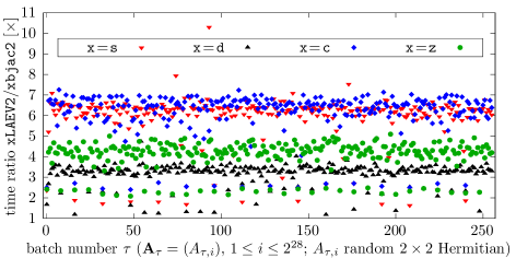
Figure 1: Batch run-time ratios of the LAPACK-based and the vectorized batched EVDs.

The EVD’s relative residual is $\rho_{A}^{\text{{x}}}=\|U\Lambda U^{\ast}-A\|_{F}/\|A\|_{F}$, where $\text{{x}}\in\{\text{{d}},\text{{z}},\text{{s}},\text{{c}}\}$ for the batched EVD in the corresponding precision and datatypes, and $\text{{x}}\in\{\text{{D}},\text{{Z}},\text{{S}},\text{{C}}\}$ for the respective LAPACK-based one. For a batch $\tau$, let $\rho_{\tau}^{\text{{x}}}=\max_{i}\rho_{A_{\tau,i}}^{\text{{x}}}$, $1\leq i\leq 2^{28}$. Then, in Fig. 2 the ratios $\rho_{\tau}^{\text{{S}}}/\rho_{\tau}^{\text{{s}}}$ and $\rho_{\tau}^{\text{{D}}}/\rho_{\tau}^{\text{{d}}}$ show that, on average, real batched EVDs are a bit more accurate than the LAPACK-based ones, but $\rho_{\tau}^{\text{{C}}}/\rho_{\tau}^{\text{{c}}}$ and $\rho_{\tau}^{\text{{Z}}}/\rho_{\tau}^{\text{{z}}}$, as indicated in Remark 2.4, demonstrate that a catastrophic loss of accuracy of the eigenvectors (which in this case are no longer of the unit norm) is possible when the components of B are of small subnormal and close enough magnitudes. If they had been (close to) normal, this issue would have been avoided. A further explanation is left for Section G.1, along with more EVD testing results. Observe that the upscaling from Eq. 18 could have preserved accuracy of the complex LAPACK routines in many problematic instances by preventing $\bar{\hbox{\tt B}}/|\hbox{\tt B}|$ to be computed with both components of similar, close to unit magnitudes. However, certain pathological cases are unavoidable even with Algorithm 2. Consider the following matrix

(30) $$A=\begin{bmatrix}\nu/8&\check{\mu}\mp\mathrm{i}\check{\mu}\\ \check{\mu}\pm\mathrm{i}\check{\mu}&\nu/8\end{bmatrix},\qquad\mathop{\mathrm{fl}}(|a_{12}|)=\check{\mu}=\mathop{\mathrm{fl}}(|a_{21}|)\implies\mathop{\mathrm{fl}}(\mathrm{e}^{\mathrm{i}\alpha})=1\pm\mathrm{i}.$$

Then, from Eq. 18, $\zeta=0$, while $\mathop{\mathrm{fl}}(\tan\varphi)=1$, $\mathop{\mathrm{fl}}(\cos\varphi)=\mathop{\mathrm{fl}}(1/\mathop{\mathrm{fl}}(\sqrt{2}))$, and therefore

$$\mathop{\mathrm{fl}}(U)=\mathop{\mathrm{fl}}(\cos\varphi)\begin{bmatrix}1&-1\pm\mathrm{i}\\ 1\pm\mathrm{i}&1\end{bmatrix},\ \ \ \det(\mathop{\mathrm{fl}}(U))\approx\frac{3}{\sqrt{2}},\ \ \ \|\mathop{\mathrm{fl}}(u_{1})\|_{F}=\|\mathop{\mathrm{fl}}(u_{2})\|_{F}\approx\frac{\sqrt{3}}{\sqrt{2}}.$$

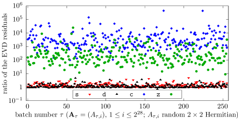
Figure 2: Per-batch ratios $\rho_{\tau}^{\text{{S}}}/\rho_{\tau}^{\text{{s}}}$, $\rho_{\tau}^{\text{{D}}}/\rho_{\tau}^{\text{{d}}}$, $\rho_{\tau}^{\text{{C}}}/\rho_{\tau}^{\text{{c}}}$, and $\rho_{\tau}^{\text{{Z}}}/\rho_{\tau}^{\text{{z}}}$ of the EVD’s relative residuals.

Neither Algorithm 2 nor ZLAEV2 can escape this miscomputing of the eigenvectors $U$ of $A$ from Eq. 30. If the strict standard conformance were not required, setting the Denormals Are Zero (DAZ) CPU flag would convert $\pm\check{\mu}$ on input to zero and the EVD of (now diagonal) $\widetilde{A}$ would be correctly computed, even with ZLAEV2, but, e.g., matrices with all subnormal elements would be zeroed out by both algorithms. If only the post-scaling subnormal values were zeroed out (e.g., by setting the Flush To Zero (FTZ) CPU flag, but not DAZ, before line 8 in Algorithm 2), then the issues with $A$ and fully subnormal matrices would vanish, but this “fix” could turn a nonsingular ill-conditioned matrix into an exactly singular one (it depends on the context if this is an issue). Thus, if the input data range is too wide for the scaling to make all matrix elements normal, it is safest to compute the EVD in a datatype with wider exponents.

5.3 The SVD results

Only a subset of the complex variant’s results is shown here, with the rest presented in Section G.2.

5.3.1 Dataset $\Xi_{1}^{\mathbb{F}}$

Figure 3 shows the speedup of $\mathtt{zvjsvd}$ versus ZGESVJ in two regimes. The max values come from comparing $\mathtt{zvjsvd}$ with the average of the corresponding run-times of ZGESVJ under full machine load, i.e., when all cores were busy running an instance of the latter on the same input at the same time. The min values are the result of a comparison with the run-times of ZGESVJ when only one instance of it was running on one core of an otherwise idle machine. For $64$ threads, e.g., the expected speedup for a given matrix order lies between the corresponding min and max values. A higher speedup might have been expected, given that both the thread-based and the vector parallelism were employed in $\mathtt{zvjsvd}$, but these results can be at least partially explained by the reasons independent of the actual hardware.

Foremost, $\mathtt{zvjsvd}$ with $\mathtt{MM}$ took $\approx\!10$ sweeps more on bigger matrices (see Fig. 15) than ZGESVJ with $\mathtt{dR}$ ($\mathtt{ME}$, where applicable, lowered the difference by $1$–$2$ sweeps). This demonstrated need for better parallel strategies for pointwise one-sided methods will remain an issue even with the most optimized parallel implementations.

As Fig. 4 shows, $\mathtt{zvjsvd}$ with $64$ threads spent most of its run-time on transforming the columns ($\bigstar$) and on computing the Frobenius norms ($\spadesuit$) and the scaled dot-products ($\clubsuit$, less so if the compensated summation was left out). For $\bigstar$, the $\max$-norm approximation of the transformed columns of the iteration matrix was also computed. For $\spadesuit$, the Frobenius norms of those columns were recomputed, while ZGESVJ updated them, with a periodic recomputation [16]. The prescaling ($\heartsuit$) and the EVD ($\diamondsuit$) of the Grammians jointly took less than $2\%$ of the run-time on the bigger inputs.

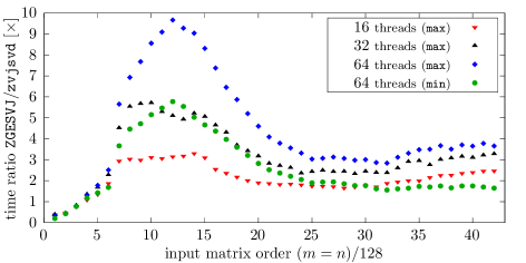
Figure 3: Run-time ratios of ZGESVJ and $\mathtt{zvjsvd}$ with $\mathtt{MM}$ on $\Xi_{1}^{\mathbb{C}}$.

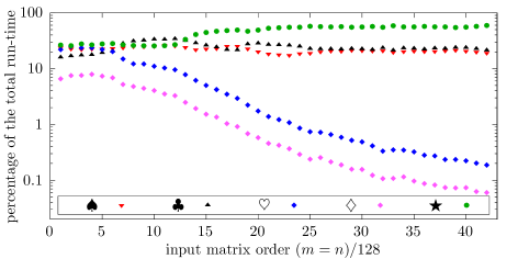
Figure 4: Breakdown of the run-time of $\mathtt{zvjsvd}$ (Algorithm 8) with $\mathtt{MM}$ on $\Xi_{1}^{\mathbb{C}}$ with $64$ threads.

Define the relative error measures $r_{G}=\|U\Sigma V^{\ast}-G\|_{F}/\|G\|_{F}$, $r_{U}=\|U^{\ast}U-I\|_{F}^{2}$, $r_{V}=\|V^{\ast}V-I\|_{F}^{2}$, and $r_{\Sigma}=\max_{j}|\sigma_{j}^{\prime}-\sigma_{j}|/|\sigma_{j}|$ for ZGESVJ, where $\sigma_{j}^{\prime}$ and $\sigma_{j}$ are the $j$th computed and exact singular value, respectively, and let $r_{G}^{\prime}$, $r_{U}^{\prime}$, $r_{V}^{\prime}$, and $r_{\Sigma}^{\prime}$ be the same measures for $\mathtt{zvjsvd}$. Figure 5 suggests that the singular values are relatively accurate and the left singular vectors are orthogonal with $\mathtt{zvjsvd}$ almost as with ZGESVJ, while the relative SVD residuals are somewhat worse, probably due to a mild ($\max_{n}{r_{V}^{\prime}}<5\cdot 10^{-20}$) loss of orthogonality of the right singular vectors. These extra errors in the proposed method might be caused by transforming $G$ and $V$ too many times (due to more sweeps) compared to ZGESVJ, by the “improper” rotations that near the end of the process lose orthogonality due to $\cos\varphi=1$ and $|\tan\varphi|\lessapprox\sqrt{\varepsilon}$.

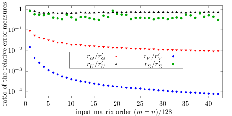
Figure 5: Ratios of the relative error measures for the SVDs on $\Xi_{1}^{\mathbb{C}}$.

5.3.2 Dataset $\Xi_{2}^{\mathbb{F}}$

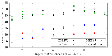
Figure 16: Number of sweeps until convergence for the LAPACK’s xGESVJ and the proposed routines (with the $\mathtt{ME}$ parallel cyclic pivot strategy), on $\Xi_{2}^{\mathbb{F}}$.

For $\Xi_{2}^{\mathbb{F}}$, $\mathtt{ME}$ was used with $\mathtt{zvjsvd}$. The MKL routines required at least $\text{{NSWEEP}}=30$ sweeps with a majority inputs (see Fig. 16). To circumvent that, z/dgesvj.f source files were taken from the LAPACK repository and modified to z/dnssvj.f, with NSWEEP as a function argument, instead of being a hard-coded parameter, what could in general benefit the users of the xGESVJ routines.

Both ZGESVJ and $\mathtt{zvjsvd}$ behaved as expected, with $r_{\Sigma}<6\cdot 10^{-2}$, $r_{\Sigma}^{\prime}<4\cdot 10^{-1}$; $r_{G}<2\cdot 10^{-14}$, $r_{G}^{\prime}<3\cdot 10^{-12}$; $\max\{r_{U},r_{U}^{\prime}\}<2\cdot 10^{-22}$; while $r_{V}<6\cdot 10^{-24}$ and $r_{V}^{\prime}<9\cdot 10^{-20}$ indicate the same problem as with $\Xi_{1}^{\mathbb{C}}$. The results were similar for $\Xi_{2}^{\mathbb{R}}$.

6 Conclusions and future work

The strongest contribution of this paper is the vectorized algorithm for the batched EVD of Hermitian matrices of order two. It requires no branching but only the basic bitwise and arithmetic operations, with $\mathrm{fma}$, and $\max$ and $\min$ that filter out a single $\mathtt{NaN}$ argument. It is not applicable if trapping on floating-point exceptions is enabled, and should be tuned for non-default rounding modes, but it is faster and often more accurate in every aspect than the matching sequence of xLAEV2 calls. Also, the computed scaled eigenvalues cannot overflow.

The proposed SVD method should be several times faster than xGESVJ on modern CPUs and scale (sublinearly) with the number of cores. A fully tuned implementation, as well as ever-increasing vector lengths on various platforms, should provide significantly better speedups, while the stored column norms could be updated as in [16]. The scaling principles from Sections 3.2, 3.4 and 4.3 cost little performance-wise, do not depend on parallelism or the pivot strategy, and thus could be incorporated into xGESVJ, as well as $\mathtt{zdpscl}^{[\prime]}$ (Algorithms 4 and 11), $\mathtt{zjrot}$ (Algorithm 7), and $\mathtt{zgsscl}$ (Algorithm 18), along with their single precision and/or real counterparts.

Appendix A Derivation and accuracy of the formulas from Section 2.1

Let $A$, $U$, and $\Lambda$ be as in Eq. 1. In Section A.1 the formulas from Section 2.1 are derived. In Section A.2 the relative errors induced while computing some of those formulas in finite precision are given as a part of the proof of Proposition 2.5.

A.1 Derivation of the formulas from Section 2.1

Equating the corresponding elements on both sides of $U^{\ast}AU=\Lambda$ and assuming $\cos\varphi\neq 0$ it follows

(31) $$\lambda_{11}/\cos^{2}\varphi =a_{11}+a_{22}\tan^{2}\varphi+2\Re\left(a_{21}\mathrm{e}^{-\mathrm{i}\alpha}\right)\tan\varphi,$$

$$\lambda_{22}/\cos^{2}\varphi =a_{11}\tan^{2}\varphi+a_{22}-2\Re\left(a_{21}\mathrm{e}^{-\mathrm{i}\alpha}\right)\tan\varphi,$$

for the diagonal elements of $\Lambda$, and

(32) $$\frac{\lambda_{21}}{\cos^{2}\varphi}\mathrm{e}^{-\mathrm{i}\alpha}=a_{21}\mathrm{e}^{-\mathrm{i}\alpha}+(a_{22}-a_{11})\tan\varphi-\bar{a}_{21}\mathrm{e}^{\mathrm{i}\alpha}\tan^{2}\varphi=0,$$

for one of the remaining off-diagonal zeros, as well as

(33) $$\frac{\lambda_{12}}{\cos^{2}\varphi}\mathrm{e}^{\mathrm{i}\alpha}=\bar{a}_{21}\mathrm{e}^{\mathrm{i}\alpha}+(a_{22}-a_{11})\tan\varphi-a_{21}\mathrm{e}^{-\mathrm{i}\alpha}\tan^{2}\varphi=0$$

for the other.

From Eq. 32 the first two, and from Eq. 33 the last two equations in

$$\bar{a}_{21}\mathrm{e}^{\mathrm{i}\alpha}\tan^{2}\varphi-a_{21}\mathrm{e}^{-\mathrm{i}\alpha}=(a_{22}-a_{11})\tan\varphi=a_{21}\mathrm{e}^{-\mathrm{i}\alpha}\tan^{2}\varphi-\bar{a}_{21}\mathrm{e}^{\mathrm{i}\alpha}$$

are obtained. Ignoring the middle equation and regrouping the terms, it follows

$$a_{21}\mathrm{e}^{-\mathrm{i}\alpha}(1+\tan^{2}\varphi)=\bar{a}_{21}\mathrm{e}^{\mathrm{i}\alpha}(1+\tan^{2}\varphi),$$

and, by canceling $1+\tan^{2}\varphi<\infty$ on both sides, $a_{21}\mathrm{e}^{-\mathrm{i}\alpha}=\bar{a}_{21}\mathrm{e}^{\mathrm{i}\alpha}$, i.e., $z=\bar{z}$, what is possible if and only if $z$ is real. Therefore,

(34) $$\alpha=\arg(a_{21}),\qquad\mathrm{e}^{\mathrm{i}\alpha}=a_{21}/|a_{21}|.$$

If $a_{21}$ is real, $\mathrm{e}^{\mathrm{i}\alpha}=\mathop{\mathrm{sign}}(a_{21})=\pm 1$.

Using Eq. 34 and $|\bar{a}_{21}|=|a_{21}|$, Eqs. 31, 32 and 33 become

$$\lambda_{11}/\cos^{2}\varphi =a_{11}+a_{22}\tan^{2}\varphi+2|a_{21}|\tan\varphi,$$

$$\lambda_{22}/\cos^{2}\varphi =a_{11}\tan^{2}\varphi+a_{22}-2|a_{21}|\tan\varphi,$$

$$\frac{\lambda_{21}}{\cos^{2}\varphi}\mathrm{e}^{-\mathrm{i}\alpha} =|a_{21}|+(a_{22}-a_{11})\tan\varphi-|a_{21}|\tan^{2}\varphi=0,$$

$$\frac{\lambda_{12}}{\cos^{2}\varphi}\mathrm{e}^{\mathrm{i}\alpha} =|a_{21}|+(a_{22}-a_{11})\tan\varphi-|a_{21}|\tan^{2}\varphi=0.$$

The last two equations above are identical, so from either one it follows

(35) $$|a_{21}|(1-\tan^{2}\varphi)=(a_{11}-a_{22})\tan\varphi.$$

If $a_{21}=0$, and since $a_{11}$ and $a_{22}$ are arbitrary, from Eq. 35 follows $\tan\varphi=0$, i.e., $U$ is the identity matrix. Else, if $a_{11}=a_{22}$, then $\tan\varphi=\pm 1$ satisfies Eq. 35. In all other cases,

$$\frac{2|a_{21}|}{a_{11}-a_{22}}=\frac{2\tan\varphi}{1-\tan^{2}\varphi}=\tan(2\varphi),$$

and, since $|\tan(2\varphi)|<\infty$, i.e., $|\varphi|<\pi/4$,

$$\tan\varphi=\frac{\tan(2\varphi)}{1+\sqrt{1+\tan^{2}(2\varphi)}}.$$

A.1.1 Proof of Lemma 2.1

See the main paper for its statement.

Proof A.1.

Observe that $m$ and $M$ in Eq. 13 are exact, being normal or not, so any underflow in their formation is harmless. A possible underflow of $\mathop{\mathrm{fl}}(q)$ is harmless as well. If $\mathop{\mathrm{fl}}(q)$ is subnormal or zero, $\mathop{\mathrm{fma}}(\mathop{\mathrm{fl}}(q),\mathop{\mathrm{fl}}(q),1)=\mathop{\mathrm{fma}}(q,q,1)$, as if $\varepsilon_{1}=0$ below.

Let $\mathop{\mathrm{fl}}(q)=q(1+\varepsilon_{1})$, where $|\varepsilon_{1}|\leq\varepsilon$. Then,

$$\mathop{\mathrm{fl}}((\mathop{\mathrm{fl}}(q))^{2}+1)=\mathop{\mathrm{fma}}(\mathop{\mathrm{fl}}(q),\mathop{\mathrm{fl}}(q),1)=(q^{2}(1+\varepsilon_{1})^{2}+1)(1+\varepsilon_{3})=r(1+\varepsilon_{3}),$$

where $|\varepsilon_{3}|\leq\varepsilon$. Expressing $r$ as the wanted, exact quantity times a relative error factor, $r=(q^{2}+1)(1+\varepsilon_{2})$, and solving this equation for $\varepsilon_{2}$, it follows

$$\varepsilon_{2}=\frac{q^{2}}{q^{2}+1}\varepsilon_{1}(2+\varepsilon_{1}).$$

Since $0\leq q\leq 1$, the fraction above ranges from $0$ (for $q=0$) to $1/2$ (for $q=1$), inclusive, irrespectively of $\varepsilon_{1}$. Therefore, $\varepsilon_{2}$, as a function of $\varepsilon_{1}$ when $q=1$, attains the extremal values for $\varepsilon_{1}=\mp\varepsilon$,

$$-\frac{\varepsilon(2-\varepsilon)}{2}\leq\frac{1}{2}\varepsilon_{1}(2+\varepsilon_{1})\leq\frac{\varepsilon(2+\varepsilon)}{2}.$$

However, if $q=1$ (equivalently, if $m=M$), then $\varepsilon_{1}=0$ since the division is exact, and the two inequalities above are in fact strict, i.e., neither equality is possible.

Now, $\mathop{\mathrm{fl}}(\sqrt{\mathop{\mathrm{fma}}(\mathop{\mathrm{fl}}(q),\mathop{\mathrm{fl}}(q),1)})=\sqrt{(q^{2}+1)(1+\varepsilon_{2})(1+\varepsilon_{3})}(1+\varepsilon_{4})$, where $|\varepsilon_{4}|\leq\varepsilon$. The final multiplication by $M$ gives, with $|\varepsilon_{5}|\leq\varepsilon$,

$$\mathop{\mathrm{fl}}(\mathop{\mathrm{hypot}}(x,y))=M\sqrt{q^{2}+1}\sqrt{1+\varepsilon_{2}}\sqrt{1+\varepsilon_{3}}(1+\varepsilon_{4})(1+\varepsilon_{5})=\delta_{2}\mathop{\mathrm{hypot}}(x,y),$$

where $\delta_{2}=\sqrt{1+\varepsilon_{2}}\sqrt{1+\varepsilon_{3}}(1+\varepsilon_{4})(1+\varepsilon_{5})$ is minimized for $\varepsilon_{3}=\varepsilon_{4}=\varepsilon_{5}=-\varepsilon$ and $\varepsilon_{2}=-\varepsilon(2-\varepsilon)/2$, and maximized for $\varepsilon_{3}=\varepsilon_{4}=\varepsilon_{5}=\varepsilon$ and $\varepsilon_{2}=\varepsilon(2+\varepsilon)/2$.

Remark A.2.

When considering relative floating-point accuracy of a computation, any underflow by itself, in isolation, is harmless if the result is exact, since the relative error is zero. But it is too cumbersome to always state this obvious exception.

A.2 Proof of Proposition 2.5

See the main paper for its statement.

Proof A.3.

If $a_{21}$ is real, $\mathop{\mathrm{fl}}(|a_{21}|)=\delta_{o}^{\mathbb{R}}|a_{21}|$, $\delta_{o}^{\mathbb{R}}=1$, else $\mathop{\mathrm{fl}}(|a_{21}|)=\delta_{o}^{\mathbb{C}}|a_{21}|$, where $\delta_{o}^{\mathbb{C}}=\delta_{2}$ (see Lemma 2.1). Thus, in the complex case, from Eq. 4 it follows

$$\mathop{\mathrm{fl}}(\cos\alpha)=\cos\alpha\frac{1+\varepsilon_{1}}{\delta_{2}}=\delta_{\alpha}^{\prime}\cos\alpha,\qquad\mathop{\mathrm{fl}}(\sin\alpha)=\sin\alpha\frac{1+\varepsilon_{2}}{\delta_{2}}=\delta_{\alpha}^{\prime\prime}\sin\alpha,$$

where $\max\{|\varepsilon_{1}|,|\varepsilon_{2}|\}\leq\varepsilon$. The error factors $\delta_{\alpha}^{\prime}$ and $\delta_{\alpha}^{\prime\prime}$ are maximized for $\varepsilon_{1}=\varepsilon_{2}=\varepsilon$ and $\delta_{2}=\delta_{2}^{-}$, and minimized for $\varepsilon_{1}=\varepsilon_{2}=-\varepsilon$ and $\delta_{2}=\delta_{2}^{+}$. Let $\delta_{\alpha}^{+}=(1+\varepsilon)/\delta_{2}^{-}$ and $\delta_{\alpha}^{-}=(1-\varepsilon)/\delta_{2}^{+}$. Since $\min\{|x|,|y|\}\leq\sqrt{x^{2}\cos^{2}\alpha+y^{2}\sin^{2}\alpha}\leq\max\{|x|,|y|\}$,

(36) $$1-4.000000\,\varepsilon\lessapprox\delta_{\alpha}^{-}<|\mathop{\mathrm{fl}}(\mathrm{e}^{\pm\mathrm{i}\alpha})|<\delta_{\alpha}^{+}\lessapprox 1+4.000001\,\varepsilon.$$

The approximated multiples of $\varepsilon$ come from evaluating $(1-\delta_{\alpha}^{-})/\varepsilon$ and $(\delta_{\alpha}^{+}-1)/\varepsilon$, as explained for Eqs. 42 and 43 below.

From Eq. 6, $\mathop{\mathrm{fl}}(|a|)=|a_{11}-a_{22}|(1+\varepsilon_{3})$, where $|\varepsilon_{3}|\leq\varepsilon$, and $\mathop{\mathrm{fl}}(2|a_{21}|)=2\mathop{\mathrm{fl}}(|a_{21}|)$. First, assume that $\mathop{\mathrm{fl}}(2|a_{21}|/|a|)\leq\mathop{\mathrm{fl}}(\sqrt{\nu})$. Then,

$$\mathop{\mathrm{fl}}(\tan 2\varphi)=\mathop{\mathrm{fl}}(2|a_{21}|/|a|)\mathop{\mathrm{sign}}{a}=\delta_{2\varphi}^{\mathbb{F}}(2|a_{21}|/|a|)\mathop{\mathrm{sign}}{a}=\delta_{2\varphi}^{\mathbb{F}}\tan 2\varphi,$$

where $\delta_{2\varphi}^{\mathbb{C}}=\delta_{2}/(1+\varepsilon_{3})$ and $\delta_{2\varphi}^{\mathbb{R}}=1/(1+\varepsilon_{3})$. Minimizing and maximizing these fractions, similarly as above, it follows

(37) $$\begin{gathered}\delta_{2\varphi}^{\mathbb{C}-}=\frac{\delta_{2}^{-}}{1+\varepsilon}<\delta_{2\varphi}^{\mathbb{C}}<\frac{\delta_{2}^{+}}{1-\varepsilon}=\delta_{2\varphi}^{\mathbb{C}+},\\ \delta_{2\varphi}^{\mathbb{R}-}=\frac{1}{1+\varepsilon}\leq\delta_{2\varphi}^{\mathbb{R}}\leq\frac{1}{1-\varepsilon}=\delta_{2\varphi}^{\mathbb{R}+}.\end{gathered}$$

Else, let $\nu\geq\mathop{\mathrm{fl}}(2|a_{21}|/|a|)>\mathop{\mathrm{fl}}(\sqrt{\nu})$ and assume that $|\mathop{\mathrm{fl}}(\tan 2\varphi)|$ was not bounded above by $\mathop{\mathrm{fl}}(\sqrt{\nu})$. Then $|\mathop{\mathrm{fl}}(\tan\varphi)|$ would have been the exact unity if the square root in Eq. 5 was computed as finite, e.g., using $\mathop{\mathrm{hypot}}(1,\mathop{\mathrm{fl}}(\tan 2\varphi))$ and assuming

$$|x|\geq\mathop{\mathrm{fl}}(\sqrt{\nu})\implies\mathop{\mathrm{hypot}}(1,x)=|x|\ \wedge\ 1+|x|=|x|$$

for a representable $x$. Therefore, regardless of the relative error in $\mathop{\mathrm{fl}}(\tan 2\varphi)$, the relative error in $\mathop{\mathrm{fl}}(\tan\varphi)$ could have only decreased in magnitude from the one obtained with $\mathop{\mathrm{fl}}(\tan 2\varphi)=\mathop{\mathrm{fl}}(\sqrt{\nu})$, when also $|\mathop{\mathrm{fl}}(\tan\varphi)|=1$, since $\tan\varphi\to\pm 1$ monotonically for $\tan 2\varphi\to\pm\infty$. The Jacobi rotation is built from $\mathop{\mathrm{fl}}(\tan\varphi)$ (and the functions of $\alpha$ in the complex case), while $\mathop{\mathrm{fl}}(\tan 2\varphi)$ is just an intermediate result and thus the relative error in it is not relevant as long as the one in $\mathop{\mathrm{fl}}(\tan\varphi)$ is kept in check.

By substituting $\mathop{\mathrm{fl}}(\tan 2\varphi)$ for $\tan 2\varphi$ in Eq. 5 and using the fused multiply-add for the argument of the square root, with $\max\{|\varepsilon_{4}|,|\varepsilon_{5}|,|\varepsilon_{6}|,|\varepsilon_{7}|\}\leq\varepsilon$ it follows that

(38) $$\mathop{\mathrm{fl}}(\tan\varphi)=\frac{\delta_{2\varphi}^{\mathbb{F}}\tan 2\varphi(1+\varepsilon_{7})}{(1+\sqrt{((\delta_{2\varphi}^{\mathbb{F}}\tan 2\varphi)^{2}+1)(1+\varepsilon_{4})}(1+\varepsilon_{5}))(1+\varepsilon_{6})}=\delta_{\varphi}^{\mathbb{F}}\tan\varphi,$$

where $\varepsilon_{4}$, $\varepsilon_{5}$, $\varepsilon_{6}$, and $\varepsilon_{7}$ stand for the relative rounding errors of the $\mathrm{fma}$, the square root, the addition of one, and the division, respectively, and $\delta_{\varphi}^{\mathbb{F}}$ remains to be bounded.

Let $y=\tan 2\varphi$. From Eq. 38, by solving the equation

$$(\delta_{2\varphi}^{\mathbb{F}})^{2}y^{2}+1=(y^{2}+1)(1+x)$$

for $x$, it is possible to express the relative error present in the intermediate result of the $\mathrm{fma}$ before its rounding, as a function of $\varphi$ (due to $y$) and $\varepsilon$ (due to $(\delta_{2\varphi}^{\mathbb{F}})^{2}$),

(39) $$x=\frac{y^{2}}{y^{2}+1}\varepsilon_{2\varphi}^{\mathbb{F}},\qquad\varepsilon_{2\varphi}^{\mathbb{F}}=(\delta_{2\varphi}^{\mathbb{F}})^{2}-1,\qquad 0\leq|x|<|\varepsilon_{2\varphi}^{\mathbb{F}}|,$$

since $0\leq y^{2}/(y^{2}+1)<1$ for all $y$. From Eq. 37 $\varepsilon_{2\varphi}^{\mathbb{F}}$, and thus $x$, can be bounded as

(40) $$(\delta_{2\varphi}^{\mathbb{F}-})^{2}-1=\varepsilon_{2\varphi}^{\mathbb{F}-}\leq\varepsilon_{2\varphi}^{\mathbb{F}}\leq\varepsilon_{2\varphi}^{\mathbb{F}+}=(\delta_{2\varphi}^{\mathbb{F}+})^{2}-1.$$

By rewriting the fma operation as above, Eq. 38 can be expressed as

$$\mathop{\mathrm{fl}}(\tan\varphi)=\frac{\tan 2\varphi}{1+\sqrt{\tan^{2}2\varphi+1}\sqrt{1+x}\sqrt{1+\varepsilon_{4}}(1+\varepsilon_{5})}\frac{\delta_{2\varphi}^{\mathbb{F}}(1+\varepsilon_{7})}{1+\varepsilon_{6}},$$

or, letting $r=\sqrt{\tan^{2}2\varphi+1}$, $b=\sqrt{1+x}\sqrt{1+\varepsilon_{4}}(1+\varepsilon_{5})$, and $b^{\prime}=\delta_{2\varphi}^{\mathbb{F}}(1+\varepsilon_{7})/(1+\varepsilon_{6})$,

$$\mathop{\mathrm{fl}}(\tan\varphi)=\frac{\tan 2\varphi}{1+br}b^{\prime}=\frac{\tan 2\varphi}{(1+r)(1+d)}b^{\prime}=\tan\varphi\frac{b^{\prime}}{1+d}=\delta_{\varphi}^{\mathbb{F}}\tan\varphi,\qquad r\geq 1.$$

Similarly as before, the equation $1+br=(1+r)(1+d)$ has to be solved for $d$ to factor out the relative error (i.e., $d$) from the remaining exact value (i.e., $1+r$). Then,

(41) $$d=\frac{r}{r+1}(b-1),\quad\frac{|b-1|}{2}\leq|d|<|b-1|,\quad\delta_{\varphi}^{\mathbb{F}}=\frac{\delta_{2\varphi}^{\mathbb{F}}(1+\varepsilon_{7})}{(1+d)(1+\varepsilon_{6})}.$$

Maximizing $|\delta_{\varphi}^{\mathbb{F}}|=\delta_{\varphi}^{\mathbb{F}}$ is equivalent to maximizing $|\delta_{2\varphi}^{\mathbb{F}}|=\delta_{2\varphi}^{\mathbb{F}}$ as $\delta_{2\varphi}^{\mathbb{F}+}$ from Eq. 37 and minimizing $d$, while setting $\varepsilon_{6}=-\varepsilon$ and $\varepsilon_{7}=\varepsilon$. Minimizing $d$ is equivalent to letting $r\to\infty$ in Eq. 41 and minimizing $b$, what amounts to setting $\varepsilon_{4}=\varepsilon_{5}=-\varepsilon$ and minimizing $x$ by letting $y^{2}\to\infty$ in Eq. 39 and taking $\varepsilon_{2\varphi}^{\mathbb{F}-}$ from Eq. 40 as the limiting value. Therefore, the maximal value of $\delta_{\varphi}^{\mathbb{F}}$ is bounded above as

(42) $$\max\delta_{\varphi}^{\mathbb{F}}<\hat{\delta}_{\varphi}^{\mathbb{F}}=\frac{\delta_{2\varphi}^{\mathbb{F}+}(1+\varepsilon)}{\sqrt{1+\varepsilon_{2\varphi}^{\mathbb{F}-}}(1-\varepsilon)^{5/2}}\lessapprox\begin{cases}1+\hphantom{0}5.500001\,\varepsilon,&\mathbb{F}=\mathbb{R},\\ 1+11.500004\,\varepsilon,&\mathbb{F}=\mathbb{C}.\end{cases}$$

First, $(\hat{\delta}_{\varphi}^{\mathbb{F}}-1)/\varepsilon$, i.e., the factors multiplying $\varepsilon$ above, were expressed as functions of $\varepsilon$ in the scripts from Section A.3. The factors were symbolically computed for $\varepsilon\in\{2^{-11},2^{-24},2^{-53},2^{-113}\}$, evaluated with $50$ digits of precision, manually rounded upwards to six decimal places, and the maximums over $p\in\{23,52,112\}$ were taken.

Minimizing $\delta_{\varphi}^{\mathbb{F}}$ is equivalent to minimizing $\delta_{2\varphi}^{\mathbb{F}}$ as $\delta_{2\varphi}^{\mathbb{F}-}$ from Eq. 37 and maximizing $d$, while setting $\varepsilon_{6}=\varepsilon$ and $\varepsilon_{7}=-\varepsilon$. Maximizing $d$ is equivalent to letting $r\to\infty$ in Eq. 41 and maximizing $b$, what amounts to setting $\varepsilon_{4}=\varepsilon_{5}=\varepsilon$ and maximizing $x$ by letting $y^{2}\to\infty$ in Eq. 39 and taking $\varepsilon_{2\varphi}^{\mathbb{F}+}$ from Eq. 40 as the limiting value. Therefore, the minimal value of $\delta_{\varphi}^{\mathbb{F}}$ is bounded below (the factors multiplying $\varepsilon$ come from $(1-\check{\delta}_{\varphi}^{\mathbb{F}})/\varepsilon$), as

(43) $$\min\delta_{\varphi}^{\mathbb{F}}>\check{\delta}_{\varphi}^{\mathbb{F}}=\frac{\delta_{2\varphi}^{\mathbb{F}-}(1-\varepsilon)}{\sqrt{1+\varepsilon_{2\varphi}^{\mathbb{F}+}}(1+\varepsilon)^{5/2}}\gtrapprox\begin{cases}1-\hphantom{0}5.500000\,\varepsilon,&\quad\mathbb{F}=\mathbb{R},\\ 1-11.500000\,\varepsilon,&\quad\mathbb{F}=\mathbb{C}.\end{cases}$$

Due to monotonicity of all arithmetic operations involved in computing $\mathop{\mathrm{fl}}(\tan\varphi)$, its absolute value cannot exceed unity, regardless of $\delta_{\varphi}^{\mathbb{F}}$. Therefore, the magnitude of (either component of) $\mathrm{e}^{\prime}=\mathop{\mathrm{fl}}(\mathrm{e}^{\mathrm{i}\alpha})\mathop{\mathrm{fl}}(\tan\varphi)$ cannot increase from that of (the corresponding component of) $\mathop{\mathrm{fl}}(\mathrm{e}^{\mathrm{i}\alpha})$ after its multiplication by $\mathop{\mathrm{fl}}(\tan\varphi)$.

From Eqs. 5, 7 and 10 it follows

(44) $$\mathop{\mathrm{fl}}(\cos\varphi)=\frac{\delta_{1}}{\sqrt{((\delta_{\varphi}^{\mathbb{F}})^{2}\tan^{2}\varphi+1)(1+\varepsilon_{8})}}.$$

As done previously, let $t=\tan\varphi$ and solve $(\delta_{\varphi}^{\mathbb{F}})^{2}t^{2}+1=(t^{2}+1)(1+c)$ for $c$, to get

(45) $$c=\frac{t^{2}}{t^{2}+1}\varepsilon_{\varphi}^{\mathbb{F}},\qquad\varepsilon_{\varphi}^{\mathbb{F}}=(\delta_{\varphi}^{\mathbb{F}})^{2}-1,\qquad 0\leq|c|<|\varepsilon_{\varphi}^{\mathbb{F}}|,$$

and re-express Eq. 44, with $|\varepsilon_{8}|\leq\varepsilon$ coming from the $\mathrm{fma}$’s rounding, as

(46) $$\mathop{\mathrm{fl}}(\cos\varphi)=\frac{1}{\sqrt{\tan^{2}\varphi+1}}\frac{\delta_{1}}{\sqrt{1+c}\sqrt{1+\varepsilon_{8}}}=\delta_{c}^{\mathbb{F}}\cos\varphi.$$

Maximizing $|\delta_{c}^{\mathbb{F}}|=\delta_{c}^{\mathbb{F}}$ amounts to setting $\varepsilon_{8}=-\varepsilon$ and $\delta_{1}=\delta_{1}^{+}$, while minimizing $c$ by letting $t^{2}\to\infty$ in Eq. 45 and taking $\check{\varepsilon}_{\varphi}^{\mathbb{F}}=(\check{\delta}_{\varphi}^{\mathbb{F}})^{2}-1$ as the limiting value. Therefore,

(47) $$\max\delta_{c}^{\mathbb{F}}<\hat{\delta}_{c}^{\mathbb{F}}=\frac{\delta_{1}^{+}}{\sqrt{1+\check{\varepsilon}_{\varphi}^{\mathbb{F}}}\sqrt{1-\varepsilon}}\lessapprox\begin{cases}1+\hphantom{0}8.000002\,\varepsilon,&\mathbb{F}=\mathbb{R},\\ 1+14.000006\,\varepsilon,&\mathbb{F}=\mathbb{C}.\end{cases}$$

Minimizing $\delta_{c}^{\mathbb{F}}$ amounts to setting $\varepsilon_{8}=\varepsilon$ and $\delta_{1}=\delta_{1}^{-}$, while maximizing $c$ by letting $t^{2}\to\infty$ in Eq. 45 and taking $\hat{\varepsilon}_{\varphi}^{\mathbb{F}}=(\hat{\delta}_{\varphi}^{\mathbb{F}})^{2}-1$ as the limiting value. Therefore,

(48) $$\min\delta_{c}^{\mathbb{F}}>\check{\delta}_{c}^{\mathbb{F}}=\frac{\delta_{1}^{-}}{\sqrt{1+\hat{\varepsilon}_{\varphi}^{\mathbb{F}}}\sqrt{1+\varepsilon}}\gtrapprox\begin{cases}1-\hphantom{0}8.000000\,\varepsilon,&\mathbb{F}=\mathbb{R},\\ 1-14.000000\,\varepsilon,&\mathbb{F}=\mathbb{C}.\end{cases}$$

The floating-point arithmetic operations involved in computing $\mathop{\mathrm{fl}}(\cos\varphi)$ are monotonic, so $0\leq\mathop{\mathrm{fl}}(\cos\varphi)\leq 1$ regardless of $\delta_{c}^{\mathbb{F}}$.

Computation of the eigenvalues proceeds, with $o=2|a_{21}|$ and $\tilde{o}=\delta_{o}^{\mathbb{F}}o$, as

(49) $$\mathop{\mathrm{fl}}(\lambda_{1}^{\prime}) =\mathop{\mathrm{fma}}(\mathop{\mathrm{fma}}(a_{22},\tilde{t},\hphantom{-}\tilde{o}),\tilde{t},a_{11}),$$

$$\mathop{\mathrm{fl}}(\lambda_{2}^{\prime}) =\mathop{\mathrm{fma}}(\mathop{\mathrm{fma}}(a_{11},\tilde{t},-\tilde{o}),\tilde{t},a_{22}),$$

where $\tilde{t}=\mathop{\mathrm{fl}}(\tan\varphi)$ and $|\tilde{t}|\leq 1$. Then, with $\max\{|\varepsilon_{10}|,|\varepsilon_{11}|,|\varepsilon_{12}|,|\varepsilon_{13}|\}\leq\varepsilon$,

$$\mathop{\mathrm{fl}}(\lambda_{1}^{\prime}) =((a_{22}\tilde{t}+\tilde{o})(1+\varepsilon_{10})\tilde{t}+a_{11})(1+\varepsilon_{12}),$$

$$\mathop{\mathrm{fl}}(\lambda_{2}^{\prime}) =((a_{11}\tilde{t}-\tilde{o})(1+\varepsilon_{11})\tilde{t}+a_{22})(1+\varepsilon_{13}),$$

what gives, after taking the absolute values, applying the triangle inequality, and using Eq. 15 to bound $|a_{ij}|$ from above, with $\hat{\delta}_{o}^{\mathbb{R}}=1$ and $\hat{\delta}_{o}^{\mathbb{C}}=\delta_{2}^{+}$,

(50) $$|\mathop{\mathrm{fl}}(\lambda^{\prime})|\leq((\hat{a}+2\hat{a}\hat{\delta}_{o}^{\mathbb{F}})(1+\varepsilon)+\hat{a})(1+\varepsilon)=\hat{a}((1+2\hat{\delta}_{o}^{\mathbb{F}})(1+\varepsilon)+1)(1+\varepsilon),$$

where $|\mathop{\mathrm{fl}}(\lambda^{\prime})|=\max\{|\mathop{\mathrm{fl}}(\lambda_{1}^{\prime})|,|\mathop{\mathrm{fl}}(\lambda_{2}^{\prime})|\}$. Bounding $\hat{a}$ by $\tilde{\nu}$ as in Eq. 15 gives

$$|\mathop{\mathrm{fl}}(\lambda^{\prime})|\leq\tilde{\nu}((1+2\hat{\delta}_{o}^{\mathbb{F}})(1+\varepsilon)+1)(1+\varepsilon)=\tilde{\nu}\delta_{\mathbb{F}}^{\prime}.$$

Evaluating the scripts from Section A.3 for all $\varepsilon$ considered above shows that $4<\delta_{\mathbb{F}}^{\prime}\ll 4\sqrt{2}\gtrapprox 5.656854$, so $|\mathop{\mathrm{fl}}(\lambda^{\prime})|<\nu$.

Since $\mathop{\mathrm{fl}}(\sec^{2}\varphi)\geq 1$, dividing $\mathop{\mathrm{fl}}(\lambda_{1}^{\prime})$ and $\mathop{\mathrm{fl}}(\lambda_{2}^{\prime})$ by it therefore cannot raise their magnitudes, and the final computed eigenvalues cannot overflow—thus far, with the assumption that no final result of any previous computation has underflowed.

Regardless of the consequences of any underflow leading to $\tilde{t}$, $|\tilde{t}|\leq 1$ in Eq. 49 due to Eq. 5, and $|\mathop{\mathrm{fl}}(\lambda^{\prime})|$ can be bounded above, with $a_{2}^{1}=\max\{|a_{11}|,|a_{22}|\}\leq\tilde{\nu}$, by

(51) $$((a_{2}^{1}+\tilde{o})(1+\varepsilon)+a_{2}^{1})(1+\varepsilon),$$

similarly as in Eq. 50, letting in both inequalities $\tilde{t}=1$. If $a_{2}^{1}$ and $\tilde{o}$ are small, no overflow occurs. If $a_{2}^{1}$ is large enough, a small enough $\tilde{o}$, no matter if accurate or not, cannot affect it by addition or subtraction in the default rounding mode, so Eq. 51 becomes $a_{2}^{1}(2+\varepsilon)(1+\varepsilon)$. Vice versa, a small enough $a_{2}^{1}$ cannot affect a large enough $\tilde{o}$, so Eq. 51 simplifies to $\tilde{o}(1+\varepsilon)^{2}$. No overflow is possible in either case.

A.3 The Wolfram Language scripts used in Section A.2

These scripts were executed by the Wolfram Language Engine, version 12.3.1 for macOS.

A.3.1 A script computing the relative error bounds for a real $A$

In Fig. 6, n is the number of digits of precision for N[…], and

$$\text{{fem}}=(1-\check{\delta}_{\varphi}^{\mathbb{R}})/\varepsilon,\ \ \ \text{{fep}}=(\hat{\delta}_{\varphi}^{\mathbb{R}}-1)/\varepsilon,\ \ \ \text{{cem}}=(1-\check{\delta}_{c}^{\mathbb{R}})/\varepsilon,\ \ \ \text{{cep}}=(\hat{\delta}_{c}^{\mathbb{R}}-1)/\varepsilon,\ \ \ \text{{pel}}=\delta_{\mathbb{R}}^{\prime}.$$

#!/usr/bin/env wolframscript -print all
If[Length[$ScriptCommandLine]<3,Quit[]];
p=ToExpression[$ScriptCommandLine[[2]]];
n=ToExpression[$ScriptCommandLine[[3]]];
p1=-p-1; (* change p1 to -p if rounding is not to the nearest *)
p2=2^p1;
d1m[e_]:=(1-e)/(1+e); (* \delta_1^- *)
d1p[e_]:=(1+e)/(1-e); (* \delta_1^+ *)
dam[e_]:=1;
dap[e_]:=1;
ddm[e_]:=1/(1+e);
ddp[e_]:=1/(1-e);
edm[e_]:=(ddm[e])^2-1;
edp[e_]:=(ddp[e])^2-1;
dfm[e_]:=(ddm[e]*(1-e))/(Sqrt[1+edp[e]]*((1+e)^(5/2)));
dfp[e_]:=(ddp[e]*(1+e))/(Sqrt[1+edm[e]]*((1-e)^(5/2)));
fem[e_]:=(1-dfm[e])/e;
fep[e_]:=(dfp[e]-1)/e;
"fem="<>ToString[N[FullSimplify[fem[p2]],n]]
"fep="<>ToString[N[FullSimplify[fep[p2]],n]]
efm[e_]:=dfm[e]^2-1;
efp[e_]:=dfp[e]^2-1;
dcm[e_]:=d1m[e]/(Sqrt[1+efp[e]]*Sqrt[1+e]);
dcp[e_]:=d1p[e]/(Sqrt[1+efm[e]]*Sqrt[1-e]);
cem[e_]:=(1-dcm[e])/e;
cep[e_]:=(dcp[e]-1)/e;
"cem="<>ToString[N[FullSimplify[cem[p2]],n]]
"cep="<>ToString[N[FullSimplify[cep[p2]],n]]
pel[e_]:=(3*(1+e)+1)*(1+e);
"pel="<>ToString[N[FullSimplify[pel[p2]],n]]

Figure 6: A script computing the relative error bounds for a real $A$ in Proposition 2.5.

A.3.2 A script computing the relative error bounds for a complex $A$

In Fig. 7, n is the number of digits of precision for N[…], and

$$\begin{gathered}\text{{fam}}=(1-\delta_{\alpha}^{-})/\varepsilon,\quad\text{{fap}}=(\delta_{\alpha}^{+}-1)/\varepsilon,\\ \text{{fem}}=(1-\check{\delta}_{\varphi}^{\mathbb{C}})/\varepsilon,\ \text{{fep}}=(\hat{\delta}_{\varphi}^{\mathbb{C}}-1)/\varepsilon,\ \text{{cem}}=(1-\check{\delta}_{c}^{\mathbb{C}})/\varepsilon,\ \text{{cep}}=(\hat{\delta}_{c}^{\mathbb{C}}-1)/\varepsilon,\ \text{{pel}}=\delta_{\mathbb{C}}^{\prime}.\end{gathered}$$

#!/usr/bin/env wolframscript -print all
If[Length[$ScriptCommandLine]<3,Quit[]];
p=ToExpression[$ScriptCommandLine[[2]]];
n=ToExpression[$ScriptCommandLine[[3]]];
p1=-p-1; (* change p1 to -p if rounding is not to the nearest *)
p2=2^p1;
d1m[e_]:=(1-e)/(1+e); (* \delta_1^- *)
d1p[e_]:=(1+e)/(1-e); (* \delta_1^+ *)
d2m[e_]:=((1-e)^(5/2))*Sqrt[1-(e*(2-e))/2]; (* \delta_2^- *)
d2p[e_]:=((1+e)^(5/2))*Sqrt[1+(e*(2+e))/2]; (* \delta_2^+ *)
dam[e_]:=(1-e)/d2p[e];
dap[e_]:=(1+e)/d2m[e];
fam[e_]:=(1-dam[e])/e;
fap[e_]:=(dap[e]-1)/e;
"fam="<>ToString[N[FullSimplify[fam[p2]],n]]
"fap="<>ToString[N[FullSimplify[fap[p2]],n]]
ddm[e_]:=d2m[e]/(1+e);
ddp[e_]:=d2p[e]/(1-e);
edm[e_]:=(ddm[e])^2-1;
edp[e_]:=(ddp[e])^2-1;
dfm[e_]:=(ddm[e]*(1-e))/(Sqrt[1+edp[e]]*((1+e)^(5/2)));
dfp[e_]:=(ddp[e]*(1+e))/(Sqrt[1+edm[e]]*((1-e)^(5/2)));
fem[e_]:=(1-dfm[e])/e;
fep[e_]:=(dfp[e]-1)/e;
"fem="<>ToString[N[FullSimplify[fem[p2]],n]]
"fep="<>ToString[N[FullSimplify[fep[p2]],n]]
efm[e_]:=dfm[e]^2-1;
efp[e_]:=dfp[e]^2-1;
dcm[e_]:=d1m[e]/(Sqrt[1+efp[e]]*Sqrt[1+e]);
dcp[e_]:=d1p[e]/(Sqrt[1+efm[e]]*Sqrt[1-e]);
cem[e_]:=(1-dcm[e])/e;
cep[e_]:=(dcp[e]-1)/e;
"cem="<>ToString[N[FullSimplify[cem[p2]],n]]
"cep="<>ToString[N[FullSimplify[cep[p2]],n]]
pel[e_]:=((1+2*d2p[e])*(1+e)+1)*(1+e);
"pel="<>ToString[N[FullSimplify[pel[p2]],n]]
(* for Lemma 3.2 only *)
eps[e_]:=FullSimplify[e*(2+dap[e])+(e^2)*(1+dap[e])];
"eps="<>ToString[N[FullSimplify[eps[p2]/p2],n]]
epp[e_]:=FullSimplify[Sqrt[2]*(eps[e]*(1+e)+e)];
"epp="<>ToString[N[FullSimplify[epp[p2]/p2],n]]

Figure 7: A script computing the relative error bounds for a complex $A$ in Proposition 2.5.

Appendix B Several vectorized routines mentioned in the main paper

B.1 Vectorized eigendecomposition of a batch of real symmetric matrices of order two

Algorithms 9 and 10 are the real counterparts of Algorithms 2 and 3. The complex algorithms work also with real symmetric matrices on input as a special case, but the real ones are faster. The real algorithms return $\pm\tan\varphi=\mathrm{e}^{\mathrm{i}\alpha}\tan\varphi=\mathop{\mathrm{sign}}a_{21}\tan\varphi$, as the complex ones do with a real input.

Algorithm 9 $\mathtt{d8jac2}$: a vectorized eigendecomposition of at most $\mathtt{s}$ double precision real symmetric matrices of order two with the Intel’s AVX-512 intrinsics.

0:  $\mathtt{i}$; addresses of $\tilde{\mathbf{a}}_{11},\tilde{\mathbf{a}}_{22},\tilde{\mathbf{a}}_{21},\pm\tan\tilde{\bm{\varphi}},\cos\tilde{\bm{\varphi}},\tilde{\bm{\lambda}}_{1},\tilde{\bm{\lambda}}_{2},\tilde{\mathtt{p}}$

0:  $\pm\mathop{\mathsf{tan}}\varphi$, $\mathop{\mathsf{cos}}\varphi$; $\bm{\lambda}_{1}$, $\bm{\lambda}_{2}$; $\mathfrak{p}$ /​/ a permutation-indicating bitmask/​/ vectors with all lanes set to a compile-time constant

1:  $\mathsf{0}=\mathop{\mathtt{setzero}}();\quad\mathsf{1}=\mathop{\mathtt{set1}}(1.0);\quad-\mathsf{0}=\mathop{\mathtt{set1}}(-0.0);\quad\bm{\nu}=\mathop{\mathtt{set1}}(\mathtt{DBL\_MAX});$

2:  $\sqrt{\bm{\nu}}=\mathop{\mathtt{set1}}(\text{{1.34078079299425956E+154}});\quad\bm{\eta}=\mathop{\mathtt{set1}}(1020.0);$ /​/ $\mathop{\mathrm{fl}}(\sqrt{\nu})$: Eq. 6/​/ aligned loads of the $\mathtt{i}$th input vectors

3:  $\mathsf{a}_{11}=\mathop{\mathtt{load}}(\tilde{\mathbf{a}}_{11}+\mathtt{i});\quad\mathsf{a}_{22}=\mathop{\mathtt{load}}(\tilde{\mathbf{a}}_{22}+\mathtt{i});\quad\mathsf{a}_{21}=\mathop{\mathtt{load}}(\tilde{\mathbf{a}}_{21}+\mathtt{i});$ /​/ $\Im{a_{21}}=0$/​/ the scaling exponents $\bm{\zeta}$;   lane-wise $\mathop{\mathrm{getexp}}(x)=\left\lfloor\lg|x|\right\rfloor,\left\lfloor\lg 0\right\rfloor=-\infty$

4:  $\bm{\zeta}_{11}\mskip-2.0mu=\mskip-2.0mu\mathop{\mathtt{sub}}(\bm{\eta},\mathop{\mathtt{getexp}}(\mathsf{a}_{11}));\mskip 3.5mu\bm{\zeta}_{22}\mskip-2.0mu=\mskip-2.0mu\mathop{\mathtt{sub}}(\bm{\eta},\mathop{\mathtt{getexp}}(\mathsf{a}_{22}));\mskip 3.5mu\bm{\zeta}_{21}\mskip-2.0mu=\mskip-2.0mu\mathop{\mathtt{sub}}(\bm{\eta},\mathop{\mathtt{getexp}}(\mathsf{a}_{21}));$

5:  $\bm{\zeta}=\mathop{\mathtt{min}}(\mathop{\mathtt{min}}(\bm{\zeta}_{11},\bm{\zeta}_{22}),\mathop{\mathtt{min}}(\bm{\zeta}_{21},\bm{\nu}));$ /​/ finalize $\zeta$ from Eq. 18

6:  $-\bm{\zeta}=\mathop{\mathtt{xor}}(\bm{\zeta},-\mathsf{0});$ /​/ $\mathop{\mathtt{xor}}(\mathsf{x},-\mathsf{0})$ flips the sign bits in $\mathsf{x}$; optionally, store $-\bm{\zeta}$/​/ the scaling of $\mathsf{A}\to\mathsf{2}^{\bm{\zeta}}\mathsf{A}$

7:  $\mathsf{a}_{21}=\mathop{\mathtt{scalef}}(\mathsf{a}_{21},\bm{\zeta});\ \ \ \mathsf{a}_{11}=\mathop{\mathtt{scalef}}(\mathsf{a}_{11},\bm{\zeta});\ \ \ \mathsf{a}_{22}=\mathop{\mathtt{scalef}}(\mathsf{a}_{22},\bm{\zeta});$ /​/ $\mathsf{a}_{ij}=\mathsf{2}^{\bm{\zeta}}\mathsf{a}_{ij}$/​/ the “polar form” of $\mathsf{a}_{21}$ ($\mathrm{e}^{\mathrm{i}\alpha}=\mathop{\mathrm{sign}}a_{21}$)

8:  $|\mathsf{a}_{21}|=\mathop{\mathtt{andnot}}(-\mathsf{0},\mathsf{a}_{21});$ /​/ $\mathop{\mathtt{andnot}}(-\mathsf{0},\mathsf{x})=\mathsf{x}\wedge\neg{-\mathsf{0}}$ clears the sign bits

9:  $\mathop{\mathsf{sgn}}(\mathsf{a}_{21})=\mathop{\mathtt{and}}(\mathsf{a}_{21},-\mathsf{0});$ /​/ $\mathop{\mathtt{and}}(\mathsf{x},-\mathsf{0})$ extracts the sign bits/​/ $\mathop{\mathsf{cos}}\varphi$ and $\pm\mathop{\mathsf{tan}}\varphi$ (or $\mathop{\mathsf{sin}}\varphi=\mathop{\mathtt{div}}(\pm\mathop{\mathsf{tan}}\varphi,\mathop{\mathsf{sec}}\varphi)$)

10:  $\mathsf{o}\mskip-1.0mu=\mskip-1.0mu\mathop{\mathtt{scalef}}(|\mathsf{a}_{21}|,\mathsf{1});\ \mathsf{a}\mskip-1.0mu=\mskip-1.0mu\mathop{\mathtt{sub}}(\mathsf{a}_{11},\mathsf{a}_{22});\ |\mathsf{a}|\mskip-1.0mu=\mskip-1.0mu\mathop{\mathtt{andnot}}(-\mathsf{0},\mathsf{a});\ \mathop{\mathsf{sgn}}(\mathsf{a})\mskip-1.0mu=\mskip-1.0mu\mathop{\mathtt{and}}(\mathsf{a},-\mathsf{0});$

11:  $\mathop{\mathsf{tan}}2\varphi=\mathop{\mathtt{or}}(\mathop{\mathtt{min}}(\mathop{\mathtt{max}}(\mathop{\mathtt{div}}(\mathsf{o},|\mathsf{a}|),\mathsf{0}),\sqrt{\bm{\nu}}),\mathop{\mathsf{sgn}}(\mathsf{a}));$ /​/ Eq. 6, here and above

12:  $\mathop{\mathsf{sec}^{\mathsf{2}}}2\varphi=\mathop{\mathtt{fmadd}}(\mathop{\mathsf{tan}}2\varphi,\mathop{\mathsf{tan}}2\varphi,\mathsf{1});$ /​/ $\sec^{2}{2\varphi}<\infty$

13:  $\mathop{\mathsf{tan}}\varphi=\mathop{\mathtt{div}}(\mathop{\mathsf{tan}}2\varphi,\mathop{\mathtt{add}}(\mathsf{1},\mathop{\mathtt{sqrt}}(\mathop{\mathsf{sec}^{\mathsf{2}}}2\varphi)));$ /​/ Eq. 5; $\tan\varphi$ without $\mathrm{e}^{\mathrm{i}\alpha}$

14:  $\mathop{\mathsf{sec}^{\mathsf{2}}}\varphi=\mathop{\mathtt{fmadd}}(\mathop{\mathsf{tan}}\varphi,\mathop{\mathsf{tan}}\varphi,1);$ /​/ Eq. 7

15:  $\mathop{\mathsf{sec}}\varphi=\mathop{\mathtt{sqrt}}(\mathop{\mathsf{sec}^{\mathsf{2}}}\varphi);\quad\mathop{\mathsf{cos}}\varphi=\mathop{\mathtt{div}}(\mathsf{1},\mathop{\mathsf{sec}}\varphi);$ /​/ Eq. 7

16:  $\pm\mathop{\mathsf{tan}}\varphi=\mathop{\mathtt{xor}}(\mathop{\mathsf{tan}}\varphi,\mathop{\mathsf{sgn}}(\mathsf{a}_{21}));$ /​/ $\mathtt{xor}$ multiplies the signs of its arguments

17:  $\mathop{\mathtt{store}}(\pm\tan\tilde{\bm{\varphi}}+\mathtt{i},\pm\mathop{\mathsf{tan}}\varphi);$ /​/ $\mathrm{e}^{\mathrm{i}\alpha}\tan\varphi=\mathop{\mathrm{sign}}{a_{21}}\tan\varphi$/​/ the eigenvalues

18:  $\bm{\lambda}_{1}^{\prime}=\mathop{\mathtt{div}}(\mathop{\mathtt{fmadd}}(\mathop{\mathsf{tan}}\varphi,\mathop{\mathtt{fmadd}}(\mathsf{a}_{22},\mathop{\mathsf{tan}}\varphi,\mathsf{o}),\mathsf{a}_{11}),\mathop{\mathsf{sec}^{\mathsf{2}}}\varphi);$ /​/ Eq. 8

19:  $\mathop{\mathtt{store}}(\cos\tilde{\bm{\varphi}}+\mathtt{i},\mathop{\mathsf{cos}}\varphi);$ /​/ below: $\mathop{\mathtt{fmsub}}(\mathsf{x},\mathsf{y},\mathsf{z})\equiv\mathop{\mathtt{fmadd}}(\mathsf{x},\mathsf{y},-\mathsf{z})$

20:  $\bm{\lambda}_{2}^{\prime}=\mathop{\mathtt{div}}(\mathop{\mathtt{fmadd}}(\mathop{\mathsf{tan}}\varphi,\mathop{\mathtt{fmsub}}(\mathsf{a}_{11},\mathop{\mathsf{tan}}\varphi,\mathsf{o}),\mathsf{a}_{22}),\mathop{\mathsf{sec}^{\mathsf{2}}}\varphi);$ /​/ Eq. 8

21:  $\bm{\lambda}_{1}=\mathop{\mathtt{scalef}}(\bm{\lambda}_{1}^{\prime},-\bm{\zeta});\quad\mathop{\mathtt{store}}(\tilde{\bm{\lambda}}_{1}+\mathtt{i},\bm{\lambda}_{1});$ /​/ backscale and store $\bm{\lambda}_{1}$

22:  $\mathfrak{p}=\mathop{\mathtt{\_mm512\_cmplt\_pd\_mask}}(\bm{\lambda}_{1}^{\prime},\bm{\lambda}_{2}^{\prime});$ /​/ lane-wise check if $\lambda_{1}^{\prime}<\lambda_{2}^{\prime}$

23:  $\bm{\lambda}_{2}=\mathop{\mathtt{scalef}}(\bm{\lambda}_{2}^{\prime},-\bm{\zeta});\quad\mathop{\mathtt{store}}(\tilde{\bm{\lambda}}_{2}+\mathtt{i},\bm{\lambda}_{2});$ /​/ backscale and store $\bm{\lambda}_{2}$

24:  $\tilde{\mathtt{p}}[\mathtt{i}/\mathtt{s}]=\mathop{\mathtt{\_cvtmaskX\_u32}}(\mathfrak{p});$ /​/ store $\mathfrak{p}$ to $\tilde{\mathtt{p}}$, $\mathtt{X}=\mathtt{8}$ ($\mathtt{16}$ for AVX512F)/​/ alternatively, in lines 21 and 23, return $\bm{\lambda}_{1}^{\prime}$ and $\bm{\lambda}_{2}^{\prime}$, resp., instead of backscaling

Algorithm 10 $\mathtt{dbjac2}$: an OpenMP-parallel, AVX-512-vectorized eigendecomposition of a batch of $\tilde{r}$ double precision real symmetric matrices of order two.

0:  $\tilde{r}$; $\tilde{\mathbf{a}}_{11}$, $\tilde{\mathbf{a}}_{22}$, $\tilde{\mathbf{a}}_{21}$; $\mathtt{p}$ also, in the context of Algorithm 8$[\mathbb{R}]$ only.

0:  $\pm\tan\tilde{\bm{\varphi}}$, $\cos\tilde{\bm{\varphi}}$; $\tilde{\bm{\lambda}}_{1}$, $\tilde{\bm{\lambda}}_{2}$; $\mathtt{p}$ /​/ unsigned array of length $\tilde{r}/\mathtt{s}$

1:  #pragma omp parallel for default(shared) /​/ optional

2:  for $\mathtt{i}=0$ to $\tilde{r}-1$ step $\mathtt{s}$ do /​/ $\mathtt{i}=\ell-1$

3:     if $\mathtt{p}[\mathtt{i}/\mathtt{s}]\!=\!0$ then continue; /​/ skip this vector on request of Algorithm 8$[\mathbb{R}]$

4:     $\mathop{\mathtt{d8jac2}}(\mathtt{i},\tilde{\mathbf{a}}_{11},\tilde{\mathbf{a}}_{22},\tilde{\mathbf{a}}_{21},\pm\tan\tilde{\bm{\varphi}},\cos\tilde{\bm{\varphi}},\tilde{\bm{\lambda}}_{1},\tilde{\bm{\lambda}}_{2},\mathtt{p}[,-\tilde{\bm{\zeta}}]);$ /​/ Algorithm 9

5:  end for/​/ $-\tilde{\bm{\zeta}}$ has to be returned without the optional backscaling of $\tilde{\bm{\lambda}}_{1}^{\prime}$ and $\tilde{\bm{\lambda}}_{2}^{\prime}$

B.2 Vectorized scaled dot-products with the compensated summation

Algorithm 11 for a vectorized scaled dot-product of two double precision complex arrays with a possibly enhanced accuracy of the result combines these ideas:

• a trick from [21] to extract the truncated bits of a floating-point product by using one multiplication with rounding to $-\infty$, $\mathrm{RD}$, and one $\mathrm{fma}$ with rounding to nearest, as $c=\mathop{\mathrm{RD}}(a\cdot b)$, $c^{\prime}=\mathop{\mathrm{fma}}(a,b,-c)\geq 0$, and $a\cdot b\approx c+c^{\prime}$,

• the 2Sum algorithm [32], summarized in [33, Algorithm 4.4] and vectorized in double precision in Eq. 52, for summation of two floating-point (scalar or vector) values $a$ and $b$ as $a+b=s+t$, where $s=\mathop{\mathrm{fl}}(a+b)$, and

• the Kahan’s compensated summation [28] of a stream of floating-point values, modified as in [33, Algorithm 6.7], but with 2Sum instead of Fast2Sum.

G. is easily implemented with the vector multiplication intrinsic that takes the rounding mode indicator as an argument. M., and its combination with K., are branch-free.

(52) $$\begin{gathered}(\mathsf{s},\mathsf{t})=\mathop{\mathtt{d2sum}}(\mathsf{a},\mathsf{b});\\ \mathsf{s}=\mathop{\mathtt{add}}(\mathsf{a},\mathsf{b}),\quad\mathsf{a}^{\prime}=\mathop{\mathtt{sub}}(\mathsf{s},\mathsf{b}),\quad\mathsf{b}^{\prime}=\mathop{\mathtt{sub}}(\mathsf{s},\mathsf{a}^{\prime}),\\ \mathsf{a}^{\prime}=\mathop{\mathtt{sub}}(\mathsf{a},\mathsf{a}^{\prime}),\quad\mathsf{b}^{\prime}=\mathop{\mathtt{sub}}(\mathsf{b},\mathsf{b}^{\prime}),\quad\mathsf{t}=\mathop{\mathtt{add}}(\mathsf{a}^{\prime},\mathsf{b}^{\prime}).\end{gathered}$$

Algorithm 11 $\mathtt{zdpscl}^{\prime}$: an enhanced vectorized complex scaled dot-product.

0:  $g_{q}=(\Re{g_{q}},\Im{g_{q}}),0<\|g_{q}\|_{F}=(e_{q},f_{q});g_{p}=(\Re{g_{p}},\Im{g_{p}}),0<\|g_{p}\|_{F}=(e_{p},f_{p})$.

0:  $z=\mathop{\mathrm{fl}}(\check{g}_{q}^{\ast}\check{g}_{p}=g_{q}^{\ast}g_{p}/(\|g_{q}\|_{F}\|g_{p}\|_{F}))$.

1:  $-\mathsf{0}=\mathop{\mathtt{set1}}(-0.0);\quad-\mathsf{e}_{p}=\mathop{\mathtt{set1}}(-e_{p}),\ -\mathsf{e}_{q}=\mathop{\mathtt{set1}}(-e_{q});$ /​/ $-$exponents/​/ the $\Re$ and $\Im$ components of the partial scaled dot-product’s…

2:  $\Re{\mathsf{s}}=\mathop{\mathtt{setzero}}();\ \Re{\mathsf{t}}=\mathop{\mathtt{setzero}}();\ \Im{\mathsf{s}}=\mathop{\mathtt{setzero}}();\ \Im{\mathsf{t}}=\mathop{\mathtt{setzero}}();$ /​/ values

3:  $\Re{\mathsf{s}}^{\prime}=\mathop{\mathtt{setzero}}();\ \Re{\mathsf{t}}^{\prime}=\mathop{\mathtt{setzero}}();\ \Im{\mathsf{s}}^{\prime}=\mathop{\mathtt{setzero}}();\ \Im{\mathsf{t}}^{\prime}=\mathop{\mathtt{setzero}}();$ /​/ errors

4:  $r_{-\infty}\equiv\mathtt{\_MM\_FROUND\_TO\_NEG\_INF}|\mathtt{\_MM\_FROUND\_NO\_EXC};$ /​/ rounding to $-\infty$

5:  for $\mathtt{i}=0$ to $\tilde{m}-1$ step $\mathtt{s}$ do /​/ sequentially

6:     $\Re{\mathsf{g}_{\mathtt{i}j}}=\mathop{\mathtt{load}}(\Re{g_{j}}+\mathtt{i});\quad\Im{\mathsf{g}_{\mathtt{i}j}}=\mathop{\mathtt{load}}(\Im{g_{j}}+\mathtt{i});$ /​/ $j\in\{p,q\}$

7:     $\Re{\check{\mathsf{g}}_{\mathtt{i}j}}=\mathop{\mathtt{scalef}}(\Re{\mathsf{g}_{\mathtt{i}j}},-\mathsf{e}_{j});\quad\Im{\check{\mathsf{g}}_{\mathtt{i}j}}=\mathop{\mathtt{scalef}}(\Im{\mathsf{g}_{\mathtt{i}j}},-\mathsf{e}_{j});$ /​/ division by $\mathsf{2}^{\mathsf{e}_{j}}$/​/ Eq. 57, update $(\Re{\mathbf{w}})^{T}\Re{\mathbf{z}}$

8:     $\mathsf{c}=\mathop{\mathtt{mul\_round}}(\Re{\check{\mathsf{g}}_{\mathtt{i}p}},\Re{\check{\mathsf{g}}_{\mathtt{i}q}},r_{-\infty});$ /​/ multiply and round down

9:     $\mathsf{c}^{\prime}=\mathop{\mathtt{fmsub}}(\Re{\check{\mathsf{g}}_{\mathtt{i}p}},\Re{\check{\mathsf{g}}_{\mathtt{i}q}},\mathsf{c});$ /​/ $\mathsf{c}+\mathsf{c}^{\prime}\approx\Re{\check{\mathsf{g}}_{\mathtt{i}p}}\cdot\Re{\check{\mathsf{g}}_{\mathtt{i}q}}$, lane-wise, as per G.

10:     $(\Re{\mathsf{s}},\Re{\mathsf{t}})=\mathop{\mathtt{d2sum}}(\Re{\mathsf{s}},\mathop{\mathtt{add}}(\mathsf{c},\Re{\mathsf{t}}));$ /​/ K. & Eq. 52 on the $\Re$-stream

11:     $(\Re{\mathsf{s}}^{\prime},\Re{\mathsf{t}}^{\prime})=\mathop{\mathtt{d2sum}}(\Re{\mathsf{s}}^{\prime},\mathop{\mathtt{add}}(\mathsf{c}^{\prime},\Re{\mathsf{t}}^{\prime}));$ /​/ K. & Eq. 52 on the $\Re^{\prime}$-stream/​/ Eq. 57, update $(\Im{\mathbf{w}})^{T}\Im{\mathbf{z}}$

12:     $\mathsf{c}=\mathop{\mathtt{mul\_round}}(\Im{\check{\mathsf{g}}_{\mathtt{i}p}},\Im{\check{\mathsf{g}}_{\mathtt{i}q}},r_{-\infty});$ /​/ multiply and round down

13:     $\mathsf{c}^{\prime}=\mathop{\mathtt{fmsub}}(\Im{\check{\mathsf{g}}_{\mathtt{i}p}},\Im{\check{\mathsf{g}}_{\mathtt{i}q}},\mathsf{c});$ /​/ $\mathsf{c}+\mathsf{c}^{\prime}\approx\Im{\check{\mathsf{g}}_{\mathtt{i}p}}\cdot\Im{\check{\mathsf{g}}_{\mathtt{i}q}}$, lane-wise, as per G.

14:     $(\Re{\mathsf{s}},\Re{\mathsf{t}})=\mathop{\mathtt{d2sum}}(\Re{\mathsf{s}},\mathop{\mathtt{add}}(\mathsf{c},\Re{\mathsf{t}}));$ /​/ K. & Eq. 52 on the $\Re$-stream

15:     $(\Re{\mathsf{s}}^{\prime},\Re{\mathsf{t}}^{\prime})=\mathop{\mathtt{d2sum}}(\Re{\mathsf{s}}^{\prime},\mathop{\mathtt{add}}(\mathsf{c}^{\prime},\Re{\mathsf{t}}^{\prime}));$ /​/ K. & Eq. 52 on the $\Re^{\prime}$-stream/​/ Eq. 57, update $(\Re{\mathbf{w}})^{T}\Im{\mathbf{z}}$

16:     $\mathsf{c}=\mathop{\mathtt{mul\_round}}(\Re{\check{\mathsf{g}}_{\mathtt{i}p}},\Im{\check{\mathsf{g}}_{\mathtt{i}q}},r_{-\infty});$ /​/ multiply and round down

17:     $\mathsf{c}^{\prime}=\mathop{\mathtt{fmsub}}(\Re{\check{\mathsf{g}}_{\mathtt{i}p}},\Im{\check{\mathsf{g}}_{\mathtt{i}q}},\mathsf{c});$ /​/ $\mathsf{c}+\mathsf{c}^{\prime}\approx\Re{\check{\mathsf{g}}_{\mathtt{i}p}}\cdot\Im{\check{\mathsf{g}}_{\mathtt{i}q}}$, lane-wise, as per G.

18:     $(\Im{\mathsf{s}},\Im{\mathsf{t}})=\mathop{\mathtt{d2sum}}(\Im{\mathsf{s}},\mathop{\mathtt{add}}(\mathsf{c},\Im{\mathsf{t}}));$ /​/ K. & Eq. 52 on the $\Im$-stream

19:     $(\Im{\mathsf{s}}^{\prime},\Im{\mathsf{t}}^{\prime})=\mathop{\mathtt{d2sum}}(\Im{\mathsf{s}}^{\prime},\mathop{\mathtt{add}}(\mathsf{c}^{\prime},\Im{\mathsf{t}}^{\prime}));$ /​/ K. & Eq. 52 on the $\Im^{\prime}$-stream/​/ Eq. 57, update $-(\Im{\mathbf{w}})^{T}\Re{\mathbf{z}}$

20:     $-\Im{\check{g}_{\mathtt{i}p}}=\mathop{\mathtt{xor}}(\Im{\check{g}_{\mathtt{i}p}},-\mathsf{0});$ /​/ flip the sign bit

21:     $\mathsf{c}=\mathop{\mathtt{mul\_round}}(-\Im{\check{\mathsf{g}}_{\mathtt{i}p}},\Re{\check{\mathsf{g}}_{\mathtt{i}q}},r_{-\infty});$ /​/ multiply and round down

22:     $\mathsf{c}^{\prime}=\mathop{\mathtt{fmsub}}(-\Im{\check{\mathsf{g}}_{\mathtt{i}p}},\Re{\check{\mathsf{g}}_{\mathtt{i}q}},\mathsf{c});$ /​/ $\mathsf{c}+\mathsf{c}^{\prime}\approx-\Im{\check{\mathsf{g}}_{\mathtt{i}p}}\cdot\Re{\check{\mathsf{g}}_{\mathtt{i}q}}$, lane-wise, as per G.

23:     $(\Im{\mathsf{s}},\Im{\mathsf{t}})=\mathop{\mathtt{d2sum}}(\Im{\mathsf{s}},\mathop{\mathtt{add}}(\mathsf{c},\Im{\mathsf{t}}));$ /​/ K. & Eq. 52 on the $\Im$-stream

24:     $(\Im{\mathsf{s}}^{\prime},\Im{\mathsf{t}}^{\prime})=\mathop{\mathtt{d2sum}}(\Im{\mathsf{s}}^{\prime},\mathop{\mathtt{add}}(\mathsf{c}^{\prime},\Im{\mathsf{t}}^{\prime}));$ /​/ K. & Eq. 52 on the $\Im^{\prime}$-stream

25:  end for/​/ $g_{p}$ divided by $2^{e_{p}}$, $g_{q}$ by $2^{e_{q}}$

26:  $\Re{\hat{z}}=\mathop{\mathtt{reduce\_add}}(\Re{\mathsf{s}}^{\prime})+\mathop{\mathtt{reduce\_add}}(\Re{\mathsf{t}}^{\prime});$ /​/ reduce the $\Re^{(\prime)}$-partial sums…

27:  $\Re{\hat{z}}=\Re{\hat{z}}+\mathop{\mathtt{reduce\_add}}(\Re{\mathsf{t}});\quad\Re{\hat{z}}=\Re{\hat{z}}+\mathop{\mathtt{reduce\_add}}(\Re{\mathsf{s}});$

28:  $\Im{\hat{z}}=\mathop{\mathtt{reduce\_add}}(\Im{\mathsf{s}}^{\prime})+\mathop{\mathtt{reduce\_add}}(\Im{\mathsf{t}}^{\prime});$ /​/ reduce the $\Im^{(\prime)}$-partial sums…

29:  $\Im{\hat{z}}=\Im{\hat{z}}+\mathop{\mathtt{reduce\_add}}(\Im{\mathsf{t}});\quad\Im{\hat{z}}=\Im{\hat{z}}+\mathop{\mathtt{reduce\_add}}(\Im{\mathsf{s}});$

30:  $\mskip-7.0mu\mathop{\mathtt{\_mm\_store\_pd}}(\&z,\!\mathop{\mathtt{\_mm\_div\_pd}}(\mathop{\mathtt{\_mm\_set\_pd}}(\Im{\hat{z}},\!\Re{\hat{z}}),\!\mathop{\mathtt{\_mm\_set1\_pd}}(f_{q}\!\cdot\!f_{p})\mskip-2.0mu)\mskip-2.0mu);$

31:  return  $z;$ /​/ $\hat{z}$ divided by the product of the norms’ “significands”

Algorithm 12 is the real variant of Algorithm 11. Both algorithms require significantly more operations per iteration than the simplest scaled dot-product (with a single $\mathtt{fma}$ and two vector scalings in the real case), since each inlined $\mathtt{d2sum}$ computation requires six vector operations. In many testing instances the number of sweeps fell by one or two when these implementations were employed instead of the simplest ones. Accuracy of the results was slightly improved, but with a degraded performance.

Algorithm 12 $\mathtt{ddpscl}^{\prime}$: an enhanced vectorized real scaled dot-product.

0:  $g_{q},\ 0<\|g_{q}\|_{F}=(e_{q},f_{q});\quad g_{p},\ 0<\|g_{p}\|_{F}=(e_{p},f_{p})$.

0:  $d=\mathop{\mathrm{fl}}(\check{g}_{q}^{T}\check{g}_{p}=g_{q}^{T}g_{p}/(\|g_{q}\|_{F}\|g_{p}\|_{F}))$.

1:  $-\mathsf{e}_{p}=\mathop{\mathtt{set1}}(-e_{p});\quad-\mathsf{e}_{q}=\mathop{\mathtt{set1}}(-e_{q});$

2:  $\mathsf{s}=\mathop{\mathtt{setzero}}();\quad\mathsf{t}=\mathop{\mathtt{setzero}}();\qquad\mathsf{s}^{\prime}=\mathop{\mathtt{setzero}}();\quad\mathsf{t}^{\prime}=\mathop{\mathtt{setzero}}();$

3:  for $\mathtt{i}=0$ to $\tilde{m}-1$ step $\mathtt{s}$ do /​/ sequentially

4:     $\mathsf{g}_{\mathtt{i}p}=\mathop{\mathtt{load}}(g_{p}+\mathtt{i});\quad\mathsf{g}_{\mathtt{i}q}=\mathop{\mathtt{load}}(g_{q}+\mathtt{i});$

5:     $\check{\mathsf{g}}_{\mathtt{i}p}=\mathop{\mathtt{scalef}}(\mathsf{g}_{\mathtt{i}p},-\mathsf{e}_{p});\quad\check{\mathsf{g}}_{\mathtt{i}q}=\mathop{\mathtt{scalef}}(\mathsf{g}_{\mathtt{i}q},-\mathsf{e}_{q});$ /​/ division by $\mathsf{2}^{\mathsf{e}_{p}}$ & $\mathsf{2}^{\mathsf{e}_{q}}$

6:     $\mathsf{c}=\mathop{\mathtt{mul\_round}}(\check{\mathsf{g}}_{\mathtt{i}p},\check{\mathsf{g}}_{\mathtt{i}q},\mathtt{\_MM\_FROUND\_TO\_NEG\_INF}|\mathtt{\_MM\_FROUND\_NO\_EXC});$

7:     $\mathsf{c}^{\prime}=\mathop{\mathtt{fmsub}}(\check{\mathsf{g}}_{\mathtt{i}p},\check{\mathsf{g}}_{\mathtt{i}q},\mathsf{c});$ /​/ $\mathsf{c}+\mathsf{c}^{\prime}\approx\check{\mathsf{g}}_{\mathtt{i}p}\cdot\check{\mathsf{g}}_{\mathtt{i}q}$, lane-wise, as per G.

8:     $(\mathsf{s},\mathsf{t})=\mathop{\mathtt{d2sum}}(\mathsf{s},\mathop{\mathtt{add}}(\mathsf{c},\mathsf{t}));$ /​/ K. & Eq. 52 on the value stream

9:     $(\mathsf{s}^{\prime},\mathsf{t}^{\prime})=\mathop{\mathtt{d2sum}}(\mathsf{s}^{\prime},\mathop{\mathtt{add}}(\mathsf{c}^{\prime},\mathsf{t}^{\prime}));$ /​/ K. & Eq. 52 on the error stream

10:  end for/​/ $g_{p}$ divided by $2^{e_{p}}$, $g_{q}$ by $2^{e_{q}}$

11:  $\hat{d}=\mathop{\mathtt{reduce\_add}}(\mathsf{s})+(\mathop{\mathtt{reduce\_add}}(\mathsf{t})+(\mathop{\mathtt{reduce\_add}}(\mathsf{s}^{\prime})+\mathop{\mathtt{reduce\_add}}(\mathsf{t}^{\prime})));$

12:  return  $d=\hat{d}/(f_{p}\cdot f_{q});$ /​/ division by the product of the norms’ “significands”

Appendix C Overflow conditions of a real and a complex dot-product

A real dot-product, $\mathbf{x}^{T}\mathbf{y}$, of columns $\mathbf{x}$ and $\mathbf{y}$ of length $m$, can be bounded in magnitude using the triangle inequality as

(53) $$|\mathbf{x}^{T}\mathbf{y}|=\left|\sum_{i=1}^{m}x_{i}\cdot y_{i}\right|\leq\sum_{i=1}^{m}|x_{i}\cdot y_{i}|=\sum_{i=1}^{m}|x_{i}||y_{i}|=|\mathbf{x}|^{T}|\mathbf{y}|\leq mM^{2},$$

where $\displaystyle M=\max_{1\leq i\leq m}M_{i}$ and $M_{i}=\max\{|x_{i}|,|y_{i}|\}$. From Eq. 53 and

(54) $$|\mathop{\mathrm{fl}}(\mathbf{x}^{T}\mathbf{y})-\mathbf{x}^{T}\mathbf{y}|\leq m\varepsilon|\mathbf{x}|^{T}|\mathbf{y}|,$$

assuming no particular order of evaluation, but also no overflow or underflow when computing $\mathop{\mathrm{fl}}(\mathbf{x}^{T}\mathbf{y})$ (see [27, Theorem 4.2]), it follows

(55) $$|\mathop{\mathrm{fl}}(\mathbf{x}^{T}\mathbf{y})| =|\mathbf{x}^{T}\mathbf{y}+(\mathop{\mathrm{fl}}(\mathbf{x}^{T}\mathbf{y})-\mathbf{x}^{T}\mathbf{y})|\leq|\mathbf{x}^{T}\mathbf{y}|+|\mathop{\mathrm{fl}}(\mathbf{x}^{T}\mathbf{y})-\mathbf{x}^{T}\mathbf{y}|$$

$$\leq|\mathbf{x}|^{T}|\mathbf{y}|(1+m\varepsilon)\leq mM^{2}(1+m\varepsilon).$$

Formation of the Grammian matrices of order two in the real case, if Eq. 15 is to be achieved without any scaling, requires $|\mathop{\mathrm{fl}}(\mathbf{x}^{T}\mathbf{y})|\leq\tilde{\nu}$, so it suffices to hold

(56) $$M\leq\sqrt{\nu/(4\sqrt{2}m(1+m\varepsilon))}=\tau_{m}.$$

A complex dot-product, $\mathbf{w}^{\ast}\mathbf{z}$, can be decomposed into a sum of two real ones, each twice longer than the column length, as

(57) $$\mathbf{w}^{\ast}\mathbf{z} =\Re(\mathbf{w}^{\ast}\mathbf{z})+\mathrm{i}\Im(\mathbf{w}^{\ast}\mathbf{z})$$

$$=(\Re{\mathbf{w}})^{T}(\Re{\mathbf{z}})+(\Im{\mathbf{w}})^{T}(\Im{\mathbf{z}})+\mathrm{i}((\Re{\mathbf{w}})^{T}(\Im{\mathbf{z}})-(\Im{\mathbf{w}})^{T}(\Re{\mathbf{z}}))$$

$$=\begin{bmatrix}(\Re{\mathbf{w}})^{T}&(\Im{\mathbf{w}})^{T}\end{bmatrix}\begin{bmatrix}\Re{\mathbf{z}}\\ \Im{\mathbf{z}}\end{bmatrix}+\mathrm{i}\begin{bmatrix}(\Re{\mathbf{w}})^{T}&-(\Im{\mathbf{w}})^{T}\end{bmatrix}\begin{bmatrix}\Im{\mathbf{z}}\\ \Re{\mathbf{z}}\end{bmatrix}$$

$$=\mathbf{a}^{T}\mathbf{b}+\mathrm{i}\,\mathbf{c}^{T}\mathbf{d},$$

where $\mathbf{a}$, $\mathbf{b}$, $\mathbf{c}$, and $\mathbf{d}$ stand for the corresponding real arrays of length $\hat{m}=2m$.

Let $\widehat{M}_{i}=\max\{|\Re{w_{i}}|,|\Im{w_{i}}|,|\Re{z_{i}}|,|\Im{z_{i}}|\}$ and $\displaystyle\widehat{M}=\max_{1\leq i\leq m}\widehat{M}_{i}$. Similarly to the real case, from Eqs. 57 and 54 it then follows

(58) $$|\mathop{\mathrm{fl}}(\mathbf{a}^{T}\mathbf{b})| =|\mathbf{a}^{T}\mathbf{b}+(\mathop{\mathrm{fl}}(\mathbf{a}^{T}\mathbf{b})-\mathbf{a}^{T}\mathbf{b})|\leq|\mathbf{a}^{T}\mathbf{b}|+|\mathop{\mathrm{fl}}(\mathbf{a}^{T}\mathbf{b})-\mathbf{a}^{T}\mathbf{b}|$$

$$\leq|\mathbf{a}|^{T}|\mathbf{b}|(1+\hat{m}\varepsilon)\leq\hat{m}\widehat{M}^{2}(1+\hat{m}\varepsilon).$$

The same relation holds if $\mathbf{a}$ and $\mathbf{b}$ are fully replaced by $\mathbf{c}$ and $\mathbf{d}$, respectively. Since $\mathop{\mathrm{fl}}(\mathbf{w}^{\ast}\mathbf{z})=\mathop{\mathrm{fl}}(\mathbf{a}^{T}\mathbf{b})+\mathrm{i}\mathop{\mathrm{fl}}(\mathbf{c}^{T}\mathbf{d})$, its magnitude can be bounded above, using Eq. 58, by

(59) $$|\mathop{\mathrm{fl}}(\mathbf{w}^{\ast}\mathbf{z})|=\sqrt{|\mathop{\mathrm{fl}}(\mathbf{a}^{T}\mathbf{b})|^{2}+|\mathop{\mathrm{fl}}(\mathbf{c}^{T}\mathbf{d})|^{2}}\leq\sqrt{2}\hat{m}\widehat{M}^{2}(1+\hat{m}\varepsilon).$$

If $|\mathop{\mathrm{fl}}(\mathbf{w}^{\ast}\mathbf{z})|\leq\tilde{\nu}$ is required, then due to Eq. 59 it suffices to hold

(60) $$\widehat{M}\leq\sqrt{\nu/(8\hat{m}(1+\hat{m}\varepsilon))}=\sqrt{\nu/(16m(1+2m\varepsilon))}=\hat{\tau}_{m}.$$

Issues with underflow are ignored for the naïve Jacobi SVD. Let $\tilde{\tau}_{m}=\tau_{m}$ in the real, and $\tilde{\tau}_{m}=\hat{\tau}_{m}$ in the complex case. The constraints Eq. 56 and Eq. 60 on the magnitudes of (the components of) the elements of the iteration matrix $G_{k}$ become

(61) $$\max\{\|\Re(G_{k})\|_{\max},\|\Im(G_{k})\|_{\max}\}\leq\tilde{\tau}_{m}.$$

This equation establishes a “safe region” for the magnitudes of (the components of) the elements of the iteration matrix, within which it is guaranteed that both the formation of the Grammians and the calculation of the Jacobi rotations without the prescaling from Section 2.3 will succeed. Not only that this region is relatively narrow, but the transformations of the pivot column pairs could cause the iteration matrix to fall outside it at the beginning of the following iteration, as shown in Section 3.1.

If the iteration matrix $G_{k}$ is scaled as in Eq. 61, no element of $\mathop{\mathrm{fl}}(G_{k+1})$ can overflow, due to Proposition 3.3. The constraint Eq. 61, if re-evaluated by examining the magnitudes of the affected (components of) elements, could become violated, which is acceptable as long as all dot-products remain below the limit Eq. 15 by magnitude and the assumption of Proposition 3.3 holds. If it does not hold, or if, once all dot-products for the current step are obtained, at least one lands above Eq. 15, the iteration matrix has to be rescaled according to Eq. 61. These observations suffice for a fast implementation of the pointwise Jacobi-type SVD method, applicable when the input matrix so permits.

Appendix D Proofs of Lemmas 3.1 and 3.2

See their statements in the main paper.

Proof D.1 (Proof of Lemma 3.1).

From $g_{ip}^{\prime}=(g_{ip}\pm g_{iq}\mathop{\mathrm{fl}}(\tan\varphi))\mathop{\mathrm{fl}}(\cos\varphi)$ it follows

(62) $$\mathop{\mathrm{fl}}(g_{ip}^{\prime})=((g_{ip}\pm g_{iq}\mathop{\mathrm{fl}}(\tan\varphi))(1+\varepsilon_{1})\mathop{\mathrm{fl}}(\cos\varphi))(1+\varepsilon_{2}),$$

due to the final and only rounding performed when evaluating the fused multiply-add expression, with the relative error $\varepsilon_{1}$, $|\varepsilon_{1}|\leq\varepsilon$. It can now be obtained, by rearranging the above terms and noting that, for the multiplication by the cosine, $|\varepsilon_{2}|\leq\varepsilon$,

$$\mathop{\mathrm{fl}}(g_{ip}^{\prime}) =((g_{ip}\pm g_{iq}\mathop{\mathrm{fl}}(\tan\varphi))\mathop{\mathrm{fl}}(\cos\varphi))((1+\varepsilon_{1})(1+\varepsilon_{2}))$$

$$=g_{ip}^{\prime}((1+\varepsilon_{1})(1+\varepsilon_{2}))=g_{ip}^{\prime}(1+\varepsilon_{p}^{\prime}),$$

and thus $(1-\varepsilon)^{2}\leq 1+\varepsilon_{p}^{\prime}\leq(1+\varepsilon)^{2}$, what proves the first part of the first statement of the Lemma. The second part, $(1-\varepsilon)^{2}\leq 1+\varepsilon_{q}^{\prime}\leq(1+\varepsilon)^{2}$, is shown similarly.

From Eq. 62, $|\mathop{\mathrm{fl}}(\tan\varphi)|\leq 1$, the assumption that $\max\{|g_{ip}|,|g_{iq}|\}\leq\nu/2$, and the fact that $\nu/2$ is exactly representable in floating-point, so $\mathop{\mathrm{fl}}(\nu/2+\nu/2)=\nu$, it follows that $|d|(1+\varepsilon_{1})\leq\nu$, for $d=g_{ip}\pm g_{iq}\mathop{\mathrm{fl}}(\tan\varphi)$ (or for $d=g_{iq}\mp g_{ip}\mathop{\mathrm{fl}}(\tan\varphi)$). Here, monotonicity of the inner addition, the inner multiplication, and the (outer) rounding of the $\mathrm{fma}$ operation are relied upon. Multiplying $d(1+\varepsilon_{1})$ by $\mathop{\mathrm{fl}}(\cos\varphi)\leq 1$ and the subsequent (monotonous) rounding cannot yield a result of a magnitude strictly greater than $|d(1+\varepsilon_{1})|\leq\nu$, what proves the last statement of the Lemma.

Proof D.2 (Proof of Lemma 3.2).

Assume that $|g_{ip}^{\prime}|>0$ and $|g_{ip}^{\prime}|/\mathop{\mathrm{fl}}(\cos\varphi)\geq|\Re{g_{iq}}|$ hold. Let, from the first equation in Eq. 21, $d=g_{ip}^{\prime}/\mathop{\mathrm{fl}}(\cos\varphi)=a\cdot b+c$, where $a=g_{iq}$,

$$\Re{b}=\mathop{\mathrm{fl}}(\cos\alpha)\mathop{\mathrm{fl}}(\tan\varphi)(1+\varepsilon_{7}),\quad\Im{b}=\mathop{\mathrm{fl}}(\sin\alpha)\mathop{\mathrm{fl}}(\tan\varphi)(1+\varepsilon_{8}),\quad\max\{|\varepsilon_{7}|,|\varepsilon_{8}|\}\leq\varepsilon,$$

$c=g_{ip}$, and $\tilde{d}=\mathop{\mathrm{fma}}(a,b,c)=\mathop{\mathrm{RN}}(d)$, in the context of Eq. 11. In this notation, $0\neq|d|\geq|\Re{a}|$. Let $\max\{|\varepsilon_{1}|,|\varepsilon_{2}|,|\varepsilon_{3}|,|\varepsilon_{4}|,|\varepsilon_{5}|,|\varepsilon_{6}|\}\leq\varepsilon$. Then,

$$\Re{\tilde{d}} =(\Re{a}\cdot\Re{b}+(\Re{c}-\Im{a}\cdot\Im{b})(1+\varepsilon_{1}))(1+\varepsilon_{2})=(\Re{d}+(\Re{c}-\Im{a}\cdot\Im{b})\varepsilon_{1})(1+\varepsilon_{2}),$$

$$\Im{\tilde{d}} =(\Re{a}\cdot\Im{b}+(\Im{c}+\Im{a}\cdot\Re{b})(1+\varepsilon_{3}))(1+\varepsilon_{4})=(\Im{d}+(\Im{c}+\Im{a}\cdot\Re{b})\varepsilon_{3})(1+\varepsilon_{4}).$$

After subtracting $\Re{d}$ ($\Im{d}$), rearranging the terms, and adding a zero, it follows

$$\Re{\tilde{d}}-\Re{d} =\Re{d}\cdot\varepsilon_{2}+(\Re{c}-\Im{a}\cdot\Im{b}+(\Re{a}\cdot\Re{b}-\Re{a}\cdot\Re{b}))\varepsilon_{1}(1+\varepsilon_{2}),$$

$$\Im{\tilde{d}}-\Im{d} =\Im{d}\cdot\varepsilon_{4}+(\Im{c}+\Im{a}\cdot\Re{b}+(\Re{a}\cdot\Im{b}-\Re{a}\cdot\Im{b}))\varepsilon_{3}(1+\varepsilon_{4}),$$

i.e., after regrouping the terms and extracting $\Re{d}$ ($\Im{d}$) from the right hand sides,

$$\Re{\tilde{d}}-\Re{d} =\Re{d}(\varepsilon_{1}+\varepsilon_{2}+\varepsilon_{1}\varepsilon_{2})-\Re{a}\cdot\Re{b}\cdot\varepsilon_{1}(1+\varepsilon_{2}),$$

$$\Im{\tilde{d}}-\Im{d} =\Im{d}(\varepsilon_{3}+\varepsilon_{4}+\varepsilon_{3}\varepsilon_{4})-\Re{a}\cdot\Im{b}\cdot\varepsilon_{3}(1+\varepsilon_{4}).$$

Note that $|\mathop{\mathrm{fl}}(\tan\varphi)|\leq 1$, so an argument similar to the one used in the proof of Proposition 2.5 ensures that $\varepsilon_{7}$ and $\varepsilon_{8}$ can be ignored (considered to be zero) when taking $\max\{|\Re{b}|,|\Im{b}|\}$ with $|\mathop{\mathrm{fl}}(\tan\varphi)|=1$. Due to Eq. 16, $\max\{|\Re{b}|,|\Im{b}|\}\leq\delta_{\alpha}^{+}$, regardless of a possible inaccuracy of $\mathrm{e}^{\prime}$ indicated by Remarks 2.3 and 2.4, since even the components of such a pathological $\mathrm{e}^{\prime}$ are at most unity by magnitude.

Taking the absolute values of the two previous equations, it follows

(63) $$|\Re{\tilde{d}}-\Re{d}| \leq|\Re{d}||\varepsilon_{1}+\varepsilon_{2}+\varepsilon_{1}\varepsilon_{2}|+|\Re{a}|\delta_{\alpha}^{+}|\varepsilon_{1}|(1+\varepsilon_{2}),$$

$$|\Im{\tilde{d}}-\Im{d}| \leq|\Im{d}||\varepsilon_{3}+\varepsilon_{4}+\varepsilon_{3}\varepsilon_{4}|+|\Re{a}|\delta_{\alpha}^{+}|\varepsilon_{3}|(1+\varepsilon_{4}).$$

Dividing by $|d|$ and applying again the triangle inequality simplifies Eq. 63 to

$$|\Re{\tilde{d}}-\Re{d}|/|d| \leq|\varepsilon_{1}|+|\varepsilon_{2}|+|\varepsilon_{1}||\varepsilon_{2}|+\delta_{\alpha}^{+}(|\varepsilon_{1}|+|\varepsilon_{1}||\varepsilon_{2}|),$$

$$|\Im{\tilde{d}}-\Im{d}|/|d| \leq|\varepsilon_{3}|+|\varepsilon_{4}|+|\varepsilon_{3}||\varepsilon_{4}|+\delta_{\alpha}^{+}(|\varepsilon_{3}|+|\varepsilon_{3}||\varepsilon_{4}|),$$

or, denoting by $\mathfrak{C}$ either $\Re$ or $\Im$ and bounding each $|\varepsilon_{\imath}|$, $1\leq\imath\leq 4$, by $|\varepsilon|$,

(64) $$\frac{|\mathop{\mathfrak{C}}{\tilde{d}}-\mathop{\mathfrak{C}}{d}|}{|d|}\leq\tilde{\epsilon},\quad 3.000000\,\varepsilon<\tilde{\epsilon}<3.000001\,\varepsilon,$$

where the approximate multiples of $\varepsilon$ are computed by the script Fig. 7 as eps. From Eq. 64 magnitude of each component of $\tilde{d}$ can be bound relative to $|d|$ as

(65) $$\frac{|\mathop{\mathfrak{C}}\tilde{d}|}{|d|}=\frac{|\mathop{\mathfrak{C}}\tilde{d}-\mathop{\mathfrak{C}}d+\mathop{\mathfrak{C}}d|}{|d|}\leq\frac{|\mathop{\mathfrak{C}}\tilde{d}-\mathop{\mathfrak{C}}d|}{|d|}+\frac{|\mathop{\mathfrak{C}}d|}{|d|}\leq\tilde{\epsilon}+1.$$

Since $g_{ip}^{\prime}=d\mathop{\mathrm{fl}}(\cos\varphi)$, it holds

$$\mathop{\mathrm{fl}}(\Re{g_{ip}^{\prime}})=\Re{\tilde{d}}\mathop{\mathrm{fl}}(\cos\varphi)(1+\varepsilon_{5}),\qquad\mathop{\mathrm{fl}}(\Im{g_{ip}^{\prime}})=\Im{\tilde{d}}\mathop{\mathrm{fl}}(\cos\varphi)(1+\varepsilon_{6}).$$

Thus, from $\mathop{\mathrm{fl}}(\cos\varphi)>0$ and Eqs. 64 and 65, it follows

$$|\mathop{\mathrm{fl}}(\Re{g_{ip}^{\prime}}) -\Re{g_{ip}^{\prime}}|/|g_{ip}^{\prime}|=|\Re{\tilde{d}}\mathop{\mathrm{fl}}(\cos\varphi)(1+\varepsilon_{5})-\Re{d}\mathop{\mathrm{fl}}(\cos\varphi)|/(|d|\mathop{\mathrm{fl}}(\cos\varphi))$$

$$\leq(|\Re{\tilde{d}}-\Re{d}|/|d|+|\Re{\tilde{d}}\cdot\varepsilon_{5}|/|d|)\leq\tilde{\epsilon}+(1+\tilde{\epsilon})|\varepsilon_{5}|\leq\tilde{\epsilon}+\varepsilon+\tilde{\epsilon}\varepsilon,$$

$$|\mathop{\mathrm{fl}}(\Im{g_{ip}^{\prime}}) -\Im{g_{ip}^{\prime}}|/|g_{ip}^{\prime}|=|\Im{\tilde{d}}\mathop{\mathrm{fl}}(\cos\varphi)(1+\varepsilon_{6})-\Im{d}\mathop{\mathrm{fl}}(\cos\varphi)|/(|d|\mathop{\mathrm{fl}}(\cos\varphi))$$

$$\leq(|\Im{\tilde{d}}-\Im{d}|/|d|+|\Im{\tilde{d}}\cdot\varepsilon_{5}|/|d|)\leq\tilde{\epsilon}+(1+\tilde{\epsilon})|\varepsilon_{6}|\leq\tilde{\epsilon}+\varepsilon+\tilde{\epsilon}\varepsilon,$$

or, with $\displaystyle\tilde{\epsilon}^{\prime}=\tilde{\epsilon}+\varepsilon+\tilde{\epsilon}\varepsilon$, $\displaystyle\frac{|\mathop{\mathrm{fl}}(\mathop{\mathfrak{C}}{g_{ip}^{\prime}})-\mathop{\mathfrak{C}}{g_{ip}^{\prime}}|}{|g_{ip}^{\prime}|}\leq\tilde{\epsilon}^{\prime}$. Finally, with $\tilde{\epsilon}^{\prime\prime}=\sqrt{2}\tilde{\epsilon}^{\prime}$,

$$\begin{gathered}|\mathop{\mathrm{fl}}(g_{ip}^{\prime})-g_{ip}^{\prime}|/|g_{ip}^{\prime}|=\sqrt{(|\mathop{\mathrm{fl}}(\Re{g_{ip}^{\prime}})-\Re{g_{ip}^{\prime}}|/|g_{ip}^{\prime}|)^{2}+(|\mathop{\mathrm{fl}}(\Im{g_{ip}^{\prime}})-\Im{g_{ip}^{\prime}}|/|g_{ip}^{\prime}|)^{2}}\leq\tilde{\epsilon}^{\prime\prime},\\ 5.656854\,\varepsilon<\tilde{\epsilon}^{\prime\prime}<5.656856\,\varepsilon,\end{gathered}$$

where the approximate multiples of $\varepsilon$ are computed by the script Fig. 7 as epp. A similar proof is valid for $|\mathop{\mathrm{fl}}(g_{iq}^{\prime})-g_{iq}^{\prime}|/|g_{iq}^{\prime}|\leq\tilde{\epsilon}^{\prime\prime}$ when $0\neq|g_{iq}^{\prime}|/\mathop{\mathrm{fl}}(\cos\varphi)\geq|\Re{g_{ip}}|$.

Take a look what happens with the “else” parts of the claims 1 and 2 of Lemma 3.2. If $|g_{ip}^{\prime}|/\mathop{\mathrm{fl}}(\cos\varphi)<|\Re{g_{iq}}|$, then $|g_{ip}^{\prime}|<|g_{iq}|$, and if $|g_{iq}^{\prime}|/\mathop{\mathrm{fl}}(\cos\varphi)<|\Re{g_{ip}}|$, then $|g_{iq}^{\prime}|<|g_{ip}|$. In exact arithmetic, the max-norm of the iteration matrix could not have been affected by either transformation. When computing in floating-point, from $|\Re{a}|/|d|>1$ and Eq. 63 follows that the relative error $|\mathop{\mathfrak{C}}{\tilde{d}}-\mathop{\mathfrak{C}}d|/|d|$ is no longer bounded above by a constant expression in $\varepsilon$. However, if Eq. 63 is divided by $|a|$ (not by $|d|$), since $\max\{|\Re{d}|,|\Im{d}|\}\leq|d|<|\Re{a}|\leq|a|$, it follows

$$|\Re{\tilde{d}}-\Re{d}|/|a|<\tilde{\epsilon},\quad|\Im{\tilde{d}}-\Im{d}|/|a|<\tilde{\epsilon},\quad|\tilde{d}-d|/|a|<\sqrt{2}\tilde{\epsilon},$$

and thus $|\tilde{d}-d|<\sqrt{2}|a|\tilde{\epsilon}$, so $\tilde{d}$ lies in a disk with the center $d$ and the radius $\sqrt{2}|a|\tilde{\epsilon}$. If $|a|(1+\sqrt{2}\tilde{\epsilon})\leq\nu$, then $|\tilde{d}|<\nu$ since $|d|<|a|$. The final transformed element is $\mathop{\mathrm{fl}}(\tilde{d}\mathop{\mathrm{fl}}(\cos\varphi))$, with $\mathop{\mathrm{fl}}(\cos\varphi)\leq 1$, so $|\mathop{\mathrm{fl}}(\tilde{d}\mathop{\mathrm{fl}}(\cos\varphi))|<\nu$ (due to the monotonicity argument, applied here component-wise), what had to be proven.

Regarding the last statement of the Lemma, note that from $\max\{|\Re{b}|,|\Im{b}|\}\leq\delta_{\alpha}^{+}$ and $\max\{|\Re{a}|,|\Im{a}|,|\Re{c}|,|\Im{c}|\}\leq\nu/4$ follows that neither the inner nor the outer real $\mathrm{fma}$ operations in Eq. 11 can overflow, since the magnitude of the result of the inner one cannot be greater than $\nu(1+\delta_{\alpha}^{+})(1+\varepsilon)/4$, so the result of the outer one cannot exceed $\nu h/4$ in magnitude, where

$$h=\mathop{h}(\varepsilon)=(\delta_{\alpha}^{+}+(1+\delta_{\alpha}^{+})(1+\varepsilon))(1+\varepsilon).$$

Solving numerically for $\varepsilon$ such that $4-\mathop{h}(\varepsilon)=0$ gives two real roots, but only one, $\varepsilon_{\mathfrak{2}}$, $6.520087\cdot 10^{-2}<\varepsilon_{\mathfrak{2}}<6.520088\cdot 10^{-2}$, in $[0,1/4]$. For all $\varepsilon$ such that $0\leq\varepsilon\leq\varepsilon_{\mathfrak{2}}$, what includes $\varepsilon$ of all standard floating-point datatypes, it holds $\mathop{h}(\varepsilon)\leq 4$, and thus $\nu h/4\leq\nu$. Having obtained $\tilde{d}$, multiplying it by $\mathop{\mathrm{fl}}(\cos\varphi)\leq 1$ cannot increase its components’ magnitudes, and thus no overflow occurs in any rounding.

Assume that an underflow occurs in Eq. 11, when rounding the result of an inner or of an outer real $\mathrm{fma}$. If it is an outer $\mathrm{fma}$, such a computed component (be it real or imaginary) of $\tilde{d}$ is subnormal. If it is an inner $\mathrm{fma}$, when the affected component of $\tilde{d}$ is computed, it cannot be greater than $\nu\delta_{\alpha}^{+}(1+\varepsilon)/4$ in magnitude. Also, if an underflow occurs when forming either component of $\mathop{\mathrm{fl}}(\tilde{d}\mathop{\mathrm{fl}}(\cos\varphi))$, each component stays below $\nu$ in magnitude. It may therefore, for the purposes of this part of the proof, be assumed in the following that no underflow occurs in any rounding of Eq. 21 and thus the conditions of the first, already proven part of this Lemma are met.

From Eq. 21, Remarks 2.3 and 2.4, and $\max\{|g_{ip}|,|g_{iq}|\}\leq\nu/4$ it follows

$$|g_{ip}^{\prime}|=|(g_{ip}+g_{iq}\mathrm{e}^{\prime})\mathop{\mathrm{fl}}(\cos\varphi)|\leq|g_{ip}|+\sqrt{2}|g_{iq}|\leq\nu(1+\sqrt{2})/4.$$

If $0\neq|d|\geq|\Re{a}|$, then $|\mathop{\mathrm{fl}}(g_{ip}^{\prime})-g_{ip}^{\prime}|\leq|g_{ip}^{\prime}|\tilde{\epsilon}^{\prime\prime}$, what implies

$$|\mathop{\mathrm{fl}}(g_{ip}^{\prime})|\leq|g_{ip}^{\prime}|(1+\tilde{\epsilon}^{\prime\prime})\leq\nu(1+\sqrt{2})(1+\tilde{\epsilon}^{\prime\prime})/4\leq\nu,$$

and similarly for $|\mathop{\mathrm{fl}}(g_{iq}^{\prime})|$, if applicable. Else, $|g_{iq}|\leq\nu/(1+\sqrt{2}\tilde{\epsilon})$ since $\sqrt{2}\tilde{\epsilon}\leq 3$. Therefore, $|\mathop{\mathrm{fl}}(g_{ip}^{\prime})|<\nu$ (and similarly for $|\mathop{\mathrm{fl}}(g_{iq}^{\prime})|$, if applicable), what concludes the proof.

Appendix E Converting the complex values to and back from the split form

Algorithm 13 shows how to transform the customary representation of complex numbers into the split form. This processing is sequential (could also be parallel) on each column of $G$, and the columns are transformed concurrently. Repacking of the columns of $\Re{X}$ and $\Im{X}$ back to $X$, for $X\in\{G,V\}$, as in Algorithm 14, is performed in parallel over the columns, and sequentially within each column.

Algorithm 13 Splitting a vector $\mathsf{ig}$ of four double complex numbers from $g_{j}$, with their real and imaginary components customary interleaved, into two vectors of the packed real and imaginary parts, respectively, by a lane permutation $\mathsf{ps}$.

1:  $\mathtt{\_\_m512i}\ \mathsf{ps}=\mathop{\mathtt{\_mm512\_set\_epi64}}(7,5,3,1,6,4,2,0);$

2:  for $i=1$ to $m$ step $4$ do /​/ sequentially, but could be done in parallel

3:     $\mathsf{ig}=\mathop{\mathtt{load}}((G)_{ij});$ /​/ $\left[(\Re{g_{rj}},\Im{g_{rj}})_{r=i}^{i+3}\right]$, i.e., interleaved

4:     $\mathsf{pg}=\mathop{\mathtt{permutexvar}}(\mathsf{ps},\mathsf{ig});$ /​/ $\left[(\Re{g_{rj}})_{r=i}^{i+3},(\Im{g_{rj}})_{r=i}^{i+3}\right]$, i.e., split

5:     $\mathop{\mathtt{\_mm256\_store\_pd}}((\Re{G})_{ij},\mathop{\mathtt{extractf64x4}}(\mathsf{pg},0));$ /​/ $\left[(\Re{g_{rj}})_{r=i}^{i+3}\right]$

6:     $\mathop{\mathtt{\_mm256\_store\_pd}}((\Im{G})_{ij},\mathop{\mathtt{extractf64x4}}(\mathsf{pg},1));$ /​/ $\left[(\Im{g_{rj}})_{r=i}^{i+3}\right]$

7:  end for/​/ output: $\Re{g_{j}}$ and $\Im{g_{j}}$

Algorithm 14 Merging, by a lane permutation $\mathsf{pm}$, of two vectors, $\mathsf{r}$ from $\Re{X}$ and $\mathsf{i}$ from $\Im{X}$, of the real and the imaginary parts, respectively, of four double complex numbers into a vector from $X$ with the numbers’ parts customary interleaved.

1:  $\mathtt{\_\_m512i}\ \mathsf{pm}=\mathop{\mathtt{\_mm512\_set\_epi64}}(7,3,6,2,5,1,4,0);$

2:  for $i=1$ to $\mathop{\mathrm{\#rows}}(X)$ step $4$ do /​/ sequentially, but could be done in parallel

3:     $\mathtt{\_\_m256d}\ \mathsf{r}=\mathop{\mathtt{load}}((\Re{X})_{ij}),\ \mathsf{i}=\mathop{\mathtt{load}}((\Im{X})_{ij});$ /​/ $\left[(\Re{x_{rj}})_{r=i}^{i+3}\right],\ \left[(\Im{x_{rj}})_{r=i}^{i+3}\right]$

4:     $\mathsf{ri}=\mathop{\mathtt{\_mm512\_insertf64x4}}(\mathop{\mathtt{\_mm512\_zextpd256\_pd512}}(\mathsf{r}),\mathsf{i},1);$ /​/ $\left[\mathsf{r},\mathsf{i}\right]$

5:     $\mathsf{il}=\mathop{\mathtt{permutexvar}}(\mathsf{pm},\mathsf{ri});$ /​/ $\left[(\Re{x_{rj}},\Im{x_{rj}})_{r=i}^{i+3}\right]$

6:     $\mathop{\mathtt{store}}((X)_{ij},\mathsf{il});$ /​/ store the values with their parts interleaved

7:  end for/​/ output: $x_{j}$

Appendix F Vectorized non-overflowing computation of the Frobenius norm

Here, a method is proposed in which the exponent range of all partial sums of the squares of the input array’s elements, as well as of the final result, is sufficiently widened to avoid obtaining an infinite value for any expected array length, but the number of significant digits is unaltered from that of the input’s datatype (double).

The method’s operation is conceptually equivalent to that of a vectorized $\mathbf{x}^{T}\mathbf{x}$ dot-product, shown in Algorithm 15, and thus their outputs are generally identical when the number of lanes $\mathtt{s}$ is same for both, except in the cases of overflowing (or extreme underflowing to zero) of the results of the Algorithm 15, while the proposed method returns a finite (or non-zero) representation, respectively, by design.

Algorithm 15 A vectorized implementation of a dot-product $\mathbf{x}^{T}\mathbf{x}$ using $\mathrm{fma}$.

1:  $\mathsf{ssq}=\mathop{\mathtt{setzero}}();$ /​/ initially, the partial sums of squares is a vector of zeroes

2:  for $i=1$ to $m$ step $\mathtt{s}$ do /​/ update $\mathsf{ssq}$

3:     $\mathsf{x}=\mathop{\mathtt{load}}(x_{i});$ /​/ $\displaystyle\mathsf{x}=\begin{bmatrix}x_{i}\!&\!x_{i+1}\!&\!\cdots\!&x_{i+\mathtt{s}-1}\end{bmatrix}$

4:     $\mathsf{ssq}=\mathop{\mathtt{fmadd}}(\mathsf{x},\mathsf{x},\mathsf{ssq});$ /​/ $\mathsf{ssq}=\mathsf{x}^{T}\mathsf{x}+\mathsf{ssq}$

5:  end for/​/ output: $\mathsf{ssq}$

6:  sum-reduce $\mathsf{ssq}$ and return the result; /​/ optionally, pre-sort $\mathsf{ssq}$

The final $\mathsf{ssq}$ could be sorted by the algorithm from [10, Appendix B], and the sum-reduction order in Algorithm 15 could be taken from Algorithm 17 for comparison with the results of the latter, or the reduction could proceed sequentially.

F.1 Input, output, constraints, and a data representation

Let $\mathbf{x}$ be an input array, with all its elements finite. A partial sum of their squares $r$ (including the resulting $\|\mathbf{x}\|_{F}^{2}$) is represented as $(e,f)$, where $1\leq f<2$ is the “fractional” part of $r$, while $e=\left\lfloor\lg r\right\rfloor$ is the exponent of its power-of-two scaling factor, such that $r=2^{e}f$. Both $e$ and $f$ are floating-point quantities, and $0=(-\infty,1)$. For $r>0$, $e$ is a finite integral value. For example, $12=2^{3}\cdot 1.5=(3,1.5)$ and $80=2^{6}\cdot 1.25=(6,1.25)$.

To get $\displaystyle\|\mathbf{x}\|_{F}=\sqrt{\|\mathbf{x}\|_{F}^{2}}=\sqrt{(e,f)}$ when $e$ is finite and odd, take $f^{\prime}=2f$, $e^{\prime}=e-1$, and compute $\|\mathbf{x}\|_{F}=(e^{\prime}/2,\mathop{\mathrm{fl}}(\sqrt{f^{\prime}}))$, since $\mathop{\mathrm{fl}}(\sqrt{2})\leq\mathop{\mathrm{fl}}(\sqrt{f^{\prime}})<2$ and $e^{\prime}$ is even. For example, $\sqrt{12}=\sqrt{(3,1.5)}=((3-1)/2,\mathop{\mathrm{fl}}(\sqrt{2\cdot 1.5}))=(1,\mathop{\mathrm{fl}}(\sqrt{3}))$. If $e$ is infinite or even, set $f^{\prime}=f$ and $e^{\prime}=e$; e.g., $\sqrt{80}=\sqrt{(6,1.25)}=(3,\mathop{\mathrm{fl}}(\sqrt{1.25}))$. Let $e^{\prime\prime}=e^{\prime}/2$ and $f^{\prime\prime}=\mathop{\mathrm{fl}}(\sqrt{f^{\prime}})$. The exact value of $2^{e^{\prime\prime}}\!f^{\prime\prime}$ could be greater than $\nu$, but $\|\mathbf{x}\|_{F}=(e^{\prime\prime},f^{\prime\prime})$, for $\mathbf{x}\neq\mathbf{0}$, remains representable by two finite quantities of the input’s datatype.

For example, let $\mathbf{x}=\nu\mathbf{1}=\begin{bmatrix}\nu&\cdots&\nu\end{bmatrix}^{T}$ of length $m\geq 2$. Then, $\|\mathbf{x}\|_{F}=\nu\sqrt{m}$ (mathematically), so $\mathop{\mathrm{fl}}(\|\mathbf{x}\|_{F})=\infty$, but $e^{\prime\prime}$ is finite (as well as $f^{\prime\prime}$) and constrained only by the requirement that all operations with finite exponents as arguments have to produce the exact result, as if performed in integer arithmetic, without any rounding. All finite exponents throughout the computation should thus be at most $\check{\nu}$ in magnitude, where, in single precision, $\check{\nu}=2^{24}$, and in double precision, $\check{\nu}=2^{53}$. For every partial sum $r$ it has to hold $r<2^{\check{\nu}+1}$, a limit that could hardly ever be reached.

F.2 Vectorized iterative computation of the partial sums

Given $\mathbf{x}$ of length $m\geq 1$ (zero-padded to $\tilde{m}$ as in Eq. 19), let $|\mathsf{x}_{\mathtt{i}}|=(\mathop{\mathtt{E}}(\mathsf{x}_{\mathtt{i}}),\mathop{\mathtt{F}}(\mathsf{x}_{\mathtt{i}}))=(\mathsf{e}_{\mathtt{i}},\mathsf{f}_{\mathtt{i}})$, where $\mathtt{i}\geq 0$, $\mathop{\mathtt{E}}(\mathsf{x})=\mathop{\mathtt{getexp}}(\mathsf{x})$, $\mathop{\mathtt{F}}(\mathsf{x})$ is given by Eq. 27, and $\mathsf{x}_{\mathtt{i}}=\begin{bmatrix}x_{i}\!&\!x_{i+1}\!&\!\cdots\!&\!x_{i+\mathtt{s}-1}\end{bmatrix}^{T}$ is a vector with $\mathtt{s}$ lanes, loaded from a contiguous subarray of $\mathbf{x}$ with the one-based indices $i$ such that $\mathtt{i}\mathtt{s}+1\leq i\leq(\mathtt{i}+1)\mathtt{s}$.

Let, for $\mathtt{i}\geq 0$, $\mathsf{r}_{\mathtt{i}}=(\mathsf{e}^{(\mathtt{i})},\mathsf{f}^{(\mathtt{i})})$, be a pair of vectors representing the $\mathtt{i}$th partial sums, and let $\mathsf{r}_{\mathtt{0}}$ represent $\mathtt{s}$ zeros as $(\mathsf{e}^{(\mathtt{0})},\mathsf{f}^{(\mathtt{0})})$. Conceptually, the following operation has to be defined,

$$\mathsf{r}_{\mathtt{i}+1}=\mathop{\mathrm{fma}}(|\mathsf{x}_{\mathtt{i}}|,|\mathsf{x}_{\mathtt{i}}|,\mathsf{r}_{\mathtt{i}}),$$

i.e., $(\mathsf{e}^{(\mathtt{i}+1)},\mathsf{f}^{(\mathtt{i}+1)})=\mathop{\mathrm{fma}}((\mathsf{e}_{\mathtt{i}},\mathsf{f}_{\mathtt{i}}),(\mathsf{e}_{\mathtt{i}},\mathsf{f}_{\mathtt{i}}),(\mathsf{e}^{(\mathtt{i})},\mathsf{f}^{(\mathtt{i})}))$, where such a function is implemented in terms of SIMD instructions as follows.

First, define $\mathsf{r}_{\mathtt{i}}^{\prime}=(\mathsf{e}^{\prime(\mathtt{i})},\mathsf{f}^{\prime(\mathtt{i})})$ as a “non-normalized” representation of the same values as $\mathsf{r}_{\mathtt{i}}$, but with each exponent even or infinite. To obtain $\mathsf{r}_{\mathtt{i}}^{\prime}$ from $\mathsf{r}_{\mathtt{i}}$, $\mathsf{e}^{(\mathtt{i})}$ has to be converted to a vector $\check{\mathsf{e}}^{(\mathtt{i})}$ of signed integers and then their least significant bits have to be extracted. In the AVX512F instruction subset, only a conversion from floating-point values to 32-bit integers is natively supported, so the integral exponents are obtained as $\check{\mathsf{e}}_{\mathrm{all}}^{(\mathtt{i})}=\mathop{\mathtt{\_mm512\_cvtpX\_epi32}}(\mathsf{e}^{(\mathtt{i})})$, $\mathtt{X}\in\{\mathtt{s},\mathtt{d}\}$, where $-\infty$ gets converted to $\mathtt{INT\_MIN}=-2^{31}$. The least significant bit of each exponent is extracted by the bitwise-and operation as $\check{\mathsf{e}}_{\mathrm{lsb}}^{(\mathtt{i})}=\mathop{\mathtt{\_mm256\_and\_si256}}(\check{\mathsf{e}}_{\mathrm{all}}^{(\mathtt{i})},\mathop{\mathtt{\_mm256\_set1\_epi32}}(1))$, where a lane of the result is one if and only if the corresponding exponent is odd, and zero otherwise. Then, $\check{\mathsf{e}}_{\mathrm{lsb}}^{(\mathtt{i})}$ is converted to a floating-point vector $\hat{\mathsf{e}}^{(\mathtt{i})}=\mathop{\mathtt{cvtepi32}}(\check{\mathsf{e}}_{\mathrm{lsb}}^{(\mathtt{i})})$. It can now be defined that $\mathsf{e}^{\prime(\mathtt{i})}=\mathop{\mathtt{sub}}(\mathsf{e}^{(\mathtt{i})},\hat{\mathsf{e}}^{(\mathtt{i})})$ and $\mathsf{f}^{\prime(\mathtt{i})}=\mathop{\mathtt{scalef}}(\mathsf{f}^{(\mathtt{i})},\hat{\mathsf{e}}^{(\mathtt{i})})$. This process of computing $(\mathsf{e}^{\prime(\mathtt{i})},\mathsf{f}^{\prime(\mathtt{i})})$ from $(\mathsf{e}^{(\mathtt{i})},\mathsf{f}^{(\mathtt{i})})$ is a vectorization of the scalar computation of $(e^{\prime},f^{\prime})$ from $(e,f)$, given in Section F.1, but with a different purpose.

With $\mathsf{1}$ being a vector of all ones, and $\hat{\mathsf{e}}_{\mathtt{i}}=\mathop{\mathtt{scalef}}(\mathsf{e}_{\mathtt{i}},\mathsf{1})$, observe that the “normalized” exponents of $|\mathsf{x}_{\mathtt{i}}|^{\mathfrak{2}}$, lane-wise, should be either those from $\hat{\mathsf{e}}_{\mathtt{i}}$ (all even or infinite) or greater by one, since $\mathsf{1}\leq\mathsf{f}_{\mathtt{i}}^{\mathfrak{2}}<\mathsf{4}$. Therefore, a provisory, non-normalized exponent vector of $|\mathsf{x}_{\mathtt{i}}|^{\mathfrak{2}}+\mathsf{r}_{\mathtt{i}}^{\prime}$ can be taken as $\mathsf{e}_{\max}=\mathop{\mathtt{max}}(\hat{\mathsf{e}}_{\mathtt{i}},\mathsf{e}^{\prime(\mathtt{i})})$, in which all exponents are even or infinite since the same holds for both $\hat{\mathsf{e}}_{\mathtt{i}}$ and $\mathsf{e}^{\prime(\mathtt{i})}$ by design.

In general, $\hat{\mathsf{e}}_{\mathtt{i}}$ and $\mathsf{e}^{\prime(\mathtt{i})}$ are not equal. To compute $|\mathsf{x}_{\mathtt{i}}|^{\mathfrak{2}}+\mathsf{r}_{\mathtt{i}}^{\prime}$, the exponent of each scalar addend has to be equalized such that the fractional part of the addend having the smaller exponent $e_{\min}$ is scaled by two to the power of the difference of $e_{\min}$ and the larger exponent $e_{\max}$. Having the exponents equalized to $\mathsf{e}_{\max}$, the computation can proceed with the scaled fractional parts and the fused multiply-add operation.

Let $\hat{\mathsf{e}}_{\mathtt{i}}^{\prime}=\mathop{\mathtt{max}}(\mathop{\mathtt{sub}}(\hat{\mathsf{e}}_{\mathtt{i}},\mathsf{e}_{\max}),-\mathsf{\infty})$, with the maximum taken to filter out a possible $\mathtt{NaN}$ as the result of $-\infty-(-\infty)$, when instead $-\infty$ is desired, and similarly let $\mathsf{e}^{\prime\prime(\mathtt{i})}=\mathop{\mathtt{max}}(\mathop{\mathtt{sub}}(\mathsf{e}^{\prime(\mathtt{i})},\mathsf{e}_{\max}),-\mathsf{\infty})$. Since all lanes of $\hat{\mathsf{e}}_{\mathtt{i}}^{\prime}$ are even or infinite, they can be divided by two as $\hat{\mathsf{e}}_{\mathtt{i}}^{\prime\prime}=\mathop{\mathtt{scalef}}(\hat{\mathsf{e}}_{\mathtt{i}}^{\prime},-\mathsf{1})$. The scaling of $\mathsf{f}_{\mathtt{i}}^{\mathfrak{2}}$ by $\mathsf{2}^{\hat{\mathsf{e}}_{\mathtt{i}}^{\prime}}$ is mathematically equivalent to the scaling of $\mathsf{f}_{\mathtt{i}}$ by $\mathsf{2}^{\hat{\mathsf{e}}_{\mathtt{i}}^{\prime\prime}}$ before squaring the result, but the latter does not require explicit computation of $\mathsf{f}_{\mathtt{i}}^{\mathfrak{2}}\mathsf{2}^{\hat{\mathsf{e}}_{\mathtt{i}}^{\prime}}$ and thus has a lower potential for underflow, since the squaring happens as a part of an $\mathrm{fma}$ computation, and such an intermediate result is not rounded. Let $\hat{\mathsf{f}}_{\mathtt{i}}=\mathop{\mathtt{scalef}}(\mathsf{f}_{\mathtt{i}},\hat{\mathsf{e}}_{\mathtt{i}}^{\prime\prime})$, $\hat{\mathsf{f}}^{\prime(\mathtt{i})}=\mathop{\mathtt{scalef}}(\mathsf{f}^{\prime(\mathtt{i})},\mathsf{e}^{\prime\prime(\mathtt{i})})$, and define

$$\mathsf{r}_{\mathtt{i}+1}^{\prime}=(\mathsf{e}^{\prime(\mathtt{i}+1)},\mathsf{f}^{\prime(\mathtt{i}+1)})=(\mathsf{e}_{\max},\mathop{\mathtt{fmadd}}(\hat{\mathsf{f}}_{\mathtt{i}},\hat{\mathsf{f}}_{\mathtt{i}},\hat{\mathsf{f}}^{\prime(\mathtt{i})}))$$

as a non-normalized representation of the value of $\mathsf{r}_{\mathtt{i}+1}$. To get its normalized form, let $\mathsf{f}^{(\mathtt{i}+1)}=\mathop{\mathtt{F}}(\mathsf{f}^{\prime(\mathtt{i}+1)})$, $\mathsf{e}^{(\mathtt{i}+1)}=\mathop{\mathtt{add}}(\mathsf{e}^{\prime(\mathtt{i}+1)},\mathop{\mathtt{E}}(\mathsf{f}^{\prime(\mathtt{i}+1)}))$, and $\mathsf{r}_{\mathtt{i}+1}=(\mathsf{e}^{(\mathtt{i}+1)},\mathsf{f}^{(\mathtt{i}+1)})$.

In the case of a complex input in the form Eq. 20, in each iteration the first $\mathsf{x}_{\mathtt{i}}$ is taken from $\Re{\tilde{\mathbf{z}}}$, and the second one from $\Im{\tilde{\mathbf{z}}}$. After $\mathtt{m}=\tilde{m}/\mathtt{s}$ iterations, this main part of the method terminates, with the final partial sums $\mathsf{r}_{\mathtt{m}}$ in the normalized form.

Prefetching $\mathsf{x}_{\mathtt{i}}$

Before the main loop, $\mathsf{x}_{\mathtt{0}}$ is prefetched to the L1 cache, as well as each $\mathsf{x}_{\mathtt{i}+1}$ at the start of the $\mathtt{i}$th iteration, using $\mathop{\mathtt{\_mm\_prefetch}}(\cdots,\mathtt{\_MM\_HINT\_T0})$.

F.3 Horizontal reduction of the final partial sums

Now $\mathsf{r}_{\mathtt{m}}$ has to be sum-reduced horizontally. If $l$ indexes the SIMD lanes of $\mathsf{e}^{(\mathtt{m})}$ and $\mathsf{f}^{(\mathtt{m})}$, then

(66) $$\|\mathbf{x}\|_{F}^{2}=\sum_{l=1}^{\mathtt{s}}(\mathsf{e}_{l}^{(\mathtt{m})},\mathsf{f}_{l}^{(\mathtt{m})})=\sum_{l=1}^{\mathtt{s}}(e_{l},f_{l})=(e,f),$$

F.3.1 Vectorized sorting of the final partial sums

Accuracy of the result $(e,f)$ might be improved by sorting the $(e_{l},f_{l})$ pairs lexicographically (i.e., non-decreasingly by the values they represent) before the summation, such that

(67) $$(e_{i},f_{i})\leq(e_{j},f_{j})\iff(e_{i}<e_{j})\vee((e_{i}=e_{j})\wedge(f_{i}\leq f_{j})).$$

If Eq. 66 is evaluated such that the values closest by magnitude are added together, there is less chance that a relatively small value gets ignored, i.e., does not affect the result. A vectorized method that establishes the ordering Eq. 67 was designed as an extension of the AVX512F-vectorized [10] Batcher’s bitonic sort [5] of a double precision vector to the pair $(\mathsf{e}^{(\mathtt{m})},\mathsf{f}^{(\mathtt{m})})$ of vectors with the comparison operator of the $i$th and the $j$th lane given by Eq. 67.

In each sorting stage $\ell$, $1\leq\ell\leq 6$, the code from Algorithm 16 is executed, where $\mathsf{e}_{[1]}=\mathsf{e}^{(\mathtt{m})}$ and $\mathsf{f}_{[1]}=\mathsf{f}^{(\mathtt{m})}$, respectively, $\mathsf{p}_{\ell}$ is a permutation vector, and $\mathfrak{b}_{\ell}$ is a bitmask, as given in Table 1 and defined in [10]. The vectors $\mathsf{e}_{[\ell]}$ and $\mathsf{f}_{[\ell]}$, and their permutations $\mathsf{e}_{[\ell]}^{\prime}$ and $\mathsf{f}_{[\ell]}^{\prime}$, are compared according to Eq. 67, resulting in a bitmask $\mathfrak{m}_{[\ell]}^{\leq}$, using which the lane-wise minimums ($\mathsf{e}_{[\ell]}^{\leq}$ and $\mathsf{f}_{[\ell]}^{\leq}$) and the maximums ($\mathsf{e}_{[\ell]}^{>}$ and $\mathsf{f}_{[\ell]}^{>}$) are extracted. Then, the inter-lane exchanges of values in $\mathsf{e}_{[\ell]}$ as well as in $\mathsf{f}_{[\ell]}$, according to $\mathfrak{b}_{\ell}$, form the new sequences $\mathsf{e}_{[\ell+1]}$ and $\mathsf{f}_{[\ell+1]}$ for the next stage.

Algorithm 16 The AVX512F compare-and-exchange operation from [10, Appendix B] extended to a pair $(\mathsf{e}_{[\ell]},\mathsf{f}_{[\ell]})$ of double precision vectors according to Eq. 67.

1:  for $\ell=1$ to $6$ do /​/ with $\mathtt{s}=8$ double precision lanes per vector

2:     $\mathsf{e}_{[\ell]}^{\prime}=\mathop{\mathtt{permutexvar}}(\mathsf{p}_{\ell},\mathsf{e}_{[\ell]});$ /​/ permute $\mathsf{e}_{[\ell]}$ w.r.t. $\mathsf{p}_{\ell}$

3:     $\mathsf{f}_{[\ell]}^{\prime}=\mathop{\mathtt{permutexvar}}(\mathsf{p}_{\ell},\mathsf{f}_{[\ell]});$ /​/ permute $\mathsf{f}_{[\ell]}$ w.r.t. $\mathsf{p}_{\ell}$

4:     $\mathfrak{m}_{\ell}^{=}=\mathop{\mathtt{\_mm512\_cmpeq\_pd\_mask}}(\mathsf{e}_{[\ell]},\mathsf{e}_{[\ell]}^{\prime});$ /​/ where is $\mathsf{e}_{[\ell]}=\mathsf{e}_{[\ell]}^{\prime}$ …

5:     $\mathfrak{m}_{\ell}^{\mathsf{f}}=\mathop{\mathtt{\_mm512\_mask\_cmple\_pd\_mask}}(\mathfrak{m}_{\ell}^{=},\mathsf{f}_{[\ell]},\mathsf{f}_{[\ell]}^{\prime});$ /​/ … and $\mathsf{f}_{[\ell]}\leq\mathsf{f}_{[\ell]}^{\prime}$

6:     $\mathfrak{m}_{\ell}^{\mathsf{e}}=\mathop{\mathtt{\_mm512\_cmplt\_pd\_mask}}(\mathsf{e}_{[\ell]},\mathsf{e}_{[\ell]}^{\prime});$ /​/ where is $\mathsf{e}_{[\ell]}<\mathsf{e}_{[\ell]}^{\prime}$

7:     $\mathfrak{m}_{\ell}^{\leq}=(\mathtt{\_\_mmask8})\mathop{\mathtt{\_kor\_mask16}}(\mathfrak{m}_{\ell}^{\mathsf{e}},\mathfrak{m}_{\ell}^{\mathsf{f}});$ /​/ bitmask of Eq. 67

8:     $\mathsf{e}_{[\ell]}^{\leq}=\mathop{\mathtt{mask\_blend}}(\mathfrak{m}_{\ell}^{\leq},\mathsf{e}_{[\ell]}^{\prime},\mathsf{e}_{[\ell]});$ /​/ $e$-s of smaller values

9:     $\mathsf{e}_{[\ell]}^{>}=\mathop{\mathtt{mask\_blend}}(\mathfrak{m}_{\ell}^{\leq},\mathsf{e}_{[\ell]},\mathsf{e}_{[\ell]}^{\prime});$ /​/ $e$-s of larger values

10:     $\mathsf{f}_{[\ell]}^{\leq}=\mathop{\mathtt{mask\_blend}}(\mathfrak{m}_{\ell}^{\leq},\mathsf{f}_{[\ell]}^{\prime},\mathsf{f}_{[\ell]});$ /​/ $f$-s of smaller values

11:     $\mathsf{f}_{[\ell]}^{>}=\mathop{\mathtt{mask\_blend}}(\mathfrak{m}_{\ell}^{\leq},\mathsf{f}_{[\ell]},\mathsf{f}_{[\ell]}^{\prime});$ /​/ $f$-s of larger values

12:     $\mathsf{e}_{[\ell+1]}=\mathop{\mathtt{mask\_mov}}(\mathsf{e}_{[\ell]}^{\leq},\mathfrak{b}_{\ell},\mathsf{e}_{[\ell]}^{>});$ /​/ lane exchanges $\mathsf{e}_{[\ell]}\to\mathsf{e}_{[\ell+1]}$

13:     $\mathsf{f}_{[\ell+1]}=\mathop{\mathtt{mask\_mov}}(\mathsf{f}_{[\ell]}^{\leq},\mathfrak{b}_{\ell},\mathsf{f}_{[\ell]}^{>});$ /​/ lane exchanges $\mathsf{f}_{[\ell]}\to\mathsf{f}_{[\ell+1]}$

14:  end for/​/ output: $(\mathsf{e}_{[7]},\mathsf{f}_{[7]})$

$$\begin{array}[]{ccc|ccc}\ell&\mathsf{p}_{\ell}\text{ (high-to-low)}&\mathfrak{b}_{\ell}&\ell&\mathsf{p}_{\ell}\text{ (high-to-low)}&\mathfrak{b}_{\ell}\\ \hline\cr 1&[6,7,4,5,2,3,0,1]&(\mathtt{AA})_{16}&4&[0,1,2,3,4,5,6,7]&(\mathtt{F0})_{16}\\ 2&[4,5,6,7,0,1,2,3]&(\mathtt{CC})_{16}&5&[5,4,7,6,1,0,3,2]&(\mathtt{CC})_{16}\\ 3&[6,7,4,5,2,3,0,1]&(\mathtt{AA})_{16}&6&[6,7,4,5,2,3,0,1]&(\mathtt{AA})_{16}\end{array}$$

Table 1: The values of the permutation index vector $\mathsf{p}_{\ell}$ (from the highest to the lowest lane, i.e., in the order of the arguments of $\mathop{\mathtt{\_mm512\_set\_epi64}}$) and of the bitmask $\mathfrak{b}_{\ell}$ for each stage $\ell$ of the bitonic sort from Algorithm 16, as defined in [10].

After the sorting has taken place, $(\mathsf{e}^{(\mathtt{m})},\mathsf{f}^{(\mathtt{m})})$ is redefined as $(\mathsf{e}_{[7]},\mathsf{f}_{[7]})$, since the represented values have not changed, but are now in a possibly different order. In single precision, and generally with a different power-of-two number of lanes $\mathtt{s}$, Algorithm 16 and Table 1 have to be reimplemented for the new sorting network.

Sorting $\mathsf{x}_{\mathtt{i}}$

In Algorithm 17, after $\mathsf{x}_{\mathtt{i}}$ had been loaded, its absolute values could have been taken and sorted as a double precision vector by the procedure from [10, Appendix B], before forming $|\mathsf{x}_{\mathtt{i}}|$. This way the post-iteration sorting could have been rendered redundant, at the expense of more work in the main loop.

F.3.2 Vectorized pairwise reduction of the final partial sums

For reproducibility of Algorithm 17 to depend on $\mathtt{s}$ only, the summation Eq. 66 should always be performed in the same fashion. Let $(e_{i}^{[0]},f_{i}^{[0]})=(e_{i},f_{i})$, and define

(68) $$(e_{i}^{[j]},f_{i}^{[j]})=(e_{2i-1}^{[j-1]},f_{2i-1}^{[j-1]})+(e_{2i}^{[j-1]},f_{2i}^{[j-1]})$$

for $1\leq j\leq\lg\mathtt{s}$ and $1\leq i\leq\mathtt{s}/2^{j}$. Then, $(e,f)=(e_{1}^{[\lg\mathtt{s}]},f_{1}^{[\lg\mathtt{s}]})$.

Assuming that $(\mathsf{e}^{(\mathtt{m})},\mathsf{f}^{(\mathtt{m})})$ have been sorted as in Eq. 67, for all $j\geq 0$ and $i$, where $1\leq i\leq\mathtt{s}/2^{j}$, it holds $(e_{i}^{[j]},f_{i}^{[j]})\leq(e_{i+1}^{[j]},f_{i+1}^{[j]})$, what can be proven by induction on $j$.
For $j=0$, the statement is a direct consequence of the sorting, and for $j>0$, it follows from Eq. 68. Consequently, $e_{i}^{[j]}\leq e_{i+1}^{[j]}$ for all $j$ and odd $i$, what simplifies the addition of the adjacent pairs from Eq. 68 to

(69) $$(e_{2i-1}^{[j-1]},f_{2i-1}^{[j-1]})+(e_{2i}^{[j-1]},f_{2i}^{[j-1]})=(e_{2i}^{[j-1]},2^{e_{2i-1}^{[j-1]}-e_{2i}^{[j-1]}}f_{2i-1}^{[j-1]}+f_{2i}^{[j-1]}),$$

followed by the normalization of the result $(e_{i}^{\prime[j]},f_{i}^{\prime[j]})$. The reduction Eq. 66 with this addition operator is vectorized as follows.

Define $\mathsf{c}^{[0]}=\mathsf{c}^{(\mathtt{m})}$, where $\mathsf{c}\in\{\mathsf{e},\mathsf{f}\}$. Let $\mathfrak{m}^{[0]}=(01010101)_{2}$ be a lane bit-mask with every other bit set, $\tilde{\mathfrak{m}}^{[0]}=(10101010)_{2}$ its bitwise complement, and $\mathfrak{m}^{[j]}$ and $\tilde{\mathfrak{m}}^{[j]}$ bit-masks with the lowest $\mathtt{s}/2^{j}$ bits taken from $\mathfrak{m}^{[0]}$ and $\tilde{\mathfrak{m}}^{[0]}$, respectively, while the higher bits are zero. Extend the masks analogously if $\mathtt{s}=16$.

For each $j\geq 1$, extract the odd-indexed and the even-indexed parts of $\mathsf{c}^{[j-1]}$, as in the right hand side of Eq. 68, into the $\mathtt{s}/2^{j}$ contiguous lower lanes of $\mathsf{a}_{\mathsf{c}}^{[j-1]}$ and $\mathsf{b}_{\mathsf{c}}^{[j-1]}$, respectively, where

$$\mathsf{a}_{\mathsf{c}}^{[j-1]} =\mathop{\mathtt{maskz\_compress}}(\mathfrak{m}^{[j-1]},\mathsf{c}^{[j-1]})=(0,\ldots,0,(c_{2i-1}^{[j-1]})_{i}),$$

$$\mathsf{b}_{\mathsf{c}}^{[j-1]} =\mathop{\mathtt{maskz\_compress}}(\tilde{\mathfrak{m}}^{[j-1]},\mathsf{c}^{[j-1]})=(0,\ldots,0,(c_{2i}^{[j-1]})_{i}),$$

and $c\in\{e,f\}$. Form the non-normalized $\mathsf{e}^{\prime[j]}$ as $\mathsf{b}_{\mathsf{e}}^{[j-1]}$ and $\mathsf{f}^{\prime[j]}$, from Eq. 69, as

$$\mathop{\mathtt{fmadd}}(\mathop{\mathtt{scalef}}(\mathsf{1},\mathop{\mathtt{max}}(\mathop{\mathtt{sub}}(\mathsf{a}_{\mathsf{e}}^{[j-1]},\mathsf{b}_{\mathsf{e}}^{[j-1]}),-\mathsf{\infty}),\mathsf{a}_{\mathsf{f}}^{[j-1]},\mathsf{b}_{\mathsf{f}}^{[j-1]}).$$

Normalize the result as $\mathsf{f}^{[j]}=\mathop{\mathtt{F}}(\mathsf{f}^{\prime[j]})$ and $\mathsf{e}^{[j]}=\mathop{\mathtt{add}}(\mathsf{e}^{\prime[j]},\mathop{\mathtt{E}}(\mathsf{f}^{\prime[j]}))$.

After $\lg\mathtt{s}$ reduction stages the lowest lanes of $\mathsf{e}^{[\lg\mathtt{s}]}$ and $\mathsf{f}^{[\lg\mathsf{s}]}$ contain $e$ and $f$, respectively. Finally, $\|\mathbf{x}\|_{F}$ is computed from $\|\mathbf{x}\|_{F}^{2}$ using scalar operations, as described in Section F.1. The Frobenius-norm method is summarized in Algorithm 17.

Algorithm 17 Vectorized Frobenius norm computation of a one-dimensional double precision array, assuming $\mathtt{s}=8$ lanes per vector and the AVX-512 instructions.

0:  $\mathbf{x}$ is a properly aligned double precision array with $\tilde{m}$ elements, all finite

0:  a finite approximation of $\|\mathbf{x}\|_{F}$ is computed, represented as $(e^{\prime\prime},f^{\prime\prime})$

1:  let $\mathfrak{1},\mskip-1.0mu\mathsf{1},\mskip-1.0mu-\mathsf{1},\mskip-1.0mu-\mathsf{\infty}$ be vectors of ones (integer, real) and negative ones and infinities;

2:  let $\mathsf{r}_{\mathtt{0}}=(\mathsf{e}^{(\mathtt{0})},\mathsf{f}^{(\mathtt{0})})=(-\mathsf{\infty},\mathsf{1})$ be a pair of vectors representing $\mathtt{s}$ zeros;

3:  for $\mathtt{i}=0$ to $(\mathtt{m}=\tilde{m}/\mathtt{s})-1$ do /​/ $\mathsf{r}_{\mathtt{i}+1}=\mathop{\mathrm{fma}}(|\mathsf{x}_{\mathtt{i}}|,|\mathsf{x}_{\mathtt{i}}|,\mathsf{r}_{\mathtt{i}})$ as in Section F.2

4:     $\mathsf{x}_{\mathtt{i}}=\begin{bmatrix}x_{i}\!&\!x_{i+1}\!&\!\cdots\!&\!x_{i+\mathtt{s}-1}\end{bmatrix}^{T}$, where $\mathtt{i}\mathtt{s}+1\leq i\leq(\mathtt{i}+1)\mathtt{s}$; /​/ $i$ is one-based

5:     $\check{\mathsf{e}}_{\mathrm{lsb}}^{(\mathtt{i})}=\mathop{\mathtt{\_mm512\_and\_epi64}}(\mathop{\mathtt{\_mm512\_cvtpd\_epi64}}(\mathsf{e}^{(\mathtt{i})}),\mathfrak{1});$ /​/ AVX512DQ

6:     $\hat{\mathsf{e}}^{(\mathtt{i})}=\mathop{\mathtt{cvtepi64}}(\check{\mathsf{e}}_{\mathrm{lsb}}^{(\mathtt{i})});\quad\mathsf{e}^{\prime(\mathtt{i})}=\mathop{\mathtt{sub}}(\mathsf{e}^{(\mathtt{i})},\hat{\mathsf{e}}^{(\mathtt{i})});\quad\mathsf{f}^{\prime(\mathtt{i})}=\mathop{\mathtt{scalef}}(\mathsf{f}^{(\mathtt{i})},\hat{\mathsf{e}}^{(\mathtt{i})});$

7:     $\mathsf{r}_{\mathtt{i}}^{\prime}=(\mathsf{e}^{\prime(\mathtt{i})},\mathsf{f}^{\prime(\mathtt{i})});$ /​/ representation of $\mathsf{r}_{\mathtt{i}}$ where $\mathsf{e}^{\prime(\mathtt{i})}$ has even or infinite values

8:     $|\mathsf{x}_{\mathtt{i}}|=(\mathop{\mathtt{E}}(\mathsf{x}_{\mathtt{i}}),\mathop{\mathtt{F}}(\mathsf{x}_{\mathtt{i}}))=(\mathsf{e}_{\mathtt{i}},\mathsf{f}_{\mathtt{i}});$

9:     $\hat{\mathsf{e}}_{\mathtt{i}}=\mathop{\mathtt{scalef}}(\mathsf{e}_{\mathtt{i}},\mathsf{1});\quad\mathsf{e}^{\prime(\mathtt{i}+1)}=\mathsf{e}_{\max}=\mathop{\mathtt{max}}(\hat{\mathsf{e}}_{\mathtt{i}},\mathsf{e}^{\prime(\mathtt{i})});$ /​/ $\lessapprox$ the exponents of $\mathsf{r}_{\mathtt{i}+1}$

10:     $\hat{\mathsf{e}}_{\mathtt{i}}^{\prime}=\mathop{\mathtt{max}}(\mathop{\mathtt{sub}}(\hat{\mathsf{e}}_{\mathtt{i}},\mathsf{e}_{\max}),-\mathsf{\infty});\ \ \mathsf{e}^{\prime\prime(\mathtt{i})}=\mathop{\mathtt{max}}(\mathop{\mathtt{sub}}(\mathsf{e}^{\prime(\mathtt{i})},\mathsf{e}_{\max}),-\mathsf{\infty});$ /​/ differences

11:     $\hat{\mathsf{e}}_{\mathtt{i}}^{\prime\prime}=\mathop{\mathtt{scalef}}(\hat{\mathsf{e}}_{\mathtt{i}}^{\prime},-\mathsf{1});\quad\hat{\mathsf{f}}_{\mathtt{i}}=\mathop{\mathtt{scalef}}(\mathsf{f}_{\mathtt{i}},\hat{\mathsf{e}}_{\mathtt{i}}^{\prime\prime});\quad\hat{\mathsf{f}}^{\prime(\mathtt{i})}=\mathop{\mathtt{scalef}}(\mathsf{f}^{\prime(\mathtt{i})},\mathsf{e}^{\prime\prime(\mathtt{i})});$

12:     $\mathsf{f}^{\prime(\mathtt{i}+1)}=\mathop{\mathtt{fmadd}}(\hat{\mathsf{f}}_{\mathtt{i}},\hat{\mathsf{f}}_{\mathtt{i}},\hat{\mathsf{f}}^{\prime(\mathtt{i})});\quad\mathsf{f}^{(\mathtt{i}+1)}=\mathop{\mathtt{F}}(\mathsf{f}^{\prime(\mathtt{i}+1)});$ /​/ $\hat{\mathsf{f}}_{\mathtt{i}}^{\mathfrak{2}}+\hat{\mathsf{f}}^{\prime(\mathtt{i})}$ and normalization

13:     $\mathsf{e}^{(\mathtt{i}+1)}=\mathop{\mathtt{add}}(\mathsf{e}^{\prime(\mathtt{i}+1)},\mathop{\mathtt{E}}(\mathsf{f}^{\prime(\mathtt{i}+1)}));\quad\mathsf{r}_{\mathtt{i}+1}=(\mathsf{e}^{(\mathtt{i}+1)},\mathsf{f}^{(\mathtt{i}+1)});$ /​/ exps. normalized

14:  end for/​/ output: $\mathsf{r}_{\mathtt{m}}$

15:  sort $\mathsf{r}_{\mathtt{m}}$ according to Eq. 67 from Section F.3.1 by Algorithm 16;

16:  let $\mathsf{c}^{[0]}=\mathsf{c}^{(\mathtt{m})}$, where $\mathsf{c}\in\{\mathsf{e},\mathsf{f}\}$, and $\mathfrak{m}^{[0]}=(01010101)_{2}$, $\tilde{\mathfrak{m}}^{[0]}=(10101010)_{2}$;

17:  for $j=1$ to $\lg{\mathtt{s}}$ do /​/ reduction Eq. 66 of $\mathsf{r}_{\mathtt{m}}$ to $(e,f)$ as in Section F.3.2

18:     $\mathsf{a}_{\mathsf{c}}^{[j-1]}=\mathop{\mathtt{maskz\_compress}}(\mathfrak{m}^{[j-1]},\mathsf{c}^{[j-1]});$ /​/ $\mathfrak{m}^{[j-1]}$-indexed parts of $\mathsf{c}\in\{\mathsf{e},\mathsf{f}\}$

19:     $\mathsf{b}_{\mathsf{c}}^{[j-1]}=\mathop{\mathtt{maskz\_compress}}(\tilde{\mathfrak{m}}^{[j-1]},\mathsf{c}^{[j-1]});$ /​/ $\tilde{\mathfrak{m}}^{[j-1]}$-indexed parts of $\mathsf{c}\in\{\mathsf{e},\mathsf{f}\}$

20:     $\mathsf{f}^{\prime[j]}=\mathop{\mathtt{fmadd}}(\mathop{\mathtt{scalef}}(\mathsf{1},\mathop{\mathtt{max}}(\mathop{\mathtt{sub}}(\mathsf{a}_{\mathsf{e}}^{[j-1]},\mathsf{b}_{\mathsf{e}}^{[j-1]}),-\mathsf{\infty}),\mathsf{a}_{\mathsf{f}}^{[j-1]},\mathsf{b}_{\mathsf{f}}^{[j-1]});$ /​/ Eq. 69

21:     $\mathsf{f}^{[j]}=\mathop{\mathtt{F}}(\mathsf{f}^{\prime[j]});\quad\mathsf{e}^{\prime[j]}=\mathsf{b}_{\mathsf{e}}^{[j-1]};\quad\mathsf{e}^{[j]}=\mathop{\mathtt{add}}(\mathsf{e}^{\prime[j]},\mathop{\mathtt{E}}(\mathsf{f}^{\prime[j]}));$ /​/ normalization

22:     shift the bitmasks $\mathfrak{m}^{[j-1]}$ and $\tilde{\mathfrak{m}}^{[j-1]}$ $\mathtt{s}/2^{j}$ bits to the right to get $\mathfrak{m}^{[j]}$ and $\tilde{\mathfrak{m}}^{[j]}$;

23:  end for/​/ output: $(\mathsf{e}^{[3]},\mathsf{f}^{[3]})$

24:  let $(e,f)=(\mathsf{e}_{1}^{[\lg\mathtt{s}]},\mathsf{f}_{1}^{[\lg\mathsf{s}]})$ and compute $(e^{\prime\prime},f^{\prime\prime})$ as in Section F.1; /​/ scalars

25:  return  $(e^{\prime\prime},f^{\prime\prime})$; /​/ also $(e,f)$ and a double precision value $\mathop{\mathrm{fl}}(2^{e^{\prime\prime}}\!f^{\prime\prime})$ for reference

All operations from Algorithm 17, except at line 24 and for the main iteration control, are branch-, division-, and square-root-free, and of similar complexity. The main loop at lines 3–14 requires at minimum $20$ vector arithmetic operations, compared to only one $\mathtt{fmadd}$ in the standard dot-product computation, but less than $5\times\mskip-2.0mu$ and $19\times\mskip-2.0mu$ slowdown is achieved, as shown in Figs. 10 and 11, respectively, for $\tilde{m}=m=2^{30}$. For $\mathtt{s}$ fixed, the other loops can be unrolled, and together with the remaining parts of Algorithm 17 require a constant number of operations.

F.3.3 Sequential reduction of the final partial sums

Instead of vectorizing it, the horizontal reduction could have been performed sequentially, from the first to the last partial sum, assuming $(e_{i},f_{i})\leq(e_{i+1},f_{i+1})$, similarly to Eq. 69 as

(70) $$(e_{i+1}^{\prime},f_{i+1}^{\prime})=(e_{i},f_{i})+(e_{i+1},f_{i+1})=(e_{i+1},2^{e_{i}-e_{i+1}}f_{i}+f_{i+1}),\quad 1\leq i<\mathtt{s}.$$

If $(e_{i},f_{i})>(e_{i+1},f_{i+1})$, these two pairs are swapped. Having computed Eq. 70 by scalar operations, $(e_{i+1},f_{i+1})$ is replaced in-place by $(e_{i+1}^{\prime},f_{i+1}^{\prime})$ and $i$ is incremented.

This reduction variant was used in the numerical testing from Section F.4, since its order of summation had a chance of being more accurate than that of the vectorized variant from Section F.3.2, with the final partial sums sorted as in Section F.3.1. Note that the sequential reduction does not presuppose, but can benefit from, this initial sorting. Finally, the reduction’s result is $(e_{\mathtt{s}}^{\prime},f_{\mathtt{s}}^{\prime})=(e,f)$.

F.4 Numerical testing

Section 5 gives a description of the test environment. The reference BLAS routine DNRM2 was renamed, built for comparison, and verified by disassembling that it used, when possible, the fused multiply-add instructions.

For each exponent $\xi\in\{0,1008\}$, 65 double precision test vectors $\mathbf{x}_{\tau}$, $0\leq\tau\leq 64$, were generated. For a fixed $\xi$, every vector had its elements in the range $\left[0,2^{\xi}\right]$. Each element was pseudorandomly generated by the CPU’s $\mathtt{RDRAND}$ facility as a 64-bit quantity, with the same probability of each bit being a zero or a one. Any candidate with the magnitude falling out of the given range was discarded and generated anew. Finally, the elements were replaced by their absolute values to aid the future sorting.

An accurate approximation of $\|\mathbf{x}_{\tau}\|_{F}$, denoted by $\|\mathbf{x}_{\tau}^{\prime}\|_{F}$, was obtained by computing $\mathbf{x}_{\tau}^{\prime T}\mathbf{x}_{\tau}^{\prime}$ in quadruple (128-bit) precision and rounding the result’s square root to double precision, where $\mathbf{x}_{\tau}^{\prime}$ has the same elements as $\mathbf{x}_{\tau}$, but sorted non-decreasingly, to improve accuracy, and converted to quadruple precision. Then,

$$\max\left\{\frac{|c_{\tau}^{(\diamond)}-\|\mathbf{x}_{\tau}^{\prime}\|_{F}|}{\|\mathbf{x}_{\tau}^{\prime}\|_{F}},0\right\}\leq\infty$$

is the relative error of an approximation $c_{\tau}^{(\diamond)}\approx\|\mathbf{x}_{\tau}\|_{F}$ computed by a procedure $\diamond$. The relative errors are shown in Figs. 8 and 9 for $\xi=0$ and $\xi=1008$, respectively, where BLAS $\mathtt{DNRM2}$ refers to the reference Fortran implementation.

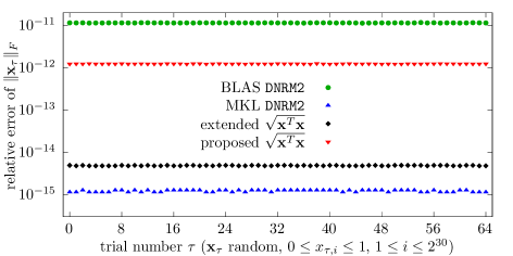
Figure 8: Relative errors of $\|\mathbf{x}_{\tau}\|_{F}$ computed by several procedures, for $\xi=0$.

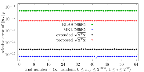
Figure 9: Relative errors of $\|\mathbf{x}_{\tau}\|_{F}$ computed by several procedures, for $\xi=1008$.

Figures 8 and 9 suggest that the reference BLAS routine is consistently about four orders of magnitude less accurate than the MKL’s $\mathtt{DNRM2}$. Also, the MKL’s routine is significantly more accurate than computing in extended precision, what indicates that the MKL does not use the reference algorithm in its published form.

Therefore, the MKL’s routine is the most accurate one, but bound to overflow at least when the actual result is not finitely representable in double precision, while Algorithm 17 (or the “proposed $\sqrt{\mathbf{x}^{T}\mathbf{x}}$”) and the computation of $\sqrt{\mathbf{x}^{T}\mathbf{x}}$ in extended precision cannot overflow for any reasonably-sized $\mathbf{x}$. However, from Figs. 10 and 11 it can be concluded that Algorithm 17 is somewhat slower that the extended dot-product, which in turn is significantly slower than the MKL’s $\mathtt{DNRM2}$. On the MKL-targeted platforms, its $\mathtt{DNRM2}$ is thus the method of choice for the Jacobi-type SVD, even if that entails a sporadic downscaling of the input data.

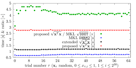
Figure 10: Performance of computing $\|\mathbf{x}_{\tau}\|_{F}$ by several procedures, for $\xi=0$.

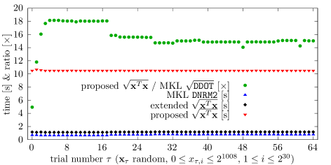
Figure 11: Performance of computing $\|\mathbf{x}_{\tau}\|_{F}$ by several procedures, for $\xi=1008$.

Vectorized quadruple precision

An accurate alternative way of computing $\sqrt{\mathbf{x}^{T}\mathbf{x}}$ without overflow is to use the SLEEF’s vectorized quad-precision math library by modifying Algorithm 15 to convert the loaded double precision vectors to quadruple precision ones and then call the vectorized quad-fma on them. Such an approach gives the results virtually indistinguishable from a non-vectorized quadruple dot-product, but in the testing environment, for $\xi=0$, it is $\approx 164\times$ and $\approx 1.69\times$ slower than the MKL’s $\mathtt{DDOT}$ and the BLAS $\mathtt{DNRM2}$, respectively, maybe because SLEEF does not yet provide the inlineable versions of its functions for the Intel’s compilers.

F.5 Conclusion

When the MKL’s $\mathtt{DNRM2}$ and the hardware-supported extended precision are not available, and the SLEEF’s vectorized quad-precision library happens to be too slow (or unavailable), the proposed $\sqrt{\mathbf{x}^{T}\mathbf{x}}$ method can be employed as a fail-safe option, either for computing $\|\mathbf{x}\|_{F}$ on its own, or to be called on the second attempt, after a faster but at least comparably accurate method overflows.

It is also easy to convert in a portable way the result of other methods in double, extended, or quadruple precision to the $(e,f)$ representation, which thus can be used for encoding the Frobenius norms of the columns of the iteration matrix in the Jacobi SVD, regardless of the chosen method of computing them. The remaining parts of the SVD algorithm do not rely on a higher precision of computation or of data, so a possible loss of it due to the rounding of $f$ to double precision is acceptable.

As $m$ becomes larger, and/or with an unfavorable distribution of the elements’ magnitudes, such that the huge elements precede the small ones, at a certain point the partial sums in the proposed algorithm can become too large to be (significantly) affected by the subsequent updates, resulting in a too small final norm and hence a big relative error. It is worth exploring if, e.g., three vector accumulators instead of one—for the small, the medium, and the large magnitudes, in the spirit of the Blue’s algorithm [8]—could improve the relative accuracy. However, such an approach will inevitably reduce the amount of the vector parallelism, since the present instructions have to be trebled and masked to affect the appropriate accumulator only.

Appendix G Addenda for Section 5

Section 5 from the main paper is here expanded.

G.1 Addendum for Section 5.2

For the eigenvector matrix $\Phi$ of a Hermitian matrix of order two holds $|\det\Phi|=c^{2}+|s|^{2}=1$, where $c=\cos\varphi$ and $s=\mathrm{e}^{\mathrm{i}\alpha}\sin\varphi$. Therefore, $\delta_{\Phi}^{\text{{x}}}=||\det(\mathop{\mathrm{fl}}(\Phi))|-1|$ determines how much the real cosine and the real or complex sine, computed by a routine designated by x, depart from the ones that would make $\Phi$ unitary. For a batch $\tau$, let $\delta_{\tau}^{\text{{x}}}=\max_{i}\delta_{\Phi_{\tau,i}}^{\text{{x}}}$, $1\leq i\leq 2^{28}$. Then, Fig. 12 shows that, in the real case, the batched and the LAPACK-based EVDs do not differ much in this measure of accuracy, but in the complex case the LAPACK-based ones may be several orders of magnitude less accurate. Together with Figs. 13 and 14, described below, this further explains Fig. 2.

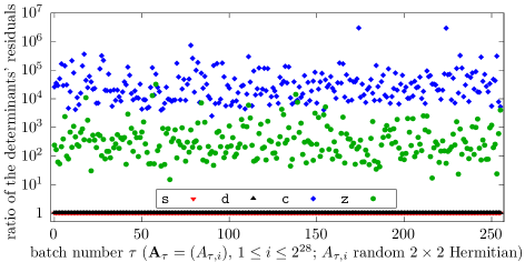
Figure 12: Per-batch ratios $\delta_{\tau}^{\text{{S}}}/\delta_{\tau}^{\text{{s}}}$, $\delta_{\tau}^{\text{{D}}}/\delta_{\tau}^{\text{{d}}}$, $\delta_{\tau}^{\text{{C}}}/\delta_{\tau}^{\text{{c}}}$, and $\delta_{\tau}^{\text{{Z}}}/\delta_{\tau}^{\text{{z}}}$ of the determinants’ residuals.

If a closer look is taken at the matrix $A_{\max}^{\delta}$ that caused the greatest determinant’s residual with CLAEV2, and at the computed outputs $\Lambda_{\max}^{\delta}$ and $U_{\max}^{\delta}$ (all in single precision, but printed out with $21$ digits after the decimal point for reproducibility),

$$A_{\max}^{\delta}=\begin{bmatrix}\text{{A}}&\text{{B}}\\ \bar{\text{{B}}}&\text{{C}}\end{bmatrix},\qquad\Lambda_{\max}^{\delta}=\begin{bmatrix}\text{{RT1}}&0\\ 0&\text{{RT2}}\end{bmatrix},\qquad U_{\max}^{\delta}=\begin{bmatrix}\text{{CS1}}&-\overline{\text{{SN1}}}\\ \text{{SN1}}&\hphantom{-}\text{{CS1}}\end{bmatrix},$$

where

$$\begin{gathered}\text{{A}}=-5.540058702080522136604\cdot 10^{-39},\\ \text{\framebox{$\text{{B}}=-1.401298464324817070924\cdot 10^{-45}+1.401298464324817070924\cdot 10^{-45}\mathrm{i}$}},\\ \text{{C}}=-5.832059874778063193026\cdot 10^{-39},\end{gathered}$$

and

$$\begin{gathered}\text{{RT1}}=\lambda_{1}=-5.832059874778063193026\cdot 10^{-39},\\ \text{{RT2}}=\lambda_{2}=-5.540058702080522136604\cdot 10^{-39};\\ \text{{CS1}}=\cos\varphi=-4.798947884410154074430\cdot 10^{-6},\\ \text{\framebox{\framebox{$\text{{SN1}}=\mathrm{e}^{\mathrm{i}\alpha}\sin\varphi=-1-\mathrm{i}$}}},\end{gathered}$$

a disastrous failure to represent $|\text{{B}}|$ in the subnormal range by any value other than $|\Re{\text{{B}}}|=|\Im{\text{{B}}}|$, as explained in Remark 2.4, becomes the obvious reason for the loss of accuracy. But why was $\sin\varphi$ computed as unity? The answer is that the eigenvalues had to be swapped to make $|\lambda_{1}|\geq|\lambda_{2}|$. Since CLAEV2 calls SLAEV2 with A, $|\text{{B}}|$, and C, the latter routine performed the exchange $\cos\varphi\leftarrow-\sin\varphi$, $\sin\varphi\leftarrow\cos\varphi$, as if the columns of its, real $U$ were swapped. Then CLAEV2 multiplied $\bar{\text{{B}}}/|\text{{B}}|=\mathrm{e}^{\mathrm{i}\alpha}=-1-\mathrm{i}$ by the new value of $\sin\varphi$, i.e., by unity. Note that if A and C changed roles, $\mathrm{e}^{\mathrm{i}\alpha}$ would have remained $-1-\mathrm{i}$, but it would have been multiplied by $\sin\varphi\approx 4.798947884\cdot 10^{-6}$. Even tough $\text{{CS1}}=-1$ then, $||\det{U}|-1|$ would have been small. Algorithm 2 ensures $|\sin\varphi|\leq 1/\sqrt{2}$, up to the rounding errors, so a bogus $\mathrm{e}^{\mathrm{i}\alpha}$ is always scaled down.

As already known for the LAPACK’s EVD, the smaller eigenvalue by magnitude might not be computed with any relative accuracy, and this is also the case with the batched EVD. The normwise residuals $\lambda_{F}^{\text{{x}},\tau}=\max_{i}\|\mathop{\mathrm{fl}}(\Lambda_{\tau,i})-\Lambda_{\tau,i}\|_{F}/\|\Lambda_{\tau,i}\|_{F}$, however, seem stable, and their ratios are shown in Fig. 13. The values below unity indicate when the batched EVD was less accurate, while those above unity demonstrate that in a majority of batches the LAPACK-based EVD was more inaccurate.

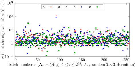
Figure 13: Per-batch ratios $\lambda_{F}^{\text{{S}},\tau}/\lambda_{F}^{\text{{s}},\tau}$, $\lambda_{F}^{\text{{D}},\tau}/\lambda_{F}^{\text{{d}},\tau}$, $\lambda_{F}^{\text{{C}},\tau}/\lambda_{F}^{\text{{c}},\tau}$, and $\lambda_{F}^{\text{{Z}},\tau}/\lambda_{F}^{\text{{z}},\tau}$ of the eigenvalues’ normwise residuals.

A similar conclusion holds for the eigenvalue larger by magnitude, $\lambda_{\max}$, that is always computed relatively accurate, up to a modest constant times $\varepsilon$. Figure 14 shows the ratios of the $\max$-residuals, $\lambda_{\max}^{\text{{x}},\tau}=\max_{i}|\mathop{\mathrm{fl}}(\lambda_{\max;\tau,i})-\lambda_{\max;\tau,i}|/|\lambda_{\max;\tau,i}|$.

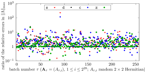
Figure 14: Per-batch ratios $\lambda_{\max}^{\text{{S}},\tau}/\lambda_{\max}^{\text{{s}},\tau}$, $\lambda_{\max}^{\text{{D}},\tau}/\lambda_{\max}^{\text{{d}},\tau}$, $\lambda_{\max}^{\text{{C}},\tau}/\lambda_{\max}^{\text{{c}},\tau}$, and $\lambda_{\max}^{\text{{Z}},\tau}/\lambda_{\max}^{\text{{z}},\tau}$ of the eigenvalues’ $\max$-residuals.

G.2 Addendum for Section 5.3

Figures 15 and 16 show the number of sweeps until convergence in the real and the complex case on $\Xi_{1}^{\mathbb{F}}$ and $\Xi_{2}^{\mathbb{F}}$, respectively, while Figs. 17, 18 and 19 correspond to Figs. 3, 4 and 5, respectively, in the real case on $\Xi_{1}^{\mathbb{R}}$.

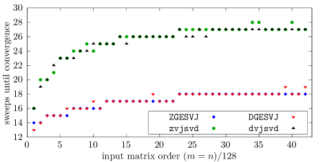
Figure 15: Number of sweeps until convergence for the LAPACK’s xGESVJ and the proposed routines (with the $\mathtt{MM}$ parallel quasi-cyclic pivot strategy), on $\Xi_{1}^{\mathbb{F}}$.

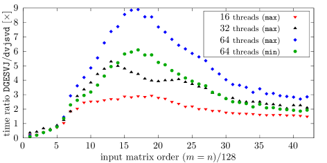
Figure 17: Run-time ratios of DGESVJ and $\mathtt{dvjsvd}$ with $\mathtt{MM}$ on $\Xi_{1}^{\mathbb{R}}$.

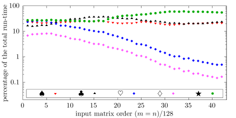
Figure 18: Breakdown of the run-time of $\mathtt{dvjsvd}$ with $\mathtt{MM}$ on $\Xi_{1}^{\mathbb{R}}$ with $64$ threads.

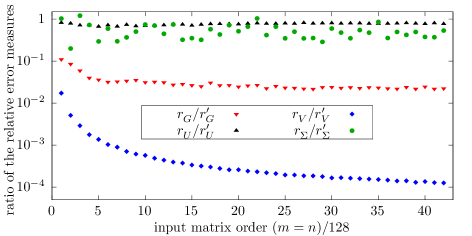
Figure 19: Ratios of the relative error measures for the SVDs on $\Xi_{1}^{\mathbb{R}}$.

G.2.1 Performance of several double precision routines

Performance of several sequential double precision MKL routines (DDOT, DROT) and the similar ones proposed here ($\mathtt{ddpscl}^{\prime}$, $\mathtt{djrotf}$) were compared in terms of giga ($10^{9}$) floating-point operations per second, i.e., GFLOP/s. The routines’ FLOP counts are taken as

(71) $$\mathop{\mathrm{FLOP}}(n)=\begin{cases}n,&\text{{DDOT} ($1$ {fma} per row of both arrays)},\\ 4n,&\text{{DROT} ($1$ {fma}, $1$ {mul} per row of each array)},\\ 18n+35,&\text{$\mathtt{ddpscl}^{\prime}$ (\text{see \lx@cref{creftype~refnum}{a:ddpsclcs}})},\\ 4n,&\text{$\mathtt{djrotf}$ ($1$ {fma}, $1$ {mul} per row of each array)},\end{cases}$$

where $n$ is the length of two input arrays of each routine, $\mathtt{djrotf}$ is the “fast” variant of $\mathtt{djrot}$ without the norm approximation, fma is the fused multiply-add operation, scalef is the scaling by a power of two, and mul is the floating-point multiplication.

Figure 20 shows the testing results for $n=128i$, $1\leq i\leq 42$. Reliability of timing was ensured by calling each routine with different random inputs $100000$ times. Observe that $\mathtt{ddpscl}^{\prime}$ is more performant than DDOT since the former does more arithmetical processing with each input loaded from the memory (by scaling the arrays’ elements in both its implementations, and by using the compensated summation in the enhanced one, which was timed), while $\mathtt{djrotf}$ and DROT are similar performance-wise.

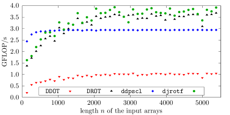
Figure 20: Performance in GFLOP/s for various double precision routines.

It is harder to figure out the exact implementation of complex arithmetic in the MKL routines and deduce the FLOP counts from that. The complex routines’ execution could be profiled and the retired floating-point instructions counted, what would be an effort worth taking if the similar complex routines proposed here were known to be optimized to the fullest extent possible. This is therefore left for future work.

Appendix H The single precision variants of the parallel Jacobi SVD method

The single precision implementation is conceptually identical to the double precision one, with the necessary changes for the datatype and the associated range of values. For brevity, the pseudocode of the single precision routines is omitted and the readers are referred to the actual source code on GitHub, while bearing in mind that $\mathtt{s}=16$.

Two single precision datasets, $\Xi_{3}^{\mathbb{R}}$ and $\Xi_{3}^{\mathbb{C}}$, were generated similarly to $\Xi_{1}^{\mathbb{R}}$ and $\Xi_{1}^{\mathbb{C}}$, respectively (see Section 5.1), but with $\xi_{3}=-12$. Figure 21 corresponds to Fig. 15, showing that significantly more sweeps were also required for convergence under parallel than under serial pivot strategies in the single precision case. Figures 22 and 24, compared to Figs. 3 and 17, respectively, show similar speedup profiles, albeit with a bit higher peaks and the larger matrix orders for which they were attained. Figures 23 and 25 depict the percentages of run-time of the key routines comparable to those on Figures 4 and 18. Figures 26 and 27 show similar relative error ratios as Figs. 5 and 19, respectively.

For the $\mathtt{sdpscl}$ routine in Fig. 28 the FLOP count was taken as $18n+67$, while the counts for the other routines remained the same as in Eq. 71. Compared to Fig. 20, SROT and $\mathtt{sdpscl}$ were noticeably less performant than their double precision counterparts, what remains to be explained. Apart from that, the testing results of the single precision real and complex variants of the SVD method are generally consistent with those of the double precision real and complex ones, respectively.

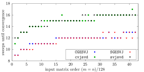
Figure 21: Number of sweeps until convergence for the LAPACK’s xGESVJ and the proposed routines (with the $\mathtt{MM}$ parallel quasi-cyclic pivot strategy), on $\Xi_{3}^{\mathbb{F}}$.

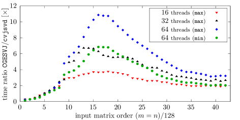
Figure 22: Run-time ratios of CGESVJ and $\mathtt{cvjsvd}$ with $\mathtt{MM}$ on $\Xi_{3}^{\mathbb{C}}$.

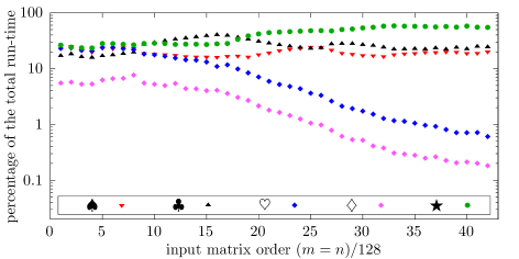
Figure 23: Breakdown of the run-time of $\mathtt{cvjsvd}$ with $\mathtt{MM}$ on $\Xi_{3}^{\mathbb{C}}$ with $64$ threads.

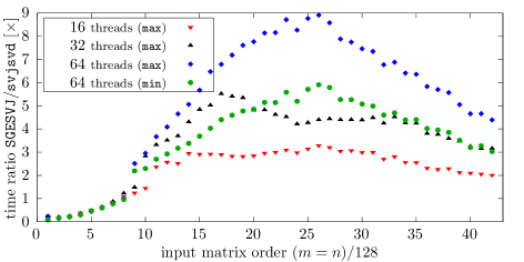
Figure 24: Run-time ratios of SGESVJ and $\mathtt{svjsvd}$ with $\mathtt{MM}$ on $\Xi_{3}^{\mathbb{R}}$.

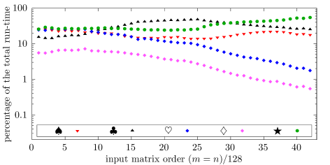
Figure 25: Breakdown of the run-time of $\mathtt{svjsvd}$ with $\mathtt{MM}$ on $\Xi_{3}^{\mathbb{R}}$ with $64$ threads.

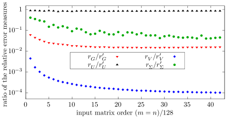
Figure 26: Ratios of the relative error measures for the SVDs on $\Xi_{3}^{\mathbb{C}}$.

Figure 27: Ratios of the relative error measures for the SVDs on $\Xi_{3}^{\mathbb{R}}$.

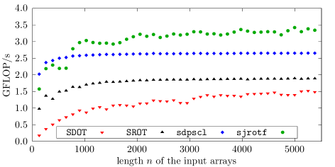
Figure 28: Performance in GFLOP/s for various single precision routines.

Appendix I Vectorization of the Gram–Schmidt orthogonalization

The complex Gram–Schmidt orthogonalization is vectorized in Algorithm 18, and the real one in Algorithm 19, both shown in double precision. The actual implementation of these algorithms also includes the $\max$-norm estimation of $\mathop{\mathrm{fl}}(g_{q}^{\prime})$, in the same vein as in Algorithm 7, but it has been omitted from their presentation here for brevity.

Algorithm 18 $\mathtt{zgsscl}$: a vectorized complex Gram–Schmidt orthogonalization.

0:  $a_{21}^{\prime}=(\Re{a_{21}^{\prime}},\Im{a_{21}^{\prime}});\quad g_{p}=(\Re{g_{p}},\Im{g_{p}}),\ g_{q}=(\Re{g_{q}},\Im{g_{q}});$$0<\|g_{p}\|_{F}=(e_{p},f_{p}),\ 0<\|g_{q}\|_{F}=(e_{q},f_{q});$

0:  $\mathop{\mathrm{fl}}(g_{q}^{\prime})$ from Eq. 29.

1:  $\mathsf{e}_{q}=\mathop{\mathtt{set1}}(e_{q});\quad-\mathsf{e}_{p}=\mathop{\mathtt{set1}}(-e_{p});\quad-\mathsf{e}_{q}=\mathop{\mathtt{set1}}(-e_{q});\quad f_{q/p}=f_{q}/f_{p};$

2:  $-\Re{\bm{\psi}}=\mathop{\mathtt{set1}}(-\Re{a_{21}^{\prime}}\cdot f_{q/p});\quad-\Im{\bm{\psi}}=\mathop{\mathtt{set1}}(\Im{a_{21}^{\prime}\cdot f_{q/p}});$ /​/ $-\bm{\psi}=-a_{21}^{\prime\ast}\cdot f_{q/p};$

3:  for $\mathtt{i}=0$ to $\tilde{m}-1$ step $\mathtt{s}$ do /​/ sequentially

4:     $\Re{\mathsf{x}}=\mathop{\mathtt{load}}(\Re{g_{p}}+\mathtt{i});\quad\Im{\mathsf{x}}=\mathop{\mathtt{load}}(\Im{g_{p}}+\mathtt{i});$ /​/ load a chunk of $g_{p}$

5:     $\Re{\mathsf{x}^{\prime}}=\mathop{\mathtt{scalef}}(\Re{\mathsf{x}},-\mathsf{e}_{p});\quad\Im{\mathsf{x}^{\prime}}=\mathop{\mathtt{scalef}}(\Im{\mathsf{x}},-\mathsf{e}_{p});$ /​/ $\mathsf{x}^{\prime}=\mathsf{2}^{-\mathsf{e}_{p}}\mathsf{x}$

6:     $\Re{\mathsf{y}}=\mathop{\mathtt{load}}(\Re{g_{q}}+\mathtt{i});\quad\Im{\mathsf{y}}=\mathop{\mathtt{load}}(\Im{g_{q}}+\mathtt{i});$ /​/ load a chunk of $g_{q}$

7:     $\Re{\mathsf{y}^{\prime}}=\mathop{\mathtt{scalef}}(\Re{\mathsf{y}},-\mathsf{e}_{q});\quad\Im{\mathsf{y}^{\prime}}=\mathop{\mathtt{scalef}}(\Im{\mathsf{y}},-\mathsf{e}_{q});$ /​/ $\mathsf{y}^{\prime}=\mathsf{2}^{-\mathsf{e}_{q}}\mathsf{y}$

8:     $\Re{\mathsf{y}^{\prime}}=\mathop{\mathtt{scalef}}(\mathop{\mathtt{fmadd}}(-\Re{\bm{\psi}},\Re{\mathsf{x}^{\prime}},\mathop{\mathtt{fnmadd}}(-\Im{\bm{\psi}},\Im{\mathsf{x}^{\prime}},\Re{\mathsf{y}^{\prime}})),\mathsf{e}_{q});$ /​/ $\Re{\lx@cref{creftype~refnum}{e:GS}}$

9:     $\Im{\mathsf{y}^{\prime}}=\mathop{\mathtt{scalef}}(\mathop{\mathtt{fmadd}}(-\Re{\bm{\psi}},\Im{\mathsf{x}^{\prime}},\mathop{\mathtt{fmadd}}(-\Im{\bm{\psi}},\Re{\mathsf{x}^{\prime}},\Im{\mathsf{y}^{\prime}})),\mathsf{e}_{q});$ /​/ $\Im{\lx@cref{creftype~refnum}{e:GS}}$

10:     $\mathop{\mathtt{store}}(\Re{g_{q}}+\mathtt{i},\Re{\mathsf{y}^{\prime}});\quad\mathop{\mathtt{store}}(\Im{g_{q}}+\mathtt{i},\Im{\mathsf{y}^{\prime}});$ /​/ store $g_{q}^{\prime}$

11:  end for/​/ $g_{q}\to g_{q}^{\prime}$, $g_{p}$ unchanged

Algorithm 19 $\mathtt{dgsscl}$: a vectorized real Gram–Schmidt orthogonalization.

0:  $a_{21}^{\prime};\quad g_{p},\ g_{q};\quad 0<\|g_{q}\|_{F}=(e_{q},f_{q}),\ 0<\|g_{p}\|_{F}=(e_{p},f_{p});$.

0:  $\mathop{\mathrm{fl}}(g_{q}^{\prime})$ from Eq. 29.

1:  $\mathsf{e}_{q}=\mathop{\mathtt{set1}}(e_{q});\ -\mathsf{e}_{p}=\mathop{\mathtt{set1}}(-e_{p});\ -\mathsf{e}_{q}=\mathop{\mathtt{set1}}(-e_{q});\ -\bm{\psi}=\mathop{\mathtt{set1}}(-a_{21}^{\prime}(f_{q}/f_{p}));$

2:  for $\mathtt{i}=0$ to $\tilde{m}-1$ step $\mathtt{s}$ do /​/ sequentially

3:     $\mathsf{x}=\mathop{\mathtt{load}}(g_{p}+\mathtt{i});\qquad\mathsf{y}=\mathop{\mathtt{load}}(g_{q}+\mathtt{i});$ /​/ scaling by a power of two is …

4:     $\mathsf{x}=\mathop{\mathtt{scalef}}(\mathsf{x},-\mathsf{e}_{p});\qquad\mathsf{y}=\mathop{\mathtt{scalef}}(\mathsf{y},-\mathsf{e}_{q});$ /​/ … faster than full division

5:     $\mathsf{y}=\mathop{\mathtt{scalef}}(\mathop{\mathtt{fmadd}}(-\bm{\psi},\mathsf{x},\mathsf{y}),\mathsf{e}_{q});\qquad\mathop{\mathtt{store}}(g_{q}+\mathtt{i},\mathsf{y});$ /​/ Eq. 29

6:  end for/​/ $g_{q}\to g_{q}^{\prime}$, $g_{p}$ unchanged

A test $16\times 16$ matrix for the method with Algorithm 19 was constructed as:

$$G_{ij}=\begin{cases}2^{\hat{\eta}-(j-1)-|i-j|},&1\leq j\leq 8,\\ 2^{-51-(j-1)-|i-j|},&9\leq j\leq 16,\end{cases}$$

bearing in mind that $\upsilon=2^{-53}\sqrt{16}=2^{-51}$ (see Section 3.5.1). Of 128 transformations in the first three $\mathtt{MM}$ sweeps, 72 were the Gram–Schmidt orthogonalization, as well as 48 of 68 transformations in the last non-empty sweep, with $r_{G}^{\prime}\approx 1.095015\cdot 10^{-15}$, compared to $r_{G}\approx 3.220344\cdot 10^{-16}$ from DGESVJ on $G$ with an extra sweep.

Appendix J The batched eigendecomposition of Hermitian matrices of order two in CUDA

The serial code from Listing LABEL:l:1 can easily be converted into a CUDA kernel. In the lines 9 and 10 the CUDA integer device function $\mathtt{min}$ can be used instead of the ternary operators, and the double precision intrinsics elsewhere instead of the basic arithmetic operators and functions, e.g., $\mathtt{\_\_fma\_rn}$ instead of $\mathtt{fma}$, $\mathtt{\_\_dsqrt\_rn}$ instead of $\mathtt{sqrt}$, and $\mathop{\mathtt{\_\_drcp\_rn}}(x)$ instead of computing $1/x$.

The layout of the input and the output data is the same as in the vectorized algorithm from Section 2.4, apart from the permutation bit $p$ and $\zeta$, which are returned packed in an integer. A GPU thread reads the elements of its matrix $A$ and stores the results at the offset (size_t)(blockIdx.x) * blockDim.x + threadIdx.x, where each thread block in a onedimensional execution grid has $64$ threads (two warps).

Since each thread processes its own matrix independently of the other threads, there are neither intra-block nor inter-block data dependencies. A kernel can also be converted into a device function, to be incorporated into larger kernels, and the data can be read from and/or be written to the shared instead of the global memory.

Figure 29 shows the timing results (without the data transfers) of the real and the complex kernels in single and double precision on an NVIDIA GeForce GTX TITAN X (a Maxwell series GPU, sm_52 architecture), with the CUDA Toolkit version 11.7.0. The input batches consisted of $2^{27}$ Hermitian matrices of order two each. It is expected that on newer GPU architectures the run times should be substantially lower.

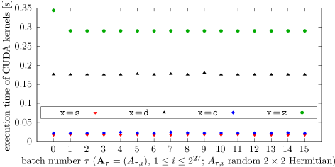
Figure 29: Run-times of the CUDA batched Hermitian $2\times 2$ EVD kernels.

References

- [1] A. Abdelfattah, H. Anzt, J. Dongarra, M. Gates, A. Haidar, J. Kurzak, P. Luszczek, S. Tomov, I. Yamazaki, and A. YarKhan, Linear algebra software for large-scale accelerated multicore computing, Acta Numer., 25 (2016), pp. 1–160, https://doi.org/10.1017/S0962492916000015.
- [2] A. Abdelfattah, T. Costa, J. Dongarra, M. Gates, A. Haidar, S. Hammarling, N. J. Higham, J. Kurzak, P. Luszczek, S. Tomov, and M. Zounon, A set of batched basic linear algebra subprograms and LAPACK routines, ACM Trans. Math. Software, 47 (2021), pp. 1–23 (art. no. 21), https://doi.org/10.1145/3431921.
- [3] E. Anderson, Algorithm 978: Safe scaling in the Level 1 BLAS, ACM Trans. Math. Software, 44 (2017), pp. 1–28 (art. no. 12), https://doi.org/10.1145/3061665.
- [4] E. Anderson, Z. Bai, C. Bischof, S. Blackford, J. Demmel, J. Dongarra, J. Du Croz, A. Greenbaum, S. Hammarling, A. McKenney, and D. Sorensen, LAPACK Users’ Guide, Software, Environments and Tools, SIAM, Philadelphia, PA, USA, ed., 1999, https://doi.org/10.1137/1.9780898719604.
- [5] K. E. Batcher, Sorting networks and their applications, in Proceedings of the April 30–May 2, 1968, Spring Joint Computer Conference, vol. 32 of AFIPS ’68 (Spring), New York, NY, USA, 1968, Association for Computing Machinery, pp. 307–314, https://doi.org/10.1145/1468075.1468121.
- [6] M. Bečka, G. Okša, and M. Vajteršic, Dynamic ordering for a parallel block-Jacobi SVD algorithm, Parallel Comp., 28 (2002), pp. 243–262, https://doi.org/10.1016/S0167-8191(01)00138-7.
- [7] M. Bečka, G. Okša, and M. Vajteršic, New dynamic orderings for the parallel one-sided block-Jacobi SVD algorithm, Parallel Process. Lett., 25 (2015), pp. 1–19 (art. no. 1550003), https://doi.org/10.1142/S0129626415500036.
- [8] J. L. Blue, A portable Fortran program to find the Euclidean norm of a vector, ACM Trans. Math. Software, 4 (1978), pp. 15–23, https://doi.org/10.1145/355769.355771.
- [9] W. H. Boukaram, G. Turkiyyah, H. Ltaief, and D. E. Keyes, Batched QR and SVD algorithms on GPUs with applications in hierarchical matrix compression, Parallel Comp., 74 (2018), pp. 19–33, https://doi.org/10.1016/j.parco.2017.09.001.
- [10] B. Bramas, A novel hybrid quicksort algorithm vectorized using AVX-512 on Intel Skylake, Int. J. Adv. Comput. Sci. Appl., 8 (2017), pp. 337–344, https://doi.org/10.14569/IJACSA.2017.081044.
- [11] P. P. M. de Rijk, A one-sided Jacobi algorithm for computing the singular value decomposition on a vector computer, SIAM J. Sci. and Stat. Comput., 10 (1989), pp. 359–371, https://doi.org/10.1137/0910023.
- [12] J. Demmel and K. Veselić, Jacobi’s method is more accurate than QR, SIAM J. Matrix Anal. Appl., 13 (1992), pp. 1204–1245, https://doi.org/10.1137/0613074.
- [13] I. S. Dhillon and B. N. Parlett, Orthogonal eigenvectors and relative gaps, SIAM J. Matrix Anal. Appl., 25 (2003), pp. 858–899, https://doi.org/10.1137/S0895479800370111.
- [14] I. S. Dhillon and B. N. Parlett, Multiple representations to compute orthogonal eigenvectors of symmetric tridiagonal matrices, Linear Algebra Appl., 387 (2004), pp. 1–28, https://doi.org/10.1016/j.laa.2003.12.028.
- [15] T. Dong, A. Haidar, S. Tomov, and J. Dongarra, Accelerating the SVD bi-diagonalization of a batch of small matrices using GPUs, J. Comput. Sci., 26 (2018), pp. 237–245, https://doi.org/10.1016/j.jocs.2018.01.007.
- [16] Z. Drmač, Implementation of Jacobi rotations for accurate singular value computation in floating point arithmetic, SIAM J. Sci. Comput., 18 (1997), pp. 1200–1222, https://doi.org/10.1137/S1064827594265095.
- [17] Z. Drmač and K. Veselić, New fast and accurate Jacobi SVD algorithm. I, SIAM J. Matrix Anal. Appl., 29 (2008), pp. 1322–1342, https://doi.org/10.1137/050639193.
- [18] Z. Drmač and K. Veselić, New fast and accurate Jacobi SVD algorithm. II, SIAM J. Matrix Anal. Appl., 29 (2008), pp. 1343–1362, https://doi.org/10.1137/05063920X.
- [19] J. G. F. Francis, The QR transformation—part 1, Comput. J., 4 (1961), pp. 265–271, https://doi.org/10.1093/comjnl/4.3.265.
- [20] J. G. F. Francis, The QR transformation—part 2, Comput. J., 4 (1962), pp. 332–345, https://doi.org/10.1093/comjnl/4.4.332.
- [21] S. Graillat, C. Lauter, P. T. P. Tang, N. Yamanaka, and S. Oishi, Efficient calculations of faithfully rounded -norms of -vectors, ACM Trans. Math. Software, 41 (2015), pp. 1–20 (art. no. 24), https://doi.org/10.1145/2699469.
- [22] V. Hari and E. Begović Kovač, On the convergence of complex Jacobi methods, Linear Multilinear Algebra, 69 (2021), pp. 489–514, https://doi.org/10.1080/03081087.2019.1604622.
- [23] IEEE Computer Society, 754-2019 - IEEE Standard for Floating-Point Arithmetic, IEEE, New York, NY, USA, July 2019, https://doi.org/10.1109/IEEESTD.2019.8766229.
- [24] Intel Corp., Intel® 64 and IA-32 Architectures Software Developer’s Manual, June 2021. https://software.intel.com/en-us/articles/intel-sdm (Order No. 325462-075US, Combined Volumes: 1, 2A, 2B, 2C, 2D, 3A, 3B, 3C, 3D and 4).
- [25] ISO/IEC JTC1/SC22/WG14, ISO/IEC 9899:2018(en) Information technology — Programming languages — C, ISO, ed., 2018. International standard.
- [26] C. G. J. Jacobi, Über ein leichtes Verfahren die in der Theorie der Säcularstörungen vorkommenden Gleichungen numerisch aufzulösen, J. Reine Angew. Math., 30 (1846), pp. 51–94, https://doi.org/10.1515/crll.1846.30.51.
- [27] C.-P. Jeannerod and S. M. Rump, Improved error bounds for inner products in floating-point arithmetic, SIAM J. Matrix Anal. Appl., 34 (2013), pp. 338–344, https://doi.org/10.1137/120894488.
- [28] W. Kahan, Further remarks on reducing truncation errors, Comm. ACM, 8 (1965), p. 40, https://doi.org/10.1137/0914050.
- [29] E. G. Kogbetliantz, Solution of linear equations by diagonalization of coefficients matrix, Quart. Appl. Math., 13 (1955), pp. 123–132, https://doi.org/10.1090/qam/88795.
- [30] M. Mantharam and P. J. Eberlein, Block recursive algorithm to generate Jacobi–sets, Parallel Comput., 19 (1993), pp. 481–496, https://doi.org/10.1016/0167-8191(93)90001-2.
- [31] W. F. Mascarenhas, On the convergence of the Jacobi method for arbitrary orderings, SIAM J. Matrix Anal. Appl., 16 (1995), pp. 1197–1209, https://doi.org/10.1137/S0895479890179631.
- [32] O. Møller, Quasi double-precision in floating point addition, BIT, 5 (1965), pp. 37–50, https://doi.org/10.1007/BF01975722.
- [33] J.-M. Muller, N. Brisebarre, F. de Dinechin, C.-P. Jeannerod, V. Lefèvre, G. Melquiond, N. Revol, D. Stehlé, and S. Torres, Handbook of Floating-Point Arithmetic, Birkhäuser, Boston, 2010, https://doi.org/10.1007/978-0-8176-4705-6.
- [34] V. Novaković, A hierarchically blocked Jacobi SVD algorithm for single and multiple graphics processing units, SIAM J. Sci. Comput., 37 (2015), pp. C1–C30, https://doi.org/10.1137/140952429.
- [35] V. Novaković, Batched computation of the singular value decompositions of order two by the AVX-512 vectorization, Parallel Process. Lett., 30 (2020), pp. 1–23 (art. no. 2050015), https://doi.org/10.1142/S0129626420500152.
- [36] V. Novaković and S. Singer, A GPU-based hyperbolic SVD algorithm, BIT, 51 (2011), pp. 1009–1030, https://doi.org/10.1007/s10543-011-0333-5.
- [37] V. Novaković and S. Singer, Implicit Hari–Zimmermann algorithm for the generalized SVD on the GPUs, Int. J. High Perform. Comput. Appl., 35 (2021), pp. 170–205, https://doi.org/10.1177/1094342020972772.
- [38] V. Novaković and S. Singer, A Kogbetliantz-type algorithm for the hyperbolic SVD, Numer. Algorithms, 90 (2022), pp. 523–561, https://doi.org/10.1007/s11075-021-01197-4.
- [39] N. Shibata and F. Petrogalli, SLEEF: A portable vectorized library of C standard mathematical functions, IEEE Trans. Parallel Distrib. Syst., 31 (2020), pp. 1316–1327, https://doi.org/10.1109/TPDS.2019.2960333.
- [40] S. Singer, E. Di Napoli, V. Novaković, and G. Čaklović, The LAPW method with eigendecomposition based on the Hari–Zimmermann generalized hyperbolic SVD, SIAM J. Sci. Comput., 42 (2020), pp. C265–C293, https://doi.org/10.1137/19M1277813.
- [41] F. G. V. Zee and T. M. Smith, Implementing high-performance complex matrix multiplication via the 3m and 4m methods, ACM Trans. Math. Software, 44 (2017), pp. 1–36 (art. no. 7), https://doi.org/10.1145/3086466.